1. No category

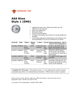
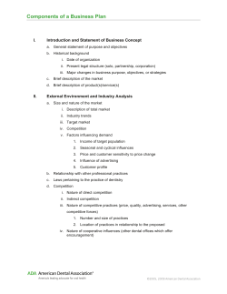
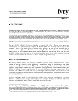
Chapter 1
The DASCh Experience:
How to Model a Supply Chain
H. Van Dyke Parunak
Center for Electronic Commerce, ERIM
3600 Green Court, Suite 550
Ann Arbor, MI 48105
[email protected]
1.1. Introduction
Nonlinear dynamical systems have been a fertile field for the application of
simulation techniques. Since the 1960’s, System Dynamics has studied such problems
by integrating systems of ordinary differential equations (ODE’s) over time. More
recently, increases in computer power have permitted the broad application of agentbased (or individual-based) modeling. In our work on supply chain modeling, we
have found agent-based modeling to be more flexible than ODE models for basic
exploration. One phenomenon we discovered, the inventory oscillator, can also be
modeled in ODE’s, an approach that permits more rapid manipulation in a
spreadsheet environment. Further study permits derivation of a closed-form analytical
model as well, which makes explicit a number of interesting structural features of the
oscillator.
This paper does not pretend to enrich the repertoire of nontrivial behaviors known
to complexity researchers. Mathematically, the behavior we observe is not
particularly sophisticated: the inventory oscillator turns out to be computing a
modulus function. Its intended contribution is twofold. First, and primarily, we seek
to highlight the differences among agent-based, equation-based, and analytical system
modeling, in terms of when they can be applied and the results one can expect to
derive. The comparative simplicity of our system is what makes the analytical
treatment possible at all. Second, manufacturing engineers find the potential for
inventory fluctuation under stable boundary conditions counterintuitive and of great
practical import. Its reducibility to the modulus function, far from making the results
trivial, suggests that similar threshold nonlinearities may be responsible for other
unexpected time-varying manufacturing measurements, and thus points the way to
stabilize these important commercial systems.
Section 2 of this paper describes the supply chain problem. Section 3 reports the
three models that we constructed. Section 4 reviews the roles of each model and
recommendations for their deployment. Section 5 summarizes our conclusions.
2
The DASCh Experience
(
OEMs
"
'
First Tier
Supplier
#
&
&
"
'
"
&
)
#
$
%
&
'
Sub-Tier
Suppliers
!
*
+
,
-
/
.
Figure 1. A Simple Automotive Supply Network
1.2. The Supply Chain Challenge
Modern industrial strategists are developing the vision of the “virtual enterprise,”
formed for a particular market opportunity from independent firms with well-defined
core competencies [4]. The manufacturer of a complex product (the original
equipment manufacturer, or “OEM”) may purchase half or even more of the content
in the product from other firms. For example, an automotive manufacturer might buy
seats from one company, brake systems from another, air conditioning from a third,
and electrical systems from a fourth, and manufacture only the chassis, body, and
powertrain in its own facilities. The suppliers of major subsystems (such as seats) in
turn purchase much of their content from still other companies. As a result, the
“production line” that turns raw materials into a vehicle is a “supply network” (more
commonly though less precisely called a “supply chain”) of many different firms.
Figure 1 illustrates part of a simple supply network [1, 3]. Johnson Controls
supplies seating systems to Ford, General Motors, and Chrysler, and purchases
components and subassemblies either directly or indirectly from over 150 other
companies, some of which also supply one another. Product design and production
schedule must be managed across all these firms to produce quality vehicles on time
and at reasonable cost. Historically, this vision has been frustrated by unexpected
behavior of the supply network, such as large swings in orders and inventories and
unreliable information. Our research explores these problems from a dynamical
systems perspective.
1.3. Three Models
We have modeled one aspect of supply chain behavior using three different
approaches. Our initial agent-based model exhibited internal inventory oscillations
The DASCh Experience
3
under stable conditions at the chain’s boundaries. We replicated much of this
behavior in an equation-based model using ODE’s. Then we developed an analytical
model in which we could prove certain empirically observed characteristics of the
oscillator.
1.3.1. Agent-Based Model
The DASCh project (Dynamical Analysis of Supply Chains) [5, 6] includes three
species of agents. Company agents represent the different firms that trade with one
another in a supply network. They consume inputs from their suppliers and transform
them into outputs that they send to their customers. PPIC agents model the
Production Planning and Inventory Control algorithms used by company agents to
determine what inputs to order from their suppliers, based on the orders they have
received from their customers. These PPIC agents currently support a simple material
requirements planning (MRP) model.1 Shipping agents model the delay and
uncertainty involved in the movement of both material and information between
trading partners.
The initial DASCh experiments involve a supply chain with four company agents
(Figure 2: a boundary supplier, a boundary consumer, and two intermediate firms
producing a product with neither assembly nor disassembly). Each intermediate
company agent has a PPIC agent. Shipping agents move both material and
information among company agents.
We expected this simple structure to exhibit relatively uninteresting behavior, on
which the impact of successive modifications could be studied. In fact, it shows a
range of interesting behaviors in terms of the variability in orders and inventories of
the various company agents.
We
found
four
Site 1
different behaviors in the
(Consumer)
Pr
model: amplification of
od
Shipper 1
uc
variance in the order
tF
low
Mailer
1
stream as one moves
away from the customer,
Shipper 2
PPIC1 Site 2
induction of spurious
correlations in the order
stream, persistence of
Mailer 2
Shipper 3
disturbances long after a
Inf
Site 3
PPIC2
o
rm
single change in orders
ati
on
has been made, and
Site 4
Flo
generation of variation in
(Supplier)
w
Mailer 3
inventory levels in the
system
when
the
Figure 2. The DASCh Supply Chain.
boundary conditions are
1
The basic MRP algorithm includes developing a forecast of future demand based either on
past demand or on customer forecast (depending on location in the hourglass), estimating
inventory changes through time due to processing, deliveries, and shipments, determining
when inventory is in danger of falling below specified levels, and placing orders to replenish
inventory early enough to allow for estimated delivery times of suppliers.
4
The DASCh Experience
Inventory
Inventory
Inventory
held constant. Details of these
Site 2
120
behaviors are discussed in [6].
Site 3
100
This report focuses on the last
80
effect, the generation of inventory
60
variation. Even when top-level
40
demand is constant and bottom20
level supply is completely
0
reliable, intermediate sites can
0
50
100
150
generate complex oscillations in
Time
inventory levels, including phase
Figure 3. Demand/Capacity = 110/100
locking and multiperiodicity, as a
result of capacity limitations.
The consumer has a steady demand with no superimposed noise. The bottom-level
supplier makes every shipment exactly when promised, exactly in the amount
promised. Batch sizes are 1, but we impose a capacity limit on sites 2 and 3: at each
time step they can process only 100 parts, a threshhold nonlinearity. As long as the
consumer’s demand is below the capacity of the producers, the system quickly
stabilizes to constant ordering
levels and inventory throughout
160
the chain. When the consumer
140
demand exceeds the capacity of
120
100
the producers, inventory levels in
80
those sites begin to oscillate. The
60
basic dynamic is that filling
40
20
orders draws down inventory to
0
make up a shortfall in production.
120
170
220
When inventory falls too low, the
Site 2 Inventory
Time
Site 3 Inventory
current order is backlogged and
the current production run
Figure 4. Demand/Capacity = 150/100
provides a new inventory.
Figure 3 shows the behavior when demand exceeds capacity by 10%. Site
inventories oscillate out of phase with one another, in a sawtooth that rises rapidly
and then drops off gradually. The inventory variation ranges from near-zero to the
level of demand, much greater than the excess of demand over capacity
Figure 4 shows the dynamics after increasing consumer demand to 150. The
inventories follow a sawtooth of shorter period. Now one cycle’s production of 100
can support only two orders,
250
leading
to a
period-three
200
oscillation. The inventories of
150
sites 2 and 3, out of synch when
100
Demand/Capacity = 110/100,
50
become synchronized and in
phase after a transition period.
0
250
300
350
400
The transition period is
Time
actually longer than appears from
Figure 4. The increase from 110
Figure 5. Demand/Capacity = 220/100 (Site 2)
to 150 takes place at time 133, but
The DASCh Experience
5
the first evidence of it in site 2’s dynamics appears at time 145. The delay is due to
the backlog of over-capacity orders at the 110 level, which must be cleared before the
new larger orders can be processed.
Figure 5 shows the result of increasing the overload even further. (Because of the
increased detail in the dynamics, we show only the inventory level for site 2.) Now
the consumer is ordering 220 units per time period. Again, backlogged orders at the
previous level delay the appearance of the new dynamics: demand changes at time
228, but appears in the dynamics first at time 288, and the dynamics finally stabilize
at time 300.
This degree of overload generates qualitatively new dynamical behavior. Instead
of a single sawtooth, the inventories at sites 2 and 3 exhibit biperiodic oscillation, a
broad sawtooth with a period of eleven, modulated with a period-two oscillation. This
behavior is phenomenologically similar to bifurcations observed in nonlinear systems
such as the logistic map, but does not lead to chaos in our model with the parameter
settings used here. The occurrence of multiple frequencies is stimulated not by the
absolute difference of demand over capacity, but by their incommensurability.
1.3.2. Equation-Based Model
Following the pioneering work of Jay Forrester and the System Dynamics movement
[2], virtually all simulation work to date on supply chains integrates a set of ordinary
differential equations (ODE’s) over time. It is customary in this community to
represent these models graphically, using a notation that suggests a series of tanks
connected by pipes with valves. The dynamics of our simple model can be
represented by the following set of ODE’s:
d(WIP3)/dt = orderRate – min(capacity, WIP3/productionTime)
d(Finished3)/dt = min(capacity, WIP3/productionTime) - α
d(WIP2)/dt = α - min(capacity, WIP2/productionTime)
d(Finished2)/dt = min(capacity, WIP2/productionTime) - β
where
α = orderRate if Finished3/orderPeriod + capacity > orderRate, otherwise 0;
β = orderRate if Finished2/orderPeriod + capacity > orderRate, otherwise 0
WIP{2,3} is work in process inventory at site 2 or 3, respectively;
Finished{2,3} is finished goods inventory at site 2 or 3, respectively;
orderRate is the rate of
consumer orders to the chain;
productionTime is the
time needed at site 2 or site 3
to turn WIP to finished
goods;
capacity is the amount of
WIP that site 2 or site 3 can
turn into finished goods each
time step.
This model does not
support
many
of
the
Figure 6. Inventory Oscillation in an ODE Model
behaviors in the agent-based
6
The DASCh Experience
model. In particular, amplification, correlation, and persistence of variation depend on
the PPIC (Production Planning and Inventory Control) algorithm in DASCh, which is
extremely difficult to capture in an ODE formalism [8]. However, the ODE model
does demonstrate oscillations comparable to those in the DASCh model. For example,
Figure 6 shows the biperiodic oscillations for Demand/Capacity = 220/100, generated
by the VenSim® simulation environment. The system dynamics model shows the
same periodicities as the agent-based model, though it does not show the transitional
dynamics or phase locking behavior seen in Figure 4, because it has abstracted away
the PPIC algorithm.
1.3.3. Analytical Model
If we further abstract away the dynamical behavior of production and shipping that
generates the observed behavior, an even a simpler model is available. Since each
time step generates new inventory of capacity and outstanding orders ship everything
in excess of order, the inventory at the nth time step is just mod((n-1)*capacity,
order), where mod() is the modulo function, the essence of a threshold nonlinearity.
This level of abstraction permits us to prove a number of interesting relations among
the Inventory(t) at a site, the constant Demand (order rate) from its customer, and its
constant Production (capacity level). Critical derived quantities include D and P (the
smallest integers such that D/P = Demand/Production), I(t) (Inventory(t) in the same
units as D and P), H (the minimum of P and D – P), Period (the minimum n such that
I(t) = I(t+n), and Sequence (the shortest sequence of steps-to-next-local-maximum
over the course of a single period). Many of these results are well-known
characteristics of the modulo function. Proofs are available in [6]. For example:
Attractor.–If the system is initiated with Inventory ≥ Demand, it will enter the
region 0 ≤ Inventory < Demand, and then remain there.
Scaling.–If we multiply Demand and Production by the same integer factor, or if
we divide out common integer factors, the Inventory(t) is multiplied or divided by the
same integer factor, but Sequence and Period are unaffected. This result motivates the
use of D and P, from which all common factors have been removed, as a unique
representation of a given ratio Demand/Production.
Period.–For any I(t) in the region 0 ≤ I < D, the system will return to the same
inventory level at time t+D, so that Period = D. By the previous result, Period = D
not only for systems in the (D,P,I) units, but for arbitrarily scaled (Demand,
Production, Inventory) units.
Coverage.–Between t and t + Period, I assumes every value in the attracting
range. This result holds only for the reduced units (D, P, I), since it concerns units of
parts produced. For systems in which Demand and Production have a common factor
k, there will be bands of inventory values of width k that the system will never visit
once it is in the attracting region.
Length.–The number of items in a Sequence, corresponding to the number of
intermediate maxima between maxima of the same size (counting one of the ends), is
H.
In addition, the pattern by which I(t) moves between local minima and local
maxima in the attracting region, the proportion of long and short subperiods, and the
The DASCh Experience
7
number of monotonic subsequences in the overall Sequence depend on H in ways
defined more precisely in [6].
These results are consistent with a concise geometrical model of the dynamics,
familiar to those acquainted with the behavior of the modulo function. The complete
dynamics can be represented in a square of D units on a side. The left edge of the
square corresponds to time t, the right edge to time t+D, the bottom to inventory 0,
and the top to inventory D. The system trajectories behave as though this square were
formed into a two-torus. In our manufacturing domain, D and P are integer
parameters, so D/P is rational by construction. However, the torus model supports
irrational D/P as well. In this case, we would have quasiperiodicity, and the orbit on
the torus would never retrace itself. Since the surface of a 2-torus is two-dimensional,
this interpretation shows that the dynamics of the oscillator can be embedded in two
dimensions. Thus in the limit of continuous time, and under the rules we explored, the
oscillator can never go chaotic.
1.4. The Right Tool for the Job
Each of the three modeling approaches offers distinctive contributions to our
understanding of the dynamics of the inventory oscillator.
Each agent in the agent-based model maps directly to an entity in the problem
domain. It is straightforward to represent the PPIC algorithm in such a model, so we
did, and were able to discover a much wider range of interesting behaviors than in the
ODE model, which lacks such an algorithm. Even for the oscillator, it supports some
behaviors (transition effects and phase locking) that simpler models do not show.
Elsewhere [7] we discuss in depth the advantages of agent-based models over the
equation-based models of system dynamics. However, the agent-based model offers
no a priori characterization of the relationships among the model observables.
The equation-based model makes these relationships explicit. However, its
construction requires deciding in advance what observables to study, and demands
that the relations among them be expressed in closed functional forms. The inventory
oscillator lends itself to such expression. Other important features of the supply
network (such as interacting PPIC algorithms) do not.
The analytical model offers a detailed characterization of the oscillator that is not
available to either of the other approaches. It shows clearly why the oscillator cannot
enter the formally chaotic regime without introducing some other complication.
However, it is the most limited of the models. It depends on the reducibility of the
dynamics to a simple function, it applies only to the oscillator, and then only to an
abstraction in which common factors are removed from the values for demand and
production.
1.6. Conclusion
The three modeling methods explored in this paper can be compared in several ways.
The agent model offers the most natural representation and greatest breadth of
potential behavior, followed first by the equation-based model and then by the
analytical model. However, the explicitness of the relationships among system
8
The DASCh Experience
observables is greatest in the analytical model, followed by the equation-based model
and then by the agent-based model. It is unlikely that we could have developed the
analytical model without first of all discovering the oscillatory behavior in one of the
other two models, and the ease of manipulation of the equation-based model in a
spreadsheet form was a great help in testing hypotheses that led to the formulation of
the theorems in the analytical model. The equation-based model, in turn, is only
possible because these particular system observables and behaviors lend themselves
to representation in closed functional forms. Other behaviors observed in the agentbased model could not be duplicated in the equation-based model, and would not have
been discovered if we had begun with that form of model.
Thus our experience recommends that system modeling begin with a formalism as
close as possible to the entities in the problem domain (that is, with an agent-based
model). In some cases, experience with this model may permit the construction of a
second, equation-based model that may be useful in generating large numbers of test
cases quickly. Inspection of such results may (in simple cases) suggest analytical
formalisms for specific behaviors.
Acknowledgments
DASCh was funded by DARPA under contract F33615-96-C-5511, and administered
through the AF ManTech program at Wright Laboratories under the direction of
James Poindexter. The DASCh team includes Steve Clark and Van Parunak of
ERIM’s Center for Electronic Commerce, and Robert Savit and Rick Riolo of the
University of Michigan’s Program for the Study of Complex Systems.
References
[1] AIAG, “Manufacturing Assembly Pilot (MAP) Project Final Report”, M-4, Automotive
Industry Action Group (1997).
[2] Forrester, J. W. Industrial Dynamics, Cambridge, MA, MIT Press (1961).
[3] Hoy, T. “The Manufacturing Assembly Pilot (MAP): A Breakthrough in Information
System Design”,EDI Forum, 10(1996), 26-28.
[4] Nagel, R. N. and R. Dove. 21st Century Manufacturing Enterprise Strategy, Bethlehem,
PA, Agility Forum (1991).
[5] Parunak, H. V. D., “DASCh: Dynamic Analysis of Supply Chains”,
http://www.erim.org/~van/dasch (1997).
[6] Parunak, H. V. D., R. Savit, R. Riolo, and S. Clark, “Dynamical Analysis of Supply
Chains”, http://www.erim.org/cec/projects/dasch.htm, ERIM (1998). Available at
http://www.erim.org/cec/projects/dasch.htm.
[7] Parunak, H. V. D., R. Savit, and R. L. Riolo, “Agent-Based Modeling vs. Equation-Based
Modeling: A Case Study and Users' Guide”, Proceedings of Workshop on Multi-agent
systems and Agent-based Simulation (MABS'98), Springer (1998), Available at
http://www.erim.org/~van/mabs98.pdf.
[8] Warkentin, M. E., “MRP and JIT: Teaching the Dynamics of Information Flows and
Material Flows with System Dynamics Modeling”, Proceedings of The 1985 International
Conference of the Systems Dynamics Society, International System Dynamics Society
(1985), 1017-1028.