1. science
2. physics

Proceedings of the First International Workshop on ECS and Its Application to QIS;T.M.Q.C., 9-18 (2013)
9
Optomechanical entanglement: How to prepare, verify and ”steer” a macroscopic mechanical
quantum state?
Stefan Danilishin,1 Haixing Miao,2 Helge M¨uller-Ebhardt,3 and Yanbei Chen2
1 School of Physics, University of
2 California Institute of Technology,
Western Australia, WA 6009, Australia
MC 350-17, Pasadena, California 91125
3 Max-Planck-Institut f¨
ur Gravitationsphysik (Albert-Einstein-Institut) and Universit¨at Hannover, Callinstr. 38, 30167 Hannover, Germany
We consider a generic optomechanical system and investigate quantum entanglement between the outgoing
light fields and the mechanical motion of the mirror. In contract to traditional approach, we do not consider
quantum correlations between the intracavity optical mode and the mechanical motion of a mirror, rather the
correlations between the continuum of optical fields in the outgoing light wave and the mechanical degree of
freedom. This entanglement is shown to be robust to thermal decoherence and depend on the ratio of measurement strength (light power) and decoherence rate ∝ T /Qm . Furthermore, we describe a feasible way to
demonstrate quantum state steering, usinging time-variable homodyne detection scheme that allows to evade
back-action. An intimate connection between optomechanical steerability and quantum state tomography [Phys.
Rev. A 81, 012114 (2010)] is demonstrated.
I. INTRODUCTION
Optomechanics becomes our gate to the macroscopic quantum world [1]. Recently, experimentalists have successfully
cooled the macroscopic oscillator to its ground state using optomechanical interaction [2, 3] and unveiled the hitherto elusive quantum radiation pressure shot noise [4]. These remarkable successes imply that strong non-local quantum correlations first predicted by Einstein, Podolsky and Rosen [5], will
soon be seen for really macroscopic mechanical objects in the
spirit of original EPR proposal. In fact, the task of demonstration of robust EPR entanglement in optomechanical systems
has been attended by many authors [6–12]. In this paper, we
focus however on a particular case of correlations arising between the outgoing light fields and the mechanical motion of
the centre of mass of a movable mirror in the optical FabryP´erot cavity that is not a bipartite entanglement. As the outgoing light comprises a continuum of optical modes, carrying each a tiny bit of information about the mirror’s motion,
the mechanical degree of freedom finds itself entangled with
a continuum of optical degrees of freedom. Following [13],
we introduce a mathematical framework for treating quantum
entanglement that involves infinite degrees of freedom, and
show that this entanglement is suprisingly robust to environmental disturbances and persists for more than one mechanical oscillation period after the optomechanical interaction is
turned off, provided that the characteristic frequency of the
optomechanical interaction is higher than that of the thermal
noise.
We also suggest a way to utilise this entanglement do
demonstrate ”steering” of a mechanical state — the ability
of modifying the quantum state of one party by making different measurements on the other. This is the essence of
the Gedankenexperiment of Einstein, Podolsky, and Rosen
(EPR) [5], and has been rigorously formulated by Wiseman et
al. [14–16] as quantum steerability. More recently, Wiseman
has shown that steerability can be demonstrated by showing
detector-dependent stochastic evolution of a two-level atom
coupled to an optical field which in turn is measured continuously [17].
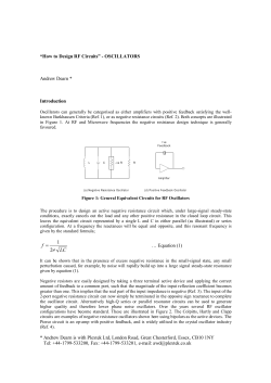
FIG. 1. A typical optomechanical system and the corresponding
spacetime diagram for the ingoing and outgoing light rays. Here
x,
ˆ aˆin and aˆout denote the oscillator position, ingoing and outgoing
fields, ωm , κm stand for oscillator frequency and decay rate, a,
ˆ κ and
L denote intracavity optical mode, cavity bandwidth and length, respectively. We assume bad cavity limit when κ ωm and thus the
dynamics of aˆ can be considered following the ingoing light adiabatically. For clarity, we intentionally place aˆin and aˆout on different
sides of the oscillator world line. The inclined lines represent the
light rays. Up to some instant we are concerned with (t = 0), the optical fields entering later are out of causal contact and thus irrelevant.
This paper is organised as follows: in Sec. II, we set our
model of optomechanical system and derive the dynamics
thereof; in Sec. III, we consider a conditional dynamics of
Gaussian mechanical states resulting from continuous monitoring of the outgoing light; in Sec. IV an entanglement between the outgoing light and mechanical oscillations of the
cavity mirror is studied in detail; Sec. V is devoted to the use
of the optomechanical entanglement for experimental demonstration of the quantum state steering; Sec. VI contains some
summarising remarks and concludes this paper.
The First International Workshop on Entangled Coherent States and Its Application to Quantum Information Science
— Towards Macroscopic Quantum Communications —
November 26-28, 2012, Tokyo, Japan
Stefan Danilishin et al.
10
II. OPTOMECHANICAL SYSTEM AND CONTINUOUS
MEASUREMENT
We start by considering a dynamics of a linear optomechanical device presented in Fig. 1 which has been extensively
studied [12, 18–20]; its linearised Hamiltonian reads:
ˆ aˆ† + a)
ˆ
Hˆ = pˆ2 /(2m) + mωm2 xˆ2 /2 + Hˆκm + h¯ Δaˆ† aˆ + h¯ gx(
√
†
†
ˆ .
(1)
+ i¯h κ (aˆext aˆ − aˆext a)
Here ωm is the mechanical resonant frequency; Δ = ωc − ωl
is cavity detuning, i.e., difference between the cavity resonant frequency ωc and the laser frequency ωl ; Hˆκm summarises the fluctuation-dissipation mechanism for the mechanical oscillator; the fifth term is the optomechanical interaction term with g ≡ a¯ ωc /L quantifying the coupling strength,
a¯ the steady-state amplitude of the cavity mode and L the cavity length; the last term describes the coupling between the
cavity mode and external continuous optical field aˆext with
[aˆext (t), aˆ†ext (t )] = δ (t −t ) in the Makovian limit and κ is the
coupling rate which is also the cavity bandwidth.
From Hamiltonian (1), one can obtain the following set of
linear Heisenberg equations of motion
˙ˆ + ωm2 x(t)]
¨ˆ + κm x(t)
ˆ
= Fˆrp (t) + Fˆth (t) ,
m[x(t)
√
˙ˆ + (κ /2 + i Δ)a(t)
a(t)
ˆ = −igx(t)
ˆ + κ aˆin (t) ,
(2)
(3)
and the input-output relation
√
aˆout (t) = −aˆin (t) + κ a(t)
ˆ ,
FIG. 2. The displacement noise spectrum of an optomechanical device and the characteristic frequencies of the force noise ΩF , the
quantum noise Ωq , and the sensing noise Ωx referring to the Standard Quantum Limit (SQL) in the strong measurement, bad-cavity
limit, i.e. when κ Ωq ωm .
(4)
where aˆin ≡ aˆext (t− ) (in-going) and aˆout ≡ aˆext (t+ ) (out-going)
are input and output operators in the standard input-output formalism [21], and Fˆrp ≡ −¯hg(aˆ + aˆ† ) is the quantum radiation
pressure force and Fˆth is the thermal fluctuation force associated with the mechanical damping. Output field aˆout can be
measured with a homodyne detection scheme, from which we
can infer the mechanical motion and thus the quantum state of
the oscillator. By adjusting the local oscillator phase, one can
measure any θ -quadrature: bˆ θ = bˆ 1 sin θ + bˆ 2 cos θ , which is
a linear combination of the output amplitude quadrature bˆ 1 ≡
ˆ 2 ≡ √1 (aˆout − aˆ†out ).
√1 (aˆout + aˆ† ) and phase quadrature b
out
2
2i
After incorporating non-unity photodetection efficiency η , the
measurement output at time t is given by
√ yˆθ (t) = η bˆ 1 (t) sin θ + bˆ 2 (t) cos θ + 1 − η nˆ θ (t) , (5)
where nˆ θ is the vacuum noise associated with the photodetection loss and is uncorrelated with aˆin . Note that θ can
be a function of time, when the local oscillator phase is adjusted during the measurement; in this way a different optical
quadrature (but only one) is measured at each moment of time.
Large cavity bandwidth and strong measurement limit.—
The particular scenario that allows for concise form expressions and at the same time represents all the physics is theone
when the cavity bandwidth is large and the optomechanical
coupling rate is strong — a strong measurement, compared
to the mechanical resonant frequency ωm . In this case, the
cavity mode can be adiabatically eliminated, and the mechanical resonant frequency ωm ignored (for general scenarios, the
formalism here still applies but the analytical results become
quite complicated). Correspondingly, equations of motion for
the oscillator read reads [cf. Eqs. (2) and (3)]:
¨ˆ = Fˆrp (t) + Fˆth (t) = −α aˆ1 (t) + Fˆth (t) ,
m x(t)
(6)
with aˆ1 ≡ √12 (aˆin + aˆ†in ) the amplitude quadrature of the input
field. The output amplitude quadrature yˆ1 and phase quadrature yˆ2 are given by [cf. Eqs. (4) and (5)]:
yˆ1 (t) =
yˆ2 (t) =
√
√
η aˆ1 (t) +
1 − η nˆ 1 (t) ,
η [aˆ2 (t) + (α /¯h) x(t)]
ˆ + 1 − η nˆ 2 (t) ,
(7)
(8)
where aˆ2 ≡ √12i (aˆin − aˆ†in ) is the phase quadrature of the input
field, and additionally we have introduced an effective coupling constant (measurement strength) α ≡ 8/κ h¯ g.
In this special case, all the noise sources are Markovian and
thus can be characterised by single values of their spectral
densities. However, it is instructive to introduce characteristic frequencies thereof, where displacement spectrums intersect the standard quantum limit (SQL) as a benchmark:
ΩF ≡ [2mκm kB T /(¯hm)]1/2 , Ωq ≡ [α 2 /(¯hm)]1/2 , and Ωx ≡
Ωq [2η /(1 − η )]1/2 . In Fig. 2, we plot these noise sources in
the strong measurement limit, when quantum fluctuations of
light dominate over all other noise sources in some frequency
band, set by the values of ΩF and Ωx . This is the general requirement one has to satisfy to be able to see quantum correlations, or use them for manipulations with mechanical quantum
states [10, 22].
The First International Workshop on Entangled Coherent States and Its Application to Quantum Information Science
— Towards Macroscopic Quantum Communications —
November 26-28, 2012, Tokyo, Japan
Proceedings of the First International Workshop on ECS and Its Application to QIS;T.M.Q.C., 9-18 (2013)
III. CONDITIONAL QUANTUM STATE.
Now suppose we perform homodyne detection during −τ ≤
t ≤ 0, obtaining a data string:
y θ = {yθ (−τ ), yθ (−τ + dt), · · · , yθ (−dt), yθ (0)}
(9)
with dt = τ /(N − 1) being the time increment and N the number of data points. We can then infer the quantum state of
mechanical oscillator at t = 0 conditional on these measurement data, obtaining the so-called conditional quantum state.
The standard way to obtain the conditional state is to use data
to drive the stochastic master equation [23–27]. Here we use a
different approach by using the Wigner quasi-probability distributions, deriving the conditional quantum state in a way
similar to classical Bayesian statistics, in the same spirit as the
approach applied in Ref. [22]; this allows us to more straightforwardly treat non-Markovianity, e.g., due to a small cavity
bandwidth and colored classical noises. Our approach takes
the advantage of the following facts:
ˆ
yˆθ (t)] = [ p(0),
ˆ
yˆθ (t)] = 0
[yˆθ (t), yˆθ (t )] = [x(0),
(10)
∀t,t ∈ [−τ , 0], which is a consequence of the general features of linear continuous quantum measurements [28]. We
can therefore treat yˆθ (t) almost as classical quantities and ignore their time-ordering in deriving the following joint Wigner
function of the oscillator and the continuous optical field:
W (xx, y θ ) = Tr[ρˆ (−τ )δ (2) (ˆx − x )δ (N) (ˆy θ − y θ )] .
(11)
Here we have only included the marginal distribution for the
optical quadrature yˆ θ of interests, instead of the entire optical phase space; xˆ ≡ (x(0),
ˆ
p(0))
ˆ
and x is a c-number vector,
similar for y θ ; ρˆ (−τ ) is the initial joint density matrix
ρˆ (−τ ) = ρˆ mth ⊗ |00
00|
(12)
with ρˆ mth the thermal state of the oscillator and |00
the vacuum
state for the optical field—the coherent amplitude of the laser
has been absorbed into the optomechanical coupling constant
g. Since x(0)
ˆ
and p(0)
ˆ
do not commute we have to explic
itly define δ (2) (ˆx − x ) = d 2 ξ e−iξ ·(ˆx −xx) . Similar to classical
Bayesian statistics, the Wigner function for the conditional
quantum state of the mechanical oscillator at t = 0 reads:
Wm (xx| y θ ) = W (xx, y θ )/W (yyθ ) .
(13)
Since we consider only Gaussian quantum states, the joint
Wigner function can thus be formally written as:
1
(14)
W (xx, y θ ) = c0 exp − (xx, y θ )Vθ−1 (xx, y θ )T ,
2
where c0 is the normalization factor and superscript T denotes
transpose. Elements of the covariance matrix Vθ are given by
Vθjk = Xˆ j Xˆ k sym ≡ Tr[ρˆ (−τ )(Xˆ j Xˆ k + Xˆ k Xˆ j )]/2
(15)
11
with Xˆ ≡ (ˆx , yˆ θ ). We separate components of the oscillator
and the optical field, and rewrite the covariance matrix V as:
A CT u Tθ
A CTθ
≡
.
(16)
Vθ =
Cθ Bθ
u θ C u θ BuuTθ
Here A is a 2×2 covariance matrix for the mechanical oscillator position x(0)
ˆ and momentum p(0);
ˆ
B is a 2N × 2N covariance matrix for two quadratures yˆ 1 ≡ yˆ θ =π /2 and yˆ 2 ≡ yˆ θ =0
of the optical field; u θ = (sin θ , cos θ ) is a N × 2N matrix
and sin θ ≡ diag[sin θ (−τ ), · · · , sin θ (0)]—a diagonal matrix
with elements being quadrature angle at different times; C is a
2N × 2 matrix describing the correlation between (ˆy 1 , yˆ 2 ) and
(x(0),
ˆ
p(0)).
ˆ
Combining Eqs. (13) and (16), we obtain:
1
1
|θ −1
exp − (xx − x |θ )Vm (xx − x |θ )T , (17)
Wm (xx| y θ ) =
π h¯
2
|θ
where the conditional mean x |θ and covariance matrix Vm are
T
x |θ = CTθ B−1
θ yθ ,
|θ
Vm = A − CTθ B−1
θ Cθ .
(18)
Note that the two rows of the 2N × 2 matrix, CTθ B−1
θ , which
we shall refer to as K x (the first row) and K p (the second
row), are also the optimal filters that predict x(0)
ˆ
and p(0)
ˆ
K p yˆ Tθ ]2 ,
K x yˆ Tθ ]2 and [ p(0)−K
ˆ
with minimum errors, [x(0)−K
ˆ
respectively. The above results for the conditional mean and
variance are formally identical to those obtained by classical
optimal filtering.
Continuous-time limit.—To properly describe the actual
continuous measurement process, we take the continuoustime limit with dt → 0, and we have N → ∞. The matrices
indexed by time become functions of time, while matrix products involving summing over time become integrals. In particular, the central problem of calculating K = CT B−1 becomes
solving an integral equation for K :
0
−τ
K (t ) = CT (t) .
dt B(t, t )K
(19)
More specifically, B(t, t ) now becomes a 2 × 2 matrix with
elements being the two-time correlation functions between
optical quadratures yˆ1 (t) and yˆ2 (t ); C(t)’s elements are corˆ
p(0)).
ˆ
relation functions between (yˆ1 (t), yˆ2 (t )) and (x(0),
These correlation functions can in turn be obtained by solving Heisenberg equations of motion [cf. Eqs. (2-5)] and exˆ
pressing x(0),
ˆ
p(0),
ˆ
yˆ1 (t), and yˆ2 (t) in terms of aˆin (t), n(t)
and Fˆth (t), for which we have aˆin (t)aˆ†in (t )
sym = δ (t −
ˆ n(t
ˆ )
sym = δ (t − t )/2 and Fˆth (t)Fˆth (t )
sym =
t )/2, n(t)
2mκm kB T δ (t − t ) given the initial state ρˆ (−τ ) shown in
Eq. (12). The above integral equation is generally difficult to
solve analytically if τ is finite. Since usually we are not interested in the transient dynamics, we can extend −τ to −∞,
which physically corresponds to waiting long enough till the
mechanical oscillator approaches a steady state, and then start
state preparation. In this case, Eq. (19) can be solved analytical using the Wiener-Hopf method of which the detail is
shown in the Appendix A.
The First International Workshop on Entangled Coherent States and Its Application to Quantum Information Science
— Towards Macroscopic Quantum Communications —
November 26-28, 2012, Tokyo, Japan
Stefan Danilishin et al.
12
IV. OPTOMECHANICAL UNIVERSAL ENTANGLEMENT
Now we can consider a problem of entanglement between
the mechanical oscillator and the outgoing light fields. Effectively, it is equivalent to bipartite enatanglement of a
single particle with N → ∞ other particles. According to
Refs. [29, 30], in order for one particle and a joint system of
arbitrarily large N particles to be separable, a necessary and
sufficient condition is that partially transposed density maT
trix ρ1|N1 (with respect to the first particle) should be positive
T
semidefinite, i.e. ρ1|N1 ≥ 0. In the phase space of continuous
Gaussian variables, this reduces to the Uncertainty Principle
Σ ≥ 0,
Vpt + iΣ
Σ=
N+1
k=1
0 1
σk where σk =
−1 0
(20)
FIG. 3. Logarithmic negativity EN as a function of the ratio Ωq /ΩF .
A mechanical quality factor Qm = 103 is chosen.
Qm ≡ ωm /(2κm ) 1, up to the leading order of 1/Qm , a very
elegant expression for EN is derived and it is
EN = (1/2) ln[1 + (25/8)Ω2q /Ω2F ].
(25)
Going for continuous time limit N → ∞, one can find λk by
solving eigenvalue problem [31]:
This expression clearly demonstrates that optomechanical entanglement persists at any temperature, as its measuer, the logarithmic negativity, depends only on the ratio of measurement
strength Ωq and thermal decoherence rate ΩF . In the previous
works on optomechanical entanglement [6, 8, 11], it depends
solely on decoherence rate ΩF . However, as we showed in
[12, 13], this is a consequence of disregarding the information that was carried out by the outgoing light and considering
only the entanglement between the intracavity optical mode
and the oscillator. When the continuum of the modes leaving
the cavity is properly accounted for, optomechanical entanglement turns out to be universal.
Let us now consider how long can this entanglement survive. After turning off the optomechanical coupling at t = 0,
the mechanical oscillator freely evolves for a finite duration
τ , driven only by thermal noise. Due to thermal decoherence, entanglement will gradually vanish. Mathematically, the
symplectic eigenvalue will become larger than unity when τ
is larger than the survival time τs . By replacing [x(0),
ˆ
p(0)]
ˆ
with [x(
ˆ τ ), p(
ˆ τ )] and making similar analysis, up to the leading order of 1/Qm , τs satisfies a transcendental equation:
4 Ω4F θs2 − (2 Ω2F + Ω2q )2 sin2 θs − 25 ωm4 = 0, with θs ≡ ωm τs .
In the case of Ωq > ΩF ωm , the oscillating term can be
neglected, leading to
Vpt v = i λ Σ v,
θs = (5/2)(ωm /ΩF )2 = 5 Qm /(2 n¯ th + 1),
Here we introduced a complete covariance matrix of the optomechanical system V ∈ R(2N+2,2N+2) as:
A CT
(21)
V≡
C B
and its partial transpose Vpt = T1 VT1 , where transformation
T1 = Diag[1, −1] ⊕ I2N , with I2N ∈ R(2N,2N) identity matrix,
performs a time inversion operation for a mechanical part of
which is equivalent to transthe system: Vpt = V| p(0)→−
ˆ
p(0)
ˆ
pose of mechanical sub-matrix in joint optomechanical density matrix ρ1|N [30].
According to the Williamson theorem, there exists a symplectic transformation S ∈ S p(2N+2,R) such that ST Vpt S =
N+1
T
k=1 Diag[λk , λk ]. Using the fact that S Σ S = Σ , the above
Uncertainty Principle reads λk ≥ 1. If this fails to be the case,
i.e. ∃ λk < 1, the states are entangled. The amount of entanglement can be quantified by the logarithmic negativity EN
[31] and
EN ≡ max[−∑k ln λk , 0] for k : λk < 1.
(22)
(23)
where v ≡ [α0 , β0 , |α ), |β )]T with | f ) denoting function of
time which belongs to L 2 [−∞, 0]. Due to uniqueness of |α )
and |β ) in terms of α0 and β0 for any λ < 1 (non-singular), Eq.
(23) leads to the following characteristic polynomial equation
det[A + iλ σk − CT (iλ σk + B)−1 C] = 0
(24)
Inversion of matrix iλ σk + B in continuous limit can be
done using the same Wiener-Hopf method discussed above
and presented in Appendix A. Solution shows, there is always one eigenvalue λ that is smaller than one and it only
depends on the ratio between Ωq and ΩF , which clearly indicates the universality of the quantum entanglement. In Fig.
3, the corresponding logarithmic negativity (c.f. Eq. (22))
is shown as a function of Ωq /ΩF . For a high-Q oscillator
(26)
where we have defined the thermal occupation number n¯ th
through kB T /(¯h ωm ) = n¯ th + (1/2). Therefore, in this case if
Qm is larger than nth , the entanglement will be able to survive
longer than one oscillation period. Since Qm > nth is also the
requirement that the thermal noise induces a momentum diffusion smaller than its zero-point uncertainty [28], this condition is what we intuitively expect. In the strong measurement
case with Ωq ΩF , the transcendental equation can be solved
numerically, showing that θs > 1 is always valid and the entanglement can survive at least up to one oscillation period.
It is evident from the above that optomechanical entanglement is a powerful resource for recovering macroscopic quantum correlations. In the next section we consider how it can be
used to demonstrate ”steering” of mechanical quantum state
by a different choice of measured quadrature of light.
The First International Workshop on Entangled Coherent States and Its Application to Quantum Information Science
— Towards Macroscopic Quantum Communications —
November 26-28, 2012, Tokyo, Japan
Proceedings of the First International Workshop on ECS and Its Application to QIS;T.M.Q.C., 9-18 (2013)
13
V. QUANTUM-STATE STEERING.
Optomechanical steering concept. — According to quantum mechanics, position and momentum of a mechanical oscillator satisfy the Heisenberg uncertainty principle, which
reads:
ΔXφ1 ΔXφ2 ≥ | sin(φ1 − φ2 )| ,
∀φ1 , φ2
(27)
where Xˆφ ≡ (x/Δx
ˆ
ˆ
q ) sin φ + ( p/Δp
q ) cos φ , with Δxq and
Δpq zero-point uncertainties in position and momentum, are
quadratures of the mechanical oscillator. Since the mechanical oscillator is interacting and establishing entanglement with
a continuous optical field, one can collapse it into desired
quantum state simply measuring continuously the outgoing
light with time-dependent homodyne angle θ (t) that defines
which optical quadrature is measured at time t. Suppose the
measurement lasts from −τ up to 0, the final conditional state
|θ
of the oscillator, written as |ψm (0)
, will depend on how we
make the homodyne detection due to entanglement. For two
different measurement strategies with θ1 (t) and θ2 (t), respectively, in general we have two different final conditional states:
|θ
|θ
|ψm 1 (0)
= |ψm 2 (0)
. If the quadratures are properly chosen,
we may have, as illustrated in Fig. 4:
|θ
|θ
ΔXφ11 ΔXφ22
< | sin(φ1 − φ2 )| ,
(28)
|θ
|θ
|θ
where ΔXφk k ≡ (Xˆφk − Xˆφk )2 1/2 with ·
≡ ψm k | · |ψm k .
In other words, if in the first strategy, the observer tries
to predict quadrature Xφ1 of the mechanical oscillator, while
in the second strategy, the observer tries to predict Xφ2 , then
the two predictions have an error product that is lower than
Heisenberg Uncertainty. The possible way to do it is summarised in Fig. 5.
In ideal linear quantum measurement processes, both conditional states will be pure, and for any pairs of distinctive
θ1 and θ2 , inequality (28) will almost always exist for some
set of φ1 and φ2 —although this idealised steerability may be
influenced by practical imperfections, such as thermal noise.
FIG. 5. Scheme of possible experimental setup (upper panel) and the
time chart of the experiment demonstrating optomechanical steering (lower panel). Here Alice, using two different measurement
strategies θ1,2 (t) (two time-dependent homodyne angles), prepares
many copies of two conditional states of the mechanical oscillator,
|θ
|θ
|ψm 1 (0)
and |ψm 2 (0)
, and passes the prepared states to Bob, also
providing him with sets of conditional estimates of position (xcnd (0))
and momentum (pcnd (0)) of the oscillator at time t = 0, which she derives at each instance of state preparation. Bob, using the same setup,
measures from t = 0 onwards, two different mechanical quadratures
of the oscillator, Xφ1 and Xφ2 , and reconstructs marginal probability distributions for these two quadratures. By calculating variances
|θ
|θ
ΔXφ1 1 and ΔXφ2 2 , he tests if Alice has succeeded in steering the mechanical state of the oscillator.
In view of Eq.(28), we introduce a figure of merit to quantify
steerability,
S ≡−
FIG. 4. (color online) Two different quantum states (projection
of their Wigner functions on phase space) of a mechanical oscillator, conditional on two different strategies for measuring the optical
quadrature: one at θ1 (t) (left) and the other at θ2 (t) (right).
⎧
⎨
min
φ1 ,φ2 ,θ1 ,θ2 ⎩
ln
⎫
|θ
|θ
ΔXφ11 ΔXφ22 ⎬
| sin(φ1 − φ2 )| ⎭
.
(29)
with minimum obtained by comparing all possible sets
of {φ1 , θ1 (t), φ2 , θ2 (t)} (t ∈ [−τ , 0])—an optimal timedependent homodyne detection is needed to achieve the lower
bound. The quantum state is steerable when S > 0, which
will be proved to be equivalent to the formal criterion obtained
by Wiseman for Gaussian entangled states [14].
As we will show in the discussion that follows, for linear
optomechanical devices, when the quantum radiation pressure
dominates strongly over thermal fluctuations, steerability only
depends on the photodetector efficiency η of time-dependent
The First International Workshop on Entangled Coherent States and Its Application to Quantum Information Science
— Towards Macroscopic Quantum Communications —
November 26-28, 2012, Tokyo, Japan
Stefan Danilishin et al.
14
homodyne detections:
S ≈
1
[ln η − ln(1 − η )] ,
2
(30)
which will be positive as long as η > 50%, which coincides
with the ideal limit shown by Wiseman and Gambetta [14].
Interestingly, such quantum steerability is intimately related
to the state tomography accuracy in the protocol suggested by
Miao et al. [32], in which an optimal time-dependent homodyne detection scheme is used to probe the quantum state of a
mechanical oscillator with Gaussian-distributed joint position
and momentum error less than Heisenberg uncertainty. More
explicitly, we will show, for the same optomechanical device,
(31)
S = − ln 2 det Vv /¯h ,
where Vv is the covariance matrix for the tomography error.
Theory of optomechanical steering. — We can now understand the quantum-state steering from a more quantitative
way. From Eq. (18), we learned that the conditional vari|θ
ance of the oscillator state Vm directly depends on the optical quadrature θ that we choose to measure. To calculate the
steerability figure of merit S [cf. Eq. (29)], we need to find
the time-dependent quadrature phase θ (t) that minimise the
|θ
conditional variance ΔXφ of a given mechanical quadrature
Xˆφ = v φ xˆ T with vector v φ ≡ (sin φ /Δxq , cos φ /Δpq ). Using
the fact that
|θ
min(ΔXφ )2 = minvvφ xˆ T − K yˆ Tθ 2
θ
θ,K
= min vvφ xˆ T − K 1 yˆ T1 − K 2 yˆ T2 2
K2
K 1 ,K
(32)
with K 1 ≡ K sin θ and K 2 ≡ K cos θ , we obtain the minimum
|θ
(ΔXφ )2min = v φ (A − CT B−1 C)vvTφ ,
and θ (tk ) at t = −τ + k dt is given by:
θ (tk ) = arctan (vvφ CT B−1 )k /(vvφ CT B−1 )N+k .
(33)
(34)
|θ
Since (ΔXφ )2min is in a quadratic form of v φ , we obtain:
S = − ln 2 det Vs /¯h ,
Vs ≡ A − CT B−1 C .
(35)
This means quantum state of the oscillator
is not steerable—
√
S < 0, if Vs is Heisenberg limited— det Vs > h¯ /2.
Such a definition of steerability is in accord with the criterion by Wiseman et al. [14], more specifically, shown in their
Eq. (17), which says that quantum state of the oscillator cannot be steered by the optical field, if we have
A CT
+ i Σm ⊕ 0o > 0 ,
(36)
C B
where Σ m ≡ σk is the 2×2 symplectic matrix for the oscillator,
and 0 o is a null 2N × 2N matrix for the optical field. Since the
covariance matrix B for the optical field is positive definite,
namely, B > 0, the above condition requires that the Schur’s
complement of A be positive definite:
A − CT B−1 C + i Σ m = Vs + i Σ m > 0 ,
(37)
which is equivalent to requiring that Vs is Heisenberg limited,
i.e.,
(38)
S = − ln 2 det Vs /¯h < 0 .
Large cavity bandwidth and strong measurement limit. —
Using the equations (7) and (8) and the definitions of Ωq ,
Ωx and ΩF thereafter, we can easily obtain those correlation
functions in the integral equation shown in Eq. (19). Using
Wiener-Hopf method of Appendix A, one can easily solve it
and get the following expression for Vs :
1
h¯ ζF
2 4 α 2 /(ζF h¯ m)
1
Vs = √
, (39)
3
2η
1
2 4 ζF h¯ m/α 2
where the characteristic constant ζF is defined as:
η
ζF ≡
2
1/2
4mκm kB T
.
1−η +
α2
(40)
Correspondingly, we obtain the steerability [cf. Eq. (35)]:
√
S = − ln 2 ζF /η .
(41)
For a strong measurement, the quantum radiation pressure
dominates over the thermal fluctuation force, and we have
rp
rp
SF = α 2 SFth = 4mκm kB T , with SF and SFth being the singlesided spectra density—twice the Fourier transform
of two
time correlation function. This leads to ζF ≈ η (1 − η )/2
and S ≈ 12 ln[η /(1 − η )], as shown in Eq. (30).
Connection between steering and quantum tomography.—
Interestingly, such quantum-state steering is closely related
to the quantum tomography protocol discussed in Ref. [32],
where an optimal time-dependent homodyne detection is proposed to minimise the error in obtaining marginal distributions of different mechanical quadratures, from which we reconstruct the Wigner function of the quantum state in phase
space. More specifically, for the same optomechanical device
discussed above, the tomography error—quantifying the difference between the reconstructed Wigner function and the
actual one—is given by the following covariance matrix:
1
h¯ ζF
2 4 α 2 /(ζF h¯ m)
−1
. (42)
Vv = √
3
2η
−1
2 4 ζF h¯ m/α 2
Notice that it is almost identical to the conditional covariance
matrix Vs shown in Eq. (39), apart from that the off-diagonal
terms have the opposite sign. The state steering can therefore be viewed as the time-reversal counterpart for state tomography, as the off-diagonal term flips sign when the oscillator momentum pˆ → − pˆ under t → −t, and the condition
for
√ achieving a sub-Heisenberg error for state tomography—
det Vv < h¯ /2, is also identical to that for steerability.
The First International Workshop on Entangled Coherent States and Its Application to Quantum Information Science
— Towards Macroscopic Quantum Communications —
November 26-28, 2012, Tokyo, Japan
Proceedings of the First International Workshop on ECS and Its Application to QIS;T.M.Q.C., 9-18 (2013)
15
below the SQL in order to prepare and verify quantum-state
steering. Noteworthy is the fact that steerability does not depend on the absolute value of the noise spectrum; one can
therefore have the flexibility to choose the appropriate frequency range to carry out the experiment, depending on the
specific setup.
The specific conditions for experimental demonstration of
steering that we formulated here are scalable to any experimental setup. As Fig. 6 clearly demonstrates, the experimentalist should have a system where quantum noise dominates
both thermal and sensing noise in a substantial frequency
range. The ratio of Ωx /ΩF 10 should be provided to see
steering in the experiment. Another important condition relates to
√ measurement strength that has to be of the order of
Ωq = Ωx ΩF . In terms of quantum noise it means that radiation pressure noise should dominate over thermal fluctuations.
FIG. 6.√Steerability Sv as a function of ratio Ωx /ΩF while keeping
Ωq = Ωx ΩF . Only the ratio between these frequencies determines
the steerability, and the absolute values can vary depending on the
chosen device.
Such a connection can be understood from the fact that for
steering, one tries to prepare states with minimal uncertainty
in certain quadratures Xˆφ (0) with data from (−∞, 0]—a filtering process, while for tomography, one tries to minimise the
error in estimating quadratures Xˆφ (0) with data from (0, ∞)—
a retrodiction process. Due to linearity, both the minimal uncertainty and the tomography error for a given quadrature Xˆφ
all takes the quadratic form—vvφ Vs, v v φT and
t → −t
Vs = A − CT B−1 C −−−−−→ Vv .
(43)
These two covariance matrixes Vs, v describe the remaining
uncertainty in oscillator position x(0)
ˆ
and momentum p(0)
ˆ
conditional on both the amplitude yˆ1 and phase quadrature yˆ2
of optical field, for t < 0 and t > 0, respectively. Note that the
above relation shown in Eq. (43) is exact only when the noise
during the state preparation and the one during tomography
are uncorrelated, as the correlation between them will break
down the time-reversal symmetry, which happens if the cavity
bandwidth is small and has noneligible memory time.
Verifiable steering and the experimental requirements. —
Not only are the steering and tomography intimately related
to each other, but also the tomography is necessary in order to
verify the steering in the experiment. For Gaussian states, the
tomography error simply adds on top of the covariance matrix
for every conditional state. We therefore define the following
figure of merit for verifiable quantum-state steering:
(44)
Sv = − ln 2 det[Vs + Vv ]/¯h = − ln(2ζF /η ).
We therefore require ζF < η /2 for verifing quantum-state
steering. It can be seen from comparing Fig. 2 and Fig. 6
that thermal noise from thermal fluctuation, and sensing noise
from optical loss and quantum inefficiency, need to be at least
VI. CONCLUSION
We see that quantum entanglement exists universally in system with a mechanical oscillator coupled to the continuum of
outgoing optical fields. The entanglement measure — logarithmic negativity displays an elegant scaling which depends
on the ratio between characteristic interaction and thermalnoise frequency. Such scaling should also apply in electromechanical systems whose dynamics are similar to what we have
considered. We also considered the possibility to use entanglement between light and mechanical motion for testing
such a fundamental concept of quantum mechanic as steering.
A close relation between steering and quantum state tomography procedure proposed in [32] is revealed. Our analysis
once again confirms a well-known condition that experimental demonstration of macroscopic quantum effects in optomechanical systems, including EPR-type entanglement, requires
the measurement apparatus to be quantum noise limited in
some frequency band of interest. Furthermore, the measurement has to be strong enough to effectively extract information about the mechanical motion at a rate higher than that
of a thermal decoherence which stipulates radiation pressure
noise to dominate over the thermal and sensing noise in this
frequency band. which is reflected in the relation between the
characteristic frequencies we introduced: ΩF < Ωq < Ωx .
ACKNOWLEDGMENTS
Authors would like to express deep gratitude to the organisers of the International Workshop on Entangled Coherent
State and its Application to Quantum Information Science and
Tamagawa University for the opportunity to present this work.
Special thanks to Prof. O. Hirota and Prof. T.S. Usuda for
kind invitation to share our research at this conference and
for all their support and hospitality. We also thank all the
members of the AEI-Caltech-MIT MQM group for fruitful
discussions. This research is supported by the Alexander von
Humboldt Foundation’s Sofja Kovalevskaja Programme, NSF
grants PHY-0956189 and PHY-1068881, the David and Bar-
The First International Workshop on Entangled Coherent States and Its Application to Quantum Information Science
— Towards Macroscopic Quantum Communications —
November 26-28, 2012, Tokyo, Japan
Stefan Danilishin et al.
16
bara Groce startup fund at Caltech, as well as the Institute for
Quantum Information and Matter, a Physics Frontier Center
with funding from the National Science Foundation and the
Gordon and Betty Moore Foundation.
Appendix A: Wiener-Hopf method
In this appendix, we show how to derive CT B−1 C in
Eq. (35), which is equivalent to solving an integral equation
shown in Eq. (19), with the Wiener-Hopf method. We first
show the general formalism and then specialise to the largebandwidth and strong-measurement limit that we have considered.
and [ f (ω )]+ is the part that is analytical in the lower-half
complex plane. From the definition of Fourier transform in
Eq. (A3), the inverse Fourier transform of [ f˜(ω )]− vanishes
for t > 0 from the residue theorem, namely
F −1 [ f˜(ω )]− = f (t)Θ(t) = 0 , ∀ t > 0 .
(A6)
Let us focus on the equations associated with the first col˜ i.e., j = 1 (the situation for j = 2 will be similar),
umn of C,
and we rewrite Eq. (A4) explicitly in terms of their components:
B˜ 11 (ω )K˜ 11 (ω ) + B˜ 12 (ω )K˜ 21 (ω ) − C˜11 (ω ) − = 0 , (A7)
B˜ 21 (ω )K˜ 11 (ω ) + B˜ 22 (ω )K˜ 21 (ω ) − C˜21 (ω ) = 0 . (A8)
−
Thirdly, if B11 (t) = B11 (−t), we can factorise B˜ 11 (ω ) as
B˜ 11 (ω ) = ϕ˜ + (ω )ϕ˜ − (ω )
1. General formalism
Here we first discuss the general formalism. In the
continuous-time limit, C is a 2 × 2 matrix with elements given
by Ci j (t) and, similarly, the elements of B are Bi j (t −t ) (i, j =
1, 2) and they only depend on time difference due to stationarity). We define K = B−1 C or equivalently, BK = C, and
K is a 2 × 2 matrix with the elements satisfying the following
integral equations:
2 0
∑
k=1 −∞
dt Bik (t − t )Kk j (t ) = Ci j (t) ,
(A1)
and therefore, inverting B is equivalent to solving the above
integral equation. Note that the upper limit of the integration
is 0, instead of +∞ in which case it can be solved simply by
using Fourier transform. This arises naturally in the classical
filtering problem with only past data that is available. The
procedure for using Wiener-Hopf method to solve this set of
integral equations goes as follows.
Firstly, we extend the definition of Ki j (t) and Ci j (t) to t > 0
but requiring Ki j (t) = Ci j (t) = 0 if t > 0, namely
Ki j (t) → Ki j (t)Θ(t),
Ci j (t) → Ci j (t)Θ(t) ,
(A2)
This allows to extend the upper limit of the integral to be +∞
without changing the result.
Secondly, we apply the Fourier transform
f˜(ω ) ≡ F[ f (t)] =
+∞
−∞
dt eiω t f (t) ,
of the above equation and obtain
2
∑ B˜ik (ω )K˜k j (ω ) − C˜i j (ω )
k=1
(A3)
= 0,
(A4)
−
where [ f (ω )]− means the part of f˜(ω ) that is analytical (no
poles) in the upper-half complex plane by using the following
decomposition:
f˜(ω ) ≡ [ f˜(ω )]+ + [ f˜(ω )]− ,
(A5)
(A9)
which is the Fourier counterpart of the Cholesky decomposition in time domain. We now can express K˜ 11 (ω ) in terms of
K˜ 21 (ω ) in Eq. (A7). We use the fact that
[ f˜(ω )]− = 0
=⇒
Multiplying Eq. (A7) by
[ f˜(ω )g˜+ (ω )]− = 0 , ∀g˜
ϕ+−1 (ω ),
we get
1 C˜11 B˜ 12 K˜ 21
K˜ 11 =
−
ϕ˜ − ϕ˜ +
ϕ˜ +
(A10)
−
.
(A11)
Plugging it into Eq. (A8), we obtain
B˜ 21 B˜ 12 ˜
B˜ 21 C˜11
K21 +
B˜ 22 −
ϕ˜ − ϕ˜ + −
B˜ 11
B˜ 21 B˜ 12 K˜ 21
+
− C˜21
=0
ϕ˜ −
ϕ+ +
−
where we have used the fact that:
B˜ 12 K˜ 21
B˜ 12 K˜ 21
B˜ 12 K˜ 21
=
+
.
ϕ˜ +
ϕ˜ + +
ϕ˜ + −
(A12)
(A13)
Again, if B˜ 22 − B˜ 21 B˜ 12 /B˜ 11 is an even function of time—
due to stationarity and time-reversal symmetry. We can make
a similar factorization to the one shown in Eq. (A9):
B˜ 21 (ω )B˜ 12 (ω )
B˜ 22 (ω ) −
= ψ˜ + (ω )ψ˜ − (ω ) .
B˜ 11 (ω )
(A14)
The same as the approach for deriving Eq. (A11) by using the
fact shown in Eq. (A10), we obtain
1
1
B˜ 21 C˜11
B˜ 21 B˜ 12 K˜ 21
C˜21 −
−
.
K˜ 21 =
ψ˜ − ψ˜ +
ϕ˜ − ϕ˜ + − ϕ˜ −
ϕ˜ + + −
(A15)
Note that in the above equation, K˜ 21 appears in both sides of
the equation, which might seems to be difficult to solve. Actually, since K˜ 21 is analytical in the upper half complex plane,
[B˜ 12 K˜ 21 /ϕ˜ + ]+ only depends on the value of K˜ 21 at the poles
of B˜ 12 /ϕ˜ + in the upper-half complex plane. One only need
to solve a set of simple algebra equations by evaluating the
above equation on these poles.
The First International Workshop on Entangled Coherent States and Its Application to Quantum Information Science
— Towards Macroscopic Quantum Communications —
November 26-28, 2012, Tokyo, Japan
Proceedings of the First International Workshop on ECS and Its Application to QIS;T.M.Q.C., 9-18 (2013)
2. Large-bandwidth and strong-measurement limit
In this section, we consider the case of the large-bandwidth
and strong-measurement limit, and, for the oscillator, we have
x(t)
ˆ =
t
−∞
p(t)
ˆ =m
dt Gx (t − t )[−α aˆ1 (t ) + Fˆth (t )] ,
t
−∞
dt G˙ x (t − t )[−α aˆ1 (t ) + Fˆth (t )] ,
(A16)
(A17)
yˆ2 (t) =
√
√
η aˆ1 (t) +
(A27)
(A28)
(A29)
(A30)
where
and, for the output optical field, we have
yˆ1 (t) =
and the correlation between (yˆ1 , yˆ2 ) and (x(0)
ˆ , p(0)):
ˆ
√
C˜11 (ω ) = − η α G˜ ∗x (ω ) ,
√
C˜12 (ω ) = −i mΩ ηα G˜ ∗x (ω ) ,
√ α
C˜21 (ω ) = η S˜xx (ω ) ,
h¯
√ α
˜
C22 (ω ) = i mΩ η S˜xx (ω ) ,
h¯
17
1 − η nˆ 1 (t) ,
η [aˆ2 (t) + (α /¯h) x(t)]
ˆ + 1 − η nˆ 2 (t) .
(A18)
(A19)
S˜xx (ω ) ≡ |G˜ x (ω )|2 (α 2 + 4mκm kB T ) ,
(A31)
and the Fourier transform for the mechanical Green’s function is given by [strong-measurement limit is taken by setting
κm , ωm → 0]:
G˜ x (ω ) =
Here
Gx (t) =
1 −κm t/2
e
sin ωmt
mωm
(A20)
is the Green’s function of the mechanical oscillator, and in the
strong-measurement limit—the frequency at which we carry
out the measurement is much higher than that of the mechanical frequency, the oscillator can be treated as a free mass and
Gx (t)|free mass = t/m.
By using the fact that
ϕ˜ + (ω ) = ϕ˜ − (ω ) = 1 ,
(A33)
For ψ˜ ± (ω ) [cf. Eq. (A14)], we have
α2 ˜2
|Gx (ω )|2 (1 − η )α 2 + 4mκm kB T
2
h¯
ω 4 + (κm2 − 2ωm2 )ω 2 + ωm4 + 2(α 2 /¯hm)2 ζF2
.
=
ω 4 + (κm2 − 2ωm2 )ω 2 + ωm4
(A34)
ψ˜ + (ω )ψ˜ − (ω ) = 1 + η
This leads to
Fˆth (t)Fˆth (t )
sym = 2mκm kB T δ (t − t ) ,
(A22)
we obtains the elements for covariance matrix B of (yˆ1 , yˆ2 ) in
the frequency domain (spectral density):
B˜ 11 (ω ) = 1 ,
(A23)
α2
G˜ ∗ (ω ) ,
h¯ x
α2
B˜ 21 (ω ) = −η G˜ x (ω ) ,
h¯
α2
B˜ 22 (ω ) = 1 + η 2 S˜xx (ω ) ,
h¯
B˜ 12 (ω ) = −η
(A32)
In this case, we can easily carry out the factorization. For
ϕ˜ ± (ω ) [cf. Eq. (A9)], we have
1
aˆ j (t)aˆk (t )
sym = nˆ j (t)nˆ k (t )
sym = δ jk δ (t − t ) (A21)
2
for j, k = 1, 2, and
−1
.
m(ω 2 − ωm2 + iκm ω )
(A24)
(A25)
ψ˜ + (ω ) = ψ˜ −∗ (ω ) =
[1] M. Aspelmeyer, P. Meystre, and K. Schwab, Physics Today
65, 29 (2012), URL http://link.aip.org/link/?PTO/
65/29/1.
[2] J. Chan, T. P. M. Alegre, A. H. Safavi-Naeini, J. T. Hill,
A. Krause, S. Groblacher, M. Aspelmeyer, and O. Painter, Nature 478, 89 (2011), ISSN 0028-0836, URL http://dx.doi.
org/10.1038/nature10461.
[3] A. D. O’Connell, M. Hofheinz, M. Ansmann, R. C. Bialczak,
M. Lenander, E. Lucero, M. Neeley, D. Sank, H. Wang, M. Wei-
(A35)
where ω j and ω j ( j = 1, 2) are the roots of the numerator and
denominator of Eq. (A34) in the upper-half complex plane, respectively. Given the expression for ϕ˜ ± and ψ˜ ± , we can solve
K˜ i j by using Eqs (A11), and Eq. (A15). This in turn allows us
to obtain Vs = A − CT K and in the time domain, it reads:
(Vs )i j = Ai j − ∑
k
(A26)
(ω − ω1 )(ω − ω2 )
,
(ω − ω1 )(ω − ω2 )
0
−∞
dt Cki (t )Kk j (t ) ,
(A36)
from which we obtain Eq. (39).
des, et al., Nature 464, 697 (2010), ISSN 0028-0836, URL
http://dx.doi.org/10.1038/nature08967.
[4] T. Purdy, R. Peterson, and R. C.A., arXiv:1209.6334 (2012),
URL http://arxiv.org/abs/1209.6334.
[5] A. Einstein, B. Podolsky, and N. Rosen, Phys. Rev. 47, 777
(1935).
[6] S. Mancini, V. Giovannetti, D. Vitali, and P. Tombesi, Phys.
Rev. Lett. 88, 120401 (2002), URL http://link.aps.org/
doi/10.1103/PhysRevLett.88.120401.
The First International Workshop on Entangled Coherent States and Its Application to Quantum Information Science
— Towards Macroscopic Quantum Communications —
November 26-28, 2012, Tokyo, Japan
Stefan Danilishin et al.
18
[7] M. Pinard, A. Dantan, D. Vitali, O. Arcizet, T. Briant, and
A. Heidmann, EPL (Europhysics Letters) 72, 747 (2005), URL
http://stacks.iop.org/0295-5075/72/i=5/a=747.
[8] D. Vitali, S. Gigan, A. Ferreira, H. R. B¨ohm, P. Tombesi,
A. Guerreiro, V. Vedral, A. Zeilinger, and M. Aspelmeyer, Phys.
Rev. Lett. 98, 030405 (2007), URL http://link.aps.org/
doi/10.1103/PhysRevLett.98.030405.
[9] M. Paternostro, D. Vitali, S. Gigan, M. S. Kim, C. Brukner,
J. Eisert, and M. Aspelmeyer, Phys. Rev. Lett. 99, 250401
(2007),
URL
http://link.aps.org/doi/10.1103/
PhysRevLett.99.250401.
[10] H. M¨uller-Ebhardt, H. Rehbein, R. Schnabel, K. Danzmann,
and Y. Chen, Phys. Rev. Lett. 100, 013601 (2008), URL
http://link.aps.org/doi/10.1103/PhysRevLett.100.
013601.
[11] M. J. Hartmann and M. B. Plenio, Phys. Rev. Lett.
101, 200503 (2008), URL http://link.aps.org/doi/10.
1103/PhysRevLett.101.200503.
[12] H. Miao, S. Danilishin, H. M¨uller-Ebhardt, and Y. Chen, New
Journal of Physics 12, 083032 (2010), URL http://stacks.
iop.org/1367-2630/12/i=8/a=083032.
[13] H. Miao, S. Danilishin, and Y. Chen, Phys. Rev. A 81, 052307
(2010), arXiv:0908.1053.
[14] H. M. Wiseman, S. J. Jones, and A. C. Doherty, Phys. Rev.
Lett. 98, 140402 (2007), URL http://link.aps.org/doi/
10.1103/PhysRevLett.98.140402.
[15] S. J. Jones, H. M. Wiseman, and A. C. Doherty, Phys. Rev.
A 76, 052116 (2007), URL http://link.aps.org/doi/10.
1103/PhysRevA.76.052116.
[16] D. J. Saunders, S. J. Jones, H. M. Wiseman, and G. J. Pryde, Nat
Phys 6, 845 (2010), URL http://dx.doi.org/10.1038/
nphys1766.
[17] H. M. Wiseman and J. M. Gambetta, Phys. Rev. Lett.
108, 220402 (2012), URL http://link.aps.org/doi/10.
1103/PhysRevLett.108.220402.
[18] F. Marquardt, J. P. Chen, A. A. Clerk, and S. M. Girvin, Phys.
Rev. Lett. 99, 093902 (2007), URL http://link.aps.org/
doi/10.1103/PhysRevLett.99.093902.
[19] I. Wilson-Rae, N. Nooshi, W. Zwerger, and T. J. Kippenberg,
[20]
[21]
[22]
[23]
[24]
[25]
[26]
[27]
[28]
[29]
[30]
[31]
[32]
Phys. Rev. Lett. 99, 093901 (2007), URL http://link.aps.
org/doi/10.1103/PhysRevLett.99.093901.
C. Genes, D. Vitali, P. Tombesi, S. Gigan, and M. Aspelmeyer,
Phys. Rev. A 77, 033804 (2008), URL http://link.aps.
org/doi/10.1103/PhysRevA.77.033804.
D. Walls and G. Milburn, Quantum optics (Springer, 2008).
H. M¨uller-Ebhardt, H. Rehbein, C. Li, Y. Mino, K. Somiya,
R. Schnabel, K. Danzmann, and Y. Chen, Physical Review
A (Atomic, Molecular, and Optical Physics) 80, 043802
(pages 18) (2009), URL http://link.aps.org/abstract/
PRA/v80/e043802.
A. Barchielli, International Journal of Theoretical Physics 32,
2221 (1993), ISSN 0020-7748, URL http://dx.doi.org/
10.1007/BF00672994.
G. J. Milburn, Quantum and Semiclassical Optics: Journal of
the European Optical Society Part B 8, 269 (1996), URL http:
//stacks.iop.org/1355-5111/8/i=1/a=019.
A. Hopkins, K. Jacobs, S. Habib, and K. Schwab, Phys. Rev.
B 68, 235328 (2003), URL http://link.aps.org/doi/10.
1103/PhysRevB.68.235328.
A. C. Doherty, S. M. Tan, A. S. Parkins, and D. F. Walls, Phys.
Rev. A 60, 2380 (1999), URL http://link.aps.org/doi/
10.1103/PhysRevA.60.2380.
A. C. Doherty and K. Jacobs, Phys. Rev. A 60, 2700 (1999),
URL
http://link.aps.org/doi/10.1103/PhysRevA.
60.2700.
V. Braginsky and F. Khalili, Quantum Measurement (Cambridge University Press, Cambridge, 1992).
R. F. Werner and M. M. Wolf, Phys. Rev. Lett. 86,
3658 (2001), URL http://link.aps.org/doi/10.1103/
PhysRevLett.86.3658.
G. Adesso and F. Illuminati, Journal of Physics A: Mathematical and Theoretical 40, 7821 (2007), URL http://stacks.
iop.org/1751-8121/40/i=28/a=S01.
G. Vidal and R. F. Werner, Phys. Rev. A 65, 032314 (2002),
URL
http://link.aps.org/doi/10.1103/PhysRevA.
65.032314.
H. Miao, S. Danilishin, H. M¨uller-Ebhardt, H. Rehbein,
K. Somiya, and Y. Chen, Phys. Rev. A 81, 012114 (2010).
The First International Workshop on Entangled Coherent States and Its Application to Quantum Information Science
— Towards Macroscopic Quantum Communications —
November 26-28, 2012, Tokyo, Japan