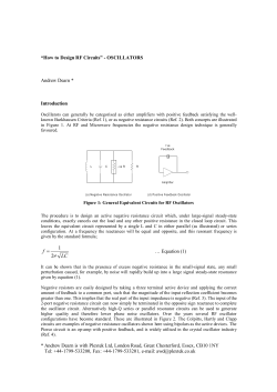
ELECTRONICS, VOL. 16, NO. 1, JUNE 2012
104
How To Measure Oscillator’s
Short-Term Stability Using Frequency Counter
Ivica Milanović, Snežana Renovica, Ivan Župunski, Mladen Banović, and Predrag Rakonjac
Abstract—In this paper a few methods of how to use frequency
counter in time-domain frequency stability analysis are
described. Three implemented methods are presented. As an
experiment, a comparison of the realized methods in the
Technical Test Center (TOC) and the “references” obtained in
the Directorate of Measures and Precious Metals (DMDM) in
Belgrade are accomplished. The measurement uncertainty
estimation for time interval measurement with one frequency
counter is presented as well.
Index Terms—Frequency, Frequency Counter, Oscillator,
Short-Term Stability.
F
I. INTRODUCTION
requency stability is one of the most important
specifications of an oscillator. Stability does not specify
how much frequency is accurate, but how much it is stable
during observed time interval. If considered time intervals up
to 100 seconds (10 ms, 100 ms, 1 s, etc.), then we talk about
so-called short-term stability. Otherwise, there is analysis of
long-term stability, and then we specify the oscillator’s
stability for an hour, and more often for a day, a month, or a
year [1].
Stability is defined as the statistical estimation of the
frequency or time fluctuations of a signal over a given time
interval. Statistical estimations can be presented in the
frequency or, more often, in the time domain [2]. To achieve
frequency stability in the time domain a set of a frequency
offset measurements have to be carried out, along with the
calculation of the collected data scattering.
II. THEORY OF FREQUENCY STABILITY MEASUREMENTS
nominal frequency and φ(t) is phase deviation.
In order to simplify further analysis, nominal voltage and
nominal frequency will be assumed as being constant. Also, it
is assumed that the amplitude deviation is negligible in
comparison with nominal voltage [3]. Due to that, the
instantaneous frequency is equal to:
1 dϕ
ν (t ) = ν 0 +
= ν 0 +νν
(2)
2π dt
and it is the sum of a constant nominal value ν0 and variable
term νυ(t).
We are not interested in large frequency deviations because
we are talking about reasonably stable oscillators. Therefore,
another restriction is:
(3)
νν (t ) << ν 0
The objective of the frequency stability analysis is to
characterize the phase and frequency oscillator fluctuations
with time [4]. In spite of that, we are primarily concerned with
the φ(t) term.
The aim is to determine the fractional frequency offset of
oscillator (device) under test (DUT) and reference oscillator:
1 dϕ
Δf ν (t ) − ν 0
(4)
=
= y (t )
=
f
2πν 0 dt
ν0
Measuring of frequency stability is a process which can be
divided into a few steps [3]:
− Preprocessing
− Collecting and storing data
− Outliers removal
− Noise type determination
− Data analysis (statistics)
− Results interpreting - reporting
Sine wave signal can be presented as:
V (t ) = [V0 + ε (t )] sin[2πν 0 t + ϕ (t )]
A. Preprocessing
Oscillator’s characteristics are highly dependent on
environment conditions, like a temperature change.
Preprocessing includes preparing and monitoring those
conditions, and monitoring the electrical power quality [3].
Manuscript received 18 December 2011. Received in revised form 14
March 2012. Accepted for publication 28 March 2012.
Ivica Milanović is with the Technical Test Center, Serbian Armed Forces,
Belgrade, Serbia (e-mail: [email protected]).
Snežana Renovica is with the Directorate of Measures and Precious
Metals, Belgrade, Serbia (e-mail: [email protected]).
Ivan Župunski is with the Faculty of Technical Science, University of Novi
Sad, Novi Sad, Serbia. (e-mail: [email protected]).
Mladen Banović and Predrag Rakonjac are with the Technical Test Center,
Serbian Armed Forces, Belgrade, Serbia (e-mail: [email protected]).
B. Acquisition
Frequency stability is observed over some period of time.
To determine it, we have to realize a set of frequency offset
measurements equally-spaced in time. The essential data is an
array of equally-spaced phase or frequency values taken at
particular measurement interval. Phase data are preferred,
because they can be used to obtain frequency data. This is not
(1)
where V0 is nominal voltage, ε(t) is amplitude deviation, ν0 is
DOI: 10.7251/ELS1216104M
ELECTRONICS, VOL. 16, NO. 1, JUNE 2012
always true if we want reverse analysis – absolute phase
cannot be reconstructed from frequency data, and all gaps in
frequency data will lead to loosing phase continuity [1]. In the
literature the sampling time or the measurement interval is
usually marked as τ0 [4]. The averaging time (τ) is a multiple
of the measurement interval (τ0):
τ = m ⋅τ 0
(5)
where m presents the averaging factor.
C. Outliers removal
System imperfection or some other external influences can
produce abnormalities in collected and stored data - some
values will significantly exceed expected quantities. Those
data are called outliers, and they have to be removed from the
collected array of data, before further analysis is carried out.
The median absolute deviation (MAD) is a robust way to set
the criteria for an outlier [3]. It is the median of the absolute
deviations of the data points from their median value (scaled),
and is defined as:
⎧⎪ y − m ⎫⎪
MAD = Median⎨ i
(6)
⎬
⎪⎩ 0.6745 ⎪⎭
where m is equal to Median{y(i)}. The factor 0.6745 makes
the MAD equal to the standard deviation for normally
distributed data.
An outlier criteria of 5·MAD [3] is usually a good choice.
Another, maybe more common way, is to use next criteria:
m + 3s < x( j ) < m − 3s
(7)
where x are data, j is number of data points, m is the mean
value of x, and s is the classical standard deviation of x.
D. Statistics – data evaluating
Frequency stability is a result of data taken in some period
of time, yet the independent variable is not the running time t,
but the averaging time τ. Regarding that, the experimental data
cannot be accurately described as a stationary process, so the
usual variances are not good way to express frequency
stability – the stationary concept means that observed process
has its beginning and its end. Limited time intervals of
observation are the main reason for inventing a new statistical
tool called Allan Variance [2].
It is developed in order to solve the problem that the
standard variance doesn’t converge to a single value for the
non-white FM noises as the number of measurements is
increased [1]. It is described as:
σ y2 (τ ) =
1
2( M − 1)
M −1
∑ (y
i +1
− yi
)
2
(8)
i =1
where σ is Allan Variation, τ is averaging time, M is number
of fractional frequency values, and yi is ith of M fractional
frequency data averaged over the τ.
While standard deviation subtracts the mean from each
measurement before squaring their summation, the Allan
deviation subtracts the previous data point. This differencing
of successive data points removes the time dependent noise
contributed by the frequency offset.
105
The stability is being improved as the averaging time (τ)
gets longer, because, in some cases, noises can be removed by
averaging [1]. However, on some level further averaging no
longer improves the results – that level is called the “noise
floor”.
The non-overlapping Allan, or two-sample variance, is the
standard time domain measure of frequency stability [3].
But, this kind of calculation can be performed by utilizing
all possible combinations of data sets. This is so-called
overlapping method [5]. It can be performed over the Standard
Allan Variation in order to improve the confidence of a
stability estimate:
σ y2 (τ ) =
1
2
2m ( M − 2m + 1)
M − 2 m +1 j + m −1
∑ ∑(y
j =1
i+m
− yi )
(9)
i= j
where σ is Overlapped Allan Variation, and m is averaging
factor.
Allan Variance can be described both tabular or in log-log
sigma-tau (σ-τ) diagrams. Those diagrams describe how much
we need to average in order to get rid of the noise contributed
by the reference and the measurement system.
There are several other variances which can be used, like
Modified Allan, Hadamard, Total, Time Variance etc.
However, Overlapping Allan Variance should be used as the
first choice [3].
E. Confidence Intervals
Sample variances are distributed according to:
χ2 =
edf ⋅ s 2
σ2
(10)
where χ2 is Chi-square probability, edf is Equivalent number
of Degrees of Freedom, s2 is the sample variance, and σ2 is the
true variance.
The edf depends of number on data samples and the noise
type. The lower and the upper bound of the sample variance
are:
edf
2
(11)
σ min
= 2
, (0 < p < 1)
χ ( p, edf )
edf
2
= 2
, (0 < p < 1)
(12)
σ max
χ (1 − p, edf )
where p is desired confidence factor.
F. Noise type determination
The instability of the most frequency sources can be
modeled by a combination of their frequency fluctuations
Sy(f). Measure of frequency stability versus the time over
which the frequency is averaged can be presented as:
Sy ( f ) ≈ f α
or
σ y (τ ) ≈ τ μ / 2
(13)
where Sy(f) is power spectral density, α is the parameter that
defines the noise model in a frequency domain, σy(τ) is
frequency stability vs averaging time, and µ is the parameter
that defines the noise model in a time domain, and it is equal
to µ = -α-1.
Some typical noises with α parameter values are shown in
Fig.1.
ELECTRONICS, VOL. 16, NO. 1, JUNE 2012
106
White Phase
α=2
Amplitude
Flicker Phase
α=1
White Frequency
α=0
Flicker Frequency
α=-1
curve, we can determine the dominant noise type of the
measured oscillator.
III. ELECTRONIC COUNTERS IN TIME INTERVAL
MEASUREMENTS
Frequency difference measurements can be carried out with
time interval counters – devices with two inputs (signal in one
input starts the measurement, and signal in second input stops
it). In this case we have a comparison between two signals:
the output signal from the reference oscillator and the output
signal from the oscillator under calibration (device under test
– DUT).
Random Walk Freq.
α=-2
Time
Fig. 1. Simulated Noises in the Time Domain.
White PN – usually exists as a result of signal amplifying,
and has no relation with resonance mechanism.
Flicker PN – it is related to resonance mechanism, and it is
usually made by noisy electronics.
White FN – it is a common type for passive resonator
frequency standards (cesium or rubidium). They contain slave
(usually quartz) oscillators whose frequency is “locked” to a
resonance feature of another device.
Flicker FN – its physical cause is typically related to the
physical resonance mechanism of an active oscillator,
electronics parts, or environmental properties. It is common in
high-quality oscillators, but it can be masked by white FN or
flicker PN in lower-quality oscillators.
Random Walk FN – it usually exists very close to the
carrier [6], and it is related to an oscillator’s physical
environment – mechanical shock, vibration, temperature, etc.
In a σ-τ diagram those simulations can be presented as in
Fig.2.
Fig. 2. Noises in the Time-Domain – σ-τ diagram.
So, if we calculate the slope of the derived Allan variation
Fig. 3. Using the time interval (or frequency) counter for frequency stability
measurements – basic idea.
This is the scheme which presents the basic idea of the
stability measurements [7]. A few methods are realized
according to that principle.
A. Reference oscillator
A measurement compares the DUT to a reference or
standard. The standard should have better short-term
characteristic – the test uncertainty ratio (TUR) should be
10:1, or even higher. When we talk about short-term stability,
the most common types of oscillators can be arranged in
ascending order: like the best quartz, then rubidium and then
the cesium commercial oscillators. Nowadays, the best
standards for short-term stability are so-called BVA quartz
oscillators (“Boitier a Vieillissement Ameliore”). For example,
Oscilloquartz BVA OCXO, type 8607 with option 15 (short
term option) has σ(τ) better than 1.5·10-13, for τ from 1 to 30
seconds.
B. Frequency counters
The frequency difference between DUT and standard is
detected by a time interval counter. Frequency counters are
most commonly used instruments with capabilities of the time
interval measuring. There are conventional counters,
reciprocal counters, counters with digital interpolation
scheme, etc. [8]. However, when we are talking about the time
interval measurements, a few characteristics of the counters
are dominant:
− Single-shot time interval resolution. It represents the
number of digits that counter can display. This
characteristic limits counter’s ability to measure frequency
offset, and determines the smallest frequency change that
can be detected without averaging,
ELECTRONICS, VOL. 16, NO. 1, JUNE 2012
− Accuracy in the time interval measurements,
− Dead time. It represents instrumentation delay between
successive measurements,
− Trigger level timing error,
− Trigger offset,
− Internal noises,
− Aging of the oscillator and its temperature changes,
− Asymmetry between channels (mismatch),
− Averaging capabilities, etc.
Some of those characteristics can be suppressed or even
overcome, and some of them cannot. The measuring
uncertainty calculation will show their effects on the shortterm stability measurements. This will be discussed later on in
a chapter VI.
C. Frequency dividers or frequency mixers
Most common output frequencies of oscillators are 5 MHz
or 10 MHz. Since they are not practical to measure with
frequency counters, frequency dividers or frequency mixers
are used to convert them to lower frequencies.
Despite the greater simplicity of the frequency dividers,
frequency mixers are more used [1]. They are more expensive,
require more hardware and additional oscillator, but they have
a much higher signal-to-noise ratio, and this is the main
reason for their usage.
D. Data logging
As a result, frequency counters give a set of frequency
offset measurements. Those data can be written to a paper, or
stored into some external memory space, in order to be
analyzed later.
In order to avoid extra usage of counter hardware resources,
and to suppress the measuring uncertainty and the dead time,
some external accumulators can be used. At the beginning,
analog plotters were used. They are changed with the
accumulators – while the dead time data are sent to the
accumulator’s memory. After the measurement, the data can
be read out later on. The main disadvantage is memory space.
Nowadays, the interfaces between the counters and personal
computers extend the capability to store data directly to PC
memory.
IV. REALIZED METHODS FOR SHORT-TERM STABILITY
MEASUREMENTS
Two methods are realized in Technical Test Center
laboratory: Direct time interval measurement and dual mixer
time difference method.
A. Direct time interval measurement method
In this method Hewlett Packard 5370A universal time
interval counter is used. It has good time interval resolution –
20 ps in a single-shot. Also, it has capability to work in a
binary mode of operation for time interval measurements –
minimum time between measurements is 165 µs instead of
330 µs (like in a normal mode). This way counter does not
perform any type of statistical measurement (mean, standard
107
deviation, etc.). Instead, counter outputs raw data – five binary
data form one decimal data (information of time interval
value).
HP 5370A is connected to a PC USB port with Agilent
GPIB/USB
interface.
Short-time
stability
82357A
measurement is automated with Agilent VEE Pro 7.0
software. Minimum sample time is 100 ms.
When the measurement is finished program transforms
binary data into decimal values, calculates Allan deviation and
draws σ-τ diagram. Frequency offset is calculated as:
Δf
Δt
=−
(14)
f
t
where Δt is time interval between two successive
measurements, t is averaging time, and Δf/f is the fractional
frequency offset.
Further data analysis is carried out with the AlaVar 5.2
software. It removes outliers (according to (7)), gives Allan
variation table results and charts, and can determine dominant
noise type (five noise types, as is described in the chapter IIF).
B. Dual mixer time difference method
This method is realized with: HP 5345A frequency counter,
two HP 10830A frequency mixers, HP 5358A accumulator (as
an additional plug in the HP 5345A), and HP 59308A timing
generator for HP 5345A external arming.
Trigger
Frequency counter
(HP 5345A + 5358A accumulator)
START
ARM
STOP
Timing generator
(HP 59308A)
Agilent VEE software
Agilent 82357A GPIB/USB
Frequency mixer
(HP 10830A)
IF
Frequency mixer
(HP 10830A)
LO RF
DUT
PC
(USB
port)
IF
LO RF
Power divider
Reference
oscillator
Difference oscillator
(Signal generator HP 8642B)
Fig. 4. Dual Mixer Time Difference Method with HP 5345A.
As a difference oscillator HP 8642B signal generator is
used. It provides νb= 6 kHz beat frequency (6 kHz sine wave
signal). External arming of HP 5345A is with 200 µs pulses
from HP 59308A.
The difference oscillator’s output (ν0±νb) is split by a power
divider, and applied to each mixer. Further measurement is
taken over 6 kHz IF signals.
To calculate σ(τ) formulas (15) and (16) are used:
ν
(15)
Δf i = b [(ti +1 − ti ) − (ti − ti −1 )]
τ
σ y (τ ) =
1
2N
N
∑
j =1
( Δf i ) 2
ν 02
(16)
where ti is time interval between 2 successive measurements,
ELECTRONICS, VOL. 16, NO. 1, JUNE 2012
108
νb is beat frequency, τ is averaging time, ν0 is nominal (carrier)
frequency, and N is number of samples.
This measuring method is also automated with Agilent VEE
Pro 7.0.
Because of the HP 5345A poor time interval measurement
resolution (2 ns), this method is also configured with HP
5370A frequency counter. The configuration is the same, but
timing generator was not used, because HP 5370A has no
capability of the external arming.
Frequency counter
(HP5370A in a binary TI mode)
START
STOP
Agilent VEE software
Agilent 82357A GPIB/USB
Frequency mixer
Frequency mixer
(HP 10830A)
IF
DUT
PC
(USB
port)
Symmetricom 5071A high performance cesium standard, in
DMDM`s time and frequency laboratory. This method was
assumed “reference”, which will be shown in the charts
below.
In Fig.6 the σ-τ diagram (Allan variance chart) for rubidium
oscillator stability is shown. It was compared with two
different quartz oscillators for 5 MHz outputs, measured with
HP 5370A (direct measurement). In the range from 0.1 to 4
seconds the difference between DMDM and TOC results is
significant. For τ=1s DMDM result is 5·10-12, and with direct
measurement 2·10-11. Nevertheless, as manufacturer specifies
Allan variance better than 5·10-11, the conclusion for the
averaging time 1s will not be wrong.
(HP 10830A)
LO RF
IF
LO RF
Power divider
Reference
oscillator
Difference oscillator
(Signal generator HP 8642B)
Fig. 5. Dual Mixer Time Difference Method with HP 5370A.
Three of these methods were compared with the “reference”
method realized in the Directorate of Measures and Precious
Metals. DMDM uses specially designed for time interval
analysis, TSC 5110A Time Interval Analyzer. It is designed to
measure the phase difference between two signals, to measure
frequency, to determine and draw Allan deviation and to draw
phase and frequency plots. Optionally, it can determine SSB
(single-sideband) phase noise.
This time interval analyzer is based on the heterodyne
method (method with two mixers), and uses intermediate
frequency (IF) of approximately 100 Hz (when equal
frequency oscillators are compared). The smallest sampling
interval is one period of the IF or 10 ms.
For the frequency standard DMDM uses Oscilloquartz
BVA OCXO 8607 (described in the chapter III-A), which is
one of the best commercial short-term stability standards.
Fig. 6. Direct method with HP5370A in a binary mode.
The same measurement was made using the cesium 3210.
The results are given in Fig.7. For τ = 1 s they are practically
the same. Still, under 1s difference is bigger as τ gets smaller.
V. EXPERIMENTAL RESULTS
Three different types of oscillators are used for short-term
stability measurements: HP 105B and HP 5061A quartz
oscillators, Racal Dana 9475 rubidium oscillator and
Oscilloquartz 3210 cesium frequency standard. They are
compared with three realized methods: with HP 5370A
universal time interval counter - direct method (in binary
mode of operation) and dual mixer method, and dual mixer
method with HP 5345A frequency counter.
The environmental conditions were 23°C±1°C, and
humidity 50%±10%.
In order to compare them, measurements are also taken
with TSC 5110A and frequency references BVA 8607 and the
Fig. 7. Direct method with HP5370A in binary mode.
As we introduced mixers in the measurements, the results
became better (Fig.8).
ELECTRONICS, VOL. 16, NO. 1, JUNE 2012
109
reliable results.
VI. MEASURING UNCERTAINTY
Regarding previous chapters it is obvious that counter’s
specifications are dominant in measuring uncertainty
contribution. All of those methods are based on time interval
measurements. Like an example, the measuring uncertainty
estimation for direct measurement with HP 5370A time
interval counter will be discussed.
A. Random Effects – Uncertainty Type A
The random effects vary in an unpredictable way each time
you make a measurement. They produce an unstable reading
on the counter’s display. This uncertainty is often assumed to
have an approximately normal distribution.
1. Resolution or Quantization uncertainty
Fig. 8. Use of HP5370A in binary mode – directly and with mixers.
Mixing 10 MHz with 6 kHz signal improves system
capabilities, especially in a band below 1 second.
In Fig. 9 we can clearly see the improvements made by
using time difference method, and with use of good standards.
This is uncertainty due to single-shot time interval
resolution of a counter [9]. For HP 5370A this resolution is
20 ps, and producer defines this uncertainty like:
±20 ps
δr =
± 2 ps
(17)
sample size
If we choose sample size 1, this contribution is ±22 ps.
2. Accuracy of a time interval measurement
Because of a great influence of jitter Hewlett Packard
defines uncertainty due to time interval measurement accuracy
as:
δ a = jitter
(18)
HP 5370A has typical jitter of 100 ps, so, total amount of
this contribution is ±100 ps.
3. Start/stop trigger point uncertainty due to noise
This uncertainty occurs when a time interval measurement
starts or stops too early or too late because of noise on the
input signal [9], as shown in Fig.10.
Fig. 9. HP 105B quartz oscillator stability measured with direct and dual
mixers methods – comparison.
Two quartz oscillators were compared (HP 105B and HP
5061A). The “worst” results were achieved with the direct
method.
Even the better counter was used (20 ps HP 5370A),
because of the lack of the timing generator, dual time
difference method realized with HP 5345A gave better results.
That shows the importance of the counter’s accurate arming.
The conclusion is that for oscillators with high short-term
stability, only dual time difference method can produce
Fig. 10. Start trigger points uncertainty due to noise.
There are two sources of the noise: noise on the signal
being measured and noise added to this signal by the counter’s
input circuitry:
ELECTRONICS, VOL. 16, NO. 1, JUNE 2012
110
Vni2 + Vne2
(19)
du
dt
where Vni is internal noise, Vne is external noise, and du/dt is
signal slew rate at trigger point.
The slew rate (du/dt) for sine-wave signal at the zerocrossing is:
du
= u ⋅ ω ⋅ cos(0) = 2 ⋅ π ⋅ f ⋅ U RMS ⋅ 2
(20)
dt
The internal noise for HP 5370A is 150 µV. If we assume
that input is 10 MHz sine-wave signal, with URMS =1 V, and
signal to noise ratio (SNR) 60 dB, formula (20) now is:
δ tn =
2
2
2
⎛ 150μV ⎞ ⎛ 1 ⎞
⎛ 150μV ⎞
2
⎜⎜
⎟⎟ + ⎜
⎟
⎟ + (0.001)
⎜
⎝ 1V ⎠
⎝ U RMS ⎠ ⎝ SNR ⎠
δ tn =
=
2 ⋅ π ⋅ f ⋅ U RMS ⋅ 2
2 ⋅ π ⋅ 10 MHz ⋅ 1V ⋅ 2
(21)
Finally, for start trigger point, measuring contribution is
±11 ps.
If we assume the same URMS for both signals at the counter
inputs, the uncertainty for stop trigger point will be the same
as for start trigger point, so we have δtn-start=δtn-stop= ± 11 ps.
B. Systematic Effects – Uncertainty Type B
Uncertainty type B is unchanged when a measurement is
repeated under the same conditions. Instead, those effects
cause an offset of the measurement result from the true value.
4. Start/stop trigger points uncertainty due to trigger level
offset or Trigger level timing uncertainty
This measuring uncertainty results from trigger level setting
uncertainty due to deviation of the actual trigger level from
the indicated, and from input amplifier hysteresis if the input
signals do not have equal slew rates [9][10].
2.5mV
(23)
2 ⋅ π ⋅ 10MHz ⋅ 1V ⋅ 2
As the input signals are equal we have:
δto-start=δto-stop= ± 28 ps
If we assume a rectangular distribution [10], the
corresponding standard uncertainty can be calculated by
δ to =
dividing by 3 , so we will have:
δto-start=δto-stop= ± 16 ps
5. Channel asymmetry uncertainty or Channel mismatch
uncertainty
This uncertainty is a result of unequal propagation delays in
the two counter’s inputs, and differences in rise times of the
input amplifiers.
Hewlett Packard for 5370A defines asymmetry better than
700 ps. Assuming a rectangular distribution this measuring
uncertainty contribution is δasymm= ± 404 ps.
6. Timebase uncertainty
This uncertainty is frequency deviation from it’s nominal
value (10 MHz in this example). HP 5370A uses external
reference from cesium frequency standard, so, the uncertainty
is the result of two main sources:
− aging of the oscillator (stability) – εa
(for Oscilloquartz 3210 Allan deviation for 0.1 s is: 1.3·10-11
for 2σ, or 0.65·10-11 for 1σ)
− temperature changes – εt
(for Oscilloquartz 3210 temperature changes are defined as:
2·10-12 in the range -5 °C to 55 °C)
The timebase uncertainty [9] is defined by:
δ TB = TI ⋅
ε a2 + ε t2
(24)
3
where TI is measured time interval (in this example it is
sampling interval of 100 ms), so, this contribution is:
δTB = ± 0.4 ps.
The influence of type A measuring uncertainty can be
reduced by averaging [5]. Experimental measurements are
realized within 90 s, 100 s, 180 s and 360 s, or 900, 1000,
1800, 3600 or 9000 samples, respectively. The summary
contribution of type A measuring uncertainty is calculated
using formula 25:
u RAND =
δ r2 + δ a2 + δ tn2 − start + δ tn2 − stop
= 3 ps
N
where N stands for the number of samples.
Finally, the expanded uncertainty for k=2 is equal to:
Fig. 11. Start trigger point uncertainty due to trigger level offset.
This uncertainty can be presented as:
ΔU
δ to =
(22)
du
dt
where ΔU is offset from zero.
For HP 5370A this offset from zero is less than 2.5 mV, so:
(25)
2
2
2
U (k = 2) = 2 ⋅ u RAND
+ δ to2 − start + δ to2 − stop + δ asymm
+ δ TB
(26)
U(k=2) = 0.809 ns
The influence of channel asymmetry is dominant one, and it
is shown that bigger averaging time does not result in
reducing measuring uncertainty.
In deciding which counter should be used, the user has to
pay particular attention on: channel asymmetry, accuracy of
ELECTRONICS, VOL. 16, NO. 1, JUNE 2012
the time interval measuring, and time base uncertainty of a
counter.
This way of estimating measuring uncertainty can be used
for all time interval measurements which are carried out with a
frequency counters.
VII. THE CONCLUSION
In this paper the oscillator’s short-term stability and
procedure of it’s measurement in the time domain was
described, in short. Particular phases of measurement, and the
way for a data analysis are given, too.
Three methods realized with frequency counter HP 5345A,
and time interval counter HP 5370A are described. The results
of real measurements are given in graphs. They are compared
with the results acquired in DMDM which are considered
referent ones. In the DMDM measurement was carried out
using the time interval analyzer with two standards: BVA
quartz oscillator and ultra stable cesium frequency standard.
The shot-term stability was measured for quartz oscillator HP
105B, rubidium frequency standard Racal Dana 9475 and
cesium frequency standard Oscilloquartz 3210.
The comparisons are presented in graphs. It is shown that
methods based upon the frequency counters can be used to
determine short-term stability for averaging time of one
second, or more. For smaller averaging intervals, more
reliable is method realized with time interval analyzers in
accordance with ultra stable oscillators like a references.
Direct measurements with counters are possible, but if we
want to improve measuring system capabilities, it is better to
compare IF frequencies, rather than their nominal values.
These methods can be realized either with dividers or
111
frequency mixers. Advantages and disadvantages are shown in
this paper.
The measurement of short-term stability is, basically,
measurement of time interval between two sinusoidal signals.
According to that, the measurement uncertainty estimation for
time interval measurement using frequency counter is given.
The analysis shows that the mismatch between counter
channels has the greatest influence to total measuring
uncertainty. For counters which are going to be used in
frequency stability measurements, this analysis shows what
are the most important characteristics we have to pay attention
on.
REFERENCES
[1]
[2]
M.A.Lombardi, “Fundamentals of Time and Frequency”, NIST, 2002.
P.Kartashoff, “Frequency and Time”, Monographs in Physical
Measurement, 1978.
[3] W.J.Riley, “Handbook of Frequency Stability Analysis”, Hamilton
Technical Services, July 2007.
[4] Rohde&Schwarz, “Time Domain Oscillator Stability Measurement Allan
Variance”, Application Note, Feb.2009.
[5] W.J.Riley, “The Averaging of Phase and Frequency Data”, Hamilton
Technical Services, Nov.2010.
[6] D.A.Howe, D.W.Allan, J.A.Barnes, “Properties of Oscillator Signals and
Measurement Method”, NIST
[7] Hewlett Packard, “Fundamentals of Time Interval Measurements”,
Application Note 200-3, June1997.
[8] Hewlett Packard, “Fundamentals of the Electronic Counters”,
Application Note 200, Mar.1997.
[9] Fluke, “Sources of Error in Time Interval Measurements”, Application
Note
[10] Pendulum Instruments, “Accurate Phase Calibration”, Application Note
CNT-81, AN-07