1. No category

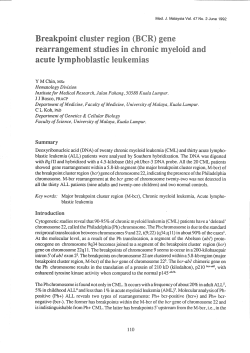
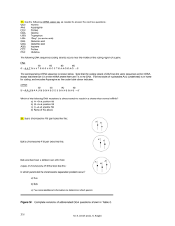
How to draw ideogram
Zuguang Gu <[email protected]>
German Cancer Research Center,
Heidelberg, Germany
July 5, 2013
The most widely use for the circos layout is to display genomic information. In most circumstances, figures contain an ideogram. Drawing ideogram
by circlize package is rather simple.
An ideogram is, in fact, a series of rectangles with different colors. In the
following example we are going to draw the ideogram for human.
The cytoband data for human can be download from
http://hgdownload.cse.ucsc.edu/goldenPath/hg19/database/cytoBand.txt.
gz. Uncompress the file and read it into R. Here the package already contains
such file.
> library(circlize)
> d = read.table(file = paste(system.file(package = "circlize"),
+
"/extdata/cytoBand.txt", sep=""),
+
colClasses = c("factor", "numeric", "numeric", "factor", "factor"))
> head(d)
1
2
3
4
5
6
V1
V2
V3
V4
V5
chr1
0 2300000 p36.33
gneg
chr1 2300000 5400000 p36.32 gpos25
chr1 5400000 7200000 p36.31
gneg
chr1 7200000 9200000 p36.23 gpos25
chr1 9200000 12700000 p36.22
gneg
chr1 12700000 16200000 p36.21 gpos50
In the data frame, the second column and the third column are intervals for
loci.
Here, setting the colClasses argument when reading the cytoband file is
very important, because the positions on chromosomes are large integers (the
second column and third column), read.table would store such data as integer
mode. The sumation of such large integers would throw error of data overflow.
So you must set the data mode to floating point (numeric).
Since chromosomes are sorted by their names which are as mode of character, the order would look like “chr1, chr10, chr11, ..., chr2, chr20, ...”. We need
to sort chromosomes by the numeric index first.
1
The process is simple. Extract the number part (1, 2, ..., 22) and the letter
part (X, Y) of chromosome names. Sorted them seperately and finally combine
them.
>
>
>
>
>
>
>
>
>
>
chromosome = levels(d[[1]])
chromosome.ind = gsub("chr", "", chromosome)
chromosome.num = grep("^\\d+$", chromosome.ind, value = TRUE)
chromosome.letter = chromosome.ind[!grepl("^\\d+$", chromosome.ind)]
chromosome.num = sort(as.numeric(chromosome.num))
chromosome.letter = sort(chromosome.letter)
chromosome.num = paste("chr", chromosome.num, sep = "")
chromosome.letter = paste("chr", chromosome.letter, sep = "")
chromosome = c(chromosome.num, chromosome.letter)
chromosome
[1] "chr1" "chr2" "chr3" "chr4" "chr5" "chr6" "chr7" "chr8" "chr9"
[10] "chr10" "chr11" "chr12" "chr13" "chr14" "chr15" "chr16" "chr17" "chr18"
[19] "chr19" "chr20" "chr21" "chr22" "chrX" "chrY"
The cytoband data also provides the range of each chromosome. This can
be set as the xlim of each chromosome. In the following code, we calculate the
start position and the end position of each chromosome and store them in a
matrix in which order of rows of xlim correspond to the order of elements in
chromosome.
By the way, if you don’t want to draw ideogram, reading the cytoband file
is also useful because it can help you to allocate chromosomes in the circle.
> xlim = matrix(nrow = 0, ncol = 2)
> for(chr in chromosome) {
+
d2 = d[d[[1]] == chr, ]
+
xlim = rbind(xlim,c(min(d2[[2]]), max(d2[[3]])))
+ }
Before we draw the circos layout, we need to set some graphic parameters.
Here we do not need any cell paddings and we also do not need the line width
to be too wide because genomic graph is a huge graph.
> par(mar = c(1, 1, 1, 1), lwd = 0.5)
> circos.par("cell.padding" = c(0, 0, 0, 0))
Initialize the circos layout with ranges of chromosomes. In the initialization
step, width of each sector would correspond to the range of each chromosome.
Also the order of sectors would be determined in this step. Here we must
explicitly set the levels of the factors to ensure the order of chromosomes is
“chr1, chr2, chr3, ...” or else the order would be the character order which is
“chr1, chr11, ...” (this is the default behavior for the function of factor). After
the initialization step, the position of each chromosome as well as the order are
2
stored in an internal variable. So in the later step, as long as the chromosome is
specified, graphs would be draw in the sector which corresponds to the selected
chromosome.
In the initialization step, order of the xim matrix should correspond to the
order of levels of the factors, so do not be confused here.
> circos.initialize(factors = factor(chromosome, levels = chromosome),
+
xlim = xlim)
After the range of each chromosome has been allocated in the circle, we can
draw the ideogram. Besides that, we also want to draw additional information
such as the axis for chromosomes and names of chromosomes. Here we would
draw ideogram, axis and the chromosome names in one track (It is just an option,
also you can draw ideogram, axis and names of chromosomes in different tracks).
in the following code, we create the first track in which there are 24 cells and
each cell corresponds to a chromosome. The x-range of each cell is the range of
the chromosome and the y-range of each cell is from 0 to 1.
> circos.trackPlotRegion(factors = chromosome, ylim = c(0, 1),
+
bg.border = NA, track.height = 0.1)
In the above codes, it is not necessary to set the factors argument. If
factors is not set, circos.trackPlotRegion will automatically create plotting regions for all available sectors which have already been initialized. But
explicitly specifying the factors argument would make your code more clear
for reading. And the value for factors does not need to be a real factor. If
it is not a factor, it would be converted to a factor internally. If the value for
factors is already a factor, the level of the factor also does not need to be
specified because the cells are positioned with the order of chromosomes which
is already defined in the initialization step.
Now in each cell, we draw the ideogram for each chromosome. Code is simple.
The steps are: for each chromosome, 1. assign different colors for different locus,
2. draw rectangle for different locus, 3. add axis, 4. add chromosome names.
Here the color panel is from http://circos.ca/tutorials/course/slides/
session-2.pdf, page 42.
> for(chr in chromosome) {
+
# data in `chr`
+
d2 = d[d[[1]] == chr, ]
+
n = nrow(d2)
+
+
# assign colors
+
col = rep("#FFFFFF", n)
+
col[d2[[5]] == "gpos100"]
+
col[d2[[5]] == "gpos"]
+
col[d2[[5]] == "gpos75"]
+
col[d2[[5]] == "gpos66"]
=
=
=
=
3
rgb(0, 0, 0, maxColorValue = 255)
rgb(0, 0, 0, maxColorValue = 255)
rgb(130, 130, 130, maxColorValue = 255)
rgb(160, 160, 160, maxColorValue = 255)
+
+
+
+
+
+
+
+
+
+
+
+
+
+
+
+
+
+
+
+
+
+
+
+
+
+
+
+ }
col[d2[[5]]
col[d2[[5]]
col[d2[[5]]
col[d2[[5]]
col[d2[[5]]
col[d2[[5]]
col[d2[[5]]
==
==
==
==
==
==
==
"gpos50"]
"gpos33"]
"gpos25"]
"gvar"]
"gneg"]
"acen"]
"stalk"]
=
=
=
=
=
=
=
rgb(200,
rgb(210,
rgb(200,
rgb(220,
rgb(255,
rgb(217,
rgb(100,
200, 200, maxColorValue
210, 210, maxColorValue
200, 200, maxColorValue
220, 220, maxColorValue
255, 255, maxColorValue
47, 39, maxColorValue =
127, 164, maxColorValue
= 255)
= 255)
= 255)
= 255)
= 255)
255)
= 255)
# rectangles for different locus
for(i in seq_len(n)) {
circos.rect(d2[i, 2], 0, d2[i, 3], 0.4, sector.index = chr,
col = col[i], border = NA)
}
# rectangle that cover the whole chromosome
circos.rect(d2[1, 2], 0, d2[n, 3], 0.4, sector.index = chr,
border = "black")
# axis
major.at = seq(0, 10^nchar(max(xlim[, 2])), by = 50000000)
circos.axis(h = 0.5, major.at = major.at,
labels = paste(major.at/1000000, "MB", sep = ""),
sector.index = chr, labels.cex = 0.3)
chr.xlim = get.cell.meta.data("xlim", sector.index = chr)
# chromosome names, only the number part or the letter part
circos.text(mean(chr.xlim), 1.2, labels = gsub("chr", "", chr),
sector.index = chr, cex = 0.8)
In the above code, you can find the ylim for the cells in the first track is
c(0, 1) and the y-value in circos.text is 1.2 which exceeds the ylim. There
may be some warnings saying some points are out of the plotting region. But
in fact it is OK to draw something outside the plotting regions. You just need
to ensure the final figure looks good.
If you do not want to draw ideogram in the most outside of the circos layout.
You can draw it in other tracks as you wish.
If there is a translocation from position 111111111 in chromosome 2 to position 55555555 in chromosome 16. It can represent as a link in the circos layout.
> circos.link(sector.index1 = "chr2", point1 = 111111111,
+
sector.index2 = "chr16", point2 = 55555555)
If position 88888888 in chromosome 6 is important and we want to mark it,
we can use following codes. First create a new track. Here there is no specifying
of factors, thus the new track would create plotting regions for all available
sectors (but with no borders. You would not see these cells but they really
4
14
13B
100
50MB
0MB
MB
15
0MB
100MB
50MB
100M
0MB
B
16
50MB
0MB
17
50M
B
50M
18
0M
B
50
M
B
12B
0M
B
MB
00
1
19
0M
B
50
M0
BM
M
50
0M
B
50
0M
B
50M
B
50MB
9
0MB
50MB
0MB
50MB
100MB
100MB
B
50M
1
150M
B
200
150
MB
B
M0BM
8
Y
100MB
0MB
150MB
0MB
B
100M
X
B
50M
100
MB
BB
0M
50M
10
22
B
0M
MB
10
B
21
B0M
11
M
50
0M
B
20
B
e
10
0M
B
M
15
15
0
2
0M
B
M
B0
B
50
MB
sit
50
7
0
10
B
MB
0M
MB
0M
20
M
B
10
0
B
MB
0M
50
B
50
MB
100
3
MB
B
150M
0MB
50MB
100MB
150MB
0MB
50M
B
100M
B
150
MB
0
6
MB
5
4
Figure 1: Ideogram in circos layout
exist.). Note you can not create plotting region for a single cell, however you
can write so, but in fact plotting region for cells in all sectors would be created.
>
>
>
+
>
+
# create a new track
circos.trackPlotRegion(ylim = c(0, 1), bg.border = NA)
circos.text(88888888, 0.2, labels = "site", sector.index = "chr6",
adj = c(0.5, 1))
circos.lines(c(88888888, 88888888), c(0.3, 1), sector.index = "chr6",
straight = TRUE)
The finnal figure looks like figure 1.
In the circlize package, there is already a circos.initializeWithIdeogram
function to initialize the circos layout with an ideogram. However, how to embed the ideogram into the circos layout is really subjective, such as the position
and colors of the ideogram, or maybe only subset of chromosomes are going
to be plotted, or maybe there are some zoomings for certain chromosomes (see
http://circos.ca/intro/features/. ‘GLOBAL AND LOCAL ZOOMING’
section). So the circos.initializeWithIdeogram is not a full functional function, it is only an example function to show how to allocate sectors for chromo5
50MB
0MB
50MB
B
50
0M
B
0M
0M
10
B
M
50
50
0M MB
B
gene
B
0M
e
MB
100
50M
B
0MB
100MB
50MB
0MB
100MB
gen
e
150M
B
ggeene
ne
100MB
50M
B
e
n
ge
MB
150
B
0M
ne
ne
nee
ggeen
MB
0M
0
10
MB
ne
ge
nee
ggeen
ge
gen
e
gen
ne
ge
gene
gene
gene
0M
B
0M
20
gene
gene
MB
0M
B
15
0M
B
15
B
0M
B
10
0M
gene
ge
ne
e
gen
e
e
ne
ne
gen
MB
ge
50
10
2
ggeene
ne
50
ge
ne
ge
ne
ne
B
ge
ge
200
ge
ne
ge
7
150MB
0MB
gene
MB
50
8
B
100M
gene
gene
gene
gene
gene
e
gen
gene
0M
B
10
11
e
ggeennee
n
geenee
g en e
g enne
gge ne
geennee
g e nee
g en e
gge n
e
ge en ne
g e
g
B
50M
1
gene
e
gen
e
ggeenne
B
50MB
0M
gene
gene
B
0M
gene
B
0M
Y
gene
gene
B
0M
X
gene
B
M
22
gene
50
21
gen
e
gen
e
gene
gene
ge
ne
gene
20
●
● ● ●●
● ●
●
● ●
●
● ●●
●
●
●
●
●
●● ●
● ●●
●●
●
●●●
● ●
●
●
●●
●●
● ●
●●
● ● ●● ●
●● ●
●
●● ●
●
●●
●●
●●
● ● ● ●●
● ● ● ●●●
●●
●●● ●
● ● ●●
●
●
● ● ● ●●
●●
●● ●
●● ●
●
●
●●●●
●
●
●
●
●●
●● ●
●
●●
●● ●●
●●●● ●
●● ●
●●●
●
●●●●
●
● ●
●●
●
●●●●
●
●●●●
● ●● ●
●●
●●
●
● ●●
●
●●
●
●●
● ●
●
●
●
●●
● ●● ● ●●
●
●●
●
●●
● ●● ●
●●
● ●●
●
●●●
●
● ●●●● ●
● ●
●
●●
●●● ● ● ●
●●
●
● ● ●●●●
●
●
●● ●●●
●
● ●
●●● ●●●
●●
●
●●●
●●
●●
●
●●
●●
●
●● ●● ●●
●
● ●
●
●● ● ●
●●●
●●●●
●
●
●
●
● ● ●●
●
● ●●
●
● ●●
● ●
●
●
●●●
●
●
●●
●● ●
●● ● ●● ●●
●
●
●
●●
● ●●
●
●
●● ●
●
●●●●●●●●
●● ●
●●●
●●
●●●● ● ●
●●
●●
●
● ●
●
●
●
●
●●
●
●●
●● ● ●
●●
●
●●
● ●●●●●
●
● ●● ●
●
●●
●
●
●●
●
●●●
● ●
●
●● ●
●●●●
●
●
●
●
●●●
●
●
●
●
●
●●
●● ●
●●
●● ●●●
●
●
● ● ●
●
●●
●
●●
●
● ●●
●
●●
●●● ● ● ● ●●●
●●●
●
●
●●●●
●● ● ●● ●●
●
●
●●
●●● ●
●●
● ●● ● ● ●
●● ●
●
●● ●
●
●● ●● ●
●
●
●●
●●
● ●● ● ● ● ●
●●
●●
●●
●
●●●
●
●
●
●
●
● ●●
●● ●
●
●
●●
●●
●●
●●
● ●●
●
● ●●
● ●●
●
● ●●●
● ●●●
● ●●● ●
●
● ●
●
●
●●●
● ●
●
●●
●
●
●
●
●
●●
●
●
●
●●●
●●
●
●
●
●
●●●
●
● ●●
●●
●
●
● ●
●
●
●
●
●● ●
● ●
● ●
●●
●
● ●● ● ●
●
● ●
● ●
●●
● ●
●●
●●● ●●●
●● ●
●
● ● ● ●●
●●●●
●
●
● ●●
●●
●●
● ●●●●● ● ●●●
●
●
●
●
● ●●
●
●
● ●
●
● ●
●
●
●
●
●
●● ● ●
●
●
●●●●
●
● ● ● ● ●●
●
●●
● ●●
●● ●
●●
●
●
●
● ●
●●
● ●●●
●●
●
●●
●
●●●
●
●
●
●
● ●
●●
●●
●●
●
●● ●
●●● ●
●
●
●●●
● ● ●
●
●●●
●
●
●
●●●
●
●●
●
● ●● ●●
●
●
●
●
●
●
● ●
●● ● ●
● ● ●●
●● ●
●
●●●
●●
●●
●●● ●●●
● ●●
●
●
● ● ●●●●●
● ●●
●●
●
●
●●
●●●
●
●
●
●●
●
● ●
●
●
●
●
●●
●●
●●
●
●●
● ●● ●
● ●●
●
●
●●
●
●
● ● ●
●●
● ●
●
● ●
● ●
●
●●●●
●
●
●
●● ●
●● ● ●
●●● ●●
●●
●● ●
● ●●
●
●
●●●
●●
● ●●
●
●
●
●
●
●
●●
●
●
●●●●●
●
●
●●
●● ●●
● ●
●●
●●
●
●● ●
●
●●
● ●●●
●●
●
●●
●
● ●●
●
●
● ●●
●
●
●●
●
● ●
●
● ●● ●
●● ●
●● ●
● ●●●
●● ●● ●
●
●
● ● ●● ●●
●
●
●
●●
● ●
●
● ●● ●● ●
● ●●
●● ● ●
●
●●
●
●●
●
●
●
●
●●
●
●
●●
● ●●
●
●
●●
●● ●
●● ●● ●
●●●
●
●
●
●
●
●
●●
●
●●●●
● ●●●●●●
●
●● ●
● ●
●
● ●
● ●●
●● ●●● ●
●●
●
●
● ●
●●
● ●
●
●● ● ●●
●●
●●
●●
●
●
●●
●
●
●●
●
● ●●
●●
● ●
● ●●● ●
● ● ●
●
●
●
●
●● ●
●
●
●
●● ● ● ● ●
●
●
●
●● ● ●● ●
●
●
●●
●
●
●
●
● ●
●
● ●● ● ●
● ●● ●●
●
●●
● ●●
●●
●
●
●●
●
● ●● ●●
●
●
●
●
●●
● ●●
●●
●
● ●●● ●
●●●●
●● ●
●● ● ● ●
●●● ● ●●
●
●
● ●
●
●
●●●
●
●
● ●
●● ●
●
●●
●● ● ●●
●●
●
●●
●
●
●
● ●
●
●
●
●
●
●●
●●
●●●
●●
● ● ●●
●
●●
●● ●
●
● ●●
●
●
●
●
●●
●
●●● ● ● ●
● ●
●●
●
●●
● ●
●
●
● ● ●●
● ●●●
●●
●
● ●● ●
●● ● ●●
●
●
●
●●
●●●● ●●●
●
● ●●
●
● ●●
● ● ● ●●
●
● ●
●● ● ● ● ●
● ● ● ●● ●
●
●
●
●
●
●
● ●
●
●
●
●
●●●●
●●
●
●●
●
●
●●
● ●
●
● ●
● ●
●
●
● ●●
● ● ●●
●
●
● ●
●
●
●●
●●●
●● ● ●
● ● ●●●●
●●
●
●
● ●
●● ●
●
●
●
●●●●
● ● ●●● ●
●●
●
●●
●●
●
●●● ● ● ●
● ●● ●
●● ●
●●● ●
●
●
●
●
●
●
●
●
● ●●
● ●
●
●
●
●●
● ● ● ●●●
●
●
● ● ● ●●
● ●●
●
●●
●
● ●●
●●
●●●
● ● ●
●●
●●● ● ● ●
● ●
●●●
● ●
●●●
●
●
●●
●●●
● ●●
●
● ●
● ●●
● ●●● ●
●●
●● ●
●
●●
●
●
● ●●
● ●●
●●
●●
●
● ● ●
●●
●
●
●●
● ● ● ●●
●
●
● ●●
●● ● ●
●
●
● ●●●
●
●●● ●●●
●
●
●●●
● ●● ●
●
●●●●
●●●
● ● ●●
● ●
●
●
●
●●
●
● ●
●
●
●● ●● ●
●●
●
●●
● ●●
●● ● ●●
●
●
●●
●
●● ●
●
●
●●
● ●● ●
●
● ● ●●● ●
●
●● ●
●
●●
●● ● ●
● ●
●●
●
●
●
●●
●
● ●●
●
●
●
●●
●
●● ● ●
● ●
●
●
●●
●●● ● ●●
● ●
●
●●
●
● ●
● ●●
●
●
●
●
●
●
●
●
●
●
●
● ●
●
●●
●
●
●
●
●
●●
●
● ●
●
●●
●
●
●
●
●●
●
●
● ●
●
● ● ●
●
●
●
●
●● ●●
●
●●●
●
●
●●
●
●
●
●●●● ●
● ●●● ●
●
●
●
●
●● ●● ●●●● ●
●
●●●
●●
●
●
●
●●●●● ● ●
● ● ●
●
● ●●
●
●
●●
●
●
●
●●
●
●●
●
●●●●●●
●● ● ●●
●●
●
●
●●
● ●
●
●
●●● ●
● ●●
● ●●
●
●
●
● ●
●
●● ●
●●
●
● ●
●
● ● ● ●●●●
●●
● ●
●●
● ●
●●
●
●●●
●
●●●
●
●●
●
●●
●
●
●
●● ●●●●
●● ●●● ●●●
●
● ●●● ● ●
●
●●
●
● ●
●●
● ●
●
●
●
●
●
●
●
●
●
●
●
●●●●
● ●●
● ●
●●
●● ● ●● ●
●● ●
●
●●●
●
●●
●
●●
● ● ●●●
●
●
●
●
● ● ●
●
●
●● ● ●
●
●
●
●
●
● ● ●● ●
●
●
●
●●
●●
●● ● ●
●● ●●●
● ●●
●● ● ●
●●
●
●
●
●●
● ●●
●●
●
● ●●●
●
●● ● ●● ●
● ●● ● ●●
●●
●
●●● ●
●
●●● ●
●
●
●
●
●
●
●
●
●
●
●
● ●●
●●
●
● ●
● ●
●●● ●
●●
●●
●● ● ●
●
●●
●
●
●●
●●
●
● ●
●
●●
●
● ●● ●
●
●
●● ●
●●●
●
●● ● ●
●
●●● ●●
●
● ●
●
●
●●●
●●
●
●
●● ●
●
●
●●
●
●●● ●
●
●
●
●●
●
● ●●
●● ●
●
●●
●● ●
●●●●●
●
●
●●
● ●
●
●
●● ●
●
●● ●
●
●
●●
●●● ●●
●●● ● ● ●
●
●
●● ● ● ●
●●
●
●
●
●●●
●● ●
●●
● ●● ●●●●●
●●
●●
●
● ●
●● ●
● ●●
●●
●
●●
● ●●●● ●
●●
●●
●●
●●●●
●●● ●●
●
●
●
●
●● ● ●●●
●
●●
●●
●●●● ● ● ●●
●● ●●
●●
●●
●
●
●●●
●●● ●
●
●●● ●
●
●
●● ●● ●
● ●●●
●
●●
●●
●●●
●●
●
● ●●
●●
●●
● ●●
● ● ●●
●
●
● ●
●●
●● ●
●●
●
●
●
●
●
● ●●
●
●
●
●●
●
● ●●
●●
●
● ●
●
●●
●
● ●
● ●
●
●●
●● ● ●
●
●
●●●●●
● ●● ●
● ●
●● ●
●
●
●●●●
●●● ●
●
●
●
●
●
●
●●● ● ●
●
●
● ●●●●
●●
●●●
●
●
●●
●
●● ●●●
●
●● ● ● ●
●
●● ●
●● ●
●● ●
●● ●
● ● ●●
●
●●
●
●●
●
●●
● ●
●
● ●
●
●●
●●
● ●
●
●
● ● ●●
●
●
●●
● ● ●●
●●
●
●●
● ●●
●●
●
●●
●●
●●●
●●●
●●
●
● ● ●
● ● ● ●● ●
●
●● ●●●
●
●
●
●●
●
●
●● ●
●
● ●
●●
●●
●
●
●
●●
●●●● ●
●●
●
●
●
●
●●
● ●●●
● ●●●
●
●
● ●●●●●●●
●
● ● ●●
● ●●
● ●●
●
● ●●
●
● ● ●
●
●
● ●●
● ●
●
●
●
●●
● ●●
●●
●●
●
●●
●
●
● ●●
●● ●
●●
●
●● ●
●
●
●
●
● ● ●●
● ● ●●
●●
● ●
●●●
●●●
●●●●
●● ●
●●●●●●
●● ●●
●●●
●
●
●
● ●
● ●●
●
●
●
●● ●
●● ●
● ●●
● ●
●● ●●●●● ●●●
●
●●
● ●●
●●
●
●
●●
●●
●
●●
●● ●●●● ●●
●
●
●
●●
●●●●
●●●
●
●●● ●● ●
●●
●
●●
●
●●●●
●
●
● ●●
● ●●
●●
●
●
●●●●
●
●
● ●● ●
●●
●
●●
●
●
●●
●●●●
●
● ●●
●●
● ●
●
●●
●
●
●● ●
● ●●
●● ●
●
●● ●
●
●●
●●●
●
●
●
●
●
●● ●●
●
● ●
● ● ● ● ●●
● ● ● ●●
●
● ● ● ● ●● ● ●●
●●
●● ●
●●
●●
● ● ● ●
●●●
●
●● ● ●
● ● ●
● ● ● ● ●● ●
● ●●
●
●
● ● ●●
●
●
●
● ● ● ●● ●
●●
●
●●●● ●
●●●●
●
● ●
● ●●
●
●
ggeen
ne
ge e
n
ge e
ne
ge
ne
ggeenne
e
9
19
gge
g en
g e nee
ge enene
ggeenne
ge nee
ge ne
ge ne
ne
ggeene
genne
gen e
gen e
genee
ge
ne
gene
gene
gene
gene
gen
e
gene
gene
gene
e
gen
gene
gene
gene
gene
e
genne
e
g
e
gen
e
gen
ne
ge
ne
ggeene
ne
ge e
n
ge
ne
ge
10
18
gen
12
MB
50M
B
17
0M
B
50MB
16
0MB
50MB
100MB
0MB
100MB
0MB
50MB
0MB
B
15
B
50M
14
MB
100
13
B
50
M
0M
50
MB
100
3
MB
B
0MB
150M
100MB
50MB
4
150MB
0MB
6
5
B
50M
B
100M
MB
150
B
0M
B
B
Figure 2: Detailed genomic graph
somes and how to draw ideogram. Thus users can draw their style of ideogram
according the above example codes. All you need to remember is that complicated graphs are assembled by simple graphs.
Finally, more informative and specialized genomic graphs are figure 2 and
figure 3. Figure 3 in fact combines two independent circos plots, users can refer
to the main vignette to find out how to realize it.
6
ch
r
19
0M
20
B
0M
B
chr1
B
B
chrX
220
30M
B
MB
230M
20MB
B
chrY
240MB
10MB
chr9
0
r2
ch 21
r
ch
r22
ch
0M
21
B
0M
B
18
MB
17
0M
MB
160
B
150
B
B
M
70
MB
M
B
40
M
140MB
120MB
130MB
MB
100
80
90M
60
50
M
110MB
11
chr1
0
19
ch
r
18
chr
17
chr16
chr15
chr14
13
chr
12
r
ch
ch
r
0MB
chr1
chr8
7
r
ch
ch
r
3
chr
chr4
chr
5
ch
r6
2
Figure 3: Two tracks of chromosomes in which the inner one zooms in chromosome 1 from the outer one.
7