
How to Value Bonds and Stocks EXECUTIVE SUMMARY
How to Value Bonds
and Stocks
EXECUTIVE SUMMARY
he previous chapter discussed the mathematics of compounding, discounting, and
present value. We also showed how to value a firm. We now use the mathematics of
compounding and discounting to determine the present values of financial obligations of the firm, beginning with a discussion of how bonds are valued. Since the future cash
flows of bonds are known, application of net-present-value techniques is fairly straightforward. The uncertainty of future cash flows makes the pricing of stocks according to NPV
more difficult.
5.1 DEFINITION AND EXAMPLE OF A BOND
A bond is a certificate showing that a borrower owes a specified sum. In order to repay the
money, the borrower has agreed to make interest and principal payments on designated
dates. For example, imagine that Kreuger Enterprises just issued 100,000 bonds for $1,000
each, where the bonds have a coupon rate of 5 percent and a maturity of two years. Interest
on the bonds is to be paid yearly. This means that:
1. $100 million (100,000 X $1,000) has been borrowed by the firm.
2. The firm must pay interest of $5 million (5% X $100 million) at the end of one year.
3. The firm must pay both $5 million of interest and $100 million of principal at the end of
two years.
We now consider how to value a few different types of bonds.
5.2 How TO VALUE BONDS
Pure Discount Bonds
The pure discount bond is perhaps the simplest kind of bond. It promises a single payment,
say $1, at a fixed future date. If the payment is one year from now, it is called a one-year discount bond; if it is two years from now, it is called a two-year discount bond, and so on. The
date when the issuer of the bond makes the last payment is called the maturity date of the
bond, or just its maturity for short. The bond is said to mature or expire on the date of its final payment. The payment at maturity ($1 in this example) is termed the bond's face value.
Pure discount bonds are often called zero-coupon bonds or zeros to emphasize the fact
that the holder receives no cash payments until maturity. We will use the terms zero, bullet,
and discount interchangeably to refer to bonds that pay no coupons.
Material reproducido por fines académicos, prohibida su reproducción sin la autorización de los titulares de los derechos.
ChapterS
How U) Value Bonds and Stocks
• FIGURE 5.1
103
Different Types of Bonds: C, Coupon Paid Every
6 Months; F, Face Value at Year 4 (maturity for pure
discount and coupon bonds)
Months
Pure discount bonds
Coupon bonds
Consols
The first row of Figure 5.1 shows the pattern of cash flows from a four-year pure discount bond. Note that the face value, F, is paid when the bond expires in the 48th month.
There are no payments of either interest or principal prior to this date.
In the previous chapter, we indicated that one discounts a future cash flow to determine
its present value. The present value of a pure discount bond can easily be determined by the
techniques of the previous chapter. For short, we sometimes speak of the value of a bond
instead of its present value.
Consider a pure discount bond that pays a face value of F in T years, where the interest
rate is r in each of the T years. (We also refer to this rate as the market interest rate.) Because
the face value is the only cash flow that the bond pays, the present value of this face amount is
Value of a Pure Discount Bond:
The present value formula can produce some surprising results. Suppose that the interest rate is 10 percent. Consider a bond with a face value of $1 million that matures in 20
years. Applying the formula to this bond, its PV is given by
or only about 15 percent of the face value.
Level'Coupon Bonds
Many bonds, however, are not of the simple, pure discount variety. Typical bonds issued by
either governments or corporations offer cash payments not just at maturity, but also at regular times in between. For example, payments on U.S. government issues and American
corporate bonds are made every six months until the bond matures. These payments are
called the coupons of the bond. The middle row of Figure 5.1 illustrates the case of a fouryear, level-coupon bond: The coupon, C, is paid every six months and is the same throughout the life of the bond.
Note that the face value of the bond, F, is paid at maturity (end of year 4). F is sometimes called the principal or the denomination. Bonds issued in the United States typically
have face values of $1,000, though this can vary with the type of bond.
Material reproducido por fines académicos, prohibida su reproducción sin la autorización de los titulares de los derechos.
104
Pan II
Value and Capital Budgeting
As we mentioned before, the value of a bond is simply the present value of its cash
flows. Therefore, the value of a level-coupon bond is merely the present value of its stream
of coupon payments plus the present value of its repayment of principal. Because a levelcoupon bond is just an annuity of C each period, together with a payment at maturity of
$1,000, the value of a level-coupon bond is
Value of a Level-Couoon Bond:
where C is the coupon and the face value, F, is $ 1,000. The value of the bond can be rewritten as
Value of a Level-Coupon Bond:
As mentioned in the previous chapter, ATr is the present value of an annuity of $ 1 per period
for T periods at an interest rate per period of r.
EXAMPLE Suppose it is November 2000 and we are considering a government bond. We see
in The Wall Street Journal some 13s of November 2004. This is jargon that means
the annual coupon rate is 13 percent.1 The face value is $1,000, implying that the
yearly coupon is $130 (13% X $1,000). Interest is paid each May and November,
implying that the coupon every six months is $65 ($130/2). The face value will be
paid out in November 2004, four years from now. By this we mean that the purchaser obtains claims to the following cash flows:
If the stated annual interest rate in the market is 10 percent per year, what is the
present value of the bond?
Our work on compounding in the previous chapter showed that the interest
rate over any six-month interval is one half of the stated annual interest rate. In the
current example, this semiannual rate is 5 percent (10%/2). Since the coupon payment in each six-month period is $65, and there are eight of these six-month periods from November 2000 to November 2004, the present value of the bond is
Traders will generally quote the bond as 109.7095,2 indicating that it is selling at 109.7095 percent of the face value of $1,000.
'The coupon rate is specific to the bond. The coupon rate indicates what cash flow should appear in the
numerator of the NPV equation. The coupon rate does not appear in the denominator of the NPV equation.
2
Bond prices are actually quoted in 32nds of a dollar, so a quote this precise would not be given.
Material reproducido por fines académicos, prohibida su reproducción sin la autorización de los titulares de los derechos.
Chapter 5
How to Value Bonds and Slockf.
105
At this point, it is worthwhile to relate the above example of bond-pricing to the discussion of compounding in the previous chapter. At that time we distinguished between the
stated annual interest rate and the effective annual interest rate. In particular, we pointed out
that the effective annual interest rate is
where r is the stated annual interest rate and m is the number of compounding intervals.
Since r = 10% and m - 2 (because the bond makes semiannual payments), the effective
annual interest rate is
In other words, because the bond is paying interest twice a year, the bondholder earns a
10.25-percent return when compounding is considered.3
One final note concerning level-coupon bonds: Although the preceding example concerns government bonds, corporate bonds are identical in form. For example, DuPont
Corporation has an 8/<-percent bond maturing in 2006. This means that DuPont will make
semiannual payments of $42.50 (8Ji%/2 X $1,000) between now and 2006 for each face
value of $1,000.
Consols
Not all bonds have a final maturity date. As we mentioned in the previous chapter, consols
are bonds that never stop paying a coupon, have no final maturity date, and therefore never
mature. Thus, a consol is a perpetuity. In the 18th century the Bank of England issued such
bonds, called "English consols." These were bonds that the Bank of England guaranteed
would pay the holder a cash flow forever! Through wars and depressions, the Bank of England continued to honor this commitment, and you can still buy such bonds in London today. The U.S. government also once sold consols to raise money to build the Panama Canal.
Even though these U.S. bonds were supposed to last forever and to pay their coupons forever, don't go looking for any. There is a special clause in the bond contract that gives the
government the right to buy them back from the holders, and that is what the government
has done. Clauses like that are call provisions, and we study them later.
An important example of a consol, though, is called preferred stock. Preferred stock is
stock that is issued by corporations and that provides the holder a fixed dividend in perpetuity. If there were never any question that the firm would actually pay the dividend on the
preferred stock, such stock would in fact be a consol.
These instruments can be valued by the perpetuity formula of the previous chapter. For
example, if the marketwide interest rate is 10 percent, a consol with a yearly interest payment of $50 is valued at
• Define pure discount bonds, level-coupon bonds, and consols.
• Contrast the stated interest rate and the effective annual interest rate for bonds paying
semiannual interest.
3
For an excellent discussion of how to value semiannual payments, see J. T. Lindley, B. P. Helms, and
M. Haddad, "A Measurement of the Errors in Intra-Period Compounding and Bond Valuation," The Financial
Review 22 (February 1987). We benefited from several conversations with the authors of this article.
Material reproducido por fines académicos, prohibida su reproducción sin la autorización de los titulares de los derechos.
106
Pan II
Value and Capital Budgeting
5.3 BOND CONCEPTS
We complete our discussion on bonds by considering two concepts concerning them. First,
we examine the relationship between interest rates and bond prices. Second, we define the
concept of yield to maturity.
Interest Rates and Bond Prices
The above discussion on level-coupon bonds allows us to relate bond prices to interest rates.
Consider the following example.
EXAMPLE
The interest rate is 10 percent. A two-year bond with a 10-percent coupon pays interest of $100 ($1,000 X 10%). For simplicity, we assume that the interest is paid
annually. The bond is priced at its face value of $1,000:
If the interest rate unexpectedly rises to 12 percent, the bond sells at
Because $966.20 is below $1,000, the bond is said to sell at a discount. This is a
sensible result. Now that the interest rate is 12 percent, a newly issued bond with
a 12-percent coupon rate will sell at $1,000. This newly issued bond will have
coupon payments of $120 (0.12 X $1,000). Because our bond has interest payments of only $100, investors will pay less than $1,000 for it.
[f interest rates fell to 8 percent, the bond would sell at
Because $1,035.67 is above $1,000, the bond is said to sell at a premium.
Thus, we find that bond prices fall with a rise in interest rates and rise with a fall in interest rates. Furthermore, the general principle is that a level-coupon bond sells in the following ways.
1. At the face value of $1,000 if the coupon rate is equal to the marketwide interest rate.
2. At a discount if the coupon rate is below the marketwide interest rate.
3. At a premium if the coupon rate is above the marketwide interest rate.
Yield to Maturity
Let's now consider the previous example in reverse. If our bond is selling at $1,035.67, what
return is a bondholder receiving? This can be answered by considering the following equation:
Material reproducido por fines académicos, prohibida su reproducción sin la autorización de los titulares de los derechos.
Chapter 5
How to Value Bonds and Slocks
107
THE PRESENT VALUE FORMULAS FOR BONDS
Pure Discount Bonds
Level-Coupon Bonds
where F is typically $1,000 for a level-coupon bond.
Consols
The unknown, y, is the discount rate that equates the price of the bond with the discounted
value of the coupons and face value. Our earlier work implies that y = 8%. Thus, traders
state that the bond is yielding an 8-percent return. Bond traders also state that the bond has
a yield to maturity of 8 percent. The yield to maturity is frequently called the bond's yield
for short. So we would say the bond with its 10-percent coupon is priced to yield 8 percent
at $1,035.67.
Bond Market Reporting
Almost all corporate bonds are traded by institutional investors and are traded on the
over-the-counter market (OTC for short). There is a corporate bond market associated
with the New York Stock Exchange. This bond market is mostly a retail market for individual investors for smaller trades. It represents a very small fraction of total corporate
bond trading.
Table 5.1 reproduces some bond data that can be found in The Wall Street Journal on
any particular day. At the bottom of the list you will find AT&T and an entry AT&T
8>s/22. This entry represents AT&T bonds that mature in the year 2022 and have a coupon
rate of 8/1 The coupon rate means 8% percent of the par value (or face value) of $1,000.
Therefore, the annual coupon for AT&T bonds is $81.25.
Under the heading "Close," you will find the last price for the AT&T bonds at the close
of this particular day. The price is quoted as a percentage of the par value. So the last price
for the AT&T bonds on this particular day was 100 percent of $1,000 or $1,000.00. This
bond is trading at a price less than its par value, and so it is trading at a "discount." The last
column is "Net Chg." AT&T bonds traded up from the day before by % of 1 percent. The
AT&T bonds have a current yield of 8.1 percent. The current yield is simply the current
coupon divided by the current price, or 81.25 divided by 1,000, equal to 8.1 percent
(rounded to one decimal place).
You should know from our discussion of bond yields that the current yield is not the
same thing as the bonds' yield to maturity. The yield to maturity is not usually reported
on a daily basis by the financial press. The "Vol" column is the daily volume of 97. This
is the number of bonds that were traded on the New York Stock Exchange on this paiticular day.
Material reproducido por fines académicos, prohibida su reproducción sin la autorización de los titulares de los derechos.
108
Part II
Value and Capital Budgeting
• TABLE 5.1 Bond Market Reporting
What is the relationship between interest rates and bond prices?
How does one calculate the yield to maturity on a bond?
5.4 THE PRESENT VALUE OF COMMON STOCKS
Dividends versus Capital Gains
Our goal in this section is to value common stocks. We learned in the previous chapter that
an asset's value is determined by the present value of its future cash flows. A stock provides
two kinds of cash flows. First, most stocks pay dividends on a regular basis. Second, the
stockholder receives the sale price when she sells the stock. Thus, in order to value common stocks, we need to answer an interesting question: Is the value of a stock equal to
1. The discounted present value of the sum of next period's dividend plus next period's
stock price, or
2. The discounted present value of all future dividends?
This is the kind of question that students would love to see on a multiple-choice exam, because both (1) and (2) are right.
To see that (1) and (2) are the same, let's start with an individual who will buy the stock
and hold it for one year. In other words, she has a one-year holding period. In addition, she
is willing to pay P0 for the stock today. That is, she calculates
(5.1)
„.., is the dividend paid at year's end and P t is the price at year's end. P0 is the PV of the
common-stock investment. The term in the denominator, r, is the discount rate of the stock.
It will be equal to the interest rate in the case where the stock is riskless. It is likely to be
greater than the interest rate in the case where the stock is risky.
That seems easy enough, but where does Pj come from? P ( is not pulled out of thin air.
Rather, there must be a buyer at the end of year 1 who is willing to purchase the stock for
P{. This buyer determines price by
Material reproducido por fines académicos, prohibida su reproducción sin la autorización de los titulares de los derechos.
Chapter 5
How to Value Bonds and Stocks
\ 09
Substituting the value of P, from (5.2) into equation (5.1) yields
(5.3)
We can ask a similar question for formula (5.3): Where does P2 come from? An investor at the end of year 2 is willing to pay P2 because of the dividend and stock price at
year 3. This process can be repeated ad nauseam.4 At the end, we are left with
(5.4)
Thus the value of a firm's common stock to the investor is equal to the present value of all
of the expected future dividends.
This is a very useful result. A common objection to applying present value analysis to
stocks is that investors are too shortsighted to care about the long-run stream of dividends.
These critics argue that an investor will generally not look past his or her time horizon.
Thus, prices in a market dominated by short-term investors will reflect only near-term dividends. However, our discussion shows that a long-run dividend-discount model holds even
when investors have short-term time horizons. Although an investor may want to cash out
early, she must find another investor who is willing to buy. The price this second investor
pays is dependent on dividends after his date of purchase.
Valuation of Different Types of Stocks
The above discussion shows that the value of the firm is the present value of its future dividends. How do we apply this idea in practice? Equation (5.4) represents a very general
model and is applicable regardless of whether the level of expected dividends is growing,
fluctuating, or constant. The general model can be simplified if the firm's dividends are expected to follow some basic patterns: (1) zero growth, (2) constant growth, and (3) differential growth. These cases are illustrated in Figure 5.2.
Case 1 (Zero Growth) The value of a stock with a constant dividend is given by
Here it is assumed that Div, = Div2 = . . . = Div. This is just an application of the perpetuity formula of the previous chapter.
Case 2 (Constant Growth) Dividends grow at rate g, as follows:
Note that Div is the dividend at the end of Ihe first period.
""This procedure reminds us of the physicist lecturing on the origins of the universe. He was approached by an elderly
gentleman in the audience who disagreed with the lecture. The attendee said that the universe rests on the back of a
huge turtle. When the physicist asked what the turtle rested on. the gentleman said another turtle. Anticipating the
physicist's objections, the attendee said. "Don't tire yourself out, young fellow. It's turtles all the way down.''
Material reproducido por fines académicos, prohibida su reproducción sin la autorización de los titulares de los derechos.
110
Part ¡I
Value and Capital Budgeting
• F I G U R E 5 . 2 Zero-Growth, Constant-Growth, and DifferentialGrowth Patterns
EXAMPLE
Hampshire Products will pay a dividend of $4 per share a year from now. Financial analysts believe that dividends will rise at 6 percent per year for the foreseeable future. What is the dividend per share at the end of each of the first five years?
The value of a common stock with dividends growing at a constant rate is
where g is the growth rate. Div is the dividend on the stock at the end of the first
period. This is the formula for the present value of a growing perpetuity, which we
derived in the previous chapter.
EXAMPLE
Suppose an investor is considering the purchase of a share of the Utah Mining
Company. The stock will pay a $3 dividend a year from today. This dividend is expected to grow at 10 percent per year (g = 10%) for the foreseeable future. The
Material reproducido por fines académicos, prohibida su reproducción sin la autorización de los titulares de los derechos.
Chapter 5
How lo Value Bonus and Stocks
\\\
investor thinks that the required return (r) on this stock is 15 percent, given her assessment of Utah Mining's risk. (We also refer to r as the discount rate of the
stock.) What is the value of a share of Utah Mining Company's stock?
Using the constant growth formula of case 2. we assess the value to be $60:
P0 is quite dependent on the value of g. If g had been estimated to be 12M percent, the value of the share would have been
The stock price doubles (from $60 to $120) when g only increases 25 percent
(from 10 percent to 12.5 percent). Because of P0's dependency on g, one must
maintain a healthy sense of skepticism when using this constant growth of dividends model.
Furthermore, note that P0 is equal to infinity when the growth rate, g, equals
the discount rate, r. Because stock prices do not grow infinitely, an estimate of g
greater than r implies an error in estimation. More will be said of this point later.
Case 3 (Differential Growth) In this case, an algebraic formula would be too unwieldy.
Instead, we present examples.
EXAMPLE
Consider the stock of Elixir Drug Company, which has a new back-rub ointment
and is enjoying rapid growth. The dividend for a share of stock a year from today
will be $1.15. During the next four years, the dividend will grow at 15 percent per
year (g] = 15%). After that, growth (g2) will be equal to 10 percent per year. Can
you calculate the present value of the stock if the required return (r) is 15 percent?
Figure 5.3 displays the growth in the dividends. We need to apply a two-step
process to discount these dividends. We first calculate the net present value of the
dividends growing at 15 percent per annum. That is, we first calculate the present
value of the dividends at the end of each of the first five years. Second, we calculate the present value of the dividends beginning at the end of year 6.
Calculate Present Value of First Five Dividends
payments in years 1 through 5 is as follows:
The present value of dividend
The growing-annuity formula of the previous chapter could normally be used in this
step. However, note that dividends grow at 15 percent, which is also the discount
rate. Since g = r, the growing-annuity formula cannot be used in this example.
Material reproducido por fines académicos, prohibida su reproducción sin la autorización de los titulares de los derechos.
112
Part II
Value and Capital Budgeting
1 F I G U R E 5 . 3 Growth in Dividends for Elixir Drug Company
Dividends
Calculate Present Value of Dividends Beginning at End of Year 6 This is the
procedure for deferred perpetuities and deferred annuities that we mentioned in
the previous chapter. The dividends beginning at the end of year 6 are
As stated in the previous chapter, the growing-perpetuity formula calculates present
value as of one year prior to the first payment. Because the payment begins at the end
of year 6, the present value formula calculates present value as of the end of year 5.
The price at the end of year 5 is given by
The present value of P5 at the end of year 0 is
The present value of all dividends as of the end of year 0 is $27 ($22 + $5).
5.5 ESTIMATES OF PARAMETERS IN THE DIVIDENDDISCOUNT MODEL
The value of the firm is a function of its growth rate, g, and its discount rate, r. How does
one estimate these variables?
Material reproducido por fines académicos, prohibida su reproducción sin la autorización de los titulares de los derechos.
Chapter 5
How lo Value Bonds and Slock.1-.
113
Where Does g Come From?
The previous discussion on stocks assumed that dividends grow at the rate g. We now
want to estimate this rate of growth. Consider a business whose earnings next year are expected to be the same as earnings this year unless a net investment is made. This situation
is likely to occur, because net investment is equal to gross, or total, investment less depreciation. A net investment of zero occurs when total investment equals depreciation. If
total investment is equal to depreciation, the firm's physical plant is maintained, consistent with no growth in earnings.
Net investment will be positive only if some earnings are not paid out as dividends, that
is. only if some earnings are retained.5 This leads to the following equation:
Earnings
next
year
Earnings
this
year
Retained
Return on
earnings
retained
this year
earnings
Increase in earnings
(5.5)
The increase in earnings is a function of both the retained earnings and the return on the
retained earnings.
We now divide both sides of (5.5) by earnings this year, yielding
(5.6)
The left-hand side of (5.6) is simply one plus the growth rate in earnings, which we write as
1 + g.6 The ratio of retained earnings to earnings is called the retention ratio. Thus, we can write
I + g = I + Retention ratio X Return on retained earnings
(5.7)
It is difficult for a financial analyst to determine the return to be expected on currently
retained earnings, because the details on forthcoming projects are not generally public information. However, it is frequently assumed that the projects selected in the current year
have an anticipated return equal to returns from projects in other years. Here, we can estimate the anticipated return on current retained earnings by the historical return on equity,
or ROE. After all, ROE is simply the return on the firm's entire equity, which is the return
on the cumulation of all the firm's past projects.'
From (5.7), we have a simple way to estimate growth:
Formula for Firm's Growth Rate:
g = Retention ratio X Return on retained earnings
(5.8)
5
We ignore the possibility of the issuance of stocks or bonds in order to raise capital. These possibilities are
considered in later chapters
6
Previously g referred to growth in dividends. However, the growth in earnings is equal to the growth rate in
dividends in this context, because as we will presently see, the ratio of dividends to earnings is held constant.
'Students frequently wonder whether return on equity (ROE) or return on assets (ROA) should be used here.
ROA and ROE are identical in our model because debt financing is ignored. However, most real-world firms
have debt. Because debt is treated in later chapters, we are not yet able to treat this issue in depth now. Suffice 11
to say that ROE is the appropriate rate, because both ROE for the firm as a whole and the return to equityholders
from a future project are calculated after interest has been deducted.
Material reproducido por fines académicos, prohibida su reproducción sin la autorización de los titulares de los derechos.
114
Part ¡I
Value and Capital Budgeting
EXAMPLE Pagemaster Enterprises just reported earnings of $2 million. It plans to retain 40 percent
of its earnings. The historical return on equity (ROE) has been 0.16, a figure that is expected to continue into the future. How much will earnings grow over the coming year'?
We first perform the calculation without reference to equation (5.8). Then we
use (5.8) as a check.
Calculation without Reference to Equation (5.8) The firm will retain $800,000
(40% X $2 million). Assuming that historical ROE is an appropriate estimate for
future returns, the anticipated increase in earnings is
The percentage growth in earnings is
This implies that earnings in one year will be $2,128,000 ($2,000,000 X 1.064).
Check Using Equation (5.8)
We use g = Retention ratio X ROE. We have
Where Does r Come From?
In this section, we want to estimate r, the rate used to discount the cash flows of a particular stock. There are two methods developed by academics. We present one method below
but must defer the second until we give it extensive treatment in later chapters.
The first method begins with the concept that the value of a growing perpetuity is
Solving for r, we have
(5.9)
As stated earlier, Div refers to the dividend to be received one year hence.
Thus, the discount rate can be broken into two parts. The ratio, Div/P0, places the dividend return on a percentage basis, frequently called the dividend yield. The second term,
g, is the growth rate of dividends.
Because information on both dividends and stock price is publicly available, the first
term on the right-hand side of equation (5.9) can be easily calculated. The second term on
the right-hand side, g, can be estimated from (5.8).
EXAMPLE
Pagemaster Enterprises, the company examined in the previous example, has
1,000,000 shares of stock outstanding. The stock is selling at $10. What is the required return on the stock?
Because the retention ratio is 40 percent, the payout ratio is 60 percent (1 - Retention ratio). The payout ratio is the ratio of dividends/earnings. Because earnings a
year from now will be $2,128,000 ($2,000,000 X 1.064), dividends will be $1,276,800
Material reproducido por fines académicos, prohibida su reproducción sin la autorización de los titulares de los derechos.
(0.60 X $2,128,000). Dividends per share will be $1.28 ($1,276,800/1.000,000).
Given our previous result that g = 0.064. we calculate ;-from (5.9) as follows:
A Healthy Sense of Skepticism
It is important to emphasize that our approach merely estimates g; our approach does not
determine g precisely. We mentioned earlier that our estimate of g is based on a number of assumptions. For example, we assume that the return on reinvestment of future retained earnings is equal to the firm's past ROE. We assume that the future retention ratio is equal to the
past retention ratio. Our estimate for g will be off if these assumptions prove to be wrong.
Unfortunately, the determination of r is highly dependent on g. For example, if g is estimated to be 0, r equals 12.8 percent ($1.287$ 10.00). If g is estimated to be 12 percent, r equals
24.8 percent ($1.287$ 10.00 + 12%). Thus, one should view estimates of r with a healthy sense
of skepticism.
Because of the preceding, some financial economists generally argue that the estimation error for r or a single security is too large to be practical. Therefore, they suggest calculating the average r for an entire industry. This r would then be used to discount the dividends of a particular stock in the same industry.
One should be particularly skeptical of two polar cases when estimating r for individual securities. First, consider a firm currently paying no dividend. The stock price will be
above zero because investors believe that the firm may initiate a dividend at some point or
the firm may be acquired at some point. However, when a firm goes from no dividends to
a positive number of dividends, the implied growth rate is infinite. Thus, equation (5.9) must
be used with extreme caution here, if at all—a point we emphasize later in this chapter.
Second, we mentioned earlier that the value of the firm is infinite when g is equal to r.
Because prices for stocks do not grow infinitely, an analyst whose estimate of g for a particular firm is equal to or above r must have made a mistake. Most likely, the analyst's high
estimate for g is correct for the next few years. However, firms simply cannot maintain an
abnormally high growth rale forever. The analyst's error was to use a short-run estimate of
g in a model requiring a perpetual growth rate.
5.6 GROWTH OPPORTUNITIES
We previously spoke of the growth rate of dividends. We now want to address the related
concept of growth opportunities. Imagine a company with a level stream of earnings per
share in perpetuity. The company pays all of these earnings out to stockholders as dividends. Hence.
EPS = Div
where EPS is earnings per share and Div is dividends per share. A company of this type is
frequently called a cash cow.
From the perpetuity formula of the previous chapter, the value of a share of stock is:
Value of a Share of Stock when Firm Acts as a Cash Cow:
where r is the discount rate on the firm's stock.
Material reproducido por fines académicos, prohibida su reproducción sin la autorización de los titulares de los derechos.
116
Part ¡I
Value and Capital Budgeting
This policy of paying out all earnings as dividends may not be the optimal one. Many
firms have growth opportunities, that is, opportunities to invest in profitable projects.
Because these projects can represent a significant fraction of the firm's value, it would be
foolish to forgo them in order to pay out all earnings as dividends.
Although firms frequently think in terms of a set of growth opportunities, let's focus
on only one opportunity, that is, the opportunity to invest in a single project. Suppose the
firm retains the entire dividend at date I in order to invest in a particular capital budgeting
project. The net present value per share of the project as of date 0 is NPVGO, which stands
for the net present value (per share) of the growth opportunity.
What is the price of a share of stock at date 0 if the firm decides to take on the project
at date 1 ? Because the per share value of the project is added to the original stock price, the
stock price must now be:
Stock Price after Firm Commits to New Project:
EPS
+ NPVGO
r
(5.10)
Thus, equation (5.10) indicates that the price of a share of stock can be viewed as the
sum of two different items. The first term (EPS/r) is the value of the firm if it rested on its
laurels, that is, if it simply distributed all earnings to the stockholders. The second term is
the additional value if the firm retains earnings in order to fund new projects.
EXAMPLE Sarro Shipping, Inc., expects to earn $1 million per year in perpetuity if it undertakes
no new investment opportunities. There are 100,000 shares of stock outstanding, so
earnings per share equal $10 ($1,000,000/100,000). The firm will have an opportunity
at date 1 to spend $1,000,000 in a new marketing campaign. The new campaign will
increase earnings in every subsequent period by $210,000 (or $2.10 per share). This is
a 21-percent return per year on the project. The firm's discount rate is 10 percent. What
is the value per share before and after deciding to accept the marketing campaign?
The value of a share of Sarro Shipping before the campaign is
Value of a Share of Sarro when Firm Acts as a Cash Cow:
The value of the marketing campaign as of date t is:
Value of Marketing Campaign at Date I:
(5.11)
Because the investment is made at date 1 and the first cash inflow occurs at date
2, equation (5.11) represents the value of the marketing campaign as of date 1. We
determine the value at date 0 by discounting back one period as follows:
Value of Marketing Campaign at Date 0:
Thus, NPVGO per share is $10 ($1,000,000/100,000).
The price per share is
Material reproducido por fines académicos, prohibida su reproducción sin la autorización de los titulares de los derechos.
Chapter 5
How to Value Bonds and Stocks
117
The calculation can also be made on a straight net-present-value basis. Because all the
earnings at date 1 are spent on the marketing effort, no dividends are paid to stockholders
at that date. Dividends in all subsequent periods are $1,210,000 ($1,000,000 + $210,000).
In this case. $1,000,000 is the annual dividend when Sarro is a cash cow. The additional
contribution to the dividend from the marketing effort is $210,000. Dividends per share are
$12.10 ($1,210,000/100,000). Because these dividends start at date 2, the price per share at
date 1 is $121 ($12.10/0.1). The price per share at date 0 is $110 ($121/1.1).
Note that value is created in this example because the project earned a 21-percent rate
of return when the discount rate was only 10 percent. No value would have been created
had the project earned a 10-percent rate of return. The NPVGO would have been zero, and
value would have been negative had the project earned a percentage return below 10 percent. The NPVGO would be negative in that case.
Two conditions must be met in order to increase value.
1. Earnings must be retained so that projects can be funded.8
2. The projects must have positive net present value.
Surprisingly, a number of companies seem to invest in projects known to have negative
net present values. For example, Jensen has pointed out that, in the late 1970s, oil companies
and tobacco companies were flush with cash.9 Due to declining markets in both industries,
high dividends and low investment would have been the rational action. Unfortunately, a number of companies in both industries reinvested heavily in what were widely perceived to be
negative-NPVGO projects. A study by McConnell and Muscarella documents this perception.10 They find that, during the 1970s, the stock prices of oil companies generally decreased
on the days that announcements of increases in exploration and development were made.
Given that NPV analysis (such as that presented in the previous chapter) is common
knowledge in business, why would managers choose projects with negative NPVs? One
conjecture is that some managers enjoy controlling a large company. Because paying dividends in lieu of reinvesting earnings reduces the size of the firm, some managers find it
emotionally difficult to pay high dividends.
Growth in Earnings and Dividends versus Growth Opportunities
As mentioned earlier, a firm's value increases when it invests in growth opportunities with
positive NPVGOs. A firm's value falls when it selects opportunities with negative NPVGOs.
However, dividends grow whether projects with positive NPVs or negative NPVs are selected. This surprising result can be explained by the following example.
EXAMPLE
Lane Supermarkets, a new firm, will earn $100.000 a year in perpetuity if it pays
out all its earnings as dividends. However, the firm plans to invest 20 percent of its
earnings in projects that earn 10 percent per year. The discount rate is 18 percent.
An earlier formula tells us that the growth rate of dividends is
8
Later in the text we speak of issuing stock or debt in order to fund projects.
9
M. C. Jensen, "Agency Costs of Free Cash Flows, Corporate Finance and Takeovers," American Economic
Review (May 1986).
IO
J. J. McConnell and C. J. Muscarella. "Corporate Capital Expenditure Decisions and the Market Value of the
Firm.'' Journal of Financial Economics 14 (1985).
Material reproducido por fines académicos, prohibida su reproducción sin la autorización de los titulares de los derechos.
118
Part II
Value and Capital Budgeting
For example, in this first year of the new policy, dividends are $80,000 [(I - 0.2) X
S 100,000]. Dividends next year are $81,600 ($80,000 X 1.02). Dividends the following year are $83,232 [$80,000 X (1.02)2] and so on. Because dividends represent a fixed percentage of earnings, earnings must grow at 2 percent a year as well.
However, note that the policy reduces value because the rate of return on the
projects of 10 percent is less than the discount rate of 18 percent. That is, the firm
would have had a higher value at date 0 if it had a policy of paying all its earnings
out as dividends. Thus, a policy of investing in projects with negative NPVs rather
than paying out earnings as dividends will lead to growth in dividends and earnings, but will reduce value.
Dividends or Earnings: Which to Discount?
As mentioned earlier, this chapter applied the growing-perpetuity formula to the valuation
of stocks. In our application, we discounted dividends, not earnings. This is sensible since
investors select a stock for what they can get out of it. They only get two things out of a
stock: dividends and the ultimate sales price, which is determined by what future investors
expect to receive in dividends.
The calculated stock price would be too high were earnings to be discounted instead of
dividends. As we saw in our estimation of a firm's growth rate, only a portion of earnings
goes to the stockholders as dividends. The remainder is retained to generate future dividends. In our model, retained earnings are equal to the firm's investment. To discount earnings instead of dividends would be to ignore the investment that a firm must make today in
order to generate future returns.
The No-Dividend Firm
Students frequently ask the following questions: If the dividend-discount model is correct,
why aren't no-dividend stocks selling at zero? This is a good question and gets at the goals
of the firm. A firm with many growth opportunities is faced with a dilemma. The firm can
pay out dividends now, or it can forgo dividends now so that it can make investments that
will generate even greater dividends in the future.'' This is often a painful choice, because a
strategy of dividend deferment may be optimal yet unpopular among certain stockholders.
Many firms choose to pay no dividends—and these firms sell at positive prices.1"
Rational shareholders believe that they will either receive dividends at some point or they
will receive something just as good. That is, the firm will be acquired in a merger, with the
stockholders receiving either cash or shares of stock at that time.
Of course, the actual application of the dividend-discount model is difficult for firms
of this type. Clearly, the model for constant growth of dividends does not apply. Though the
differential growth model can work in theory, the difficulties of estimating the date of first
dividend, the growth rate of dividends after that date, and the ultimate merger price make
application of the model quite difficult in reality.
Empirical evidence suggests that firms with high growth rates are likely to pay lower
dividends, a result consistent with the above analysis. For example, consider McDonald's
Corporation. The company started in the 1950s and grew rapidly for many years. It paid its
first dividend in 1975, though it was a billion-dollar company (in both sales and market
' 'A third alternative is to issue stock so that the firm has enough cash both to pay dividends and to invest. This
possibility is explored in a later chapter.
l2
For example, most Internet firms, such as Amazon.com, Earthlink. Inc., and Ebay. Inc., pay no dividends.
Material reproducido por fines académicos, prohibida su reproducción sin la autorización de los titulares de los derechos.
Cliaprer 5
How to Value Bonds and Stock^
119
value of stockholder's equity) prior to that date. Why did it wait so long to pay a dividend?
It waited because it had so many positive growth opportunities, that is. additional locations
for new hamburger outlets, to take advantage of.
Utilities are an interesting contrast because, as a group, they have few growth opportunities. Because of this, they pay out a large fraction of their earnings in dividends. For example, Consolited Edison. Sempra Energy, and Kansas City Power and Light have had payout ratios of over 70 percent in many recent years.
5.7 THE DIVIDEND-GROWTH MODEL AND THE NPVGO
MODEL (ADVANCED)
This chapter has revealed that the price of a share of stock is the sum of its price as a cash
cow plus the per-share value of its growth opportunities. The Sarro Shipping example illustrated this formula using only one growth opportunity. We also used the growing-perpetuity
formula to price a stock with a steady growth in dividends. When the formula is applied to
stocks, it is typically called the dividend-growth model. A steady growth in dividends results
from a continual investment in growth opportunities, not just investment in a single opportunity. Therefore, it is worthwhile to compare the dividend-growth model with the NPVGO
model when growth occurs through continual investing.
EXAMPLE
Cumberland Book Publishers has EPS of $10 at the end of the first year, a
dividend-payout ratio of 40 percent, a discount rate of 16 percent, and a return
on its retained earnings of 20 percent. Because the firm retains some of its
earnings each year, it is selecting growth opportunities each year. This is different from Sarro Shipping, which had a growth opportunity in only one year.
We wish to calculate the price per share using both the dividend-growth model
and the NPVGO model.
The Dividend-Growth Model
The dividends at date 1 are 0.40 X $10 = $4 per share. The retention ratio is 0.60 (1 - 0.40),
implying a growth rate in dividends of 0.12 (0.60 X 0.20).
From the dividend-growth model, the price of a share of stock is
The NPVGO Model
Using the NPVGO model, it is more difficult to value a firm with growth opportunities
each year (like Cumberland) than a firm with growth opportunities in only one year (like
Sarro). In order to value according to the NPVGO model, we need to calculate on a pershare basis (1) the net present value of a single growth opportunity, (2) the net present
value of all growth opportunities, and (3) the stock price if the firm acts as a cash cow, that
is. the value of the firm without these growth opportunities. The value of the firm is the
sum of (2) + (3).
Material reproducido por fines académicos, prohibida su reproducción sin la autorización de los titulares de los derechos.
120
Part II
Value and Capital Budqetinq
1. Value per Share of a Single Growth Opportunity Out of the earnings per share of $ 10
at date 1, the firm retains $6 (0.6 X $ 10) at that date. The firm earns $ 1.20 ($6 X 0.20) per
year in perpetuity on that $6 investment. The NPV from the investment is
Per-Share NPV Generated from investment at Date L:
That is, the firm invests $6 in order to reap $1.20 per year on the investment. The earnings
are discounted at 0.16, implying a value per share from the project of $1.50. Because the
investment occurs at date 1 and the first cash flow occurs at date 2, $1.50 is the value of the
investment at date I . In other words, the NPV from the date I investment has not yet been
brought back to date 0.
2. Value per Share of All Opportunities As pointed out earlier, the growth rate of earnings
and dividends is 12 percent. Because retained earnings are a fixed percentage of total earnings, retained earnings must also grow at 12 percent a year. That is, retained earnings at date
2 are $6.72 ($6 X 1.12), retained earnings at date 3 are $7.5264 [$6 X (1.12)2], and so on.
Let's analyze the retained earnings at date 2 in more detail. Because projects will always earn 20 percent per year, the firm earns $1.344 ($6.72 X 0.20) in each future year on
the $6.72 investment at date 2.
The NPV from the investment is
NPV per Share Generated from Investment at Date 2:
(5.13)
$1.68 is the NPV as of date 2 of the investment made at date 2. The NPV from the date 2
investment has not yet been brought back to date 0.
Now consider the retained earnings at date 3 in more detail. The firm earns $1.5053
($7.5264 X 0.20) per year on the investment of $7.5264 at date 3.
The NPV from the investment is
NPV per Share Generated from Investment at Date 3:
(5.14)
From equations (5.12), (5.13), and (5.14), the NPV per share of all of the growth opnnrtnnitifis Hisr.nnntp.H har.lc to date 0. is
(5.15)
Because it has an infinite number of terms, this expression looks quite difficult to compute. However, there is an easy simplification. Note that retained earnings are growing at
12 percent per year. Because all projects earn the same rate of return per year, the NPVs in
(5.12), (5.13), and (5.14) are also growing at 12 percent per year. Hence, we can write equation (5.15) as
This is a growth perpetuity whose value is
Material reproducido por fines académicos, prohibida su reproducción sin la autorización de los titulares de los derechos.
121
Because the first NPV of $1.50 occurs at date 1, the NPVGO is $37.50 as of date 0. In
other words, the firm's policy of investing in new projects from retained earnings has an
NPV of $37.50.
3. Value per Share if Firm h a Cash Cow We now assume that the firm pays out all of
its earnings as dividends. The dividends would be $10 per year in this case. Since there
would be no growth, the value per share would be evaluated by the perpetuity formula:
Summation
Formula (5.10) states that value per share is the value of a cash cow plus the value of the
growth opportunities. This is
$100 = $62.50 + $37.50
Hence, value is the same whether calculated by a discounted-dividend approach or a
growth-opportunities approach. The share prices from the two approaches must be equal,
because the approaches are different yet equivalent methods of applying concepts of present value.
5.8 PRICE-EARNINGS RATIO
We argued earlier that one should not discount earnings in order to determine price per
share. Nevertheless, financial analysts frequently relate earnings and price per share, as
made evident by their heavy reliance on the price-earnings (or P/E) ratio.
Our previous discussion stated that
Dividing by EPS yields
The left-hand side is the formula for the price-earnings ratio. The equation shows that the
P/E ratio is related to the net present value of growth opportunities. As an example, consider two firms, each having just reported earnings per share of $1. However, one firm ha^
many valuable growth opportunities while the other firm has no growth opportunities at all.
The firm with growth opportunities should sell at a higher price, because an investor is buying both current income of $1 and growth opportunities. Suppose that the firm with growth
opportunities sells for $16 and the other firm sells for $8. The $1 earnings per share number appears in the denominator of the P/E ratio for both firms. Thus, the P/E ratio is 16 for
the firm with growth opportunities, but only 8 for the firm without the opportunities.
This explanation seems to hold fairly well in the real world. Electronic and other hightech stocks generally sell at very high P/E ratios (or multiples, as they are often called) because they are perceived to have high growth rates. In fact, some technology stocks sell at
high prices even though the companies have never earned a profit. The P/E ratios of these
companies are infinite. Conversely, railroads, utilities, and steel companies sell at lower
multiples because of the prospects of lower growth.
Material reproducido por fines académicos, prohibida su reproducción sin la autorización de los titulares de los derechos.
122
Partü
Value and Capital Budgeting
• TABLE 5.2
United States
fapan
Germany
Britain
France
Canada
Sweden
Italy
international P/E Ratios
24
101
35
18
29
45
52
29
21
14
31
18
25
25
17
22
.50
38
31
20
27
21
20
28
Source: Abstracted from "The Global 1000," Business Week, July 11, 1994, July 7, 1997, and Forbes. July 24, 2000.
Of course, the market is merely pricing perceptions of the future, not the future itself.
We will argue later in the text that the stock market generally has realistic perceptions of a
firm's prospects. However, this is not always true. In the late 1960s, many electronics firms
were selling at multiples of 200 times earnings. The high perceived growth rates did not materialize, causing great declines in stock prices during the early 1970s. In earlier decades,
fortunes were made in stocks like IBM and Xerox because the high growth rates were not
anticipated by investors.
One of the most puzzling phenomena to American investors has been the high P/E ratios in the Japanese stock market. The average P/E ratio for the Tokyo Stock Exchange has
varied between 40 and 100 in recent years, while the average American stock had a multiple of around 25 during this time. Our formula indicates that Japanese companies have been
perceived to have great growth opportunities. However, American commentators have frequently suggested that investors in the Japanese markets have been overestimating these
growth prospects.13 This enigma (at least to American investors) can only be resolved with
the passage of time. Some selected country average P/E ratios appear in Table 5.2. You can
see Japan's P/E ratio has trended down.
There are two additional factors explaining the P/E ratio. The first is the discount rate, r.
The above formula shows that the P/E ratio is negatively related to the firm's discount rate.
We have already suggested that the discount rate is positively related to the stock's risk or variability. Thus, the P/E ratio is negatively related to the stock's risk. To see that this is a sensible result, consider two firms, A and B. behaving as cash cows. The stock market expects both
firms to have annual earnings of $1 per share forever. However, the earnings of firm A are
known with certainty while the earnings of firm B are quite variable. A rational stockholder
is likely to pay more for a share of firm A because of the absence of risk. If a share of firm A
sells at a higher price and both firms have the same EPS, the P/E ratio of firm A must be higher.
The second additional factor concerns the firm's choice of accounting methods. Under
current accounting rules, companies are given a fair amount of leeway. For example, consider inventory accounting where either FIFO or LIFO may be used. In an inflationary environment, FIFO (first in-first out) accounting understates the true cost of inventory and hence
inflates reported earnings. Inventory is valued according to more recent costs under LIFO
(last in-first out), implying that reported earnings are lower here than they would be under
I3
lt has been suggested that Japanese companies use more conservative accounting practices, thereby creating
hiaher P/E ratios. This point, which will shortly be examined for firms in general, appears to explain only a
small part of Japan's high multiples.
Material reproducido por fines académicos, prohibida su reproducción sin la autorización de los titulares de los derechos.
123
FIFO. Thus, LJFO inventory accounting is a more conservative method than FIFO. Similar
accounting leeway exists for construction costs (completed-contracts versus percentageoj-complelion methods) and depreciation (accelerated depreciation versus straight-line
depreciation).
As an example, consider two identical firms, C and D. Firm C uses LIFO and reports
earnings of $2 per share. Firm D uses the less conservative accounting assumptions of FIFO
and reports earnings of $3 per share. The market knows that both firms are identical and
prices both at $18 per share. This price-earnings ratio is 9 ($18/$2) for firm C and 6 ($18/$3)
for firm D. Thus, the firm with the more conservative principles has the higher P/E ratio.
This last example depends on the assumption that the market sees through differences
in accounting treatments. A significant portion of the academic community believes that the
market sees through virtually all accounting differences. These academics are adherents of
the hypothesis of efficient capital markets, a theory that we explore in great detail later in
the text. Though many financial people might be more moderate in their beliefs regarding
this issue, the consensus view is certainly that many of the accounting differences are seen
through. Thus, the proposition that firms with conservative accountants have high P/E ratios is widely accepted.
This discussion argued that the P/E ratio is a function of three different factors. A company's ratio or multiple is likely to be high if (1) it has many growth opportunities, (2) it has
low risk, and (3) it is accounted for in a conservative manner. While each of the three factors is important, it is our opinion that the first factor is much more so. Thus, our discussion
of growth is quite relevant in understanding price-earnings multiples.
What are the three factors determining a firm's P/E ratio?
5.9 STOCK MARKET REPORTING
The Wall Street Journal, the New York Times, or your own local newspaper provides useful information on a large number of stocks in several stock exchanges. Table 5.3 reproduces what
has been reported on a particular day for several stocks listed on the New York Stock Exchange. In Table 5.3, you can easily find the line for General Electric (i.e., "GenElec"). Reading left to right, the first two numbers are the high and low share prices over the last 52 weeks.
For example, the highest price that General Electric traded for at the end of any particular
day over the last 52 weeks was $6050. This is read as 60 and the decimal .50. The stock symbol for Genera] Electric is GE. Its annual dividend is $0.55. Most dividend-paying companies
such as Genera] Electric pay dividends on a quarterly basis. So the annual dividend is actually the last quarterly dividend of .138 multiplied by 4 (i.e., .138 X 4 = $0.55).
Some firms like GenenTech do not pay dividends. The Div column for GenenTech is
blank. The "Yld" column stands for dividend yield. General Electric's dividend yield is the
current annual dividend, $0.55. divided by the current closing daily price, which is $566~
(you can find the closing price for this particular day in the next to last column). Note thai
$0.55/566"" = ] .0 percent. The next column is labeled PE. which is the symbol for the price
earnings ratio. The price-earnings ratio is the closing price divided by the current earnings
per share (based upon the latest quarterly earnings per share multiplied by 4). General
Electric's price-earnings ratio is 51. If we were financial analysts or investment bankers, we
would say General Electric "sells for 51 times earnings." The next column is the volume oi
Material reproducido por fines académicos, prohibida su reproducción sin la autorización de los titulares de los derechos.
124
Part ¡I
Value and Capital Budgeting
1 TABLE 5.3 Stock Market Reporting of NYSE-Listed Securities
shares traded on this particular day (in hundreds). For General Electric, 18,305,100 shares
traded. This was a heavy trading day for General Electric. The last columns are the High, the
Low, and the Last (Close) share prices on this day. The "Net Chg" tells us that the General
Electric closing price of $5663 was lower than its closing price on the previous day by I44.
In other words, the price of General Electric dropped from $5807 to $5663, in one day.
From Table 5.3:
• What is the closing price of Gateways?
• What is the PE of Gateways?
« What is the annual dividend of General Motors?
5.10 SUMMARY AND CONCLUSIONS
[n this chapter we use general present-value formulas from the previous chapter to price bonds
and stock.
1. Pure discount bonds and perpetuities can be viewed as the polar cases of bonds. The value of
a pure discount bond (also called a zero-coupon bond, or simply a zero) is
The value of a perpetuity (also called a consol) is
Material reproducido por fines académicos, prohibida su reproducción sin la autorización de los titulares de los derechos.
125
2. Level-payment bonds can be viewed as an intermediate case. The coupon payments form an
annuity and the principal repayment is a lump sum. The value of this type of bond is simply
the sum of the values of its two parts.
3. The yield to maturity on a bond is that single rate that discounts the payments on the bond to
its purchase price.
4. A stock can be valued by discounting its dividends. We mention three types of situations:
a. The case of zero growth of dividends.
b. The case of constant growth of dividends.
c. The case of differentia] growth.
5. An estimate of the growth rate of a stock is needed for formulas (46) or (4<r) above. A useful
estimate of the growth rate is
g ~ Retention ratio X Return on retained earnings
6. It is worthwhile to view a share of stock as the sum of its worth, if the company behaves like
a cash cow (the company does no investing), and the value per share of its growth
opportunities. We write the value of a share as
We show that, in theory, share price must be the same whether the dividend-growth model or
the above formula is used.
7. From accounting, we know that earnings are divided into two parts: dividends and retained
earnings. Most firms continually retain earnings in order to create future dividends. One
should not discount earnings to obtain price per share since part of earnings must be
reinvested. Only dividends reach the stockholders and only they should be discounted to
obtain share price.
8. We suggest that a firm's price-earnings ratio is a function of three factors:
a. The per-share amount of the firm's valuable growth opportunities.
b. The risk of the stock.
< . The type of accounting method used by the firm.
KEY TERMS
Coupons 103
Discount 106
Face value 102
Maturity date 102
Pavout ratio 114
Premium 106
Pure discount bond 102
Retention ratio 113
Return on equity 113
Yield to maturity 107
SUGGESTED READINGS
The best place to look for additional information is in investment textbooks. A good one is:
Bodie. Z.. A. Kane, and A. Marcus, investments. 5th ed. Burr Ridge, 111.: Irwin/McGraw-Hill, 2002.
QUESTIONS AND PROBLEMS
How to Value Bonds
5.1 What is the present value of a 10-year, pure discount bond that pays $1.000 at maturity and
is priced to yield the following rates?
a. 5 percent
Material reproducido por fines académicos, prohibida su reproducción sin la autorización de los titulares de los derechos.
126
Part If
Value ami Capital Budgeting
b. 10 percent
c. 15 percent
5.2 Microhard has issued a bond with the following characteristics:
Principal: $1,000
Term to maturity: 20 years
Coupon rate: 8 percent
Semiannual payments
Calculate the price of the Microhard bond if the stated annual interest rate is:
a. 8 percent
b. 10 percent
c. 6 percent
5.3 Consider a bond with a face value of $1,000. The coupon is paid semiannually and the
market interest rate (effective annual interest rate) is 12 percent. How much would you pay
for the bond if
a. the coupon rate is 8 percent and the remaining time to maturity is 20 years?
b. the coupon rate is 10 percent and the remaining time to maturity is 15 years?
5.4 Pettit Trucking has issued an 8-percent, 20-year bond that pays interest semiannually. [f the
market prices the bond to yield an effective annual rate of 10 percent, what is the price of
the bond?
5.5 A bond is sold at $923.14 (below its par value of $1,000). The bond has 15 years to
maturity and investors require a 10-percent yield on the bond. What is the coupon rate for
the bond if the coupon is paid semiannually?
5.6 You have just purchased a newly issued $1,000 five-year Vanguard Company bond at par.
This five-year bond pays $60 in interest semiannually. You are also considering the purchase
of another Vanguard Company bond that returns $30 in semiannual interest payments and
has six years remaining before it matures. This bond has a face value of $ 1,000.
a. What is effective annual return on the five-year bond?
b. Assume that the rate you calculated in part (a) is the correct rate for the bond with six
years remaining before it matures. What should you be willing to pay for that bond?
c. How will your answer to part (b) change if the five-year bond pays $40 in semiannual
interest?
Bond Concepts
5.7 Consider two bonds, bond A and bond B, with equal rates of 10 percent and the same face
values of $ 1,000. The coupons are paid annually for both bonds. Bond A has 20 years to
maturity while bond B has 10 years to maturity.
a. What are the prices of the two bonds if the relevant market interest rate is 10 percent?
b. If the market interest rate increases to 12 percent, what will be the prices of the two bonds?
c. If the market interest rate decreases to 8 percent, what will be the prices of the two bonds?
5.8 a. If the market interest rate (the required rate of return that investors demand)
unexpectedly increases, what effect would you expect this increase to have on the
prices of long-term bonds? Why?
b. What would be the effect of the rise in the interest rate on the general level of stock
prices? Why?
5.9 Consider a bond that pays an $80 coupon annually and has a face value of $1,000.
Calculate the yield to maturity if the bond has
a. 20 years remaining to maturity and it is sold at $ 1,200.
h. 10 years remaining to maturity and it is sold at $950.
5.10 The Sue Fleming Corporation has two different bonds currently outstanding. Bond A has a
face value of $40,000 and matures in 20 years. The bond makes no payments for the first
six years and then pays $2,000 semiannually for the subsequent eight years, and finally
pays $2,500 semiannually for the last six years. Bond B also has a face value of $40,000
Material reproducido por fines académicos, prohibida su reproducción sin la autorización de los titulares de los derechos.
127
and a maturity of 20 years; it makes no coupon payments over the life of the bond. If the
required rate of return is 12 percent compounded semiannual!}', what is the current price ol
Bond A? of Bond B?
The Present Value of Common Stocks
5.11 Use the following February 11, 2000. WSJ quotation for AT&T Corp. Which of the
following statements is false?
a. The closing price of the bond with the shortest time to maturity was $1,000.
¿>. The annual coupon for the bond maturing in year 2016 is $90.00.
c. The price on the day before this quotation (i.e., February 9) for the ATT bond maturing
in year 2022 was $1.075 per bond contract.
d. The current yield on the ATT bond maturing in year 2002 was 7.125%
e. The ATT bond maturing in year 2002 has a yield to maturity less than 7.125%.
5.12 Following are selected quotations for New York Exchange Bonds from the Wall Street
Journal. Which of the following statements about Wilson's bond is false?
a. The bond maturing in year 2000 has a yield to maturity greater than 6%%.
b. The closing price of the bond with the shortest time to maturity on the day before this
quotation was $1,003.25.
c. This annual coupon for the bond maturing in year 2013 is $75.00.
d. The current yield on the Wilson's bond with the longest time to maturity was 7.299<.
e. None of the above.
Quotations as of 4 P.M. Eastern Time
Friday, April 23,1999
5.13 A common stock pays a current dividend of $2. The dividend is expected to grow at an
8-percent annual rate for the next three years; then it will grow at 4 percent in perpetuity.
The appropriate discount rate is 12 percent. What is the price of this stock?
5.14 Use the following February 12, 1998, WSJ quotation for Merck & Co. to answer the next
question.
Which of the following statements is false''
a. The dividend yield was about 1.6%.
b. The 52 weeks' trading range was $39.81.
c. The closing price per share on February 10, 1998, was $113.75.
d. The closing price per share on February 11, 1998, was $115.
e. The earnings per share were about $3.83.
Material reproducido por fines académicos, prohibida su reproducción sin la autorización de los titulares de los derechos.
128
Part II
Value and Capital Budgeting
5.15 Use the following stock quote.
The expected growth rate in Citigroup's dividends is 7% a year. Suppose you use the
discounted dividend model to price Citigroup's shares. The constant growth dividend
model would suggest that the required return on the Citigroup's stock is what?
5.16 You own $ 100,000 worth of Smart Money stock. At the end of the first year you receive a
dividend of $2 per share; at the end of year 2 you receive a $4 dividend. At the end of year
3 you sell the stock for $50 per share. Only ordinary (dividend) income is taxed at the rate
of 28 percent. Taxes are paid at the time dividends are received. The required rate of return
is 15 percent. How many shares of stock do you own?
5.17 Consider the stock of Davidson Company that will pay an annual dividend of $2 in the
coming year. The dividend is expected to grow at a constant rate of 5 percent permanently.
The market requires a 12-percent return on the company.
a. What is the current price of a share of the stock?
b. What will the stock price be 10 years from today?
5.18 Easy Type, Inc., is one of a myriad of companies selling word processor programs.
Their newest program will cost $5 million to develop. First-year net cash flows will be
$2 million. As a result of competition, profits will fall by 2 percent each year thereafter.
All cash inflows will occur at year-end. If the market discount rate is 14 percent, what is
the value of this new program?
5.19 Whizzkids, Inc., is experiencing a period of rapid growth. Earnings and dividends per
share are expected to grow at a rate of 18 percent during the next two years, 15 percent in
the third year, and at a constant rate of 6 percent thereafter. Whizzkids' last dividend,
which has just been paid, was $1.15. If the required rate of return on the stock is 12
percent, what is the price of a share of the stock today?
5.20 Allen, Inc., is expected to pay an equal amount of dividends at the end of the first two
years. Thereafter, the dividend will grow at a constant rate of 4 percent indefinitely. The
stock is currently traded at $30. What is the expected dividend per share for the next year
if the required rate of return is 12 percent?
5.21 Calamity Mining Company's reserves of ore are being depleted, and its costs of
recovering a declining quantity of ore are rising each year. As a result, the company's
earnings are declining at the rate of 10 percent per year. If the dividend per share that is
about to be paid is $5 and the required rate of return is 14 percent, what is the value of the
firm's stock?
5.22 The Highest Potential, Inc., will pay a quarterly dividend per share of $1 at the end of each
of the next 12 quarters. Subsequently, the dividend will grow at a quarterly rate of 0.5
percent indefinitely. The appropriate rate of return on the stock is 10 percent. What is the
current stock price?
Estimates of Parameters in the Dividend-Discount Model
5.23 The newspaper reported last week that Bradley Enterprises earned $20 million. The report
also stated that the firm's return on equity remains on its historical trend of 14 percent.
Bradley retains 60 percent of its earnings. What is the firm's growth rate of earnings?
What will next year's earnings be?
5.24 Von Neumann Enterprises has just reported earnings of $ 10 million, and it plans to retain 75
percent of its earnings. The company has 1.25 million shares of common stock outstanding.
The stock is selling at $30. The historical return on equity (ROE) of 12 percent is expected
to continue in the future. What is the required rate of return on the stock?
Material reproducido por fines académicos, prohibida su reproducción sin la autorización de los titulares de los derechos.
129
Growth Opportunities
5.25 Rite Bite Enterprises sells toothpicks. Gross revenues last year were $3 million, and total
costs were $1.5 million. Rite Bite has 1 million shares of common stock outstanding.
Gross revenues and costs are expected to grow at 5 percent per year. Rite Bite pays no
income taxes, and all earnings are paid out as dividends.
a. If the appropriate discount rate is 15 percent and all cash flows are received at year's
end, what is the price per share of Rite Bite stock?
b. The president of Rite Bite decided to begin a program to produce toothbrushes. The
project requires an immediate outlay of $15 million. In one year, another outlay of
$5 million will be needed. The year after that, net cash inflows will be $6 million. This
profit level will be maintained in perpetuity. What effect will undertaking this project
have on the price per share of the stock?
5.26 California Electronics, Inc., expects to earn $100 million per year in perpetuity if it does
not undertake any new projects. The firm has an opportunity that requires an investment of
$15 million today and $5 million in one year. The new investment will begin to generate
additional annual earnings of $10 million two years from today in perpetuity. The firm has
20 million shares of common stock outstanding, and the required rate of return on the
stock is 15 percent.
a. What is the price of a share of the stock if the firm does not undertake the new project?
b. What is the value of the growth opportunities resulting from the new project?
c. What is the price of a share of the stock if the firm undertakes the new project?
5.27 Suppose Smithfield Foods, Inc., has just paid a dividend of $1.40 per share. Sales and
profits for Smithfield Foods are expected to grow at a rate of 5% per year. Its dividend is
expected to grow by the same rate. If the required return is 10%, what is the value of a
share of Smithfield Foods?
5.28 In order to buy back its own shares, Pennzoil Co. has decided to suspend its dividends for
the next two years. It will resume its annual cash dividend of $2.00 a share 3 years from
now. This level of dividends will be maintained for one more year. Thereafter, Pennzoil is
expected to increase its cash dividend payments by an annual growth rate of 6% per year
forever. The required rate of return on Pennzoil's stock is 16%. According to the
discounted dividend model, what should Pennzoil's current share price be17
5.29 Four years ago, Ultramar Diamond Inc. paid a dividend of $0.80 per share. This year
Ultramar paid a dividend of $1.66 per share. It is expected that the company will pay
dividends growing at the same rate for the next 5 years. Thereafter, the growth rate will
level at 8% per year. The required return on this stock is 18%. According to the discounted
dividend model, what would Ultramar's cash dividend be in 7 years?
a. $2.86
b. $3.06
c. $3.68
d. $4.30
e. $4.82
5.30 The Webster Co. has just paid a dividend of $5.25 per share. The company will increase its
dividend by 15 percent next year and will then reduce its dividend growth by 3 percent
each year until it reaches the industry average of 5 percent growth, after which the
company will keep a constant growth, forever. The required rate of return for the Webster
Co. is 14 percent. What will a share of stock sell for9
Price-Earnings Ratio
5.31 Consider Pacific Energy Company and U.S. Bluechips, Inc., both of which reported recent
earnings of $800.000 and have 500,000 shares oi common stock outstanding. Assume both
firms have the same required rate of return of 15 percent a year.
a. Pacific Energy Company has a new project that will generate cash flows of $100,000
each year in perpetuity. Calculate the P/E ratio of the company.
Material reproducido por fines académicos, prohibida su reproducción sin la autorización de los titulares de los derechos.
130
fart I!
Value and Capital Budgeting
b. U.S. Bluechips has a new project that will increase earnings by $200,000 in the coming
year. The increased earnings will grow at 10 percent a year in perpetuity. Calculate the
P/E ratio of the firm.
5.32 (Challenge Question) Lewin Skis Inc. (today) expects to earn $4.00 per share for each of
the future operating periods (beginning at time 1) if the firm makes no new investments
(and returns the earnings as dividends to the shareholders). However, Clint Williams,
President and CEO, has discovered an opportunity to retain (and invest) 25% of the
earnings beginning three years from today (starting at time 3). This opportunity to invest
will continue (for each period) indefinitely. He expects to earn 40% (per year) on this new
equity investment (ROE of 40), the return beginning one year after each investment is
made. The firm's equity discount rate is 14% throughout.
a. What is the price per share (now at time 0) of Lewin Skis Inc. stock without making the
new investment?
h. If the new investment is expected to be made, per the preceding information, what
would the value of the stock (per share) be now (at time 0)?
c. What is the expected capital gain yield for the second period, assuming the proposed
investment is made? What is the expected capital gain yield for the second period if the
proposed investment is not made?
d. What is the expected dividend yield for the second period if the new investment is
made? What is the expected dividend yield for the second period if the new investment
is not made?
Appendix 5 A THE TERM STRUCTURE OF INTEREST RATES,
SPOT RATES, AND YIELD TO MATURITY
In the main body of this chapter, we have assumed that the interest rate is constant over all
future periods. In reality, interest rates vary through time. This occurs primarily because inflation rates are expected to differ through time.
To illustrate, we consider two zero-coupon bonds. Bond A is a one-year bond and bond
B is a two-year bond. Both have face values of $1,000. The one-year interest rate, r h is 8
percent. The two-year interest rate, r2, is 10 percent. These two rates of interest are examples of spot rates. Perhaps this inequality in interest rates occurs because inflation is expected to be higher over the second year than over the first year. The two bonds are depicted
in the following time chart.
We can easily calculate the present value for bond A and bond B as
Of course, if PVA and PV g were observable and the spot rates were not, we could determine
the spot rates using the PV formula, because
Material reproducido por fines académicos, prohibida su reproducción sin la autorización de los titulares de los derechos.
Chapter 5
How to Value Bonds and Slocks
131
and
Now we can see how the prices of more complicated bonds are determined. Try to do the
next example. It illustrates the difference between spot rates and yields to maturity.
EXAMPLE
Given the spot rates, r} equals 8 percent and r2 equals 10 percent, what should a
5-percent coupon, two-year bond cost? The cash flows C} and C2 are illustrated in
the following time chart.
The bond can be viewed as a portfolio of zero-coupon bonds with one- and twovear maturities. Therefore,
(A.I)
We now want to calculate a single rate for the bond. We do this by solving for y in
the following equation:
(A.2)
In (A.2), >' equals 9.95 percent. As mentioned in the chapter, we call y the yield to
maturity on the bond. Solving for y for a multiyear bond is generally done by
means of trial and error.14 While this can take much time with paper and pencil, it
is virtually instantaneous on a hand-held calculator.
It is worthwhile to contrast equation (A.I) and equation (A.2). In (A.I), we
use the marketwide spot rates to determine the price of the bond. Once we get the
bond price, we use (A.2) to calculate its yield to maturity. Because equation (A.I)
employs two spot rates whereas only one appears in (A.2), we can think of yield
to maturity as some sort of average of the two spot rates.15
Using the above spot rates, the yield to maturity of a two-year coupon bond
whose coupon rate is 12 percent and PV equals $1,036.73 can be determined by
As these calculations show, two bonds with the same maturity will usually have
different yields to maturity if the coupons differ.
Material reproducido por fines académicos, prohibida su reproducción sin la autorización de los titulares de los derechos.
132
• F I G U R E 5 A . 1 The Term Structure of Interest Rates
Time (years)
Graphing the Term Structure The term structure describes the relationship of spot rates
with different maturities. Figure 5A. 1 graphs a particular term structure. In Figure 5A. I the
spot rates are increasing with longer maturities, that is, r3 > r2 > /-,. Graphing the term
structure is easy if we can observe spot rates. Unfortunately, this can be done only if there
are enough zero-coupon government bonds.
A given term structure, such as that in Figure 5A. I, exists for only a moment in time,
say, 10:00 A.M., July 30, 1990. Interest rates are likely to change in the next minute, so that
a different (though quite similar) term structure would exist at 10:01 A.M.
What is the difference between a spot interest rate and the yield to maturity?
Explanations of the Term Structure
Figure 5 A. 1 showed one of many possible relationships between the spot rate and maturity.
We now want to explore the relationship in more detail. We begin by defining a new term,
the forward rate. Next, we relate this forward rate to future interest rates. Finally, we consider alternative theories of the term structure.
Definition of Forward Rate Earlier in this appendix, we developed a two-year example
where the spot rate over the first year is 8 percent and the spot rate over the two years is 10 percent. Here, an individual investing $ 1 in a two-year zero-coupon bond would have $ I X (1.10)
in two years.
In order to pursue our discussion, it is worthwhile to rewrite1
'12.04 percent is equal to
when rounding is performed after four digits.
Material reproducido por fines académicos, prohibida su reproducción sin la autorización de los titulares de los derechos.
133
• F I G U R E 5 A . 2 Breakdown of a Two-Year Spot Rate into a One-Year
Spot Rate and Forward Rate over the Second Year
With a two-year spot rate of 10 percent, investor in two-year bond receives
$1.21 at date 2.
This is the same return as //"investor received the spot rate of 8 percent over the
first year and 12.04-percent return over the second year.
Because both the one-year spot rate and the two-year spot rate are known at date 0.
the forward rate over the second year can be calculated at date 0.
Equation (A.3) tells us something important about the relationship between one- and twoyear rates. When an individual invests in a two-year zero-coupon bond yielding 10 percent,
his wealth at the end of two years is the same as if he received an 8-percent return over the
first year and a 12.04-percent return over the second year. This hypothetical rate over the
second year, 12.04 percent, is called the forward rate. Thus, we can think of an investor with
a two-year zero-coupon bond as getting the one-year spot rate of 8 percent and locking in
12.04 percent over the second year. This relationship is presented in Figure 5A.2.
More generally, if we are given spot rates, r, and r2, we can always determine the forward rate,/2, such that:
(A.4)
We solve for/2, yielding:
(A.5)
EXAMPLE
If the one-year spot rate is 7 percent and the two-year spot rate is 12 percent, what is/2?
We plug in equation (A.5), yielding
Consider an individual investing in a two-year zero-coupon bond yielding
12 percent. We say it is as if he receives 7 percent over the first year and simultaneously locks in 17.23 percent over the second year. Note that both the one-year spot rate
and the two-year spot rate are known at date 0. Because the forward rate is calculated
from the one-year and two-year spot rates, it can be calculated at date 0 as well.
Forward rates can be calculated over later years as well. The general formula is
(A.6)
Material reproducido por fines académicos, prohibida su reproducción sin la autorización de los titulares de los derechos.
134
EXAMPLE
Assume the following set of rates:
What are the forward rates over each of the four years?
The forward rate over the first year is, by definition, equal to the one-year spot
rate. Thus, we do not generally speak of the forward rate over the first year. The
forward rates over the later years are
An individual investing $1 in the two-year zero-coupon bond receives
$1.1236 [$l X (1.06)2] at date 2. He can be viewed as receiving the one-year
spot rate of 5 percent over the first year and receiving the forward rate of 7.01
percent over the second year. An individual investing $ I in a three-year zerocoupon bond receives $1.2250 [$1 X (1.07)31 at date 3. She can be viewed as
receiving the two-year spot rate of 6 percent over the first two years and receiving the forward rate of 9.03 percent over the third year. An individual investing $1 in a four-year zero-coupon bond receives $1.2625 [$l X (1.06)4] at
date 4. He can be viewed as receiving the three-year spot rate of 7 percent over
the first three years and receiving the forward rate of 3.06 percent over the
fourth year.
Note that all of the four spot rates in this problem are known at date 0. Because the forward rates are calculated from the spot rates, they can be determined
at date 0 as well.
The material in this appendix is likely to be difficult for a student exposed to term structure for the first time. It helps to state what the student should know at this point. Given
equations (A.5) and (A.6), a student should be able to calculate a set of forward rates given
a set of spot rates. This can simply be viewed as a mechanical computation. In addition to
the calculations, a student should understand the intuition of Figure 5A.2.
We now turn to the relationship between the forward rate and the expected spot rates
in the future.
Estimating the Price of a Bond at a Future Date In the example from the body of this
chapter, we considered zero-coupon bonds paying $1,000 at maturity and selling at a
discount prior to maturity. We now wish to change the example slightly. Now, each bond
Material reproducido por fines académicos, prohibida su reproducción sin la autorización de los titulares de los derechos.
135
initially sells at par so that payment at maturity is above $1 .OOO.17 Keeping the spot rates
at 8 percent and 10 percent, we have
Bond A
BondB
One-year spot rate from date 1 to
date 2 is unknown as of date 0.
The payments at maturity are $ 1,080 and $ 1,2 ] 0 for the one- and two-year zero-coupon
bonds, respectively. The initial purchase price of $ LOGO for each bond is determined as
We refer to the one-year bond as bond A and the two-year bond as bond B.
There will be a different one-year spot rate when date 1 arrives. This will be the spot
rate from date 1 to date 2. We can also call it the spot rate over year 2. This spot rate is not
known as of date 0. For example, should the rate of inflation rise between date 0 and date
1, the spot rate over year 2 would likely be high. Should the rate of inflation fall between
date 0 and date 1, the spot rate over year 2 would likely be low.
Now that we have determined the price of each bond at date 0, we want to determine
what the price of each bond will be at date 1. The price of the one-year bond (bond A) must
be $1.080 at date 1, because the payment at maturity is made then. The hard part is determining what the price of the two-year bond (bond B) will be at that time.
Suppose we find that, on date 1. the one-year spot rate from date 1 to date 2 is 6 percent. We state that this is the one-year spot rate over year 2. This means that I can invest
$1.000 at date 1 and receive $1.060 ($1.000 X 1.06) at date 2. Because one year has already
passed for bond B, the bond has only one year left. Because bond B pays $1,210 at date 2,
its value at date 1 is
(A.7)
Note that no one knew ahead of time the price that bond B would sell for on date 1, because
no one knew that the one-year spot rate over year 2 would be 6 percent
r
'This change in assumptions simplifies our presentation but does not alter any of our conclusions.
Material reproducido por fines académicos, prohibida su reproducción sin la autorización de los titulares de los derechos.
136
I T A B L E 5 A. 1
Price of Bond B at Date I as a Function of Spot Rate
over Year 2
Suppose the one-year spot rate beginning at date 1 turned out not to be 6 percent, but
to be 7 percent instead. This means that 1 can invest $1,000 at date I and receive $1,070
($1,000 X 1.07) at date 2. In this case, the value of bond B at date I would be
(A.8)
Finally, suppose that the one-year spot rate at date I turned out to be neither 6 percent nor 7 percent, but 14 percent instead. This means that I can invest $1,000 at date I
and receive $1,140 ($1,000 X 1.14) at date 2. In this case, the value of bond B at date I
would be
The above possible bond prices are represented in Table 5 A.. 1. The price that bond B will sell
for on date 1 is not known before date 1 since the one-year spot rate prevailing over year 2
is not known until date 1.
it is important to reemphasize that, although the forward rate is known at date 0, the
one-year spot rate beginning at date I is unknown ahead of time. Thus, the price of bond B
at date 1 is unknown ahead of time. Prior to date 1, we can speak only of the amount that
bond B is expected to sell for on date I. We write this as18
The Amount that Bond B Is Expected to Sell for on Date I:
(A.9)
It is worthwhile making two points now. First, because each individual is different, the
expected value of bond B differs across individuals. Later we will speak of a consensus
expected value across investors. Second, equation (A.9) represents one's forecast of the
price that the bond will be selling for on date I. The forecast is made ahead of time, that
is, on date 0.
Material reproducido por fines académicos, prohibida su reproducción sin la autorización de los titulares de los derechos.
137
The Relationship hetween Forward Rate over Second Year and
Spot Rate Expected over Second Year
Given a forecast of bond B's price, an investor can choose one of two strategies at date 0:
I. Buy a one-year bond. Proceeds at date 1 would be
$1.080 = $1,000 X 1.08
(A.10)
II. Buy a two-year bond but sell at date 1. Expected proceeds would be
(A.ll)
Given our discussion of forward rates, we can rewrite (A.I 1) as
(A. 12)
Under what condition will the return from strategy I equal the expected return from
strategy II? In other words, under what condition will formula (A. 10) equal formula (A. 12)?
The two strategies will yield the same expected return only when
12.04% = Spot rate expected over year 2
(A. 13)
In other words, if the forward rate equals the expected spot rate, one would expect to earn
the same return over the first year whether one
1. invested in a one-year bond, or
2. invested in a two-year bond but sold after one year.
The Expectations Hypothesis
Equation (A. 13) seems fairly reasonable. That is, it is reasonable that investors would set
interest rates in such a way that the forward rate would equal the spot rate expected by the
marketplace a year from now.19 For example, imagine that individuals in the marketplace
do not concern themselves with risk. If the forward rate,/2, is less than the spot rate expected over year 2, individuals desiring to invest for one year would always buy a one-year
bond. That is, our work above shows that an individual investing in a two-year bond but
planning to sell at the end of one year would expect to earn less than if he simply bought a
one-year bond.
Equation (A. 13) was stated for the specific case where the forward rate was 12.04 percent. We can generalize this to:
Expectations Hypothesis:
j2 = Spot rate expected over year 2
(A. 14)
Equation (A. 14) says that the forward rate over the second year is set to the spot rate that
people expect to prevail over the second year. This is called the expectations hypothesis. It
states that investors will set interest rates such that the Jorward rate over the second year is
equal to the one-year spot rate expected over the second year.
I9
O1 course, each individual will have different expectations, so (A. 13) cannot hold for all individuals. However,
financial economists generally speak of a consensus expectation. This is the expectation of the market as a whole.
Material reproducido por fines académicos, prohibida su reproducción sin la autorización de los titulares de los derechos.
138
Liquidity-Preference Hypothesis
At this point, many students think that equation (A. 14) must hold. However, note that we
developed (A. 14) by assuming that investors were risk-neutral. Suppose, alternatively, that
investors are adverse to risk.
Which strategy would appear more risky for an individual who wants to invest for one year'?
[. Invest in a one-year bond.
II. Invest in a two-year bond but sell at the end of one year.
Strategy (I) has no risk because the investor knows that the rate of return must be r,. Conversely,
strategy (II) has much risk; the final return is dependent on what happens to interest rates.
Because strategy (II) has more risk than strategy (I), no risk-averse investor will choose
strategy (II) if both strategies have the same expected return. Risk-averse investors can have
no preference for one strategy over the other only when the expected return on strategy (II)
is above the return on strategy (I). Because the two strategies have the same expected return when/, equals the spot rate expected over year 2, strategy (II) can only have a higher
rate of return when
Liquidity-Preference Hypothesis:
/2 > Spot rate expected over year 2
(A. 15)
That is, in order to induce investors to hold the riskier two-year bonds, the market sets
the forward rate over the second year to be above the spot rate expected over the second
year. Equation (A. 15) is called the liquidity-preference hypothesis.
We developed the entire discussion by assuming that individuals are planning to invest
over one year. We pointed out that for these types of individuals, a two-year bond has extra
risk because it must be sold prematurely. What about those individuals who want to invest
for two years? (We call these people investors with a two-year time horizon.)
They could choose one of the following strategies:
III. Buy a two-year zero-coupon bond.
IV. Buy a one-year bond. When the bond matures, immediately buy another one-year bond.
Strategy (III) has no risk for an investor with a two-year time horizon, because the proceeds to be received at date 2 are known as of date 0. However, strategy (IV) has risk since
the spot rate over year 2 is unknown at date 0. It can be shown that risk-averse investors will
prefer neither strategy (III) nor strategy (IV) over the other when
/2 < Spot rate expected over year 2
(A. 16)
Note that the assumption of risk aversion gives contrary predictions. Relationship
(A. 15) holds for a market dominated by investors with a one-year time horizon.
Relationship (A. 16) holds for a market dominated by investors with a two-year time horizon. Financial economists have generally argued that the time horizon of the typical investor is generally much shorter than the maturity of typical bonds in the marketplace. Thus,
economists view (A. 15) as the best depiction of equilibrium in the bond market with riskaverse investors.
However, do we have a market of risk-neutral or risk-averse investors'? In other words,
can the expectations hypothesis of equation (A. 14) or the liquidity-preference hypothesis
of equation (A. 15) be expected to hold? As we will learn later in this book, economists view
investors as being risk-averse for the most part. Yet economists are never satisfied with a casual examination of a theory's assumptions. To them, empirical evidence of a theory's predictions must be the final arbiter.
Material reproducido por fines académicos, prohibida su reproducción sin la autorización de los titulares de los derechos.
139
There has been a great deal of empirical evidence on the term structure of interest rates.
Unfortunately (perhaps fortunately for some students), we will not be able to present the evidence in any detail. Suffice it to say that, in our opinion, the evidence supports the liquiditypreference hypothesis over the expectations hypothesis. One simple result might give
students the flavor of this research. Consider an individual choosing between one of the following two strategies:
1. Invest in a 1-year bond.
II'. Invest in a 20-year bond but sell at the end of 1 year.
(Strategy (II') is identical to strategy (II), except that a 20-year bond is substituted for
a 2-year bond.)
The expectations hypothesis states that the expected returns on both strategies are identical. The liquidity-preference hypothesis states that the expected return on strategy (II')
should be above the expected return on strategy (I). Though no one knows what returns are
actually expected over a particular time period, actual returns from the past may allow us
to infer expectations. The results from January 1926 to December 1999 are illuminating.
The average yearly return on strategy (I) is 3.8 percent and 5.5 percent on strategy (II')
over this time period. 20 " 21 This evidence is generally considered to be consistent with the
liquidity-preference hypothesis and inconsistent with the expectations hypothesis.
• Define the forward rate.
• What is the relationship between the one-year spot rate, the two-year spot rate, and the
forward rate over the second year?
• What is the expectations hypothesis?
• What is the liquidity-preference hypothesis?
QUESTIONS AND PROBLEMS
A.l The appropriate discount rate for cash flows received one year from today is 10 percent. The
appropriate annual discount rate for cash flows received two years from today is 11 percent.
a. What is the price of a two-year bond that pays an annual coupon of 6 percent?
b. What is the yield to maturity of this bond?
A.2 The one-year spot rate equals 10 percent and the two-year spot rate equals 8 percent. What
should a 5-percent coupon two-year bond cost?
A.3 If the one-year spot rate is 9 percent and the two-year spot rate is 10 percent, what is the
forward rate1;
A.4 Assume the following spot rates:
Maturity
Spot Rates (%)
1
2
3
5
7
10
What are the lorward rates over each of the three vears9
2u
Taken from Slocks, Bonds, Bills and Inflation 2000 Yearbook (Chicago: Ibbotson Associates. Inc.). Ibbotsor,
Associates annually updates work by Roger G. Ibbotson and Rex A. Sinquefield.
2l
l i is important to note that strategy (]]') does not involve buying a 20-year bond and holding it to maturity.
Ralher. il consists of buying a 20-year bond and selling it 1 year later, that is, when it has become a 19-yeai
bond. This round-trip transaction occurs 74 times in the 74-year sample from January 1926 to December 1999.
Material reproducido por fines académicos, prohibida su reproducción sin la autorización de los titulares de los derechos.


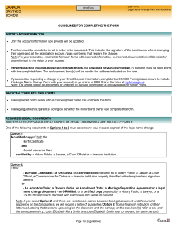


© Copyright 2026