1. No category

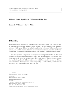
Contents
2 groups
Hideyuki TAKAGI
Kyushu University, Japan
・unpaired ｔ -test
・paired ｔ -test
How to Show Significance?
fitness
fitness
Just compare averages visually?
It is not scientific.
generations
・ two-way ANOVA
one-way
data
・Kruskal-Wallis test
・sign test
・Wilcoxon signed-ranks test
two-way
data
・Friedman test
＋
ver. July 15, 2013
ver. July 11, 2013
ver. April 23, 2013
proposed EC1
・ one-way ANOVA
・Mann-Whitney U-test
http://www.design.kyushu-u.ac.jp/~takagi/
conventional
EC
ANOVA
(Analysis of Variance)
unpaired
unpaired
paired
paired
(related) (independent) (related) (independent)
Slides are at
http://www.design.kyushu-u.ac.jp/~takagi/TAKAGI/StatisticalTests.html
Parametric Test
(normality)
Computational Intelligence Research and
Human Subjective Tests
(n > 2)
data
distribution
Non-parametric Test
(no normality)
Statistical Tests for
n groups
conventional
EC
proposed EC2
Scheffé's method of paired comparison for Human Subjective Tests
How to Show Significance?
Sound design concept: exiting
sound made by
conventional IEC
sound made by
proposed IEC1
sound made by
proposed IEC2
generations
Fig. XX Average convergence curves of n times of trial runs.
Which method is good to make exiting sound?
How to show it?
statistical test
Which Test Should We Use?
2 groups
n groups
・Mann-Whitney U-test
・sign test
・Wilcoxon signed-ranks test
ANOVA
・paired ｔ -test
・ one-way ANOVA
・ two-way ANOVA
one-way
data
・Kruskal-Wallis test
two-way
data
・Friedman test
2 groups
(n > 2)
n groups
(n > 2)
・sign test
・Wilcoxon signed-ranks test
two-way
data
・Friedman test
ANOVA
・unpaired ｔ -test
(Analysis of Variance)
(normality)
paired unpaired
(related) (independent)
unpaired
・Kruskal-Wallis test
n-th generation
(independent)
n-th generation
one-way
data
paired
(related)
・Mann-Whitney U-test
・ two-way ANOVA
(no normality)
・paired ｔ -test
・ one-way ANOVA
Non-parametric Test Parametric Test
・unpaired ｔ -test
ANOVA
data
distribution
(Analysis of Variance)
paired unpaired
(related) (independent)
unpaired
(independent)
paired
(related)
(normality)
(no normality)
(n > 2)
Which Test Should we Use?
data
distribution
Non-parametric Test Parametric Test
・unpaired ｔ -test
(Analysis of Variance)
(normality)
paired unpaired
(related) (independent)
unpaired
(independent)
paired
(related)
My method is
significantly better!
n groups
data
distribution
(no normality)
Papers without statistics tests may be rejected.
2 groups
Non-parametric Test Parametric Test
You cannot show the superiority of
your method without statistical tests.
Which Test Should We Use?
Normality Test
・ one-way ANOVA
• Anderson-Darling test
・ two-way ANOVA
• D'Agostino-Pearson test
• Kolmogorov-Smirnov test
• Shapiro-Wilk test
one-way
・Mann-Whitney
U-test
・Kruskal-Wallis test
• Jarque–Bera
test
data
・・・・
・paired ｔ -test
・sign test
・Wilcoxon signed-ranks test
two-way
data
・Friedman test
Which Test Should We Use?
2 groups
n groups
Which Test Should We Use?
3.75
4.42
3.22
3
one-way
4
data
3.63
・Mann-Whitney U-test
4.08
3.99
5
4.08
3.99
3.65
two-way
6
data
3.98
3.65
3.63
3.75
・sign test
3.98
・Wilcoxon signed-ranks test
・Kruskal-Wallis
test
4.42
3.22
・Friedman test
・sign test
・Wilcoxon signed-ranks test
one-way
data
・Kruskal-Wallis test
two-way
data
・Friedman test
paired unpaired
(related) (independent)
・ two-way ANOVA
unpaired
proposed
(independent)
・Mann-Whitney U-test
GA
paired
(related)
・paired ｔ -test
initial
data #
(normality)
B group data
data
distribution
(no normality)
A group data
paired
data ANOVA
・ one-way
(related)
・paired ｔ -test
・Mann-Whitney U-test
・sign test
・Wilcoxon signed-ranks test
initial
data #
paired
data ANOVA
・ one-way
(related)
GA
proposed
・ two-way ANOVA
one-way
data
・Kruskal-Wallis test
two-way
data
・Friedman test
conditions
2 groups to use statisticalntests
groupsfor (n > 2)
paired data and reduce the # of trial runs?
Non-parametric Test Parametric Test
(independent)
ANOVA
ｔ -test data
・unpairedunpaired
(Analysis of Variance)
paired unpaired
(related) (independent)
unpaired
(independent)
paired
(related)
(normality)
(no normality)
Non-parametric Test Parametric Test
(n > 2)
Which
Test Should We Use?
Q2: How should you design your experimental
Q1: Which tests are more sensitive,
2those
groups
groups data?
(n > 2)
for unpaired data ornpaired
A1: Statistical tests for paired data
because of more data information.
B group data
ANOVA
3.30
A group data
(Analysis of Variance)
3.21
3.3
(independent)
A2: Use the same initialized data for the set of
(method A, method B) at each trial run.
・unpaired ｔ -test
・paired ｔ -test
・Mann-Whitney U-test
・sign test
ANOVA
2
3.21
ANOVA
ｔ -test data
・unpairedunpaired
(Analysis of Variance)
4.23
2.51
・ two-way
paired unpaired
(related) (independent)
1
unpaired
proposed
(independent)
conven
tional
paired
(related)
2.51
initial
data #
(normality)
・paired ｔ 4.23
-test
group B
(no normality)
group A
paired
data ANOVA
・ one-way
(related)
Non-parametric Test Parametric Test
(independent)
ANOVA
ｔ -test data
・unpairedunpaired
Which Test Should We Use?
data
distribution
n groups
data
distribution
(Analysis of Variance)
paired unpaired
(related) (independent)
unpaired
(independent)
paired
(related)
(no normality)
(normality)
data
distribution
Non-parametric Test Parametric Test
2 groups
(n > 2)
・ one-way ANOVA
・ two-way ANOVA
significant?
one-way
data
・Kruskal-Wallis test
two-way
data
・Friedman test
・Wilcoxon signed-ranks
test
n-th generation
t -Test
Which
Test Should we Use?
Q3: Which statistical tests are sensitive,
parametric
tests or non-parametric
2 groups
n groups ones
(n > 2)
and why?
・sign test
・Wilcoxon signed-ranks test
two-way
data
・Friedman test
ANOVA
・unpaired ｔ -test
ｔ -test
・paired ｔ -test
・Mann-Whitney U-test
・sign test
・Wilcoxon signed-ranks test
(Analysis of Variance)
(normality)
paired unpaired
(related) (independent)
unpaired
・Kruskal-Wallis test
(independent)
one-way
data
paired
(related)
・Mann-Whitney U-test
・ two-way ANOVA
(no normality)
・paired ｔ -test
・ one-way ANOVA
n groups
(n > 2)
data
distribution
Non-parametric Test Parametric Test
・unpaired ｔ -test
ANOVA
A3: Parametric tests which can use information
of assumed data distribution.
(Analysis of Variance)
paired unpaired
(related) (independent)
unpaired
(independent)
paired
(related)
(normality)
(no normality)
Non-parametric Test Parametric Test
data
distribution
2 groups
・ one-way ANOVA
・ two-way ANOVA
one-way
data
・Kruskal-Wallis test
two-way
data
・Friedman test
t-Test
t-Test
How to Show Significance?
g
Test this difference with assuming no difference.
（null hypothesis）
significant?
n-th generation
A
B
12
10
14
9
14
7
11
15
16
11
19
10
significant
difference?
Conditions to use t-tests:
(1) normality
(2) equal variances
t-Test
t-Test
Excel (32 bits version only?) has t-tests and ANOVA in Data Analysis
Tools. You must install its add-in. (File -> option -> add-in, and set its add-in.)
F-Test
Test this difference with assuming no difference.
（null hypothesis）
Normality Test
A
12
14
14
11
B
10 (p > 0.05), we assume
When
that
9 there is no significant
difference between σ2A and σ2B .
7
15
16
11
19
10
• Anderson-Darling test
significant
• D'Agostino-Pearson test
difference?
• Kolmogorov-Smirnov test
• Shapiro-Wilk test
• Jarque–Bera test
・・・・
Conditions to use t-tests:
(1) normality
(2) equal variances
t-Test
t-Test
(1) t-Test: Pairs two sample for means
significant?
This is a case when each pair of two
methods with the same initial condition.
n-th generation
(2) t-Test: Two-sample assuming
equal variances
(3) t-Test: Two-sample assuming
unequal variances: Welch's t-test
sample data
A
B
4.23
2.51
3.21
3.31
3.63
3.75
4.42
3.22
4.08
3.99
3.98
3.65
3.68
3.35
4.18
3.93
3.85
3.91
3.71
3.82
t-Test: Paired Two Sample for Means
Mean
Variance
Observations
Pearson Correlation
Hypothesized Mean
Difference
df
t Stat
P(T<=t) one-tail
t Critical one-tail
P(T<=t) two-tail
t Critical two-tail
Variable 1
Variable 2
3.897
3.544
0.125823333 0.208693333
10
10
-0.161190073
0
9
1.794964241
0.053116886
1.833112933
0.106233772
2.262157163
t-Test
t-Test
sample data
t-Test:
Paired
Two
for Means
When p-value is less
than 0.01
or 0.05,
weSample
assume that
there is significant difference with the level
of significance
Variable
1
Variable 2
A
B
of (p < 0.01) or (p < 0.05).
Mean
3.897
3.544
4.23
2.51
Variance
0.125823333 0.208693333
3.21
3.31
Observations
10
10
3.63
3.75
2.5%
Pearson
-0.161190073 5%
2.5%Correlation
4.42
3.22
Mean When A>B never happens,
A ≈ BHypothesized
A<B
A
>B
0
Difference
4.08
3.99
you may use a one-tail test.
df
9
3.98
3.65
t Stat
1.794964241
3.68
3.35
P(T<=t) one-tail
0.053116886
4.18
3.93
t Critical one-tail
1.833112933
3.85
3.91
P(T<=t) two-tail
0.106233772
3.71
3.82
t Critical two-tail
2.262157163
n groups
Difference between two groups
is significant (p < 0.01).
・sign test
・Wilcoxon signed-ranks test
ANOVA
(Analysis of Variance)
paired unpaired
(related) (independent)
unpaired
(independent)
paired
(related)
(normality)
(no normality)
Non-parametric Test Parametric Test
・Mann-Whitney U-test
significant?
・paired ｔ -test
We cannot say that there is
a significant difference
between two group.
(n > 2)
data
distribution
・unpaired ｔ -test
(2) t-Test: Two-sample assuming
equal variances
ANOVA: Analysis of Variance
ANOVA: Analysis of Variance
2 groups
(1) t-Test: Pairs two sample for means
・ one-way ANOVA
ANOVA
・ two-way ANOVA
one-way
data
・Kruskal-Wallis test
two-way
data
・Friedman test
n-th generation
ANOVA: Analysis of Variance
ANOVA: Analysis of Variance
1. Analysis of more than two data groups.
2. Normality and equal variance are required.
1. Analysis of more than two data groups.
2. Normality and equal variance are required.
Excel has ANOVA in
Data Analysis Tools.
Excel has ANOVA in
Data Analysis
.
Check Tools
it using
A
B
A
B
11.0
12.8
C
9.4
11.0
12.8
9.4
9.3
11.3
12.4
9.3
11.3
12.4
11.5
9.5
16.8
16.4
14.0
14.3
16.0
15.2
15.0
13.0
12.8
C
A
B
C
11.5
9.5
16.8
16.4
14.0
14.3
17.0
16.0
15.2
17.0
14.6
15.0
13.0
14.6
12.4
17.0
12.8
12.4
17.0
13.6
15.0
14.3
13.6
15.0
14.3
13.0
12.4
15.6
13.0
12.4
15.6
12.0
17.8
15.0
12.0
17.8
15.0
13.4
12.6
18.6
13.4
12.6
18.6
10.0
13.4
12.4
10.0
13.4
12.4
10.8
16.8
15.4
10.8
16.8
15.4
ANOVA: Analysis of Variance
the Bartlett test.
C
A
three t-tests
B
= one ANOVA
Three times of t-test with (p<0.05) equivalent
one ANOVA (p<0.14).
1-(1-0.05)3 = 0.14
ANOVA: Analysis of Variance
Q1: What are "single factor" and "two factors"?
A1: A column factor (e.g. three groups) and
a sample factor (e.g. initialized condition).
n-th generation
When data correspond each other, use
two-way ANOVA (two-factor ANOVA).
When data are independent, use
one-way ANOVA
column(single
factor factor ANOVA).
When data correspond each other, use
two-way ANOVA
(two-factor
column
factor ANOVA).
sample factor
When data are independent, use
one-way ANOVA (single factor ANOVA).
ANOVA: Analysis of Variance
ANOVA: Analysis of Variance
two-factor (two-way) ANOVA
Source of Variation
Between Groups
Within Groups
We cannot say that three groups
are significantly different. (p=0.089)
initial
group A group B group C
condition
#1
4.23
2.51
3.04
#2
3.21
3.3
2.89
#3
3.63
3.75
3.55
#4
4.42
3.22
4.39
#5
4.08
3.99
3.86
#6
3.98
3.65
3.5
#7
3.75
2.62
3.6
#8
3.22
2.93
3.21
Total
11.50523
Source of Variation
Sample
Columns
Interaction
Within
Total
2
1
2
12
MS
F
P-value
F crit
0.377617 2.755097 0.103596 3.885294
3.582272 26.13631 0.000256 4.747225
0.069706 0.508573 0.613752 3.885294
0.137061
17
A
B
C
11.0
12.8
9.4
9.3
11.3
12.4
11.5
9.5
16.8
16.4
14.0
14.3
16.0
15.2
17.0
15.0
13.0
14.6
12.8
12.4
17.0
13.6
15.0
14.3
13.0
12.4
15.6
12.0
17.8
15.0
13.4
12.6
18.6
10.0
13.4
12.4
10.8
16.8
15.4
n groups
(n > 2)
11.3
12.4
11.5
9.5
16.8
16.4
14.0
14.3
16.0
15.2
17.0
15.0
13.0
14.6
12.8
12.4
17.0
13.6
15.0
14.3
13.0
12.4
15.6
12.0
17.8
15.0
13.4
12.6
18.6
10.0
13.4
12.4
10.8
16.8
15.4
paired unpaired
(related) (independent)
9.4
9.3
unpaired
C
(independent)
B
12.8
(normality)
A
11.0
・unpaired ｔ -test
・ one-way ANOVA
If normality and equal variances are not
guaranteed, use non-parametric tests.
paired
(related)
significant?
Column
factor
(no normality)
17
Column
factor
data
distribution
Non-parametric Test Parametric Test
6.12165
df
2 groups
Sample factor
Total
MS
F
P-value
F crit
0.377617 2.755097 0.103596 3.885294
3.582272 26.13631 0.000256 4.747225
0.069706 0.508573 0.613752 3.885294
0.137061
When (p-value < 0.01 or 0.05),
there is(are) significant difference
somewhere among data groups.
Non-Parametric Tests
(Fisher's PLSD method, Scheffé method, Bonferroni-Dunn test, Dunnett
method, Williams method, Tukey method, Nemenyi test, Tukey-Kramer
method, Games/Howell method, Duncan's new multiple range test,
Student-Newman-Keuls method, etc. Each has different characteristics.)
2
1
2
12
29
F crit
3.354131
• Significant difference among Sample (e.g. initial
conditions) cannot be found (p > 0.05).
• Significant difference can be found somewhere
among Columns (e.g. three methods) (p < 0.01).
• We need not care an interaction effect between two
factors (e.g. initial condition vs. methods) (p > 0.05).
There are significant difference
somewhere among three groups.
(p<0.05)
A1: Apply multiple comparisons between all pairs
among columns.
df
SS
0.755233
3.582272
0.139411
1.644733
6.12165
Q1: Where is significant among A, B, and C?
SS
0.755233
3.582272
0.139411
1.644733
MS
F
P-value
2 3.05671 15.30677 3.6E-05
27 0.199697
Output of the two-way ANOVA
ANOVA: Analysis of Variance
Source of Variation
Sample
Columns
Interaction
Within
df
ANOVA
group A group B group C
4.23
2.51
3.04
3.21
3.3
2.89
3.63
3.75
3.55
4.42
3.22
4.39
4.08
3.99
3.86
3.98
3.65
3.5
3.75
2.62
3.6
3.22
2.93
3.21
SS
6.11342
5.39181
Sample factor
column factor
sample factor
column factor
Output of the one-way ANOVA
(Analysis of Variance)
one-factor (one-way) ANOVA
・paired ｔ -test
・Mann-Whitney U-test
・sign test
・Wilcoxon signed-ranks test
・ two-way ANOVA
one-way
data
・Kruskal-Wallis test
two-way
data
・Friedman test
Mann-Whitney U-test
Mann-Whitney U-test
2 groups
n groups
(Wilcoxon-Mann-Whitney test, two sample Wilcoxon test)
(n > 2)
1. Comparison of two groups.
2. Data have no normality.
3. There are no data corresponding
between two groups (independent).
ANOVA
・unpaired ｔ -test
・paired ｔ -test
・Mann-Whitney
U-test
・sign test
・Wilcoxon signed-ranks test
(Analysis of Variance)
paired unpaired
(related) (independent)
unpaired
(independent)
paired
(related)
(normality)
(no normality)
Non-parametric Test Parametric Test
data
distribution
?
・ one-way ANOVA
no normality
?
・ two-way ANOVA
one-way
data
・Kruskal-Wallis test
two-way
data
・Friedman test
n-th generation
Mann-Whitney U-test
Mann-Whitney U-test (cont.)
(Wilcoxon-Mann-Whitney test, two sample Wilcoxon test)
(Wilcoxon-Mann-Whitney test, two sample Wilcoxon test)
1. Calculate a U value.
2. See a U-test table.
• Use the smaller value of U or U'.
• When n1 ≤ 20 and n2 ≤ 20 , see a Mann-Whitney test table.
(where n1 and n2 are the # of data of two groups.)
• Otherwise, since U follows the below normal distribution roughly,
0
2
3
4
U =0+2+3+4=9
U' = 11 (U + U' = n1n2)
two values are the same,
)
( when
count as 0.5.
 n n n n (n  n  1) 
N U ,  U2  N  1 2 , 1 2 1 2

12
 2

U  U
normalize U as z 
and check a standard normal distribution table
U
n1n2
n1n2 (n1  n2  1)
with the z, where U 
and  U 
.
2
12


Examples: Mann-Whitney U-test
Exercise: Mann-Whitney U-test
(Wilcoxon-Mann-Whitney test, two sample Wilcoxon test)
(Wilcoxon-Mann-Whitney test, two sample Wilcoxon test)
Ex.1
Ex.2
0
2
3.5
5
2.5
4
5
3
4
U = 9
U' = 11
(p < 0.05)
n2
4
n1
2.5
Ex.3
0
0.5
5
4
5
6
5
U = 12
U' = 13
6
U = 23.5
U' = 1.5
5
6
・・・
n1
n2
4
5
(p < 0.01)
6
・・・
(p < 0.05)
n2
4
n1
6
7
n1
n2
4
5
(p < 0.01)
6
7
・・・
・・・
・・・
・・・
ー
・・・
・・・
・・・
3
ー
0
1
1
3
ー
ー
ー
ー
4
0
1
2
・・・
4
ー
ー
0
・・・
4
0
1
2
3
4
ー
ー
0
0
2
3
・・・
5
1
1
・・・
5
2
3
5
5
1
1
1
・・・
・・・
・・・
・・・
・・・
6
5
6
6
2
3
Sign Test
Sign Test
2 groups
n groups
(n > 2)
（1）Sign Test
significance test between the # of winnings and losses
unpaired
paired
(related)
(independent)
・paired ｔ -test
・Mann-Whitney U-test
・sign test
・Wilcoxon signed-ranks test
ANOVA
・unpaired ｔ -test
(Analysis of Variance)
paired unpaired
(related) (independent)
data
distribution
(normality)
5
U' > 5, (p > 0.05):
(Since
significance is not found )
ー
・・・
(no normality)
U = 29.5
U' = 6.5
6
・・・
5
Non-parametric Test Parametric Test
5
one-way
data
two-way
data
・ one-way ANOVA
・ two-way ANOVA
・Kruskal-Wallis test
・Friedman test
（2）Wilcoxon's Signed Ranks Test
significance test using both the # of winnings and losses
and the level of winnings/losses
data of
2 groups
173
174
143
137
158
151
156
143
176
180
165
162
# of winnings
and losses
+
+
+
+
+
+
-
the level of
winnings/losses
-1
+6
+7
+13
-4
+3
Sign Test
Sign Test
Fig.3 in
1. Calculate the # of winnings and
losses by comparing runs with the
same initial data.
2. Check a sign test table to show
significance of two methods.
n-th generation
Sign Test
Task Example
Whether performances of pattern recognition
methods A and B are significantly different?
n1 cases: Both methods succeeded.
n2 cases: Method A succeeded, and method B failed.
n3 cases: Method A failed, and method B succeeded.
n4 cases: Both methods failed.
How to check?
1.
2.
3.
Set N = n2 + n3.
Check the right table with the N.
If min(n2, n3) is smaller than the number for the N,
we can say that there is significant difference with
the significant risk level of XX.
Exercise
Whether there is significant difference for
n2 = 12 and n3 = 28?
ANSWER:
Check the right table with N = 40.
As n2 is bigger than 11 and smaller than 13, we can say
that there is a significant difference between two with
(p < 0.05) but cannot say so with (p < 0.01).
Y. Pei and H. Takagi, "Fourier analysis of the fitness
landscape for evolutionary search acceleration," IEEE
Congress on Evolutionary Computation (CEC), pp.1-7,
Brisbane, Australia (June 10-15, 2012).
The (+,-) marks show whether our proposed
methods converge significantly better or poorer
than normal DE, respectively, (p ≤0.05).
Fig.2 in the same paper.
level of
significance
%
%
level of
significance
%
%
F1: DE_N vs. DE_LR
F1: DE_N vs. DE_LS
F1: DE_N vs. DE_FR_GLB_nD
F1: DE_N vs. DE_FR_LOC_nD
F1: DE_N vs. DE_FR_GLB_1D
F1: DE_N vs. DE_FR_LOC_1D
F2: DE_N vs. DE_LR
F2: DE_N vs. DE_LS
F2: DE_N vs. DE_FR_GLB_nD
F2: DE_N vs. DE_FR_LOC_nD
F2: DE_N vs. DE_FR_GLB_1D
F2: DE_N vs. DE_FR_LOC_1D
F3: DE_N vs. DE_LR
F3: DE_N vs. DE_LS
F3: DE_N vs. DE_FR_GLB_nD
F3: DE_N vs. DE_FR_LOC_nD
F3: DE_N vs. DE_FR_GLB_1D
F3: DE_N vs. DE_FR_LOC_1D
F4: DE_N vs. DE_LR
F4: DE_N vs. DE_LS
F4: DE_N vs. DE_FR_GLB_nD
F4: DE_N vs. DE_FR_LOC_nD
F4: DE_N vs. DE_FR_GLB_1D
F4: DE_N vs. DE_FR_LOC_1D
F5: DE_N vs. DE_LR
F5: DE_N vs. DE_LS
F5: DE_N vs. DE_FR_GLB_nD
F5: DE_N vs. DE_FR_LOC_nD
F5: DE_N vs. DE_FR_GLB_1D
F5: DE_N vs. DE_FR_LOC_1D
F6: DE_N vs. DE_LR
F6: DE_N vs. DE_LS
F6: DE_N vs. DE_FR_GLB_nD
F6: DE_N vs. DE_FR_LOC_nD
F6: DE_N vs. DE_FR_GLB_1D
F6: DE_N vs. DE_FR_LOC_1D
F7: DE_N vs. DE_LR
F7: DE_N vs. DE_LS
F7: DE_N vs. DE_FR_GLB_nD
F7: DE_N vs. DE_FR_LOC_nD
F7: DE_N vs. DE_FR_GLB_1D
F7: DE_N vs. DE_FR_LOC_1D
F8: DE_N vs. DE_LR
F8: DE_N vs. DE_LS
F8: DE_N vs. DE_FR_GLB_nD
F8: DE_N vs. DE_FR_LOC_nD
F8: DE_N vs. DE_FR_GLB_1D
F8: DE_N vs. DE_FR_LOC_1D
Generations
0
10
20
30
40
50
|__________|__________|__________|__________|__________|
+++++++++++++++++++++++++++++++++++++++++++++++++
+++++++++++++++++++++++++++++++++++++++++++++++++
+ +++++++++++++++++++++++++++++++++++++
++ ++++++++++++++++++++++++++++++++++++
+ +++++++++++++++++++++++++++++++++++++
+++ ++++++++++++++++++++++++++++++++++++
+ ++++++++++++++++++++++++++++++++++++++++++
++++++++++++++++++++++++++++++++++++++++++++
++++++++++++++++++++++++
++
+++++++++++++++++++++++++++++++++++++++++++++++++
++++++++++++++++++++++++++++++++++++++++++++++++++
++++++++++++++++++++++++++++++++++++++++++++++
+ ++++++++++++++++++++++++++++++++++++++++++++++
++++++++++++++++++++++++++++++++++++++++++++++
+ ++ +
+++++++++++++++++++
++
+++
+
++++++++++++ +
+++++++
+++++++++++++++++++++++++++++++++++ +++++
+ + +++++++++++++++++++++++++++++++++++
+++++++++++++++++++++++++++++++++
+ + +++++++++++++++++++++++++++++++++++
+++++++++ ++++++++++++++++++++++ +++
+
+
+
++++++ + ++
+++++++++++++++++++++++++++++++++++
++++++++++++++++++++++++++++++++++++++++++++++++
+++++++++++++++++++++++++++++++++++++++++++++++
+
+++++++++++++++++++++++++++++++++++
+++ +++++++++++++++++++++++++++++++++++++++++++++
Sign Test
Let's think about the case of N = 17.
To say that n1 and n2 are significantly different,
(n1 vs. n2) = (17 vs. 0), (16 vs. 1), or (15 vs. 2) (p < 0.01)
or
(p < 0.05)
(n1 vs. n2) = (14 vs. 3) or (13 vs. 4)
level of significance
%
%
Exercise: Sign Test
Wilcoxon Signed-Ranks Test
level of significance
%
%
2 groups
Wilcoxon Signed-Ranks Test
Q: When a sign test could not show significance,
how to do?
A: Try the Wilcoxon signed-ranks test. It is more sensitive
than a simple sign test due to more information use.
・paired ｔ -test
・Mann-Whitney U-test
・sign test
・Wilcoxon signed-ranks test
・ one-way ANOVA
・ two-way ANOVA
one-way
data
・Kruskal-Wallis test
two-way
data
・Friedman test
Wilcoxon Signed-Ranks Test
（1）Sign Test
significance test between the # of winnings and losses
（2）Wilcoxon's Signed Ranks Test
significance test using both the # of winnings and losses
and the level of winnings/losses
data of
2 groups
n-th generation
ANOVA
・unpaired ｔ -test
(Analysis of Variance)
paired unpaired
(related) (independent)
unpaired
(independent)
18 vs. 5
paired
(related)
9 vs. 3
(normality)
14 vs. 1
(no normality)
16 vs. 4
(n > 2)
data
distribution
Non-parametric Test Parametric Test
Check the significance of:
n groups
173
174
143
137
158
151
156
143
176
180
165
162
# of winnings
and losses
+
+
+
+
+
+
-
the level of
winnings/losses
-1
+6
+7
+13
-4
+3
Wilcoxon Signed-Ranks Test
182
169
172
143
158
156
176
165
n=8
T=3
T=3 ≤ 3 (n=8, p<0.05),
then difference between systems A and B is significant.
Example:
v (system A)
(step 1)
v (system B) difference d
163
142
173
137
151
143
172
168
(step 2)
(step 3)
add sign to
the ranks
7
8
－1
4
5
6
3
－2
rank of |d|
19
27
－1
6
7
13
4
－3
7
8
1
4
5
6
3
2
n8
(step 4)
rank of fewer
# of signs
T=3 > 0 (n=8, p<0.01),
then we cannot say there is a significant difference.
1
When n > 25
As T follows the below normal distribution roughly,
2
(step 5) T   # of ( Step 4)
3
(step 6)
 n(n  1) n(n  1)(2n  1) 
,
N T ,  T2  N 

24
 4


z
Wilcoxon Signed-Ranks Test
(step 1)
176
142
172
143
158
156
176
165
(step 2)
(step 3)
add sign to
v (system B) difference d rank of |d|
the ranks
163
13
7 → 6.5 Tip #2 6.5
142
0 Tip #1
173
1
－1
－1
137
6
4
4
151
7
5
5
143
13
6 → 6.5 Tip #2 6.5
172
4
3
3
168
2
－3
－2
1
2
9
1
4
2
5
7 8
T  T
T
(step 1)
v (system A) v (system B)
182
163
169
142
173
172
143
137
158
151
156
143
176
172
165
168
difference d
(step 2)
rank of |d|
n=
(step 6)
Wilcoxon test table
3
6
one-tail
p < 0.025
p < 0.005
two-tail
p < 0.05
p < 0.01
0
2
3
5
8
10
13
17
21
25
29
34
40
46
52
58
65
73
81
89
0
1
3
5
7
9
12
15
19
23
27
32
37
42
48
54
61
68
n= 6
7
8
9
10
11
12
13
14
15
16
17
18
19
20
21
22
23
24
25
Exercise 1: Wilcoxon Signed-Ranks Test
(step 4)
rank of fewer
# of signs
Give the average rank
6.5 = (5+6+7+8)/4. 10
Tips:
1. When d = 0, ignore the data.
2. When there are the same ranks of |d|,
give average ranks.

normalize T as the below and check a standard
normal distribution table with the z; see T and  T
in the above equation.
Wilcoxon test table
v (system A)
Wilcoxon Test Table:
significance point of T
(step 6)
(step 3)
add sign to
the ranks
(step 4)
rank of fewer
# of signs
(step 5) T   # of ( Step 4)
T=
Exercise 1: Wilcoxon Signed-Ranks Test
(step 1)
v (system A) v (system B)
(step 2)
difference d
rank of |d|
(step 3)
add sign to
the ranks
7
(step 4)
rank of fewer
# of signs
Exercise 2: Wilcoxon Signed-Ranks Test
(step 1)
v (system A) v (system B)
182
163
19
7
27
31
169
142
27
8
8
20
25
173
172
1
1
1
34
33
143
137
6
4
4
25
27
5
31
31
6
23
29
26
27
24
30
35
34
158
151
7
5
156
143
13
6
3
-2
176
172
4
3
165
168
-3
2
2
(step 5) T   # of ( Step 4)
T=2
n=8
(step 6)
Wilcoxon test table
As T(=2) < 3, there is a significant difference between A and B (p<0.05).
But, as 0 < T(=2), we cannot say so with the significance level of (p<0.01).
Exercise 2: Wilcoxon Signed-Ranks Test
(step 1)
27
31
-4
5
(step 3)
add sign to
the ranks
-5
20
25
-5
6
-6
34
33
1
2
2
4
-4
v (system A) v (system B)
(step 2)
difference d
rank of |d|
25
27
-2
31
31
0
23
29
-6
7.5
-7.5
26
27
-1
2
-2
24
30
-6
7.5
-7.5
35
34
1
2
2
difference d
(step 6)
Wilcoxon test table
As T > 3, we cannot say that there is a
significant difference between A and B.
rank of |d|
(step 3)
add sign to
the ranks
(step 6)
Wilcoxon test table
Exercise 3: Wilcoxon Signed-Ranks Test
(step 4)
rank of fewer
# of signs
2
(step 4)
rank of fewer
# of signs
(step 5) T   # of ( Step 4)
n=
Explain how to apply this test to test
whether two groups are significantly
different at the below generation?
(No need to care the case of d = 0.)
n = 8 (no count for d = 0.)
(step 2)
2
(step 5) T   # of ( Step 4)
T=4
n-th generation
2 groups
n groups
(n > 2)
1. Comparison of more than two groups.
2. Data have no normality.
3. There are no data corresponding
among groups (independent).
ANOVA
・unpaired ｔ -test
・paired ｔ -test
・Mann-Whitney U-test
・sign test
・Wilcoxon signed-ranks test
(Analysis of Variance)
paired unpaired
(related) (independent)
unpaired
(independent)
paired
(related)
(normality)
(no normality)
Non-parametric Test Parametric Test
data
distribution
・ one-way ANOVA
・ two-way ANOVA
?
?
?
no normality
Kruskal-Wallis Test
Kruskal-Wallis Test
・Kruskal-Wallis test
two-way
data
・Friedman test
n-th generation
Kruskal-Wallis Test
Kruskal-Wallis Test
Let's use ranks of data.
1
2
4
6
8
11
14
13
15
16
N: total # of data
k: # of groups
ni: # of data of group i
Ri : sum of ranks of group i
3
1
5
2
7
4
9
10
12
6
3
5
7
8
11
14
13
15
16
9
10
12
17
17
R1 = 38
R2 = 69
R3 = 46
How to Test
1. Rank all data.
2. Calculate N, k, and Ri .
3. Calculate statistical value H.
k
Ri2
12
H
 3( N  1)

N ( N  1) i 1 ni
4. If k = 3 and N ≤ 17, compare
the H with a significant point
in a Kruskal-Wallis test table.
Otherwise, assume that H
follows the χ2 distribution and
test the H using a χ2
distribution table of (k-1)
degrees of freedom
Kruskal-Wallis Test Table
Example: Kruskal-Wallis Test
N = n1+n2+n3
k
(n1, n2, n3)
(R1, R2, R3)
H
n1
2
2
2
2
2
2
2
2
2
2
2
2
2
2
2
2
2
2
2
2
2
2
2
2
2
2
2
2
2
2
2
2
2
2
2
2
2
2
2
2
2
2
= 17 data
= 3 groups
= (6, 5, 6)
= (38, 69, 46)
k
2
i
R
12
  3( N  1)
N ( N  1) i 1 ni

12
 38 * 38 69 * 69 46 * 46 



  3(17  1)
17(17  1)  6
5
6 
= 6.609
Since significant points of (p<0.05) and (p<0.01)
for (n1, n2, n3) = (6, 5, 6) are 5.765 and 8.124,
respectively, there are significant difference(s)
somewhere among three groups (p<0.05).
5.765
6.609
significance
point of
(p<0.05)
(for k = 3 and N ≤17)
8.124
significance
point of
(p<0.01)
n2
2
2
2
2
2
2
2
2
2
2
2
2
3
3
3
3
3
3
3
3
3
3
4
4
4
4
4
4
4
4
5
5
5
5
5
5
6
6
6
6
7
7
n3 p < 0.05 p < 0.01
2
4.714
3
5.333
4
5.160
6.533
5
5.346
6.655
6
5.143
7.000
7
5.356
6.664
8
5.260
6.897
9
5.120
6.537
10
5.164
6.766
11
5.173
6.761
12
5.199
6.792
13
5.361
3
5.444
6.444
4
5.251
6.909
5
5.349
6.970
6
5.357
6.839
7
5.316
7.022
8
5.340
7.006
9
5.362
7.042
10
5.374
7.094
11
5.350
7.134
12
5.455
7.036
4
5.273
7.205
5
5.340
7.340
6
5.376
7.321
7
5.393
7.350
8
5.400
7.364
9
5.345
7.357
10
5.365
7.396
11
5.339
7.339
5
5.339
7.376
6
5.393
7.450
7
5.415
7.440
8
5.396
7.447
9
5.420
7.514
10
5.410
7.467
6
5.357
7.491
7
5.404
7.522
8
5.392
7.566
9
5.398
7.491
7
5.403
7.571
8
n1
3
3
3
3
3
3
3
3
3
3
3
3
3
3
3
3
3
3
3
3
3
3
3
3
3
4
4
4
4
4
4
4
4
4
4
4
4
5
5
5
5
n2
3
3
3
3
3
3
3
3
3
4
4
4
4
4
4
4
5
5
5
5
5
6
6
6
7
4
4
4
4
4
4
5
5
5
5
6
6
5
5
5
6
n3 p < 0.05 p < 0.01
5.606
7.200
3
5.791
6.746
4
6.649
7.079
5
5.615
7.410
6
5.620
7.228
7
5.617
7.350
8
5.589
7.422
9
5.588
7.372
10
5.583
7.418
11
5.599
7.144
4
5.656
7.445
5
5.610
7.500
6
5.623
7.550
7
5.623
7.585
8
5.652
7.614
9
5.661
7.617
10
5.706
7.578
5
5.602
7.591
6
5.607
7.697
7
5.614
7.706
8
5.670
7.733
9
5.625
7.725
6
5.689
7.756
7
5.678
7.796
8
5.688
7.810
7
5.692
7.654
4
5.657
7.760
5
6.681
7.795
6
5.650
7.814
7
5.779
7.853
8
5.704
7.910
9
5.666
7.823
5
5.661
7.936
6
5.733
7.931
7
5.718
7.992
8
5.724
8.000
6
5.706
8.039
7
5.780
8.000
5
5.729
8.028
6
5.708
8.108
7
5.765
8.124
6
Kruskal-Wallis Test Table
Example: Kruskal-Wallis Test
N = n1+n2+n3
k
(n1, n2, n3)
(R1, R2, R3)
= 17 data
= 3 groups
= (6, 5, 6)
= (38, 69, 46)
(for k = 3 and N ≤17)
n1
2
2
2
2
2
2
2
2
2
2
2
2
2
2
2
2
2
2
2
2
2
2
2
2
2
2
2
2
2
2
2
2
2
2
2
2
2
2
2
2
2
2
n2
2
2
2
2
2
2
2
2
2
2
2
2
3
3
3
3
3
3
3
3
3
3
4
4
4
4
4
4
4
4
5
5
5
5
5
5
6
6
6
6
7
7
n3 p < 0.05 p < 0.01
2
4.714
3
5.333
4
5.160
6.533
5
5.346
6.655
6
5.143
7.000
7
5.356
6.664
8
5.260
6.897
9
5.120
6.537
10
5.164
6.766
11
5.173
6.761
12
5.199
6.792
13
5.361
3
5.444
6.444
4
5.251
6.909
5
5.349
6.970
6
5.357
6.839
7
5.316
7.022
8
5.340
7.006
9
5.362
7.042
10
5.374
7.094
11
5.350
7.134
12
5.455
7.036
4
5.273
7.205
5
5.340
7.340
6
5.376
7.321
7
5.393
7.350
8
5.400
7.364
9
5.345
7.357
10
5.365
7.396
11
5.339
7.339
5
5.339
7.376
6
5.393
7.450
7
5.415
7.440
8
5.396
7.447
9
5.420
7.514
10
5.410
7.467
6
5.357
7.491
7
5.404
7.522
8
5.392
7.566
9
5.398
7.491
7
5.403
7.571
8
Q1: Where is significant among A, B, and C?
k
Ri2
12
multiple
between all pairs
H A1: Apply
 3( Ncomparisons
 1)
N (among
N  1) i 1columns.
ni
(Fisher's PLSD
method, Scheffé method, Bonferroni-Dunn test, Dunnett
3
Ri2 method,
12 Williams
38 * 38 Tukey
69 * 69method,
46 * 46Nemenyi

method,



17 test,
1) Tukey-Kramer

  3(multiple

method,
range test,
17(17 Games/Howell
1) i 1 ni  6 method,
5 Duncan's
6 new

Student-Newman-Keuls method, etc. Each has different characteristics.)
= 6.609
Since significant points of (p<0.05) and (p<0.01)
for (n1, n2, n3) = (6, 5, 6) are 5.765 and 8.124,
respectively, there are significant difference(s)
somewhere among three groups (p<0.05).
5.765
6.609
significance
point of
(p<0.05)
8.124
significance
point of
(p<0.01)
2 groups
11
12
13
There is/are significant difference(s)
somewhere among three groups (p<0.05).
R1 = 24
R2 =
44
R3 =
23
6.227
significance
point of
(p<0.05)
7.760
significance
point of
(p<0.01)
・unpaired ｔ -test
・paired ｔ -test
・Mann-Whitney U-test
・sign test
・Wilcoxon signed-ranks test
ANOVA
= 6.227
5.657
n groups
(Analysis of Variance)
10
9
paired unpaired
(related) (independent)
8
unpaired
7
k
Ri2
12
  3( N  1)
N ( N  1) i 1 ni
(independent)
6
H
paired
(related)
5
(normality)
3
4
n3 p < 0.05 p < 0.01
5.606
7.200
3
5.791
6.746
4
6.649
7.079
5
5.615
7.410
6
5.620
7.228
7
5.617
7.350
8
5.589
7.422
9
5.588
7.372
10
5.583
7.418
11
5.599
7.144
4
5.656
7.445
5
5.610
7.500
6
5.623
7.550
7
5.623
7.585
8
5.652
7.614
9
5.661
7.617
10
5.706
7.578
5
5.602
7.591
6
5.607
7.697
7
5.614
7.706
8
5.670
7.733
9
5.625
7.725
6
5.689
7.756
7
5.678
7.796
8
5.688
7.810
7
5.692
7.654
4
5.657
7.760
5
6.681
7.795
6
5.650
7.814
7
5.779
7.853
8
5.704
7.910
9
5.666
7.823
5
5.661
7.936
6
5.733
7.931
7
5.718
7.992
8
5.724
8.000
6
5.706
8.039
7
5.780
8.000
5
5.729
8.028
6
5.708
8.108
7
5.765
8.124
6
(n > 2)
data
distribution
(no normality)
2
= 13 samples
= 3 groups
= ( 5, 4, 4)
= (24, 44, 23)
Non-parametric Test Parametric Test
1
n2
3
3
3
3
3
3
3
3
3
4
4
4
4
4
4
4
5
5
5
5
5
6
6
6
7
4
4
4
4
4
4
5
5
5
5
6
6
5
5
5
6
Friedman Test
Exercise: Kruskal-Wallis Test
N = n1+n2+n3
k
(n1, n2, n3)
(R1, R2, R3)
n1
3
3
3
3
3
3
3
3
3
3
3
3
3
3
3
3
3
3
3
3
3
3
3
3
3
4
4
4
4
4
4
4
4
4
4
4
4
5
5
5
5
・ one-way ANOVA
・ two-way ANOVA
one-way
data
・Kruskal-Wallis test
・Friedman test
Friedman Test
Friedman Test
When
(1) more than two groups,
(2) data have correspondence (not independent), but
(3) the conditions of two-way ANOVA are not satisfied,
Let' use ranks of data and Friedman test.
methods
benchmark
tasks
a
b
methods
b
c
a
d
A
0.92
0.75
0.65
0.81
B
0.48
0.45
0.41
0.52
C
0.56
0.41
0.47
0.50
D
0.61
0.50
0.56
0.54
4
4
k
12
 
 Ri2  3n(k  1)
nk (k  1) i 1
3
3
d
3
4
3
2
12
# of methods (k = 4)
Step 3: Calculate the Friedman test value,
χ2r
.
k
12
Ri2  3n(k  1)

nk (k  1) i 1
12

152  6 2  7 2  12 2   3 * 4 * 5
4* 4*5
 8.1

8.1
significance
point of
(p<0.05)
9.6
significance
point of
(p<0.01)
method
b
c
2
1
2
1
1
2
1
3
6
7
a
4
3
4
4
15
d
Q1: Where is significant among
a, b, c, or d?
3
Friedman test table.
k
3
Step 4: Since significant point for (k,n) = (4,4) is7.80,
there is/are significant difference(s) somewhere
among four methods, a, b, c, and d (p<0.05).
7.8
.
Example: Friedman Test
benchmark
tasks
A
B
C
D
Σ
4
n
p<0.05 p<0.01
3
6.00
－
4
5
6.50
6.40
8.00
8.40
6
7.00
9.00
7
8
9
∞
3
7.14
6.25
6.22
5.99
7.40
8.86
9.00
9.56
9.21
9.00
4
7.80
9.60
5
7.80
7.81
9.96
11.34
∞
4
3
2
12
A1: Apply multiple comparisons between all pairs
among columns.
Friedman test table.
(Fisher's PLSD method, Scheffé method, Bonferroni-Dunn test, Dunnett
# of methods
(k = 4) Nemenyi test, Tukey-Kramer
method, Williams method,
Tukey method,
k
n
p<0.05 p<0.01
2
method,
Games/Howell
method,
Duncan's
new
multiple
range
test,
Step 3: Calculate the Friedman test value, χ r .
k method, etc. Each has different characteristics.)
Student-Newman-Keuls
3
6.00
－
12
 Ri2  3n(k  1)
nk (k  1) i 1
12

152  6 2  7 2  12 2   3 * 4 * 5
4* 4*5
 8.1
 r2 


3
Step 4: Since significant point for (k,n) = (4,4) is7.80,
there is/are significant difference(s) somewhere
among four methods, a, b, c, and d (p<0.05).
7.8
8.1
significance
point of
(p<0.05)
9.6
significance
point of
(p<0.01)
2
4
3
ranking among methods
χ2r
Step 1: Make a ranking table.
Step 2: Sum ranks of the factor that you want to test.
 r2 

3
1
2
2
1 1
1
1
# of data (n = 4)
method
b
c
2
1
2
1
1
2
1
3
6
7
4
4
3
3
1
Step 4: If k =3 or 4, compare χ2r with a significant point
in a Friedman test table.
Otherwise, use a χ2 table of (k-1) degrees of freedom.
2
4
3
Step 1: Make a ranking table.
Step 2: Sum ranks of the factor that you want to test.
a
4
3
4
4
15
2
where (k, n) are the # of levels of factors 1 and 2.
Example: Friedman Test
benchmark
tasks
A
B
C
D
Σ
methods
b c d
2
r
1
1
2 2
d
3
4
3
2
12
Step 3: Calculate the Friedman test value,
3
2
a
4
3
4
4
15
4
# of methods (k = 4)
d
4
c
method
b
c
2
1
2
1
1
2
1
3
6
7
# of data
(n = 4)
benchmark
tasks
A
B
C
D
Σ
a
# of data (n = 4)
(ex.) Comparison of recognition rates.
Step 1: Make a ranking table.
Step 2: Sum ranks of the factor that you want to test.
4
4
5
6.50
6.40
8.00
8.40
6
7.00
9.00
7
8
9
∞
3
7.14
6.25
6.22
5.99
7.40
8.86
9.00
9.56
9.21
9.00
4
7.80
9.60
5
7.80
7.81
9.96
11.34
∞
2 groups
n groups
(n > 2)
data
distribution
room lighting design by
optimizing LED assignments
lighting design
of 3-D CG
Corridor
normality
(parametric)
ｔ -test
Target
System
W
ANOVA
one-way ANOVA
(Analysis of
Variance)
two-way ANOVA
K
Wall
(non-parametric)
・sign test
one-way
data
・kruskal-wallis test
・Wilcoxon Signed-Ranks Test
two-way
data
・Friedman test
Verenda
C an
yo u
hear
me ?
Interactive Evolutionary Computation
room layout
planning design
hearing-aid fitting
measuring
mental scale
geological simulation
MEMS design
Scheffé's Method of Paired Comparison
Scheffé's Method of Paired Comparison
ANOVA based on nC2 paired comparisons for n objects.
Original method and three modified methods
All subjects must evaluate all pairs.
better
slightly
better even
slightly
better even
slightly
better better
no
ANOVA
order effect
better
slightly
better better
yes
no
slightly
better better
significance check
using a yardstick
(1)
and then
(2)
and then
may result different evaluation.
yes
original
Ura's variation
(原法, 1952)
（浦の変法, 1956)
Haga's variation
Order Effect
slightly
better better even
??
IEC
＋
Scheffé's method of paired comparison for Human Subjective Tests
subjective
evaluations
Evolutionary
Computation
L
B
no normality
image enhancement processing
Scheffé's Method of Paired Comparison
Scheffé's Method of Paired Comparison
（芳賀の変法）
Nakaya's variation
（中屋の変法, 1970)
Scheffé's Method of Paired Comparison
1. Ask N human subjects to evaluate t objects in 3, 5 or 7 grades.
2. Assign [-1, +1], [-2, +2] or [-3, +3] for these grades.
3. Then, start calculation (see other material).
better
better
slightly
slightly
better even better better
slightly
slightly
better even better better
What is the best present to be her/his boy/girl friend?
[SITUATION] He/he is my longing. I want to be her/his boy/girl friend
before we graduate from our university. To get over my one-way love, I
decided to present something of about 3,000 JPY and express my heart.
I show you 5C2 pairs of presents. Please compare each pair and mark
your relative evaluation in five levels.
Total row data
Paired comparisons
for t=3 objects.
Questionnaire
Application Example:
O1
O2
O3
O4
O5
O6
A1 - A2
2
1
1
2
1
2
A1 - A3
2
2
1
1
1
1
A2 - A3
1
0
1
1
-1
0
・・・
slightly
slightly
better better even better better
strap for
a mobile phone
invitation to
a dinner
tea /coffee
stuffed animal fountain pen

Ex. Q.
・・・・
Six subjects (N = 6)

Results of Scheffé's Method of Paired Comparison (Nakaya's variation)
Scheffé's Method of Paired Comparison
What is the best present to be her/his boy/girl friend?
Modified methods byy Ura and Nakaya
y
(significant difference)
present from a female
Original method and three modified methods
How about tea leave
or a stuffed anima?
I will catch her
heart by dinner.
All subjects must evaluate all pairs.
0.5
1
-1
more
effective
-0.5
I hesitate to accept it
as we have not gone
about with him.
-0.5
0
0.5
1
0.5
1
Eat! Eat! Eat!
more
effective
less
effective
-1
0
-1
-0.5
0
0.5
1
order effect
0
more
effective
-0.5
less
effective
-1
more
effective
less
effective
no
less
effective
Reality is ...
I think effective.
present from a male
yes
no
yes
original
Ura's variation
(原法, 1952)
（浦の変法, 1956)
Haga's variation
（芳賀の変法）
Nakaya's variation
（中屋の変法, 1970)
Scheffé's Method of Paired Comparison
Scheffé's Method of Paired Comparison
Modified method byy Ura
Modified method byy Ura
Ask N human subjects to evaluate 2×tC2 pairs for t
objects in 3, 5 or 7 grades and assign [-1, +1], [-2, +2] or
[-3, +3], respectively.
Pairwise comparisons for objects which are
effected by display order (order effect).
better
-2
better
-2
better
-2
slightly
better even
-1
0
1
slightly
better even
-1
0
0
better
2
better
2
-1
better
2
slightly
better better
0
1
slightly
better even
-2
slightly
better better
1
slightly
better even
-2
slightly
better better
1
slightly
better even
-1
slightly
better better
-1
slightly
better better
0
1
slightly
better even
-2
-1
2
2
slightly
better better
0
1
2
-2
A1
A1
A2
A2
-2
-2
-1
-1
-1
better
-2
better
-2
-1
0
slightly
better even
-1
0
slightly
better even
-1
0
slightly
better better
1
2
slightly
better better
1
2
slightly
better better
1
2
better
-2
better
-2
better
-2
slightly
better even
-1
0
slightly
better even
-1
0
slightly
better even
-1
0
Scheffé's Method of Paired Comparison
Modified method byy Ura
Modified method byy Ura
even
slightly
better
0
1
0
0
0
1
1
1
Step 1: Make paired comparison
table of each human subject.
Subject
O1
better
2
2
2
2
0
1
2
-2
-1
0
1
2
A2
A1
A3
A4
A3
A4
A4
・・・
-1
・・・
-2
・・・
A3
-2
-1
-2
slightly
better even
Scheffé's Method of Paired Comparison
Step 1: Make paired comparison
table of each human subject.
better slightly
better
A1
better
A1
A2
A3
A4
0
-1
-1
0
0
A2
3
A3
3
1
A4
3
3
-1
1
xijl
: evaluation value when the l-th
human subject compares the i-th
object with the j-th object.
Subject
O2
Subject
O3
slightly
better better
1
2
slightly
better better
1
2
slightly
better better
1
2
Scheffé's Method of Paired Comparison
Scheffé's Method of Paired Comparison
Modified method byy Ura
Modified method byy Ura
Step 2: Make a table summing all subjects' data and
calculate the average evaluations for all objects.
Step 3: Make a ANOVA table.
1
( xi  xi ) 2

2tN i
1
S ( B )   ( xil  xil ) 2  S
2t l i
1
S 
 ( xij  x ji ) 2  S
2 N i j i
1
S 
x2
Nt (t  1)
S 
Average of four objects
1
ˆ i 
( x i  xi )
2tN
27
13
A3
A2
A1
-1.1667
-0.5000
0.5417
1.1250
ˆ 3
ˆ 2
ˆ1
and f  degree of freedom.
F=
unbiased variance
unbiased variance of S
for F tests.
1
 x2l  S
t (t  1) i
S  ST  S  S ( B )  S  S  S ( B )
S ( B ) 
ST   xijl
l
i
2
j i
Scheffé's Method of Paired Comparison
Scheffé's Method of Paired Comparison
Modified method byy Ura
Modified method byy Ura
1
 ( xi  xi ) 2
2tN i
1
S ( B )   ( xil  xil ) 2  S
2t l i
1
S 
 ( xij  x ji ) 2  S
2 N i j i
ANOVA table.
-28
A4
ˆ 4
S 
-12
where t: # of object (4)
N: # of human subjects (3)
unbiased variance = S/f
where S  S , S ( B ) , S , S , S ( B ) , S , ST
1
x2
Nt (t  1)
1
S ( B ) 
 x2l  S
t (t  1) i
S  ST  S  S ( B )  S  S  S ( B )
A4
A3
A2
A1
-1.1667
-0.5000
0.5417
1.1250
S 
ST   xijl
l
i
j i
ˆ 4
2
ANOVA table.
ˆ 3
ˆ 2
ˆ1
There are significant difference among A1 - A4
Scheffé's Method of Paired Comparison
Scheffé's Method of Paired Comparison
Modified method byy Ura
Modified method byy Ura
Step 4: Apply multiple comparisons.
Q1: Where is significant among A1, A2, and A3?
Step 4: Apply multiple comparisons between all pairs and
find which distance is significant.
(Fisher's PLSD method, Scheffé method, Bonferroni-Dunn test, Dunnett method,
Williams method, Tukey method, Nemenyi test, Tukey-Kramer method, Games/Howell
method, Duncan's new multiple range test, Student-Newman-Keuls method, etc. Each
has different characteristics.)
A1: Apply multiple comparisons between all pairs.
(Fisher's PLSD method, Scheffé method, Bonferroni-Dunn test, Dunnett method,
Williams method, Tukey method, Nemenyi test, Tukey-Kramer method, Games/Howell
method, Duncan's new multiple range test, Student-Newman-Keuls method, etc. Each
has different characteristics.)
Example of a simple multiple comparison.
• Calculate a studentized yardstick
• When a difference of average > a studentized yardstick,
the distance is significant.
A4
A3
A2
A1
-1.1667
-0.5000
0.5417
1.1250
ˆ 3
ˆ 4
Studentized yardstick q0.05 (t ,
Scheffé's Method of Paired Comparison
Modified method byy Ura
Step 4: Example of a simple multiple comparisons.
Y  q (t , f ) ˆ 2 / 2tN (studentized yardstick)
where (ˆ , t , N ) are an unbiased variance of Sε, the # of objects, and the #of
human subjects; q (t, f ) is a studentized range obtained is a statistical test table
for t, the degree of freedom of Sε ( f ), and the significant level of φ; see these
variables in an ANOVA table.
2
When (t, f) = (4,21), studentized yardsticks for significance levels of
5% and 1% are:
(See q0.05 (4,21) in the next slide.)
ˆ1
ˆ 2
f
t
1
2
3
4
5
6
7
8
9
10
11
12
13
14
15
16
17
18
19
20
24
30
40
60
120
∞
2
18.0
6.09
4.50
3.93
3.64
3.46
3.34
3.26
3.20
3.15
3.11
3.08
3.06
3.03
3.01
3.00
2.98
2.97
2.96
2.95
2.92
2.89
2.86
2.83
2.80
2.77
3
27.0
8.30
5.91
5.04
4.60
4.34
4.16
4.04
3.95
3.88
3.82
3.77
3.73
3.70
3.67
3.65
3.63
3.61
3.59
3.58
3.53
3.49
3.44
3.40
3.36
3.31
4
32.8
9.80
6.82
5.76
5.22
4.90
4.68
4.53
4.42
4.33
4.26
4.20
4.15
4.11
4.08
4.05
4.02
4.00
3.98
3.96
3.90
3.84
3.79
3.74
3.69
3.63
5
37.1
10.9
7.50
6.29
5.67
5.31
5.06
4.89
4.76
4.65
4.57
4.51
4.45
4.41
4.37
4.33
4.30
4.28
4.25
4.23
4.17
4.10
4.04
3.98
3.92
3.86
6
40.4
11.7
8.04
6.71
6.03
5.63
5.36
5.17
5.02
4.91
4.82
4.75
4.69
4.67
4.60
4.56
4.52
4.49
4.47
4.45
4.37
4.30
4.23
4.16
4.10
4.03
7
43.1
12.4
8.48
7.05
6.33
5.89
5.61
5.40
5.24
5.12
5.03
4.95
4.88
4.83
4.78
4.74
4.71
4.67
4.65
4.62
4.54
4.46
4.39
4.31
4.24
4.17
8
45.4
13.0
8.85
7.35
6.58
6.12
5.82
5.60
5.43
5.30
5.20
5.12
5.05
4.99
4.94
4.90
4.86
4.82
4.79
4.77
4.68
4.60
4.52
4.44
4.36
4.29
9
47.4
13.5
9.18
7.60
6.80
6.32
6.00
5.77
5.60
5.46
5.35
5.27
5.19
5.10
5.08
5.03
4.99
4.96
4.92
4.90
4.81
4.72
4.63
4.55
4.48
4.39
f)
10
49.1
14.0
9.46
7.83
6.99
6.49
6.16
5.92
5.74
5.60
5.49
5.40
5.32
5.25
5.20
5.15
5.11
5.07
5.04
5.01
4.92
4.83
4.74
4.65
4.56
4.47
12
52.0
14.7
9.95
8.21
7.32
6.79
6.43
6.18
5.98
5.83
5.71
5.62
5.53
5.46
5.40
5.35
5.31
5.27
5.23
5.20
5.10
5.00
4.91
4.81
4.72
4.62
15
55.4
15.7
10.5
8.66
7.72
7.14
6.76
6.48
6.28
6.11
5.99
5.88
5.79
5.72
5.66
5.59
5.55
5.50
5.46
5.43
5.32
5.21
5.11
5.00
4.90
4.80
20
59.6
16.8
11.2
9.23
8.21
7.59
7.17
6.87
6.64
6.47
6.33
6.21
6.11
6.03
5.96
5.90
5.84
5.79
5.75
5.71
5.59
5.48
5.36
5.24
5.13
5.01
Scheffé's Method of Paired Comparison
Scheffé's Method of Paired Comparison
Modified method byy Ura
Modified methods byy Ura and Nakaya
y
Step 4: Example of a simple multiple comparisons.
Original method and three modified methods
All subjects must evaluate all pairs.
order effect
no
yes
no
yes
original
Ura's variation
(原法, 1952)
（浦の変法, 1956)
Haga's variation
Nakaya's variation
（芳賀の変法）
（中屋の変法, 1970)
Scheffé's Method of Paired Comparison
Scheffé's Method of Paired Comparison
Modified method byy Nakaya
y
Modified method byy Nakaya
y
1. Ask N human subjects to evaluate t objects in 3, 5 or 7 grades.
2. Assign [-1, +1], [-2, +2] or [-3, +3] for these grades, respectively.
3. Then, start calculation (see other material).
Pairwise comparisons for objects that
can be compared without order effect.
-2
slightly
better even
-1
0
Questionnaire
slightly
better better
1
2
-2
better
-2
slightly
better even
-1
0
slightly
better better
1
2
-2
slightly
better even
-1
0
slightly
better better
1
2
-1
0
1
2
slightly
slightly
better better even better better
-2
better
Six human subjects (N = 6)
slightly
slightly
better better even better better
-1
0
1
2
slightly
slightly
better better even better better
-2
-1
0
1
2
Paired comparisons
for t=3 objects.
better
O1
O2
O3
O4
O5
O6
A1 - A2
2
3
3
2
0
1
A1 - A3
2
0
0
1
1
0
A2 - A3
-3
-2
-1
-1
-3
-2
Scheffé's Method of Paired Comparison
Scheffé's Method of Paired Comparison
Modified method byy Nakaya
y
Modified method byy Nakaya
y
Step 1: Make paired comparison table of each human subject.
xijl : evaluation value when the l-th human subject compares
the i-th object with the j-th object.
Step 2: Make a table summing all subjects' data and
calculate the average evaluations for all objects.
Average of four objects
ˆ i 
1
xi
tN
where t: # of object (3)
N: # of human subjects (6)
Scheffé's Method of Paired Comparison
Scheffé's Method of Paired Comparison
Modified method byy Nakaya
y
Modified method byy Nakaya
y
Step 3: Make a ANOVA table.
1
1
xi..
S ( B )   xi2.l  S

tN i
t l i
1
S  ST  S  S ( B )  S
S ( B )   xi2.l  S
t l i
Unbiased variance
F

2
1
Unbariased variance of S
S 
xi..

tN i
There are significant difference among A1 - A3
S 
ANOVA table.
Step 4: Apply multiple comparisons.
2
Q1: Where is significant among A1, A2, and A3?
A1: Apply multiple comparisons between all pairs
among columns.
(Fisher's PLSD method, Scheffé method, Bonferroni-Dunn test, Dunnett
method, Williams method, Tukey method, Nemenyi test, Tukey-Kramer
method, Games/Howell method, Duncan's new multiple range test,
Student-Newman-Keuls method, etc. Each has different characteristics.)
ANOVA table.
Scheffé's Method of Paired Comparison
Scheffé's Method of Paired Comparison
Modified method byy Nakaya
y
Modified method byy Nakaya
y
Example of a simple multiple comparison.
• Calculate a studentized yardstick
• When a difference of average > a studentized yardstick,
the distance is significant.
4
32.8
9.80
6.82
5.76
5.22
4.90
4.68
4.53
4.42
4.33
4.26
4.20
4.15
4.11
4.08
4.05
4.02
4.00
3.98
3.96
3.90
3.84
3.79
3.74
3.69
3.63
5
37.1
10.9
7.50
6.29
5.67
5.31
5.06
4.89
4.76
4.65
4.57
4.51
4.45
4.41
4.37
4.33
4.30
4.28
4.25
4.23
4.17
4.10
4.04
3.98
3.92
3.86
6
40.4
11.7
8.04
6.71
6.03
5.63
5.36
5.17
5.02
4.91
4.82
4.75
4.69
4.67
4.60
4.56
4.52
4.49
4.47
4.45
4.37
4.30
4.23
4.16
4.10
4.03
7
43.1
12.4
8.48
7.05
6.33
5.89
5.61
5.40
5.24
5.12
5.03
4.95
4.88
4.83
4.78
4.74
4.71
4.67
4.65
4.62
4.54
4.46
4.39
4.31
4.24
4.17
8
45.4
13.0
8.85
7.35
6.58
6.12
5.82
5.60
5.43
5.30
5.20
5.12
5.05
4.99
4.94
4.90
4.86
4.82
4.79
4.77
4.68
4.60
4.52
4.44
4.36
4.29
9
47.4
13.5
9.18
7.60
6.80
6.32
6.00
5.77
5.60
5.46
5.35
5.27
5.19
5.10
5.08
5.03
4.99
4.96
4.92
4.90
4.81
4.72
4.63
4.55
4.48
4.39
f)
10
49.1
14.0
9.46
7.83
6.99
6.49
6.16
5.92
5.74
5.60
5.49
5.40
5.32
5.25
5.20
5.15
5.11
5.07
5.04
5.01
4.92
4.83
4.74
4.65
4.56
4.47
12
52.0
14.7
9.95
8.21
7.32
6.79
6.43
6.18
5.98
5.83
5.71
5.62
5.53
5.46
5.40
5.35
5.31
5.27
5.23
5.20
5.10
5.00
4.91
4.81
4.72
4.62
15
55.4
15.7
10.5
8.66
7.72
7.14
6.76
6.48
6.28
6.11
5.99
5.88
5.79
5.72
5.66
5.59
5.55
5.50
5.46
5.43
5.32
5.21
5.11
5.00
4.90
4.80
20
59.6
16.8
11.2
9.23
8.21
7.59
7.17
6.87
6.64
6.47
6.33
6.21
6.11
6.03
5.96
5.90
5.84
5.79
5.75
5.71
5.59
5.48
5.36
5.24
5.13
5.01
(See q0.05 (3,5) in the next slide.)
Y0.01  6.97  1.79 / 3  6  2.1980
SUMMARY
1. We overview which statistical test we should use for which case.
n groups
2 groups
(n > 2)
data
distribution
paired unpaired paired unpaired
3
27.0
8.30
5.91
5.04
4.60
4.34
4.16
4.04
3.95
3.88
3.82
3.77
3.73
3.70
3.67
3.65
3.63
3.61
3.59
3.58
3.53
3.49
3.44
3.40
3.36
3.31
Y0.05  4.60  1.79 / 3  6  1.4506
(related) (independent) (related) (independent)
1
2
3
4
5
6
7
8
9
10
11
12
13
14
15
16
17
18
19
20
24
30
40
60
120
∞
2
18.0
6.09
4.50
3.93
3.64
3.46
3.34
3.26
3.20
3.15
3.11
3.08
3.06
3.03
3.01
3.00
2.98
2.97
2.96
2.95
2.92
2.89
2.86
2.83
2.80
2.77
2
Parametric Test
(normality)
t
(studentized yardstick)
where (ˆ , t , N ) are an unbiased variance of Sε, the # of objects, and the #of
human subjects; q (t, f ) is a studentized range obtained is a statistical test table
for t, the degree of freedom of Sε ( f ), and the significant level of φ; see these
variables in an ANOVA table.
Non-parametric Test
(no normality)
Studentized yardstick q0.05 (t ,
f
Y  q (t , f ) ˆ 2 / tN
・unpaired ｔ -test
ANOVA
(Fisher's PLSD method, Scheffé method, Bonferroni-Dunn test, Dunnett method,
Williams method, Tukey method, Nemenyi test, Tukey-Kramer method, Games/Howell
method, Duncan's new multiple range test, Student-Newman-Keuls method, etc. Each
has different characteristics.)
Step 4: Example of a simple multiple comparisons.
・paired ｔ -test
・Mann-Whitney U-test
・sign test
・Wilcoxon signed-ranks test
(Analysis of Variance)
Step 4: Apply multiple comparisons between all pairs and
find which distance is significant.
・ one-way ANOVA
・ two-way ANOVA
one-way
data ・Kruskal-Wallis test
two-way
data ・Friedman test
＋
Scheffé's method of paired comparison for Human Subjective Tests
2. We can appeal the effectiveness of our experiments with correct use of
statistical tests.