
♥ Python & Algorithms 2.0 ♥ Marina Wahl
♥ Python & Algorithms 2.0 ♥
A Guide to Learn how to Fly
Marina Wahl
[email protected]
August 28, 2014
“There’s nothing to fear but the fear itself.
That’s called recursion, and that would lead you to
infinite fear.”
Hello, human! Welcome to the second edition of my book on (flying with)
Python. This new revision was written during my (amazing) time at Hacker
School. It contains some improvements and some updates. You might notice
a great difference in the last chapters, about graphs and trees. Hope you
enjoy and have fun!
Marina, Hacker School, NYC
Summer/2014
Hello, human! Welcome to my book on Python and algorithms! If you are
reading this you probably agree with me that those two can be a lot of fun
together (or you might be lost, and in this case I suggest you give it a
try anyway!). Also, many of the examples shown here are available in my
git repository, together with several other (more advanced) examples for
abstract data structures, trees, graphs, and solutions for the Euler
Project and the Topcoder website. Dont forget to check them out!
This text was written purely for fun (I know, I know, this is a broad
definition of the word fun...) with no pretensions for anything big, so
please forgive me (or better, let me know) if you find any typo or
mistake. I am not a computer scientist by formation (I am actually an
almost-I-swear-it-is-close-Ph.D. in Physics) so this maybe makes things a
little less usual (or risky?). I hope you have fun!
Marina, Stony Brook, NY
Summer/2013
4
Contents
I Get your wings! Python is a general-purpose,
high-level programming language, which supports multiple programming paradigms, including object-oriented,
imperative and functional programming or procedural styles. In the first part of this book, we will learn
all these fancy words.
9
1 Oh
1.1
1.2
1.3
1.4
1.5
1.6
1.7
1.8
Hay, Numbers!
Integers . . . . . . . .
Floats . . . . . . . . .
Complex Numbers . .
The fraction Module
The decimal Module .
Other Representations
Doing Some Math . . .
The NumPy Package .
.
.
.
.
.
.
.
.
.
.
.
.
.
.
.
.
.
.
.
.
.
.
.
.
.
.
.
.
.
.
.
.
.
.
.
.
.
.
.
.
.
.
.
.
.
.
.
.
.
.
.
.
.
.
.
.
.
.
.
.
.
.
.
.
.
.
.
.
.
.
.
.
.
.
.
.
.
.
.
.
.
.
.
.
.
.
.
.
.
.
.
.
.
.
.
.
.
.
.
.
.
.
.
.
.
.
.
.
.
.
.
.
.
.
.
.
.
.
.
.
.
.
.
.
.
.
.
.
.
.
.
.
.
.
.
.
.
.
.
.
.
.
.
.
.
.
.
.
.
.
.
.
.
.
.
.
.
.
.
.
.
.
.
.
.
.
.
.
.
.
.
.
.
.
.
.
11
11
12
14
14
15
16
16
23
2 Built-in Sequence Types
2.1 Strings . . . . . . . . .
2.2 Tuples . . . . . . . . .
2.3 Lists . . . . . . . . . .
2.4 Bytes and Byte Arrays
2.5 Further Examples . . .
.
.
.
.
.
.
.
.
.
.
.
.
.
.
.
.
.
.
.
.
.
.
.
.
.
.
.
.
.
.
.
.
.
.
.
.
.
.
.
.
.
.
.
.
.
.
.
.
.
.
.
.
.
.
.
.
.
.
.
.
.
.
.
.
.
.
.
.
.
.
.
.
.
.
.
.
.
.
.
.
.
.
.
.
.
.
.
.
.
.
.
.
.
.
.
.
.
.
.
.
.
.
.
.
.
.
.
.
.
.
27
29
35
38
46
47
.
.
.
.
51
51
55
61
65
3 Collection Data Structures
3.1 Sets . . . . . . . . . . . . . . . .
3.2 Dictionaries . . . . . . . . . . . .
3.3 Python’s collection Data Types
3.4 Further Examples . . . . . . . . .
5
.
.
.
.
.
.
.
.
.
.
.
.
.
.
.
.
.
.
.
.
.
.
.
.
.
.
.
.
.
.
.
.
.
.
.
.
.
.
.
.
.
.
.
.
.
.
.
.
.
.
.
.
.
.
.
.
.
.
.
.
6
CONTENTS
4 Python’s Structure and Modules
4.1 Modules in Python . . . . . . .
4.2 Control Flow . . . . . . . . . .
4.3 File Handling . . . . . . . . . .
4.4 Error Handling in Python . . .
.
.
.
.
71
71
75
81
88
5 Object-Oriented Design
5.1 Classes and Objects . . . . . . . . . . . . . . . . . . . . . . . .
5.2 Principles of OOP . . . . . . . . . . . . . . . . . . . . . . . . .
5.3 Python Design Patterns . . . . . . . . . . . . . . . . . . . . .
93
94
95
98
.
.
.
.
.
.
.
.
.
.
.
.
.
.
.
.
.
.
.
.
.
.
.
.
.
.
.
.
.
.
.
.
.
.
.
.
.
.
.
.
.
.
.
.
.
.
.
.
.
.
.
.
.
.
.
.
.
.
.
.
.
.
.
.
6 Advanced Topics
103
6.1 Multiprocessing and Threading . . . . . . . . . . . . . . . . . 103
6.2 Good Practices . . . . . . . . . . . . . . . . . . . . . . . . . . 105
6.3 Unit Testing . . . . . . . . . . . . . . . . . . . . . . . . . . . . 109
II Algorithms are Fun! It’s time to add some sauce
into our flight! In this second part we will learn how
to make the computer become our awesome spaceship!
113
7 Abstract Data Structures
7.1 Stacks . . . . . . . . . . .
7.2 Queues . . . . . . . . . . .
7.3 Priority Queues and Heaps
7.4 Linked Lists . . . . . . . .
7.5 Hash Tables . . . . . . . .
7.6 Additional Exercises . . .
.
.
.
.
.
.
.
.
.
.
.
.
.
.
.
.
.
.
.
.
.
.
.
.
.
.
.
.
.
.
.
.
.
.
.
.
.
.
.
.
.
.
.
.
.
.
.
.
.
.
.
.
.
.
.
.
.
.
.
.
.
.
.
.
.
.
.
.
.
.
.
.
.
.
.
.
.
.
.
.
.
.
.
.
.
.
.
.
.
.
.
.
.
.
.
.
.
.
.
.
.
.
.
.
.
.
.
.
.
.
.
.
.
.
115
. 115
. 119
. 126
. 131
. 137
. 140
8 Asymptotic Analysis
163
8.1 Complexity Classes . . . . . . . . . . . . . . . . . . . . . . . . 163
8.2 Recursion . . . . . . . . . . . . . . . . . . . . . . . . . . . . . 165
8.3 Runtime in Functions . . . . . . . . . . . . . . . . . . . . . . . 166
9 Sorting
169
9.1 Quadratic Sort . . . . . . . . . . . . . . . . . . . . . . . . . . 169
9.2 Linear Sort . . . . . . . . . . . . . . . . . . . . . . . . . . . . 172
9.3 Loglinear Sort . . . . . . . . . . . . . . . . . . . . . . . . . . . 173
CONTENTS
9.4
9.5
7
Comparison Between Sorting Methods . . . . . . . . . . . . . 183
Additional Exercises . . . . . . . . . . . . . . . . . . . . . . . 184
10 Searching
10.1 Unsorted Arrays . . . . . . . .
10.1.1 Sequential Search . . .
10.1.2 Quick Select and Order
10.2 Sorted Arrays . . . . . . . . .
10.2.1 Binary Search . . . . .
10.3 Additional Exercises . . . . .
. . . . . .
. . . . . .
Statistics
. . . . . .
. . . . . .
. . . . . .
.
.
.
.
.
.
.
.
.
.
.
.
.
.
.
.
.
.
.
.
.
.
.
.
.
.
.
.
.
.
.
.
.
.
.
.
.
.
.
.
.
.
.
.
.
.
.
.
.
.
.
.
.
.
.
.
.
.
.
.
.
.
.
.
.
.
.
.
.
.
.
.
187
187
187
189
191
191
193
11 Dynamic Programming
199
11.1 Memoization . . . . . . . . . . . . . . . . . . . . . . . . . . . . 199
11.2 Additional Exercises . . . . . . . . . . . . . . . . . . . . . . . 201
III Climbing is so last week! I would rather fly,
wouldn’t you? Time to start our engines to reach
the most fun objects in the algorithm world. Speed
up to beautiful Graphs and Trees!
205
12 Introduction to Graphs
12.1 Basic Definitions . . . . . . . . . . . . . . . . . . . . . . . .
12.2 The Neighborhood Function . . . . . . . . . . . . . . . . . .
12.3 Connection to Trees . . . . . . . . . . . . . . . . . . . . . . .
207
. 207
. 209
. 212
13 Binary Trees
217
13.1 Binary Search Trees . . . . . . . . . . . . . . . . . . . . . . . . 224
13.2 Self-Balancing BSTs . . . . . . . . . . . . . . . . . . . . . . . 226
14 Traversals and Problems on Graphs
14.1 Depth-First Search . . . . . . . . .
14.2 Breadth-First Search . . . . . . . .
14.3 Representing Tree Traversals . . . .
14.4 Additional Exercises . . . . . . . .
and Trees
. . . . . . .
. . . . . . .
. . . . . . .
. . . . . . .
.
.
.
.
.
.
.
.
.
.
.
.
.
.
.
.
.
.
.
.
.
.
.
.
.
.
.
.
.
.
.
.
229
229
231
231
236
8
CONTENTS
Part I
Get your wings! Python is a
general-purpose, high-level
programming language, which
supports multiple programming
paradigms, including
object-oriented, imperative and
functional programming or
procedural styles. In the first
part of this book, we will learn
all these fancy words.
9
Chapter 1
Oh Hay, Numbers!
When you learn a new language, the first thing you usually do is scream
Hello World! Because we all need to be noticed. The second thing we do is
check if the math makes sense, playing around with numbers and arithmetic
operations. Numbers can be integers, float, or complex. Because humans
have 10 fingers, we have learned to represent numbers as decimals. Computers, however, are much more Hamletian. Binary believers have a point:
why waste all these bytes if we can just state that either things are (True)
or they are not (False)? In addition, since computers care about equality
for extraterrestrial beings, they also let you represent things in other basis
such as hexadecimal and octal.
1.1
Integers
Python represents integers (positive and negative whole numbers) using the
int (immutable) type. For immutable objects, there is no difference between
a variable and an object reference.
The size of Python’s integers is limited only by the machine memory, not
by a fixed number of bytes (the range depends on the C or Java compiler
that Python was built with). Usually plain integers are at least 32-bit long (4
bytes)1 .To see how many bytes an integer needs to be represented, starting
in Python 3.1, the int.bit length() method is available:
1
To have an idea of how much this means: 1K of disk memory has 1024 × 8 bits = 210
bytes.
11
12
CHAPTER 1. OH HAY, NUMBERS!
>>> (999).bit_length()
10
To cast a string to an integer (in some base) or to change the base of an
integer, we use int(s, base):
>>>
>>>
>>>
11
>>>
>>>
3
s = ’11’
d = int(s)
print(d)
b = int(s, 2)
print(b)
The optional base argument must be an integer between 2 and 36 (inclusive). If the string cannot be represented as the integer in the chosen base,
this method raises a ValueError exception. For example, this will happen
if we try to obtain a binary representation with s=‘12’.
1.2
Floats
Numbers with a fractional part are represented by the (immutable) type
float. When we use single precision, a 32-bit float is represented by: 1 bit
for sign (negative being 1, positive being 0) + 23 bits for the significant
digits (or mantissa) + 8 bits for the exponent. When we use double
precision, the mantissa has 53 bits instead. Also, the exponent is usually
represented using the biased notation, where you add the number 127 to the
original value2 .
Comparing Floats
We should never compare floats for equality nor subtract them. The reason
for this is that floats are represented in binary fractions. There are several
numbers that are exact in a decimal base but not exact in a binary base (for
2
Biasing is done because exponents have to be signed values to be able to represent
tiny and huge values, but the usual representation makes comparison harder. To solve this
problem, the exponent is adjusted to be within an unsigned range suitable for comparison.
Learn more: http://www.doc.ic.ac.uk/ eedwards/compsys/float
1.2. FLOATS
13
example, the decimal 0.1). Equality tests should instead be done in terms of
some predefined precision. For example, we could employ the same approach
as the Python’s unittest module: assert AlmostEqual:
>>> def a(x , y, places=7):
...
return round(abs(x-y), places) == 0
Float numbers can also be compared by their bit patterns in memory.
First we need to handle sign comparison separately: if both numbers are
negative, we may compare them by flipping their signs, returning the opposite
answer. Patterns with the same exponent are compared according to their
mantissa.
Methods for Floats and Integers
In Python, the division operator / always returns a float. A floor division
(truncation) is made with the operator //. A module (remainder) operation
is given by the operator %. In addition, the method divmod(x,y) returns
both the quotient and remainder when dividing x by y:
>>> divmod(45,6)
(7, 3)
The method round(x, n) returns x rounded to n integral digits if n is a
negative int or returns x rounded to n decimal places if n is a positive int.
The returned value has the same type as x:
>>> round(100.96,-2)
100.0
>>> round(100.96,2)
100.96
The method as integer ratio() gives the integer fractional representation of a float:
>>> 2.75.as_integer_ratio()
(11, 4)
14
CHAPTER 1. OH HAY, NUMBERS!
1.3
Complex Numbers
The complex data type is an (immutable) type that holds a pair of floats:
z = 3 + 4j. It has methods such as: z.real, z.imag, and z.conjugate().
Complex numbers are imported from the cmath module, which provides
complex number versions of most of the trigonometric and logarithmic functions that are in the math module, plus some complex number-specific functions such as: cmath.phase(), cmath.polar(), cmath.rect(), cmath.pi,
and cmath.e.
1.4
The fraction Module
Python has the fraction module to deal with parts of a fraction. The
following snippet shows the basics methods of this module:3
[general_problems/numbers/testing_floats.py]
from fractions import Fraction
def rounding_floats(number1, places):
’’’ some operations with float()’’’
return round(number1, places)
def float_to_fractions(number):
return Fraction(*number.as_integer_ratio())
def get_denominator(number1, number2):
a = Fraction(number1, number2)
return a.denominator
def get_numerator(number1, number2):
a = Fraction(number1, number2)
return a.numerator
3
All of the codes shown in this book are in the designed directory structure in the git
repository: https://github.com/mariwahl/Python-and-Algorithms-and-Data-Structures.
Note that the PEP 8 (Python Enhancement Proposal) guidelines recommend four spaces
per level of indentation, and only spaces (no tabs). This is not evident here because of
the way Latex formats the text.
1.5. THE DECIMAL MODULE
15
def test_testing_floats(module_name=’this module’):
number1 = 1.25
number2 = 1
number3 = -1
number4 = 5/4
number6 = 6
assert(rounding_floats(number1, number2) == 1.2)
assert(rounding_floats(number1*10, number3) == 10)
assert(float_to_fractions(number1) == number4)
assert(get_denominator(number2, number6) == number6)
assert(get_numerator(number2, number6) == number2)
s = ’Tests in {name} have {con}!’
print(s.format(name=module_name, con=’passed’))
if __name__ == ’__main__’:
test_testing_floats()
1.5
The decimal Module
In the cases when we need exact decimal floating-point numbers, Python
includes an additional (immutable) float type, the decimal.Decimal. The
method takes an integer or a string as the argument (and starting from
Python 3.1, also floats, with the decimal.Decimal.from float() function).
This an efficient alternative when we do not want to deal with the rounding,
equality, and subtraction problems that floats come with:
>>> sum (0.1 for i in range(10)) == 1.0
False
>>> from decimal import Decimal
>>> sum (Decimal ("0.1") for i in range(10)) == Decimal("1.0")
True
While the math and cmath modules are not suitable for the decimal
module, its built-in functions, such as decimal.Decimal.exp(x), are enough
to most of the cases.
16
CHAPTER 1. OH HAY, NUMBERS!
1.6
Other Representations
The bin(i) method returns the binary representation of the int i as a
string:
>>> bin(999)
’0b1111100111’
The hex(i) method returns the hexadecimal representation of i as a
string:
>>> hex(999)
’0x3e7’
The oct(i) method returns the octal representation of i as a string:
>>> oct(999)
’0o1747’
1.7
Doing Some Math
Converting Between Different Bases
We can write our own functions to change bases in numbers. The snippet
bellow converts a number in any base smaller than 10 to the decimal base:
[general_problems/numbers/convert_to_decimal.py]
def convert_to_decimal(number, base):
multiplier, result = 1, 0
while number > 0:
result += number%10*multiplier
multiplier *= base
number = number//10
return result
def test_convert_to_decimal():
number, base = 1001, 2
assert(convert_to_decimal(number, base) == 9)
print(’Tests passed!’)
1.7. DOING SOME MATH
17
if __name__ == ’__main__’:
test_convert_to_decimal()
By swapping all the occurrences of 10 with any other base in our previous
example, we can create a function that converts from a decimal number to
another number (2 ≤ base ≤ 10):
[general_problems/numbers/convert_from_decimal.py]
def convert_from_decimal(number, base):
multiplier, result = 1, 0
while number > 0:
result += number%base*multiplier
multiplier *= 10
number = number//base
return result
def test_convert_from_decimal():
number, base = 9, 2
assert(convert_from_decimal(number, base) == 1001)
print(’Tests passed!’)
if __name__ == ’__main__’:
test_convert_from_decimal()
If the base is above 10 then we must use non-numeric characters to represent larger digits. We can let ‘A’ stand for 10, ‘B’ stand for 11 and so on.
The following code will convert a number from a decimal base to any other
base (up to 20):
[general_problems/numbers/convert_from_decimal_larger_bases.py]
def convert_from_decimal_larger_bases(number, base):
strings = "0123456789ABCDEFGHIJ"
result = ""
while number > 0:
digit = number%base
result = strings[digit] + result
number = number//base
18
CHAPTER 1. OH HAY, NUMBERS!
return result
def test_convert_from_decimal_larger_bases():
number, base = 31, 16
assert(convert_from_decimal_larger_bases(number, base) == ’1F’)
print(’Tests passed!’)
if __name__ == ’__main__’:
test_convert_from_decimal_larger_bases()
Finally, the snippet bellow is a very general base-conversion module, using
a recursive method:
[general_problems/numbers/convert_dec_to_any_base_rec.py]
def convert_dec_to_any_base_rec(number, base):
’’’ convert an integer to a string in any base’’’
convertString = ’012345679ABCDEF’
if number < base: return convertString[number]
else:
return convert_dec_to_any_base_rec(number//base, base) +
convertString[number%base]
def test_convert_dec_to_any_base_rec(module_name=’this module’):
number = 9
base = 2
assert(convert_dec_to_any_base_rec(number, base) == ’1001’)
s = ’Tests in {name} have {con}!’
print(s.format(name=module_name, con=’passed’))
if __name__ == ’__main__’:
test_convert_dec_to_any_base_rec()
Greatest Common Divisor
The following module calculates the greatest common divisor (gcd) between
two given integers:
1.7. DOING SOME MATH
[general_problems/numbers/finding_gcd.py]
def finding_gcd(a, b):
’’’ implements the greatest common divider algorithm ’’’
while(b != 0):
result = b
a, b = b, a % b
return result
def test_finding_gcd():
number1 = 21
number2 = 12
assert(finding_gcd(number1, number2) == 3)
print(’Tests passed!’)
if __name__ == ’__main__’:
test_finding_gcd()
The Random Module
The follow snippet runs some tests on the Python’s random module:
[general_problems/numbers/testing_random.py]
import random
def testing_random():
’’’ testing the module random’’’
values = [1, 2, 3, 4]
print(random.choice(values))
print(random.choice(values))
print(random.choice(values))
print(random.sample(values, 2))
print(random.sample(values, 3))
’’’ shuffle in place ’’’
random.shuffle(values)
19
20
CHAPTER 1. OH HAY, NUMBERS!
print(values)
’’’ create random integers ’’’
print(random.randint(0,10))
print(random.randint(0,10))
if __name__ == ’__main__’:
testing_random()
Fibonacci Sequences
The module bellow shows how to find the nth number in a Fibonacci sequence
in three different ways: (a) with a recursive O(2n ) runtime; (b) with a iterative O(n2 ) runtime; and (c) using a formula that gives a O(1) runtime (but
that is not precise after around the 70th element):
[general_problems/numbers/find_fibonacci_seq.py]
import math
def find_fibonacci_seq_rec(n):
if n < 2: return n
return find_fibonacci_seq_rec(n - 1) + find_fibonacci_seq_rec(n
- 2)
def find_fibonacci_seq_iter(n):
if n < 2: return n
a, b = 0, 1
for i in range(n):
a, b = b, a + b
return a
def find_fibonacci_seq_form(n):
sq5 = math.sqrt(5)
phi = (1 + sq5) / 2
return int(math.floor(phi ** n / sq5))
1.7. DOING SOME MATH
21
def test_find_fib():
n = 10
assert(find_fibonacci_seq_rec(n) == 55)
assert(find_fibonacci_seq_iter(n) == 55)
assert(find_fibonacci_seq_form(n) == 55)
print(’Tests passed!’)
if __name__ == ’__main__’:
test_find_fib()
Primes
The following program finds whether a number is a prime in three different
ways: (a) using brute force; (b) rejecting all the candidates up to the square
root of the number; and (c) using the Fermat’s theorem with probabilistic
tests:
[general_problems/numbers/finding_if_prime.py]
import math
import random
def finding_prime(number):
num = abs(number)
if num < 4 : return True
for x in range(2, num):
if num % x == 0:
return False
return True
def finding_prime_sqrt(number):
num = abs(number)
if num < 4 : return True
for x in range(2, int(math.sqrt(num)) + 1):
if number % x == 0:
return False
return True
22
CHAPTER 1. OH HAY, NUMBERS!
def finding_prime_fermat(number):
if number <= 102:
for a in range(2, number):
if pow(a, number- 1, number) != 1:
return False
return True
else:
for i in range(100):
a = random.randint(2, number - 1)
if pow(a, number - 1, number) != 1:
return False
return True
def test_finding_prime():
number1 = 17
number2 = 20
assert(finding_prime(number1) == True)
assert(finding_prime(number2) == False)
assert(finding_prime_sqrt(number1) == True)
assert(finding_prime_sqrt(number2) == False)
assert(finding_prime_fermat(number1) == True)
assert(finding_prime_fermat(number2) == False)
print(’Tests passed!’)
if __name__ == ’__main__’:
test_finding_prime()
The following program uses Python’s random module to generate n-bit
prime numbers:
[general_problems/numbers/generate_prime.py]
import math
import random
import sys
from finding_prime import finding_prime_sqrt
def generate_prime(number=3):
1.8. THE NUMPY PACKAGE
23
while 1:
p = random.randint(pow(2, number-2), pow(2, number-1)-1)
p = 2 * p + 1
if finding_prime_sqrt(p):
return p
if __name__ == ’__main__’:
if len(sys.argv) < 2:
print ("Usage: generate_prime.py number")
sys.exit()
else:
number = int(sys.argv[1])
print(generate_prime(number))
1.8
The NumPy Package
The NumPy package4 is an extension to the Python programming language,
adding support for large, multi-dimensional arrays and matrices, along with a
large library of high-level mathematical functions to operate on these arrays.
Arrays in NumPy can have any arbitrary dimension. They can be generated from a list or a tuple with the array-method, which transforms sequences
of sequences into two dimensional arrays:
>>> x = np.array( ((11,12,13), (21,22,23), (31,32,33)) )
>>> print x
[[11 12 13]
[21 22 23]
[31 32 33]]
The attribute ndim tells us the number of dimensions of an array:
>>> x = np.array( ((11,12,13), (21,22,23) ))
>>> x.ndim
2
Some other neat examples are shown below:
4
http://www.numpy.org
24
CHAPTER 1. OH HAY, NUMBERS!
[general_problems/numbers/testing_numpy.py]
import numpy as np
def testing_numpy():
’’’ tests many features of numpy ’’’
ax = np.array([1,2,3])
ay = np.array([3,4,5])
print(ax)
print(ax*2)
print(ax+10)
print(np.sqrt(ax))
print(np.cos(ax))
print(ax-ay)
print(np.where(ax<2, ax, 10))
m = np.matrix([ax, ay, ax])
print(m)
print(m.T)
grid1 = np.zeros(shape=(10,10), dtype=float)
grid2 = np.ones(shape=(10,10), dtype=float)
print(grid1)
print(grid2)
print(grid1[1]+10)
print(grid2[:,2]*2)
if __name__ == ’__main__’:
testing_numpy()
NumPy arrays are also much more efficient than Python’s lists, as we can
see in the benchmark tests below:
[general_problems/numbers/testing_numpy_speed.py]
import numpy
import time
def trad_version():
t1 = time.time()
1.8. THE NUMPY PACKAGE
X =
Y =
Z =
for
range(10000000)
range(10000000)
[]
i in range(len(X)):
Z.append(X[i] + Y[i])
return time.time() - t1
def numpy_version():
t1 = time.time()
X = numpy.arange(10000000)
Y = numpy.arange(10000000)
Z = X + Y
return time.time() - t1
if __name__ == ’__main__’:
print(trad_version())
print(numpy_version())
’’’
Results:
3.23564291
0.0714290142059
’’’
25
26
CHAPTER 1. OH HAY, NUMBERS!
Chapter 2
Built-in Sequence Types
The next step in our studies is learning how Python represents sequence data
types. A sequence type is defined by having the following properties:
? membership operator (for example, the ability of using the keyword
in);
? a size method (given by the method len(seq));
? slicing properties (for example, seq[:-1]); and
? iterability (we can iterate the data inside loops).
Python has five built-in sequence types: strings, tuples, lists, byte
arrays, and bytes:1
>>> l = []
>>> type(l)
<type ’list’>
>>> s = ’’
>>> type(s)
<type ’str’>
>>> t = ()
>>> type(t)
<type ’tuple’>
>>> ba = bytearray(b’’)
1
A named tuple is also available in the standard library, under the collections
package.
27
28
CHAPTER 2. BUILT-IN SEQUENCE TYPES
>>> type(ba)
<type ’bytearray’>
>>> b = bytes([])
>>> type(byte)
<type ’type’>
Mutability
In the last chapter we learned that numbers are immutable types in Python.
Now it’s time to learn about objects that are mutable. In Pyhon, tuple,
strings, and bytes are immutable, while lists and byte arrays are mutable.
Immutable types are in general more efficient than mutable. In addition,
some collection data types2 can only be indexed by immutable data types.
In Python any variable is an object reference, so copying mutable objects
can be tricky. When you say a = b you are actually pointing a to where b
points to. For this reason, it’s important to understand the concept of deep
copying:
To make a deep copy of a list:
>>> newList = myList[:]
>>> newList2 = list(myList2)
To make a deep copy of a set (we will see in the next chapter),
use:
>>> people = {"Buffy", "Angel", "Giles"}
>>> slayers = people.copy()
>>> slayers.discard("Giles")
>>> slayers.remove("Angel")
>>> slayers
{’Buffy’}
>>> people
{’Giles’, ’Buffy’, ’Angel’}
To make a deep copy of a dict (also in the next chapter), use the
following:
>>> newDict = myDict.copy()
2
Collection data types, such as sets and dictionaries, are reviewed in the next chapter.
2.1. STRINGS
29
To make a deep copy of some other object, use the copy module:
>>> import copy
>>> newObj = copy.copy(myObj)
# shallow copy
>>> newObj2 = copy.deepcopy(myObj2) # deep copy
The Slicing Operator
In Python’s sequence types, the slicing operator have the following syntax:
seq[start]
seq[start:end]
seq[start:end:step]
If we want to start counting from the right, we can represent the index
as negative:
>>> word = "Let us kill some vampires!"
>>> word[-1]
’!’
>>> word[-2]
’s’
>>> word[-2:]
’s!’
>>> word[:-2]
’Let us kill some vampire’
>>> word[-0]
’L’
2.1
Strings
Python represents strings, i.e. a sequence of characters, using the immutable
str type. In Python, every object has two output forms: while string forms
are designed to be human-readable, representational forms are designed to
produce an output that if fed to a Python interpreter, reproduces the represented object. When we write classes in Python, it is important to define
their string representation.
30
CHAPTER 2. BUILT-IN SEQUENCE TYPES
Unicode Strings
Python’s Unicode encoding is used to include a special characters in the string
(for example, whitespace). Starting from Python 3, all strings are Unicode,
not just plain bytes. To create a Unicode string, we use the ‘u’ prefix:
>>> u’Goodbye\u0020World !’
’Goodbye World !’
In the example above, the escape sequence indicates the Unicode character
with the ordinal value 0x0020. It is also useful to remember that in general
ASCII representations are given by only 8-bits while the Unicode representation needs 16-bits.
Methods for Strings
The join(list1) Method:
Joins all the strings in a list into one single string. While we could use +
to concatenate these strings, when a large volume of data is involved, this
becomes much less efficient:
>>> slayer = ["Buffy", "Anne", "Summers"]
>>> " ".join(slayer)
’Buffy Anne Summers’
>>> "-<>-".join(slayer)
’Buffy-<>-Anne-<>-Summers’
>>> "".join(slayer)
’BuffyAnneSummers’
join() can also be used with the built-in reversed() method:
>>> "".join(reversed(slayer))
’SummersAnneBuffy’
The rjust(width[, fillchar]) and ljust(width[, fillchar]) Methods:
Some formation (aligning) can be obtained with the methods rjust() (add
only at the end), ljust() (add only at the start):
2.1. STRINGS
31
>>> name = "Agent Mulder"
>>> name.rjust(50, ’-’)
’-----------------------------Agent Mulder’
The format() Method:
Used to format or add variable values to a string:
>>> "{0} {1}".format("I’m the One!", "I’m not")
"I’m the One! I’m not"
>>> "{who} turned {age} this year!".format(who="Buffy", age=17)
’She turned 88 this year’
>>> "The {who} was {0} last week".format(12, who="boy")
’Buffy turned 17 this year!’
From Python 3.1 it is possible to omit field names, in which case Python
will in effect put them in for us, using numbers starting from 0. For example:
>>> "{} {} {}".format("Python", "can", "count")
’Python can count’
However, using the operator + would allow a more concise style here. This
method allows three specifiers: s to force string form, r to force representational form, and a to force representational form but only using ASCII
characters:
>>> import decimal
>>> "{0} {0!s} {0!r} {0!a}".format(decimal.Decimal("99.9"))
"99.9 99.9 Decimal(’99.9’) Decimal(’99.9’)"
String (Mapping) Unpacking
The mapping unpacking operator is ** and it produces a key-value list suitable for passing to a function. The local variables that are currently in scope
are available from the built-in locals() and this can be used to feed the
format() method:
>>> hero = "Buffy"
>>> number = 999
32
CHAPTER 2. BUILT-IN SEQUENCE TYPES
>>> "Element {number} is a {hero}".format(**locals())
’Element 999 is a Buffy’
The splitlines(f) Method:
Returns the list of lines produced by splitting the string on line terminators,
stripping the terminators unless f is True:
>>> slayers = "Buffy\nFaith"
>>> slayers.splitlines()
[’Buffy’, ’Faith’]
The split(t, n) Method:
Returns a list of strings splitting at most n times on string t. If n is not given,
it splits as many times as possible. If t is not given, it splits on whitespace:
>>> slayers = "Buffy*Slaying-Vamps*16"
>>> fields = slayers.split("*")
>>> fields
[’Buffy’, ’Slaying-Vamps’, ’16’]
>>> job = fields[1].split("-")
>>> job
[’Slaying’, ’Vamps’]
We can use split() to write our own method for erasing spaces from
strings:
>>> def erase_space_from_string(string):
...
s1 = string.split(" ")
...
s2 = "".join(s1)
...
return s2
A similar method, rsplit(), splits the string from right to left.
The strip(’chars’) Method:
Returns a copy of the string with leading and trailing whitespace (or the
characters chars) removed:
2.1. STRINGS
33
>>> slayers = "Buffy and Faith999"
>>> slayers.strip("999")
’Buffy and Faith’
The program bellow uses strip() to list every word and the number of
the times they occur in alphabetical order for some file:3
[general_problems/strings/count_unique_words.py]
import string
import sys
def count_unique_word():
words = {} # create an empty dictionary
strip = string.whitespace + string.punctuation + string.digits
+ "\"’"
for filename in sys.argv[1:]:
with open(filename) as file:
for line in file:
for word in line.lower().split():
word = word.strip(strip)
if len(word) > 2:
words[word] = words.get(word,0) +1
for word in sorted(words):
print("’{0}’ occurs {1} times.".format(word, words[word]))
Similar methods are: lstrip(), which returns a copy of the string with
all whitespace at the beginning of the string stripped away; and rstrip(),
which returns a copy of the string with all whitespace at the end of the string
stripped away.
The swapcase(’chars’) Method:
The swapcase() method returns a copy of the string with uppercase characters lowercased and lowercase characters uppercased.
>>> slayers = "Buffy and Faith"
3
A similar example is shown in the Default Dictionaries section.
34
CHAPTER 2. BUILT-IN SEQUENCE TYPES
>>> slayers.swapcase()
’bUFFY AND fAITH’
Similar methods are:
? capitalize() returns a copy of the string with only the first character
in uppercase;
? lower() returns a copy of the original string, but with all characters
in lowercase;
? upper() returns a copy of the original string, but with all characters
in uppercase.
The index(x) and find(x) Methods:
There are two methods to find the position of a string inside another string.
index(x) returns the index position of the substring x, or raises a ValueError
exception on failure. find(x) returns the index position of the substring x,
or -1 on failure:
>>> slayers = "Buffy and Faith"
>>> slayers.find("y")
4
>>> slayers.find("k")
-1
>>> slayers.index("k")
Traceback (most recent call last):
File "<stdin>", line 1, in <module>
ValueError: substring not found
>>> slayers.index("y")
4
Extensions of the previous methods are: rfind(string), which returns
the index within the string of the last (from the right) occurrence of ‘string’;
and rindex(string), which returns the index within the string of the last
(from the right) occurrence of ‘string’ (causing an error if it cannot be found).
The count(t, start, end) Method:
Returns the number of occurrences of the string t in the string s:
2.2. TUPLES
35
>>> slayer = "Buffy is Buffy is Buffy"
>>> slayer.count("Buffy", 0, -1)
2
>>> slayer.count("Buffy")
3
The replace(t, u, n) Method:
Returns a copy of the string with every (or a maximum of n if given) occurrences of string t replaced with string u:
>>> slayer = "Buffy is Buffy is Buffy"
>>> slayer.replace("Buffy", "who", 2)
’who is who is Buffy’
2.2
Tuples
A tuple is an Python immutable sequence type consisting of values separated
by commas:
>>> t1 = 1234, ’hello!’
>>> t1[0]
1234
>>> t1
(12345, ’hello!’)
>>> t2 = t2, (1, 2, 3, 4, 5) # nested
>>> u
((1234, ’hello!’), (1, 2, 3, 4, 5))
Where strings have a character at every position, tuples have an object
reference at each position. Therefore, it its possible to create tuples that
contain mutable objects, such as lists. Empty tuples are constructed by
an empty pair of parentheses. A tuple with one item is constructed by
following a value with a comma (it is not sufficient to enclose a single value
in parentheses):
36
CHAPTER 2. BUILT-IN SEQUENCE TYPES
>>> empty = ()
>>> t1 = ’hello’,
>>> len(empty)
0
>>> len(t1)
1
>>> t1
(’hello’,)
Methods for Tuples
The count(x) method counts how many times x appears in the tuple:
>>> t = 1, 5, 7, 8, 9, 4, 1, 4
>>> t.count(4)
2
The index(x) method returns the index position of the element x:
>>> t = 1, 5, 7
>>> t.index(5)
1
Tuple Unpacking
In Python, any iterable object can be unpacked using the sequence unpacking
operator, *. When used with two or more variables on the left-hand side of an
assignment, one of which preceded by *, items are assigned to the variables,
with all those left over assigned to the starred variable:
>>>
>>>
1
>>>
[2,
x, *y = (1, 2, 3, 4)
x
y
3, 4]
2.2. TUPLES
37
Named Tuples
Python’s package collections4 contains a sequence data type called named
tuple. These objects behave just like the built-in tuple, with the same performance characteristics, but they also carry the ability to refer to items in
the tuple by name as well as by index position. This allows the creation of
aggregates of data items:
>>> import collections
>>> MonsterTuple = collections.namedtuple("Monsters","name age
power")
>>> MonsterTuple = (’Vampire’, 230, ’immortal’)
>>> MonsterTuple
(’Vampire’, 230, ’immortal’)
The first argument to collections.namedtuple is the name of the custom
tuple data type to be created. The second argument is a string of spaceseparated names, one for each item that the custom tuple will take. The
first argument and the names in the second argument must be valid Python
identifiers.
[general_problems/tuples/namedtuple_example.py]
from collections import namedtuple
def namedtuple_example():
’’’ show an example for named tuples
>>> namedtuple_example()
slayer
’’’
sunnydale = namedtuple(’name’, [’job’, ’age’])
buffy = sunnydale(’slayer’, ’17’)
print(buffy.job)
if __name__ == ’__main__’:
namedtuple_example()
4
We are going to explore collections in the following chapters.
38
CHAPTER 2. BUILT-IN SEQUENCE TYPES
2.3
Lists
In general, in computer science, arrays are a very simple data structure
where elements are sequentially stored in continued memory and linked lists
are structures where several separated nodes link to each other. Iterating
over the contents of the data structure is equally efficient for both kinds, but
directly accessing an element at a given index has O(1) (complexity) runtime5
in an array, while it has O(n) in a linked list with n nodes (you would have
to transverse the list from the beginning). Furthermore, in a linked list, once
you know where you want to insert something, insertion is O(1), no matter
how many elements the list has. For arrays, an insertion would have to move
all elements that are to the right of the insertion point or moving all the
elements to a larger array if needed, being then O(n).
In Python, the closest object to an array is a list, which is a dynamic
resizing array and it does not have anything to do with the formal concept
of linked lists. Linked lists are a very important abstract data structure (we
will see more about them in a following chapter) and it is fundamental to
understand what makes them different from arrays (or Python’s lists).
Lists in Python are created by comma-separated values, between square
brackets. List items do not need to have all the same data type. Unlike
strings which are immutable, it is possible to change individual elements of
a list (lists are mutable):
>>>
>>>
>>>
>>>
[1,
>>>
[2,
>>>
[2,
q = [2, 3]
p = [1, q, 4]
p[1].append("buffy")
p
[2, 3, ’buffy’], 4]
q
3, ’buffy’]
q
3, ’buffy’]
To insert items, lists perform best (O(1)) when items are added or removed at the end, using the methods append() and pop(), respectively.
The worst performance (O(n)) occurs with operations that need to search
5
The Big-O notation is a key to understand algorithms! We will learn more about it
in the following chapters and extensively use them in our studies. For now just keep in
mine that O(1) times O(n) O(n2 ), etc...
2.3. LISTS
39
for items in the list, for example, using remove() or index(), or using in
for membership testing.6
If fast searching or membership testing is required, a collection type such
as a set or a dictionary may be a more suitable choice (as we will see in
the next chapter). Alternatively, lists can provide fast searching if they are
kept in order by being sorted (we will see searching methods that perform on
O(log n) for sorted sequences, particular the binary search, in the following
chapters).
Methods for Lists
The append(x) Method:
Adds a new element at the end of the list. It is equivalent to list[len(list):]=
[x]:
>>> people = ["Buffy", "Faith"]
>>> people.append("Giles")
>>> people
[’Buffy’, ’Faith’, ’Giles’]
>>> people[len(people):] = ["Xander"]
>>> people
[’Buffy’, ’Faith’, ’Giles’, ’Xander’]
The extend(c) Method:
This method is used to extend the list by appending all the iterable items in
the given list. Equivalent to a[len(a):]=L or using +=:
>>> people = ["Buffy", "Faith"]
>>> people.extend("Giles")
>>> people
[’Buffy’, ’Faith’, ’G’, ’i’, ’l’, ’e’, ’s’]
>>> people += "Willow"
>>> people
[’Buffy’, ’Faith’, ’G’, ’i’, ’l’, ’e’, ’s’, ’W’, ’i’, ’l’, ’l’,
’o’, ’w’]
6
This explains why append() is so much more efficient than insert().
40
CHAPTER 2. BUILT-IN SEQUENCE TYPES
>>> people += ["Xander"]
>>> people
[’Buffy’, ’Faith’, ’G’, ’i’, ’l’, ’e’, ’s’, ’W’, ’i’, ’l’, ’l’,
’o’, ’w’, ’Xander’]
The insert(i, x) Method:
Inserts an item at a given position i: the first argument is the index of the
element before which to insert:
>>> people = ["Buffy", "Faith"]
>>> people.insert(1, "Xander")
>>> people
[’Buffy’, ’Xander’, ’Faith’]
The remove() Method:
Removes the first item from the list whose value is x. Raises a ValueError
exception if x is not found:
>>> people = ["Buffy", "Faith"]
>>> people.remove("Buffy")
>>> people
[’Faith’]
>>> people.remove("Buffy")
Traceback (most recent call last):
File "<stdin>", line 1, in <module>
ValueError: list.remove(x): x not in list
The pop() Method:
Removes the item at the given position in the list, and then returns it. If no
index is specified, pop() returns the last item in the list:
>>> people = ["Buffy", "Faith"]
>>> people.pop()
’Faith’
>>> people
2.3. LISTS
41
[’Buffy’]
The del Method:
Deletes the object reference, not the contend, i.e., it is a way to remove an
item from a list given its index instead of its value. This can also be used to
remove slices from a list:
>>>
>>>
>>>
[4,
>>>
>>>
[4,
>>>
a = [-1, 4, 5, 7, 10]
del a[0]
a
5, 7, 10]
del a[2:3]
a
5, 10]
del a
# also used to delete entire variable
When an object reference is deleted and if no other object refers to its
data, Python schedules the data item to be garbage-collected.7
The index(x) Method:
Returns the index in the list of the first item whose value is x:
>>> people = ["Buffy", "Faith"]
>>> people.index("Buffy")
0
The count(x) Method:
Returns the number of times x appears in the list:
>>> people = ["Buffy", "Faith", "Buffy"]
>>> people.count("Buffy")
2
7
Garbage is a memory occupied by objects that are no longer referenced and garbage
collection is a form of automatic memory management, freeing the memory occupied by
the garbage.
42
CHAPTER 2. BUILT-IN SEQUENCE TYPES
The sort() Method:
Sorts the items of the list, in place:
>>> people = ["Xander", "Faith", "Buffy"]
>>> people.sort()
>>> people
[’Buffy’, ’Faith’, ’Xander’]
The reverse() Method:
Reverses the elements of the list, in place:
>>> people = ["Xander", "Faith", "Buffy"]
>>> people.reverse()
>>> people
[’Buffy’, ’Faith’, ’Xander’]
List Unpacking
Similar to tuple unpacking:
>>>
>>>
1
>>>
[2,
first, *rest = [1,2,3,4,5]
first
rest
3, 4, 5]
Python also has a related concept called starred arguments, that can be
used as a passing argument for a function:
>>>
...
>>>
>>>
24
>>>
24
def example_args(a, b, c):
return a * b * c # here * is the multiplication operator
L = [2, 3, 4]
example_args(*L)
example_args(2, *L[1:])
2.3. LISTS
43
List Comprehensions
A list comprehension is an expression and loop (with an optional condition)
enclosed in brackets:
[item for item in iterable]
[expression for item in iterable]
[expression for item in iterable if condition]
Some examples of list comprehensions:
>>> a = [y for y in range(1900, 1940) if y%4 == 0]
>>> a
[1900, 1904, 1908, 1912, 1916, 1920, 1924, 1928, 1932, 1936]
>>> b = [2**i for i in range(13)]
>>> b
[1, 2, 4, 8, 16, 32, 64, 128, 256, 512, 1024, 2048, 4096]
>>> c = [x for x in a if x%2==0]
>>> c
[0, 4, 16, 36, 64]
>>> d = [str(round(355/113.0,i)) for i in range(1,6)]
>>> d
[’3.1’, ’3.14’, ’3.142’, ’3.1416’, ’3.14159’]
>>> words = ’Buffy is awesome and a vampire slayer’.split()
>>> e = [[w.upper(), w.lower(), len(w)] for w in words]
>>> for i in e:
...
print(i)
...
[’BUFFY’, ’buffy’, 5]
[’IS’, ’is’, 2]
[’AWESOME’, ’awesome’, 7]
[’AND’, ’and’, 3]
[’A’, ’a’, 1]
[’VAMPIRE’, ’vampire’, 7]
[’SLAYER’, ’slayer’, 6]
List comprehensions should only be used for simple cases, when each
portion fits in one line (no multiple for clauses or filter expressions):
44
CHAPTER 2. BUILT-IN SEQUENCE TYPES
[Good]
result = []
for x in range(10):
for y in range(5):
if x * y > 10:
result.append((x, y))
for x in range(5):
for y in range(5):
if x != y:
for z in range(5):
if y != z:
yield (x, y, z)
return ((x, complicated_transform(x))
for x in long_generator_function(parameter)
if x is not None)
squares = [x * x for x in range(10)]
eat(jelly_bean for jelly_bean in jelly_beans
if jelly_bean.color == ’black’)
[Bad]
result = [(x, y) for x in range(10) for y in range(5) if x * y >
10]
return ((x, y, z)
for x in xrange(5)
for y in xrange(5)
if x != y
for z in xrange(5)
if y != z)
Runtime Analysis for Lists
To understand better the performance of Python’s lists, we benchmark some
lists’ methods. In the snippet bellow, we use Python’s timeit module to
2.3. LISTS
45
create a Timer object whose first parameter is what we want to time and the
second parameter is a statement to set up the test. The timeit module will
time how long it takes to execute the statement some number of times (one
million times by default). When test is done, it returns the time as a floating
point value representing the total number of seconds:
[general_problems/lists/runtime_lists_with_timeit_module.py]
def test1():
l = []
for i in range(1000):
l = l + [i]
def test2():
l = []
for i in range(1000):
l.append(i)
def test3():
l = [i for i in range(1000)]
def test4():
l = list(range(1000))
if __name__ == ’__main__’:
import timeit
t1 = timeit.Timer("test1()", "from __main__ import test1")
print("concat ",t1.timeit(number=1000), "milliseconds")
t2 = timeit.Timer("test2()", "from __main__ import test2")
print("append ",t2.timeit(number=1000), "milliseconds")
t3 = timeit.Timer("test3()", "from __main__ import test3")
print("comprehension ",t3.timeit(number=1000), "milliseconds")
t4 = timeit.Timer("test4()", "from __main__ import test4")
print("list range ",t4.timeit(number=1000), "milliseconds")
""" The results are:
(’concat ’, 2.366791009902954, ’milliseconds’)
(’append ’, 0.16743111610412598, ’milliseconds’)
(’comprehension ’, 0.06446194648742676, ’milliseconds’)
46
CHAPTER 2. BUILT-IN SEQUENCE TYPES
(’list range ’, 0.021029949188232422, ’milliseconds’)
So we see the following pattern for lists:
Operation
Big-O Efficiency
index []
O(1)
index assignment O(1)
append
O(1)
pop()
O(1)
pop(i)
O(n)
insert(i,item)
O(n)
del operator
O(n)
iteration
O(n)
contains (in)
O(n)
get slice [x:y]
O(k)
del slice
O(n)
set slice
O(n+k)
reverse
O(n)
concatenate
O(k)
sort
O(n log n)
multiply
O(nk)
"""
2.4
Bytes and Byte Arrays
Python provides two data types for handling raw bytes: bytes which is
immutable, and bytearray, which is mutable. Both types hold a sequence
of zero of more 8-bit unsigned integers in the range 0 ... 255. The byte type
is very similar to the string type and the bytearray provides mutating
methods similar to lists.
Bits and Bitwise Operations
Bitwise operations can be very useful to manipulate numbers represented as
bits (for example, reproduce an division without using the division operation). We can you quickly compute 2x by the left-shifting operation: 1 x.
2.5. FURTHER EXAMPLES
47
We can also quickly verify whether a number is a power of 2 by checking
whether x&(x − 1) is 0 (if x is not an even power of 2, the highest position
of x with a 1 will also have a 1 in x − 1, otherwise, x will be 100...0 and x − 1
will be 011...1; add them together they will return 0).
2.5
Further Examples
Reversing Words in a String, without Reversing the
Words
Here we want to invert the words in a string, without reverting the words.It
is important to remember that Python strings are immutable, so we might
want to convert to lists in some cases.
There are many ways we can solve this problems. We can use Python’s
builtin methods for lists and strings, or we can work with pointers. In the
second case, the solution consists of two loops. The first loop will revert all
the characters utilizing two pointers. The second loop will search for spaces
and then revert the words.
Further caveats of this problems is that we can represent space as ’ ’ or
as unicodes (u0020). We also might have to pay attention in the last word,
since it does not end with a space. Finally, an extension of this problem is
to look for symbols such as ”!?;-.”.
[arrays_strings_lists/reversing_words_string.py]
# EXAMPLE NUMBER 1
def reverser(string1, p1=0, p2=None):
if len(string1) < 2:
return string1
p2 = p2 or len(string1)-1
while p1 < p2:
aux = string1[p1]
string1[p1] = string1[p2]
string1[p2] = aux
p1 += 1
p2 -= 1
48
CHAPTER 2. BUILT-IN SEQUENCE TYPES
def reversing_words_setence_logic(string1):
reverser(string1)
p = 0
start = 0
final = []
while p < len(string1):
if string1[p] == u"\u0020":
reverser(string1,start,p-1)
start = p+1
p += 1
reverser(string1,start,p-1)
return "".join(string1)
# EXAMPLE NUMBER 2 AND 3 USING PYTHON AWESOMESAUCE
def reversing_words_setence_py(str1):
’’’ reverse the words in a sentence’’’
words = str1.split()
rev_set = " ".join(reversed(words))
return rev_set
def reversing_words_setence_py2(str1):
"""
Reverse the order of the words in a sentence.
:param string: the string which words wilL be reversed.
:return: the reversed string.
"""
words = str1.split(’ ’)
words.reverse()
return ’ ’.join(words)
# EXAMPLE 4, VERY SILLY, USING BRUTE FORCE
#
2.5. FURTHER EXAMPLES
49
def reverse_words_brute(string):
"""
Reverse the order of the words in a sentence.
:param string: the string which words wil lbe reversed.
:return: the reversed string.
"""
word, sentence = [], []
for character in string:
if character != ’ ’:
word.append(character)
else:
# So we do not keep multiple whitespaces. An empty list
evaluates to False.
if word:
sentence.append(’’.join(word))
word = []
# So we do not keep multiple whitespaces. An empty list
evaluates to False.
if word != ’’:
sentence.append(’’.join(word))
sentence.reverse()
return ’ ’.join(sentence)
# TESTS
def test_reversing_words_sentence():
str1 = "Buffy is a Vampire Slayer"
assert(reversing_words_setence_py(str1) == "Slayer Vampire a is
Buffy")
assert(reversing_words_setence_py2(str1) == "Slayer Vampire a
is Buffy")
assert(reverse_words_brute(str1) == "Slayer Vampire a is Buffy")
assert(reversing_words_setence_logic(list(str1)) == "Slayer
Vampire a is Buffy")
print("Tests passed!")
50
CHAPTER 2. BUILT-IN SEQUENCE TYPES
if __name__ == ’__main__’:
test_reversing_words_sentence()
Chapter 3
Collection Data Structures
Differently from the last chapter’s sequence data structures, where the data
can be ordered or sliced, collection data structures are containers which aggregates data without relating them. Collection data structures also have
some proprieties that sequence types have:
? membership operator (for example, using in);
? a size method (given by len(seq)); and
? iterability (we can iterate the data in loops).
In Python, built-in collection data types are given by sets and dicts. In
addition, many useful collection data are found in the collections package,
as we discuss in the last part of this chapter.
3.1
Sets
In Python, a Set is an unordered collection data type that is iterable, mutable, and has no duplicate elements. Sets are used for membership testing
and eliminating duplicate entries. Sets have O(1) insertion, so the runtime
of union is O(m + n). For intersection, it is only necessary to transverse the
smaller set, so the runtime is O(n). 1
1
Python’s collection package has supporting for Ordered sets. This data type enforces
some predefined comparison for their members.
51
52
CHAPTER 3. COLLECTION DATA STRUCTURES
Frozen Sets
Frozen sets are immutable objects that only support methods and operators
that produce a result without affecting the frozen set or sets to which they
are applied.
Methods for Sets
The add(x) Method:
Adds the item x to set if it is not already in the set:
>>> people = {"Buffy", "Angel", "Giles"}
>>> people.add("Willow")
>>> people
{’Willow’, ’Giles’, ’Buffy’, ’Angel’}
The s.update(t) or s| = t Methods:
They both return a set s with elements added from t.
The s.union(t) or s|t Methods:
They both perform union of the two sets.
The s.intersection(t) or s&t Methods:
They both return a new set that has each item from the sets:
>>> people = {"Buffy", "Angel", "Giles", "Xander"}
>>> people.intersection({"Angel", "Giles", "Willow"})
{’Giles’, ’Angel’}
The s.difference(t) or s − t Methods:
They both return a new set that has every item that is not in the second set:
>>> people = {"Buffy", "Angel", "Giles", "Xander"}
>>> vampires = {"Spike", "Angel", "Drusilia"}
3.1. SETS
53
>>> people.difference(vampires)
{’Xander’, ’Giles’, ’Buffy’}
The clear() Method:
Removes all the items in the set:
>>> people = {"Buffy", "Angel", "Giles"}
>>> people.clear()
>>> people
set()
The discard(x), remove(x), and pop() Methods:
discard(x) removes the item x from the set. remove(x) removes the item
x from the set or raises a KeyError exception if the element is not in the set.
pop() returns and removes a random item from the set or raises a KeyError
exception if the set is empty.
Sets with Lists and Dictionaries
You can cast a set from a list. For example, the snippet below shows some
of the available set operations on lists:
[general_problems/sets/set_operations_with_lists.py]
def difference(l1):
""" return the list with duplicate elements removed """
return list(set(l1))
def intersection(l1, l2):
""" return the intersection of two lists """
return list(set(l1) & set(l2))
def union(l1, l2):
""" return the union of two lists """
return list(set(l1) | set(l2))
def test_sets_operations_with_lists():
54
CHAPTER 3. COLLECTION DATA STRUCTURES
l1 = [1,2,3,4,5,9,11,15]
l2 = [4,5,6,7,8]
l3 = []
assert(difference(l1) == [1, 2, 3, 4, 5, 9, 11, 15])
assert(difference(l2) == [8, 4, 5, 6, 7])
assert(intersection(l1, l2) == [4,5])
assert(union(l1, l2) == [1, 2, 3, 4, 5, 6, 7, 8, 9, 11, 15])
assert(difference(l3) == [])
assert(intersection(l3, l2) == l3)
assert(sorted(union(l3, l2)) == sorted(l2))
print(’Tests passed!’)
if __name__ == ’__main__’:
test_sets_operations_with_lists()
We can also use sets’ proprieties in dictionaries:2
[general_problems/dicts/set_operations_dict.py]
from collections import OrderedDict
def set_operations_with_dict():
pairs = [(’a’, 1), (’b’,2), (’c’,3)]
d1 = OrderedDict(pairs)
print(d1) # (’a’, 1), (’b’, 2), (’c’, 3)
d2 = {’a’:1, ’c’:2, ’d’:3, ’e’:4}
print(d2) # {’a’: 1, ’c’: 2, ’e’: 4, ’d’: 3}
union = d1.keys() & d2.keys()
print(union) # {’a’, ’c’}
union_items = d1.items() & d2.items()
print(union_items) # {(’a’, 1)}
subtraction1 = d1.keys() - d2.keys()
print(subtraction1) # {’b’}
2
Sets properties can be used on the dict’s attributes items() and keys() attributes,
however values() do not support set operations.
3.2. DICTIONARIES
55
subtraction2 = d2.keys() - d1.keys()
print(subtraction2) # {’d’, ’e’}
subtraction_items = d1.items() - d2.items()
print(subtraction_items) # {(’b’, 2), (’c’, 3)}
’’’ we can remove keys from a dict doing: ’’’
d3 = {key:d2[key] for key in d2.keys() - {’c’, ’d’}}
print(d3) {’a’: 1, ’e’: 4}
if __name__ == ’__main__’:
set_operations_with_dict()
3.2
Dictionaries
Dictionaries in Python are implemented using hash tables3 . Hashing functions compute some random integer value from an arbitrary object in constant time, that can be used as an index into an array:
>>> hash(42)
42
>>> hash("hello")
355070280260770553
A dict is a collection mapping type that is iterable and supports the membership operator in and the size function len(). Mappings are collections
of key-value items, providing methods for accessing items and their keys and
values. When iterated, unordered mapping types provide their items in an
arbitrary order.
Accessing dictionaries has runtime O(1) so they are used to keep counts
of unique items (for example, counting the number of each unique word in a
file) and for fast membership test. Dictionaries are mutable, so we can easily
add or remove items, but since they are unordered, they have no notion of
3
A hash table is a data structure used to implement an associative array, a structure
that can map keys to values.
56
CHAPTER 3. COLLECTION DATA STRUCTURES
index position (so that they cannot be sliced or striped):
>>> tarantino = {}
>>> tarantino[’name’] = ’Quentin Tarantino’
>>> tarantino[’job’] = ’director’
>>> tarantino
{’job’: ’director’, ’name’: ’Quentin Tarantino’}
>>>
>>> sunnydale = dict({"name":"Buffy", "age":16, "hobby":"slaying"})
>>> sunnydale
{’hobby’: ’slaying’, ’age’: 16, ’name’: ’Buffy’}
>>>
>>> sunnydale = dict(name="Giles", age=45, hobby="Watch")
>>> sunnydale
{’hobby’: ’Watch’, ’age’: 45, ’name’: ’Giles’}
>>>
>>> sunnydale = dict([("name", "Willow"), ("age",15), ("hobby",
"nerding")])
>>> sunnydale
{’hobby’: ’nerding’, ’age’: 15, ’name’: ’Willow’}
Methods for Dictionaries
The setdefault(key[, default]) Method:
The setdefault() method is used when we want to access a key in the
dictionary without being sure that this key exists (if we simply try to access a non-existent key in a dictionary, we will get an exception). With
setdefault(), if key is in the dictionary, we get the value to it. If not, we
successfully insert the new key with the value of default:
[general_problems/dicts/setdefault_example.py]
def usual_dict(dict_data):
newdata = {}
for k, v in dict_data:
if k in newdata:
newdata[k].append(v)
else:
3.2. DICTIONARIES
57
newdata[k] = [v]
return newdata
def setdefault_dict(dict_data):
newdata = {}
for k, v in dict_data:
newdata.setdefault(k, []).append(v)
return newdata
def test_setdef(module_name=’this module’):
dict_data = ((’key1’, ’value1’),
(’key1’, ’value2’),
(’key2’, ’value3’),
(’key2’, ’value4’),
(’key2’, ’value5’),)
print(usual_dict(dict_data))
print(setdefault_dict(dict_data))
s = ’Tests in {name} have {con}!’
print(s.format(name=module_name, con=’passed’))
if __name__ == ’__main__’:
test_setdef()
The update([other]) Method:
Updates the dictionary with the key/value pairs from other, overwriting existing keys. .
The get(key) Method:
Returns the key’s associated value or None if the key is not in the dictionary:
>>> sunnydale = dict(name="Xander", age=17, hobby="winning")
>>> sunnydale.get("hobby")
’winning’
58
CHAPTER 3. COLLECTION DATA STRUCTURES
The items(), values(), and keys() Methods:
The items(), keys(), and values() methods all return dictionary views. A
dictionary view is effectively a read-only iterable object that appears to hold
the dictionary’s items or keys or values:
>>> sunnydale = dict(name="Xander", age=17, hobby="winning")
>>> sunnydale.items()
dict_items([(’hobby’, ’winning’), (’age’, 17), (’name’, ’Xander’)])
>>> sunnydale.values()
dict_values([’winning’, 17, ’Xander’])
>>> sunnydale.keys()
dict_keys([’hobby’, ’age’, ’name’])
The pop() and popitem() Methods:
The pop() method removes an arbitrary item from the dictionary, returning it. The popitem() method removes an arbitrary (key, value) from the
dictionary, also returning it.
The clear() Method:
Removes all the items in the dictionary:
>>> sunnydale.clear()
>>> sunnydale
{}
Runtime Analysis for Dictionaries
We analyze Python’s dictionary performance by benchmarking some available methods. The snippet below shows that the membership operation for
lists is O(n) and for dictionaries is O(1)):
[general_problems/dicts/runtime_dicts_with_timeit_module.py]
import timeit
import random
3.2. DICTIONARIES
for i in range(10000,1000001,20000):
t = timeit.Timer("random.randrange(%d) in x"%i, "from __main__
import random,x")
x = list(range(i))
lst_time = t.timeit(number=1000)
x = {j:None for j in range(i)}
d_time = t.timeit(number=1000)
print("%d,%10.3f,%10.3f" % (i, lst_time, d_time))
""" There
10000,
30000,
50000,
70000,
90000,
110000,
130000,
150000,
170000,
190000,
210000,
230000,
250000,
270000,
290000,
310000,
results are:
0.192,
0.002
0.600,
0.002
1.000,
0.002
1.348,
0.002
1.755,
0.002
2.194,
0.002
2.635,
0.002
2.951,
0.002
3.405,
0.002
3.743,
0.002
4.142,
0.002
4.577,
0.002
4.797,
0.002
5.371,
0.002
5.690,
0.002
5.977,
0.002
So we can see the linear tile for lists, and constant for dict!
Big-O Efficiency of Python Dictionary Operations
Operation
Big-O Efficiency
copy
O(n)
get item
O(1)
set item
O(1)
delete item
O(1)
contains (in)
O(1)
iteration
O(n)
"""
59
60
CHAPTER 3. COLLECTION DATA STRUCTURES
Iterating over Dictionaries
A loop over a dictionary iterates over its keys by default. The keys will
appear in an arbitrary order but we can use sorted() to iterate over the
items in a sorted way. This also works for the attributes keys(), values(),
and items():
>>> for key in sorted(dict.keys()):
...
print key, dict[key]
An useful tool to create a list of key-items for a dictionary is by using
generators:
def items_in_key_order(d):
for key in sorted(d):
yield key, d[key]
Dictionaries also support reverse iteration using reversed(). Finally,
default iterators should be used for types that support them:
[Good] for key in adict: ...
if key not in adict: ...
[Bad] for key in adict.keys(): ...
if not adict.has_key(key): ...
Branching using Dictionaries
We can use dictionaries to write a branching menu:
if action == "a":
add_to_dict(db)
elif action == "e":
edit_dict(db)
And a more efficient way:
3.3. PYTHON’S COLLECTION DATA TYPES
61
functions = dict(a=add_to_dict, e=edit_dict,...)
functions[actions](db)
3.3
Python’s collection Data Types
Python’s collections module implements specialized container data types
providing high-performance alternatives to the general purpose built-in containers.
Default Dictionaries
Default dictionaries are an additional unordered mapping type provided
by Python’s collections.defaultdict. They have all the operators and
methods that a built-in dictionary has, but, in addition, they handle missing
keys:
[general_examples/dicts/defaultdict_example.py]
from collections import defaultdict
def defaultdict_example():
’’’ show some examples for defaultdicts ’’’
pairs = {(’a’, 1), (’b’,2), (’c’,3)}
d1 = {}
for key, value in pairs:
if key not in d1:
d1[key] = []
d1[key].append(value)
print(d1)
d2 = defaultdict(list)
for key, value in pairs:
d2[key].append(value)
print(d2)
62
CHAPTER 3. COLLECTION DATA STRUCTURES
if __name__ == ’__main__’:
defaultdict_example()
Ordered Dictionaries
Ordered dictionaries are an ordered mapping type provided by Python’s
collections.OrderedDict. They have all the methods and properties of a
built-in dict, but in addition they store items in the insertion order:
[general_examples/dicts/OrderedDict_example.py]
from collections import OrderedDict
pairs = [(’a’, 1), (’b’,2), (’c’,3)]
d1 = {}
for key, value in pairs:
if key not in d1:
d1[key] = []
d1[key].append(value)
for key in d1:
print(key, d1[key])
d2 = OrderedDict(pairs)
for key in d2:
print(key, d2[key])
if __name__ == ’__main__’:
OrderedDict_example()
"""
a [1]
c [3]
b [2]
a 1
b 2
c 3
"""
3.3. PYTHON’S COLLECTION DATA TYPES
63
We can create ordered dictionaries incrementally:
>>> tasks = collections.OrderedDict()
>>> tasks[8031] = "Backup"
>>> tasks[4027] = "Scan Email"
>>> tasks[5733] = "Build System"
>>> tasks
OrderedDict([(8031, ’Backup’), (4027, ’Scan Email’), (5733, ’Build
System’)])
If we change a key value, the order is not changed. To move an item to
the end we should delete and re-insert it. We can also call popitem() to
remove and return the last key-value item in the ordered dictionary.
In general, using an ordered dictionary to produce a sorted dictionary
makes sense only if we expect to iterate over the dictionary multiple times,
and if we do not expect to do any insertions (or very few).
Counter Dictionaries
A specialised Counter type (subclass for counting hashable objects) is provided by Python’s collections.Counter:
[general_examples/dicts/Counter_example.py]
from collections import Counter
def Counter_example():
’’’ show some examples for Counter ’’’
’’’ it is a dictionary that maps the items to the number of
occurrences ’’’
seq1 = [1, 2, 3, 5, 1, 2, 5, 5, 2, 5, 1, 4]
seq_counts = Counter(seq1)
print(seq_counts)
’’’ we can increment manually or use the update() method ’’’
seq2 = [1, 2, 3]
seq_counts.update(seq2)
print(seq_counts)
64
CHAPTER 3. COLLECTION DATA STRUCTURES
seq3 = [1, 4, 3]
for key in seq3:
seq_counts[key] += 1
print(seq_counts)
’’’ also, we can use set operations such as a-b or a+b ’’’
seq_counts_2 = Counter(seq3)
print(seq_counts_2)
print(seq_counts + seq_counts_2)
print(seq_counts - seq_counts_2)
if __name__ == ’__main__’:
Counter_example()
"""
Counter({5:
Counter({1:
Counter({1:
Counter({1:
Counter({1:
Counter({1:
"""
4,
4,
5,
1,
6,
4,
1:
2:
2:
3:
2:
2:
3,
4,
4,
1,
4,
4,
2:
5:
5:
4:
3:
5:
3, 3:
4, 3:
4, 3:
1})
4, 5:
4, 3:
1, 4: 1})
2, 4: 1})
3, 4: 2})
4, 4: 3})
2, 4: 1})
3.4. FURTHER EXAMPLES
3.4
65
Further Examples
Counting Frequency of Items
In the example bellow we use collections.Counter()’s most common()
method to find the top N recurring words in a sequence:
[general_problems/dicts/find_top_N_recurring_words.py]
from collections import Counter
def find_top_N_recurring_words(seq, N):
dcounter = Counter()
for word in seq.split():
dcounter[word] += 1
return dcounter.most_common(N)
def test_find_top_N_recurring_words(module_name=’this module’):
seq = ’buffy angel monster xander a willow gg buffy the monster
super buffy angel’
N = 3
assert(find_top_N_recurring_words(seq, N) == [(’buffy’, 3),
(’monster’, 2), (’angel’, 2)])
s = ’Tests in {name} have {con}!’
print(s.format(name=module_name, con=’passed’))
if __name__ == ’__main__’:
test_find_top_N_recurring_words()
The program below counts all the unique words in a file:
[general_problems/dicts/count_unique_words.py]
import collections
import string
import sys
66
CHAPTER 3. COLLECTION DATA STRUCTURES
def count_unique_word():
words = collections.defaultdict(int)
strip = string.whitespace + string.punctuation + string.digits
+ "\"’"
for filename in sys.argv[1:]:
with open(filename) as file:
for line in file:
for word in line.lower().split():
word = word.strip(strip)
if len(word) > 2:
words[word] = +1
for word in sorted(words):
print("’{0}’ occurs {1} times.".format(word, words[word]))
Anagrams
The following program finds whether two words are anagrams. Since sets
do not count occurrence, and sorting a list is O(n log n), hash tables can
be the best solution in this case. The procedure we use is: we scan the
first string and add all the character occurrences. Then we scan the second
string, decreasing all the character occurrences. In the end, if all the entries
are zero, the string is an anagram:
[general_problems/dicts/verify_two_strings_are_anagrams.py]
def verify_two_strings_are_anagrams(str1, str2):
ana_table = {key:0 for key in string.ascii_lowercase}
for i in str1:
ana_table[i] += 1
for i in str2:
ana_table[i] -= 1
# verify whether all the entries are 0
if len(set(ana_table.values())) < 2: return True
else: return False
3.4. FURTHER EXAMPLES
67
def test_verify_two_strings_are_anagrams():
str1 = ’marina’
str2 = ’aniram’
assert(verify_two_strings_are_anagrams(str1, str2) == True)
str1 = ’google’
str2 = ’gouglo’
assert(verify_two_strings_are_anagrams(str1, str2) == False)
print(’Tests passed!’)
if __name__ == ’__main__’:
test_verify_two_strings_are_anagrams()
Another way to find whether two words are anagrams is using the hashing function’s proprieties, where every different amount of characters should
give a different result. In the following program, ord() returns an integer
representing the Unicode code point of the character when the argument is a
unicode object, or the value of the byte when the argument is an 8-bit string:
[general_problems/dicts/find_anagram_hash_function.py]
def hash_func(astring, tablesize):
sum = 0
for pos in range(len(astring)):
sum = sum + ord(astring[pos])
return sum%tablesize
def find_anagram_hash_function(word1, word2):
tablesize = 11
return hash_func(word1, tablesize) == hash_func(word2,
tablesize)
def test_find_anagram_hash_function(module_name=’this module’):
word1 = ’buffy’
word2 = ’bffyu’
word3 = ’bffya’
assert(find_anagram_hash_function(word1, word2) == True)
assert(find_anagram_hash_function(word1, word3) == False)
68
CHAPTER 3. COLLECTION DATA STRUCTURES
s = ’Tests in {name} have {con}!’
print(s.format(name=module_name, con=’passed’))
if __name__ == ’__main__’:
test_find_anagram_hash_function()
Sums of Paths
The following program uses two different dictionary containers to determine
the number of ways two dices can sum to a certain value:
[general_problems/dicts/find_dice_probabilities.py]
from collections import Counter, defaultdict
def find_dice_probabilities(S, n_faces=6):
if S > 2*n_faces or S < 2: return None
cdict = Counter()
ddict = defaultdict(list)
for dice1 in range(1, n_faces+1):
for dice2 in range(1, n_faces+1):
t = [dice1, dice2]
cdict[dice1+dice2] += 1
ddict[dice1+dice2].append( t)
return [cdict[S], ddict[S]]
def test_find_dice_probabilities(module_name=’this module’):
n_faces = 6
S = 5
results = find_dice_probabilities(S, n_faces)
print(results)
assert(results[0] == len(results[1]))
if __name__ == ’__main__’:
test_find_dice_probabilities()
3.4. FURTHER EXAMPLES
69
Finding Duplicates
The program below uses dictionaries to find and delete all the duplicate
characters in a string:
[general_problems/dicts/delete_duplicate_char_str.py]
import string
def delete_unique_word(str1):
table_c = { key : 0 for key in string.ascii_lowercase}
for i in str1:
table_c[i] += 1
for key, value in table_c.items():
if value > 1:
str1 = str1.replace(key, "")
return str1
def test_delete_unique_word():
str1 = "google"
assert(delete_unique_word(str1) == ’le’)
print(’Tests passed!’)
if __name__ == ’__main__’:
test_delete_unique_word()
70
CHAPTER 3. COLLECTION DATA STRUCTURES
Chapter 4
Python’s Structure and
Modules
4.1
Modules in Python
In Python, modules are defined using the built-in name def. When def is
executed, a function object is created together with its object reference. If we
do not define a return value, Python automatically returns None (like in C,
we call the function a procedure when it does not return a value).
An activation record happens every time we invoke a method: information
is put in the stack to support invocation. Activation records process in the
following order:
Activation Records
1. the actual parameters of the method are pushed onto the stack,
2. the return address is pushed onto the stack,
3. the top-of-stack index is incremented by the total amount required by
the local variables within the method,
4. a jump to the method.
The process of unwinding an activation record happens in the following
order:
71
72
CHAPTER 4. PYTHON’S STRUCTURE AND MODULES
1. the top-of-stack index is decremented by the total amount of memory
consumed,
2. the returned address is popped off the stack,
3. the top-of-stack index is decremented by the total amount of memory
by the actual parameters.
Default Values in Modules
Whenever you create a module, remember that mutable objects should not
be used as default values in the function or method definition:
[Good]
def foo(a, b=None):
if b is None:
b = []
[Bad]
def foo(a, b=[]):
The
init .py File
A package is a directory that contains a set of modules and a file called
init .py . This is required to make Python treat the directories as containing packages, preventing directories with a common name (such as “string”)
from hiding valid modules that occur later on the module search path:
>>> import foldername.filemodulename
In the simplest case, it can just be an empty file, but it can also execute
initialization code for the package or set the all variable: init .py to:
__all__ = ["file1", ...]
(with no .py in the end).
Moreover, the statement:
from foldername import *
4.1. MODULES IN PYTHON
73
means importing every object in the module, except those whose names begin
with , or if the module has a global all variable, the list in it.
Checking the Existence of a Module
To check the existence of a module, we use the flag -c:
$ python -c "import decimas"
Traceback (most recent call last):
File "<string>", line 1, in <module>
ImportError: No module named decimas
The
name
Variable
Whenever a module is imported, Python creates a variable for it called
name , and stores the module’s name in this variable. In this case, everything below the statement:
if __name__ == ’__main__’:
will not be executed. In the other hand, if we run the .py file directly,
Python sets name to main , and every instruction following the above
statement will be executed.
Byte-coded Compiled Modules
Byte-compiled code, in form of .pyc files, is used by the compiler to speed-up
the start-up time (load time) for short programs that use a lot of standard
modules.
When the Python interpreter is invoked with the -O flag, optimized code is
generated and stored in .pyo files. The optimizer removes assert statements.
This also can be used to distribute a library of Python code in a form that
is moderately hard to reverse engineer.
The sys Module
The variable sys.path is a list of strings that determines the interpreter’s
search path for modules. It is initialized to a default path taken from the
74
CHAPTER 4. PYTHON’S STRUCTURE AND MODULES
environment variable PYTHONPATH, or from a built-in default. You can modify
it using standard list operations:
>>> import sys
>>> sys.path.append( /buffy/lib/ python )
The variables sys.ps1 and sys.ps2 define the strings used as primary
and secondary prompts. The variable sys.argv allows us to use the arguments passed in the command line inside our programs:
import sys
def main():
’’’ print command line arguments ’’’
for arg in sys.argv[1:]:
print arg
if __name__ == "__main__":
main()
The built-in method dir() is used to find which names a module defines
(all types of names: variables, modules, functions). It returns a sorted list of
strings:
>>> import sys
>>> dir(sys)
[ __name__ ,
argv , builtin_module_names ,
copyright
exit ,
maxint ,
modules ,
path ,
ps1 ,
ps2 ,
setprofile ,
settrace ,
stderr ,
stdin ,
stdout ,
version ]
,
It does not list the names of built-in functions and variables. Therefore, we
can see that dir() is useful to find all the methods or attributes of an object.
4.2. CONTROL FLOW
4.2
75
Control Flow
if
The if statement substitutes the switch or case statements in other languages:1
>>>
>>>
...
...
>>>
...
>>>
...
>>>
...
x = int(input("Please enter a number: "))
if x < 0:
x = 0
print "Negative changed to zero"
elif x == 0:
print "Zero"
elif x == 1:
print "Single"
else:
print "More"
for
The for statement in Python differs from C or Pascal. Rather than always
iterating over an arithmetic progression of numbers (like in Pascal), or giving
the user the ability to define both the iteration step and halting condition
(as C), Python’s for statement iterates over the items of any sequence (e.g.,
a list or a string), in the order that they appear in the sequence:
>>> a = ["buffy", "willow", "xander", "giles"]
>>> for i in range(len(a)):
...
print(a[i])
buffy
willow
xander
giles
1
Note that colons are used with else, elif, and in any other place where a suite is to
follow.
76
CHAPTER 4. PYTHON’S STRUCTURE AND MODULES
False and True in Python
False is defined by the predefined constant False, or the special object None,
or by an empty sequence of collection (empty string ’ ’, list [], or tuple ()).
Anything else is True. It is also possible to assign the result of a comparison
or other Boolean expression to a variable:
>>> string1, string2, string3 = ’’, ’monsters’, ’aliens’
>>> non_null = string1 or string2 or string3
>>> non_null
’monsters’
The Google Python Style guide sets the following rules for using implicit
False in Python:
? Never use == or != to compare singletons, such as the built-in variable
None. Use is or is not instead.
? Beware of writing if x: when you really mean if x is not None.
? Never compare a boolean variable to False using ==. Use if not x:
instead. If you need to distinguish False from None then chain the
expressions, such as if not x and x is not None:.
? For sequences (strings, lists, tuples), use the fact that empty sequences
are False, so if not seq: or if seq: is preferable to if len(seq):
or if not len(seq):.
? When handling integers, implicit False may involve more risk than
benefit, such as accidentally handling None as 0:
[Good]
if not users: print ’no users’
if foo == 0: self.handle_zero()
if i % 10 == 0: self.handle_multiple_of_ten()
[Bad]
if len(users) == 0: print ’no users’
if foo is not None and not foo: self.handle_zero()
if not i % 10: self.handle_multiple_of_ten()
4.2. CONTROL FLOW
77
yield vs. return
In Python, generators are a convenient way to write an iterator. If an object
has both iter () and next () methods defined, it is said to implement
the iterator protocol. In this context, yield comes in handy.
The difference between the keywords yield and return is that the former
returns each value to the caller and then only returns to the caller when all
values to return have been exhausted, and the latter causes the method to exit
and return control to the caller.
One great feature in Python is how it handles iterability. An iterator is a
container object that implements the iterator protocol and is based on two
methods: next, which returns the next item in the container, and iter
which returns the iterator itself. Since all methods in Python are virtual, we
are free to modify how to iterability works in our functions (and classes) the
way we like.
The yield paradigm becomes important in the context of generators,
which are a powerful tool for creating iterators. Generators are like regular
functions but instead of returning a final value in the end, they use the
yield statement to return data during execution. In other words, values are
extracted from the iterator one at time by calling its next () method and
at each of these calls, the yield expression’s value is returned. This happens
until the final call, when a StopIteration is raised:
>>> def f(a):
...
while a:
...
yield a.pop()
Generators are very robust and efficient and they should considered every
time you deal with a function that returns a sequence or creates a loop. For
example, the following program implements a Fibonacci sequence using the
iterator paradigm:
def fib_generator():
a, b = 0, 1
while True:
yield b
a, b = b, a+b
if __name__ == ’__main__’:
fib = fib_generator()
78
CHAPTER 4. PYTHON’S STRUCTURE AND MODULES
print(next(fib))
print(next(fib))
print(next(fib))
print(next(fib))
break vs. continue
The command break, breaks out of the smallest enclosing for or while loop,
and switches control to the statement following the innermost loop in which
the break statement appears (it breaks out of the loop).
In the other hand, continue, continues with the next iteration of the loop,
and switches control to the start of the loop (continues with the next iteration
of the loop).
Loop statements may have an else clause which is executed when the
loop terminates through exhaustion of the list (with for) or when the condition becomes false (with while), but not when the loop is terminated by
a break statement.
The range() Method
This method generates lists containing arithmetic progressions. It is useful
when you need to iterate over a sequence of numbers:
>>>
[0,
>>>
[4,
>>>
[0,
range(10)
1, 2, 3, 4, 5, 6, 7, 8, 9, 10]
range(4, 10)
5, 6, 7, 8, 9]
range(0, 10, 3)
3, 6, 9]
The enumerate() Method
Returns a tuple with the item and the index values from an iterable. For
example, we can use enumerate to write our own grep function, which gets a
word and files from the command line and outputs where the word appears:
4.2. CONTROL FLOW
79
[general_problems/modules/grep_word_from_files.py]
import sys
def grep_word_from_files():
word = sys.argv[1]
for filename in sys.argv[2:]:
with open(filename) as file:
for lino, line in enumerate(file, start=1):
if word in line:
print("{0}:{1}:{2:.40}".format(filename, lino,
line.rstrip()))
if __name__ == ’__main__’:
if len(sys.argv) < 2:
print("Usage: grep_word_from_files.py word infile1
[infile2...]")
sys.exit()
else:
grep_word_from_files()
The zip() Method
The zip function takes two or more sequences and creates a new sequence
of tuples where each tuple contains one element from each list:
>>> a = [1, 2, 3, 4, 5]
>>> b = [’a’, ’b’, ’c’, ’d’, ’e’]
>>> zip(a, b)
<zip object at 0xb72d65cc>
>>> list(zip(a,b))
[(1, ’a’), (2, ’b’), (3, ’c’), (4, ’d’), (5, ’e’)]
The filter(function, sequence) Method
This method returns a sequence consisting of those items from the sequence
for which function (item) is true:
80
CHAPTER 4. PYTHON’S STRUCTURE AND MODULES
>>> def f(x): return x % 2 != 0 and x % 3 != 0
>>> f(33)
False
>>> f(17)
True
>>> filter(f, range(2, 25))
[5, 7, 11, 13, 17, 19, 23]
The map(function, list) Function
A convenient way of turning a pair of lists into a list of pairs. It applies a
function to every item of an iterable and then returns a list of the results:
>>> def cube(x): return x*x*x
>>> map(cube, range(1, 11))
[1, 8, 27, 64, 125, 216, 343, 512, 729, 1000]
>>> seq = range(8)
>>> def square(x): return x*x
>>> map(None, seq, map(square, seq))
[(0, 0), (1, 1), (2, 4), (3, 9), (4, 16), (5, 25), (6, 36), (7,
49)]
The lambda Function
The lambda function is a dynamic way of compacting functions inside the
code. For example, the function:
>>> def area(b, h):
...
return 0.5 * b * h
...
>>> area(5,4)
10.0
could be rather written as
>>> area = lambda b, h: 0.5 * b * h
>>> area(5, 4)
10.0
4.3. FILE HANDLING
81
Lambda functions are very useful for creating keys in dictionaries:
>>>
>>>
>>>
>>>
import collections
minus_one_dict = collections.defaultdict(lambda: -1)
point_zero_dict = collections.defaultdict(lambda: (0, 0))
message_dict = collections.defaultdict(lambda: "No message")
4.3
File Handling
File handling is very easy in Python. For example, the snippet bellow reads
a file and delete all the blank lines:
[general_problems/modules/remove_blank_lines.py]
import os
import sys
def read_data(filename):
lines = []
fh = None
try:
fh = open(filename)
for line in fh:
if line.strip():
lines.append(line)
except (IOError, OSError) as err:
print(err)
finally:
if fh is not None:
fh.close()
return lines
def write_data(lines, filename):
fh = None
try:
fh = open(filename, "w")
for line in lines:
fh.write(line)
82
CHAPTER 4. PYTHON’S STRUCTURE AND MODULES
except (EnvironmentError) as err:
print(err)
finally:
if fh is not None:
fh.close()
def remove_blank_lines():
if len(sys.argv) < 2:
print ("Usage: noblank.py infile1 [infile2...]")
for filename in sys.argv[1:]:
lines = read_data(filename)
if lines:
write_data(lines, filename)
if __name__ == ’__main__’:
remove_blank_lines()
Methods for File Handling
The open(filename, mode) Method:
Returns a file object. The mode argument is optional and read will be
assumed if it is omitted, the other options are:
? r for reading,
? w for writing (an existing file with the same name will be erased),
? a for appending (any data written to the file is automatically added to
the end),
? and r+ for both reading and writing.
fin = open(filename, encoding="utf8")
fout = open(filename, "w", encoding="utf8")
4.3. FILE HANDLING
83
The read(size) Method:
Reads some quantity from the data and returns it as a string. Size is an optional numeric argument, when it is omitted or negative, the entire contents
of the file will be read and returned. If the end of the file has been reached,
read() will return an empty string:
>>> f.read()
’This is the entire file.\n’
>>> f.read()
’ ’
The readline() Method:
Reads a single line from the file. A newline character is left at the end of the
string, and is only omitted on the last line of the file if the file. This makes
the return value unambiguous.
The readlines() Method:
Return a list containing all the lines of data in the file. If given an optional
parameter size, it reads that many bytes from the file and enough more to
complete a line, and returns the lines from that. This is often used to allow
efficient reading of a large file by lines, but without having to load the entire
file in memory. Only complete lines will be returned:
>>> f.readlines()
[’This is the first line of the file.\n’, ’Second line of the
file\n’]
The write() Method:
Writes the contents of a string to the file, returning None. Write bytes/bytearray object to the file if opened in binary mode or a string object if opened
in text mode:
>>> f.write(’This is a test\n’)
84
CHAPTER 4. PYTHON’S STRUCTURE AND MODULES
The tell() and seek() Methods:
The tell() method returns an integer giving the file object’s current position
in the file, measured in bytes from the beginning of the file.
To change the file object’s position, use seek(offset, from-what). The
position is computed from adding offset to a reference point and the reference point is selected by the from-what argument. A from-what value of 0
measures from the beginning of the file, 1 uses the current file position, and
2 uses the end of the file as the reference point.
The close() Method:
Closes the file and free up any system resources taken up by the open file. It
returns True if the file is closed.
The input() Method:
Accepts input from the user. This function takes an optional string argument
(which will be printed in the console), then it will wait for the user to type
in a response and to finish by pressing Enter (or Return).
If the user does not type any text but just presses Enter, the function
returns an empty string; otherwise, it returns a string containing what the
user typed, without any line terminator.
>>> def get_int(msg):
...
while True:
...
try:
...
i = int(input(msg))
...
return i
...
except ValueError as err:
...
print(err)
>>> age = get_int("Enter your age: ")
The peek(n) Method:
Returns n bytes without moving the file pointer position.
4.3. FILE HANDLING
85
The fileno() Method:
Returns the underlying file’s file descriptor (available only for file objects
that have file descriptors).
The shutil Package
This package is useful for manipulating files in the system. For example, the
following snippet gets a file and an extension from the command line and
produces a copy of this file with its extension changed to the given string:
[general_problems/files/change_ext_file.py]
import os
import sys
import shutil
def change_file_ext():
if len(sys.argv) < 2:
print("Usage: change_ext.py filename.old_ext ’new_ext’")
sys.exit()
name = os.path.splitext(sys.argv[1])[0] + "." + sys.argv[2]
print (name)
try:
shutil.copyfile(sys.argv[1], name)
except OSError as err:
print (err)
if __name__ == ’__main__’:
change_file_ext()
The pickle Module
The pickle module can take almost any Python object (even some forms
of Python code!), and convert it to a string representation. This process is
86
CHAPTER 4. PYTHON’S STRUCTURE AND MODULES
called pickling, where reconstructing the object from the string representation
is called unpickling.
If you have an object x, and a file object f that has been opened for
writing, the simplest way to pickle the object takes only one line of code:
>>> pickle.dump(x, f)
Then, to unpickle this object:
>>> x = pickle.load(f)
Exporting Data with Pickle
The example below shows an use for pickle:
[general_problems/files/export_pickle.py]
import pickle
def export_pickle(data, filename=’test.dat’, compress=False):
fh = None
try:
if compress:
fh = gzip.open(filename, "wb") # write binary
else:
fh = open(filename, "wb") # compact binary pickle format
pickle.dump(data, fh, pickle.HIGHEST_PROTOCOL)
except(EnvironmentError, pickle.PickingError) as err:
print("{0}: export error:
{1}".format(os.path.basename(sys.argv[0], err)))
return False
finally:
if fh is not None:
fh.close()
def test_export_pickle():
mydict = {’a’: 1, ’b’: 2, ’c’: 3}
export_pickle(mydict)
4.3. FILE HANDLING
87
if __name__ == ’__main__’:
test_export_pickle()
In general, booleans, numbers, and strings, can be pickled as can instances
of classes and built-in collection types (providing they contain only pickable
objects, ı.e., their dict is pickable).
Reading Data with Pickle
The example below shows how to read a pickled data:
[general_problems/files/import.py]
import pickle
def import_pickle(filename):
fh = None
try:
fh = open(filename, "rb")
mydict2 = pickle.load(fh)
return mydict2
except (EnvironmentError) as err:
print ("{0}: import error:
{0}".format(os.path.basename(sys.arg[0]), err))
return false
finally:
if fh is not None:
fh.close()
def test_import_pickle():
pkl_file = ’test.dat’
mydict = import_pickle(pkl_file)
print(mydict)
if __name__ == ’__main__’:
88
CHAPTER 4. PYTHON’S STRUCTURE AND MODULES
test_import_pickle()
The struct Module
We can convert Python objects to and from suitable binary representation
using struct. This object can handle only strings with a specific length.
struct allows the creation of a function that takes a string and return a
byte object with an integer length count and a sequence of length count
UTF-8 encoded bytes for the text.
Some methods are: struct.pack() (takes a struct format string and values and returns a byte object), struct.unpack() (takes a format and a bytes
or bytearray object and returns a tuple of values), and struct.calcsize()
(takes a format and returns how many bytes a struct using the format will
occupy):
>>> data = struct.pack("<2h", 11, -9)
>>> items = struct.unpack("<2h", data) # little endian
4.4
Error Handling in Python
There are two distinguishable kinds of errors when we compile a program in
Python: syntax errors (parsing errors) and exceptions (errors detected during
execution, not unconditionally fatal). While syntax errors will never allow
the program to be compiled, exceptions can only be detected in some cases
and for this reason they should be carefully handled.
Handling Exceptions
When an exception is raised and not handled, Python outputs a traceback
along with the exception’s error message. A traceback (sometimes called a
backtrace) is a list of all the calls made from the point where the unhandled
exception occurred back to the top of the call stack.
We can handle predictable exceptions by using the try-except-finally
paradigm:
4.4. ERROR HANDLING IN PYTHON
89
try:
try_suite
except exception1 as variable1:
exception_suite1
...
except exceptionN as variableN:
exception_suiteN
If the statements in the try block’s suite are all executed without raising
an exception, the except blocks are skipped. If an exception is raised inside
the try block, control is immediately passed to the suite corresponding to the
first matching exception. This means that any statements in the suite that
follow the one that caused the exception will not be executed:
while 1:
try:
x = int(raw_input("Please enter a number: "))
break
except ValueError:
print "Oops! That was no valid number. Try again..."
The raise statement allows the programmer to force a specified exception
to occur:
import string
import sys
try:
f = open(’myfile.txt’)
s = f.readline()
i = int(string.strip(s))
except IOError, (errno, strerror):
print "I/O error(%s): %s" % (errno, strerror)
except ValueError:
print "Could not convert data to an integer."
except:
print "Unexpected error:", sys.exc_info()[0]
raise
We also can use else:
90
CHAPTER 4. PYTHON’S STRUCTURE AND MODULES
for arg in sys.argv[1:]:
try:
f = open(arg, ’r’)
except IOError:
print ’cannot open’, arg
else:
print arg, ’has’, len(f.readlines()), ’lines’
f.close()
The Google Python Style Guide for Exceptions
Exceptions must be used carefully and must follow certain conditions:
? Raise exceptions like this: raise MyException(’Error message’) or
raise MyException. Do not use the two-argument form.
? Modules or packages should define their own domain-specific base exception class, which should be inherit from the built-in Exception class.
The base exception for a module should be called Error.
class Error(Exception):
pass
? Never use catch-all except: statements, or catch Exception or StandardError,
unless you are re-raising the exception or in the outermost block in your
thread (and printing an error message).
? Minimize the amount of code in a try/except block. The larger the
body of the try, the more likely that an exception will be raised by
a line of code that you didn’t expect to raise an exception. In those
cases, the try/except block hides a real error.
? Use the finally clause to execute code whether or not an exception is
raised in the try block. This is often useful for clean-up, i.e., closing a
file.
? When capturing an exception, use as rather than a comma. For example:
4.4. ERROR HANDLING IN PYTHON
try:
raise Error
except Error as error:
pass
91
92
CHAPTER 4. PYTHON’S STRUCTURE AND MODULES
Chapter 5
Object-Oriented Design
Suppose we want to define an object in Python to represent a circle. We
could remember about Python’s collections module and create a named
tuple for our circle:
>>> circle = collections.namedtuple("Circle", "x y radius")
>>> circle
<class ’__main__.Circle’>
>>> circle = circle(13, 84, 9)
>>> circle
Circle(x=13, y=84, radius=9)
However, many things are missing here. First, there are no guarantees
that anyone who uses our circle data is not going to type an invalid input
value, such as a negative number for the radius. Second, how could we also
associate to our circle some operations that are proper from it, such as its
area or perimeter?
For the first problem, we can see that the inability to validate when creating an object is a really bad aspect of taking a purely procedural approach
in programming. Even if we decide to include many exceptions handling the
invalid inputs for our circles, we still would have a data container that is not
intrinsically made and validated for its real purpose. Imagine now if we had
chosen a list instead of the named tuple, how would we handle the fact that
lists have sorting properties?
It is clear from the example above that we need to find a way to create
an object that has only the proprieties that we expect it to have. In other
words, we want to find a way to package data and restrict its methods. That
93
94
CHAPTER 5. OBJECT-ORIENTED DESIGN
is what object-oriented programming allows you to do: to create your own
custom data type, which in this example would be a circle class.
5.1
Classes and Objects
Classes are the way we can gather special predefined data and methods together. We use them by creating objects, which are instances of a particular
class. The simplest form of a class in Python looks like the following snippet:
class ClassName:
<statement-1>
.g
<statement-N>
>>> x = ClassName() # class instantiation
Class Instantiation
Class instantiation uses function notation to create objects in a known initial state. The instantiation operation creates an empty object which has
individuality. However, multiple names (in multiple scopes) can be bound to
the same object (also know as aliasing). In Python, when an object is created, first the special method new () is called (the constructor) and then
init () initializes it.
Attributes
Objects have the attributes from their Classes, which are methods and data.
Method attributes are functions whose first argument is the instance on which
it is called to operate (which in Python is conventionally called self).
Attributes are any name following a dot. References to names in modules
are attribute references: in the expression modname.funcname, modname
is a module object and funcname is one of its attribute. Attributes may
be read-only or writable. Writable attributes may be deleted with the del
statement.
5.2. PRINCIPLES OF OOP
95
Namespaces
A namespace is a mapping from names to objects. Most namespaces are
currently implemented as Python dictionaries. Examples of namespaces are:
the set of built-in names, the global names in a module, and the local names in
a function invocation. The statements executed by the top-level invocation of
the interpreter, either reading from a script file or interactively, are considered
part of a module called main , so they have their own global namespace.
Scope
A scope is a textual region of a Python program where a namespace is directly accessible. Although scopes are determined statically, they are used
dynamically. Scopes are determined textually: the global scope of a function
defined in a module is that module’s namespace. When a class definition is
entered, a new namespace is created, and used as the local scope.
5.2
Principles of OOP
Specialization
Specialization (or inheritance) is the procedure of creating a new class that
inherits all the attributes from the super class (also called base class). Any
method can be overridden (re-implemented) in a subclass (in Python, all
methods are virtual). Inheritance is described as an is-a relationship.
Furthermore Google Python Style Guide advises that if a class inherits
from no other base classes, we should explicitly inherit it from Python’s
highest class, object:
class OuterClass(object):
class InnerClass(object):
Polymorphism
Polymorphism (or dynamic method binding) is the principle where methods
can be redefined inside subclasses. In other words, if we have an object
of a subclass and we call a method that is also defined in the superclass,
96
CHAPTER 5. OBJECT-ORIENTED DESIGN
Python will use the method defined in the subclass. If, for instance, we need
to recover the superclass’s method, we can easily call it using the built-in
super().
For example, all instances of a custom class are hashable by default in
Python. This means that the hash() attribute can be called, allowing them
to be used as dictionary keys and to be stored in sets. However, if we reimplement the attribute eq (), we change this propriety (what can result
on our instances no longer being hashable).
Aggregation
Aggregation (or composition) defines the process where a class includes one of
more instance variables that are from other classes. It is a has-a relationship.
In Python, every class uses inheritance (they are all custom classes from the
object base class), and most use aggregation since most classes have instance
variables of various types.
A first Example of a Class
We now have the tools for writing our first class in Python. The example
bellow illustrate how we could write a circle data container1 . using the objectoriented design paradigm. First, we created a class called Point with general
data and methods attributes. Then we use inheritance to create a Circle
subclass from it:
[general_problems/oop/ShapeClass.py]
import math
class Point:
def __init__(self, x = 0, y = 0):
self.x = x # data attribute
self.y = y
def distance_from_origin(self): # method attribute
return math.hypot(self.x, self.y)
1
containers, which is a generic data structure that permits storage and retrieval of
data items independent of content.
5.2. PRINCIPLES OF OOP
def __eq__(self, other):
return self.x == other.x and self.y == other.y
def __repr__(self):
return "point ({0.x!r}, {0.y!r})".format(self)
def __str__(self):
return "({0.x!r}, {0.y!r})".format(self)
class Circle(Point):
def __init__(self, radius, x=0, y=0):
super().__init__(x,y) # creates/initializes
self.radius = radius
def edge_distance_from_origin(self):
return abs(self.distance_from_origin() - self.radius)
def area(self):
return math.pi*(self.radius**2)
def circumference(self):
return 2*math.pi*self.radius
def __eq__(self, other): # avoid infinite recursion
return self.radius == other.radius and super().__eq__(other)
def __repr__(self):
return "circle ({0.radius!r}, {0.x!r})".format(self)
def __str__(self):
return repr(self)
>>> import ShapeClass as shape
>>> a = shape.Point(3,4)
>>> a
point (3, 4)
>>> repr(a)
’point (3, 4)’
>>> str(a)
97
98
CHAPTER 5. OBJECT-ORIENTED DESIGN
’(3, 4)’
>>> a.distance_from_origin()
5.0
>>> c = shape.Circle(3,2,1)
>>> c
circle (3, 2)
>>> repr(c)
’circle (3, 2)’
>>> str(c)
’circle (3, 2)’
>>> c.circumference()
18.84955592153876
>>> c. edge_distance_from_origin()
0.7639320225002102
5.3
Python Design Patterns
Design patterns are an attempt to bring a formal definition for correctly
designed structures to software engineering. There are many different design
patterns to solve different general problems.
Decorator Pattern
Decorators (also know as the @ notation) are a tool to elegantly specify some
transformation on functions and methods. The decorator pattern allows us
to wrap an object that provides core functionality with other objects that
alter that functionality. For example, the snippet bellow was copied from
the Google Python Style guide:
class C(object):
def method(self):
method = my_decorator(method)
can be written as
class C(object):
@my_decorator
5.3. PYTHON DESIGN PATTERNS
99
def method(self):
A full example of a decorator, for a custom benchmarking function, is
shown bellow, :
[general_problems/oop/do_benchmark.py]
import random
def benchmark(func):
import time
def wrapper(*args, **kwargs):
t = time.clock()
res = func(*args, **kwargs)
print("\t%s" % func.__name__, time.clock()-t)
return res
return wrapper
@benchmark
def random_tree(n):
temp = [n for n in range(n)]
for i in range(n+1):
temp[random.choice(temp)] = random.choice(temp)
return temp
if __name__ == ’__main__’:
random_tree(10000)
"""
python3 do_benchmark.py
random_tree 0.04999999999999999
"""
The most common decorators are @classmethod and @staticmethod, for
converting ordinary methods to class or static methods.
100
CHAPTER 5. OBJECT-ORIENTED DESIGN
Observer Pattern
The observer pattern is useful when we want to have a core object that
maintains certain values, and then having some observers to create serialized
copies of that object. This can be implemented by using the @properties
decorator, placed before our functions (before def). This will control attribute access, for example, to make an attribute to be read-only. Properties
are used for accessing or setting data instead of simple accessors or setters:
@property
def radius(self):
return self.__radius
Singleton Pattern
A class follows the singleton pattern if it allows exactly one instance of a
certain object to exist. Since Python does not have private constructors,
we use the new class method to ensure that only one instance is ever
created. When we override it, we first check whether our singleton instance
was created. If not, we create it using a super class call:
>>> class SinEx:
...
_sing = None
...
def __new__(self, *args, **kwargs):
...
if not self._sing:
...
self._sing = super(SinEx, self).__new__(self, *args,
**kwargs)
...
return self._sing
>>> x = SinEx()
>>> x
<__main__.SinEx object at 0xb72d680c>
>>> y = SinEx()
>>> x == y
True
>>> y
<__main__.SinEx object at 0xb72d680c>
5.3. PYTHON DESIGN PATTERNS
101
The two objects are equal and are in the same address, so they are the
same object.
102
CHAPTER 5. OBJECT-ORIENTED DESIGN
Chapter 6
Advanced Topics
6.1
Multiprocessing and Threading
Each program in the operational system is a separate process. Each process
has one or more threads. If a process has several threads, they appear to
run simultaneously. Two approaches can be used to spread the workload in
programs:
Multiple processes Multiple processes have separate regions of memory
and can only communicate by special mechanisms. The processor loads
and saves a separate set of registers for each thread. It is inconvenient for communication and data sharing. This is handled by the
subprocess module.
Multiple threads Multiple threads in a single process have access to the
same memory. They communicate simply by sharing data, providing ensure of one thread at time, handled by the threading module.
Threads share the process’s resources, including the heap space. But
each thread still has it own stack.
Although Python has a threading mechanism, it does not support true
parallel execution. However, it is possible is to use parallel processes, which
in modern operating systems are really efficient.
103
104
CHAPTER 6. ADVANCED TOPICS
The subprocess Module
Used to create a pair of “parent-child” programs. The parent program is
started by the user and this in turn runs instances of the child program, each
with different work to do. Using child processing allow us to take maximum
advantage of multicore processor and leaves concurrency issues to be handled
by the operational system.
The threading Module
The complexity arises when we want to separate threads to share data, and
we need to be careful with a policy for locks and for avoiding deadlocks. Each
Python program has at least one thread, the main thread. To create multiple
threads we use the threading module:
? calling threading.thread() and passing a callable object,
? calling threading.threadclass and threading.threadsubclass.
The queue.queue class can handle all the locking internally: we can rely
on it to serialize accesses, meaning that only one thread at time has access
to the data (FIFO). The program will not terminate while it has any threads
running.
It might create a problem since once the worker threads have done their
work, they are finished but they are technically still running. The solution is to transform threads into daemons. In this case, the program will
terminate as soon as there is no daemon threads running. The method
queue.queue.join() blocks the end until the queue is empty.
Mutexes and Semaphores
A mutex is like a lock. Mutexes are used in parallel programming to ensure
that only one thread can access a shared resource at a time. For example,
say one thread is modifying an array. When it has gotten halfway through
the array, the processor switches to another thread. If we were not using
mutexes, the thread could try to modify the array as well, at the same time.
Conceptually, a mutex is an integer that starts at 1. Whenever a thread
needs to alter the array, it “locks” the mutex. This causes the thread to wait
until the number is positive and then decreases it by one. When the thread
6.2. GOOD PRACTICES
105
is done modifying the array, it “unlocks” the mutex, causing the number to
increase by 1. If we are sure to lock the mutex before modifying the array
and to unlock it when we are done, then we know that no two threads will
modify the array at the same time.
Semaphores are more general than mutexes. A semaphore’s integer may
start at a number greater than 1. The number at which a semaphore starts
is the number of threads that may access the resource at once. Semaphores
support “wait” and “signal” operations, which are analogous to the “lock”
and “unlock” operations of mutexes.
Deadlock and Spinlock
Deadlock is a problem that sometimes arises in parallel programming, when
two threads are stuck indefinitely. We can prevent deadlock if we assign an
order to our locks and require that locks will always be acquired in order
(this is a very general and a not precise approach).
Spinlock is a form of busy waiting, that can be useful for high-performance
computing (HPC) (when the entire system is dedicated to a single application
and exactly one thread per core). It takes less time than a semaphore.
The Google Python Style Guide for Threading
Do not rely on the atomicity of built-in types (data types such as dictionaries
appear to have atomic operations, but they are actually based on private
Queue module’s data type as the
methods such as hash or eq ).
preferred way to communicate data between threads. Otherwise, use the
threading module and its locking primitives.
6.2
Good Practices
Virtual Environments
The more projects you have, the more likely it is that you will be working
with different versions of Python itself, or at least different versions of Python
libraries. For this reason, we use virtual environments (virtualenvs or venvs).
106
CHAPTER 6. ADVANCED TOPICS
Virtualenv
Following http://docs.python-guide.org/en/latest/dev/virtualenvs/:
Create a virtual environment:
$ virtualenv venv
To begin using the virtual environment, it needs to be activated:
$ source venv/bin/activate
If you are done working in the virtual environment for the moment,
you can deactivate it:
$ deactivate
To delete a virtual environment, just delete its folder.
Virtualenvwrapper
Virtualenvwrapper provides a set of commands and also places all your virtual environments in one place. Following http://virtualenvwrapper.com:
$ pip install virtualenvwrapper
In your bashrc file:
export WORKON_HOME=$HOME/.virtualenvs
export PROJECT_HOME=$HOME/Devel
source /usr/local/bin/virtualenvwrapper.sh
Basic Usage:
Create a virtual environment:
$ mkvirtualenv test
Check if it is working:
$ which python
Work on a virtual environment:
$ workon test
Deactivating is still the same:
$ deactivate
6.2. GOOD PRACTICES
107
To delete:
$ rmvirtualenv test
Check the configuration:
$ pip freeze
Other useful commands
lsvirtualenvList
cdvirtualenv
cdsitepackages
lssitepackages
Debugging
The Python debugger, pdb, can be found at http://pymotw.com/2/pdb/.
Interactive Running:
If you have some code in a source file and you want to explore it interactively,
you can run Python with the -i switch, like this: python -i example.py.
It also can be used in the command line:
>>> python3 -m pdb program.py
or added as a module as the first statement of the function we want to
examine:
import pdb
pdb.set_trace()
To perform the inspection, type: s for step, p for point, and n for next
line, list to see the next 10 lines, and help for help.
Profiling
If a program runs very slowly or consumes far more memory than expected,
the problem is most often due to our choice of algorithms or data structures
108
CHAPTER 6. ADVANCED TOPICS
or due to some inefficient implementation. Some performance verification:
? prefer tuples to list with read-only data;
? use generators rather than large lists or tuples to iteration;
? when creating large strings out of small strings, instead of concatenating the small, accumulate them all in a list and join the list of strings
in the end. A good examples is given by the Google Python Style guide:
[Good]
items = [’<table>’]
for last_name, first_name in employee_list:
items.append(’<tr><td>%s, %s</td></tr>’ % (last_name,
first_name))
items.append(’</table>’)
employee_table = ’’.join(items)
[Bad]
employee_table = ’<table>’
for last_name, first_name in employee_list:
employee_table += ’<tr><td>%s, %s</td></tr>’ % (last_name,
first_name)
employee_table += ’</table>’
The cProfile Package:
Provides a detailed breakdown of call times and can be used to find performance bottlenecks.
import cProfile
cProfile.run(’main()’)
You can run it by typing:
$ python3 -m cProfile - o profile.day mymodule.py
$ python3 -m pstats
6.3. UNIT TESTING
109
The timeit Package:
Used for timing small pieces of the code:
>>> import timeit
>>> timeit.timeit("x = 2 + 2")
0.034976959228515625
>>> timeit.timeit("x = sum(range(10))")
0.92387008666992188
> python -m timeit -s "import mymodule as m" "m.myfunction()"
The following code shows a simple example of how to time a function:
[general_problems/modules/using_time_module.py]
import time
def sumOfN2(n):
’’’ a simple example of how to time a function ’’’
start = time.time()
theSum = 0
for i in range(1,n+1):
theSum = theSum + i
end = time.time()
return theSum,end-start
if __name__ == ’__main__’:
n = 5
print("Sum is %d and required %10.7f seconds"%sumOfN2(n))
n = 200
print("Sum is %d and required %10.7f seconds"%sumOfN2(n))
6.3
Unit Testing
It is good practice to write tests for individual functions, classes, and methods, to ensure they behave to the expectations. Python’s standard library
provides two unit testing modules: doctest and unittest. There are also
third part testing tools: nose and py.test.
110
CHAPTER 6. ADVANCED TOPICS
Test Nomenclature
Test fixtures The code necessary to set up a test (for example, creating an
input file for testing and deleting afterwards).
Test cases The basic unit of testing.
Test suites Collection of test cases, created by the subclass unittest.testcase,
where each method has a name beginning with “test”.
Test runner An object that executes one of more test suites.
doctest
Use it when writing the tests inside the modules and functions’ docstrings.
Then just add three line in the end:
if __name__ = "__main__"
import doctest
doctest.testmod()
To run the program’s doctest, there are two approaches:
? Importing the doctest module and then run the program:
$ python3 program.py -v
? Creating a separate test program using the unittest module, which is
modeled on Java’s JUnit unittesting library.
import doctest
import unittest
import module_to_be_tested
suite = unittest.testsuite()
suite.addtest(doctest.doctestsuite(module_to_be_tested)
runner = unittest.testtestrunner()
print(runner.run(suite))
6.3. UNIT TESTING
111
pytest
Very easy to use: just include a function that starts with test in a file that
starts with test:
Install with:
pip install pytest
Example:
def func(x):
return x + 1
def test_answer():
assert func(3) == 51
Run with
py.test
python -m pytest
In case of more than one test:
py.test -q test_class.py
Create a pytest standalone script:
py.test --genscript=runtests.py
Dropping to pdb:
py.test --pdb
\begin
112
CHAPTER 6. ADVANCED TOPICS
Part II
Algorithms are Fun! It’s time
to add some sauce into our
flight! In this second part we
will learn how to make the
computer become our awesome
spaceship!
113
Chapter 7
Abstract Data Structures
An abstract data type (ADT) is a mathematical model for a certain class of
data structures that have similar behavior. Different classes of abstract data
types have many different but functionally equivalent data structures that
implement them.
Data structures can be classified as either contiguous or linked, depending whether they are based on arrays or pointers. In Python, for instance,
contiguously-allocated structures (composed of single slabs of memory) include strings, lists, tuples, and dictionaries. In the following sections we will
see examples of some more specialized continuous structures and examples
of some linked data structures (distinct chunks of memory bound together
by pointers).
7.1
Stacks
A stack is a linear data structure that can be accessed only at one of its
ends (which we will refers as the top) for either storing or retrieving. In
other words, array access of elements in a stack is restricted and they are an
example of a last-in-first-out (LIFO) structure. You can think of a stack as a
huge pile of books on your desk. Stacks need to have the following operations
running at O(1):
push Insert an item at the top of the stack.
pop Remove an item from the top of the stack.
115
116
CHAPTER 7. ABSTRACT DATA STRUCTURES
top/peek Look up the element on the top.
empty/size Check whether the stack is empty or return its size.
Stacks in Python can be implemented with lists and the methods append()
and pop() (without an explicit index):
[adt/stacks/stack.py]
’’’ define the stack class ’’’
class Stack(object):
def __init__(self):
self.items = []
def isEmpty(self):
return not bool(self.items)
def push(self, value):
self.items.append(value)
def pop(self):
value = self.items.pop()
if value:
return value
else:
print("Stack is empty.")
def size(self):
return len(self.items)
def peek(self):
if self.items:
return self.items[-1]
else:
return’Stack is empty.’)
def __repr__(self):
return ’{}’.format(self.items)
if __name__ == ’__main__’:
7.1. STACKS
117
stack = Stack()
print("Is the stack empty? ", stack.isEmpty())
print("Adding 0 to 10 in the stack...")
for i in range(10):
stack.push(i)
print("Stack size: ", stack.size())
print("Stack peek : ", stack.peek())
print("Pop...", stack.pop())
print("Stack peek: ", stack.peek())
print("Is the stack empty? ", stack.isEmpty())
print(stack)
Another approach to implement a stack is by thinking of it as a container
of nodes (objects) following a LIFO order:1
""" A stack made of linked list"""
class Node(object):
def __init__(self, value=None, pointer=None):
self.value = value
self.pointer = pointer
class Stack(object):
def __init__(self):
self.head = None
def isEmpty(self):
return not bool(self.head)
def push(self, item):
self.head = Node(item, self.head)
def pop(self):
if self.head:
node = self.head
self.head = node.pointer
1
We will use similar a Node Class in many examples in the rest of these notes.
118
CHAPTER 7. ABSTRACT DATA STRUCTURES
return node.value
else:
print(’Stack is empty.’)
def peek(self):
if self.head:
return self.head.value
else:
print(’Stack is empty.’)
def size(self):
node = self.head
count = 0
while node:
count +=1
node = node.pointer
return count
def _printList(self):
node = self.head
while node:
print(node.value)
node = node.pointer
if __name__ == ’__main__’:
stack = Stack()
print("Is the stack empty? ", stack.isEmpty())
print("Adding 0 to 10 in the stack...")
for i in range(10):
stack.push(i)
stack._printList()
print("Stack size: ", stack.size())
print("Stack peek : ", stack.peek())
print("Pop...", stack.pop())
print("Stack peek: ", stack.peek())
7.2. QUEUES
119
print("Is the stack empty? ", stack.isEmpty())
stack._printList()
Stacks are suitable for depth-first traversal algorithms in graphs, as we
will see in future chapters.
7.2
Queues
A queue, differently of a stack, is a structure where the first enqueued element
(at the back) will be the first one to be dequeued (when it is at the front), i.e.,
a queue is a first-in-first-out (FIFO) structure. You can think of a queue as
a line of people waiting for a roller-coaster ride. Array access of elements in
queues is restricted and queues should have the following operations running
at O(1):
enqueue Insert an item at the back of the queue.
dequeue Remove an item from the front of the queue.
peek/front Retrieve an item at the front of the queue without removing it.
empty/size Check whether the queue is empty or give its size.
The example bellow shows a class for a queue in Python:
[adt/queues/queue.py]
class Queue(object):
def __init__(self):
self.items = []
def isEmpty(self):
return not bool(self.items)
def enqueue(self, item):
self.items.insert(0, item)
def dequeue(self):
return self.items.pop()
120
CHAPTER 7. ABSTRACT DATA STRUCTURES
def size(self):
return len(self.items)
def peek(self):
return self.items[-1]
def __repr__(self):
return ’{}’.format(self.items)
if __name__ == ’__main__’:
queue = Queue()
print("Is the queue empty? ", queue.isEmpty())
print("Adding 0 to 10 in the queue...")
for i in range(10):
queue.enqueue(i)
print("Queue size: ", queue.size())
print("Queue peek : ", queue.peek())
print("Dequeue...", queue.dequeue())
print("Queue peek: ", queue.peek())
print("Is the queue empty? ", queue.isEmpty())
print(queue)
However, we have learned that the method insert() for lists in Python
is very inefficient (remember, lists only work on O(1) when we append or pop
at/from their end, because otherwise all of the other elements would have to
be shifted in memory). We can be smarter than that and write an efficient
queue using two stacks (two lists) instead of one:
[adt/queues/queue_from_two_stacks.py]
’’’ an example of a queue implemented from 2 stacks ’’’
class Queue(object):
def __init__(self):
self.in_stack = []
7.2. QUEUES
self.out_stack = []
# basic methods
def _transfer(self):
while self.in_stack:
self.out_stack.append(self.in_stack.pop())
def enqueue(self, item):
return self.in_stack.append(item)
def dequeue(self):
if not self.out_stack:
self._transfer()
if self.out_stack:
return self.out_stack.pop()
else:
return "Queue empty!"
def size(self):
return len(self.in_stack) + len(self.out_stack)
def peek(self):
if not self.out_stack:
self._transfer()
if self.out_stack:
return self.out_stack[-1]
else:
return "Queue empty!"
def __repr__(self):
if not self.out_stack:
self._transfer()
if self.out_stack:
return ’{}’.format(self.out_stack)
else:
121
122
CHAPTER 7. ABSTRACT DATA STRUCTURES
return "Queue empty!"
def isEmpty(self):
return not (bool(self.in_stack) or bool(self.out_stack))
if __name__ == ’__main__’:
queue = Queue()
print("Is the queue empty? ", queue.isEmpty())
print("Adding 0 to 10 in the queue...")
for i in range(10):
queue.enqueue(i)
print("Queue size: ", queue.size())
print("Queue peek : ", queue.peek())
print("Dequeue...", queue.dequeue())
print("Queue peek: ", queue.peek())
print("Is the queue empty? ", queue.isEmpty())
print("Printing the queue...")
print(queue)
Another approach is to implement a queue as a container for nodes, as
we have done for stacks, but now the nodes are inserted and removed in a
FIFO order:
[adt/queues/linked_queue.py]
’’’ Queue acts as a container for nodes (objects) that are
inserted and removed according FIFO’’’
class Node(object):
def __init__(self, value=None, pointer=None):
self.value = value
self.pointer = None
class LinkedQueue(object):
def __init__(self):
self.head = None
7.2. QUEUES
self.tail = None
def isEmpty(self):
return not bool(self.head)
def dequeue(self):
if self.head:
value = self.head.value
self.head = self.head.pointer
return value
else:
print(’Queue is empty, cannot dequeue.’)
def enqueue(self, value):
node = Node(value)
if not self.head:
self.head = node
self.tail = node
else:
if self.tail:
self.tail.pointer = node
self.tail = node
def size(self):
node = self.head
num_nodes = 0
while node:
num_nodes += 1
node = node.pointer
return num_nodes
def peek(self):
return self.head.value
def _print(self):
node = self.head
while node:
print(node.value)
node = node.pointer
123
124
CHAPTER 7. ABSTRACT DATA STRUCTURES
if __name__ == ’__main__’:
queue = LinkedQueue()
print("Is the queue empty? ", queue.isEmpty())
print("Adding 0 to 10 in the queue...")
for i in range(10):
queue.enqueue(i)
print("Is the queue empty? ", queue.isEmpty())
queue._print()
print("Queue size: ", queue.size())
print("Queue peek : ", queue.peek())
print("Dequeue...", queue.dequeue())
print("Queue peek: ", queue.peek())
queue._print()
Queues are necessary for breath-first traversal algorithms for graphs, as
we will see in future chapters.
Deques
A deque is a double-ended queue, which can roughly be seen as an union of
a stack and a queue:
[adt/queues/dequeue.py]
#!/usr/bin/python
__author__ = "Mari Wahl"
__email__ = "[email protected]"
’’’ a class for a double ended queue (also inefficient) ’’’
from queue import Queue
class Deque(Queue):
def enqueue_back(self, item):
7.2. QUEUES
125
self.items.append(item)
def dequeue_front(self):
return self.items.pop(0)
if __name__ == ’__main__’:
queue = Deque()
print("Is the queue empty? ", queue.isEmpty())
print("Adding 0 to 10 in the queue...")
for i in range(10):
queue.enqueue(i)
print("Queue size: ", queue.size())
print("Queue peek : ", queue.peek())
print("Dequeue...", queue.dequeue())
print("Queue peek: ", queue.peek())
print("Is the queue empty? ", queue.isEmpty())
print(queue)
print("\nNow using the dequeue methods...")
print("Dequeue from front...", queue.dequeue_front())
print("Queue peek: ", queue.peek())
print(queue)
print("Queue from back...")
queue.enqueue_back(50)
print("Queue peek: ", queue.peek())
print(queue)
We see again the problem of inserting/removing items in Python’s lists
in any positions that are not the end. The good news is that Python is
your friend and its collections.deque gives us an efficient deque, with fast
appending and popping from both ends:
>>> from collections import deque
>>> q = deque(["buffy", "xander", "willow"])
>>> q
deque([’buffy’, ’xander’, ’willow’])
>>> q.append("giles")
>>> q
126
CHAPTER 7. ABSTRACT DATA STRUCTURES
deque([’buffy’, ’xander’, ’willow’, ’giles’])
>>> q.popleft()
’buffy’
>>> q.pop()
’giles’
>>> q
deque([’xander’, ’willow’])
>>> q.appendleft(’angel’)
>>> q
deque([’angel’, ’xander’, ’willow’])
Note that we can also specify the size of our deque. For example, we
could have written q = deque(maxlen = 4) in the example above. Another
interesting method for deques is rotate(n), which rotated the deque n steps
to the right or, if n is negative, to the left.
Interestingly, deques in Python are based on a doubly linked list,2 not in
dynamic arrays. It means that operations such as inserting an item anywhere
are fast (O(1)), but arbitrary index accessing can be slow (O(n)).
7.3
Priority Queues and Heaps
A priority queue is an abstract data type which is similar to a regular queue
or stack, but where each element has a priority associated with it. If two
elements have the same priority, they are served according to their order in
the queue.
A sensible implementation of a priority queue is given by a heap data
structure and we will use it for most of our examples.
Heaps
Conceptually, a heap is a binary tree where each node is smaller (larger) than
its children. We will learn about trees in the next chapters but we should
already keep in mind that when modifications are made in a balanced tree, we
can repair its structure with O(logn) runtimes. Heaps are generally useful
2
Linked lists are another abstract data structure that we will learn about at the end
of this chapter. Doubly here means that their nodes have links to the next and to the
previous node.
7.3. PRIORITY QUEUES AND HEAPS
127
for applications that repeatedly access the smallest (largest) element in the
list. Moreover, min-(max-)heap will let you to find the smallest (largest)
element in O(1) and to extract/add/replace it in O(ln n).
Python’s heapq Package
A very efficient heap implementation in Python is given by the heapq module, which provides functions to insert and remove items while keeping the
sequence as a heap.
We can use the heapq.heapify(x) method to transform a list into a
heap, in-place, and in O(n) time:
>>>
>>>
>>>
[1,
list1 = [4, 6, 8, 1]
heapq.heapify(list1)
list1
4, 8, 6]
Once we have a heap, the heapq.heappush(heap, item) method is used
to push the item onto it:
>>> import heapq
>>> h = []
>>> heapq.heappush(h, (1, ’food’))
>>> heapq.heappush(h, (2, ’have fun’))
>>> heapq.heappush(h, (3, ’work’))
>>> heapq.heappush(h, (4, ’study’))
>>> h
[(1, ’food’), (2, ’have fun’), (3, ’work’), (4, ’study’)]
The method heapq.heappop(heap) is used to pop and return the smallest
item from the heap:
>>>
[1,
>>>
1
>>>
[4,
list1
4, 8, 6]
heapq.heappop(list1)
list1
6, 8]
The method heapq.heappushpop(heap, item) is used to push the item
128
CHAPTER 7. ABSTRACT DATA STRUCTURES
on the heap, then it pops and returns the smallest item from the heap. In
a similar way, heapq.heapreplace(heap, item) will pop and return the
smallest item from the heap, and then push the new item. The heap size
does not change in any of these methods and they are more efficient than
using each method separately.
In addition, many operations can be made using the heap’s propriety. For
example heapq.merge(*iterables) will merge multiple sorted inputs into
a single sorted output (returning a iterator):
>>> for x in heapq.merge([1,3,5],[2,4,6]):
...
print(x,end="\n")
...
1
2
3
4
5
6
The methods heapq.nlargest(n, iterable[, key]) and heapq.nsmallest(n,
iterable[, key]) will return a list with the n largest and smallest elements
from the dataset defined by iterable.
A Class for a Heap
If we want to write ourselves a class for a heap, the fist thing to do is defining
a method to create the heap propriety (heapify). The following code does
that, implementing a max-heap for a given list:
[heap/heapify.py]
class Heapify(object):
def __init__(self, data=None):
self.data = data or []
for i in range(len(data)//2, -1, -1):
self.__max_heapify__(i)
def __repr__(self):
return ’{}’.format(self.data)
7.3. PRIORITY QUEUES AND HEAPS
129
def parent(self, i):
return i >> 1
def left_child(self, i):
return (i << 1) + 1
def right_child(self, i):
return (i << 1) + 2 # +2 instead of +1 because it’s
0-indexed.
def __max_heapify__(self, i):
largest = i
left = self.left_child(i)
right = self.right_child(i)
n = len(self.data)
largest = (left < n and self.data[left] > self.data[i]) and
left or i
largest = (right < n and self.data[right] >
self.data[largest]) and right or largest
if i is not largest:
self.data[i], self.data[largest] = self.data[largest],
self.data[i]
self.__max_heapify__(largest)
def extract_max(self):
n = len(self.data)
max_element = self.data[0]
self.data[0] = self.data[n - 1]
self.data = self.data[:n - 1]
self.__max_heapify__(0)
return max_element
def test_Heapify():
l1 = [3, 2, 5, 1, 7, 8, 2]
h = Heapify(l1)
assert(h.extract_max() == 8)
print ("Tests Passed!")
130
CHAPTER 7. ABSTRACT DATA STRUCTURES
if __name__ == ’__main__’:
test_Heapify()
A Class for a Priority Queue
To conclude this section, the following example shows how to use the heapq
package to implement a priority queue class:
[heap/PriorityQueueClass.py]
import heapq
class PriorityQueue(object):
’’’ implements a priority queue class ’’’
def __init__(self):
self._queue = []
self._index = 0 # comparying same priority level
def push(self, item, priority):
heapq.heappush(self._queue, (-priority, self._index, item))
self._index += 1
def pop(self):
return heapq.heappop(self._queue)[-1]
class Item:
def __init__(self, name):
self.name = name
def __repr__(self):
return "Item({!r})".format(self.name)
def test_PriorityQueue():
’’’ push and pop are all O(logN) ’’’
q = PriorityQueue()
q.push(Item(’test1’), 1)
q.push(Item(’test2’), 4)
q.push(Item(’test3’), 3)
assert(str(q.pop()) == "Item(’test2’)")
7.4. LINKED LISTS
131
print(’Tests passed!’.center(20,’*’))
if __name__ == ’__main__’:
test_PriorityQueue()
7.4
Linked Lists
A linked list is like a stack (new elements are added to the head) or a queue
(new elements are added to the tail), except that we can peek any element
in the structure on O(1) (not only the elements at the ends). In general, a
linked list is simply a linear list of nodes containing a value and a pointer (a
reference) to the next node. The last node is an exception, having a null
reference (which in Python is None).
To understand these concepts better, let us start defining a node class,
with some get and set methods:
[abstract_structures/linked_lists/node.py]
class Node(object):
def __init__(self, value=None, pointer=None):
self.value = value
self.pointer = pointer
def getData(self):
return self.value
def getNext(self):
return self.pointer
def setData(self, newdata):
self.value = newdata
def setNext(self, newpointer):
self.pointer = newpointer
132
CHAPTER 7. ABSTRACT DATA STRUCTURES
if __name__ == ’__main__’:
L = Node("a", Node("b", Node("c", Node("d"))))
assert(L.pointer.pointer.value==’c’)
print(L.getData())
print(L.getNext().getData())
L.setData(’aa’)
L.setNext(Node(’e’))
print(L.getData())
print(L.getNext().getData())
We can obtain a LIFO linked list as a collection of these nodes:
’’’ Implement a unordered linked list, i.e. a LIFO linked list
(like a stack) ’’’
from node import Node
class LinkedListLIFO(object):
def __init__(self):
self.head = None
self.length = 0
# print each node’s value, starting from the head
def _printList(self):
node = self.head
while node:
print(node.value)
node = node.pointer
# delete a node, given the previous node
def _delete(self, prev, node):
self.length -= 1
if not prev:
self.head = node.pointer
else:
prev.pointer = node.pointer
# add a new node, pointing to the previous node
7.4. LINKED LISTS
# in the head
def _add(self, value):
self.length += 1
self.head = Node(value, self.head)
# locate node with some index
def _find(self, index):
prev = None
node = self.head
i = 0
while node and i < index:
prev = node
node = node.pointer
i += 1
return node, prev, i
# locate node by value
def _find_by_value(self, value):
prev = None
node = self.head
found = 0
while node and not found:
if node.value == value:
found = True
else:
prev = node
node = node.pointer
return node, prev, found
# find and delete a node by index
def deleteNode(self, index):
node, prev, i = self._find(index)
if index == i:
self._delete(prev, node)
else:
print(’Node with index {} not found’.format(index))
# find and delete a node by value
def deleteNodeByValue(self, value):
node, prev, found = self._find_by_value(value)
133
134
CHAPTER 7. ABSTRACT DATA STRUCTURES
if found:
self._delete(prev, node)
else:
print(’Node with value {} not found’.format(value))
if __name__ == ’__main__’:
ll = LinkedListLIFO()
for i in range(1, 5):
ll._add(i)
print(’The list is:’)
ll._printList()
print(’The list after deleting node with index 2:’)
ll.deleteNode(2)
ll._printList()
print(’The list after deleting node with value 3:’)
ll.deleteNodeByValue(2)
ll._printList()
print(’The list after adding node with value 15’)
ll._add(15)
ll._printList()
print("The list after deleting everything...")
for i in range(ll.length-1, -1, -1):
ll.deleteNode(i)
ll._printList()
Finally, we can also write a class for a FIFO linked list:
[adt/linked_lists/likedlist_fifo.py]
’’’ A class for a linked list that has the nodes in a FIFO order
(such as a queue)’’’
from node import Node
class LinkedListFIFO(object):
def __init__(self):
self.head = None
7.4. LINKED LISTS
self.length = 0
self.tail = None # this is different from ll lifo
# print each node’s value, starting from the head
def _printList(self):
node = self.head
while node:
print(node.value)
node = node.pointer
# add a node in the first position
# read will never be changed again while not empty
def _addFirst(self, value):
self.length = 1
node = Node(value)
self.head = node
self.tail = node
# delete a node in the first position, ie
# when there is no previous node
def _deleteFirst(self):
self.length = 0
self.head = None
self.tail = None
print(’The list is empty.’)
# add a node in a position different from head,
# ie, in the end of the list
def _add(self, value):
self.length += 1
node = Node(value)
if self.tail:
self.tail.pointer = node
self.tail = node
# add nodes in general
def addNode(self, value):
if not self.head:
135
136
CHAPTER 7. ABSTRACT DATA STRUCTURES
self._addFirst(value)
else:
self._add(value)
# locate node with some index
def _find(self, index):
prev = None
node = self.head
i = 0
while node and i < index:
prev = node
node = node.pointer
i += 1
return node, prev, i
# delete nodes in general
def deleteNode(self, index):
if not self.head or not self.head.pointer:
self._deleteFirst()
else:
node, prev, i = self._find(index)
if i == index and node:
self.length -= 1
if i == 0 or not prev :
self.head = node.pointer
else:
prev.pointer = node.pointer
if not self.tail == node:
self.tail = prev
else:
print(’Node with index {} not found’.format(index))
if __name__ == ’__main__’:
ll = LinkedListFIFO()
for i in range(1, 5):
ll.addNode(i)
print(’The list is:’)
ll._printList()
print(’The list after deleting node with index 2:’)
7.5. HASH TABLES
137
ll.deleteNode(2)
ll._printList()
print(’The list after adding node with value 15’)
ll._add(15)
ll._printList()
print("The list after deleting everything...")
for i in range(ll.length-1, -1, -1):
ll.deleteNode(i)
ll._printList()
Linked lists have a dynamic size at runtime and they are good for when
you have an unknown number of items to store. Insertion is O(1) but deletion
and searching can be O(n) because locating an element in a linked list is slow
and is it done by a sequential search. Traversing a linked list backward or
sorting it are even worse, being both O(n2 ). A good trick to obtain deletion
of a node i at O(1) is copying the data from i + 1 to i and then to deleting
the node i + 1.
7.5
Hash Tables
A hash table is used to associate keys to values, so that each key is associated
with one or zero values. Each key should be able to compute a hash function.
The hash table consists of an array of hash buckets. For example, if a hash
value is 42, and there are 5 buckets, one use the mod function to decide to
put the mapping in bucket 42 mod 5, which is 2.
A problem arises when two keys hash to the same bucket, which is called
a collision. One way to deal with this is to store a linked list of key-value
pairs for each bucket.
Insertion, removal, and lookup take O(1) time, provided that the hash
is random. In the worst-case, each key hashes to the same bucket, so each
operation takes O(n) time.
[abstract_structures/Hash_Tables/Hash_Table.py]
#!/usr/bin/python
__author__ = "Mari Wahl"
138
CHAPTER 7. ABSTRACT DATA STRUCTURES
__email__ = "[email protected]"
’’’ design a Hash table using chaining to avoid collisions.’’’
#import abstract_structures.linked_list.linked_list_fifo
#import abstract_structures.linked_list.node
from linked_list_fifo import LinkedListFIFO
class HashTableLL(object):
def __init__(self, size):
self.size = size
self.slots = []
self._createHashTable()
def _createHashTable(self):
for i in range(self.size) :
self.slots.append(LinkedListFIFO())
def _find(self, item):
return item%self.size
def _add(self, item):
index = self._find(item)
self.slots[index].addNode(item)
def _delete(self, item):
index = self._find(item)
self.slots[index].deleteNode(item)
def _print(self):
for i in range(self.size):
print(’\nSlot {}:’.format(i))
print(self.slots[i]._printList())
7.5. HASH TABLES
def test_hash_tables():
H1 = HashTableLL(3)
for i in range (0, 20):
H1._add(i)
H1._print()
print(’\n\nNow deleting:’)
H1._delete(0)
H1._delete(1)
H1._delete(2)
H1._delete(0)
H1._print()
if __name__ == ’__main__’:
test_hash_tables()
139
140
7.6
CHAPTER 7. ABSTRACT DATA STRUCTURES
Additional Exercises
Stacks
Reverse a String
Stacks are very useful when data has to be sorted and retrieved in reverse
order. In the example bellow we use our Stack class to reverse a string:
[adt/stacks/reverse_string_with_stack.py]
’’’ Uses a stack to reverse a string ’’’
from stack import Stack
def reverse_string_with_stack(str1):
s = Stack()
revStr = ’’
for c in str1:
s.push(c)
while not s.isEmpty():
revStr += s.pop()
return revStr
if __name__ == ’__main__’:
str1 = ’Buffy is a Slayer!’
print(str1)
print(reverse_string_with_stack(str1))
Balancing Parenthesis in a String
The following example uses a stack to balance parenthesis in a string:
[adt/stacks/balance_parenthesis_str_stack.py]
7.6. ADDITIONAL EXERCISES
’’’ use a stack to balance the parenteses of a string ’’’
from stack import Stack
def balance_par_str_with_stack(str1):
s = Stack()
balanced = True
index = 0
while index < len(str1) and balanced:
symbol = str1[index]
if symbol == "(":
s.push(symbol)
else:
if s.isEmpty():
balanced = False
else:
s.pop()
index = index + 1
if balanced and s.isEmpty():
return True
else:
return False
if __name__ == ’__main__’:
print(balance_par_str_with_stack(’((()))’))
print(balance_par_str_with_stack(’(()’))
141
142
CHAPTER 7. ABSTRACT DATA STRUCTURES
Decimal to Binary
The following example uses a stack to transform a decimal number to binary
number:
[abstract_structures/stacks/dec2bin_with_stack.py]
’’’transform a decimal number to a binary number with a stack ’’’
from stack import Stack
def dec2bin_with_stack(decnum):
s = Stack()
str_aux = ’’
while decnum > 0:
dig = decnum % 2
decnum = decnum//2
s.push(dig)
while not s.isEmpty():
str_aux += str(s.pop())
return str_aux
if __name__ == ’__main__’:
decnum = 9
assert(dec2bin_with_stack(decnum) == ’1001’)
Stack with a Constant Lookup
The following example implements a stack that has O(1) minimum lookup:
[adt/stacks/stack_with_min.py]
’’’ A stack with a minimum lookup ’’’
7.6. ADDITIONAL EXERCISES
from stack import Stack
class NodeWithMin(object):
def __init__(self, value=None, minimum=None):
self.value = value
self.minimum = minimum
class StackMin(Stack):
def __init__(self):
self.items = []
self.minimum = None
def push(self, value):
if self.isEmpty() or self.minimum > value:
self.minimum = value
self.items.append(NodeWithMin(value, self.minimum))
def peek(self):
return self.items[-1].value
def peekMinimum(self):
return self.items[-1].minimum
def pop(self):
item = self.items.pop()
if item:
if item.value == self.minimum:
self.minimum = self.peekMinimum()
return item.value
else:
print("Stack is empty.")
def __repr__(self):
aux = []
143
144
CHAPTER 7. ABSTRACT DATA STRUCTURES
for i in self.items:
aux.append(i.value)
return ’{}’.format(aux)
if __name__ == ’__main__’:
stack = StackMin()
print("Is the stack empty? ", stack.isEmpty())
print("Adding 0 to 10 in the stack...")
for i in range(10, 0, -1):
stack.push(i)
for i in range(1, 5):
stack.push(i)
print(stack)
print("Stack size: ", stack.size())
print("Stack peek and peekMinimum : ", stack.peek(),
stack.peekMinimum())
print("Pop...", stack.pop())
print("Stack peek and peekMinimum : ", stack.peek(),
stack.peekMinimum())
print("Is the stack empty? ", stack.isEmpty())
print(stack)
Set of Stacks
The following example implements a set of stacks. It creates a new stack
when the previous stack exceeds capacity. The push and pop methods are
identical to a single stack:
[adt/stacks/set_of_stacks.py]
""" define a class for a set of stacks """
from stack import Stack
class SetOfStacks(Stack):
7.6. ADDITIONAL EXERCISES
def __init__(self, capacity=4):
self.setofstacks = []
self.items = []
self.capacity = capacity
def push(self, value):
if self.size() >= self.capacity:
self.setofstacks.append(self.items)
self.items = []
self.items.append(value)
def pop(self):
value = self.items.pop()
if self.isEmpty() and self.setofstacks:
self.items = self.setofstacks.pop()
return value
def sizeStack(self):
return len(self.setofstacks)*self.capacity + self.size()
def __repr__(self):
aux = []
for s in self.setofstacks:
aux.extend(s)
aux.extend(self.items)
return ’{}’.format(aux)
if __name__ == ’__main__’:
capacity = 5
stack = SetOfStacks(capacity)
print("Is the stack empty? ", stack.isEmpty())
print("Adding 0 to 10 in the stack...")
for i in range(10):
stack.push(i)
145
146
CHAPTER 7. ABSTRACT DATA STRUCTURES
print(stack)
print("Stack size: ", stack.sizeStack())
print("Stack peek : ", stack.peek())
print("Pop...", stack.pop())
print("Stack peek: ", stack.peek())
print("Is the stack empty? ", stack.isEmpty())
print(stack)
Queues
Deques for Palindromes
[adt/queues/palindrome_checker_with_deque.py]
import string
import collections
from deque import Deque
STRIP = string.whitespace + string.punctuation + "\"’"
""" Using our deque class and Python’s deque class """
def palindrome_checker_with_deque(str1):
d1 = Deque()
d2 = collections.deque()
for s in str1.lower():
if s not in STRIP:
d2.append(s)
d1.enqueue(s)
eq1 = True
while d1.size() > 1 and eq1:
if d1.dequeue_front() != d1.dequeue():
eq1 = False
7.6. ADDITIONAL EXERCISES
eq2 = True
while len(d2) > 1 and eq2:
if d2.pop() != d2.popleft():
eq2 = False
return eq1, eq2
if __name__ == ’__main__’:
str1 = ’Madam Im Adam’
str2 = ’Buffy is a Slayer’
print(palindrome_checker_with_deque(str1))
print(palindrome_checker_with_deque(str2))
Using a Queue to Model an Animal Shelter
[adt/queue/animal_shelter.py]
""" A class for an animal shelter with two queues"""
class Node(object):
def __init__(self, animalName=None, animalKind=None,
pointer=None):
self.animalName = animalName
self.animalKind = animalKind
self.pointer = pointer
self.timestamp = 0
class AnimalShelter(object):
def __init__(self):
self.headCat = None
self.headDog = None
self.tailCat = None
self.tailDog = None
self.animalNumber = 0
147
148
CHAPTER 7. ABSTRACT DATA STRUCTURES
# Queue any animal
def enqueue(self, animalName, animalKind):
self.animalNumber += 1
newAnimal = Node(animalName, animalKind)
newAnimal.timestamp = self.animalNumber
if animalKind == ’cat’:
if not self.headCat:
self.headCat = newAnimal
if self.tailCat:
self.tailCat.pointer = newAnimal
self.tailCat = newAnimal
elif animalKind == ’dog’:
if not self.headDog:
self.headDog = newAnimal
if self.tailDog:
self.tailDog.pointer = newAnimal
self.tailDog = newAnimal
# Dequeue methods
def dequeueDog(self):
if self.headDog:
newAnimal = self.headDog
self.headDog = newAnimal.pointer
return str(newAnimal.animalName)
else:
return ’No Dogs!’
def dequeueCat(self):
if self.headCat:
newAnimal = self.headCat
self.headCat = newAnimal.pointer
return str(newAnimal.animalName)
else:
7.6. ADDITIONAL EXERCISES
return ’No Cats!’
def dequeueAny(self):
if self.headCat and not self.headDog:
return self.dequeueCat()
elif self.headDog and not self.headCat:
return self.dequeueDog()
elif self.headDog and self.headCat:
if self.headDog.timestamp < self.headCat.timestamp:
return self.dequeueDog()
else:
return self.dequeueCat()
else:
return (’No Animals!’)
def _print(self):
print("Cats:")
cats = self.headCat
while cats:
print(cats.animalName, cats.animalKind)
cats = cats.pointer
print("Dogs:")
dogs = self.headDog
while dogs:
print(dogs.animalName, dogs.animalKind)
dogs = dogs.pointer
if __name__ == ’__main__’:
qs = AnimalShelter()
qs.enqueue(’bob’, ’cat’)
qs.enqueue(’mia’, ’cat’)
qs.enqueue(’yoda’, ’dog’)
qs.enqueue(’wolf’, ’dog’)
qs._print()
149
150
CHAPTER 7. ABSTRACT DATA STRUCTURES
print("Deque one dog and one cat...")
qs.dequeueDog()
qs.dequeueCat()
qs._print()
Priority Queues and Heaps
The example bellow uses Python’s heapq package to find the N largest and
smallest items in a sequence:
[adt/heap/find_N_largest_smallest_items_seq.py]
import heapq
def find_N_largest_items_seq(seq, N):
return heapq.nlargest(N,seq)
def find_N_smallest_items_seq(seq, N):
return heapq.nsmallest(N, seq)
def find_smallest_items_seq_heap(seq):
’’’ find the smallest items in a sequence using heapify first’’’
’’’ heap[0] is always the smallest item ’’’
heapq.heapify(seq)
return heapq.heappop(seq)
def find_smallest_items_seq(seq):
’’’ if it is only one item, min() is faster ’’’
return min(seq)
def find_N_smallest_items_seq_sorted(seq, N):
’’’ N ~ len(seq), better sort instead’’’
return sorted(seq)[:N]
def find_N_largest_items_seq_sorted(seq, N):
’’’ N ~ len(seq), better sort instead’’’
return sorted(seq)[len(seq)-N:]
7.6. ADDITIONAL EXERCISES
151
def test_find_N_largest_smallest_items_seq(module_name=’this
module’):
seq = [1, 3, 2, 8, 6, 10, 9]
N = 3
assert(find_N_largest_items_seq(seq, N) == [10, 9, 8])
assert(find_N_largest_items_seq_sorted(seq, N) == [8, 9, 10])
assert(find_N_smallest_items_seq(seq, N) == [1,2,3])
assert(find_N_smallest_items_seq_sorted(seq, N) == [1,2,3])
assert(find_smallest_items_seq(seq) == 1)
assert(find_smallest_items_seq_heap(seq) == 1)
s = ’Tests in {name} have {con}!’
print(s.format(name=module_name, con=’passed’))
if __name__ == ’__main__’:
test_find_N_largest_smallest_items_seq()
The following example uses Python’s heapq package to merge a two sorted
sequences with little overhead:3
[adt/heap/merge_sorted_seqs.py]
import heapq
def merge_sorted_seqs(seq1, seq2):
result = []
for c in heapq.merge(seq1, seq2):
result.append(c)
return result
def test_merge_sorted_seq(module_name=’this module’):
seq1 = [1, 2, 3, 8, 9, 10]
seq2 = [2, 3, 4, 5, 6, 7, 9]
seq3 = seq1 + seq2
assert(merge_sorted_seq(seq1, seq2) == sorted(seq3))
s = ’Tests in {name} have {con}!’
3
Note that the result would not be sorted if we just added both lists.
152
CHAPTER 7. ABSTRACT DATA STRUCTURES
print(s.format(name=module_name, con=’passed’))
if __name__ == ’__main__’:
test_merge_sorted_seq()
Linked List
Find the kth Element from the End of a Linked List
[adt/linked_lists/find_kth_from_the_end.py]
’’’ Find the mth-to-last element of a linked list.
One option is having two pointers, separated by m. P1 start at
the roots
(p1 = self.root) and p2 is m-behinf pointer, which is created
when p1 is at m.
When p1 reach the end, p2 is the node. ’’’
from linked_list_fifo import LinkedListFIFO
from node import Node
class LinkedListFIFO_find_kth(LinkedListFIFO):
def find_kth_to_last(self, k):
p1, p2 = self.head, self.head
i = 0
while p1:
if i > k:
try:
p2 = p2.pointer
except:
break
p1 = p1.pointer
i += 1
return p2.value
if __name__ == ’__main__’:
ll = LinkedListFIFO_find_kth()
7.6. ADDITIONAL EXERCISES
153
for i in range(1, 11):
ll.addNode(i)
print(’The Linked List:’)
print(ll._printList())
k = 3
k_from_last = ll.find_kth_to_last(k)
print("The %dth element to the last of the LL of size %d is %d"
%(k, ll.length, k_from_last))
Partitioning a Linked List in an Elements
[adt/linked_lists/part_linked_list.py]
’’’ This function divides a linked list in a value, where
everything smaller than this value
goes to the front, and everything large goes to the back:’’’
from linked_list_fifo import LinkedListFIFO
from node import Node
def partList(ll, n):
more = LinkedListFIFO()
less = LinkedListFIFO()
node = ll.head
while node:
item = node.value
if item < n:
less.addNode(item)
elif item > n:
more.addNode(item)
node = node.pointer
154
CHAPTER 7. ABSTRACT DATA STRUCTURES
less.addNode(n)
nodemore = more.head
while nodemore:
less.addNode(nodemore.value)
nodemore = nodemore.pointer
return less
if __name__ == ’__main__’:
ll = LinkedListFIFO()
l = [6, 7, 3, 4, 9, 5, 1, 2, 8]
for i in l:
ll.addNode(i)
print(’Before Part’)
ll._printList()
print(’After Part’)
newll = partList(ll, 6)
newll._printList()
A Doubled Linked List FIFO
[adt/linked_lists/doubled_linked_list_fifo.py]
’’’ Implement a double-linked list, which is very simple, we just
need inherits
from a Linked List Class and add an attribute for previous.’’’
from linked_list_fifo import LinkedListFIFO
class dNode(object):
def __init__(self, value=None, pointer=None, previous=None):
self.value = value
self.pointer = pointer
7.6. ADDITIONAL EXERCISES
self.previous = previous
class dLinkList(LinkedListFIFO):
# print each node’s value, starting from tail
def printListInverse(self):
node = self.tail
while node:
print(node.value)
try:
node = node.previous
except:
break
# add a node in a position different from head,
# ie, in the end of the list
def _add(self, value):
self.length += 1
node = dNode(value)
if self.tail:
self.tail.pointer = node
node.previous = self.tail
self.tail = node
# delete a node in some position
def _delete(self, node):
self.length -= 1
node.previous.pointer = node.pointer
if not node.pointer:
self.tail = node.previous
# locate node with some index
def _find(self, index):
node = self.head
i = 0
while node and i < index:
node = node.pointer
i += 1
return node, i
155
156
CHAPTER 7. ABSTRACT DATA STRUCTURES
# delete nodes in general
def deleteNode(self, index):
if not self.head or not self.head.pointer:
self._deleteFirst()
else:
node, i = self._find(index)
if i == index:
self._delete(node)
else:
print(’Node with index {} not found’.format(index))
if __name__ == ’__main__’:
from collections import Counter
ll = dLinkList()
for i in range(1, 5):
ll.addNode(i)
print(’Printing the list...’)
ll._printList()
print(’Now, printing the list inversely...’)
ll.printListInverse()
print(’The list after adding node with value 15’)
ll._add(15)
ll._printList()
print("The list after deleting everything...")
for i in range(ll.length-1, -1, -1):
ll.deleteNode(i)
ll._printList()
Check whether a Linked List is a Palindrome
[adt/linked_lists/check_pal.py]
’’’ Given a linked list, check if the nodes form a palindrome ’’’
from linked_list_fifo import LinkedListFIFO, Node
from node import Node
7.6. ADDITIONAL EXERCISES
def isPal(l):
if len(l1) < 2:
return True
if l1[0] != l1[-1]:
return False
return isPal(l1[1:-1])
def checkllPal(ll):
node = ll.head
l = []
while node:
l.append(node.value)
node = node.pointer
return isPal(l)
if __name__ == ’__main__’:
ll = LinkedListFIFO()
l1 = [1, 2, 3, 2, 1]
for i in l1:
ll.addNode(i)
assert(checkllPal(ll) == True)
ll.addNode(2)
ll.addNode(3)
assert(checkllPal(ll) == False)
Summing Digits in in Linked Lists
[adt/linked_lists/sum_linked_list.py]
157
158
CHAPTER 7. ABSTRACT DATA STRUCTURES
’’’ Supposing two linked lists representing numbers, such that in
each of their
nodes they carry one digit. This function sums the two numbers
that these
two linked lists represent, returning a third list representing
the sum:’’’
from linked_list_fifo import LinkedListFIFO
from node import Node
class LinkedListFIFOYield(LinkedListFIFO):
# print each node’s value, starting from the head
def _printList(self):
node = self.head
while node:
yield(node.value)
node = node.pointer
def sumlls(l1, l2):
lsum = LinkedListFIFOYield()
dig1 = l1.head
dig2 = l2.head
pointer = 0
while dig1 and dig2:
d1 = dig1.value
d2 = dig2.value
sum_d = d1 + d2 + pointer
if sum_d > 9:
pointer = sum_d//10
lsum.addNode(sum_d%10)
else:
lsum.addNode(sum_d)
7.6. ADDITIONAL EXERCISES
pointer = 0
dig1 = dig1.pointer
dig2 = dig2.pointer
if dig1:
sum_d = pointer + dig1.value
if sum_d > 9:
lsum.addNode(sum_d%10)
else:
lsum.addNode(sum_d)
dig1 = dig1.pointer
if dig2:
sum_d = pointer + dig2.value
if sum_d > 9:
lsum.addNode(sum_d%10)
else:
lsum.addNode(sum_d)
dig2 = dig2.pointer
return lsum
if __name__ == ’__main__’:
l1 = LinkedListFIFOYield() # 2671
l1.addNode(1)
l1.addNode(7)
l1.addNode(6)
l1.addNode(2)
l2 = LinkedListFIFOYield() # 455
l2.addNode(5)
l2.addNode(5)
l2.addNode(4)
lsum = sumlls(l1, l2)
l = list(lsum._printList())
for i in reversed(l):
print i
159
160
CHAPTER 7. ABSTRACT DATA STRUCTURES
Find a Circular Linked List
[adt/linked_lists/circular_linked_list.py]
’’’ implement a function to see whether a linked list is circular.
To implement this, we just need two pointers with different
paces (for example, one goes twice faster)’’’
from linked_list_fifo import LinkedListFIFO
from node import Node
class cicularLinkedListFIFO(LinkedListFIFO):
def _add(self, value):
self.length += 1
node = Node(value, self.head)
if self.tail:
self.tail.pointer = node
self.tail = node
def isCircularll(ll):
p1 = ll.head
p2 = ll.head
while p2:
try:
p1 = p1.pointer
p2 = p2.pointer.pointer
except:
break
if p1 == p2:
return True
return False
if __name__ == ’__main__’:
ll = LinkedListFIFO()
7.6. ADDITIONAL EXERCISES
for i in range(10):
ll.addNode(i)
ll._printList()
print(isCircularll(ll))
lcirc = cicularLinkedListFIFO()
for i in range(10):
lcirc.addNode(i)
print(isCircularll(lcirc))
161
162
CHAPTER 7. ABSTRACT DATA STRUCTURES
Chapter 8
Asymptotic Analysis
Asymptotic analysis is a method to describe the limiting behavior and the
performance of algorithms when applied to very large input datasets. To
understand why asymptotic analysis is important, suppose you have to sort
a billion of numbers (n = 109 )1 in a common desktop computer. Suppose
that this computer has a CPU clock time of 1 GHz, which roughly means
that it executes 109 processor cycles (or operations) per second.2 Then, for
an algorithm that has a runtime of O(n2 ), it would take approximately one
billion of seconds to finish the sorting (in the worst case) which means one
entire year!
Another way of visualizing the importance of asymptotic analysis is directly looking to the function’s behaviour. In the Fig. 8 we have many classes
of functions plotted together and it is clear that when n increases, the number
of operations for any polynomial or exponential algorithm is infeasible.
8.1
Complexity Classes
A complexity class is a set of problems with related complexity. A reduction
is a transformation of one problem into another problem which is at least
1
Remember that for memory gigabytes means 10243 = 230 bytes and for storage it
means 10003 = 109 bytes. Also, integers usually take 2 or 4 bytes each. However, for this
example we are simplifying this by saying that a ‘number’ has 1 byte.
2
In this exercise we are not considering other factors that would make the processing
slower, such as RAM latency, copy cache operations, etc.
163
164
CHAPTER 8. ASYMPTOTIC ANALYSIS
Figure 8.1: Asymptotic behaviour of many classes of functions.
as difficult as the original problem. The most commonly used reduction
is a polynomial-time reduction, meaning that the reduction process takes
polynomial time. A problem is hard for a class of problems if every problem
in it can be reduced to the original problem.
P
The complexity class of decision problems that can be solved on a deterministic Turing machine in polynomial time (in the worst case). If we can turn
a problem into a decision problem, the result would belong to P.
NP
The complexity class of decision problems that can be solved on a nondeterministic Turing machine (NTM) in polynomial time. In other words, it
includes all decision problems whose yes instances can be solved in polynomial time with the NTM. A problem is called complete if all problems in the
class are reduced to it. Therefore, the subclass called NP-complete (NPC)
contains the hardest problems in all of NP.
8.2. RECURSION
165
Any problem that is at least as hard (determined by polynomial-time
reduction) as any problem in NP, but that need not itself be in NP, is
called NP-hard. For example, finding the shortest route through a graph,
which is called the Travelling Salesman (or Salesrep) problem (TSP).
P=NP?
The class co-NP is the class of the complements of NP problems. For every
“yes” answer, we have the “no”, and vice versa. If NP is truly asymmetric,
then these two classes are different. Although there is overlap between them
because all of P lies in their intersection: both the yes and no instances in
P can be solved in polynomial time with an NTM.
What would happen if a NPC was found in a intersection of N and coNP? First, it would mean that all of NP would be inside co-NP, so we
would show NP = co-NP and the asymmetry would disappear. Second,
since all of P is in this intersection, P = NP. If P = NP, we could solve
any (decision) problem that had a practical (verifiable) solution.
However, it is (strongly) believed that NP and co-NP are different. For
instance, no polynomial solution to the problem of factoring numbers was
found, and this problem is in both NP and co-NP.
8.2
Recursion
The three laws of recursion are:
1. A recursive algorithm must have a base case.
2. A recursive algorithm must change its state and move toward the base
case.
3. A recursive algorithm must call itself, recursively.
For every recursive call, the recursive function has to allocate memory on
the stack for arguments, return address, and local variables, costing time to
push and pop these data onto the stack. Recursive algorithms take at least
O(n) space where n is the depth of the recursive call.
Recursion is very costly when there are duplicated calculations and/or
there are overlap among subproblems. In some cases this can cause the stack
166
CHAPTER 8. ASYMPTOTIC ANALYSIS
to overflow. For this reason, where subproblems overlap, iterative solutions
might be a better approach. For example, in the case of the Fibonacci
series, the iterative solution runs on O(n) while the recursive solution runs
on exponential runtime.
Recursive Relations
To describe the running time of recursive functions, we use recursive relations:
T (n) = a · T (g(n)) + f (n),
where a represents the number of recursive calls, g(n) is the size of each
subproblem to be solved recursively, and f (n) is any extra work done in the
function. The following table shows examples of recursive relations:
T (n) = T (n − 1) + 1
T (n) = T (n − 1) + n
T (n) = 2T (n − 1) + 1
T (n) = T (n/2) + 1
T (n) = T (n/2) + n
T (n) = 2T (n/2) + 1
T (n) = 2T (n/2) + n
O(n)
O(n2 )
O(2n )
O(ln n)
O(n)
O(n)
O(n ln n)
Processing a sequence
Handshake problem
Towers of Hanoi
Binary search
Randomized select
Tree transversal
Sort by divide and conquer
Divide and Conquer Algorithms
Recurrences for the divide and conquer algorithms have the form:
T (n) = a · T (n/b) + f (n),
where we have a recursive calls, each with a percentage 1/b of the dataset.
Summing to this, the algorithm does f (n) of work. To reach the problem of
T(1) = 1 in the final instance (leaf, as we will learn when we study trees),
the height is defined as h = lnb n, Fig. 8.2.
8.3
Runtime in Functions
We are now ready to estimate algorithm runtimes. First of all, if the algorithm does not have any recursive calling, we only need to analyse its data
8.3. RUNTIME IN FUNCTIONS
167
Figure 8.2: Tree illustrating divide and conquer recurrences.
structures and flow blocks. In this case, complexities of code blocks executed one after the other are just added and complexities of nested loops are
multiplied.
If the algorithm has recursive calls, we can use the recursive functions
from the previous section to find the runtime. When we write a recurrence
relation for a function, we must write two equations, one for the general case
and one for the base case (that should be O(1), so that T (1) = 1). Keeping
this in mind, let us take a look at the example of the algorithm to find the
nth element in a Fibonacci sequence, which is known as to be exponential:
[general_poroblems/numbers/find_fibonacci_seq.py]
def find_fibonacci_seq_rec(n):
if n < 2: return n
return find_fibonacci_seq_rec(n - 1) +
find_fibonacci_seq_rec(n - 2)
Here, g(n)s are n − 2 and n − 1, a is 2, and f (n) is 1, so the recursive
relation in this case is
T (n) = 2T (n − 1) + 1.
Now let us open this equation for each next recursion:
T (n) = 22 T (n − 2) + 2 → 2k T (n − k) + k...
168
CHAPTER 8. ASYMPTOTIC ANALYSIS
We need to make sure that the function have O(1) in the base case, where
it is T (1) = 1, this means that n − k = 1 or k = n − 1. So plugging back into
the equation, we have:
T (n) = 2n−1 + n − 1 ∼ 2n .
(8.3.1)
We have indeed proved that this algorithm is exponential! The same
process can be done for each recursive relation and the following table shows
the runtime results for many algorithm:
O(n2 )
O(n ln n)
quadratic
loglinear
O(n)
O(ln n)
linear
log
O(1)
O(nk )
O(k n )
O(n!)
constant
polynomial
exponential
factorial
insertion, selection sort
algorithms breaking problem into smaller chunks
per invocation, and then sticking the results together,
quick and merge sort
iteration over a list
algorithms breaking problem into smaller chunks
per invocation, searching a binary search tree
hash table lookup/modification
k-nested for loops over n
producing every subset of n items
producing every ordering of n values
Chapter 9
Sorting
The simplest way of sorting a group of items is to start by removing the
smallest item from the group, and putting it first. Then removing the next
smallest, and putting it next and so on. This is clearly an O(n2 ) algorithm,
so we need to find a better solution. In this chapter we will look at many
examples of sorting algorithms and analyse their characteristics and runtimes.
An in-place sort does not use any additional memory to do the sorting
(for example, swapping elements in an array). A stable sort preserves the
relative order of otherwise identical data elements (for example, if two data
elements have identical values, the one that was ahead of the other stays
ahead). In any comparison sort problem, a key is the value (or values) that
determines the sorting order. A comparison sort requires only that there is a
way to determine if a key is less than, equal to, or greater than another key.
Most sorting algorithms are comparison sorts where the worst-case running
time for such sorts can be no better than O(n ln n).
9.1
Quadratic Sort
Insertion Sort
Insertion sort is a simple sorting algorithm with best runtime case runtime of
O(n) and average and worst runtime cases of O(n2 ). It sorts by repeatedly
inserting the next unsorted element in an initial sorted segment of the array.
For small data sets, it can be preferable to more advanced algorithms such
as merge sort or quicksort if the list is already sorted (it is a good way to
169
170
CHAPTER 9. SORTING
add new elements to a presorted list):
[sorting/insertion_sort.py]
def insertion_sort(seq):
for i in range(1, len(seq)):
j = i
while j > 0 and seq[j-1] > seq[j]:
seq[j-1], seq[j] = seq[j], seq[j-1]
j -= 1
return seq
def insertion_sort_rec(seq, i = None):
if i == None: i = len(seq) -1
if i == 0: return i
insertion_sort_rec(seq, i-1)
j = i
while j > 0 and seq[j-i] > seq[j]:
seq[j-1], seq[j] = seq[j], seq[j-1]
j -= 1
return seq
def test_insertion_sort():
seq = [3, 5, 2, 6, 8, 1, 0, 3, 5, 6, 2, 5, 4, 1, 5, 3]
assert(insertion_sort(seq) == sorted(seq))
assert(insertion_sort_rec(seq) == sorted(seq))
print(’Tests passed!’)
if __name__ == ’__main__’:
test_insertion_sort()
Selection Sort
Selection sort is based on finding the smallest or largest element in a list
and exchanging it to the first, then finding the second, etc, until the end is
reached. Even when the list is sorted, it is O(n2 ) (and not stable):
[sorting/selection_sort.py]
9.1. QUADRATIC SORT
171
def selection_sort(seq):
for i in range(len(seq) -1, 0, -1):
max_j = i
for j in range(max_j):
if seq[j] > seq[max_j]:
max_j = j
seq[i], seq[max_j] = seq[max_j], seq[i]
return seq
def test_selection_sort():
seq = [3, 5, 2, 6, 8, 1, 0, 3, 5, 6, 2]
assert(selection_sort(seq) == sorted(seq))
print(’Tests passed!’)
if __name__ == ’__main__’:
test_selection_sort()
A more sophisticated version of this algorithm is presented in the next
chapter and it is called quick select and it is used to find the kth element
of an array, and its median.
Gnome Sort
Gnome sort works by moving forward to find a misplaced value and then
moving backward to place it in the right position:
[sorting/gnome_sort.py]
def gnome_sort(seq):
i = 0
while i < len(seq):
if i ==0 or seq[i-1] <= seq[i]:
i += 1
else:
seq[i], seq[i-1] = seq[i-1], seq[i]
i -= 1
return seq
172
CHAPTER 9. SORTING
def test_gnome_sort():
seq = [3, 5, 2, 6, 8, 1, 0, 3, 5, 6, 2, 5, 4, 1, 5, 3]
assert(gnome_sort(seq) == sorted(seq))
print(’Tests passed!’)
if __name__ == ’__main__’:
test_gnome_sort()
9.2
Linear Sort
Count Sort
Count sort sorts integers with a small value range, counting occurrences
and using the cumulative counts to directly place the numbers in the result,
updating the counts as it goes.
There is a loglinear limit on how fast you can sort if all you know about
your data is that they are greater or less than each other. However, if you
can also count events, sort becomes linear in time, O(n + k):
[sorting/count_sort.py]
from collections import defaultdict
def count_sort_dict(a):
b, c = [], defaultdict(list)
for x in a:
c[x].append(x)
for k in range(min(c), max(c) + 1):
b.extend(c[k])
return b
def test_count_sort():
seq = [3, 5, 2, 6, 8, 1, 0, 3, 5, 6, 2, 5, 4, 1, 5, 3]
assert(count_sort_dict(seq) == sorted(seq))
print(’Tests passed!’)
if __name__ == ’__main__’:
9.3. LOGLINEAR SORT
173
test_count_sort()
If several values have the same key, they will have the original order with
respect with each other, so the algorithm is stable.
9.3
Loglinear Sort
The sort() and sorted() Methods
In Python, we would normally sort a list by using the list.sort() (in-place)
method or any other iterable item by the sorted() function. They are both
a very efficient implementation of the Python’s timsort algorithm1 . With
the sorted() function, the original object is not changed.
The sorted() function can also be customized though optional arguments, for example: reverse=True; key=len; str.lower (treating uppercase and lowercase the same); or even with a custom sorting function.
Merge Sort
Merge sort divides the list in half to create two unsorted lists. These two
unsorted lists are sorted and merged by continually calling the merge-sort
algorithm, until you get a list of size 1. The algorithm is stable, as well as
fast for large data sets. However, since it is not in-place, it requires much
more memory than many other algorithms. The space complexity is O(n)
for arrays and O(ln n) for linked lists2 . The best, average, and worst case
times are all O(n ln n).
Merge sort is a good choice when the data set is too large to fit into the
memory. The subsets can be written to disk in separate files until they are
small enough to be sorted in memory. The merging is easy, and involves just
reading single elements at a time from each file and writing them to the final
file in the correct order:
[sorting/merge_sort.py]
1
Timsort is a hybrid sorting algorithm, derived from merge sort and insertion sort, and
invented by Tim Peters for Python.
2
Never ever consider to sort a linked list tough.
174
CHAPTER 9. SORTING
’’’ Some examples of how to implement Merge Sort in Python.
--> RUNTIME: WORST/BEST/AVERAGE Is O(nlogn)
--> space complexity is O(n) for arrays
--> in general not in place, good for large arrays
--> In the case of two arrays: we can merge two arrays using
the merge function from the merge sort
--> we can do this for files too, merging each two
1) If we can modify the arrays (pop) we can use:
def merge(left, right):
if not left or not right: return left or right #
nothing to be merged
result = []
while left and right:
if left[-1] >= right[-1]:
result.append(left.pop())
else:
result.append(right.pop())
result.reverse()
return (left or right) + result
2) If we can’t modify or we want to in place, we need two
pointers:
>>> l1 = [1, 2, 3, 4, 5, 6, 7]
>>> l2 = [2, 4, 5, 8]
>>> merge(l1, l2)
[1, 2, 2, 3, 4, 4, 5, 5, 6, 7, 8]
3) For example, in the case we have a big array filled 0s
in the end, and another array with the size of the
number of 0s:
>>> l1 = [1, 2, 3, 4, 5, 6, 7, 0, 0, 0, 0]
>>> l2 = [2, 4, 5, 8]
>>> merge_two_arrays_inplace(l1, l2)
[1, 2, 2, 3, 4, 4, 5, 5, 6, 7, 8]
9.3. LOGLINEAR SORT
175
4) If we want to merge sorted files (and we have plenty of
RAM to load all files):
>>> list_files = [’1.dat’, ’2.dat’, ’3.dat’]
>>> merge_files(list_files)
[1, 1, 2, 3, 3, 3, 4, 5, 5, 5, 6, 7, 8]
’’’
"""
The typical example...
"""
def merge_sort(seq):
if len(seq) < 2:
return seq
mid = len(seq)//2
lft, rgt = seq[:mid], seq[mid:]
if len(lft)>1:
lft = merge_sort(lft)
if len(rgt)>1:
rgt = merge_sort(rgt)
res = []
while lft and rgt:
if lft [-1]>= rgt[-1]:
res.append(lft.pop())
else:
res.append(rgt.pop())
res.reverse()
return(lft or rgt) + res
’’’
We could also divide this sort into two parts, separating
the merge part in another function
’’’
def merge_sort_sep(seq):
if len(seq) < 2 :
176
CHAPTER 9. SORTING
return seq # base case
mid = len(seq)//2
left = merge_sort(seq[:mid])
right = merge_sort(seq[mid:]) # notice that mid is included!
return merge(left, right)
# merge iteratively
def merge(left, right):
if not left or not right:
return left or right # nothing to be merged
result = []
i, j = 0, 0
while i < len(left) and j < len(right):
if left[i] <= right[j]:
result.append(left[i])
i += 1
else:
result.append(right[j])
j += 1
if left[i:] : result.extend(left[i:]) # REMEMBER TO EXTEND, NOT
APPEND
if right[j:] : result.extend(right[j:])
return result
’’’ The following merge functions is O(2n) and
illustrate many features in Python that ’’’
def merge_2n(left, right):
if not left or not right: return left or right # nothing to be
merged
result = []
while left and right:
if left[-1] >= right[-1]:
result.append(left.pop())
else:
result.append(right.pop())
result.reverse()
return (left or right) + result
9.3. LOGLINEAR SORT
’’’ Merge two arrays in place ’’’
def merge_two_arrays_inplace(l1, l2):
if not l1 or not l2: return l1 or l2 # nothing to be merged
p2 = len(l2) - 1
p1 = len(l1) - len(l2) - 1
p12 = len(l1) - 1
while p2 >= 0 and p1 >= 0:
item_to_be_merged = l2[p2]
item_bigger_array = l1[p1]
if item_to_be_merged < item_bigger_array:
l1[p12] = item_bigger_array
p1 -= 1
else:
l1[p12] = item_to_be_merged
p2 -= 1
p12 -= 1
return l1
’’’ Merge sort for files ’’’
def merge_files(list_files):
result = []
final = []
for filename in list_files:
aux = []
with open(filename, ’r’) as file:
for line in file:
aux.append(int(line))
result.append(aux)
final.extend(result.pop())
for l in result:
final = merge(l, final)
return final
def test_merge_sort():
seq = [3, 5, 2, 6, 8, 1, 0, 3, 5, 6, 2]
seq_sorted = sorted(seq)
assert(merge_sort(seq) == seq_sorted)
assert(merge_sort_sep(seq) == seq_sorted)
177
178
CHAPTER 9. SORTING
print(’Tests passed!’)
if __name__ == ’__main__’:
test_merge_sort()
Quick Sort
Quick sort works by choosing a pivot and partitioning the array so that the
elements that are smaller than the pivot goes to the left. Then, it recursively
sorts the left and right parts.
The choice of the pivot value is a key to the performance. It can be shown
that always choosing the value in the middle of the set is the best choice
for already-sorted data and no worse than most other choices for random
unsorted data.
The worst case is O(n2 ) in the rare cases when partitioning keeps producing a region of n − 1 elements (when the pivot is the minimum or the
maximum value). The best case produces two n/2-sized lists. This and the
average case are both O(n ln n). The algorithm is not stable.
[sorting/quick_sort.py]
def quick_sort(seq):
if len(seq) < 2: return seq
ipivot = len(seq)//2
pivot = seq[ipivot]
before = [x for i,x in enumerate(seq) if x <= pivot and i !=
ipivot]
after = [x for i,x in enumerate(seq) if x > pivot and i !=
ipivot]
return qs(before) + [pivot] + qs(after)
""" we can also divide them into two functions """
def partition(seq):
pi,seq = seq[0],seq[1:]
lo = [x for x in seq if x <= pi]
hi = [x for x in seq if x > pi]
9.3. LOGLINEAR SORT
return lo, pi, hi
def quick_sort_divided(seq):
if len(seq) < 2: return seq
lo, pi, hi = partition(seq)
return quick_sort_divided(lo) + [pi] + quick_sort_divided(hi)
’’’ quick_sort in place, not very efficient ’’’
def quick_sort_in(seq):
if len(seq) < 2 : return seq
if len(seq) == 2 and seq[0] > seq[1]:
seq[0], seq[1] = seq[1], seq[0] # problems when only 2
elements because of swap
pivot = seq[0] # start at the ends because we don’t know how
many elements
p1, p2 = 1, len(seq) -1 # set pointers at both ends
while p1 < p2: # must be < or out of range
if seq[p1] <= pivot: # must be <= because of pivot swap
seq[p1], seq[p2] = seq[p2], seq[p1]
p2 -= 1
else:
p1 += 1
seq[0], seq[p1] = seq[p1], pivot
return quick_sort_in(seq[p1+1:]) + [seq[p1]] +
quick_sort_in(seq[:p1])
def test_quick_sort():
seq = [3, 5, 2, 6, 8, 1, 0, 3, 5, 6, 2]
assert(quick_sort(seq) == sorted(seq))
assert(quick_sort_divided(seq) == sorted(seq))
print(’Tests passed!’)
if __name__ == ’__main__’:
test_quick_sort()
179
180
CHAPTER 9. SORTING
Heap Sort
Heap sort is similar to a selection sort, except that the unsorted region is a
heap, so finding the largest element n times gives a loglinear runtime.
In a heap, for every node other than the root, the value of the node is at
least (at most) the value of its parent. Thus, the smallest (largest) element is
stored at the root and the subtrees rooted at a node contain larger (smaller)
values than does the node itself.
Although the insertion is only O(1), the performance of validating (the
heap order) is O(ln n). Searching (traversing) is O(n). In Python, a heap
sort can be implemented by pushing all values onto a heap and then popping
off the smallest values one at a time:
[sorting/heap_sort1.py]
import heapq
def heap_sort1(seq):
’’’ heap sort with Pythons heapq ’’’
h = []
for value in seq:
heapq.heappush(h, value)
return [heapq.heappop(h) for i in range(len(h))]
def test_heap_sort1():
seq = [3, 5, 2, 6, 8, 1, 0, 3, 5, 6, 2]
assert(heap_sort1(seq) == sorted(seq))
print(’Tests passed!’)
if __name__ == ’__main__’:
test_heap_sort1()
If we decide to use the heap class that we have from the last chapters, we
can write a heap sort simply by:
[sorting/heap_sort2.py]
from heap import Heap
9.3. LOGLINEAR SORT
def heap_sort2(seq):
heap = Heap(seq)
res = []
for i in range(len(seq)):
res.insert(0, heap.extract_max())
return res
def test_heap_sort2():
seq = [3, 5, 2, 6, 8, 1, 0, 3, 5, 6, 2]
assert(heap_sort2(seq) == sorted(seq))
print(’Tests passed!’)
if __name__ == ’__main__’:
test_heap_sort2()
Finally, we can also write our heap sort explicitly:
[sorting/heap_sort3.py]
def heap_sort3(seq):
for start in range((len(seq)-2)//2, -1, -1):
siftdown(seq, start, len(seq)-1)
for end in range(len(seq)-1, 0, -1):
seq[end], seq[0] = seq[0], seq[end]
siftdown(seq, 0, end - 1)
return seq
def siftdown(seq, start, end):
root = start
while True:
child = root * 2 + 1
if child > end: break
if child + 1 <= end and seq[child] < seq[child + 1]:
child += 1
if seq[root] < seq[child]:
seq[root], seq[child] = seq[child], seq[root]
root = child
else:
break
181
182
def test_heap_sort():
seq = [3, 5, 2, 6, 8, 1, 0, 3, 5, 6, 2]
assert(heap_sort3(seq) == sorted(seq))
print(’Tests passed!’)
if __name__ == ’__main__’:
test_heap_sort3()
CHAPTER 9. SORTING
9.4. COMPARISON BETWEEN SORTING METHODS
9.4
183
Comparison Between Sorting Methods
184
9.5
CHAPTER 9. SORTING
Additional Exercises
Quadratic Sort
The following program implements a bubble sort, a very inefficient sorting
algorithm:
[searching/bubble_sort.py]
def bubble_sort(seq):
size = len(seq) -1
for num in range(size, 0, -1):
for i in range(num):
if seq[i] > seq[i+1]:
temp = seq[i]
seq[i] = seq[i+1]
seq[i+1] = temp
return seq
def test_bubble_sort(module_name=’this module’):
seq = [4, 5, 2, 1, 6, 2, 7, 10, 13, 8]
assert(bubble_sort(seq) == sorted(seq))
s = ’Tests in {name} have {con}!’
print(s.format(name=module_name, con=’passed’))
if __name__ == ’__main__’:
test_bubble_sort()
Linear Sort
The example bellow shows a simple count sort for people ages:
def counting_sort_age(A):
oldestAge = 100
timesOfAge = [0]*oldestAge
ageCountSet = set()
B = []
9.5. ADDITIONAL EXERCISES
185
for i in A:
timesOfAge[i] += 1
ageCountSet.add(i)
for j in ageCountSet:
count = timesOfAge[j]
while count > 0:
B.append(j)
count -= 1
return B
The example bellow uses quick sort to find the k largest elements in a
sequence:
[sorting/find_k_largest_seq_quicksort.py]
import random
def swap(A, x, y):
tmp = A[x]
A[x] = A[y]
A[y] = tmp
def qselect(A, k, left=None, right=None):
left = left or 0
right = right or len(A) - 1
pivot = random.randint(left, right)
pivotVal = A[pivot]
swap(A, pivot, right)
swapIndex, i = left, left
while i <= right - 1:
if A[i] < pivotVal:
swap(A, i, swapIndex)
swapIndex += 1
i += 1
swap(A, right, swapIndex)
rank = len(A) - swapIndex
if k == rank:
186
CHAPTER 9. SORTING
return A[swapIndex]
elif k < rank:
return qselect(A, k, left=swapIndex+1, right=right)
else:
return qselect(A, k, left=left, right=swapIndex-1)
def find_k_largest_seq_quickselect(seq, k):
kth_largest = qselect(seq, k)
result = []
for item in seq:
if item >= kth_largest:
result.append(item)
return result
def test_find_k_largest_seq_quickselect():
seq = [3, 10, 4, 5, 1, 8, 9, 11, 5]
k = 2
assert(find_k_largest_seq_quickselect(seq,k) == [10, 11])
if __name__ == ’__main__’:
test_find_k_largest_seq_quickselect()
Chapter 10
Searching
The most common searching algorithms are the sequential search and the
binary search. If an input array is not sorted, or the input elements are
accommodated by dynamic containers (such as linked lists), the search is
usually sequential. If the input is a sorted array, the binary search algorithm
is the best choice. If we are allowed to use auxiliary memory, a hash table
might help the search, with which a value can be located in O(1) time with
a key.
10.1
Unsorted Arrays
10.1.1
Sequential Search
In the following example we illustrate the runtime of a sequential search for
items stored in a collection. If the item is present, the best case is O(1), the
average case is O(n/2), and the worst case is O(n). However, if the item is
not present, all three cases will be O(n):
[searching/sequential_search.py]
def sequential_search(seq, n):
for item in seq:
if item == n: return True
return False
187
188
CHAPTER 10. SEARCHING
def test_sequential_search(module_name=’this module’):
seq = [1, 5, 6, 8, 3]
n1 = 5
n2 = 7
assert(sequential_search(seq, n1) == True)
assert(sequential_search(seq, n2) == False)
s = ’Tests in {name} have {con}!’
print(s.format(name=module_name, con=’passed’))
if __name__ == ’__main__’:
test_sequential_search()
Now, if we sort the sequence first, we can improve the sequential search
in the case when the item is not present to have the same runtimes as when
the item is present:
[searching/ordered_sequential_search.py]
def ordered_sequential_search(seq, n):
item = 0
for item in seq:
if item > n: return False
if item == n: return True
return False
def test_ordered_sequential_search(module_name=’this module’):
seq = [1, 2, 4, 5, 6, 8, 10]
n1 = 10
n2 = 7
assert(ordered_sequential_search(seq, n1) == True)
assert(ordered_sequential_search(seq, n2) == False)
s = ’Tests in {name} have {con}!’
print(s.format(name=module_name, con=’passed’))
if __name__ == ’__main__’:
test_ordered_sequential_search()
10.1. UNSORTED ARRAYS
10.1.2
189
Quick Select and Order Statistics
We can use an adapted version of quick sort for finding the kth smallest
number in a list. Such a number is called the kth order statistic. This
includes the cases of finding the minimum, maximum, and median elements.
This algorithm is O(n) in the worst case because we only look to one side of
the array in each iteration: O(n) = O(n) + O(n/2) + O(n/4)... Sublinear
performance is possible for structured data: we can achieve O(1) for an array
of sorted data.
[searching/quick_select.py]
import random
’’’ The simplest way...’’’
def quickSelect(seq, k):
# this part is the same as quick sort
len_seq = len(seq)
if len_seq < 2: return seq
# we could use a random choice here doing
#pivot = random.choice(seq)
ipivot = len_seq // 2
pivot = seq[ipivot]
# O(n)
smallerList = [x for i,x in enumerate(seq) if x <= pivot and i
!= ipivot]
largerList = [x for i,x in enumerate(seq) if x > pivot and i !=
ipivot]
# here starts the different part
m = len(smallerList)
if k == m:
return pivot
elif k < m:
return quickSelect(smallerList, k)
else:
return quickSelect(largerList, k-m-1)
190
CHAPTER 10. SEARCHING
’’’ If you don’t want to use pythons feature at all and
also select pivot randomly’’’
def swap(seq, x, y):
tmp = seq[x]
seq[x] = seq[y]
seq[y] = tmp
def quickSelectHard(seq, k, left=None, right=None):
left = left or 0
right = right or len(seq) - 1
#ipivot = random.randint(left, right)
ipivot = len(seq)//2
pivot = seq[ipivot]
# Move pivot out of the sorting range
swap(seq, ipivot, right)
swapIndex, i = left, left
while i < right:
if seq[i] < pivot:
swap(seq, i, swapIndex)
swapIndex += 1
i += 1
# Move pivot to final position
swap(seq, right, swapIndex)
# Check if pivot matches, else recurse on the correct half
rank = len(seq) - swapIndex
if k == rank:
return seq[swapIndex]
elif k < rank:
return quickSelectHard(seq, k, swapIndex+1, right)
else:
return quickSelectHard(seq, k, left, swapIndex-1)
10.2. SORTED ARRAYS
if __name__ ==
# Checking
seq = [10,
#seq = [3,
191
’__main__’:
the Answer
60, 100, 50, 60, 75, 31, 50, 30, 20, 120, 170, 200]
7, 2, 1, 4, 6, 5, 10, 9, 11]
# we want the middle element
k = len(seq) // 2
# Note that this only work for odd arrays, since median in
# even arrays is the mean of the two middle elements
print(quickSelect(seq, k))
print(quickSelectHard(seq, k))
import numpy
print numpy.median(seq)
In general, we can define the median as the the value that is bigger than
half of the array. This algorithm is important in the context of larger problems such as finding the nearest neighbor or the shortest path.
10.2
Sorted Arrays
10.2.1
Binary Search
A binary search finds the position of a specified input value (the key) within
a sorted array. In each step, the algorithm compares the search key value
with the key value of the middle element of the array. If the keys match
the item’s index, (position) is returned. Otherwise, if the search key is less
than the middle element’s key, the algorithm repeats the process in the left
subarray; or if the search key is greater, on the right subarray. The algorithm
runs on O(ln n):
[searching/binary_search.py]
def binary_search_rec(seq,key): # Recursive
192
CHAPTER 10. SEARCHING
if not seq : return False
mid = len(seq)//2
if key == seq[mid] : return True
elif key < seq[mid] : return binary_search_rec(seq[:mid],key)
else : return binary_search_rec(seq[mid+1:],key)
def binary_search_iter(seq,key): # Iterative
hi, lo = len(seq), 0
while lo < hi :
mid = (hi + lo)//2
if key == seq[mid] : return True
elif key < seq[mid] : hi = mid
else : lo = mid + 1
return False
def test_binary_search():
seq = [1,2,5,6,7,10,12,12,14,15]
key = 6
assert(binary_search_iter(seq, key) == 3)
assert(binary_search_rec(seq, key) == 3)
print(’Tests passed!’)
if __name__ == ’__main__’:
test_binary_search()
The bisect Module
Python’s built-in bisect() module is available for binary search in a sorted
sequence:
>>> from bisect import bisect
>>> list = [0, 3, 4, 5]
>>> bisect(list, 5)
4
Note that the module returns the index after the key, which is where you
should place the new value. Other available functions are bisect right and
bisect left.
10.3. ADDITIONAL EXERCISES
10.3
193
Additional Exercises
Searching in a Matrix
The following module searches an entry in a matrix where the rows and
columns are sorted. In this case, every row is increasingly sorted from left
to right, and every column is increasingly sorted from top to bottom. The
runtime is linear on O(m + n):
[general_problems/numbers/search_entry_matrix.py]
def find_elem_matrix_bool(m1, value):
found = False
row = 0
col = len(m1[0]) - 1
while row < len(m1) and col >= 0:
if m1[row][col] == value:
found = True
break
elif m1[row][col] > value:
col-=1
else:
row+=1
return found
def test_find_elem_matrix_bool(module_name=’this module’):
m1 = [[1,2,8,9], [2,4,9,12], [4,7,10,13], [6,8,11,15]]
assert(find_elem_matrix_bool(m1,8) == True)
assert(find_elem_matrix_bool(m1,3) == False)
m2 = [[0]]
assert(find_elem_matrix_bool(m2,0) == True)
s = ’Tests in {name} have {con}!’
print(s.format(name=module_name, con=’passed’))
if __name__ == ’__main__’:
test_find_elem_matrix_bool()
The following problem searches an element in a matrix where in every
row, the values increasing from left to right, but the last number in a row is
194
CHAPTER 10. SEARCHING
smaller than the first number in the next row. The naive brute force solution
scans all numbers and costs O(mn). However, since the numbers are already
sorted, the matrix can be viewed as a 1D sorted array and we can use the
binary search algorithm with efficiency O(lognm):
[searching/searching_in_a_matrix.py]
import numpy
def searching_in_a_matrix(m1, value):
rows = len(m1)
cols = len(m1[0])
lo = 0
hi = rows*cols
while lo < hi:
mid = (lo + hi)//2
row = mid//cols
col = mid%cols
v = m1[row][col]
if v == value: return True
elif v > value: hi = mid
else: lo = mid+1
return False
def test_searching_in_a_matrix():
a = [[1,3,5],[7,9,11],[13,15,17]]
b = numpy.array([(1,2),(3,4)])
assert(searching_in_a_matrix(a, 13) == True)
assert(searching_in_a_matrix(a, 14) == False)
assert(searching_in_a_matrix(b, 3) == True)
assert(searching_in_a_matrix(b, 5) == False)
print(’Tests passed!’)
if __name__ == ’__main__’:
test_searching_in_a_matrix()
10.3. ADDITIONAL EXERCISES
195
Unimodal Arrays
An array is unimodal if it consists of an increasing sequence followed by a
decreasing sequence. The example below shows how to find the “locally
maximum” of an array using binary search:
[searching/find_max_unimodal_array.py]
def find_max_unimodal_array(A):
if len(A) <= 2 : return None
left = 0
right = len(A)-1
while right > left +1:
mid = (left + right)//2
if A[mid] > A[mid-1] and A[mid] > A[mid+1]:
return A[mid]
elif A[mid] > A[mid-1] and A[mid] < A[mid+1]:
left = mid
else:
right = mid
return None
def test_find_max_unimodal_array():
seq = [1, 2, 5, 6, 7, 10, 12, 9, 8, 7, 6]
assert(find_max_unimodal_array(seq) == 12)
print(’Tests passed!’)
if __name__ == ’__main__’:
test_find_max_unimodal_array()
Calculating Square Roots
The example bellow implements the square root of a number using binary
search:
[searching/find_sqrt_bin_search.py]
def find_sqrt_bin_search(n, error=0.001):
lower = n < 1 and n or 1
196
CHAPTER 10. SEARCHING
upper = n < 1 and 1 or n
mid = lower + (upper - lower) / 2.0
square = mid * mid
while abs(square - n) > error:
if square < n:
lower = mid
else:
upper = mid
mid = lower + (upper - lower) / 2.0
square = mid * mid
return mid
def test_ind_sqrt_bin_search():
number = 9
assert(find_sqrt_bin_search(number) == 3)
print(’Tests passed!’)
if __name__ == ’__main__’:
test_ind_sqrt_bin_search()
Counting Frequency of Elements
The following example finds how many times a k element appears in a sorted
list. Since the array is sorted, binary search gives a O(logn) runtime:
[searching/find_time_occurence_list.py]
from binary_search import binary_search
def find_time_occurrence_list(seq, k):
index_some_k = binary_serch(seq, k)
count = 1
sizet = len(seq)
for i in range(index_some_k+1, sizet): # go up
if seq[i] == k: count +=1
else: break
for i in range(index_some_k-1, -1, -1): # go down
if seq[i] == k: count +=1
10.3. ADDITIONAL EXERCISES
197
else: break
return count
def test_find_time_occurrence_list():
seq = [1,2,2,2,2,2,2,5,6,6,7,8,9]
k = 2
assert(find_time_occurrence_list(seq, k) == 6)
print(’Tests passed!’)
if __name__ == ’__main__’:
test_find_time_occurrence_list()
Intersection of Arrays
The snippet bellow shows three ways to perform the intersection of two sorted
arrays. The simplest way is to use sets, however this will not preserve the
ordering. The second example uses an adaptation of the merge sort. The
third example is suitable when one of the arrays is much larger than other.
In this case, binary search is the best option:
[searching/intersection_two_arrays.py]
def intersection_two_arrays_sets(seq1, seq2):
’’’ find the intersection of two arrays using set proprieties
’’’
set1 = set(seq1)
set2 = set(seq2)
return set1.intersection(set2) #same as list(set1 & set2
def intersection_two_arrays_ms(seq1, seq2):
’’’ find the intersection of two arrays using merge sort ’’’
res = []
while seq1 and seq2:
if seq1[-1] == seq2[-1]:
res.append(seq1.pop())
seq2.pop()
elif seq1[-1] > seq2[-1]:
198
CHAPTER 10. SEARCHING
seq1.pop()
else:
seq2.pop()
res.reverse()
return res
from binary_search import binary_search
def intersection_two_arrays_bs(seq1, seq2):
’’’ using binary search ’’’
if len(seq1) > len(seq2): seq, key = seq1, seq2
else: seq, key = seq2, seq1
intersec = []
for item in key:
if binary_search(seq, item):
intersec.append(item)
return intersec
def test_intersection_two_arrays(module_name=’this module’):
seq1 = [1,2,3,5,7,8]
seq2 = [3,5,6]
assert(set(intersection_two_arrays_sets(seq1,seq2)) ==
set([3,5]))
assert(intersection_two_arrays_bs(seq1,seq2) == [3,5])
assert(intersection_two_arrays_ms(seq1,seq2) == [3,5])
s = ’Tests in {name} have {con}!’
print(s.format(name=module_name, con=’passed’))
if __name__ == ’__main__’:
test_intersection_two_arrays()
Chapter 11
Dynamic Programming
Dynamic programming is used to simplify a complicated problem by breaking
it down into simpler subproblems by means of recursion. If a problem has
an optimal substructure and overlapping subproblems, it may be solved by
dynamic programming.
Optimal substructure means that the solution to a given optimization
problem can be obtained by a combination of optimal solutions to its subproblems. The first step to utilize dynamic programming is to check whether
the problem exhibits such optimal substructure. The second step is having
overlapping problems by solving subproblems once and then storing the solution to be retrieved. A choice is made at each step in dynamic programming,
and the choice depends on the solutions to subproblems, bottom-up manner,
from smaller subproblems to larger subproblems.
11.1
Memoization
Dynamically Solving the Fibonacci Series
High-level languages such as Python can implement the recursive formulation
directly, caching return values. Memoization is a method where if a call is
made more than once with the same arguments, and the result is returned
directly from the cache.
For example, we can dynamically solve the exponential Fibonacci series
by using a memo function designed as an algorithm that uses nested scopes
199
200
CHAPTER 11. DYNAMIC PROGRAMMING
to give the wrapped function memory:
[dynamic_programming/memo.py]
from functools import wraps
def memo(func):
cache = {}
@wraps(func)
def wrap(*args):
if args not in cache:
cache[args] = func(*args)
return cache[args]
return wrap
>>> fibonacci = memo(fibonacci)
>>> fibonacci(130)
1066340417491710595814572169
We could even use the decorator directly in the function:
@memo
def fib(i):
if i < 2: return 1
return fib(i-1) + fib(i-2)
>>> fibonacci(130)
1066340417491710595814572169
11.2. ADDITIONAL EXERCISES
11.2
201
Additional Exercises
Longest Increasing Subsequence
Another interesting application of memoization is to the problem of finding
the longest increasing subsequence1 of a given sequence. A naive recursive solution gives a O(2n ) runtime. However, the iterative solution can be
solved in loglinear time using dynamic programming.
In the example below we benchmark these functions with an array with
40 elements to find that the memoized version takes less than one second to
run, while without dynamic programming, the function can take over 120
seconds to run:
[dynamic_programming/memoized_longest_inc_subseq.py]
from
from
from
from
itertools import combinations
bisect import bisect
memo import memo
do_benchmark import benchmark
def naive_longest_inc_subseq(seq):
’’’ exponential solution to the longest increasing subsequence
problem ’’’
for length in range(len(seq), 0, -1):
for sub in combinations(seq, length):
if list(sub) == sorted(sub):
return len(sub)
def longest_inc_subseq1(seq):
’’’ iterative solution for the longest increasing subsequence
problem ’’’
end = []
for val in seq:
idx = bisect(end, val)
if idx == len(end): end.append(val)
else: end[idx] = val
return len(end)
1
See other versions of this problem in the end of the chapter about lists in Python.
202
CHAPTER 11. DYNAMIC PROGRAMMING
def longest_inc_subseq2(seq):
’’’ another iterative algorithm for the longest increasing
subsequence problem ’’’
L = [1] * len(seq)
for cur, val in enumerate(seq):
for pre in range(cur):
if seq[pre] <= val:
L[cur] = max(L[cur], 1 + L[pre])
return max(L)
def memoized_longest_inc_subseq(seq):
’’’ memoized recursive solution to the longest increasing
subsequence problem ’’’
@memo
def L(cur):
res = 1
for pre in range(cur):
if seq[pre] <= seq[cur]:
res = max(res, 1 + L(pre))
return res
return max(L(i) for i in range(len(seq)))
@benchmark
def test_naive_longest_inc_subseq():
print(naive_longest_inc_subseq(s1))
benchmark
def test_longest_inc_subseq1():
print(longest_inc_subseq1(s1))
@benchmark
def test_longest_inc_subseq2():
print(longest_inc_subseq2(s1))
@benchmark
def test_memoized_longest_inc_subseq():
11.2. ADDITIONAL EXERCISES
print(memoized_longest_inc_subseq(s1))
if __name__ == ’__main__’:
from random import randrange
s1 = [randrange(100) for i in range(40)]
print(s1)
test_naive_longest_inc_subseq()
test_longest_inc_subseq1()
test_longest_inc_subseq2()
test_memoized_longest_inc_subseq()
203
204
CHAPTER 11. DYNAMIC PROGRAMMING
Part III
Climbing is so last week! I
would rather fly, wouldn’t you?
Time to start our engines to
reach the most fun objects in
the algorithm world. Speed up
to beautiful Graphs and Trees!
205
Chapter 12
Introduction to Graphs
12.1
Basic Definitions
A graph is an abstract network, consisting of nodes (or vertices, V ) connected
by edges (or arcs, E). A graph can be defined as a pair of sets, G = (V, E),
where the node set V is any finite set, and the edge set E is a set of node
pairs. For example, some graph can be simply represented by the node set
V = {a, b, c, d} and the edge set E = {{a, b}, {b, c}, {c, d}, {d, a}}.
Direction of a Graph
If a graph has no direction, it is referred as undirected. In this case, nodes
with an edge between them are adjacent and adjacent nodes are neighbors.
If the edges have a direction, the graph is directed (digraph). In this case,
the graph has leaves. The edges are no longer unordered: an edge between
nodes u and v is now either an edge (u, v) from u to v, or an edge (v, u) from
v to u. We can say that in a digraph G, the function E(G) is a relation over
V (G).
Subgraphs
A subgraph of G consists of a subset of V and E. A spanning subgraph
contains all the nodes of the original graph.
207
208
CHAPTER 12. INTRODUCTION TO GRAPHS
Completeness of a Graph
If all the nodes in a graph are pairwise adjacent, the graph is called complete.
Degree in a Node
The number of undirected edges incident on a node is called degree. Zerodegree graphs are called isolated. For directed graphs, we can split this number into in-degree (incoming edges/parents) and out-degree/children (outgoing edges).
Paths, Walks, and Cycle
A path in G is a subgraph where the edges connect the nodes in a sequence,
without revisiting any node. In a directed graph, a path has to follow the
directions of the edges.
A walk is an alternating sequence of nodes and edges that allows nodes
and edges to be visited multiple times.
A cycle is like a path except that the last edge links the last node to the
first.
Length of a Path
The length of a path or walk is the value given by its edge count.
Weight of an Edge
Associating weights with each edge in G gives us a weighted graph. The
weight of a path or cycle is the sum of its edge weights. So, for unweighted
graphs, it is simply the number of edges.
Planar Graphs
A graph that can be drawn on the plane without crossing edges is called
planar. This graph has regions, which are areas bounded by the edges.The
Euler’s formula for connected planar graphs says that V − E + F = 2, where
V, E, F are the number of nodes, edges, and regions, respectively.
12.2. THE NEIGHBORHOOD FUNCTION
209
Graph Traversal
A traversal is a walk through all the connected components of a graph. The
main difference between graph traversals is the ordering of the to-do list
among the unvisited nodes that have been discovered.
Connected and Strongly Connected Components
An undirected graph is connected if there is a path from every node to every
other node. A directed graph is connected if its underlying undirected graph
is connected.
A connected component is a maximal subgraph that is connected. Connected components can be found using traversal algorithms such as depth-first
searching (DFS) or breath-first searching (BFS), as we will see in following
chapters.
If there is a path from every node to every other node in a directed graph,
the graph is called strongly connected. A strongly connected component (SCC)
is a maximal subgraph that is strongly connected.
Trees and Forests
A forest is a cycle-free graph. A tree is an acyclic, connected, and directed
graph. A forest consists of one of more trees.
In a tree, any two two nodes are connected by exactly one path. Adding
any new edge to it creates a cycle and removing any edge yields unconnected
components.
12.2
The Neighborhood Function
A graph’s neighborhood function, N (V ), is a container (or iterable object) of
all neighbors of V . The most well-known data structures used to represent
them are adjacent lists and adjacent matrices.
Adjacent Lists
For each node in an adjacent list, we have access to a list (or set or container
or iterable) of its neighbor. Supposing we have n nodes, each adjacent (or
210
CHAPTER 12. INTRODUCTION TO GRAPHS
neighbor) list is just a list of such numbers. We place the lists into a main
list of size n, indexable by the node numbers, where the order is usually
arbitrary.
Using Sets as Adjacent Lists:
We can use Python’s set type to implement adjacent lists:
>>> a,b,c,d,e,f = range(6) # nodes
>>> N = [{b,c,d,f}, {a,d,f}, {a,b,d,e}, {a,e}, {a,b,c}, {b,c,d,e}]
>>> b in N[a] # membership
True
>>> b in N[b] # membership
False
>>> len(N[f]) # degree
4
Using Lists as Adjacent Lists:
We can also use Python’s lists to implement adjacent lists, which let you
efficiently iterate N (V ) over any node V . Replacing sets with lists makes
membership checking to be O(n). If all that your algorithm does is iterating
over neighbors, using list may be preferential. However if the graph is dense
(many edges), adjacent sets are a better solution:
>>> a,b,c,d,e,f = range(6) # nodes
>>> N = [[b,c,d,f], [a,d,f], [a,b,d,e], [a,e], [a,b,c], [b,c,d,e]]
>>> b in N[a] # membership
True
>>> b in N[b] # membership
False
>>> len(N[f]) # degree
4
Deleting objects from the middle of a Python list is O(n), but deleting
from the end is only O(1). If the order of neighbors is not important, you
can delete an arbitrary neighbor in O(1) time by swapping it in to the last
item in the list and then calling pop().
12.2. THE NEIGHBORHOOD FUNCTION
211
Using Dictionaries as Adjacent Lists:
Finally, we can use dictionaries as adjacent lists. In this case, the neighbors
would be the keys, and we are able to associate each of them with some extra
value, such as an edge weight:
>>> a,b,c,d,e,f = range(6) # nodes
>>> N = [{b:2,c:1,d:4,f:1}, {a:4,d:1,f:4}, {a:1,b:1,d:2,e:4},
{a:3,e:2}, {a:3,b:4,c:1}, {b:1,c:2,d:4,e:3}]
>>> b in N[a] # membership
True
>>> len(N[f]) # degree
4
>>> N[a][b] # edge weight for (a,b)
2
A more flexible approach for node labels is to use dictionaries as a main
structure only. For instance, we can use a dictionary with adjacency sets:
>>> a,b,c,d,e,f = range(6) # nodes
>>> N = { ’a’:set(’bcdf’), ’b’:set(’adf’), ’c’:set(’abde’),
’d’:set(’ae’), ’e’:set(’abc’), ’f’:set(’bcde’)}
>>> ’b’ in N[’a’] # membership
True
>>> len(N[’f’]) # degree
4
Adjacent Matrices
In adjacent matrices, instead of listing all the neighbors for each node, we
have one row with one position for each possible neighbor, filled with True
and False values. The simplest implementation of adjacent matrices is given
by nested lists. Note that the diagonal is always False:
>>> a,b,c,d,e,f = range(6) # nodes
>>> N = [[0,1,1,1,0,1], [1,0,0,1,0,1], [1,1,0,1,1,0],
[1,0,0,0,1,0], [1,1,1,0,0,0], [0,1,1,1,1,0]]
>>> N[a][b] # membership
1
>>> N[a][e]
212
CHAPTER 12. INTRODUCTION TO GRAPHS
0
>>> sum(N[f]) # degree
4
An adjacent matrix for an undirected graph will always be symmetric.
To add weight to adjacent matrices, we can replace True and False by
values. In this case, non-existent edges can be represented by infinite weights
(float(’inf’), or None, -1, or very large values):
>>> _ = float(’inf’) # nodes
>>> N = [[_,2,1,4,_,1], [4,_,_,1,_,4], [1,1,_,2,4,_],
[3,_,_,_,2,_], [3,4,1,_,_,_], [1,2,_,4,3,_]]
>>> N[a][b] < _ # membership
True
>>> sum(1 for w in N[f] if w < _) # degree
4
Looking up an edge in an adjacent matrix is O(1) while iterating over a
node’s neighbor is O(n).
12.3
Connection to Trees
While in a graph there may be multiple references to any given node; in a
tree each node (data element) is referenced only by at most one other node,
the parent node. The root node is the node that has no parent. The nodes
referenced by a parent node are called children. A tree is said to be full and
complete if all of its leaves are at the bottom and all of the non-leaf nodes
have exactly two children.
Height or Depth of a Tree
The height (or depth) of a tree is the length of the path from the root to the
deepest node in the tree. It is equal to the maximum level of any node in
the tree. The depth of the root is zero. If the height of a tree is represented
as the log of the number of leaves, the integer number from the log may be
also called depth.
12.3. CONNECTION TO TREES
213
Level or Depth of a Node
The level (or depth) of a node is the length of path from the root to this
node. The set of all nodes at a given depth in a tree is also called the level
of the tree.
Representing Trees
The simplest way of representing a tree is by a nested lists:
>>>
>>>
’a’
>>>
’b’
>>>
’d’
>>>
’f’
>>>
’c’
>>>
’g’
T = [’a’, [’b’, [’d’, ’f’]], [’c’, [’e’, ’g’]]]
T[0]
T[1][0]
T[1][1][0]
T[1][1][1]
T[2][0]
T[2][1][1]
However, this becomes very hard to handle if we we simply add a couple
more branches. The only good way to work with trees is representing them
as a collection of nodes. Let us start with a simple example, where we define
a simple tree class with an attribute for value, another for a children (or
‘next’), and a method for printing the result:
[trees/tree.py]
""" A class for a simple tree """
class SimpleTree(object):
def __init__(self, value=None, children = None):
self.value = value
self.children = children
if self.children == None:
214
CHAPTER 12. INTRODUCTION TO GRAPHS
self.children = []
def __repr__(self, level=0):
ret = "\t"*level+repr(self.value)+"\n"
for child in self.children:
ret += child.__repr__(level+1)
return ret
def main():
"""
’a’
’b’
’d’
’e’
’c’
’h’
’g’
"""
st = SimpleTree(’a’, [SimpleTree(’b’, [SimpleTree(’d’),
SimpleTree(’e’)] ), SimpleTree(’c’, [SimpleTree(’h’),
SimpleTree(’g’)]) ])
print(st)
if __name__ == ’__main__’:
main()
In the next chapter we will learn how to improve this class, including
many features and methods that a tree can hold. For now, it is useful to
keep in mind that when we are prototyping data structures such as trees, we
should always be able to come up with a flexible class to specify arbitrary
attributes in the constructor. The following program implements what is
referred to as a bunch class;, a generic tool that is a specialization of the
Python’s dict class and that let you create and set arbitrary attributes on
the fly:
[trees/bunchclass.py]
12.3. CONNECTION TO TREES
215
class BunchClass(dict):
def __init__(self, *args, **kwds):
super(BunchClass, self).__init__(*args, **kwds)
self.__dict__ = self
def main():
’’’ {’right’: {’right’: ’Xander’, ’left’: ’Willow’}, ’left’:
{’right’: ’Angel’, ’left’: ’Buffy’}}’’’
bc = BunchClass
# notice the absence of ()
tree = bc(left = bc(left="Buffy", right="Angel"), right =
bc(left="Willow", right="Xander"))
print(tree)
if __name__ == ’__main__’:
main()
In the example above, the function’s arguments *args and **kwds can
hold an arbitrary number of arguments and an arbitrary number of keywords
arguments, respectively.
216
CHAPTER 12. INTRODUCTION TO GRAPHS
Chapter 13
Binary Trees
Binary trees are tree data structures where each node has at most two child
nodes: the left and the right. Child nodes may contain references to their
parents. The root of a tree (the ancestor of all nodes) can exist either inside
or outside the tree.
Binary trees can be seen as a way of passing an initial number n of tokens
down, meaning that at any point in the tree the sum of all the horizontal
nodes will be n. The degree of every node is maximum two. Supposing that
an arbitrary rooted tree has m internal nodes and each internal node has
exactly two children, if the tree has n leaves, the degree of the tree is n − 1:
2m = n + m − 1 → m = n − 1,
i.e a tree with n nodes has exactly n − 1 branches or degree.
Representing Binary Trees
The simplest (and silliest) way to represent a binary tree is using Python’s
lists. The following module constructs a list with a root and two empty
sublists for the children. To add a left subtree to the root of a tree, we insert
a new list into the second position of the root list. Note that this algorithm is
not very efficient due to the restrictions that Python’s lists have on inserting
and popping in the middle.
[trees/BT_lists.py]
217
218
CHAPTER 13. BINARY TREES
Figure 13.1: The height (h) and width (number of leaves) of a (perfectly
balanced) binary tree.
def BinaryTreeList(r):
return [r, [], []]
def insertLeft(root, newBranch):
t = root.pop(1)
if len(t) > 1:
root.insert(1,[newBranch,t,[]])
else:
root.insert(1,[newBranch, [], []])
return root
def insertRight(root, newBranch):
t = root.pop(2)
if len(t) > 1:
root.insert(2,[newBranch,[],t])
else:
root.insert(2,[newBranch,[],[]])
return root
def getRootVal(root):
return root[0]
219
def setRootVal(root, newVal):
root[0] = newVal
def getLeftChild(root):
return root[1]
def getRightChild(root):
return root[2]
def main():
’’’
3
[5, [4, [], []], []]
[7, [], [6, [], []]]
’’’
r = BinaryTreeList(3)
insertLeft(r,4)
insertLeft(r,5)
insertRight(r,6)
insertRight(r,7)
print(getRootVal(r))
print(getLeftChild(r))
print(getRightChild(r))
if __name__ == ’__main__’:
main()
However this method is not very practical when we have many branches
(or at least it needs many improvements, for example, how it manages the
creation of new lists and how it displays or searches for new elements).
A more natural way to handle binary trees is by representing it as a
collection of nodes. A simple node in a binary tree should carry attributes
for value and for left and right children, and it can have a method to identify
leaves:
[trees/binary_tree.py]
’’’ Implementation of a binary tree and its properties. For
example, the following bt:
220
CHAPTER 13. BINARY TREES
1
2
4
6
8
3
5
7
9
--->
--->
--->
--->
--->
level
level
level
level
level
0
1
2
3
4
has the following properties:
-
SIZE OR NUMBER OF NODES: n = 9
NUMBER OF BRANCHES OR INTERNAL NODES: b = n-1 = 8
VALUE OF ROOT = 1
MAX_DEPTH OR HEIGHT: h = 4
IS BALANCED? NO
IS BST? NO
’’’
class NodeBT(object):
def __init__(self, item=None, level=0):
self.item = item
self.level = level
self.left = None
self.right = None
def __repr__(self):
return ’{}’.format(self.item)
def _addNextNode(self, value, level_here=1):
new_node = NodeBT(value, level_here)
if not self.item:
self.item = new_node
elif not self.left:
self.left = new_node
elif not self.right:
self.right = new_node
else:
self.left = self.left._addNextNode(value, level_here+1)
221
return self
def _searchForNode(self, value):
if self.item == value:
return self
else:
found = None
if self.left:
found = self.left._searchForNode(value)
if self.right:
found = found or self.right._searchForNode(value)
return found
def _isLeaf(self):
return not self.right and not self.left
def _getMaxHeight(self):
’’’ Get the max height at the node, O(n)’’’
levelr, levell = 0, 0
if self.right:
levelr = self.right._getMaxHeight() + 1
if self.left:
levell = self.left._getMaxHeight() + 1
return max(levelr, levell)
def _getMinHeight(self, level=0):
’’’ Get the min height at the node, O(n)’’’
levelr, levell = -1, -1
if self.right:
levelr = self.right._getMinHeight(level +1)
if self.left:
levell = self.left._getMinHeight(level +1)
return min(levelr, levell) + 1
def _isBalanced(self):
222
CHAPTER 13. BINARY TREES
’’’ Find whether the tree is balanced, by calculating
heights first, O(n2) ’’’
if self._getMaxHeight() - self._getMinHeight() < 2:
return False
else:
if self._isLeaf():
return True
elif self.left and self.right:
return self.left._isBalanced() and
self.right._isBalanced()
elif not self.left and self.right:
return self.right._isBalanced()
elif not self.right and self.left:
return self.left._isBalanced()
def _isBST(self):
’’’ Find whether the tree is a BST, inorder ’’’
if self.item:
if self._isLeaf():
return True
elif self.left:
if self.left.item < self.item:
return self.left._isBST()
else:
return False
elif self.right:
if self.right.item > self.item:
return self.right._isBST()
else:
return False
else:
raise Exception(’Tree is empty’)
class BinaryTree(object):
def __init__(self):
223
self.root = None
def addNode(self, value):
if not self.root:
self.root = NodeBT(value)
else:
self.root._addNextNode(value)
def isLeaf(self, value):
node = self.root._searchForNode(value)
return node._isLeaf()
def getNodeLevel(self, item):
node = self.root._searchForNode(item)
if node:
return node.level
else:
raise Exception(’Node not found’)
def isRoot(self, value):
return self.root.item == value
def getHeight(self):
return self.root._getMaxHeight()
def isBalanced(self):
return self.root._isBalanced()
def isBST(self):
return self.root._isBST()
if __name__ == ’__main__’:
bt = BinaryTree()
print "Adding nodes 1 to 10 in the tree..."
for i in range(1, 10):
bt.addNode(i)
224
CHAPTER 13. BINARY TREES
print
print
print
print
print
print
print
13.1
"Is 8 a leaf? ", bt.isLeaf(8)
"Whats the level of node 8? ", bt.getNodeLevel(8)
"Is node 10 a root? ", bt.isRoot(10)
"Is node 1 a root? ", bt.isRoot(1)
"Whats the tree height? ", bt.getHeight()
"Is this tree BST? ", bt.isBST()
"Is this tree balanced? ", bt.isBalanced()
Binary Search Trees
A binary search tree (BST) is a data structure that keeps items in sorted
order. It consists of a binary tree. Each node has a pointer to two children,
and an optional pointer to its parents, and the value of the node. For a BST
to be valid, each node’s element much be greater than every element in its
left subtree and less than every element in its right subtree. In resume, a
BST has the following proprieties:
1. The left subtree of a node contains only nodes with keys less than the
node’s key.
2. The right subtree of a node contains only nodes with keys greater than
the node’s key.
3. Both the left and right subtrees must also be a binary search tree.
4. There must be no duplicate nodes.
If the binary search tree is balanced, the following operations are O(ln n):
(i) finding a node with a given value (lookup), (ii) finding a node with maximum or minimum value, and (iii) insertion or deletion of a node. Of the
BST is not balanced, the worst cases are O(n)
Representing Binary Search Trees
The following code implements a class for a binary search tree using our
previous binary tree class as a superclass. The main difference now is that
we can only insert a new node under the binary search tree conditions, which
naturally gives us a method for finding an element in the tree.
13.1. BINARY SEARCH TREES
225
[trees/binary_search_tree.py]
from binary_tree import NodeBT, BinaryTree
class NodeBST(NodeBT):
def __init__(self, item=None, level=0):
self.item = item
self.level = level
self.left = None
self.right = None
def _addNextNode(self, value, level_here=1):
new_node = NodeBST(value, level_here)
if not self.item:
self.item = new_node
else:
if value > self.item:
self.right = self.right and
self.right._addNextNode(value, level_here+1) or
new_node
elif value < self.item:
self.left = self.left and
self.left._addNextNode(value, level_here+1) or
new_node
else:
print("BSTs do not support repeated items.")
return self # this is necessary!!!
def _searchForNode(self, value):
if self.item == value:
return self
elif self.left and value < self.item:
return self.left._searchForNode(value)
elif self.right and value > self.item:
226
CHAPTER 13. BINARY TREES
return self.right._searchForNode(value)
else:
return False
class BinarySearchTree(BinaryTree):
def __init__(self):
self.root = None
def addNode(self, value):
if not self.root:
self.root = NodeBST(value)
else:
self.root._addNextNode(value)
if __name__ == ’__main__’:
bst = BinarySearchTree()
print "Adding nodes 1 to 10 in the tree..."
for i in range(1, 10):
bst.addNode(i)
print "Is 8 a leaf? ", bst.isLeaf(8)
print "Whats the level of node 8? ", bst.getNodeLevel(8)
print "Is node 10 a root? ", bst.isRoot(10)
print "Is node 1 a root? ", bst.isRoot(1)
print "Whats the tree height? ", bst.getHeight()
print "Is this tree BST? ", bst.isBST()
print "Is this tree balanced? ", bst.isBalanced()
13.2
Self-Balancing BSTs
A balanced tree is a tree where the differences of the height of every subtree
is at most equal to 1. A self-balancing binary search tree is any node-based
13.2. SELF-BALANCING BSTS
227
binary search tree that automatically keeps itself balanced. By applying a
balance condition we ensure that the worst case runtime of common tree
operations will be at most O(ln n).
A balancing factor can be attributed to each internal node in a tree,
being the difference between the heights of the left and right subtrees. There
are many balancing methods for trees, but they are usually based on two
operations:
? Node splitting (and merging): nodes are not allowed to have more than
two children, so when a node become overfull it splits into two subnodes.
? Node rotations: process of switching edges. If x is the parent of y, we
make y the parent of x and x must take over one of the children of y.
AVL Trees
An AVL tree is a binary search tree with a self-balancing condition where the
difference between the height of the left and right subtrees cannot be more
than one.
To implement an AVL tree, we can start by adding a self-balancing
method to our BST classes, called every time we add a new node to the
tree. The method works by continuously checking the height of the tree,
which is added as a new attribute.
Red-black Trees
Red-black trees are an evolution of a binary search trees that aim to keep the
tree balanced without affecting the complexity of the primitive operations.
This is done by coloring each node in the tree with either red or black and
preserving a set of properties that guarantees that the deepest path in the
tree is not longer than twice the shortest one.
Red-black trees have the following properties:
? Every node is colored with either red or black.
? All leaf (nil) nodes are colored with black; if a node’s child is missing
then we will assume that it has a nil child in that place and this nil
child is always colored black.
228
CHAPTER 13. BINARY TREES
? Both children of a red node must be black nodes.
? Every path from a node n to a descendant leaf has the same number
of black nodes (not counting node n). We call this number the black
height of n.
Binary Heaps
Binary heaps are complete balanced binary trees. The heap property makes
it easier to maintain the structure, i.e., the balance of the tree. There is
no need to modify a structure of the tree by splitting or rotating nodes in a
heap: the only operation will be swapping parent and child nodes.
In a binary heap, the root (the smallest or largest element) is always
found in h[0]. Considering a node at index i:
? the parent index is
i−1
,
2
? the left child index is 2i + 1,
? the right child index is 2i + 2.
Chapter 14
Traversals and Problems on
Graphs and Trees
Traversals are algorithms used to visit the objects (nodes) in some connected
structure, such as a tree or a graph. Traversal problems can be either visiting
every node or visiting only some specific nodes.
14.1
Depth-First Search
Depth-first traversal, or depth-first search (DFS), are algorithms that searches
deeper first in a graph or a tree. Their difference when in graphs or trees is
that in case of graphs, it is necessary to mark nodes as visited (otherwise we
might be stuck in a loop).
Figure 14.1: Binary tree traversals: preorder, inorder, postorder, and breathfirst search.
229
230CHAPTER 14. TRAVERSALS AND PROBLEMS ON GRAPHS AND TREES
DFS algorithms are called once for every node that is reachable from the
start node, looking at its successors. The runtime is O(number of reachable
nodes + total number of outgoing edges from these nodes) = O(V + E).
DFSs are usually implemented using LIFO structure such as stacks to keep
track of the discovered nodes, and they can be divided in three different
strategies:
Preorder: Visit a node before traversing subtrees (root → left → right):
def preorder(root):
if root != 0:
yield root.value
preorder(root.left)
preorder(root.right)
Postorder: Visit a node after traversing all subtrees (left → right → root):
def postorder(root):
if root != 0:
postorder(root.left)
postorder(root.right)
yield root.value
Inorder: Visit a node after traversing its left subtree but before the right
subtree (left → root → right):
def inorder(root):
if root != 0:
inorder(root.left)
yield root.value
inorder(root.right)
14.2. BREADTH-FIRST SEARCH
14.2
231
Breadth-First Search
Breadth-first traversal, or breath-first search (BFS), are algorithms that yields
the values of all nodes of a particular depth before going to any deeper node.
Problems that use BFS usually ask to find the fewest number of steps
(or the shortest path) needed to reach a certain end point from the starting
point. Traditionally, BFSs are implemented using a list to store the values
of the visited nodes and then a FIFO queue to store those nodes that have
yet to be visited. The total runtime is also O(V + E).
14.3
Representing Tree Traversals
There are many ways we could write traversals. For example, iteratively:
[trees/transversal_BST_iteratively.py]
from collections import deque
from binary_search_tree import BinarySearchTree, NodeBST
class BSTwithTransversalIterative(BinarySearchTree):
def inorder(self):
current = self.root
nodes, stack = [], []
while stack or current:
if current:
stack.append(current)
current = current.left
else:
current = stack.pop()
nodes.append(current.item) # thats what change
current = current.right
return nodes
def preorder(self):
current = self.root
232CHAPTER 14. TRAVERSALS AND PROBLEMS ON GRAPHS AND TREES
nodes, stack = [], []
while stack or current:
if current:
nodes.append(current.item) # thats what change
stack.append(current)
current = current.left
else:
current = stack.pop()
current = current.right
return nodes
def preorder2(self):
nodes = []
stack = [self.root]
while stack:
current = stack.pop()
if current:
nodes.append(current.item)
stack.append(current.right)
stack.append(current.left)
return nodes
def BFT(self):
current = self.root
nodes = []
queue = deque()
queue.append(current)
while queue:
current = queue.popleft()
nodes.append(current.item)
if current.left:
queue.append(current.left) # LEFT FIRST!
if current.right:
queue.append(current.right)
return nodes
if __name__ == ’__main__’:
14.3. REPRESENTING TREE TRAVERSALS
bst = BSTwithTransversalIterative()
l = [10, 5, 6, 3, 8, 2, 1, 11, 9, 4]
for i in l:
bst.addNode(i)
print
print
print
print
print
print
print
"Is 8 a leaf? ", bst.isLeaf(8)
"Whats the level of node 8? ", bst.getNodeLevel(8)
"Is node 10 a root? ", bst.isRoot(10)
"Is node 1 a root? ", bst.isRoot(1)
"Whats the tree height? ", bst.getHeight()
"Is this tree BST? ", bst.isBST()
"Is this tree balanced? ", bst.isBalanced()
print("Pre-order I: ", bst.preorder())
print("Pre-order II: ", bst.preorder2())
print("In-order: ", bst.inorder())
print("BFT: ", bst.BFT())
Or Recursively:
[trees/transversal_BST_recursively.py]
from binary_search_tree import BinarySearchTree, NodeBST
class BSTwithTransversalRecursively(BinarySearchTree):
def __init__(self):
self.root = None
self.nodes_BFS = []
self.nodes_pre = []
self.nodes_post = []
self.nodes_in = []
def BFT(self):
self.root.level = 0
queue = [self.root]
current_level = self.root.level
233
234CHAPTER 14. TRAVERSALS AND PROBLEMS ON GRAPHS AND TREES
while len(queue) > 0:
current_node = queue.pop(0)
if current_node.level > current_level:
current_level += 1
self.nodes_BFS.append(current_node.item)
if current_node.left:
current_node.left.level = current_level + 1
queue.append(current_node.left)
if current_node.right:
current_node.right.level = current_level + 1
queue.append(current_node.right)
return self.nodes_BFS
def inorder(self, node=None, level=0):
if not node and level == 0:
node = self.root
if node:
self.inorder(node.left, level+1)
self.nodes_in.append(node.item)
self.inorder(node.right, level+1)
return self.nodes_in
def preorder(self, node=None, level=0):
if not node and level == 0:
node = self.root
if node:
self.nodes_pre.append(node.item)
self.preorder(node.left, level+1)
self.preorder(node.right, level+1)
return self.nodes_pre
def postorder(self, node=None, level=0):
if not node and level == 0:
node = self.root
if node:
self.postorder(node.left, level+1)
self.postorder(node.right, level+1)
14.3. REPRESENTING TREE TRAVERSALS
self.nodes_post.append(node.item)
return self.nodes_post
if __name__ == ’__main__’:
bst = BSTwithTransversalRecursively()
l = [10, 5, 6, 3, 8, 2, 1, 11, 9, 4]
for i in l:
bst.addNode(i)
print
print
print
print
print
print
print
"Is 8 a leaf? ", bst.isLeaf(8)
"Whats the level of node 8? ", bst.getNodeLevel(8)
"Is node 10 a root? ", bst.isRoot(10)
"Is node 1 a root? ", bst.isRoot(1)
"Whats the tree height? ", bst.getHeight()
"Is this tree BST? ", bst.isBST()
"Is this tree balanced? ", bst.isBalanced()
print("Pre-order: ", bst.preorder())
print("Post-order: ", bst.postorder())
print("In-order: ", bst.inorder())
print("BFT: ", bst.BFT())
235
236CHAPTER 14. TRAVERSALS AND PROBLEMS ON GRAPHS AND TREES
14.4
Additional Exercises
Ancestor in a BST
The example bellow finds the lowest level common ancestor of two nodes in
a binary search tree:
[trees/transversal_BST_ancestor.py]
’’’ find the lowest ancestor in a BST ’’’
from transversal_BST_recursively import
BSTwithTransversalRecursively
def find_ancestor(path, low_value, high_value):
while path:
current_value = path[0]
if current_value < low_value:
try:
path = path[2:]
except:
return current_value
elif current_value > high_value:
try:
path = path[1:]
except:
return current_value
elif low_value <= current_value <= high_value:
return current_value
if __name__ == ’__main__’:
bst = BSTwithTransversalRecursively()
l = [10, 5, 15, 1, 6, 11, 50]
for i in l:
bst.addNode(i)
path = bst.preorder()
print("The path inorder: ", path)
print("The path between 1 and 6 is :", find_ancestor(path, 1,
14.4. ADDITIONAL EXERCISES
237
6))
print("The path between 1 and 11 is: ", find_ancestor(path, 1,
11))
print("The path between 11 and 50 is: ", find_ancestor(path,
11, 50))
print("The path between 5 and 15 is: ", find_ancestor(path, 5,
15))
Index
-O, 73
-c, 73
-v, 110
add(), 52
adjacent
lists, 209
matrices, 211
algorithms
travelling salesman, 165
aliasing, 94
all, 72
append(), 39
array
unimodal, 195
arrays, 38
as, 90
assert, 12, 73
asymptotic analysis, 163
BFS, 124, 209, 231
big O, 163
bin, 16
binary search, 191, 192
bisect(), 192
branching, 60
break, 78
bytearray, 46
bytes, 46
cache, 199, 200
class, 90, 95, 96, 98
clear(), 53, 58
close(), 84
cmath, 14
collections
defaultdict, 61, 81, 172
deque, 125
namedtuple, 93
OrderedDict, 62
comprehensions, 43
continue, 78
count(), 34, 36, 41
cProfile, 108
daemons, 104
deadlock, 104
debugging, 107
decimal, 15, 31
decorators, 98, 200
del, 41, 94
DFS, 119, 209, 229
dictionaries, 55, 211
lambda, 81
difference(), 52
discard(), 53
docstrings, 110
doctest, 110
dynamic programming, 199
enumerate(), 78
eq, 105
238
INDEX
239
exceptions, 12, 88
EnvironmentError, 86, 87
KeyError, 53
PickingError, 86
StandardError, 90
unpickingError, 87
ValueError, 34, 40
extend(), 39, 172
index(), 34, 36, 41
init, 72
input(), 84
insert(), 40, 75
intersection(), 52
items(), 58
FIFO, 104, 119, 231
fileno(), 85
filter(), 79
finally, 90
find(), 34
format(), 31, 33, 78
functools, 200
keys(), 58
garbage collection, 41
generators, 77, 108
get(), 33, 57
graphs, 207
complete, 208
connected, 209
degree, 208
direction, 207
isolated, 208
neighbors, 209
subgraph, 207
weight, 208, 211
forests, 209
gzip, 86
hash, 55, 105
heap, 126, 180
binary, 228
heapq, 127
heappop(), 127
height, 166, 227
hex, 16
join(), 108
lambda, 80
LIFO, 115
lists, 38
adjacent, 209
linked, 131, 173
little endian, 88
ljust(), 30
map, 80
median, 189
memoization, 199, 201
name, 110
namespace, 95
None, 71, 76, 87
nose, 109
NP, 164
NP-hard, 165
NPC, 164
oct, 16
open(), 82
os, 87
P, 164
P=NP, 165
pack(), 88
packing, 31, 36, 42
Palindrome, 146, 156
240
peek(), 84
pickle, 85
pop(), 38, 40, 53, 58, 210
popitem(), 58
prime numbers, 21
profiling, 107
properties, 100
pyc, 73
pyo, 73
queues, 104, 105, 119, 231
raise, 89, 90
range(), 78
raw bytes, 46
read(), 83
readline(), 83
readlines(), 83
recursive relations, 166
remove(), 40, 53
replace(), 35
reverse(), 42
rjust(), 30
seek(), 84
series
fibonacci, 199
sets, 51, 210
shutil, 85
singletons, 76
slicing, 29, 75
sort(), 42
sorted(), 60, 173
sorting
count, 172
gnome, 171
heap, 180
insertion, 169
merge, 173
INDEX
quick, 178
selection, 170
quick, 189
split(), 32, 33
splitlines(), 32
stack, 165
stacks, 71, 88, 115
strings, 29, 33
strip(), 32, 78
struct, 88
subprocess, 104
sys, 73
tell(), 84
test
unit, 109
unittest, 12, 110
threading, 103, 104
timeit, 44, 109
traceback, 88
Trees
red-black, 227
trees, 209
AVL, 227
binary, 217
BST, 224
rotation, 227
try, 84–87, 90
tuples, 35
named, 37
unicode, 30, 88
union, 51
union(), 52
unittest, 13
update(), 52
values(), 58
INDEX
write(), 83
yield, 60, 77
zip(), 79
241
242
INDEX
Bibliography
Websites:
[Interactive Python] http://interactivepython.org
[Google Style Guide] http://google-styleguide.code.com/svn/trunk/pyguide.html
[The git Repository for this book] https://github.com/mariwahl/Pythonand-Algorithms-and-Data-Structures
[Big-O Sheet] http://bigocheatsheet.com/
Books:
[A nice Book for Software Eng. Interviews] Cracking the Coding Interview, Gayle Laakmann McDowell, 2013
[A nice Python 3 Book] Programming in Python 3: A Complete Introduction to the Python 3.1 Language, Mark Summerfield, 2011
243
244
BIBLIOGRAPHY
[A nice Python Book] Learn Python The Hard Way, Zed A. Shaw, 2010
[A nice Algorithms Book] Mastering Basic Algorithms in the Python
Language, Magnus Lie Hetland, 2010
[Another nice Algorithms Book] The Algorithm Design Manual, S.S.
Skiena, 2008
[Another nice Python Book] Python 3 Object Oriented Programming,
Dusty Phillips, 2010
[Another nice guide for Software Eng. Interviews] Programming
Pearls, Jon Bentley, 1986
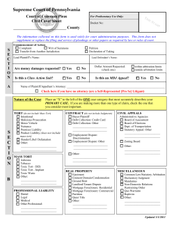


© Copyright 2026