1. sports
2. surfing and bodyboarding

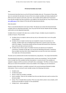
Random Waves in the Laboratory – What is Expected
for the Extremes?
Carl Trygve Stansberg
Norwegian Marine Technology Research Institute A/S (MARINTEK)
P.O.Box 4125 Valentinlyst, N-7046 TRONDHEIM, Norway
[email protected]
Abstract. The generation and interpretation of extreme waves in physical
model testing is discussed. A list of relevant wave parameters describing the
extremes is outlined. A probabilistic approach is considered, with extremes
occurring randomly in a wave train synthesized for the test. Statistical reference
models based on linear and second-order wave theory are applied. Comparisons
to model test results show that the second-order model predicts reasonably well
in most cases, although with a slight under-prediction of steep extremes,
possibly due to unidirectional wave conditions in the laboratory. Under
particular conditions, with narrow-banded unidirectional spectra propagating
more than 12 – 15 wavelengths, special modulation effects may occur in
energetic wave groups, leading to very high extremes that are clearly beyond
second order. This may one possible explanation of “freak waves” observed in
the real ocean. The effect is reflected in th 4th order statistical moment
(kurtosis), and a prediction formula taking this into account is suggested.
1 Introduction
The prediction and reproduction of extreme ocean waves is a complex task, since they
are rare events, and therefore hard to observe in the real ocean. Trying to understand
all the underlying mechanisms, and the resulting physics, can be confusing, since
there may be a number of various conditions leading to the different events actually
observed. Ideally, perfect theoretical and physical models should therefore be able to
cover a broad range of situations. A discussion of the occurrence and prediction of
extreme waves has been given in [1]. Fully nonlinear theoretical models for random
extreme waves do still not exist, although there are several theoretical approaches that
include essential linear and nonlinear components and properties. Thus the challenge
in present day-to-day applications is to sort out which are the most relevant properties
to be modelled, and how to model them. This may vary from application to
application, but there are also general patterns. In the present paper, the generation
and interpretation of wave extremes in physical model testing is discussed.
The laboratory generation of waves has been reviewed in [2]. There are still a
number of questions to be handled in connection with reproduction and use of
extreme wave generation. One of them is: What should we expect – or, in other
words, what is our reference? This question may be two-fold: 1) What is required
from the application?, and 2) what is actually possible, given the laboratory frame?
And furthermore, can we learn something about the wave physics itself from the
experiment? Some key words in this process are:
Parameters selected for reproduction
Input from full scale or theory
Methodology (Stochastic vs. deterministic approach; Synthesisation etc.)
Basic physics vs. laboratory effects
Simplifications
Some practical examples from the experience in an offshore model test basin are
discussed in the paper, on basis of previous presentations in [3], [4]. Here a stochastic
approach is followed, with the synthesisation and physical generation of random
storm records (typically of 3-hours duration, full scale). Thus, the extremes occur as
random events in the scaled wave field, as the result of the random summation of a
large number (thousands) of independent input components. Nonlinear effects
observed in the records are then mainly interpreted as results from nonlinear
couplings in the actual propagation of the laboratory wave field, although one has to
be aware of possible laboratory defined effects. Another approach which has been
suggested and applied in the literature, is the design and use of single deterministic,
transient wave groups specified with particular extreme value properties [5]. The two
different approaches may in certain situations be considered as alternatives to each
other, but it is perhaps more fruitful to treat them as complementary, since they are
based on quite different background philosophies.
The present experimental results are seen in relation to linear and second-order
random wave prediction models, with a particular discussion of deviations from the
models. Thus one possible way of defining “freak waves” may be considered as
waves and crests clearly higher than second-order. A possible connection between
such extremes and nonlinear wave grouping is considered.
2 Background: Critical Wave Events and Parameters
2.1 Some Critical Wave Situations in Offshore Engineering
The design and operation of FPSO’s in extreme weather exposed areas must take into
account the effects from steep and energetic individual wave events. The wave impact
on bow and deck structures can be serious, such as the bow slam experienced on the
Schiehallion FPSO [6], as well as the water on deck problems reported on Norwegian
production vessels [7]. New design tools are being developed as a result of this [8].
The impact loads and possible damages are certainly a combined effect from the wave
properties and the interaction with the vessel, but knowledge about the incoming
energetic waves is very helpful in the further development in the area.
For floating platforms, such as semisubmersibles, TLPs and Spars, the deck
clearance (air-gap) is critical. Thus the ability to properly predict the extreme wave
crests and their kinematics, in 100-year storms is essential, not only for the prediction
of the probability of impact, but also for the prediction of resulting loads. Other direct
results from extreme waves interacting with platforms include the ringing problem on
TLP’s and GBS’s (see e.g. [9], as well as the possible capsizing of platforms with
compliant mooring.
Extreme waves or wave groups can also induce particular vessel motions, as a
result of particularly large slow-drift forces. For FPSO’s, this may lead to large head
angles and, consequently, even larger offset and high nonlinear mooring line loads
(static as well as dynamic). Large slow-drift is critical also for the extreme loads of
platform moorings.
2.2 Critical Wave Parameters
The detailed description of dangerous waves is complex, since the different problems
such as described above may depend on different wave properties. A list of possible
parameters or characteristics may be as follows:
Individual waves
Crest height:
Wave height:
Steepness:
Particle velocity:
Particle acceleration:
Grouping (succeeding waves);
Energy envelope:
Breaking
A max
or
Hmax
or
(∂η/∂x) max or
Umax
(dU/dt)max
A max/σ
Hmax/σ
(kA)max
E(t); Group spectrum – relative to linear model
Short-term sea state properties
Skewness:
γ1 = 1/(M σ3 ) ⋅ Σ [ηi -E(η)]3
Kurtosis (grouping parameter): γ2 = 1/(M σ4 ) ⋅ Σ [ηi -E(η)]4
Probability of given extreme levels
(1)
(2)
where η is the elevation, σ is the standard deviation of the elevation record, and M is
the number of record samples. In addition, there may also be other parameters
relevant for particular problems.
2.3 Extreme Waves: Possible Physical Mechanisms
For a proper prediction of extreme and rare waves, it is also important to keep in mind
that there may be a range of different physical mechanisms leading to the events.
Some of these are:
Phase combination of harmonic components
Steepness-induced crest increase (“Stokes effects”)
Nonlinear self-focusing of energetic wave groups
Multi-directional effects
Bottom effects (finite water depth; refraction)
Current effects (wave-current interaction: refraction)
Wind influence
Storm age and duration
Several storm systems?
Thus the description of real cases may be complex. In offshore engineering
applications, the first two mechanisms listed are perhaps those with most attention. It
may be a reasonable choice to consider them as basic conditions, and then add the
effects from the others when appropriate. Later in this paper, effects from nonlinear
wave grouping are discussed in particular, on basis of some laboratory results.
3 Specification and Limitations of Laboratory Waves
The reproduction of wave conditions in a laboratory must be based upon a chosen
specification, which can be essential for the generated extremes. Thus the reproduced
conditions will be simplified with regard to some properties, while others are
emphasised. Parameters of a specification may include some of the following:
In a probabilistic approach:
Significant wave height
Hs ; Hmo
Spectral peak period (o r equivalent)
Tp ; T z
Spectrum shape (e.g. JONSWAP, 2-peaked etc.)
Storm duration
Additional requirements?
(H max ; A max ; γ1 ; γ2 ; wave grouping; others ?)
In a deterministic transient wave approach:
Specific properties of single wave (or wave group)
Some laboratory simplifications may typically (but not necessarily) be:
Uni-directional waves
Horizontal bottom or deep water
Stationary sea state
Mechanical wave generator - no wind influence
If “transient wave” : Specific parameters of event
Specific laboratory-defined effects:
Reflections & diffraction
“Parasitic waves” due to imperfect boundary conditions
Size & shape of basin / distance from wave generator
Repeatability
Scale effects (viscous effects; breaking)
Synthesization method
4 Proba bilistic Modelling of Linear and Nonlinear Waves
Based on the specification, the synthesisation of a random laboratory signal input to
the wave-maker is typically made as a linear sum of a large number of independent
harmonic components. Nonlinear corrections may also be made [10]. As an example,
a 3-hours storm duration may be simulated by inverse Fast Fourier Transform (FFT)
with 16000 frequency components. Extreme waves are then a result of this random
combination, plus nonlinear interactions during the propagation from the wavemaker
to the actual location. The statistical behaviour is observed through parameters like
the skewness γ1 and kurtosis γ2 of the wave record, and probability distributions and
extremes of the crests and wave heights.
The results can then be compared to reference models. In particular there are two
models in use: Linear waves, with Gaussian statistics and Rayleigh distributed peaks,
and second-order waves [11], [12], with a non-Gaussian correction on the statistics,
and with extreme crests deviating from the Rayleigh model. The effect from secondorder contributions on an extreme wave is shown in a numerical example in Fig. 1.
One should also take into account the sampling scatter of a finite record [12]. The
estimation of extremes from a given 3-hours record can be improved by use of e.g.
fitting the tail of the peak distribution to a Weibull distribution, and predict the
extreme from that.
Fig. 1. Time series sample from numerically generated second-order random wave
Based on the reference models, we can derive expectations for the measured statistics,
and the extremes in particular. For a simple linear model, the expected skewness and
kurtosis are γ1 = 0; γ2 = 3.0, respectively, and extreme crests and wave heights are
expected to be Rayleigh distributed with the following commonly used relations:
E[A max] ≡ A R = σ [√ (2 ln (M)) + 0.577/√ (2 ln (M))]
E[Hmax] = 2 A R
(3)
(4)
In a second-order model, the skewness γ1 increases linearly with the steepness.
Models for γ1 and γ2 have been derived in [13]:
γ1 = 5.41 (Hm0 / L p )
γ2 – 3 = 3 γ1 2
(5)
(6)
where L p is the wavelength corresponding to the peak wave period. For extreme
crests a simplified formula has been proposed by [14]:
E[A max] = A R (1 + ½ kp A R )
(7)
where kp is the wave number corresponding to L p , and A R is given in Eq. (3) above.
The wave heights are still Rayleigh distributed as in the linear model.
The experience from [11] is that the second-order model generally agrees quite
well with deep water full scale measurements of crests. Thus the linear model will
underpredict extreme crests but not the wave heights. Laboratory measurements in [3]
more or less confirm this (see the next chapter), but a slight under-prediction is
observed. In special conditions, even higher extremes have been observed [4]. Higherorder models can also predict this [15]. Such events may possibly be seen in relation
to full-scale observations of so-called “freak waves”, and will be discussed later in
this paper.
5 Observed Nonlinear Behaviour of Random Extremes
Observations from a range of model test studies in scales 1:55 – 1:70, with random
wave generation in a large wave basin [3], have shown that the largest crest heights
deviate systematically from Rayleigh model predictions derived for linear waves. In
general, a second-order description fits reasonably well, as concluded from the fullscale study in [11], although it slightly under-predicts the most extreme cases,
typically by 5% of the total crests. See Fig. 2. The deviation may be partly due to the
fact that most of the results in this figure were obtained with unidirectional waves,
while field data are expected to be more or less muliti-directional. There is a also a
considerable sampling scatter, as expected from theory. Extreme peak -to-peak wave
heights are normally reasonably well predicted by Rayleigh theory. The same results
are also reflected in probability distributions (Fig. 3).
Fig.2. Measured extreme crests from laboratory tests, compared to second-order and Rayleigh
predictions. 3-hours as well as 12 – 18-hours storm duration models (from Stansberg, 2000a)
Fig.3a. Probability distributions of crests in 1:55 scaled 18-hours storm model test
Fig. 3b. As Fig. 3a, but for wave heights.
Under certain conditions, extremes in random wave trains may be observed to be
significantly higher than second-order predictions, even for moderately steep wave
conditions [4]. This occurs when unidirectional, narrow-banded spectra propagate
over large distances, that is, more than about 12-15 wavelengths, in which case
higher-order wave group amplification may take place, leading to particularly high
crests and wave heights. This is illustrated by an example from a 1:200 scaled
laboratory experiment shown in Fig.4. We may interpret it as a so-called “freak wave”
event. However, the results in [4] also show that it can be a result of systematic
behaviour under these particular conditions. A reasonable physical explanation is the
self-focusing casued by amplitude dispersion in energetic wave groups, which can be
related to the modulational instabilities commonly referred to as the Benjamin -Feir
effect [16]. The physics is studied experimentally in [17]. Results from tests with
different scales indicate that the phenomenon is not scale dependent. For bi-chromatic
wave trains, observations have been found to agree very well with a higher-order
Schrödinger formulation [18]. Probability crest and height distributions from a case
where the effect is particularly strong are shown in Fig 5. The difference from Fig. 3
above is clearly seen, also for the peak-to-peak wave heights.
The 4th -order statistical moment parameter γ2 (kurtosis) reflects, on an average, the
increased groupiness, although it is also statistically unstable [12]. An empirical
relation has been derived on basis of the experimental data above, with very
Fig. 4. Space and time evolution of energetic wave group into extreme wave – example from
model tests. (D = distance from wave-maker, in wavelengths))
long records corresponding to 12, 15, 18 and 36 hour storm models. Thus the kurtosis
has been correlated with the corresponding 3-hours extreme crest and wave height
estimates Amax , Hmax. The result is shown in Fig. 6, where deviations from the
second-order and Rayleigh models (for Amax and Hmax , respectively) are plotted
against the kurtosis. The values are normalised by the standard deviation σ of the
record. From this, the following simplified formulae are proposed for extreme crests
and wave heights, taking into account the second-order term for A max [16] as well as
an empirical higher order correction for A max and for Hmax:
A max / σ = (A max,R / σ)⋅ (1 + ½ kp A max,R ) + 1.3⋅ (γ2 - 3.0)
(8)
Hmax /2σ = (Hmax,R /2σ) + (γ2 - 3.25)
(9)
We sees that for the extreme wave heights, the Rayleigh model overpredicts the
measurements when the kurtosis approaches 3.0 (that is, Gaussian waves). This is an
expected result in linear waves, due to the de-correlation between crests and
neighbouring troughs in a finite-bandwidth spectrum.
Fig. 5. Probability distributions of crests and wave heights, after 25 wavelengths
Fig. 6. Measured extreme crests and wave heights in 12 – 36 hours storm tests: Deviations
from second-order and Rayleigh models, respectively, vs. kurtosis
Another, more general alternative to this empirical formula is the Hermite
transformation method in [19]), where the extremes are estimated directly on basis of
the statistical moments γ1 and γ2 .
The kurtosis γ2 will have to be determined for the actual case. Thus there is a task
for the future: How do we know when to assume γ2 clearly larger than 3.0 , and how
do we predict it?
The typical time domain behaviour of the most extreme (“freak”) events is shown
in Fig. 7. It normally results from an energetic wave group of 4-6 waves, which after
some propagation is focused into a narrower group of of 1-2 waves. Most of the
energy is then concentrated in the front wave. Until this point, only little energy has
been dissipated from the original wave group. Thus the occurrence of such “freak”
events may possibly be caused by the time and space development of wave groups
with a duration sufficient to contain a large amount of integrated energy.
6 Conclusions
Probabilistic modelling of storm sea states in a laboratory wave basin, with
particular emphasis on the resulting extreme wave events, has been discussed and
demonstrated. The results are seen in light of what is expected from linear and second
Fig. 7. Particularly extreme wave event.
order models. Main findings are:
An empirically adjusted formula for extremes is suggested. For the crests, this is
based on a second-order model plus an empirical correction for kurtosis values larger
than 3.0. For the wave heights, a Rayleigh model with a similar kurtosis correction is
proposed.
The kurtosis is closely connected with the average “groupiness” of the sea state.
Normally it is 3.0 – 3.2, but it can under certain conditions, such as narrow-banded,
unidirectional sea on deep water, grow significantly higher.
Nonlinear group amplification (focusing) can generate strongly nonlinear, rare
wave events – clearly beyond second order
There is a considerable sampling variability in a randomly chosen 3-hours
realisation, as expected from theory.
References
1. ISSC, Report from the 23rd International Ships and Structures Conference - Environment
Committee, Nagasaki, Japan (2000).
2. ITTC, Report from the 22nd International Towing Tank Conference - Environment
Committee, Seoul, Korea and Shanghai, China (1999).
3. Stansberg, C.T.: Laboratory Reproduction of Extreme Waves in a Random Sea, Proc., Wave
Generation'99 (International Workshop on Natural Disaster by Storm Waves and Their
Reproduction in Experimental Basin), Kyoto, Japan, (2000).
4. Stansberg, C.T.: Nonlinear Extreme Wave Evolution in Random Wave Groups, Proc., Vol.
III, the 10th ISOPE Conf., Seattle, WA, USA, (2000).
5. Clauss, G.: Task-Related Wave Groups for Seakeeping Tests or Simulation of Design Storm
Waves, Appl. Ocean Res., Vol. 21, (1999), pp. 219-234.
6. MacGregor, J.R., Black, F., Wright, D. and Gregg, J.: Design and Construction of the FPSO
Vessel for the Schiehallion Field, Trans., Royal Inst. of Naval Architects, London, UK,
(2000).
7. Ersdal, G. and Kvitrud, A.: Green Water on Norwegian Production Ships, Proc., the 10th
ISOPE Conf., Seattle, WA, USA, (2000).
8. Hellan, Ø., Hermundstad, O.A. and Stansberg, C.T.: Design Tool for Green Sea, Wave
Impact and Structural Responses on Bow and Deck Structures, OTC Paper No. 13213, OTC
2001 Conference, Houston, TX, USA, (2001).
9. Davies, K.B., Leverette, S.J. and Spillane, M.W.: Ringing Response of TLP and GBS
Platforms, Proc. Vol. II, the 7th BOSS Conf., Cambridge, Mass., USA, (1994).
10. Schäffer, H.A.: Second-Order Wavemaker Theory for Irregular Waves, Ocean Engr, 23,
No. 1, (1996), 47-88.
11. Forristall, G.: Wave Crest Distributions: Observations and Second-Order Theory, Proc.,
Conf. On Ocean Wave Kinematics, Dynamics, and Loads on Structures, Houston, TX, USA,
(1998), 372-382.
12. Stansberg, C.T.: Non-Gaussian Extremes in Numerically Generated Second-Order Random
Waves in Deep Water, Proc., Vol. III, the 8th ISOPE Conf., Montreal, Canada, (1998), 103110.
13. Vinje, T. and Haver, S.: On the Non-Gaussian Structure of Ocean Waves, Proc., Vol. 2, the
7th BOSS Conf., MIT, Cambridge, Mass., USA. (Published by Pergamon, Oxford, UK,
(1994).
14. Kriebel, D.L. and Dawson, T.H.: Nonlinearity in Wave Crest Statistics, Proc., 2nd Int Symp
on Wave Measurement and Analysis, New Orleans, LA, USA, (1993), 61-75.
15. Yasuda, T. and Mori, N.: High Order Nonlinear Effects on Deep-Water Random Wave
Trains, Proc., Vol. II, Int Symp on Waves – Phys. and Num. Modelling, Univ. of British
Columbia, Vancouver, Canada, (1994), 823 – 832.
16. Benjamin, T.B. and Feir, J.E.: The Disintegration of Wave Trains on Deep Water, J. Fluid
Mech., Vol. 27, (1967), 417-430.
17. Stansberg, C.T.: On the Nonlinear Behaviour of Ocean Wave Groups, Proc. WAVES 1997
Symposium (ASCE), Virginia Beach, VA, USA, (1998).
18. Trulsen, K. and Stansberg, C.T.: Spatial Evolution of Water Surface Waves: Numerical
Simulation and Experiment of Bichromatic Waves, Proc., the 11th ISOPE Conf., Stavanger,
Norway, (2001).
19. Winterstein, S.R.: Nonlinear Vibration Models for Extremes and Fatigue, J. Eng. Mech.,
Vol. 114, (1988), 1772-1790.