
SPHERE PACKING BOUNDS VIA SPHERICAL CODES
SPHERE PACKING BOUNDS VIA SPHERICAL CODES
HENRY COHN AND YUFEI ZHAO
Abstract. The sphere packing problem asks for the greatest density of a
packing of congruent balls in Euclidean space. The current best upper bound
in all sufficiently high dimensions is due to Kabatiansky and Levenshtein in
1978. We revisit their argument and improve their bound by a constant factor
using a simple geometric argument, and we extend the argument to packings
in hyperbolic space, for which it gives an exponential improvement over the
previously known bounds. Additionally, we show that the Cohn-Elkies linear
programming bound is always at least as strong as the Kabatiansky-Levenshtein
bound; this result is analogous to Rodemich’s theorem in coding theory. Finally,
we develop hyperbolic linear programming bounds and prove the analogue of
Rodemich’s theorem there as well.
1. Introduction
What is the densest arrangement of non-overlapping, congruent balls in Rn ? This
problem has a long history and has been extensively studied [CS99], and it has
strong connections with physics and information theory [C10]. With the proof of
Kepler’s conjecture by Hales [H05], the sphere packing problem has been solved in
up to three dimensions, but no proof of optimality is known in any higher dimension,
and there are only a few dozen cases in which there are even plausible conjectures
for the densest packing. In R8 and R24 there are upper bounds that are remarkably
close to the densities of the E8 and Leech lattices, respectively; for example, Cohn
and Kumar [CK04, CK09] came within a factor of 1 + 10−14 of the density of E8
and a factor of 1 + 1.65 · 10−30 of the density of the Leech lattice. However, in most
dimensions we must be content with much cruder bounds. In this paper, we will
slightly improve the best upper bounds known in high dimensions, show how to
obtain them via linear programming bounds, and extend them to hyperbolic space.
The density of a sphere packing in Rn is the fraction of space covered by the
n
balls in the packing. More precisely, let BR
(x) denote the ball of radius R centered
n
at x; then the density of a packing is the limit as R → ∞ of the fraction of BR
(x)
covered by the packing (the limit is independent of x if it exists). Of course this
limit need not exist, but one can replace it with the upper density defined with a
limit superior, and one can show that the least upper bound of the upper densities
of all sphere packings in Rn is actually achieved as the density of a packing (see
[G63]). Let ∆Rn denote this maximal packing density.
A spherical code in dimension n with minimum angle θ is a set of points on the
unit sphere in Rn with the property that no two points subtend an angle less than
θ at the origin. In other words, hx, yi ≤ cos θ for all pairs of distinct points x, y in
the spherical code. Let A(n, θ) denote the greatest size of such a spherical code.
Date: November 14, 2013.
Zhao was supported by an internship at Microsoft Research New England.
1
2
HENRY COHN AND YUFEI ZHAO
In this paper, we consider the problem of finding upper bounds for packing
density. Linear programming bounds have proven to be a powerful tool. This
technique was first developed by Delsarte [D72] in the setting of error-correcting
codes, and his method can be extended to many other settings. In particular,
Delsarte, Goethals, and Seidel [DGS77] and Kabatiansky and Levenshtein [KL78]
independently formulated a linear program for proving upper bounds on A(n, θ).
Using this approach, Kabatiansky and Levenshtein found excellent upper bounds on
A(n, θ) for large n, and they then applied a geometric argument to deduce a bound
on ∆Rn . Their upper bound is currently the best bound known for n ≥ 115 (see
Appendix A). It has the asymptotic form
(1.1)
∆Rn ≤ 2−(0.5990...+o(1))n ,
while the best lower bound known remains 2−(1+o(1))n despite recent improvements
[V11, V13].
Cohn and Elkies [CE03] found a more direct approach to bounding sphere packing
densities, with no need to consider spherical codes. Their technique set new records
in every case with n ≥ 4 for which the calculations were carried out; see Appendix A
for more details, and see Theorem 1.4 in [LOV12] for subsequent improvements
when n = 4, 5, 6, 7, and 9. However, despite the evidence from low dimensions,
the asymptotic behavior of the Cohn-Elkies bound is far from obvious and it has
been unclear whether it improves on, or even matches, the Kabatiansky-Levenshtein
bound asymptotically. Until this paper, it was only known how to use the CohnElkies linear program to match the “second-best bound” by Levenshtein [L79] (see
Section 6 of [CE03]).
The purpose of this paper is fourfold. In Section 2 we improve the KabatianskyLevenshtein bound by a constant factor by giving a simple modification of their
geometric argument relating spherical codes to sphere packings. (This does not
change the exponential decay rate in bound (1.1)). In Section 3 we show that in every
dimension n, the Cohn-Elkies linear program can always match the KabatianskyLevenshtein approach. This further demonstrates the power of the linear programming bound for sphere packing. In Section 4 we prove an analogue of the
Kabatiansky-Levenshtein bound in hyperbolic space. The resulting bound behaves
the same as (1.1) asymptotically, and it is exponentially better than the best bound
previously known in hyperbolic space. Finally, in Section 5, we develop the theory of
hyperbolic linear programming bounds (based partly on unpublished work of Cohn,
Lurie, and Sarnak) and prove that they too subsume the Kabatiansky-Levenshtein
approach.
2. Geometric argument
In all sufficiently high dimensions, the best upper bound currently known for
sphere packing density is given by Kabatiansky and Levenshtein [KL78] (see also
Chapter 9 of [CS99] and Chapter 8 of [Z99]). They first obtain an upper bound on
A(n, θ) using linear programming and then use the inequality
(2.1)
∆Rn ≤ sinn (θ/2)A(n + 1, θ).
The inequality was derived using a simple geometric argument. Here we improve it
using an equally simple argument.
SPHERE PACKING BOUNDS VIA SPHERICAL CODES
3
Figure 1. Proof of Proposition 2.1.
Proposition 2.1. For all n ≥ 1 and π/3 ≤ θ ≤ π,
(2.2)
∆Rn ≤ sinn (θ/2)A(n, θ).
Since the unit sphere in Rn can be embedded in the unit sphere in Rn+1 via a
hyperplane through the origin, we always have A(n, θ) ≤ A(n + 1, θ), with strict
inequality when θ ≤ π/2. The applications of (2.1) have π/3 ≤ θ ≤ π/2, so
Proposition 2.1 will be a strict (though small) improvement. Neither inequality is
useful in low dimensions; for example, when n = 2 and θ = π/3, Proposition 2.1
says that ∆R2 ≤ 3/2. However, these inequalities are valuable in high dimensions.
For the sake of comparison, let us first recall the proof of (2.1).
Proof of (2.1). Suppose we have a sphere packing in Rn of density ∆ using unit
n
spheres. Consider a sphere SR
in Rn+1 of radius R (to be chosen later), and place
n
n
the sphere packing in R onto a hyperplane through the center of SR
, with the
n
n
packing translated so that at least ∆R of the sphere centers are contained in SR
.
This is always possible by an averaging argument: a randomly chosen translation
n
will lead to an average of ∆Rn sphere centers in SR
. Project the sphere centers
n
onto the upper hemisphere of SR , orthogonally to the hyperplane. The projections
of the sphere centers are still at least distance two apart, and thus separated by
angles of at least θ, where sin(θ/2) = 1/R. Therefore, ∆Rn ≤ A(n + 1, θ), which is
the bound that we wanted to prove, and we can achieve any angle by choosing R
accordingly.
Our motivation for revisiting this argument is that it feels somewhat unnatural
to lift to a higher dimension in the process. Our proposition shows that a stronger
inequality can be obtained without going to a higher dimension. The proof is similar
to the techniques of [HST10] and [BM07], but this application appears to be new.
Proof of Proposition 2.1. See Figure 1. Suppose we have a packing of unit spheres
n−1
in Rn with density ∆. Let SR
be a sphere in Rn of radius R ≤ 2 (to be chosen
later), located so that it contains at least ∆Rn of the centers of the spheres in the
packing but its center is not one of them. Such a location always exists, by the
same averaging argument as above (a randomly chosen location will contain an
average of ∆Rn sphere centers). Now, project the sphere centers from the packing
n−1
n−1
onto the surface of SR
using rays starting from the center of SR
. It follows
from the lemma below that the projections are separated by angles of at least θ,
where sin(θ/2) = 1/R. Therefore, ∆Rn ≤ A(n, θ), as desired, and we can achieve
any angle of π/3 or more using R ≤ 2.
4
HENRY COHN AND YUFEI ZHAO
Z
X
Y
Figure 2. Pictorial proof of Lemma 2.2. The bounds |XZ| ≤ R
and |Y Z| ≤ R place Z in the dark gray region, which is the
intersection of the two disks centered at X and Y with radius R ≤ 2.
The light gray region contains all points P with ∠XP Y ≥ θ. Since
the dark region is contained inside the light region, it follows that
∠XZY ≥ θ.
Note that the proof breaks down if R > 2, because two projected sphere centers
can even coincide.
Lemma 2.2. Suppose R ≤ 2. If XY Z is a triangle with |XY | ≥ 2, |XZ| ≤ R,
|Y Z| ≤ R, then ∠XZY ≥ θ, where sin(θ/2) = 1/R.
Proof. See Figure 2 for a pictorial proof. For an algebraic proof, let x = |XZ|, y =
|Y Z|, z = |XY |, and γ = ∠XZY . By the law of cosines, cos γ = (x2 +y 2 −z 2 )/(2xy).
By taking partial derivatives, we see that the expression (x2 + y 2 − z 2 )/(2xy) is
maximized in the domain 0 ≤ x, y ≤ R and z ≥ 2 at (x, y, z) = (R, R, 2). Therefore,
cos γ ≤ 1 − 2R−2 = 1 − 2 sin2 (θ/2) = cos θ. It follows that γ ≥ θ.
Inequalities (2.1) and (2.2) can be stated a little more naturally in terms of
packing density on the sphere. A spherical code on S n−1 with minimal angle θ and
size A(n, θ) corresponds to a packing with spherical caps of angular radius θ/2 with
density
R θ/2 n−2
sin
x dx
(2.3)
A(n, θ) R0 π n−2
.
sin
x dx
0
In other words, it covers this fraction of the sphere. Now if we let ∆S n−1 (θ) denote
the optimal packing density, then (2.2) implies
(2.4)
1
1
log ∆Rn . log ∆S n−1 (θ),
n
n
where f (n) . g(n) means f (n) ≤ h(n) for some function h with h(n) ∼ g(n) (i.e.,
limn→∞ h(n)/g(n) = 1). This simply amounts to verifying that
R θ/2 n−2
sin
x dx
1
θ
log R0 π n−2
∼ log sin
n
2
sin
x dx
0
for fixed θ satisfying 0 < θ ≤ π. Furthermore, it is known that
(2.5)
1
1
log ∆S n−1 (θ) .
log ∆S n (φ)
n
n+1
SPHERE PACKING BOUNDS VIA SPHERICAL CODES
5
for 0 < θ < φ ≤ π/2 (see (17) in [L75]). Thus, the exponential rate of the packing
density for spherical caps is weakly increasing as a function of angle, and Euclidean
space naturally occurs as the zero angle limit.
The proof of the Kabatiansky-Levenshtein bound (1.1) on ∆Rn uses the following
bound on A(n, θ) for 0 < θ < π/2, which is derived using the linear programming
bound for spherical codes (see Theorem 4 in [KL78]):
(2.6)
1
1 + sin θ
1 + sin θ 1 − sin θ
1 − sin θ
log A(n, θ) .
log
−
log
.
n
2 sin θ
2 sin θ
2 sin θ
2 sin θ
The bound (1.1) is then deduced by setting (2.6) into (2.1) and choosing θ to
minimize the resulting bound,1 which turns out to happen at θ = 1.0995 . . . ≈ 0.35π.
If we now apply our new inequality (2.2) in place of (2.1), then we obtain an
improvement in the bound by a factor of An+1 /An , where An = (1.2635 . . . + o(1))n
is the Kabatiansky-Levenshtein bound on A(n, 1.0995 . . .). Thus, we obtain an
improved sphere packing bound by a factor of 1.2635 . . . on average, in the sense
that the geometric mean of the improvement factors over all dimensions from 1 to
N tends to 1.2635 . . . as N → ∞.
3. Linear programming bounds
In [KL78] the upper bound on the maximum sphere packing density ∆Rn was
derived by first giving an upper bound for the maximum size A(n, θ) of a spherical
code using linear programming, and then using (2.1) to compare the two quantities.
We refer to this method as the Kabatiansky-Levenshtein approach. Cohn and Elkies
[CE03] took a more direct approach to bounding ∆Rn , by setting up a different
linear program. In this section, we show that the Cohn-Elkies linear program can
always prove at least as strong a bound on ∆Rn as the Kabatiansky-Levenshtein
approach.
This theorem is the continuous analogue of a theorem of Rodemich [R80] in
coding theory (see Theorem 3.5 of [D94] for a proof of Rodemich’s theorem, since
Rodemich published only an abstract). Let A(n, d) denote the maximum size of a
binary error-correcting code of block length n and minimal Hamming distance d
n
(i.e., a subset of {0, 1} with every two elements differing in at least d positions),
and let A(n, d, w) denote the maximum size of such a code with constant weight w
(i.e., every element of the subset has exactly w ones). The current best bounds on
A(n, d) and A(n, d, w) for large n are by McEliece, Rodemich, Rumsey, and Welch
[MRRW77], using linear programming bounds. As in the Kabatiansky-Levenshtein
approach, some of the best bounds on A(n, d) were obtained using bounds on
A(n, d, w) along with an analogue of Proposition 2.1 known as the Bassalygo-Elias
inequality [B65]:
(3.1)
A(n, d) ≤
2n
n A(n, d, w).
w
1Let us clarify a potentially confusing point. The fact that θ = 1.0995 . . . minimizes the bound
may, at first, seem to be at odds with (2.4) and (2.5), where we said that the exponential rate of
the packing density ∆S n−1 (θ) is weakly increasing in θ. Both statements are correct. The bound
in (2.6) is a preliminary bound on A(n, θ), which can be improved for θ less than the critical
value 1.0995 . . . by incorporating (2.5). This improvement yields the same bound on ∆Rn for all
θ ≤ 1.0995 . . ..
6
HENRY COHN AND YUFEI ZHAO
The proof of (3.1) is by an easy averaging argument. In analogy with sphere packing,
error-correcting codes play the role of sphere packings while constant weight codes
play the role of spherical codes. Rodemich proved that any upper bound on A(n, d)
obtained using the linear programming bound for A(n, d, w) combined with (3.1)
can be obtained directly via the linear programming bound for A(n, d). Theorem 3.4
below is the continuous analogue of Rodemich’s theorem.
3.1. LP bounds for spherical codes. We begin by reviewing the linear programming bounds for spherical codes. We follow the approach of Kabatiansky and
Levenshtein [KL78], based on their inequality on the mean.
Let S n−1 denote the unit sphere in Rn . A function f : [−1, 1] → Ris positive
definite if for all N and all x1 , . . . , xN ∈ S n−1 , the matrix f (hxi , xj i) 1≤i,j≤N is
positive semidefinite. (Note that this property depends on the choice of n; when
necessary for clarity, we will say such a function is positive definite on S n−1 .)
Equivalently, for all x1 , . . . , xN ∈ S n−1 and t1 , . . . , tN ∈ R,
X
ti tj f (hxi , xj i) ≥ 0.
1≤i,j≤N
A result of Schoenberg [S42] characterizes continuous positive-definite functions
n/2−1
as the nonnegative linear combinations of the Gegenbauer polynomials Ck
for
α
k = 0, 1, 2, . . . . Recall that the polynomials Ck are orthogonal with respect to the
measure (1 − t2 )α−1/2 dt on [−1, 1]. When α = n/2 − 1, this measure arises naturally
(up to scaling) as the orthogonal projection of the surface measure from S n−1 onto
a coordinate axis.
Given a positive-definite function g, define g to be its average
R1
g(t)(1 − t2 )(n−3)/2 dt
g = −1
R1
(1 − t2 )(n−3)/2 dt
−1
with respect to this measure. Equivalently, g is the expectation of g(hx, yi) with x
and y chosen independently and uniformly at random from S n−1 . If
X
n/2−1
g(t) =
ck Ck
(t),
k≥0
then g = c0 .
Theorem 3.1 (Delsarte-Goethals-Seidel [DGS77], Kabatiansky-Levenshtein [KL78]).
If g : [−1, 1] → R is continuous and positive definite on S n−1 , g(t) ≤ 0 for all
t ∈ [−1, cos θ], and g > 0, then
A(n, θ) ≤
g(1)
.
g
Let ALP (n, θ) denote the best upper bound on A(n, θ) that could be derived using
Theorem 3.1. In other words, it is the infimum of g(1)/g over all valid auxiliary
functions g.
We will give a proof of this theorem following the approach of [KL78], as preparation for giving a new proof of Theorem 3.3 below.
Proof. Let C be any spherical code in S n−1 with minimal angle at least θ, let µ be
the surface measure on S n−1 , normalized to have total measure 1, let δx be a delta
SPHERE PACKING BOUNDS VIA SPHERICAL CODES
7
function at the point x, and let
ν=
X
δx + λµ,
x∈C
where λ is a constant to be determined. We have
ZZ
g(hx, yi) dν(x) dν(y) ≥ 0,
because we can approximate the integral with a sum and use the positive definiteness
of g. This inequality amounts to
X
λ2 g + 2λ|C|g +
g(hx, yi) ≥ 0.
x,y∈C
Because hx, yi ≤ cos θ for distinct points x, y ∈ C and g(t) ≤ 0 for t ∈ [−1, cos θ], we
have
X
X
g(hx, yi) ≤
g(hx, xi) = |C|g(1).
x,y∈C
x∈C
Thus,
λ2 g + 2λ|C|g + |C|g(1) ≥ 0.
To derive the best bound on |C|, we take λ = −|C|. Then
0 ≤ −|C|2 g + |C|g(1)
and hence
|C| ≤
as desired.
g(1)
,
g
3.2. LP bounds in Euclidean space. The Kabatiansky-Levenshtein approach
gives the following bound on ∆Rn . The original version uses (2.1), but here we state
the improved version using Proposition 2.1.
Corollary 3.2. Suppose g satisfies the hypotheses of Theorem 3.1 with π/3 ≤ θ ≤ π.
Then
g(1)
∆Rn ≤ sinn (θ/2)
.
g
Let us recall the Cohn-Elkies linear programming bound. Given an integrable
function f : Rn → R, let fb denote its Fourier transform, normalized by
Z
fb(t) =
f (x)e2πihx,ti dt.
Rn
n
BR
Let
denote the n-dimensional ball with radius R. The volume of the ndimensional unit ball is vol(B1n ) = π n/2 /(n/2)!, where (n/2)! = Γ(n/2 + 1) for
n odd.
Much like the case of spheres, a function f : Rn →
R is positive definite if for all
N and all x1 , . . . , xN ∈ Rn , the matrix f (xi − xj ) 1≤i,j≤N is positive semidefinite.
A result of Bochner [B33] characterizes continuous positive-definite functions as the
Fourier transforms of finite Borel measures. If f and fb are both integrable, then f
is positive definite if and only if fb is nonnegative everywhere, by Fourier inversion
and Bochner’s theorem.
8
HENRY COHN AND YUFEI ZHAO
Theorem 3.3 (Cohn-Elkies [CE03]). Suppose f : Rn → R is continuous, positive
definite, and integrable, f (x) ≤ 0 for all |x| ≥ 2, and fb(0) > 0. Then
∆Rn ≤ vol(B1n )
f (0)
.
fb(0)
The original version in [CE03] required suitable decay of f and fb at infinity,
and it was based on Poisson summation. These more restrictive hypotheses were
removed in Section 9 of [CK07]. Here we give a more direct proof, although it has
the disadvantage of not telling as much about what happens when equality holds as
the Poisson summation proof does.
Proof. Without loss of generality, we can symmetrize to assume f is an even function
(indeed, radially symmetric). This is not necessary for the proof, but it will simplify
some of the expressions below.
Let P be a packing with balls of radius 1, such that P has density ∆Rn . Given a
radius r > 0, let Sr be the set of sphere centers from P that lie within the ball of
radius r about the origin, let Vr be the volume of that ball, and let Nr = |Sr |. Then
Nr
lim vol(B1n )
= ∆Rn .
r→∞
Vr
√
√
Let R = r + r (in fact, r could be replaced with any function that tends to
infinity but is o(r)). Consider the signed measure
X
ν=
δx + λµR ,
x∈Sr
where δx is the delta function at x, µR is Lebesgue measure on the ball of radius
R centered at the origin, and λ is a constant to be determined. As in the proof of
Theorem 3.1,
ZZ
f (x − y) dν(x) dν(y) ≥ 0,
because f is positive definite. Equivalently,
ZZ
XZ
2
λ
f (x − y) dx dy + 2λ
|x|,|y|≤R
x∈Sr
X
f (x − y) dy +
|y|≤R
f (x − y) ≥ 0.
x,y∈Sr
Because f (x − y) ≤ 0 whenever x and y are distinct points in the packing,
ZZ
XZ
2
λ
f (x − y) dx dy + 2λ
f (x − y) dy + Nr f (0) ≥ 0.
|x|,|y|≤R
x∈Sr
|y|≤R
Assuming r is large enough that Nr > 0, we set λ = −Nr /Vr and divide by Nr to
obtain
ZZ
Z
Nr 1
Nr 1 X
·
f (x − y) dx dy − 2 ·
·
f (x − y) dy + f (0) ≥ 0.
Vr Vr
V r Nr
|x|,|y|≤R
|y|≤R
x∈Sr
It is not hard to compute the limits
ZZ
1
lim
f (x − y) dx dy = fb(0)
r→∞ Vr
|x|,|y|≤R
and
Z
1 X
f (x − y) dy = fb(0).
r→∞ Nr
|y|≤R
lim
x∈Sr
SPHERE PACKING BOUNDS VIA SPHERICAL CODES
9
Specifically, when |x| ≤ r, the y-integral covers all values of x − y up to radius
√
R − r = r. As r → ∞ these y-integrals converge to fb(0), and all but a negligible
fraction of the values of x satisfying |x| ≤ R also satisfy |x| ≤ r.
Thus, in the limit as r → ∞ we find that
∆R n b
∆R n b
f (0) − 2
f (0) + f (0) ≥ 0,
n
vol(B1 )
vol(B1n )
which is equivalent to the desired inequality.
Let ∆LP
Rn denote the optimal upper bound on ∆Rn using Theorem 3.3. Recall that
A (n, θ) denotes the optimal upper bound on A(n, θ) obtained using Theorem 3.1.
Our next result compares the LP bound on the sphere packing density ∆Rn obtained
from Corollary 3.2 with the one from Theorem 3.3.
LP
Theorem 3.4. For π/3 ≤ θ ≤ π and positive integers n,
n
LP
∆LP
(n, θ).
Rn ≤ sin (θ/2)A
To prove Theorem 3.4, we will show that for any upper bound on ∆Rn obtained
using a function g in Corollary 3.2, we can always find a function f that gives a
matching bound using Theorem 3.3. In other words,
sinn (θ/2)
g(1)
f (0)
= vol(B1n )
.
g
fb(0)
We have a similar conclusion for the original Kabatiansky-Levenshtein bound
using (2.1) without the θ ≥ π/3 assumption. See the remarks following the proof.
Proof of Theorem 3.4. Let g be any function satisfying the hypotheses of Theorem 3.1. The idea is to construct a function f : Rn → R based on g mimicking the
geometric argument in the proof of Proposition 2.1. Let R = 1/ sin(θ/2), as in that
proof.
Consider the integral
Z
x−z y−z
,
g
dz,
n (x)∩B n (y)
|x − z| |y − z|
BR
R
n
(x) is the ball of radius R centered at x. Note that
where BR
x−z y−z
,
= cos ∠xzy,
|x − z| |y − z|
where ∠xzy denotes the angle at z formed by x and y. This angle is not defined if
x = z or y = z, but these cases occur with measure zero.
The integral depends only on |x − y|, so there is a radial function f : Rn → R
satisfying
Z
x−z y−z
f (x − y) =
g
,
dz.
n (x)∩B n (y)
|x − z| |y − z|
BR
R
We claim that f is positive definite. Indeed, let χR denote the characteristic function
n
of BR
(0). Then we can rewrite f as
Z
x−z y−z
f (x − y) =
χR (x − z)χR (y − z) g
,
dz.
|x − z| |y − z|
Rn
10
HENRY COHN AND YUFEI ZHAO
For any x1 , . . . , xN ∈ Rn and t1 , . . . , tN ∈ R, we can expand
X
ti tj f (xi − xj )
1≤i,j≤N
as
Z
X
(ti χR (xi − z))(tj χR (xj − z)) g
Rn 1≤i,j≤N
xi − z xj − z
,
|xi − z| |xj − z|
dz.
This expression is nonnegative, because g is positive definite on the unit sphere in
Rn and we can use ti χR (xi − z) as coefficients. This shows that f is positive definite
on Rn . It is also integrable, because it has compact support (it vanishes past radius
2R).
If |x − y| ≥ 2, then by Lemma 2.2,
x−z y−z
,
≤ cos θ
|x − z| |y − z|
n
n
for all z ∈ BR
(x) ∩ BR
(y) \ {x, y}. Since g(t) ≤ 0 for all t ∈ [−1, cos θ] by hypothesis,
it follows that f (x − y) ≤ 0 whenever |x − y| ≥ 2. Thus, we have verified that f
satisfies all the hypotheses of Theorem 3.3 except fb(0) > 0, which we will check
n
shortly. We have f (0) = vol(BR
)g(1) and
Z
fb(0) =
f (x − 0) dx
n
ZR Z
x − z −z
=
χR (x − z)χR (−z) g
,
dx dz
|x − z| |−z|
Rn Rn
Z Z
u v
=
χR (u)χR (v) g
,
du dv
|u|
|v|
n
n
R
R
n 2
= vol(BR
) g.
Therefore fb(0) > 0 and
vol(B1n )
as desired.
n
f (0)
) g(1)
1 g(1)
g(1)
vol(BR
= n
= sinn (θ/2)
,
= vol(B1n )
n )2 g
b
vol(B
R
g
g
f (0)
R
When θ < π/3 we can similarly match the Kabatiansky-Levenshtein bound
obtained using (2.1) by adapting the above proof for the corresponding geometric
argument. Let π : B1n → {x ∈ S n : xn+1 ≥ 0} denote the map that orthogonally
projects the unit disk in the hyperplane Rn × {0} in Rn+1 to the upper half of the
unit sphere in Rn+1 . For any g in Theorem 3.1 that gives a bound for A(n + 1, θ),
let
Z
y−z
x−z
,π
dz.
f (x − y) =
g
π
n (x)∩B n (y)
R
R
BR
R
A similar argument shows that f is positive definite and f (x) ≤ 0 whenever |x| ≥ 2.
n
n 2
We have f (0) = vol(BR
)g(1) and fb(0) = vol(BR
) E[g(hπ(u), π(v)i)], where u and
v are independent uniform random points in B1n . The inequality on the mean
from [KL78] says that the average of a positive-definite kernel with respect to a
SPHERE PACKING BOUNDS VIA SPHERICAL CODES
11
probability distribution on its inputs must be at least as large as that with respect
to the uniform distribution. Thus, E[g(hπ(u), π(v)i)] ≥ g and
vol(B1n )
g(1)
f (0)
≤ sinn (θ/2)
.
b
g
f (0)
n 2
However, we cannot conclude that fb(0) = vol(BR
) g, so the version of this argument
in Theorem 3.4 is more elegant.
4. Hyperbolic sphere packing
Hyperbolic sphere packing is far more subtle than Euclidean sphere packing.
In both hyperbolic and Euclidean spaces, one must deal with the infinite volume
of space available. The Euclidean solution is fairly straightforward: restrict to
a large but bounded region, and then let the size of this region tend to infinity.
The boundary effects have negligible influence on the global density. However,
these arguments become much trickier in hyperbolic space, since the exponential
volume growth means the limiting behavior is dominated by what happens near
the boundary. Troubling phenomena occur, such as packings that have different
densities when one uses regions centered at different points. There are numerous
other pathological examples (see, for example, Section 1 of [BR04]), and it is only
recently that a widely accepted definition of density has been proposed by Bowen
and Radin [BR03, BR04]. Before this definition, some density bounds were proved
using Voronoi cell arguments that would apply to any reasonable definition of density,
and indeed they apply to the Bowen-Radin definition (see Proposition 3 in [BR03]).
The best bound known is due to B¨or¨oczky [B78], who gave an upper bound for
the fraction of each Voronoi cell that could be covered in a hyperbolic sphere packing.
The bound depends on the radius of the spheres in the packing (the curvature of
hyperbolic space sets a distance scale, so density is no longer scaling-invariant, as it
is in Euclidean space). At least in sufficiently high dimensions, the B¨or¨oczky bound
is an increasing function of radius [M99], so it is never better than the radius-zero
limit. In that limit it degenerates to the Rogers bound [R58], which in dimension n
is asymptotic to 2−n/2 · n/e as n → ∞.
Here, we improve the density bound to the Kabatiansky-Levenshtein bound,
regardless of the radius. Let ∆Hn (r) denote the optimal packing density for balls of
radius r in Hn (we will define this density precisely in Section 4.1). We can bound
the packing density of balls in hyperbolic space by the packing density of spherical
caps on a sphere, as in the Euclidean setting discussed in Section 2. The next result
is analogous to Proposition 2.1.
Theorem 4.1. For all n ≥ 2, π/3 ≤ θ ≤ π, and r > 0, we have
∆Hn (r) ≤ sinn−1 (θ/2)A(n, θ).
More precisely, one could replace sinn−1 (θ/2) with the hyperbolic volume ratio
n
vol(Brn )/ vol(BR
), where R is defined by sinh R = (sinh r)/ sin(θ/2). That would
slightly improve the inequality without changing the proof, at the cost of making
the statement more cumbersome.
As in the Euclidean case (2.4), this theorem implies that
(4.1)
sup
r>0
1
1
log ∆Hn (r) . log ∆S n−1 (θ).
n
n
12
HENRY COHN AND YUFEI ZHAO
By using the Kabatiansky-Levenshtein bound on ∆S n−1 , i.e., (2.6) with θ ≈ 0.35π,
we obtain the following new bound on ∆Hn (r). It is an exponential improvement
over the B¨or¨
oczky bound, which was previously the best bound known, and the new
bound is independent of the radius of the balls used in the packing.
Corollary 4.2. We have
sup ∆Hn (r) ≤ 2−(0.5990...+o(1))n .
r>0
4.1. The Bowen-Radin theory of hyperbolic packings. The Bowen-Radin
approach to hyperbolic packing is based on ergodic theory, but our argument is
elementary. All we need is the following fact: for every R > 0, there exists a ball B
of radius R containing a subset of at least
∆Hn (r)
n
vol(BR
)
vol(Brn )
points at distance 2r or more from each other and not equal to the center of B.
Naively, this should follow from a simple averaging argument, since if we place B at
random in a dense packing, then this is the expected number of sphere centers it
will contain, and the probability that one of them will hit the center of B is zero.
Before turning to the proof of Theorem 4.1, we will briefly explain the Bowen-Radin
definition and why this fact is true.
In the Bowen-Radin theory, instead of focusing on individual packings one studies
measures on the space of packings. Let Sr be the space of relatively dense packings
of Hn with balls of radius r (i.e., packings in which any additional such ball would
intersect one from the packing). Bowen and Radin give a natural metric to Sr ,
under which it is compact, and they study the action of the isometry group G of Hn
on Sr . They define random packings by G-invariant Borel probability measures µ
on Sr , and they define the density of µ to be the probability that some fixed origin
is contained in one of the balls in the packing (by G-invariance, it is independent of
the choice of origin). The optimal packing density ∆Hn (r) is defined to be the least
upper bound for the density of such measures.
Although restricting attention to G-invariant measures may sound overly limiting,
it encompasses the reasonable examples that were known before. For example, if
a packing is invariant under a discrete subgroup of G with finite covolume, then
the Haar measure on G descends to a probability distribution on the G-orbit of
the packing. However, the space of measures is better behaved than the space of
discrete subgroups.
Bowen and Radin show that the optimal packing density is achieved by some
measure, and they show how to obtain well-behaved dense sphere packings by
sampling from such a distribution. Their papers make a convincing case that this
ergodic approach is the right framework for studying hyperbolic packing density.
See also [R04] for intuition and background.
The fact we need for Theorem 4.1 is the following lemma, which says that the
sphere centers in a random packing are uniformly distributed with point density
δ/ vol(Brn ):
Lemma 4.3. Let µ be a G-invariant probability measure on Sr with density δ.
Then for every Borel set A in Hn , the expected number of sphere centers in A for a
SPHERE PACKING BOUNDS VIA SPHERICAL CODES
13
µ-random packing is
δ
vol(A)
.
vol(Brn )
Proof. Let ν(A) be the expected number of sphere centers in a Borel set A. Then ν is
a G-invariant Borel measure on Hn , and the definition of density can be reformulated
as ν(Brn ) = δ. Thus, ν is locally finite and therefore proportional to the hyperbolic
volume measure. (Recall that Haar measure on G/K is unique up to scaling, for
any locally compact group G and compact subgroup K; see Chapter III of [N65].)
The constant of proportionality is determined by ν(Brn ) = δ.
4.2. Proof of Theorem 4.1. The proof of Theorem 4.1 is analogous to the Euclidean case. The heart of the proof is the following lemma.
sinh r
Lemma 4.4. Let r ≤ R ≤ 2r and sin θ2 = sinh
R . In a packing of spheres of radius
n
r in H , every ball of radius R contains at most A(n, θ) sphere centers other than
its own center.
Proof. We use the same projection argument as in the proof of Proposition 2.1.
Project the sphere centers from the packing onto the surface of the ball of radius R
using rays starting from the center of the ball. By the next lemma, the projections
are separated by angles of at least θ, so there can be at most A(n, θ) of them. The next lemma is the hyperbolic analogue of Lemma 2.2.
Lemma 4.5. Consider a hyperbolic triangle with side lengths a, b, c and the angle
opposite to c having measure γ. If 0 < a, b ≤ R ≤ 2r ≤ c, then
sin
sinh r
γ
≥
.
2
sinh R
Proof. By hyperbolic law of cosines,
cos γ =
cosh a cosh b − cosh c
.
sinh a sinh b
Let
cosh a cosh b − cosh c
.
sinh a sinh b
We wish to maximize f (a, b, c) in the domain 0 < a, b ≤ R ≤ 2r ≤ c. Since f is
monotonically decreasing in c, it is maximized by setting c = 2r. We have
f (a, b, c) =
∂f
cosh a cosh c − cosh b
=
∂a
sinh2 a sinh b
which is nonnegative since cosh c ≥ cosh b and cosh a ≥ 1. Thus f (a, b, c) is
nondecreasing in a, and it is maximized by setting a = R. The same is true for b by
symmetry, and so
cos γ = f (a, b, c) ≤
cosh2 R − cosh 2r
2 sinh2 r
=
1
−
.
sinh2 R
sinh2 R
Therefore
sin2
and the result follows.
γ
1 − cos γ
sinh2 r
=
≥
,
2
2
sinh2 R
14
HENRY COHN AND YUFEI ZHAO
sinh r
Proof of Theorem 4.1. Define R to satisfy sin θ2 = sinh
R . Since π/3 ≤ θ ≤ π, we
have r ≤ R ≤ 2r. (Note that the inequality R ≤ 2r does not always hold when
θ < π/3. It fails in the limit as r → 0 but holds for large r.)
Let µ be a Bowen-Radin measure with density ∆Hn (r), and let A be a ball of
radius R with its center omitted. By Lemma 4.3, the expected number of sphere
vol(B n )
centers in A from a µ-random packing is ∆Hn (r) vol(BRn ) , and thus there exists a
r
packing in which there are at least this many. By Lemma 4.4,
vol(Brn )
∆Hn (r) ≤
n ) A(n, θ),
vol(BR
n
and so all that remains is to bound vol(Brn )/ vol(BR
). The volume of a ball in Hn
is given by
Z r
n
vol(Br ) = Ωn
sinhn−1 x dx,
0
where Ωn = 2π n/2 /Γ(n/2) is the surface volume of the unit Euclidean (n − 1)-sphere.
Thus
Rr
sinhn−1 x dx
∆Hn (r) ≤ R 0R
A(n, θ)
n−1
sinh
x
dx
0
n−1
(4.2)
sinh r
A(n, θ)
≤
sinh R
= sinn−1 (θ/2)A(n, θ),
where the second inequality follows from Lemma 4.6 below.
sinh r
If we fix the ratio sinh
R , then the ratio of the integrals in (4.2) is almost determined
by the following lemma (the lower bound is sharp as r → 0 and the upper bound is
sharp as r → ∞). We do not need the lower bound, but it shows that (4.1) cannot
be substantially improved by a more careful analysis of the volume of hyperbolic
balls.
Lemma 4.6. For 0 < r ≤ R,
Rr
n
n−1
sinhn−1 x dx
sinh r
sinh r
≤ R 0R
≤
.
sinh R
sinh R
sinhn−1 x dx
0
Proof. These inequalities amount to saying that
Rr
sinhn−1 x dx
0
sinhn−1 r
is an increasing function of r, while
Rr
0
sinhn−1 x dx
sinhn r
is a decreasing function of r.
The derivative of the former function is
Z
(n − 1) cosh r r
1−
sinhn−1 x dx,
sinhn r
0
so we must prove that
Z r
sinhn r
−
sinhn−1 x dx ≥ 0.
(n − 1) cosh r
0
SPHERE PACKING BOUNDS VIA SPHERICAL CODES
15
The left side of this inequality vanishes when r = 0, and its derivative with respect
to r is
sinhn−1 r
,
(n − 1) cosh2 r
so it is increasing and hence nonnegative.
To show that
Rr
sinhn−1 x dx
0
sinhn r
is decreasing, note that its derivative is
Z r
1
n cosh r
sinhn−1 x dx,
−
sinh r sinhn+1 r 0
so we must prove that
Z r
sinhn r
sinhn−1 x dx −
≥ 0.
n cosh r
0
Again the left side vanishes when r = 0, and this time its derivative is
sinhn+1 r
,
n cosh2 r
so it is increasing and hence nonnegative. This completes the proof.
5. Linear programming bounds in hyperbolic space
It is natural to try to extend the results of Section 3 on linear programming
bounds to hyperbolic space, but one runs into technical difficulties.
Given a function f : [0, ∞) → R, we view it as a function of hyperbolic distance
and define the corresponding kernel f : Hn × Hn → R by f (x, y) = f (d(x, y)), where
d denotes the metric on Hn . (Using the same symbol for both functions is an abuse
of notation, but it is convenient not to have to write the metric d repeatedly, and the
number of arguments makes it unambiguous.) We say f is positive definite if for all
N and all x1 , . . . , xN ∈ Hn , the matrix f (xi , xj ) 1≤i,j≤N is positive semidefinite,
and we say it is integrable on Hn if x 7→ f (x, y) is an integrable
function on Hn (of
R
course this is independent of y), in which case we write Hn f for the integral.
Let G be the connected component of the identity in the isometry group of Hn ,
and let K be the stabilizer within G of a point e ∈ Hn . Then (G, K) is a Gelfand
pair; i.e., the algebra L1 (K\G/K) of integrable, bi-K-invariant functions on G
forms a commutative algebra under convolution. Here G/K is Hn and functions
on K\G/K correspond to radial functions on Hn . See Chapters 8 and 9 of [W07]
for an account of Gelfand pairs and spherical transforms (and see [T82] for a more
concrete exposition of Fourier analysis in H2 ). In the setting of Hn , this theory
gives a well-behaved Fourier transform for radial functions. For each λ ≥ 0, let Pλ
be the unique radial eigenfunction of the Laplacian on Hn with eigenvalue λ and
Pλ (0) = 1. These functions are positive definite for all λ ≥ 0 (see Theorem 5.2 in
[T63, p. 346]). Given a function f : [0, ∞) → R that is integrable on Hn , its radial
Fourier transform is given by
Z
b
f (λ) =
f (x, e)Pλ (x, e) dx,
Hn
which is of course independent of e ∈ Hn . As in the Euclidean case, the Fourier
transform extends to L2 (K\G/K), and it yields an isomorphism from that space to
16
HENRY COHN AND YUFEI ZHAO
L2 ([0, ∞), µP ), where µP is the Plancherel measure. However, unlike the Euclidean
case, the Plancherel measure for Hn is supported just on [(n − 1)2 /4, ∞).
Positive-definite functions are characterized by the Bochner-Godement theorem
(see Theorems 9.3.4 and 9.4.1 in [W07] or Theorem 12.10 in Chapter III of [H08]).
For continuous, integrable functions, it says that f is positive definite if and only
if fb is nonnegative on the support of the Plancherel measure. However, fb can
be negative outside of the support, because G is not amenable: Valette [V98]
has constructed a continuous, positive-definite function with compact support and
negative integral. (His construction works in G, rather than G/K, but it is easy to
make it bi-K-invariant.)
In the linear programming bounds, we will assume fb ≥ 0 everywhere, which is a
strictly stronger assumption than positive definiteness. We do not know whether
the stronger hypothesis is truly needed for the following conjecture, but it will be
needed for the proof of Theorem 5.7.
Conjecture 5.1. Let f : [0, ∞) → R be continuous and integrable on Hn , and
suppose f (x) ≤ 0 for all x ≥ 2r while fb(λ) ≥ 0 for all λ > 0 and fb(0) > 0. Then
∆Hn (r) ≤ vol(Brn )
f (0)
.
fb(0)
Here, of course, vol(Brn ) denotes the volume of a ball of radius r in Hn .
Let
n
∆LP
Hn (r) = inf vol(Br )
f
f (0)
,
fb(0)
where the infimum is over all f satisfying the hypotheses of Conjecture 5.1. The
conjecture says ∆LP
Hn (r) is an upper bound for ∆Hn (r). Regardless of whether that
is true, ∆LP
Hn (r) can be viewed as the solution of an abstract optimization problem.
The following theorem is the hyperbolic analogue of Rodemich’s theorem.
Theorem 5.2. For π/3 ≤ θ ≤ π, positive integers n ≥ 2, and r > 0,
n−1
∆LP
(θ/2)ALP (n, θ).
Hn (r) ≤ sin
Proof. The argument is much like the proof of Theorem 3.4. Define R by sinh R =
(sinh r)/ sin(θ/2). Given a function g satisfying the hypotheses of Theorem 3.1,
define f by
Z
f (x, y) =
g(cos ∠xzy) dz,
n (x)∩B n (y)
BR
R
where ∠xzy denotes the angle at z formed by the geodesics to x and y. Of course,
this angle is not defined when x = z or y = z, but these cases occur with measure
zero.
Exactly the same approach as in the proof of Theorem 3.4 shows that f is a
positive-definite function and that f (x, y) ≤ 0 when d(x, y) ≥ 2r. However, merely
being positive definite does not imply that fb(λ) ≥ 0 for all λ ≥ 0. To prove that,
SPHERE PACKING BOUNDS VIA SPHERICAL CODES
17
we start by fixing y ∈ Hn and writing
Z
fb(λ) =
Pλ (x, y)f (x, y) dx
n
ZH Z
=
Pλ (x, y)g(cos ∠xzy) dz dx
Hn
n (x)∩B n (y)
BR
R
Z
Z
=
n (y)
BR
n (z)
BR
Pλ (x, y)g(cos ∠xzy) dx dz.
The integrand depends only on d(x, z), d(y, z), and ∠xzy, because the hyperbolic
law of cosines determines d(x, y) using this data, and the integral is proportional to
n
the expected value of Pλ (x, y)g(cos ∠xzy) if we fix y, pick z ∈ BR
(y) uniformly at
n
n
random, and then pick x ∈ BR (z). Equivalently, we can fix z and pick x, y ∈ BR
(z),
because that induces the same measure on the three parameters d(x, z), d(y, z), and
∠xzy. This is obvious for d(x, z) and d(y, z), since they simply follow the radial
n
n
n
distance distribution on BR
. (Picking z ∈ BR
(y) or y ∈ BR
(z) yields the same
distribution on d(y, z).) For ∠xzy it amounts to saying that the angle at z between
a random point x and a fixed point y is distributed the same as that between two
random points x and y.
Thus, we can change variables to fix z instead of y and integrate over x and y to
obtain
Z
Z
fb(λ) =
n (z)
BR
n (z)
BR
Pλ (x, y)g(cos ∠xzy) dx dy.
Now we can see that fb(λ) ≥ 0, because (x, y) 7→ Pλ (x, y)g(cos ∠xzy) defines a
positive-definite kernel for x, y ∈ Hn \ {z}. Specifically, the product of two positivedefinite kernels is positive definite by the Schur product theorem (Theorem 7.5.3 in
[HJ13]), which says that the set of positive-semidefinite matrices is closed under the
Hadamard product.
It also follows from this formula and P0 = 1 that
n 2
fb(0) = vol(BR
) g,
n
and combining this with f (0) = vol(BR
)g(1) yields
vol(Brn )
as desired.
vol(Brn ) g(1)
f (0)
g(1)
=
≤ sinn−1 (θ/2)
,
n
vol(BR ) g
g
fb(0)
In the remainder of this section, we explain why a straightforward approach
fails to prove Conjecture 5.1 and how to prove it for periodic packings under an
admissibility condition on f . The latter proof is based on unpublished work of Cohn,
Lurie, and Sarnak.
5.1. Obstacles to proving the conjecture. We have not been able to prove
Conjecture 5.1 by imitating the proof of Theorem 3.3. The problem is that the
boundary effects when restricting to a ball are not negligible.
Specifically, consider a hyperbolic sphere packing with balls of radius r, and
imagine restricting it to a ball of radius R (i.e., looking only at the points within
18
HENRY COHN AND YUFEI ZHAO
this large ball). Let SR be the set of all sphere centers in this ball and µR the
hyperbolic volume measure on the ball, and consider the signed measure
X
ν=
δx + λµR ,
x∈SR
where λ is a constant to be specified shortly. Because f is positive definite,
ZZ
f (x, y) dν(x) dν(y) ≥ 0,
which implies
ZZ
X Z
λ2
f (x, y) dµR (x) dµR (y) + 2λ
f (x, y) dµR (y) + |SR |f (0) ≥ 0,
x∈SR
as in the proof of Theorem 3.3.
Now suppose we have a Bowen-Radin measure on packings, with density δ.
Averaging over such a measure yields
ZZ
n
2δλ
vol(BR
)
f (0) ≥ 0,
f (x, y) dµR (x) dµR (y) + δ
λ2 +
n
vol(Br )
vol(Brn )
because Lemma 4.3 says the sphere centers are uniformly distributed. In particular,
taking λ = −δ/ vol(Brn ) yields
δ ≤ vol(Brn ) RR
f (0)
.
n)
f (x, y) dµR (x) dµR (y)/ vol(BR
This proves a legitimate bound on the density:
Proposition 5.3. Let f : [0, ∞) → R be continuous and positive definite on Hn ,
and suppose f (x) ≤ 0 for all x ≥ 2r. Then for each R > 0,
∆Hn (r) ≤ vol(Brn ) RR
f (0)
,
n)
f (x, y) dµR (x) dµR (y)/ vol(BR
assuming the denominator is not zero.
It is natural to add the assumption that f is integrable and then take the limit
as R → ∞. However, the denominator does not converge to fb(0), as it does in the
Euclidean case. To see why, let χR be the characteristic function of [0, R]. Then
ZZ
Z
f (x, y) dµR (x) dµR (y) =
(f ∗ χR )χR ,
Hn
where the right side denotes the integral of a radial function on Hn , and the
convolution is defined by
Z
(f ∗ g)(x, y) =
f (x, z)g(y, z) dz.
Hn
Because the Fourier transform is unitary,
Z
Z
(f ∗ χR )χR = f\
∗ χR χ
bR dµP ,
Hn
where µP is the Plancherel measure, and that simplifies to
Z
fbχ
b2R dµP .
SPHERE PACKING BOUNDS VIA SPHERICAL CODES
19
R 2
n
One can show similarly that vol(BR
)= χ
bR dµP , and thus
RR
R
f (x, y) dµR (x) dµR (y)
fbχ
b2 dµ
R 2R P .
=
n
vol(BR )
χ
bR dµP
We can already see a problem: we would like the mass of χ
b2R to be concentrated near
0 as R → ∞. However, 0 is not even contained within the support of the Plancherel
measure µP , so this cannot possibly work. To see how badly it fails, we return to
radial functions on Hn via
Z
Z
2
b
fχ
bR dµP =
f · (χR ∗ χR ).
Hn
(We use · for multiplication here to avoid confusion with f applied to an argument.)
n
The function (χR ∗ χR )/ vol(BR
) measures the fraction of overlap between two balls
of radius R whose centers are a given distance apart. In the limit as R → ∞, this
function does not converge to 1, as it does in Euclidean space. Instead, when the
distance between the centers is z it converges to
1
n−1 n−1
B 1+e
,
z;
2
2
,
(5.1)
n−1
,
B 12 ; n−1
2
2
where
Z
B(u; α, β) =
u
tα−1 (1 − t)β−1 dt
0
is the incomplete beta function. (See Appendix B for the calculation.) Note that
(5.1) equals 1 when z = 0 and vanishes in the limit as z → ∞.
Thus,
RR
f (x, y) dµR (x) dµR (y)
n)
vol(BR
converges to the integral of f times a function that takes values between 0 and 1.
Variants of this approach, for example replacing χR with a smoother function such
as the heat kernel, fail for essentially the same reason. In Euclidean space the heat
kernel converges to the constant function 1 as time tends to infinity, if we rescale it
so its value at the origin is fixed as 1. In other words, flowing heat becomes nearly
uniformly distributed over time. However, in hyperbolic space that is not true (heat
kernel asymptotics can be found in [DM88]).
5.2. Periodic packings. We can prove a variant of Conjecture 5.1 in the special
case of periodic packings, i.e., packings that are invariant under a discrete, finitecovolume group of isometries.2 This was first proved by Cohn, Lurie, and Sarnak in
unpublished work; here, we give a proof under weaker hypotheses but using the same
fundamental approach. It is not known in general whether periodic packings come
arbitrarily close to the optimal Bowen-Radin packing density, although this has been
proved for the hyperbolic plane [B03]. Maximizing the density for a single-orbit
packing in Hn under a cocompact group is equivalent to maximizing the systolic
ratio of an n-dimensional compact hyperbolic manifold (see [K07] for background
on systolic geometry), which makes periodic packings a particularly important case.
Given a periodic packing with balls of radius r, let Γ ⊂ G be its symmetry group.
By assumption, Γ\Hn has finite volume. Suppose the spheres in the packing are
2Note that the definition of “periodic” varies between papers: [BR03] requires a cocompact
group, while [B03] does not.
20
HENRY COHN AND YUFEI ZHAO
centered on the orbits Γx1 , . . . , ΓxN , and let Γi be the stabilizer of xi in Γ. Then the
density of the packing is the fraction of a fundamental domain covered by balls. If
the stabilizers are trivial, then this fraction is simply N vol(Brn )/ vol(Γ\Hn ). More
generally, Γi preserves the ball centered at xi , and only a 1/|Γi | fraction of this ball
will lie in any given fundamental domain (specifically, one element of each Γi -orbit).
Thus, the density is
N
vol(Brn ) X 1
.
vol(Γ\Hn ) i=1 |Γi |
It is the same as the density of the corresponding Bowen-Radin measure.3
The proof of the linear programming bounds is based on the Selberg trace formula
[S56]. More precisely, we use a pre-trace formula that plays the role of the Poisson
summation formula in [CE03]. To minimize the background required, we derive
it from the spectral theory of the Laplacian on Γ\Hn . Note that Selberg did not
publish a complete proof of the trace formula. For a detailed proof, see [F67] for
H2 , [V73] for hyperbolic spaces under some mild hypotheses on the discrete group,
[EGM98] for the three-dimensional case (using techniques that work in greater
generality), and [CS80] for hyperbolic spaces in general.
Call a function f : [0, ∞) → R admissible on Hn if
(1) it is continuous and integrable on Hn ,
(2) for every discrete subgroup Γ ⊂ G for which Γ\Hn has finite volume,
X
f (γx, y)
γ∈Γ
converges absolutely for all x, y ∈ Hn and uniformly on compact subsets of
Hn , and
(3) for each fixed y,
X
x 7→
f (γx, y)
γ∈Γ
is in L2 (Γ\Hn ).
All of the functions constructed in the proof of Theorem 5.2 are admissible by
the following lemma.
Lemma 5.4. Every continuous, compactly supported function is admissible.
Proof. Let f : [0, ∞) → R be continuous, and suppose f vanishes outside [0, r]. In
the sum
X
f (γx, y),
γ∈Γ
the term f (γx, y) is nonzero only if d(γx, y) ≤ r. Absolute and uniform convergence
on compact subsets is easy: if x and y are confined to a compact set K, then
there is a finite subset S of Γ such that d(γx, y) > r whenever γ 6∈ S, because Γ
acts discontinuously on Hn (see §5.3 in [R06]). Then only the terms with γ ∈ S
contribute to the sum.
To complete the proof, we will show that the sum is bounded for fixed y, based
on the proof of Lemma 2.6.1 in [EGM98]. Choose ε > 0 so that the balls Bεn (γ −1 y)
3Proposition 1 in [BR03] is stated for the cocompact case, but the proof works for the finite
covolume case as well.
SPHERE PACKING BOUNDS VIA SPHERICAL CODES
21
form a sphere packing; in other words, the only intersections between them come
from the stabilizer Γy of y. Then the number of γ for which d(γx, y) ≤ r is at most
n
|Γy | vol(Br+ε
)
,
n
vol(Bε )
n
n
because at most vol(Br+ε
)/ vol(Bεn ) of the balls Bεn (γ −1 y) can fit into Br+ε
(x), and
each occurs for |Γy | choices of γ. This bound is independent of x, and
X
|f (γx, y)| ≤
γ∈Γ
n
|Γy | vol(Br+ε
)
max |f |.
n
vol(Bε )
[0,r]
The following lemma provides more examples of admissible functions. It is
essentially Lemma 1.4 in [V73], where it is attributed to Selberg, and we include
the proof here for completeness.
Lemma 5.5 (Selberg). Suppose f : [0, ∞) → R is continuous and integrable on Hn ,
and there exist constants c1 , c2 such that for all x, y ∈ Hn ,
Z
|f (x, y)| ≤ c1
|f (y, z)| dz.
d(z,x)≤c2
Then f is admissible on Hn .
Proof. Because Γ acts discontinuously on Hn , each of the balls Bcn2 (γx) with γ ∈ Γ
intersects only a finite number of these balls, say N (x) of them (counting itself),
and this function N is bounded on compact sets. Then
X
XZ
|f (γx, y)| ≤ c1
|f (y, z)| dz
(5.2)
γ∈Γ
γ∈Γ
Bcn (γx)
2
Z
≤ c1 N (x)
|f (y, z)| dz.
Hn
The left side is invariant under switching x and y, while the right side is independent
of y, from which it follows that
X
|f (γx, y)|
γ∈Γ
is bounded for each fixed y. All that remains is to verify uniform convergence on
compact sets, which is not hard to check as follows. Suppose
R x and y are restricted
to a compact set K, and let r > 0. In the upper bound Hn |f (y, z)| dz from (5.2),
all z ∈ Brn (y) come from a finite subset S of Γ depending only on K and r. It
follows that
Z
X
|f (γx, y)| ≤ c1 N (x)
|f (y, z)| dz,
γ6∈S
d(z,y)≥r
and the upper bound tends to zero as r → ∞.
The only place where we require the trace formula machinery is the proof of the
following lemma:
22
HENRY COHN AND YUFEI ZHAO
Lemma 5.6. Let f : [0, ∞) → R be admissible on Hn and satisfy fb(λ) ≥ 0 for all
λ ≥ 0. If Γ is a discrete subgroup in G with finite covolume, then the function F
defined by
X
F (x, y) =
f (γx, y)
γ∈Γ
n
n
is positive definite on H × H . Furthermore, F − fb(0)/ vol(Γ\Hn ) remains positive
definite.
In other words, for all x1 , . . . , xN ∈ Hn , the N ×N matrix with entries F (xi , xj )−
b
f (0)/ vol(Γ\Hn ) is positive semidefinite.
Proof. First, suppose Γ\Hn is compact, so the spectrum of the Laplacian is discrete.
Let v0 , v1 , . . . be the orthonormal eigenfunctions of the Laplacian on Γ\Hn , viewed
as periodic functions on Hn , and let λ0 ≤ λ1 ≤ . . . be the corresponding eigenvalues.
The sum
X
f (γx, y)
γ∈Γ
is periodic modulo Γ as a function of x (or y), so we can expand it in terms of the
eigenfunctions of the Laplacian. We have
Z
∞
X
X
X
f (γx, y) '
vi (x)
f (γz, y) vi (z) dz,
Γ\Hn
i=0
γ∈Γ
γ∈Γ
where ' denotes L2 convergence. The coefficients unfold to
Z
f (z, y)vi (z) dz,
Hn
and we can rotationally symmetrize about y, which turns vi (z) into vi (y)Pλi (z, y)
and the coefficient into
Z
vi (y)
f (z, y)Pλi (z, y) dz = vi (y)fb(λi ).
Hn
(The conjugate on Pλi does not matter, because this function is real-valued.) Thus,
∞
X
X
f (γx, y) '
fb(λi )vi (x)vi (y).
γ∈Γ
i=0
The functions (x, y) 7→ vi (x)vi (y) are clearly positive definite, and the coefficients
fb(λi ) are nonnegative. Furthermore, positive definiteness is preserved under pointwise convergence. However, this expansion may not converge pointwise. Fortunately,
L2 convergence implies that a subsequence converges pointwise almost everywhere
(see, for example, Theorem 3.12 in [R87]). Thus, for almost all x1 , . . . , xN ∈ Hn ,
the matrix with entries F (xi , xj ) is positive semidefinite, and the same holds for
all x1 , . . . , xN by continuity. Furthermore, v0 is the constant eigenfunction, so v0 v0
must be 1/ vol(Γ\Hn ) by orthonormality, and thus F − fb(0)/ vol(Γ\Hn ) is also
positive definite.
All that remains is to deal with the case when Γ\Hn has finite volume but is not
compact. Harmonic analysis on the quotient is quite a bit more involved, because of
continuous spectrum coming from the cusps, but a completely analogous argument
works. Suppose Γ\Hn has h cusps. For 1 ≤ k ≤ h and s ∈ C with <(s) = (n − 1)/2,
there is an Eisenstein series x 7→ Ek (x, s), which is an eigenfunction with eigenvalue
SPHERE PACKING BOUNDS VIA SPHERICAL CODES
23
s(n − 1 − s). Note that these Eisenstein series are not in L2 (Γ\Hn ). When
s = (n − 1)/2 + it, the eigenvalue becomes (n − 1)2 /4 + t2 , so it is contained in the
support [(n − 1)2 /4, ∞) of the Plancherel measure. The spectral resolution is now
∞
X
X
f (γx, y) '
fb(λj )vj (x)vj (y)
j=0
γ∈Γ
+
h Z
1 X ∞ b (n − 1)2
f
+ t2 ·
4π
4
k=1 −∞
n−1
n−1
+ it Ek y,
+ it dt.
Ek x,
2
2
See (7.30) in [CS80, p. 75] for the underlying decomposition of L2 (Γ\Hn ), although
that formula is missing the factor of 1/(4π). This expansion means that the left
side is the L2 limit of
N
X
fb(λj )vj (x)vj (y)
j=0
+
h Z
1 X T b (n − 1)2
n−1
n−1
+ t2 Ek x,
+ it Ek y,
+ it dt
f
4π
4
2
2
−T
k=1
as N and T tend to infinity. Now the proof proceeds as in the compact case.
The proof of Lemma 5.6 depends on the hypothesis that fb ≥ 0 everywhere,
not just on the support [(n − 1)2 /4, ∞) of the Plancherel measure, because the
eigenvalues of the Laplacian on Γ\Hn need not be contained in the support: 0 is
always an eigenvalue, and there can be others between 0 and (n − 1)2 /4. Selberg’s
eigenvalue conjecture [S65, S95] says there are no nonzero eigenvalues in (0, 1/4)
for congruence subgroups of SL2 (Z), but that is a special arithmetic property not
shared by more general groups.
Theorem 5.7 (Cohn, Lurie, and Sarnak). Let f : [0, ∞) → R be admissible on Hn ,
and suppose f (x) ≤ 0 for all x ≥ 2r while fb(λ) ≥ 0 for all λ > 0 and fb(0) > 0.
Then every periodic packing in Hn using balls of radius r has density at most
f (0)
vol(Brn )
.
fb(0)
Proof. Consider a periodic packing consisting of orbits Γx1 , . . . , ΓxN of a finitecovolume group Γ, and let Γi be the stabilizer of xi in Γ. Recall that the density of
the packing is
N
vol(Brn ) X 1
.
vol(Γ\Hn ) i=1 |Γi |
Let
F (x, y) =
X
f (γx, y).
γ∈Γ
By Lemma 5.6,
N
X
1
|Γ
|
i |Γj |
i,j=1
fb(0)
F (xi , xj ) −
vol(Γ\Hn )
!
≥ 0,
24
HENRY COHN AND YUFEI ZHAO
which amounts to
N
X
F (xi , xj )
≥
|Γi | |Γj |
i,j=1
N
X
1
|Γ
i|
i=1
!2
fb(0)
.
vol(Γ\Hn )
On the other hand, F (xi , xj ) ≤ 0 for i 6= j, because all the terms in the sum defining
F are nonpositive in that case, and F (xi , xi ) ≤ |Γi |f (0), because there are |Γi |
group elements γ for which γxi = xi . Thus,
!2
N
N
X
X
|Γi |f (0)
1
fb(0)
≥
.
2
|Γi |
|Γi |
vol(Γ\Hn )
i=1
i=1
We conclude that
N
f (0)
vol(Brn ) X 1
≤ vol(Brn )
,
n
vol(Γ\H ) i=1 |Γi |
fb(0)
as desired.
Acknowledgments
We thank the referees for detailed and valuable feedback on our manuscript, and
we thank Lewis Bowen, Donald Cohn, Thomas Hales, Jacob Lurie, and Peter Sarnak
for helpful conversations.
Appendix A. Numerical computation of Euclidean density bounds
Before the Cohn-Elkies paper [CE03], the three best upper bounds known for
sphere packing in Rn with n > 3 were those of Rogers [R58], Levenshtein [L79],
and Kabatiansky and Levenshtein [KL78]. The Rogers bound was the best known
for 4 ≤ n ≤ 95, the Levenshtein bound for 96 ≤ n ≤ 114, and the KabatianskyLevenshtein bound for n ≥ 115. See Table A.1 for numerical data. Note that the
asymptotic decay rates are not apparent from the behavior in low dimensions.
Table A.1 differs from the bounds presented in Table 1.3 of [CS99]. Specifically,
[CS99, p. 20] says that the Kabatiansky-Levenshtein bound improves on the Rogers
bound for n ≥ 43, and Table 1.3 lists some special cases, but our computations of
the Kabatiansky-Levenshtein bound disagree. To help resolve this discrepancy, we
will specify how we computed all these bounds.
The Rogers bound is conceptually simple: it is the fraction of a regular simplex
covered by congruent balls centered at its vertices and tangent to each other.
However, it is somewhat complicated to compute explicitly. Based on Chapter 7 of
[Z99], we used the formula
Z
p
n
(n + 1)! π (n−1)/2 ∞ (n+1) n/2−√2nui−u2 ·
e
1
−
erf
n/2
−
ui
du
(n/2)!
23n/2
−∞
for the Rogers bound in Rn , where erf denotes the error function
Z x
2
2
√
erf(x) =
e−t dt.
π 0
The Levenshtein bound in Rn equals
n
jn/2
,
(n/2)!2 4n
where jn/2 is the first positive root of the Bessel function Jn/2 .
SPHERE PACKING BOUNDS VIA SPHERICAL CODES
25
Table A.1. Upper bounds for sphere packing density in Rn . The
last column gives the new bound from Proposition 2.1, applied
using the Kabatiansky-Levenshtein bound for A(n, θ). All numbers
are rounded up.
n
Rogers
Levenshtein
K.-L.
Prop. 2.1
12
24
36
48
60
72
84
96
108
120
240
360
480
600
8.759 × 10⁻²
2.456 × 10⁻³
5.527 × 10⁻⁵
1.128 × 10⁻⁶
2.173 × 10⁻⁸
4.039 × 10⁻¹⁰
7.315 × 10⁻¹²
1.300 × 10⁻¹³
2.277 × 10⁻¹⁵
3.940 × 10⁻¹⁷
6.739 × 10⁻³⁵
8.726 × 10−53
1.007 × 10−70
1.090 × 10−88
1.065 × 10⁻¹
3.420 × 10⁻³
8.109 × 10⁻⁵
1.643 × 10⁻⁶
3.009 × 10⁻⁸
5.135 × 10⁻¹⁰
8.312 × 10⁻¹²
1.291 × 10⁻¹³
1.937 × 10⁻¹⁵
2.826 × 10⁻¹⁷
4.888 × 10−36
3.522 × 10−55
1.643 × 10−74
5.847 × 10−94
1.038 × 100
2.930 × 10⁻²
5.547 × 10⁻⁴
8.745 × 10⁻⁶
1.223 × 10⁻⁷
1.550 × 10⁻⁹
1.850 × 10⁻¹¹
2.111 × 10⁻¹³
2.320 × 10⁻¹⁵
2.452 × 10⁻¹⁷
1.542 × 10−37
3.689 × 10−58
5.536 × 10−79
6.233 × 10−100
9.666 × 10⁻¹
2.637 × 10⁻²
4.951 × 10⁻⁴
7.649 × 10⁻⁶
1.046 × 10⁻⁷
1.322 × 10⁻⁹
1.574 × 10⁻¹¹
1.786 × 10⁻¹³
1.942 × 10⁻¹⁵
2.051 × 10⁻¹⁷
1.267 × 10−37
3.003 × 10−58
4.484 × 10−79
5.036 × 10−100
For the Kabatiansky-Levenshtein bound, let tn,k denote the largest root of the
n/2−1
Gegenbauer polynomial Ck
of degree k. Kabatiansky and Levenshtein proved
that
4 k+n−2
k
A(n, θ) ≤
1 − tn,k+1
whenever cos θ ≤ tn,k . Combining this bound for A(n + 1, θ) with (2.1) and taking
cos θ = tn+1,k to minimize sin(θ/2), we obtain a sphere packing density bound of
n/2
4 k+n−1
1 − tn+1,k
k
inf
k
2
1 − tn+1,k+1
in Rn . We have not rigorously analyzed how this bound depends on k, but the
infimum appears to be achieved, in fact at a unique local minimum. In our numerical
calculations, we search consecutively through k = 1, 2, . . . until we find the first
local minimum.
Our new bound in this paper (Proposition 2.1, applied using the KabatianskyLevenshtein bound on A(n, θ)) is given by
n/2 k+n−2
4
1 − tn,k
k
min
,
k
2
1 − tn,k+1
where the minimum is over k satisfying tn,k ≤ 1/2 (which corresponds to θ ≥ π/3).
Note that tn,k is an increasing function of k and tn,k → 1 as k → ∞.
Using the above formulas, we have computed these bounds for 2 ≤ n ≤ 128
and several larger values of n using Mathematica 9.0.1 [W13], to obtain the
cross-over points listed above and the data in Table A.1. Strictly speaking, our
calculations are not rigorous, because we have not proved bounds for floating-point
error. Furthermore, we have not proved that the bounds never cross again. There is
26
HENRY COHN AND YUFEI ZHAO
no theoretical reason why these issues could not be addressed, but it would take
some work.
As we mentioned above, our calculations disagree with those in [CS99]. For
example, Table 1.3 of [CS99] says the Kabatiansky-Levenshtein bound for R48 is
215.27 ·
π 24
≈ 5.44 × 10⁻⁸ ,
24!
which is substantially less than the 8.745 × 10⁻⁶ listed in Table A.1. Page 265 of
[CS99] explains that the Kabatiansky-Levenshtein calculations in Table 1.3 were
carried out using information about the Gegenbauer polynomial roots from [KL78,
p. 12]. The results in [KL78, p. 12] are asymptotic formulas that are not accurate
in low dimensions, and we hypothesize that this explains the discrepancy, although
we do not know how to obtain the numbers quoted in Table 1.3 of [CS99].
For comparison, the Cohn-Elkies linear programming bound improves on all these
bounds for 4 ≤ n ≤ 128. Improving on the Kabatiansky-Levenshtein bound is no
surprise by Theorem 3.4, and Proposition 6.1 of [CE03] says the linear programming
bound is always at least as strong as the Levenshtein bound. Improving on the
Rogers bound is the only part we cannot explain conceptually, and it can be verified
using an auxiliary function with eight forced double roots in the numerical technique
from Section 7 of [CE03]. We do not report linear programming bounds in Table A.1,
because we have not completed enough calculations to give truly representative data.
As the dimension grows, the number of forced double roots required to optimize the
bound grows as well. Using only eight of them substantially weakens the bound, but
it already suffices to improve on the other bounds when 4 ≤ n ≤ 128. For example,
using eight forced double roots leads to a bound of 1.164 × 10⁻¹⁷ when n = 120.
Appendix B. Overlap of balls in hyperbolic space
Proposition B.1. If n ≥ 2 and x1 and x2 are points in Hn at distance r from each
other, then
1
n−1 n−1
n
n
B
;
,
vol BR (x1 ) ∩ BR (x2 )
1+er
2
2
.
lim
=
n
1
n−1
n−1
R→∞
vol(BR )
B 2; 2 , 2
Recall that
Z
B(u; α, β) =
u
tα−1 (1 − t)β−1 dt
0
is the incomplete beta function. To prove Proposition B.1, we will compute the
n
convolution (χR ∗ χR )(r)/ vol(BR
) on Hn , where χR is the characteristic function
of a ball of radius R, and take the limit as R → ∞.
First, we observe that given two radial functions f1 and f2 on Hn , their convolution
can be computed as follows. Let x1 and x2 be two points in Hn at distance r from
each other, and consider a third point z at distances r1 and r2 from x1 and x2 ,
respectively. Then (f1 ∗f2 )(r) is the integral of f1 (r1 )f2 (r2 ) over all z ∈ Hn . To write
it down explicitly, we can use polar coordinates centered at x1 . Let u = cos ∠x2 x1 z.
Then
Z ∞Z 1
2π (n−1)/2
(f1 ∗ f2 )(r) =
f1 (r1 )f2 (r2 ) sinhn−1 r1 (1 − u2 )(n−3)/2 du dr1 ,
Γ((n − 1)/2) 0
−1
SPHERE PACKING BOUNDS VIA SPHERICAL CODES
27
where we view r2 as a function of r1 and u via the hyperbolic law of cosines.
Changing variables from u to r2 yields
ZZ
sinh r1 sinh r2
2π (n−1)/2
f1 (r1 )f2 (r2 )
C(r, r1 , r2 )(n−3)/2 dr1 dr2 ,
(B.1)
Γ((n − 1)/2)
sinhn−2 r
where the integral is over all r1 and r2 such that r, r1 , r2 form the side lengths of a
triangle, and
C(r, r1 , r2 ) = 1 − cosh2 r − cosh2 r1 − cosh2 r2 + 2 cosh r cosh r1 cosh r2 .
n
Now we apply (B.1) to f1 = f2 = χR and divide by vol(BR
), which is asymptotic
n/2 (n−1)R
n−1
n
to 2π e
/((n−1)2
Γ(n/2)) as R → ∞. We find that (χR ∗χR )(r)/ vol(BR
)
is asymptotic to
ZZ
sinh r1 sinh r2
(n − 1)2n−1
e−(n−1)R
C(r, r1 , r2 )(n−3)/2 dr1 dr2 ,
(B.2)
B((n − 1)/2, 1/2)
sinhn−2 r
X
where B(α, β) = B(1; α, β) = Γ(α)Γ(β)/Γ(α + β) denotes the beta function and X
is the set of (r1 , r2 ) ∈ [0, R]2 for which r, r1 , r2 form a triangle.
We now change variables in (B.2) from r1 and r2 to x = r1 −r2 and y = 2R−r1 −r2 .
In the new variables, the domain X of integration becomes
{(x, y) : |x| ≤ r and |x| ≤ y ≤ 2R − r}.
Expanding the hyperbolic trigonometric functions in terms of exponentials shows
that
eR+(x−y)/2
+ O(1),
sinh r1 =
2
eR−(x+y)/2
sinh r2 =
+ O(1),
2
and
cosh r − cosh x
C(r, r1 , r2 ) = e2R−y
+ O(1),
2
where the O(1) terms depend on r but not x, y, or R. By the mean value theorem,
(n−3)/2
cosh r − cosh x
C(r, r1 , r2 )(n−3)/2 = e2R−y
+ O e(n−5)R−(n−5)y/2 ,
2
where the constant in the big O term depends only on n and r. Now as R → ∞,
the integral (B.2) converges to
Z r Z ∞
(n − 1)2(n−5)/2
e−(n−1)y/2 (cosh r − cosh x)(n−3)/2 dy dx.
B((n − 1)/2, 1/2) sinhn−2 r −r |x|
We can evaluate the y integral explicitly, and the remaining integrand is an even
function of x. The integral thus equals
Z r
2(n−1)/2
e−(n−1)x/2 (cosh r − cosh x)(n−3)/2 dx.
B((n − 1)/2, 1/2) sinhn−2 r 0
Finally, we change to a new variable
t=
to arrive at
2n−1
B((n − 1)/2, 1/2)
Z
e−x − e−r
er − e−r
1/(1+er )
t(1 − t)
0
(n−3)/2
dt.
28
HENRY COHN AND YUFEI ZHAO
It follows from the duplication formula for the gamma function that this expression
equals
(n−3)/2
R 1/(1+er )
t(1 − t)
dt
0
.
B((n − 1)/2, (n − 1)/2)/2
This completes the proof of Proposition B.1.
References
[BM07]
[B65]
[B33]
[B03]
[BR03]
[BR04]
[B78]
[CS80]
[C10]
[CE03]
[CK04]
[CK07]
[CK09]
[CS99]
[DM88]
[D72]
[D94]
[DGS77]
[EGM98]
A. Barg and O. R. Musin, Codes in spherical caps, Adv. Math. Commun. 1 (2007),
131–149. MR2262773 doi:10.3934/amc.2007.1.131 arXiv:math/0606734
L. A. Bassalygo, New upper bounds for error-correcting codes (Russian), Problemy
Peredaˇ
ci Informacii 1 (1965), 41–44; English translation in Problems of Information
Transmission 1 (1965), 32–35. MR0189920
S. Bochner, Monotone Funktionen, Stieltjessche Integrale und harmonische Analyse,
Math. Ann. 108 (1933), 378–410. MR1512856 doi:10.1007/BF01452844
L. Bowen, Periodicity and circle packings of the hyperbolic plane, Geom. Dedicata 102 (2003), 213–236. MR2026846 doi:10.1023/B:GEOM.0000006580.47816.e9
arXiv:math/0304344
L. Bowen and C. Radin, Densest packing of equal spheres in hyperbolic space, Discrete
Comput. Geom. 29 (2003), 23–39. MR1946792 doi:10.1007/s00454-002-2791-7
L. Bowen and C. Radin, Optimally dense packings of hyperbolic space, Geometriae
Dedicata 104 (2004), 37–59. MR2043953 doi:10.1023/B:GEOM.0000022857.62695.15
arXiv:math/0211417
K. B¨
or¨
oczky, Packing of spheres in spaces of constant curvature, Acta Math. Acad.
Sci. Hungar. 32 (1978), 243–261. MR0512399 doi:10.1007/BF01902361
P. Cohen and P. Sarnak, Selberg trace formula, typed notes, 1980. Chapters 6
and 7 available at http://publications.ias.edu/sarnak/paper/496 and http://
publications.ias.edu/sarnak/paper/495, respectively.
H. Cohn, Order and disorder in energy minimization, Proceedings of the International
Congress of Mathematicians. Volume IV, 2416–2443, Hindustan Book Agency, New
Delhi, 2010. MR2827978 doi:10.1142/9789814324359 0152 arXiv:1003.3053
H. Cohn and N. Elkies, New upper bounds on sphere packings I, Ann. of Math. (2) 157
(2003), 689–714. MR1973059 doi:10.4007/annals.2003.157.689 arXiv:math/0110009
H. Cohn and A. Kumar, The densest lattice in twenty-four dimensions, Electron. Res.
Announc. Amer. Math. Soc. 10 (2004), 58–67. MR2075897 doi:10.1090/S1079-676204-00130-1 arXiv:math/0408174
H. Cohn and A. Kumar, Universally optimal distribution of points on spheres, J.
Amer. Math. Soc. 20 (2007), 99–148. MR2257398 doi:10.1090/S0894-0347-06-00546-7
arXiv:math/0607446
H. Cohn and A. Kumar, Optimality and uniqueness of the Leech lattice among lattices, Ann. of Math. (2) 170 (2009), 1003–1050. MR2600869
doi:10.4007/annals.2009.170.1003 arXiv:math/0403263
J. H. Conway and N. J. A. Sloane, Sphere packings, lattices and groups, third edition,
Grundlehren der Mathematischen Wissenschaften 290, Springer-Verlag, New York,
1999. MR1662447
E. B. Davies and N. Mandouvalos, Heat kernel bounds on hyperbolic space and
Kleinian groups, Proc. London Math. Soc. (3) 57 (1988), 182–208. MR0940434
doi:10.1112/plms/s3-57.1.182
P. Delsarte, Bounds for unrestricted codes, by linear programming, Philips Res. Rep.
27 (1972), 272–289. MR0314545
P. Delsarte, Application and generalization of the MacWilliams transform in coding
theory, Proceedings of the 15th Symposium on Information Theory in the Benelux
(1994), 9–44.
P. Delsarte, J. M. Goethals, and J. J. Seidel, Spherical codes and designs, Geometriae
Dedicata 6 (1977), 363–388. MR0485471 doi:10.1007/BF03187604
J. Elstrodt, F. Grunewald, and J. Mennicke, Groups acting on hyperbolic space:
Harmonic analysis and number theory, Springer-Verlag, Berlin, 1998. MR1483315
SPHERE PACKING BOUNDS VIA SPHERICAL CODES
[F67]
29
L. D. Faddeev, The eigenfunction expansion of the Laplace operator on the fundamental domain of a discrete group on the Lobaˇ
cevski˘ı plane (Russian), Trudy Moskov.
Mat. Obˇsˇ
c. 17 (1967), 323–350; English translation in Transactions of the Moscow
Mathematical Society for the year 1967 (Volume 17), American Mathematical Society,
1969, pp. 356–386. MR0236768
H. Groemer, Existenzs¨
atze f¨
ur Lagerungen im Euklidischen Raum, Math. Z. 81 (1963),
[G63]
260–278. MR0163222 doi:10.1007/BF01111546
[H05]
T. C. Hales, A proof of the Kepler conjecture, Ann. of Math. (2) 162 (2005), 1065–1185.
MR2179728 doi:10.4007/annals.2005.162.1065
[H08]
S. Helgason, Geometric analysis on symmetric spaces, second edition, Mathematical
Surveys and Monographs 39, American Mathematical Society, 2008. MR2463854
A. B. Hopkins, F. H. Stillinger, and S. Torquato, Spherical codes, maximal local packing
[HST10]
density, and the golden ratio, J. Math. Phys. 51 (2010), 043302:1–6. MR2662486
doi:10.1063/1.3372627 arXiv:1003.3604
[HJ13]
R. A. Horn and C. R. Johnson, Matrix analysis, second edition, Cambridge University
Press, 2013. MR2978290
[KL78]
G. A. Kabatyanskii and V. I. Levenshtein, Bounds for packings on a sphere and in
space (Russian), Problemy Peredaˇ
ci Informacii 14 (1978), 3–25; English translation in
Problems of Information Transmission 14 (1978), 1–17. MR0514023
[K07]
M. G. Katz, Systolic geometry and topology, Mathematical Surveys and Monographs
137, American Mathematical Society, 2007. MR2292367
D. de Laat, F. M. de Oliveira Filho, and F. Vallentin, Upper bounds for packings of
[LOV12]
spheres of several radii, preprint, 2012, arXiv:1206.2608.
[L75]
V. I. Levenshtein, Maximal packing density of n-dimensional Euclidean space with
equal balls (Russian), Mat. Zametki 18 (1975), 301–311; English translation in Math.
Notes 18 (1975), 765–771. MR0397565
V. I. Levenˇste˘ın, On bounds for packings in n-dimensional Euclidean space (Russian),
[L79]
Dokl. Akad. Nauk SSSR 245 (1979), 1299–1303; English translation in Soviet Math.
Dokl. 20 (1979), 417–421. MR529659
[M99]
T. H. Marshall, Asymptotic volume formulae and hyperbolic ball packing, Ann. Acad.
Sci. Fenn. Math. 24 (1999), 31–43. MR1677993
[MRRW77] R. J. McEliece, E. R. Rodemich, H. Rumsey, Jr., and L. R. Welch, New upper bounds on
the rate of a code via the Delsarte-MacWilliams inequalities, IEEE Trans. Information
Theory IT-23 (1977), 157–166. MR0439403 doi:10.1109/TIT.1977.1055688
[N65]
L. Nachbin, The Haar integral, D. Van Nostrand Company, Inc., Princeton, NJ, 1965.
MR0175995
C. Radin, Orbits of orbs: sphere packing meets Penrose tilings, Amer. Math. Monthly
[R04]
111 (2004), 137–149. MR2042761 doi:10.2307/4145214
[R06]
J. G. Ratcliffe, Foundations of hyperbolic manifolds, second edition, Graduate Texts
in Mathematics 149, Springer, New York, 2006. MR2249478
[R80]
E. R. Rodemich, An inequality in coding theory, Abstracts of Papers Presented to the
American Mathematical Society 1 (1980), Abstract 773-05-39, page 15.
[R58]
C. A. Rogers, The packing of equal spheres, Proc. London Math. Soc. (3) 8 (1958),
609–620. MR0102052 doi:10.1112/plms/s3-8.4.609
[R87]
W. Rudin, Real and complex analysis, third edition, McGraw-Hill Book Co., 1987.
MR0924157
[S95]
P. Sarnak, Selberg’s eigenvalue conjecture, Notices Amer. Math. Soc. 42 (1995),
1272–1277. MR1355461
[S42]
I. J. Schoenberg, Positive definite functions on spheres, Duke Math. J. 9 (1942),
96–108. MR0005922 doi:10.1215/S0012-7094-42-00908-6
[S56]
A. Selberg, Harmonic analysis and discontinuous groups in weakly symmetric Riemannian spaces with applications to Dirichlet series, J. Indian Math. Soc. (N.S.) 20
(1956), 47–87. MR0088511
A. Selberg, On the estimation of Fourier coefficients of modular forms, Proc. Sympos.
[S65]
Pure Math. 8, pp. 1–15, American Mathematical Society, 1965. MR0182610
[T63]
R. Takahashi, Sur les repr´
esentations unitaires des groupes de Lorentz g´
en´
eralis´
es,
Bull. Soc. Math. France 91 (1963), 289–433. MR0179296
30
HENRY COHN AND YUFEI ZHAO
[T82]
[V98]
[V11]
[V13]
[V73]
[W07]
[W13]
[Z99]
A. Terras, Noneuclidean harmonic analysis, SIAM Rev. 24 (1982), 159–193.
MR0652465 doi:10.1137/1024040
A. Valette, On Godement’s characterisation of amenability, Bull. Austral. Math. Soc.
57 (1998), 153–158. MR1623844 doi:10.1017/S0004972700031506
S. Vance, Improved sphere packing lower bounds from Hurwitz lattices, Adv. Math.
227 (2011), 2144–2156. MR2803798 doi:10.1016/j.aim.2011.04.016 arXiv:1105.3779
A. Venkatesh, A note on sphere packings in high dimension, Int. Math. Res. Not.
IMRN 2013 (2013), 1628–1642. MR3044452 doi:10.1093/imrn/rns096
A. B. Venkov, Expansion in automorphic eigenfunctions of the Laplace-Beltrami
operator in classical symmetric spaces of rank one, and the Selberg trace formula
(Russian), Trudy Mat. Inst. Steklov 125 (1973), 6–55; English translation in Proc.
Steklov Inst. Math. 125 (1973), 1–48. MR0562509
J. A. Wolf, Harmonic analysis on commutative spaces, Mathematical Surveys and
Monographs 142, American Mathematical Society, 2007. MR2328043
Wolfram Research, Inc., Mathematica, Version 9.0.1, Champaign, IL, 2013.
C. Zong, Sphere packings, Universitext, Springer-Verlag, New York, 1999. MR1707318
Microsoft Research New England, One Memorial Drive, Cambridge, MA 02142
E-mail address: [email protected]
Department of Mathematics, Massachusetts Institute of Technology, Cambridge,
MA 02139
E-mail address: [email protected]


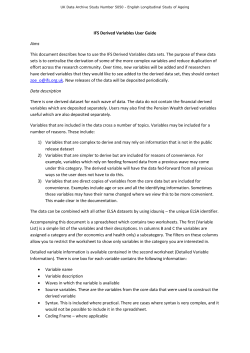
© Copyright 2026