1. education
2. school

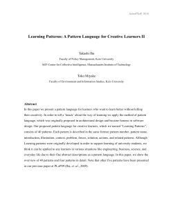
Lecture Notes for Numerical Methods, FEQA MSc
THE BUSINESS SCHOOL
FOR FINANCIAL MARKETS
Numerical Methods
FEQA MSc Lectures, Spring Term 2000
Data Modelling Module
Lecture 2
Implied Volatility
Professor Carol Alexander
Spring Term 2000
1
THE BUSINESS SCHOOL
FOR FINANCIAL MARKETS
1. What is Implied Volatility?
• Implied volatility is:
– the volatility of the underlying price process that is
'implicit' in the market price of the option, or put another
way:
– the forecast of the average volatility of the underlying over
the life of the option that is implicit in investors
expectations.
2
Prof. C.O. Alexander
Copyright ISMA centre, January 2000
Lecture Notes for Numerical Methods, FEQA MSc
THE BUSINESS SCHOOL
FOR FINANCIAL MARKETS
What Influences Implied Volatility?
• Implied volatility σ depends on:
– the price of the underlying S
– the market price of the option C
– the strike of the option K
– the maturity of the option t
– the interest rate r
– and any other variables that
influence the price of the option.
3
Prof. C.O. Alexander
THE BUSINESS SCHOOL
FOR FINANCIAL MARKETS
Black-Scholes Formula
If prices are governed by geometric
Brownian motion (GBM) and there is
perfect replication, then the current
price of a call option C has a closed
form analytic solution:
C = SN(x) - Ke-rtN(x-σ
σ√t)
where x measures the ‘moneyness’
of the option:
x = ln(S/Ke-rt) / σ√t + σ√t / 2
In-the-money (ITM)
x>0
At-the-money (ATM)
x=0
Out-of-the-money (OTM)
x<0
and N(x) is the normal distribution
function
Prof. C.O. Alexander
Copyright ISMA centre, January 2000
4
Lecture Notes for Numerical Methods, FEQA MSc
THE BUSINESS SCHOOL
FOR FINANCIAL MARKETS
Black-Scholes Implied Volatilities
• The values of S, K, r and t are all observable, so the
volatility which is ‘implied’ in an observed market price
C can be computed.
• No analytic form exists, but numerical methods
(described in Chriss pp330-340) are used to
approximate the value of the implicit function
σ = f( C, S, K, r, t)
• Usually volatility is quoted as an annualized percentage:
Volatility = 100 σ √250 %
5
Prof. C.O. Alexander
Example
THE BUSINESS SCHOOL
FOR FINANCIAL MARKETS
From the FT on June 15th ‘99: FTSE 100 Index options expiring on 18th June ‘99.
Strike
6250
6300
6350
6400
6450
6500
6550
6600
6650
6700
Price
223
176
132
92
58.5
33
16
5.5
2
0.5
Calls
vol
29.21
26.32
24.26
22.51
21.42
19.53
19.23
18.59
Volume
10
1
2
18
30
178
400
1966
0
1
Price
4
6.5
12.5
23
40
66.5
102.5
149
199
249
Puts
vol
23.65
21.55
20.4
19.28
17.9
16.57
14.48
14.05
-
The closing price on the FTSE was 6451.2.
Prof. C.O. Alexander
Copyright ISMA centre, January 2000
Volume
120
37
2
22
64
12
0
3
0
0
6
Lecture Notes for Numerical Methods, FEQA MSc
Call and Put Volatility Skews
THE BUSINESS SCHOOL
FOR FINANCIAL MARKETS
If call implied volatilities
are significantly
different from put
implied volatilities it is
because the evaluation
model is inadequate.
Figure 2.3a: Implied Volatilities on the FTSE 100 Index
Option, June 15th 1999
30
28
26
24
22
20
18
16
14
12
10
6200
6300
6400
6500
Calls
6600
Puts
6700
6800
Probably it is a model
based on spot price
whereas the hedging
instrument is a future.
7
Prof. C.O. Alexander
THE BUSINESS SCHOOL
FOR FINANCIAL MARKETS
Why the Differences between Call
and Put Implied Volatilities ?
• On June 15th 1999 the FTSE 100 future closed at 6486,
but its theoretical fair value was 6453.92
• So the market price of a call was based on 6486 but the
model price of the a call was based on 6453.92
• Market prices of call options therefore appear to be very
expensive and the only way that the model can account
for the high market price is to jack up the volatility.
• Similarly puts will appear less expensive than they
should, so the implied volatility that is backed out of the
model will be lower.
8
Prof. C.O. Alexander
Copyright ISMA centre, January 2000
Lecture Notes for Numerical Methods, FEQA MSc
THE BUSINESS SCHOOL
FOR FINANCIAL MARKETS
Differences between Implied and
Statistical Volatility
• Implied volatilities and
statistical volatilities are
both forecasting the same
thing: the volatility of the
underlying asset over the
life of the option.
• But the two types of
volatility measure often
differ.
• Because they use
different data and different
models:
30-day Volatility Forecasts
GBP-USD
25
20
15
10
5
0
May-88 May-89 May-90 May-91 May-92 May-93 May-94 May-95
GARCH30
EWMA
HIST30
IMP30
9
Prof. C.O. Alexander
THE BUSINESS SCHOOL
FOR FINANCIAL MARKETS
Differences between Implied and
Statistical Volatility
Implied volatility
Statistical volatility
Model is based on GBM:
Return distributions are:
dS/S = µ dt + σ dz
– price increments are
governed by a Wiener
process (so they are
independent and normal)
– the volatility σ of the
underlying asset S is
constant.
• Unconditional
– constant volatility
– weighted averages
• Conditional
– stochastic volatility
– GARCH or Diffusion
10
Prof. C.O. Alexander
Copyright ISMA centre, January 2000
Lecture Notes for Numerical Methods, FEQA MSc
THE BUSINESS SCHOOL
FOR FINANCIAL MARKETS
Differences between Implied and
Statistical Volatility
If statistical volatilities were correct, then differences
between the implied and statistical measures of volatility
would reflect a mis-pricing of the option. That is, the
wrong option model is being used, or investors have
irrational expectations.
If implied volatilities were correct (so the option
pricing model is an accurate representation of reality,
and investors expectations are correct so that there is
no over- or under- pricing in the options market), then
any observed differences between implied and
statistical volatilities would reflect inaccuracies in the
statistical forecast.
11
Prof. C.O. Alexander
THE BUSINESS SCHOOL
FOR FINANCIAL MARKETS
2. Smiles, Skews and
Volatility Term Structures
• The smile effect in implied volatility refers to the fact that
OTM options have higher implied volatilities than ATM
options.
• Thus the plot of implied volatility vs moneyness (or
strike) on a given day, for all options of a fixed maturity,
will be ‘smile’ shaped
Implied Volatility, σ
• The smile effect tends to
increase as the option
approaches expiry
0
Prof. C.O. Alexander
Copyright ISMA centre, January 2000
Moneyness, x
12
Lecture Notes for Numerical Methods, FEQA MSc
THE BUSINESS SCHOOL
FOR FINANCIAL MARKETS
Reasons for the Smile
• The volatility smile is a result of pricing model bias, and would
not be found if options were priced using an appropriate model.
• Black-Scholes is based on the assumption of GBM. But Volatility
is not constant, and neither are returns normally distributed.
• Thus OTM options have a greater chance of ending up ITM than
the Black-Scholes formula allows.
• Consequently the Black-Scholes formula is biased to underprice OTM options.
• This under-pricing of the model compared to observed market
behaviour yields higher implied volatilities for OTM options.
13
Prof. C.O. Alexander
THE BUSINESS SCHOOL
FOR FINANCIAL MARKETS
Reasons for the Skew
• The problem is compounded in equity markets because
they often exhibit a leverage effect.
• That is volatility is often higher following market falls
than it is following market rises of the same magnitude.
• So OTM puts require higher volatility to end up in-themoney than do OTM calls.
• This induces a pronounced negative ‘skew’ in the
volatility smile.
14
Prof. C.O. Alexander
Copyright ISMA centre, January 2000
Lecture Notes for Numerical Methods, FEQA MSc
Volatility Term Structures
THE BUSINESS SCHOOL
FOR FINANCIAL MARKETS
• On any fixed date a plot of the fixed-strike implied
volatilities of different maturities gives a term structure
of volatilities
• For example for the 6425 strike the implied volatility
term structure on 15th June 1999 looked something like
this:
25%
20%
months
15
Prof. C.O. Alexander
THE BUSINESS SCHOOL
FOR FINANCIAL MARKETS
Expiry end:
Strike
6275
6325
6375
6425
6475
6525
6575
6625
Call
Financial Times Prices of the FTSE 100
Index European Options on June 15th 1999
Jun
Put
169
126.5
89
57
33
16
6.5
2
11
19
31
49
75
108
148.5
194
Call
281
245
214
184
154.5
128.5
104
83
Jul
Put
101
115
133.5
154
174
197.5
223
252
Aug
Call Put
366.5
332.5
300
269.5
240
213
187
163.5
182
197.5
215
233.5
254
276
300
326
Sep
Put
Call
397
244
582.5
373
333
279
517.5
405.5
272
316.5 272
448
219
362
495.5
Call
219
Dec
Put
16
Prof. C.O. Alexander
Copyright ISMA centre, January 2000
Lecture Notes for Numerical Methods, FEQA MSc
THE BUSINESS SCHOOL
FOR FINANCIAL MARKETS
Behaviour of Volatility Term Structures
• Long term volatilities will change much less than short
term volatilities
• Volatility term structures mean revert to the long term
average
• They may slope upwards or downwards, although they
are not generally monotonic.
Current Market Conditions
Slope of Term Structure
Volatile
Downwards
Tranquil
Upwards
17
Prof. C.O. Alexander
THE BUSINESS SCHOOL
FOR FINANCIAL MARKETS
• A smile surface is a
surface plot of implied
volatilities for different
strikes (or moneyness)
and maturities
• Slicing through this surface
at a fixed strike or
moneyness gives a
volatility term structure
• Slicing through this surface
at a fixed maturity gives a
smile, which becomes
more pronounced as
maturity decreases
The Smile Surface
Figure 13: Smile surface of the FTSE, De 1
Implied Volatlity
1
0.8
0.6
0.4
0.2
0
-0.6
400
-0.4
-0.2
Moneyness
0
Prof. C.O. Alexander
Copyright ISMA centre, January 2000
200
0.2 0
Maturity
18
Lecture Notes for Numerical Methods, FEQA MSc
THE BUSINESS SCHOOL
FOR FINANCIAL MARKETS
Fitting Smile Surfaces
• Reliable market data for all strikes and maturities are
not available
• Data on OTM or very long term options is particularly
unreliable since quotes may be left unchanged for days
when trading is thin
• So smile surfaces must be interpolated using numerical
methods such as cubic splines (see Numerical recipes
in C).
19
Prof. C.O. Alexander
THE BUSINESS SCHOOL
FOR FINANCIAL MARKETS
Use of Smile Surfaces in
Dynamic Delta Hedging
• The most basic dynamic hedge is to match a position in
the underlying with an amount N(x) of an option
• This is hedge ratio is the option delta, and since
x = ln(S/Ke-rt) / σ√t + σ√t / 2
its value depends very much on implied volatility and
maturity, as predicted by the current smile surface
• As the underlying moves over time, the position will
need constant re-balancing to be delta neutral
• So, over a period of time, very large losses might be
made if the wrong hedging volatility is used
20
Prof. C.O. Alexander
Copyright ISMA centre, January 2000
Lecture Notes for Numerical Methods, FEQA MSc
3. Volatility Regimes
THE BUSINESS SCHOOL
FOR FINANCIAL MARKETS
6750
70.00
6500
60.00
6250
50.00
6000
40.00
5750
30.00
5500
5250
20.00
5000
10.00
Mar-99
Feb-99
Jan-99
Dec-98
Nov-98
Oct-98
Sep-98
Aug-98
Jul-98
Jun-98
Apr-98
May-98
Mar-98
Feb-98
4750
Jan-98
0.00
4500
4025
4075
4125
4175
4225
4275
4325
4375
4425
4475
4525
4575
4625
4675
4725
4775
4825
4875
4925
4975
5025
5075
5125
5175
5225
5275
5325
5375
5425
5475
5525
5575
5625
5675
5725
5775
5825
5875
5925
5975
6025
6075
6125
6175
6225
6275
6325
6375
6425
6475
6525
6575
6625
6675
6725
6775
6825
6875
6925
6975
ATM
FTSE100
How should we
model
movements in
implied
volatility smile
surfaces as the
underlying
price moves?
21
Prof. C.O. Alexander
THE BUSINESS SCHOOL
FOR FINANCIAL MARKETS
Derman’s ‘Sticky’ Models
1. Sticky Strike
2. Sticky Delta
3. Sticky Tree
Bounded Market
Trending Market
Jumpy Market
σK = σ0 - b(K-S0)
σK = σ0 - b(K-S)
σK = σ0 - b(K+S)
σK independent of S
σK increases with S
σK decreases with S
σATM = σ0 - b(S-S0)
σATM = σ0
σATM = σ0 - 2bS
σATM decreases as
price increases
σATM independent of
price
σATM moves twice as
fast as the skew
22
Prof. C.O. Alexander
Copyright ISMA centre, January 2000
Lecture Notes for Numerical Methods, FEQA MSc
Modelling the Relationship between
ATM Volatility and Price
THE BUSINESS SCHOOL
FOR FINANCIAL MARKETS
0.006
Probability
0.005
0.004
First question:
How is ATM
implied volatility
likely to move as
the underlying
price changes?
0.003
0.002
0.001
0
Change in
Equity Index
Change in ATM
Implied Volatility
23
Prof. C.O. Alexander
Scatter Plots
THE BUSINESS SCHOOL
FOR FINANCIAL MARKETS
Daily changes in FTSE and 1mth ATM vol
Daily changes in FTSE and 3mth ATM vol
10
10
8
8
6
6
4
4
2
2
0
-250
-200
-150
-100
-50
-2
0
0
50
100
150
200
250
-250
-200
-150
-100
-50
-2
-4
-4
-6
-6
-8
-8
-10
-10
0
50
100
150
200
24
Prof. C.O. Alexander
Copyright ISMA centre, January 2000
250
Lecture Notes for Numerical Methods, FEQA MSc
Scatter Plots
THE BUSINESS SCHOOL
FOR FINANCIAL MARKETS
Daily Change in Cable and 1M Imp Vol
Daily Change in Cable and 3M Imp Vol
3
8
2.5
6
2
1.5
4
1
0.5
2
-0.08
0
-0.08
-0.06
-0.04
-0.02
0
0.02
0.04
-0.06
-0.04
0
-0.02 -0.5 0
0.02
0.04
-1
0.06
-2
-1.5
-4
-2.5
-2
25
Prof. C.O. Alexander
THE BUSINESS SCHOOL
FOR FINANCIAL MARKETS
Constructing a Joint Distribution
of ∆S and ∆σATM
0.007
Probability
0.006
0.005
0.004
0.003
0.002
0.001
0
Change in
Implied Volatility
Change in Index
prob(∆σATM and ∆S) = prob(∆σATM∆S) prob(∆S)
26
Prof. C.O. Alexander
Copyright ISMA centre, January 2000
0.06
Lecture Notes for Numerical Methods, FEQA MSc
Estimating prob(∆σATM∆S)
THE BUSINESS SCHOOL
FOR FINANCIAL MARKETS
• To give conditional probabilities prob(∆σATM∆S) one
needs to model the relationship between implied
volatility and the price.
• The linear model of ATM implied volatility and the price
has been employed:
∆σATM = α + β ∆S + ε
in which case
∆σATM | ∆S ∼ N(α + β ∆S , σε2)
27
Prof. C.O. Alexander
Daily Data on σATM and S
THE BUSINESS SCHOOL
FOR FINANCIAL MARKETS
60
6500
55
6250
50
6000
45
5750
40
35
5500
30
5250
25
5000
20
4750
ATM
Mar-99
Mar-99
Jan-99
Feb-99
Jan-99
Feb-99
Dec-98
Dec-98
Nov-98
Oct-98
Oct-98
Nov-98
Oct-98
Sep-98
Sep-98
Aug-98
Jul-98
Jul-98
Aug-98
Jun-98
Jun-98
May-98
Apr-98
May-98
Apr-98
Mar-98
Mar-98
Jan-98
Feb-98
Feb-98
Jan-98
10
Jan-98
15
4500
Does the
FTSE100
index price
have a
negative
relationship
with 3
month ATM
volatility?
FTSE100
28
Prof. C.O. Alexander
Copyright ISMA centre, January 2000
Lecture Notes for Numerical Methods, FEQA MSc
Daily Data on σATM and S
THE BUSINESS SCHOOL
FOR FINANCIAL MARKETS
25
2.20
20
Does the
Cable rate
have a
negative
relationship
with 1
month ATM
volatility?
2.00
15
1.80
10
1.60
5
1M Imp Vol
Jul-95
Jul-94
Jan-95
Jul-93
Jan-94
Jan-93
Jul-92
Jul-91
Jan-92
Jan-91
Jul-90
Jul-89
Jan-90
Jan-89
Jul-88
1.40
Jan-88
0
Daily Clo.
29
Prof. C.O. Alexander
∆σATM = α + β ∆FTSE + ε
THE BUSINESS SCHOOL
FOR FINANCIAL MARKETS
Coefficient on Daily Change in FTSE
Significance of Coefficient on Daily Change in FTSE
0
0
-0.005
-2
-4
-0.01
-6
-0.015
-8
-0.02
-10
-0.025
Beta (1mth ATM)
Beta (2mth ATM)
Beta (3mth ATM)
tstat (1mthATM)
Jan-99
tstat (3mthATM)
30
Prof. C.O. Alexander
Copyright ISMA centre, January 2000
Feb-99
Mar-99
Dec-98
Oct-98
tstat (2mthATM)
Nov-98
Aug-98
Sep-98
Jun-98
Jul-98
Apr-98
May-98
Jan-98
Jan-99
Feb-99
Mar-99
Nov-98
Dec-98
Oct-98
Aug-98
Sep-98
Jun-98
Jul-98
-16
Apr-98
May-98
-0.035
Jan-98
Feb-98
Mar-98
-14
Feb-98
Mar-98
-12
-0.03
Lecture Notes for Numerical Methods, FEQA MSc
THE BUSINESS SCHOOL
FOR FINANCIAL MARKETS
Prob(∆S)
• We shall assume that prob(∆S) is represented by a
normal density
∆S ∼ N(µ, σ2)
• The parameters could be obtained from statistical
forecasts of the mean and variance.
• Their values will depend very much on current market
circumstances.
31
Prof. C.O. Alexander
THE BUSINESS SCHOOL
FOR FINANCIAL MARKETS
…on 31st March ‘99
• Assume the index was fairly stable, as reflected by a
marginal density for one-day changes in FTSE100 of
∆S ∼ N(0, 352).
• The OLS estimate of a linear relationship between the
one-day changes in 1 month ATM volatility ∆σATM and
∆S on 31.03.99 was:
∆σATM = -0.3 - 0.017 ∆S
(-2.73) (-10.01)
s.e. regression = 0.492
⇒ ∆σATM | ∆S ∼ N(−0.3 − 0.017 ∆S , 0.4922)
32
Prof. C.O. Alexander
Copyright ISMA centre, January 2000
Lecture Notes for Numerical Methods, FEQA MSc
THE BUSINESS SCHOOL
FOR FINANCIAL MARKETS
Prob(∆σATM and ∆S) in a Stable Market
FTSE100
31 Mar 99
0.01
Probability
0.009
0.008
0.007
0.006
0.005
0.004
0.003
0.002
0.001
0
Change in
Implied Volatility
Change in Index
∆S ∼ N(0, 352), ∆σATM | ∆S ∼ N(−0.3−0.017 ∆S , 0.4922)
33
Prof. C.O. Alexander
THE BUSINESS SCHOOL
FOR FINANCIAL MARKETS
Prob(∆σATM and ∆S) in a Jumpy Market
FTSE100
9th Oct 98
0.01
Probability
0.009
0.008
0.007
0.006
0.005
0.004
0.003
0.002
0.001
0
Change in
Implied Volatility
∆S ∼ N(−30, 602),
Change in Index
∆σATM | ∆S ∼ N(-0.03 ∆S, 1.252)
34
Prof. C.O. Alexander
Copyright ISMA centre, January 2000
Lecture Notes for Numerical Methods, FEQA MSc
4. Principal Component Models of
the Smile
THE BUSINESS SCHOOL
FOR FINANCIAL MARKETS
FTSE100 Index, 3 month ATM Volatility and the Skew: Jan ‘98 to Mar ‘99
60.00
6500
55.00
6250
50.00
6000
45.00
40.00
5750
35.00
5500
30.00
5250
25.00
5000
20.00
4750
Mar-99
Feb-99
Jan-99
Dec-98
Nov-98
Oct-98
Sep-98
Aug-98
Jul-98
Jun-98
May-98
Apr-98
Mar-98
Feb-98
10.00
Jan-98
15.00
4500
4025
4125
4225
4325
4425
4525
4625
4725
4825
4925
5025
5125
5225
5325
5425
5525
5625
5725
5825
5925
6025
6125
6225
6325
6425
6525
6625
6725
6825
6925
ATM
FTSE100
35
Prof. C.O. Alexander
Relationship between the Index and the
Skew Deviations
THE BUSINESS SCHOOL
FOR FINANCIAL MARKETS
Deviation of fixed strike volatility from ATM volatility
3 months
25.00
6500
20.00
6250
15.00
6000
10.00
5.00
5750
0.00
5500
-5.00
5250
-10.00
5000
-15.00
4750
Mar-99
Feb-99
Jan-99
Dec-98
Nov-98
Oct-98
Sep-98
Aug-98
Jul-98
Jun-98
May-98
Apr-98
Mar-98
Feb-98
-25.00
Jan-98
-20.00
4500
4025
4125
4225
4325
4425
4525
4625
4725
4825
4925
5025
5125
5225
5325
5425
5525
5625
5725
5825
5925
6025
6125
6225
6325
6425
6525
6625
6725
6825
6925
FTSE100
36
Prof. C.O. Alexander
Copyright ISMA centre, January 2000
Lecture Notes for Numerical Methods, FEQA MSc
Relationship between the Index and the
Skew Deviations
THE BUSINESS SCHOOL
FOR FINANCIAL MARKETS
1 month
40
6500
35
6250
30
25
6000
20
5750
15
10
5500
5
0
5250
-5
5000
-10
-15
4750
4500
Mar-99
Feb-99
Jan-99
Dec-98
Nov-98
Oct-98
Sep-98
Aug-98
Jul-98
Jun-98
May-98
Apr-98
Mar-98
Feb-98
-25
Jan-98
-20
4025
4075
4125
4175
4225
4275
4325
4375
4425
4475
4525
4575
4625
4675
4725
4775
4825
4875
4925
4975
5025
5075
5125
5175
5225
5275
5325
5375
5425
5475
5525
5575
5625
5675
5725
5775
5825
5875
5925
6025
6075
6125
6175
6225
6275
6325
6375
6725
37
6775
6425
6475
6525
6575
6625
6825
6875
6925
6975
FTSE100
Prof. C.O. Alexander
THE BUSINESS SCHOOL
FOR FINANCIAL MARKETS
6675
5975
Why Does σK - σATM Increase with S?
σK - σATM = -b (K - S)
1. Sticky Strike
2. Sticky Delta
3. Sticky Tree
Bounded Market
Trending Market
Jumpy Market
σK = σ0 - b(K-S0)
σK = σ0 - b(K-S)
σK = σ0 - b(K+S)
σK independent of S
σK increases with S
σK decreases with S
σATM = σ0 - b(S-S0)
σATM = σ0
σATM = σ0 - 2bS
σATM decreases as
index increases
σATM independent of
index
σATM moves twice as
fast as the skew
38
Prof. C.O. Alexander
Copyright ISMA centre, January 2000
Lecture Notes for Numerical Methods, FEQA MSc
THE BUSINESS SCHOOL
FOR FINANCIAL MARKETS
How Should the Skew be Modified as
the Index Changes?
• Step 1: Model the skew deviations from ATM volatility
with a principal component analysis on ∆(σK(t) - σATM(t)).
• Step 2: Model the relationship between the Index and
the skew deviations as:
ith principal component (t) = γ0,i (t) + γi (t) ∆FTSE + ηi (t)
[t = option maturity (1mth, 2mth or 3mth)]
39
Prof. C.O. Alexander
THE BUSINESS SCHOOL
FOR FINANCIAL MARKETS
PCA of the Skew Deviations
• A principal components analysis of the daily change in
σK - σATM shows that typically 80-90% of the variation in
σK - σATM can be explained by 3 principal components.
• The factor weights show that the principal components
are capturing:
– parallel shift (PC1)
– tilt (PC2)
– convexity (PC3)
40
Prof. C.O. Alexander
Copyright ISMA centre, January 2000
Lecture Notes for Numerical Methods, FEQA MSc
THE BUSINESS SCHOOL
FOR FINANCIAL MARKETS
Variation Explained by Principal
Components
3 month data
Eigenvalue
Cumulative R2
PC1
PC2
PC3
13.3574
2.257596
0.691317
0.742078
0.8675
0.905906
2 month data
Eigenvalue
Cumulative R2
PC1
PC2
PC3
19.68491
0.866442
0.834766
0.855866
0.893537
0.929831
1 month data
Eigenvalue
Cumulative R2
PC1
PC2
PC3
25.7177
11.6942
6.119627
0.476254
0.692813
0.806139
41
Prof. C.O. Alexander
THE BUSINESS SCHOOL
FOR FINANCIAL MARKETS
Strike
4225
4325
4425
4525
4625
4725
4825
4925
5025
5125
5225
5325
5425
5525
5625
5725
5825
5925
Factor Weights in PCA of σK - σATM
PC1
0.53906
0.6436
0.67858
0.8194
0.84751
0.86724
0.86634
0.80957
0.9408
0.92639
0.92764
0.93927
0.93046
0.90232
0.94478
0.94202
0.93583
0.90699
PC2
0.74624
0.7037
0.58105
0.48822
0.34675
0.1287
0.017412
-0.01649
-0.18548
-0.22766
-0.21065
-0.22396
-0.25167
-0.20613
-0.2214
-0.22928
-0.22818
-0.22788
PC3
0.26712
0.1862
0.035155
-0.03331
-0.19671
-0.41161
-0.43254
-0.28777
0.068028
0.13049
0.12154
0.14343
0.16246
0.017523
0.073863
0.073997
0.074602
0.068758
3 months
42
Prof. C.O. Alexander
Copyright ISMA centre, January 2000
Lecture Notes for Numerical Methods, FEQA MSc
ith PC = γ0,i + γi ∆FTSE + ηi
THE BUSINESS SCHOOL
FOR FINANCIAL MARKETS
30
γ1 (parallel shift) is
always positive and
usually very highly
significant.
25
20
15
10
5
0
-5
-10
tstat on pc1
tstat on pc2
Mar-99
Jan-99
Feb-99
Nov-98
Dec-98
Oct-98
Sep-98
Jul-98
Aug-98
Jun-98
Apr-98
May-98
γ3 (convexity) often has
the opposite sign to γ2.
Mar-98
Jan-98
-15
Feb-98
γ2 (tilt) is often negative
(stable market) but
sometimes positive (jumpy
market) or zero (trending
market).
tstat on pc3
43
Prof. C.O. Alexander
What Happens to σK - σATM as the
Index Increases in a Stable Market?
THE BUSINESS SCHOOL
FOR FINANCIAL MARKETS
σK - σATM
σK - σATM
γ1 > 0
γ2 < 0
+
K
(a) σK - σATM
increases with
the Index
σK - σATM
=
K
K
(b) The range (or
slope) of the skew
decreases as the
index increases
44
Prof. C.O. Alexander
Copyright ISMA centre, January 2000
Lecture Notes for Numerical Methods, FEQA MSc
Stable Market Regime
THE BUSINESS SCHOOL
FOR FINANCIAL MARKETS
Low K vol
Most of the
movement
in volatilities
comes from
the low
strikes
ATM vol
High K vol
S↑
As the index moves σK - σATM is relatively constant for low strike
volatilities
But for high strike volatilities σK - σATM decreases (increases) as
the index increases (decreases)
45
Prof. C.O. Alexander
What Happens to σK - σATM as the
Index Increases in a Jumpy Market?
THE BUSINESS SCHOOL
FOR FINANCIAL MARKETS
σK - σATM
σK - σATM
γ1 > 0
γ2 > 0
+
K
(a) σK - σATM
increases with
the Index
σK - σATM
=
K
K
(b) The range (or
slope) of the skew
increases as the
index increases
46
Prof. C.O. Alexander
Copyright ISMA centre, January 2000
Lecture Notes for Numerical Methods, FEQA MSc
Jumpy Market Regime
THE BUSINESS SCHOOL
FOR FINANCIAL MARKETS
Low K vol
Most of the
movement
in volatilities
comes from
the high
strikes
ATM vol
High K vol
S↑
As the index moves σK - σATM is quite stable for high strike
volatilities
But for low strike volatilities σK - σATM increases (decreases)
as the index increases (decreases)
47
Prof. C.O. Alexander
What Happens to σK - σATM as the
Index Increases in a Trending Market?
THE BUSINESS SCHOOL
FOR FINANCIAL MARKETS
σK - σATM
σK - σATM
γ1 > 0
γ2 = 0
+
K
(a) σK - σATM
increases with
the Index
σK - σATM
=
K
K
(b) The range of the
skew does not much
change as the index
increases
48
Prof. C.O. Alexander
Copyright ISMA centre, January 2000
Lecture Notes for Numerical Methods, FEQA MSc
Trending Market Regime
THE BUSINESS SCHOOL
FOR FINANCIAL MARKETS
Low K vol
There is not
so much
movement
in volatilities
at any strike
ATM vol
High K vol
S↑
As the index increases σK - σATM also increases for all strikes
So for some just OTM strikes σK - σATM can move from
negative to positive as the option moves to ITM
49
Prof. C.O. Alexander
Sticky Models vs PCA
THE BUSINESS SCHOOL
FOR FINANCIAL MARKETS
R-Squared from Linear Skew Parameterization
1.2
Sticky regimes
models assume the
skew is a linear
function of the strike
1
0.8
0.6
0.4
0.2
R-Sq 2m
Mar-99
Jan-99
Feb-99
Nov-98
Dec-98
Oct-98
Sep-98
Jul-98
R-Sq 1m
Aug-98
Jun-98
Apr-98
May-98
Mar-98
Jan-98
Feb-98
0
Principal component
analysis includes
linear and non-linear
effects
R-Sq 3m
50
Prof. C.O. Alexander
Copyright ISMA centre, January 2000
Lecture Notes for Numerical Methods, FEQA MSc
THE BUSINESS SCHOOL
FOR FINANCIAL MARKETS
Reading
N.A. Chriss (1997) Black-Scholes and Beyond IRWIN Chapter 8
E. Derman (1999) ‘Volatility Regimes’ RISK Magazine, April Issue
M. Kani and E. Derman (1997) ‘The Patterns of Changes in Implied
Index Volatilities’ Goldman Sachs Quantitative Strategies Research
Notes
M. Rubinstein (1994) ‘Implied Binomial Trees’ Jour. Finance 69, no. 3
pp 771-818
51
Prof. C.O. Alexander
Copyright ISMA centre, January 2000