OPERATIONALIZING THE USE OF LIDAR IN FOREST RESOURCE
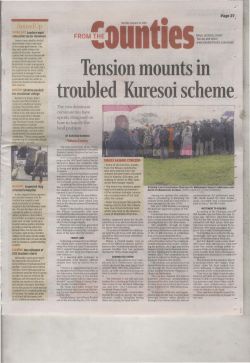
INVENTORIES: WHAT IS THE OPTIMAL POINT DENSITY?
Kevin Lim, Ph.D.
Lim Geomatics Inc.
264 Catamount Court, Ottawa, Ontario, K2M 0A9, Canada
[email protected]
Paul Treitz, Ph.D.
Queen’s University, Department of Geography
Kingston, Ontario, K2L 3N6, Canada
[email protected]
Murray Woods
Dave Nesbitt
Ontario Ministry of Natural Resources, Southern Science & Information Section
3301 Trout Lake Road, North Bay, Ontario, P1A 4L7, Canada
[email protected]
[email protected]
David Etheridge
Ontario Ministry of Natural Resources, Northern Science & Information Section
P.O. Bag 3020, South Porcupine, Ontario, P0N 1H0, Canada
[email protected]
ABSTRACT
Literature from the past two decades documents how airborne LIDAR can be used to predict forest inventory
variables, such as basal area, volume, and biomass, at the plot and stand level. However, a key question that has yet
to be fully addressed, and that the forest industry continues to ask as it considers operationalizing the use of LIDAR
in forest resource inventories, is: What is the optimal point density for predicting forest inventory variables? For
example, is a point density of 0.5 points/m2 sufficient for making accurate predictions of forest inventory variables
or is a point density of 3 points/m2 the minimum required? To investigate this key question, a three-year project was
launched in 2007 in Ontario, Canada. Field data for approximately 180 plots, sampling a broad range of forest types
and conditions in Ontario, were collected over two study sites. Airborne LIDAR data, characterized by 3 points/m2
were systematically decimated to produce datasets with point densities of approximately 1.5 and 0.5 points/m2.
Models, developed using stepwise regression, were developed for each of the three lidar datasets to estimate several
forest inventory variables including: (1) basal area (R2=0.25-0.94); (2) gross total volume (R2=0.46-0.95); (3) gross
merchantable volume (R2=0.37-0.94); (4) stem density(R2=0.23-0.89); (5) quadratic mean diameter (R2=0.59-0.86);
(6) total aboveground biomass (R2=0.26-0.93); (7) average height (R2=0.76-0.95); and (8) top height (R2=0.750.98). Aside from two cases, no decimation effect was found for predictions of forest variables, which suggests that
a point density of 0.5 points/m2 is sufficient for plot and stand level modelling under these forest conditions.
INTRODUCTION
Forest inventory and management requirements are changing rapidly as forest industries try to satisfy an
increasingly complex set of rules, standards, business practices, and public expectations (i.e., economic,
environmental and social policy goals). To satisfy these expectations, there is a critical need to develop accurate
inventory systems that spatially quantify forest structure and related attributes to enable product segregation and
resource value maximization (Pitt and Pineau, 2009). Over the past decade, research has clearly demonstrated the
capacity for light detection and ranging (LIDAR) and methodological approaches (i.e., derived LIDAR metrics and
models) to enhance our capacity for acquiring forest biophysical variables for forest planning and operations (Lim
and Treitz, 2004; Rooker Jensen et al. 2006; Gobakken and Næsset 2007; Bollandsås and Næsset 2007; Stephens et
ASPRS 2010 Annual Conference
San Diego, California April 26-30, 2010
al. 2007; Thomas et al., 2008; Woods et al., 2008). These technologies and methods are now starting to be
implemented operationally in forests around the world (Næsset 2004; Holmgren and Jonsson 2004). However,
standards for the acquisition, processing, and application of LIDAR data for forestry and natural resources inventory
and management do not currently exist. For example, data acquisition standards (e.g., sampling density) that
determine the optimal acquisition of LIDAR data for forestry (in terms of forest variable estimation and cost
efficiency) have yet to be developed. These standards are required if the forest industry is to gain the best possible
return from the technology across a range of forest conditions and for specific operational requirements. The goal of
this research is to identify standards for collecting, processing and analysing LIDAR data to derive forest inventory
attributes that lead to the production of an enhanced forest resource inventory (eFRI) for Ontario forests. Here, we
report on the impact of LIDAR point density on the prediction of forest inventory variables.
STUDY AREAS
Two study areas, Swan Lake Research Reserve (SLRR) and the Romeo Malette Forest (RMF) provided a
range of forest species common to central and northern Ontario (Figure 1).
Swan Lake Research Reserve
Figure 1. The geographic location of the Swan Lake Research Reserve
and Romeo Malette Forest in Ontario, Canada.
The SLRR is located 250 km
north of Toronto and east of
Huntsville, Ontario, within Algonquin
Provincial Park. The 2,000 hectares
(ha) site situated in Peck Township is
located at 45° 28' N, 78° 45' W and
ranges in elevation from 410 to 590 m
above sea level (asl). This site lies on
the Precambrian Shield and is
characterized by rolling hills and high
rocky ridges that are separated by
valleys scoured by glaciation.
Outwash flats, ablation moraines, and
drumlinoid deposits provide soil
deposits ranging from coarse to
medium texture. The Algonquin
Dome, due to its elevation, has a
climate that is generally more cool and
wet than its surrounding areas (Cole
and Mallory 2005).
The site is within the Great
Lakes–St. Lawrence Forest region and
comprises mature stands of shade– and
mid–tolerant hardwoods (sugar maple
[Acer saccharum Marsh.], American
beech [Fagus grandifolia Ehrh.], soft
maple [Acer rubrum L.], yellow birch
[Betula
alleghaniensis
Britt.],
ironwood [Ostrya virginiana (Mill.)
K. Koch]), conifers (eastern hemlock
[Tsuga canadensis (L.) Carrière],
white pine [Pinus strobus L.], white
spruce [Picea glauca (Moench) Voss],
red spruce [Picea rubens Sarg.],
eastern
larch
[Larix
laricina (Du ROI) K. Koch], eastern
ASPRS 2010 Annual Conference
San Diego, California April 26-30, 2010
white cedar [Thuja occidentalis L.], balsam fir [Abies balsamea (L.) Mill.]), and minor proportions of mid–tolerant
and intolerant hardwoods (i.e., white birch [Betula papyrifera Marsh.], black cherry [Prunus serotina Ehrh.], white
ash [Fraxinus americana L.], black ash [Fraxinus nigra Marsh.], and trembling aspen [Populus tremuloides
Michx.]).
Romeo Malette Forest
The RMF is located in the northeast portion of Ontario’s Boreal Forest near Timmins, Ontario. The RMF is an
active forest management unit with approximately 532,000 productive forest hectares. The forest is characterized by
extensive coniferous stands on poorly drained lowlands and gently rising uplands. The northern portion (40% of the
forest area) located on clay is best described as relatively flat to gently rolling, interspersed with depressions and
eskers. The elevation ranges from 305 to 320 metres above sea level with extensive clay deposits, high water table
and poor drainage. The remaining southern area of the forest consist mainly of glacial deposits of bouldery sand till
overlying bedrock with elevation ranges from 305 to 380 metres asl with moderately rolling topography with
generally good drainage. The dominant species are black spruce [Picea mariana (Mill) B.S.P.], white birch,
trembling aspen, jack pine [Pinus banksiana Lamb.], eastern white cedar, white spruce, eastern larch, and balsam fir.
Other minor species include black ash, yellow birch, soft maple and red [Pinus resinosa Ait.] and white pine.
The RMF has a relatively cool climate with a mean annual temperature of 1.4°C. Temperature ranges from an
extreme low of –45 °C to an extreme high of 35 °C. The growing season (period when mean temperature is above
5.6°C) is approximately 160 days. The average annual precipitation is 77.5 cm with 50.8 cm falling as rain, the
balance as snow. Average annual snowfall is 275.8 cm and summer rainfall (May to September) is approximately
37.6cm.
METHODS
Field Data
Ground reference data were collected for the two study areas during the period of November to December
2007 and May to October 2008. A circular fixed area plot of 400 m2 was established for sampling all forest types
except for the tolerant hardwood group where a 1000 m2 plot size was used to better represent metrics of unevenaged size class structures. Forest types sampled were: (i) tolerant hardwoods (sugar maple, beech, and yellow birch);
(ii) black spruce; (iii) jack pine; (iv) intolerant hardwoods (white birch and trembling aspen); and (v) mixedwoods.
For each plot, all trees larger than or equal to 9.1 cm diameter at breast height (DBH) were measured with a
diameter tape. Each tree was assessed for species, status (live or dead), crown class (dominant, co–dominant, etc.)
and visual quality. A Vertex™ hypsometer was used to measure height to base of live crown and total tree height for
every tree. Heights of deciduous species were measured in a leaf–off period to obtain the most accurate height
possible. The centre of each circular plot was geo–referenced with a Trimble Pro XT™ kinematic GPS unit
connected to a Hurricane™ antenna, which was mounted on a tripod. A minimum of 300 points were collected for
each post position and later post–processed against a base station to achieve sub–meter accuracy. Plot data
consisting of individual tree data were compiled to per ha values using the equations presented in Table 1.
Summary plot statistics, including top height (TOPHT), average height (AVGHT), basal area (SUMBA),
density (DENSITY), quadratic mean DBH (QMDBH), gross total volume (SUMGTV), gross merchantable volume
(SUMGMV), and aboveground biomass (BIOMASS), are presented in Table 2 by study site and forest or species
grouping if applicable.
LIDAR Data and Data Processing
LIDAR data were collected in August 2007 using an Optech ALTM3100 airborne laser scanner mounted in a
Cessna 208B Grand Caravan. The base mission was flown at 1000 m with a scan rate of 54 Hz and a maximum
pulse repetition frequency of 100,000 Hz. This configuration resulted in a cross track spacing of 0.50 m, an along
track spacing of 0.57 m, an average sampling density of 3.2 points/m2, and a swath width of approximately 475 m.
The LIDAR point cloud data were classified as ground or vegetation by the vendor using proprietary algorithms. A
bald-earth DEM was derived from the classified ground returns. All LIDAR point data were normalized to the
terrain (i.e., given a return and its x-y coordinate, subtract the z-value for that x-y coordinate on the DEM from its
original z-value).
ASPRS 2010 Annual Conference
San Diego, California April 26-30, 2010
Table 1. Equation or method used to calculate forest variables
Ground Metric
Top Height (m)
Average Height (m)
Density (stems ha-1)
Quadratic Mean DBH (cm)
2
Description
Calculated as the average of the largest 100 stems per hectare.
Calculated as the average height of all trees 9.1 cm and larger.
Number of live trees 9.1 cm and larger expressed per hectare.
∑
-1
Basal Area (m ha )
Gross Total Volume (m3 ha-1)
(Honer et al. 1983)
Gross Merchantable Volume (m3 ha-1)
(Honer et al. 1983)
⎡(
DBH 2 n )⎤ where n is stems per plot.
⎢⎣
⎥⎦
2
DBH * .00007854
Per hectare value calculated by summing each tree per plot.
= ß1 * DBH2*(1-0.04365* ß2)2/( ß3+(0.3048 * ß4/Ht))
Individual tree volume equation.
Coefficients vary by species.
Per hectare value calculated by summing each tree per plot.
= SUMGTV * (ß1 + ß2(X) + ß3(X))
X = [(1+hs/ht)(Dtop2/DBH2)]
HS = Stump Height
HT = Total Height
Dtop = Minimum Top Diameter
MV = Merchantable Volume
Aboveground Biomass (Kg ha-1)
(Ter-Mikaelian and Korzukhin, 1997)
Individual tree volume equation.
Coefficients varies by species.
Per hectare value calculated by summing each tree per plot.
= ß1 * Dbhß2
Individual tree above ground biomass equation.
Coefficients vary by species.
Per hectare value calculated by summing each tree per plot.
Table 2. Summary plot statistics for the SLRR and PRF
Variable
TOPHT (m)
AVGHT (m)
SUMBA (m2/ha)
DENSITY (stems/ha)
QMDBH (cm)
SUMGTV (m3/ha)
SUMGMV (m3/ha)
BIOMASS (Kg/ha)
Variable
TOPHT (m)
AVGHT (m)
SUMBA (m2/ha)
DENSITY (stems/ha)
QMDBH (cm)
SUMGTV (m3/ha)
SUMGMV (m3/ha)
BIOMASS (Kg/ha)
SLRR
RMF
Tolerant Hardwood (N=32)
Intolerant Hardwoods (N=33)
Mean
Mean
Mean
Mean
Mean
Min.
Max.
Std. Dev.
24.9
22.6
22.6
22.6
22.6
17.3
35.8
5.4
18.9
16.7
16.7
16.7
16.7
11.7
32,9
5.3
25.9
31.4
31.4
31.4
31.4
13.5
58.8
13.8
421.0
1198.5
1198.5
1198.5
1198.5
75.0
1826.2
393.8
28.5
18.2
18.2
18.2
18.2
13.89
55.3
10.4
232.8
266.5
266.5
266.5
266.5
106.9
770.9
209.3
201.9
216.2
216.2
216.2
216.2
75.5
742.9
206.7
203514 128732 128732
128732
128732
60853
246965
56780
RMF
Jack Pine (N=35)
Black Spruce (N=34)
Mean
Mean
Mean
Mean
Mean
Min.
Max.
Std. Dev.
20.2
16.7
16.7
16.7
16.7
11.7
24.8
3.1
16.1
12.9
12.9
12.9
12.9
8.9
19.8
2.1
21.2
25.8
25.8
25.8
25.8
12.9
53.9
9.6
1414.5
1643.0
1643.0
1643.0
1643.0
600.4
2376.6
470.5
17.0
14.2
14.2
14.2
14.2
12.2
22.7
2.8
248.8
162.7
162.7
162.7
162.7
57.7
464.0
94.1
105.4
109.0
109.0
109.0
109.0
28.3
401.1
88.7
127458 100833 100833
100833
100833
43966
244507
45404
ASPRS 2010 Annual Conference
San Diego, California April 26-30, 2010
The LIDAR data were decimated according to the methodology described by Raber et al. (2007). Decimation
level 0 (D0) represents the original dataset characterized by a point density of approximately 3 points/m2. The
decimation level 1 (D1) LIDAR dataset was derived by taking alternating points along each scan line with each scan
line retained, thereby increasing the cross track spacing by a factor of two. For the decimation level 2 (D2) LIDAR
dataset, every fourth point along each scan line was retained, thereby increasing the cross track spacing by a factor
of 4, and every other scan line was retained, resulting in an increase in the along track spacing by a factor of 2. The
systematic decimation resulted in the D1 and D2 LIDAR datasets possessing point densities of approximately 1.5
and 0.5 points/m2, respectively.
LIDAR Canopy Height and Density Predictors
Three types of predictors (i.e., statistical, canopy height, and canopy density) were derived from the
normalized LIDAR data. No height thresholds were used to filter any of the point data. The statistical group of
predictors included mean height and standard deviation (stddev) of LIDAR height measurements. The canopy height
predictors consisted of deciles of LIDAR canopy height (i.e., p10…p90) and the maximum (max) LIDAR height.
For each plot the range of LIDAR height measurements was divided into 10 equal intervals and the cumulative
proportion of LIDAR returns found in each interval, starting from the lowest interval (i.e., d1), was calculated. Since
the last interval always sums to a cumulative probability of 1, it was excluded resulting in 9 canopy density metrics
(i.e., d1 … d9). The remaining two canopy density metrics were calculated as the number of first returns divided by
all returns intersecting a sample plot (Da) and the number of first and only returns divided by all returns intersecting
a sample plot (Db).
Statistical Analyses
Stepwise regression and a significance level of 0.05 were used for model building. A diagnosis of each model
was performed to determine if parametric statistical assumptions were satisfied. The Shapiro-Wilk Test was used to
determine if residuals were normally distributed, whereas the Brown-Forsythe Test was used to check for the
presence of heteroschedasticity (i.e., unequal error variance).
As LIDAR predictors have been reported to be highly correlated, the variance inflation factors (VIF) for the
predictors used in a model were examined (Neter et al., 1996). Candidate models where predictors exhibited VIF
greater than 10 were discarded, as values above 10 suggest the presence of multi-collinearity in the predictor data
(Neter et al., 1996).
Repeated measures ANOVA was used to investigate the effect of decimation on predictions of forest variables.
A repeated measures ANOVA is used when all members of a sample are measured repeatedly under a number of
different conditions. Within the context of this study, it was a particular forest variable for a plot that was repeatedly
predicted using LIDAR data of three varying point densities. Given repeated measurements, the use of a standard
ANOVA is not appropriate (Popescu and Zhao, 2008). The hypothesis tested with repeated measures ANOVA was:
Does point density (i.e., 3, 1.5 and 0.5 points/m2) influence predictions of each of the forest variables considered in
this study? This is referred to as a within-subjects test.
RESULTS
Swan Lake Research Reserve – Tolerant Hardwoods
The regression models at each decimation level by forest variable for the SLRR are reported in Table 3. An
assessment of the percent root mean square error (RMSE) for each forest variable by decimation level shows little
variability. With the exception of QMDBH, no decimation effect was found for any of the other forest variables
considered for the SLRR (i.e., with the exception of QMDBH, Wilk’s Lamda p values were greater than 0.195 for
the other forest variables) (Table 4). For QMDBH at D0, the R2 was 0.592 compared a R2 of 0.702 and 0.703 for D1
and D2, respectively. This indicates that the model for the D0 dataset (high density) is accounting for less of the
variability in the observations in comparison to the models derived for the D1 and D2 datasets (lower densities).
ASPRS 2010 Annual Conference
San Diego, California April 26-30, 2010
Table 3. Models developed for each decimation level by forest variable for SLRR – Tolerant Hardwoods
Variable
SUMBA
(m2/ha)
SUMGTV
(m3/ha)
SUMGMV
(m3/ha)
DENSITY
(stems/ha)
QMDBH
(cm)
AVGHT
(m)
TOPHT
(m)
SUMBIO
(kg/ha)
Dec.
Level
D0
D1
D2
D0
D1
D2
D0
D1
D2
D0
D1
D2
D0
D1
D2
D0
D1
D2
D0
D1
D2
D0
D1
D2
R2
Equation
34.8 - 16.7 d7
35.2 - 17.4 d7
34.3 - 16.0 d7
84.8 + 7.63 p50 + 6.58 p10
198 - 201 d7 + 6.65 p10 + 4.69 Da
93.6 + 7.30 p10 + 7.08 p50
27.6 + 10.3 p50
28.4 + 10.3 p50
67.5 + 6.99 p50 + 6.07 p10
1518 - 111 stddev - 12.3 p10 - 10.9 Da
464 + 794 d8 + 27.8 p20 - 34.1 max
617 + 673 d8 + 26.3 p20 - 35.9 max
6.33 + 2.26 stddev - 17.2 d7 + 0.600 Da
27.8 - 27.1 d8 + 64.6 d2 + 0.876 p10 + 0.331 Da
50.5 - 20.5 d8 + 62.0 d2 + 1.04 p10 - 0.281 Db
9.97 + 0.738 p50 - 0.0987 Db + 4.29 d8
10.1 + 0.746 p50 - 0.105 Db + 4.53 d8
- 0.43 + 0.744 p50 + 0.132 Da + 4.50 d8
6.44 + 0.889 p80
6.64 + 0.879 p80
6.97 + 0.865 p80
208918 - 194385 d7 + 3821 Da
287254 - 156798 d7
182026 + 7783 p10
0.262
0.277
0.245
0.458
0.558
0.469
0.375
0.374
0.456
0.761
0.842
0.830
0.592
0.702
0.703
0.837
0.836
0.850
0.764
0.758
0.751
0.360
0.279
0.257
R2
(Adj.)
0.237
0.253
0.220
0.420
0.511
0.433
0.354
0.353
0.418
0.736
0.825
0.812
0.548
0.658
0.660
0.820
0.819
0.834
0.756
0.749
0.743
0.315
0.255
0.232
RMSE
3.17
3.14
3.20
29.18
26.34
28.86
28.93
28.94
26.98
51.85
42.14
43.73
2.31
1.97
1.97
0.62
0.62
0.59
0.83
0.84
0.86
26,884
28,532
28,966
RMSE
(%)
12.64
12.50
12.78
12.92
11.66
12.78
14.77
14.78
13.78
12.70
10.32
10.71
8.37
7.15
7.13
3.36
3.37
3.23
3.45
3.50
3.55
13.62
14.46
14.68
Table 4. Results from repeated measures ANOVA for the Tolerant Hardwoods
Variable
SUMBA
SUMGTV
SUMGMV
DENSITY
QMDBH
AVGHT
TOPHT
SUMBIO
Decimation Effect?
No
No
No
No
Yes
No
No
No
Value
0.893
0.894
0.927
0.944
0.595
0.991
0.910
0.935
MANOVA – Wilk’s Lamda
F
1.73
1.71
1.14
0.87
9.85
0.14
1.43
1.01
p
0.195
0.199
0.334
0.431
0.001
0.872
0.256
0.376
Romeo Malette Forest
Intolerant Hardwoods. The regression models at each decimation level by forest variable for the intolerant
hardwood forest grouping are reported in Table 5. It is interesting to note that in most instances, the same LIDAR
predictors are selected during stepwise regression model building and again exhibit limited variability in percent
RMSE. The repeated measures ANOVA results (Table 6) did not identify a decimation effect for any of the forest
variables in the intolerant forest grouping (Wilk’s Lamda p values > 0.32) for the RMF.
Jack Pine. The regression models at each decimation level by forest variable for the jack pine forest grouping
are reported in Table 7. Similar to results reported for other sites and groupings, with the exception of DENSITY,
the percent RMSE values for each variable by decimation level are very similar to each other. Excluding DENSITY,
no decimation effect was found for any of the other forest variables in the jack pine forest grouping (i.e., Wilk’s
Lamda p values were greater than 0.37 for the other forest variables) (Table 8).
ASPRS 2010 Annual Conference
San Diego, California April 26-30, 2010
Black Spruce. The regression models at each decimation level by forest variable for the black spruce forest
grouping are reported in Table 9. The repeated measures ANOVA results (Table 10) did not identify a decimation
effect for any of the forest variables in the black spruce forest grouping (Wilk’s Lamda p values > 0.259) in the
RMF.
Table 5. Models developed for each decimation level by forest variable for RMF-Intolerant Hardwoods
Variable
SUMBA
(m2/ha)
SUMGTV
(m3/ha)
SUMGMV
(m3/ha)
DENSITY
(stems/ha)
QMDBH
(cm)
AVGHT
(m)
TOPHT
(m)
SUMBIO
(kg/ha)
Dec.
Level
D0
D1
D2
D0
D1
D2
D0
D1
D2
D0
D1
D2
D0
D1
D2
D0
D1
D2
D0
D1
D2
D0
D1
D2
R2
Equation
- 16.1 + 4.16 mean
- 16.1 + 4.15 mean
- 15.8 + 4.12 mean
- 175 + 30.0 p80 - 331 d2
- 261 + 45.6 p80 - 38.9 stddev
- 267 + 30.7 p80
- 310 + 30.3 p80
- 312 + 30.3 p80
- 308 + 30.1 p80
1875 - 2465 d3
1853 - 2413 d3
1867 - 2486 d3
1.06 + 0.925 p90
1.05 + 0.925 p90
0.93 + 0.932 p90
8.01 + 0.498 p80
7.99 + 0.499 p80
8.03 + 0.496 p80
3.04 + 0.628 p90 + 0.356 max
3.03 + 0.627 p90 + 0.359 max
3.29 + 0.629 p90 + 0.351 max
- 103147 + 20390 mean
- 103157 + 20351 mean
- 101819 + 20193 mean
0.837
0.833
0.823
0.880
0.877
0.860
0.873
0.871
0.877
0.239
0.227
0.248
0.842
0.843
0.840
0.767
0.764
0.773
0.941
0.939
0.943
0.788
0.784
0.775
R2
(Adj.)
0.831
0.827
0.817
0.872
0.868
0.855
0.869
0.867
0.873
0.214
0.201
0.223
0.837
0.838
0.834
0.75
0.756
0.766
0.937
0.935
0.939
0.781
0.777
0.767
RMSE
4.45
4.50
4.62
42.17
42.70
45.52
42.14
42.55
41.56
272.68
274.84
271.06
1.50
1.50
1.51
1.00
1.01
0.99
0.89
0.90
0.87
25,562
25,789
26,332
RMSE
(%)
14.12
14.29
14.68
15.76
15.96
17.01
19.40
19.59
19.13
22.78
22.96
22.65
8.21
8.20
8.28
6.02
6.05
5.93
3.95
4.01
3.87
19.68
19.85
20.27
Table 6. Results from repeated measures ANOVA for the intolerant hardwoods forest type grouping
Variable
SUMBA
SUMGTV
SUMGMV
DENSITY
QMDBH
AVGHT
TOPHT
SUMBIO
Decimation Effect?
No
No
No
No
No
No
No
No
Value
0.972
0.986
0.975
0.978
0.995
0.924
0.993
0.972
MANOVA – Wilk’s Lamda
F
0.42
0.21
0.37
0.32
0.08
1.19
0.10
0.41
ASPRS 2010 Annual Conference
San Diego, California April 26-30, 2010
p
0.660
0.813
0.696
0.727
0.927
0.320
0.908
0.666
Table 7. Models developed for each decimation level by forest variable for RMF-Jack Pine
Variable
SUMBA
(m2/ha)
Dec.
Level
D0
D1
D2
D0
D1
D2
D0
D1
D2
R2
Equation
R2
(Adj.)
0.784
0.770
0.792
0.884
0.878
0.880
0.847
0.865
0.899
RMSE
RMSE
(%)
13.73
14.39
13.48
12.50
12.80
12.71
17.21
15.91
13.35
5.82 + 2.10 p60 - 28.4 p10 + 0.842 p40
0.803
4.29
0.17 + 4.21 mean - 5.94 p20
0.783
4.49
5.16 + 2.94 mean - 7.17 p20 + 1.07 p40
0.810
4.21
SUMGTV
- 79.1 + 44.1 mean - 57.0 p20
0.891
31.11
(m3/ha)
- 74.1 + 43.2 mean - 51.3 p20
0.886
31.84
- 74.6 + 43.9 mean - 52.6 p20
0.887
31.64
SUMGMV
- 156 + 20.4 p90 + 6.10 p40
0.856
33.63
(m3/ha)
- 69.5 + 20.9 p90 + 6.96 p40 - 3.14 Da
0.877
31.09
- 3.7 + 15.4 p90 + 8.05 p40 - 37.7 p20 - 4.98 Da +
0.913
26.08
7.95 p60
DENSITY D0
659 + 57.4 Da - 1604 p10 - 75.0 max + 96.4 p40
0.650
0.604
278.19
19.67
(stems/ha) D1
- 867 + 72.1 Da
0.372
0.353
372.74
26.35
D2
- 475 + 61.1 Da
0.298
0.276
394.28
27.87
QMDBH
D0
- 8.17 + 0.805 max + 0.152 Db
0.713
0.695
1.48
8.66
(cm)
D1
9.24 + 0.703 max - 0.179 Da
0.732
0.715
1.43
8.37
D2
3.99 + 0.701 max
0.671
0.661
1.58
9.27
AVGHT
D0
12.9 + 0.471 p70 + 7.88 d2 - 9.31 d6
0.866
0.853
0.79
4.89
(m)
D1
16.1 + 0.432 p70 - 10.7 d7 + 6.10 d2
0.857
0.844
0.81
5.05
D2
10.3 + 0.525 p70 + 8.64 d2 - 7.87 d5
0.849
0.835
0.83
5.19
TOPHT
D0*
14.3 - 0.182 p40 + 0.901 max - 6.66 d4 - 8.34 d8
0.981
0.979
0.42
2.08
(m)
D1
3.91 + 0.557 p90 + 0.399 max
0.974
0.972
0.50
2.46
D2
4.71 + 0.633 p90 + 0.305 max
0.967
0.965
0.56
2.75
SUMBIO
D0
- 178881 + 24006 mean - 33568 p20 + 2033 Db
0.852
0.837
17,479
13.71
(kg/ha)
D1
28639 + 21390 mean - 27034 p20 - 1902 Da
0.843
0.828
17.972
14.10
D2
- 160390 + 24132 mean - 30628 p20 + 1745 Db
0.846
0.831
17,842
14.00
* Model developed using best subsets regression as regression modelling assumptions could not be met based on
models developed using stepwise regression despite dependent and independent variable transformations.
Table 8. Results from repeated measures ANOVA for the jack pine forest type grouping
Variable
SUMBA
SUMGTV
SUMGMV
DENSITY
QMDBH
AVGHT
TOPHT
SUMBIO
Decimation Effect?
No
No
No
Yes
No
No
No
No
Value
0.980
0.992
0.951
0.646
0.940
0.982
0.993
0.993
MANOVA – Wilk’s Lamda
F
0.33
0.12
0.82
8.78
1.03
0.30
0.10
0.12
ASPRS 2010 Annual Conference
San Diego, California April 26-30, 2010
p
0.721
0.885
0.448
0.001
0.370
0.746
0.908
0.888
Table 9. Models developed for each decimation level by forest variable for RMF-Black Spruce
Variable
SUMBA
(m2/ha)
SUMGTV
(m3/ha)
SUMGMV
(m3/ha)
DENSITY
(stems/ha)
QMDBH
(cm)
AVGHT
(m)
TOPHT
(m)
SUMBIO
(kg/ha)
Dec.
Level
D0
D1
D2
D0
D1
D2
D0
D1
D2
D0
D1
D2
D0
D1
D2
D0
D1
D2
D0
D1
D2
D0
D1
D2
R2
Equation
58.9 - 20.2 d5 + 1.58 p50 - 0.379 Db
- 0.91 + 2.23 p50 + 0.622 Da
48.6 + 1.26 p60 + 1.27 p40 - 0.478 Db
- 702 + 32.1 mean - 210 d6 + 873 d9 - 110 p20
- 66.3 + 42.2 mean - 5.59 p30
268 + 23.5 mean - 3.30 Db + 4.95 p40
- 114 + 5.63 p40 + 17.4 p90
- 182 + 20.1 p80 + 7.02 p40 + 113 d4
- 195 + 41.5 mean + 164 d3 - 282 p10
- 112 - 4076 d3 + 3254 p10 - 159 p30 - 180 p80 56.4 Db + 106 p40 + 9705 d9
5380 - 4678 d4 + 5580 p10 - 134 p30 - 95.9 p90
11212 - 2363 d4 - 204 p90 - 80.4 Db + 70.5 p40
8.03 + 1.18 p90 - 0.327 Da - 0.138 p40
8.58 + 1.07 p90 - 0.308 Da
2.44 + 1.12 p90 - 0.234 Da + 5.33 d6
2.41 + 0.948 p90 + 2.80 d1 - 0.0821 Da
1.73 + 0.836 p90 + 2.99 d2
2.34 + 0.802 p90 + 2.26 d3
2.32 + 0.547 max + 0.436 p90
2.10 + 0.578 max + 0.429 p90
3.79 + 0.577 max + 0.326 p90
- 321894 + 15682 mean - 114298 d6 + 427669 d9
- 17265 + 21243 mean
157912 + 11931 mean - 1752 Db + 3131 p40
RMSE
0.918
0.910
0.935
0.949
0.927
0.942
0.916
0.915
0.939
0.888
R2
(Adj.)
0.909
0.904
0.929
0.942
0.922
0.936
0.910
0.907
0.933
0.857
3.01
3.15
2.66
17.96
21.52
19.14
18.19
18.25
15.46
231.84
RMSE
(%)
11.68
12.22
10.33
11.04
13.23
11.77
16.69
16.74
14.18
14.11
0.794
0.861
0.838
0.783
0.863
0.951
0.941
0.936
0.923
0.927
0.903
0.925
0.905
0.932
0.766
0.842
0.822
0.769
0.850
0.946
0.938
0.932
0.918
0.922
0.897
0.918
0.902
0.925
313.83
257.74
0.82
0.95
0.76
0.49
0.53
0.56
0.69
0.66
0.77
11,673
13,199
11,143
19.10
15.69
5.80
6.72
5.34
3.81
4.16
4.34
4.10
3.98
4.58
11.58
13.09
11.05
Table 10. Results from repeated measures ANOVA for the black spruce forest type grouping
Variable
SUMBA
SUMGTV
SUMGMV
DENSITY
QMDBH
AVGHT
TOPHT
SUMBIO
Decimation Effect?
No
No
No
No
No
No
No
No
Value
0.984
0.983
0.985
0.935
0.916
0.982
0.987
0.970
MANOVA – Wilk’s Lamda
F
0.25
0.27
0.23
1.08
1.41
0.29
0.21
0.48
p
0.784
0.767
0.795
0.354
0.259
0.752
0.811
0.624
DISCUSSION AND CONCLUSION
With the exception of two cases, specifically QMDBH for SLRR and DENSITY for the jack pine grouping in
RMF, predictions of forest variables were not influenced by decimation level. Comparisons between R2, RMSE and
percent RMSE show little deviation for the forest variables considered. The results indicating a decimation effect for
DENSITY is not surprising since this forest variable is often the most difficult to predict using LIDAR data. In the
case of QMDBH, further investigation is required for this deviation since this variable is most often predicted quite
well from LIDAR data as illustrated by the other reported results in this study and others (e.g., Woods et al., 2008).
ASPRS 2010 Annual Conference
San Diego, California April 26-30, 2010
The results reported are promising and suggest that a point density of 0.5/m2 is sufficient for predicting forest
variables at the plot and stand level and that the assumption that higher sampling point densities lead to better
predictions needs to be challenged.
ACKNOWLEDGEMENTS
The authors wish to express their gratitude to Dr. Doug Pitt of the Canadian Wood Fibre Centre and the
Ontario Centre of Excellence for Earth and Environmental Technologies for their financial support of this
investigation. Special thanks to the many field crews for their competent work under seasonal conditions.
REFERENCES
Bollandsås, O.M., and E., Næsset, 2007. Estimating percentile-based diameter distributions in uneven-sized Norway
spruce stands using airborne laser scanner data, Scandinavian Journal of Forest Research, 22: 33-47.
Cole, B. and E. Mallory. 2005. Swan Lake Forest Research Reserve – 20-year Management Plan: 2005:2025.
Ontario Ministry of Natural Resources.
Gobakken, T., and E. Næsset, 2007. Assessing effects of Laser Point Density on Biophysical Stand Properties
Derived from Airborne Laser Scanner Data in Mature Forest. ISPRS Workshop on Laser Scanning 2007
and SilviLaser 2007, Espoo, September 12-14, 2007, Finland.
Holmgren J. and T. Jonsson, 2004. Large scale airborne laser scanning of forest resources in Sweden. In
International Archives of Photogrammetry, Remote Sensing and Spatial Information Sciences, Volume
XXXVI, Part 8/W2.
Honer, T.G., M.F. Ker and I.S. Alemdag, 1983. Metric timber tables for the commercial tree species of central and
eastern Canada. Information Report M–X–140. Fredericton NB, Maritimes Forest Research Centre.
Environment Canada, Canadian Forestry Service. 139 pp.
Lim, K., and P. Treitz, 2004. Estimation of aboveground forest biomass from airborne discrete return laser scanner
data using canopy-based quantile estimators, Scandinavian Journal of Forest Research, 19: 558-570.
Næsset, E. 2004. Accuracy of forest inventory using airborne laser-scanning: evaluating the first Nordic full-scale
operational project, Scandinavian Journal of Forest Research, 19: 554-557.
Neter, J., M.H. Kutner, C.J. Nachtsheim, and W. Wasserman. 1996. Applied Linear Statistical Models, Fourth
Edition. Boston, WCB/McGraw-Hill.
Pitt, D., and J. Pineau, 2009. Forest inventory research at the Canadian Wood Fibre Centre: Proceedings of a
research coordination workshop, June 3-4, 2009, Pointe Claire, QC, Forestry Chronicle, 85(6):859-869.
Popescu, S.C. and K. Zhao, 2008. A voxel-based lidar method for estimating crown base height for deciduous and
pine trees, Remote Sensing of Environment, 112: 767-781.
Raber, G.T., J.R. Jensen, M.E. Hodgson, J.A. Tullis, B.A. Davis, and J. Berglund, 2007. Impact of Lidar Nominal
Post-spacing on DEM Accuracy and Flood Zone Delineation, Photogrammetric Engineering & Remote
Sensing, 73(7): 793-804.
Rooker Jensen, J., K.S. Humes, T. Conner, C.J. Williams, and J. DeGroot, 2006. Estimation of biophysical
characteristics for highly variable mixed-conifer stands using small-footprint LIDAR, Canadian Journal of
Forest Research, 36(5): 1129-1138.
Stephens, P.R., P.J. Watt, D. Loubser, A. Haywood, and M.O. Kimberly, 2007. Estimation of carbon stocks in New
Zealand planted forest using airborne scanning LIDAR. IAPRS Volume XXXVI, Part 3/W52.
Ter-Mikaelian, M., and M. Korzukhin, 1997. Biomass equations for sixty-five North American tree species, Forest
Ecology and Management. 97:1-24.
Thomas, V., R.D. Oliver, K. Lim, and M. Woods, 2008. LIDAR and Weibull modelling of diameter and basal area,
Forestry Chronicle, 84(6): 866-875.
Woods, M., K. Lim, and P. Treitz, 2008. Predicting forest stand variables from LIDAR data in the Great Lakes St.
Lawrence Forest of Ontario, Forestry Chronicle, 84(6): 827-839.
ASPRS 2010 Annual Conference
San Diego, California April 26-30, 2010