
Ce document est le fruit d'un long travail approuvé par... soutenance et mis à disposition ...
AVERTISSEMENT Ce document est le fruit d'un long travail approuvé par le jury de soutenance et mis à disposition de l'ensemble de la communauté universitaire élargie. Il est soumis à la propriété intellectuelle de l'auteur. Ceci implique une obligation de citation et de référencement lors de l’utilisation de ce document. D'autre part, toute contrefaçon, plagiat, reproduction encourt une poursuite pénale. illicite Contact : [email protected] LIENS Code de la Propriété Intellectuelle. articles L 122. 4 Code de la Propriété Intellectuelle. articles L 335.2- L 335.10 http://www.cfcopies.com/V2/leg/leg_droi.php http://www.culture.gouv.fr/culture/infos-pratiques/droits/protection.htm FACULTE DES SCIENCES ET TECHNOLOGIES Ecole Doctorale Lorraine de Chimie et Physico-chimie Moléculaire (SESAMES) THÈSE présentée pour l’obtention du titre de DOCTEUR de l’Université de Lorraine Mention Chimie par Maqsood AHMED Ultra high resolution crystallography of small molecules and proteins Thèse dirigée par Dr. Christian JELSCH et Prof. Claude LECOMTE Soutenue publiquement le 30 Mai 2012 Président du Jury : Philippe GUIONNEAU Professeur, Université de Bordeaux Rapporteurs : Nour-Eddine GHERMANI Smail TRIKI Professeur, Université de Paris XI Professeur, Université de Brest Examinateurs : Claude MILLOT Claude LECOMTE Christian JELSCH Professeur, CBT, Université de Lorraine Professeur, Directeur CRM2, Université de Lorraine Directeur de Recherche, CNRS, CRM2, Université de Lorraine Membres invités : Philippe GROS Benoit GUILLOT Directeur de Recherche, CNRS, SRSMC, Université de Lorraine Maître de conférences, CRM2, Université de Lorraine CRM2 UMR - CNRS 7036 Institut Jean Barriol, Université de Lorraine Faculté des Sciences et Technologies, BP 70239, Boulevard des Aiguillettes F54506 Vandoeuvre-lès-Nancy cedex France To the soul of my grand father May you live in peace! Amen. I II Acknowledgements First of all, I would like to thank the Higher Education Commission of Pakistan (HEC) (www.hec.gov.pk) for financing my PhD studies. The fair selection process with equal opportunity to every Pakistani and the subsequent support which I received from HEC like many other scholars is worth highest appreciation. HEC is doing a revolutionary job in transforming the higher education sector in the country. I feel short of suitable words to acknowledge the generosity of Professor Claude Lecomte, my supervisor and the Director of CRM2. His acceptance of my candidature and allowing me to work under his supervision is no doubt a turning point in my life and career. The way he encouraged me at each and every step, putting all the resources of CRM2 at my disposal and keeping himself updated of my progress despite all his local, national and international responsibilities is worth highest regards. In fact, I owe a lot to him. I am equally indebted to Dr. Christian Jelsch, my co-supervisor. He was always available to me during the period of my thesis. I shall always remember how I used to ask him questions, often several times a day and he would always respond with the same patience and attention. If I have learnt something other than crystallography, it is the patience that Christian used to show. I shall follow his conduct while supervising my students in future. I shall also remain thankful to him for helping me socially during my stay in France. This thesis would not have been possible, had Dr. Benoit Guillot not helped me. His communication skills are simply excellent. Like Christian, he was always there for my help, some times even more. He is not only a very good teacher but also an excellent friend. Although he was not my official co-supervisor, but he guided me at every step, from data collection to manuscript correction. I must thank Professor Xavier Assfeld and Professor Claude Millot for allowing me to follow their master courses on quantum chemistry and computer simulations and Professor Mohammed Souhassou for his courses on X-rays diffraction. Professor Massimo Nespolo proved even more kind to allow me twice to follow his lectures on mathematical crystallography. I have special thanks for Emmanuel Wegner and Slimane Dahaoui of CRM2 for training me on machine handling and data collection. It is due to their help that I feel quite independent in working on a diffractometer. III I had some very good colleagues in the form of Dorothee Leibschner, Slawomir Domagala and Parthapratim Munshi who were always happy to share their expertise with me and providing their help whenever I needed. The whole team of CRM2 is worth admiring for their sincerity and good conduct. One thing, that I do not want to miss here, is the nice behaviour of the French society in general. During my four years in France, I never faced any sort of problem. I found the French people very cooperative and respectful. The beauty of French landscape will also refresh my thoughts for whole life. It looks me very formal to acknowledge my wife Sajida Noureen. But I must mention here that a lot owes to her in this thesis. Almost all the molecules on which I have been working were synthesized by her, while working at SRSMC laboratory, Nancy University. Perhaps I would not have learnt so much without her crystals. She must be thanked for the way she used to wait for me till late hours in the evening to have our dinner together when I used to work in the lab. She is an excellent and loving companion. Above all, it is perhaps only due to the love, affection and prayers of my parents, siblings and inlaws sitting in Pakistan that I could complete this PhD project. It is certainly due to their silent prayers that things become easy for me. IV Preface In this thesis, classical as well as some of the modern crystallographic methods have been applied to characterize the molecular structures and electron density at atomic and subatomic resolutions. Small molecules, mainly thiophene based, which find applications in new types of organic solar cells and a large protein, cholesterol oxidase, were investigated. This thesis involves two collaborations; one with UMR CNRS 7565, SRSMC laboratory (SOR group) of Université de Lorraine, Nancy, France and the other with Professor Alice Vrielink in University of Western Australia, Perth. The manuscript consists of six chapters which are followed by general conclusions and perspectives. Chapter 1 is dedicated to the general introduction and underlying principles of X-ray diffraction and charge density analysis. Chapter 2 gives an insight into the structural disorder of thiophene ring in organic compounds. Disorder modelling and the intermolecular interactions in five different thiophene based compounds have been presented. Chapter 3 deals with using ultra high resolution crystallographic methods to carry out experimental charge density analysis. Using Hansen & Coppens multipolar atom model, experimental charge density analysis of two different molecules has been carried out. The experimental results are also compared with the results from quantum DFT calculations. Chapter 4 establishes a relation between the lone pairs electron density in oxygen atom in different chemical environments and its influence on the stereochemistry of hydrogen bonds. Oxygen lone pairs electron density observed from X-rays charge densities as well as calculated from quantum DFT calculations are correlated with the stereochemistry of hydrogen bonds analyzed on the basis of an extensive search on the Cambridge Structural Database. Chapter 5 applies the principle of ‘transferability of electron density parameters’ to a small thiophene based molecule. It has been shown that, in the absence of high resolution diffraction data, electron derived properties can be computed using the transferability principle. The database transfer also yields a more accurate crystal structure. Chapter 6 extends the transferability principle to proteins. The structure of protein cholesterol oxidase is refined using 0.72 Å resolution synchrotron data provided by Prof. Alice Vrielink. Using the transferability principle, the electrostatic potential of the active site cavity of the V protein as well as that of the cofactor FAD has been computed and the topology of the intermolecular interactions between protein and its cofactor has been analyzed. The Appendix contains all the atomic fractional coordinates and thermal displacement parameters of the structures studied in this thesis and other supplementary informations. VI Table of Contents Resumé du chapitre 1……………………………………………………………................. 1 Chapter 1 Introduction …………………………………………………………. ……… 3 1.1 X-Rays diffraction and charge density analysis………………………………………... 3 1.2 Crystal structure determination………………………………………………................ 4 1.3 1.4 1.5 1.6 1.7 1.2.1 Crystallization and choice of a crystal………………………………………… 5 1.2.3 Data Collection: Principles of X-rays diffraction……………………………… 5 1.2.3 The Structure factor……………………………………………………………. 8 Phase problem and structure solution…………………………………………………… 9 1.3.1 The Patterson Method…………………………………………………………… 10 1.3.2 Direct Methods………………………………………………………………… 11 1.3.3 Charge Flipping Methods…………………………………………................ 14 Crystallographic refinements…………………………………………………………. 15 1.4.1 Least squares refinement…………………………………………………… 16 The Independent Atom Model (IAM) approximation……………………….............. 17 1.5.1 The scale factor……………………………………………………................ 17 1.5.2 Atom Coordinates…………………………………………………………….. 17 1.5.3 Occupancy…………………………………………………………………….. 18 1.5.4 Debye-Waller factor…………………………………………………………… 18 Reliability tests for IAM ……………………………………………………................ 19 1.6.1 The R factor……………………………………………………………………. 19 1.6.2 Goodness of Fit (GoF)………………………………………………………… 20 Charge density analysis ……………………………………………………………….. 22 1.7.1 The Kappa formalism…………………………………………………………. 22 1.7.2 Hansen and Coppens aspherical scattering formalism……………………….. 23 1.8 The residual electron density………………………………………………………….. 25 1.9 The deformation electron density……………………………………………………… 26 1.10 The Electrostatic potential……………………………………………………………... 27 1.11 Topology of electron density: AIM Theory …………………………………………... 29 1.12 Charge density from theory…………………………………………………................. 33 VII 1.13 Charge density refinement with MoPro……………………………………………….. 1.13.1 Standard refinement strategy with MoPro…………………………………….. 34 36 1.14 VMoPro software……………………………………………………………………… 37 1.15 Reliability test of a multipolar atom model…………………………………... ……… 38 1.15.1 Residual density map…………………………………………………………… 38 1.15.2 Experimental deformation density map ………………………………………. 1.15.3 Hirshfeld rigid bond test……………………………………………………….. 39 38 1.16 References …………………………………………………………………………….. 40 Resumé du chapitre 2……………………………………………………………................. 45 Chapter 2 Structural analysis of Thiophene based compounds………………………... 47 2.1 Introduction…………………………………………………………………………… 47 2.2 Disorder in Thiophene compounds …………………………………………………… 47 2.3 Disorder modelling in 1,4-bis(2-thienyl) butane-1,4-dione (molecule I)……………. 51 2.3.1 Introduction……………………………………………………………………. 2.3.2 Crystallization………………………………………………………………….. 51 2.3.3 Data Collection………………………………………………………………… 51 2.3.4 Structure solution………………………………………………………………. 52 2.3.5 Disorder in structure…………………………………………………………… 53 2.3.6 Structure description………………………………………………………….. 56 2.3.7 Intermolecular interactions……………………………………………………… 57 2.4 Crystal structure of 1-(p-Bromophenyl)-2,5-di(2-thienyl) pyrrole……………….... 51 59 (molecule II) 2.4.1 Crystallization, data collection and crystal structure solution…………………… 59 2.4.2 Disorder in structure…………………………………………………………… 2.4.3 Structure description…………………………………………………………… 60 2.4.4 Intermolecular interactions……………………………………………………… 62 2.5 Disordered crystal structure of 2.5 1-(p-Cyanophenyl)-2,5- di(2-thienyl) pyrrole... 59 63 (molecule III) 2.5.1 Crystallization, data collection and crystal structure solution…………………… 63 VIII 2.6 2.5.2 Disorder in structure…………………………………………………………… 2.5.3 Structure description…………………………………………………………… 64 2.5.4 Intermolecular interactions……………………………………………………… 66 Disordered crystal structure of 1-(p-Hexylphenyl)-2,5-di(2-thienyl) pyrrole……. 64 68 (molecule IV) 2.7 2.6.1 Crystallization, data collection and crystal structure solution…………………. 68 2.6.2 Disorder in structure……………………………………………..…………….. 2.6.3 Structure description…………………………………………………………… 70 2.6.4 Intermolecular interactions……………………………………………………… 72 Crystal structure of 2-cyano-3-[1-(4-hexylphenyl)-2,5-di(thiophen-2-yl)- ……….. 70 73 1H-pyrrol-3-yl]acrylic acid (molecule V) 2.7.1 Crystallization, data collection and crystal structure solution…………………… 73 2.7.2 Disorder in structure …………………………………………………………… 76 2.7.3 Structure description…………………………………………………………… 76 2.7.4 Intermolecular interactions……………………………………………………… 77 2.8 Conclusion……………………………………………………………………………… 80 2.9 References………………………………………………………………………………… 81 Resumé du chapitre 3………………………………………………………………………. 83 Chapter 3 X-rays charge density analysis……………………………………………… 85 3. I Experimental and Theoretical charge density analysis of ………………………… 86 1,4-bis (5-hexyl-2-thienyl) butane-1,4 dione: Applications of a virtual atom model. (Molecule VI) 3. I.1: Introduction……………………………………………………………………. 86 3. I.2 Materials and Methods………………………………………………………… 87 3. I.2.1 Synthesis and crystallization…………………………………………… 87 3. I.2.2 Data collection………………………………………………………… 88 3. I.2.3 IAM refinement.................................................................................... 90 3. I.2.4 Multipolar Atom Model........................................................................ 91 3. I.2.5 Experimental multipolar refinement strategy....................................... 91 IX 3. I.2.6 R Free factor......................................................................................... 93 3. I.2.7 Theoretical structure factor calculations............................................... 96 3. I.2.8 Theoretical multipolar refinement........................................................ 97 3. I.2.9 Kappa core correction……………………………………………….. 98 3. I.2.10 Virtual charge model............................................................................. 98 3. I.2.11 Restrains and constraints on virtual atoms…………………………… 100 3. I.2.12 Virtual atoms theoretical refinements………………………………… 101 3. I.2.13 Virtual atoms experimental refinements……………………………… 102 3. I.2.14 Residual Fourier density and refinement statistics…………………… 103 3. I.3 3. I.4 Results and Discussions……………………………………………………….. 109 3. I.3.1 Structure description…………………………………………………. 109 3. I.3.2 Charge density………………………………………………………… 112 3. I.3.3 Topology of the covalent bonds……………………………………… 115 3. I.3.4 Intermolecular interactions…………………………………………… 119 3. I.3.5 Hirshfeld surface analysis……………………………………………. 123 3. I.3.6 Electrostatic potential………………………………………………… 125 Conclusion…………………………………………………………………….. 127 3.II Charge density analysis of Tetraethyl (4,4’-diphosphonate-2,2’-bipyridine)…….. (Molecule VII) 128 3. II.1 Introduction……………………………………………………………………. 128 3. II.2 Experimental procedures…………………………………………………………130 3. II.2.1 Synthetic scheme and crystallization………………………………… 130 3. II.2.2 Data collection………………………………………………………… 131 3. II.2.3 IAM refinement…………………………………………………………133 3. II.2.4 Multipolar refinements…………………………………………………135 3. II.2.5 R Free tests …………………………………………………………… 136 3. II.2.6 Constraints………………………………………………………………137 3. II.2.7 Restraints……………………………………………………………… 137 3. II.3 Theoretical calculations………………………………………………………… 138 3. II.4 Results and Discussions………………………………………………………… 139 X 3. II.5 3. II.4.1 X-rays structure analysis……………………………………………… 139 3. II.4.2 Charge density analysis…………………………………………………141 3. II.4.3 Bond critical properties………………………………………………. 143 3. II.4.4 Electrostatic properties…………………………………………………145 3. II.4.5 Intermolecular interactions …………………………………………… 147 3. II.4.6 Topology of intermolecular interactions……………………………… 149 Conclusions……………………………………………………………………. 153 References……………………………………………………………………………………… 154 Resumé du chapitre 4………………………………………………………………………. 159 Chapter 4 161 Relationship between stereochemistry and charge………………………... density in hydrogen bonds with oxygen acceptors 4.1 Summary ………………………………………………………………………………… 161 4.2 Introduction……………………………………………………………………………… 162 4.3 Materials & Methods …………………………………………………………………… 167 4.4 4.3.1 Experimental charge densities ………………………………………………… 167 4.3.2 Theoretical Calculations…………………………………………………………167 4.3.3 CSD search……………………………………………………………………. 168 Results and discussions……………………………………………………………………169 4.4.1 Lone pairs electron density…………………………………………………….. 169 4.4.2 Comparison of alcohols and phenols…………………………………………… 173 4.4.3 Carbonyl acceptors………………………………………………………………177 4.4.4 Analysis as a function of distance……………………………………………… 178 4.5 Conclusion…………………………………………………………………………………183 4.6 References……………………………………………………………………………... XI 184 Resumé du chapitre 5……………………………………………………………………… 187 Chapter 5 189 Transferability of electron density parameters…………………………… (Molecule VIII) 5.1 Introduction…………………………………………………………………………… 189 5.2 Development of ELMAM2 library…………………………………………………… 191 5.3 Crystal Structure of 2, 2’-(1, 2-ethanediyl) bis [2-(5-bromo-2-thienyl)-1, 3- ………… 193 Dioxolane at 100 K refined using a transferred multipolar atom model. 5.3.1 Crystallization…………………………………………………………………… 193 5.3.2 Data Collection…………………………………………………………………… 194 5.3.3 Structure solution and IAM refinement…………………………………………. 195 5.3.4 ELMAM2 database transfer and refinement………………………………………197 5.3.5 Structure description……………………………………………………………… 200 5.3.6 Electrostatic potential …………………………………………………………… 204 5.3.7 Bond Critical properties ………………………………………………………… 205 5.4 Conclusion…………………………………………………………………………………208 5.5 References…………………………………………………………………………………209 Resumé du chapitre 6……………………………………………………………………… 213 Chapter 6 Application of charge density methods to proteins:………………………… 215 Cholesterol Oxidase at 0.72Å 6.1 Introduction…………………………………………………………………………… 215 6.2 Structure refinement…………………………………………………………………… 218 6.3 ELMAM2 database transfer…………………………………………………………… 220 6.4 Electrostatic potential of the active site………………………………………………. 220 6.5 Protein-Ligand interactions…………………………………………………………… 222 6.6 Atomic polarization of the main-chain carbonyl region ………………………………. 228 6.7 Conclusion…………………………………………………………………………….. 232 6.8 References…………………………………………………………………………….. 233 Conclusions et perspectives (Conclusions and perspectives)…………………………… 235 Appendix…………………………………………………………………………………….. 243 XII Résumé du chapitre 1 Introduction Dans ce premier chapitre, nous introduirons les bases de la diffraction des rayons X et les relations clefs permettant de lier les intensités expérimentales diffractées par un monocristal au calcul d’une densité électronique permettant l’analyse du composé cristallisé. La cristallographie des rayons X est un moyen puissant pour déterminer les structures moléculaires et étudier les distributions électroniques au niveau subatomique. Nous détaillerons ainsi les étapes principales du cheminement permettant de passer du cristal à la structure cristallographique: choix de l’échantillon, collecte et traitement des données de diffraction, résolution puis affinement de la structure. Les rayons X sont des radiations électromagnétiques générées, lorsque des électrons se déplacent rapidement entrent en collision avec une cible métallique. Les sources de rayons X sont soit, au laboratoire, un tube métallique (anode) sous vide bombardé par des électrons, soit un synchrotron. Les données de diffraction des rayons X sont mesurées sur un diffractomètre (détecteur CCD, Imaging Plate…). En particulier, nous détaillerons l’expression du facteur de structure, quantité complexe dont le module peut être déterminé expérimentalement par l’expérience de diffraction mais aussi calculé sur la base des paramètres du modèle atomique. Au cours de l'expérience de diffraction, les phases sont perdues. C'est le ‘problème de phase’ en cristallographie. Diverses méthodes sont utilisées pour trouver les phases. Classiquement, c'était la méthode Patterson suivie par les méthodes directes qui est la plus populaire de nos jours. Récemment, la méthode ‘charge flipping’ qui fait des itérations dans les espaces direct et réciproque a été proposée. L’affinement cristallographique se base sur la comparaison des facteurs de structure observés et calculés. Nous apporterons donc un soin particulier à la description de cette étape d’affinement, en décrivant d’une part le modèle d’atomes sphériques et neutres classiquement employé et, d’autre part, le modèle multipolaire de Hansen et Coppens largement utilisé dans ce travail, ainsi que ses paramètres. Ce modèle permet de tenir compte des effets de déformation de la densité de charge dus à la formation des liaisons chimiques et de mettre en évidence les effets de transfert de charge. Nous montrerons enfin comment la densité électronique expérimentale obtenue par ce modèle permet d’en déduire des propriétés dérivées, d’importance fondamentale, telles que les propriétés topologiques, les dipôles électriques ou le potentiel électrostatique moléculaire. La théorie AIM de Bader (Atoms In Molécules) fournit la base théorique pour le calcul des propriétés topologiques en utilisant, par exemple, le modèle de l'atome multipolaire. -1- -2- Chapter 1 Introduction 1.1 . X-Rays diffraction and charge density analysis. It was exactly a century ago; in May 1912 that Max von Laue showed that X-rays were diffracted by crystals. Since this discovery in 1912, X-rays crystal structure analysis has gone through several stages of development to reach the present stage of maturity. Lawrence Bragg encouraged by his father, William Bragg, recast the Laue equation into the physically intuitive form, now known as Bragg’s law (Bragg & Bragg, 1913). This set the stage for the crystal structures determinations of a large number of salts and of metals. For the first fifty years, the method was only applicable in favourable cases, so that, for example, the Cambridge Crystallographic Database (CSD; Allen, 2002) listed fewer than 1000 organic and organometallic crystal structures published before 1960. Through the parallel development in the solving of the phase problem, the introduction of automatic diffractometers and progress in computer technology, the number of published crystal structures increased dramatically, as illustrated by the number of CSD entries now being close to half a million. The more complex structures like those of ribosomes and viruses are now being solved. The impact of the technique of X-rays crystallography methods on science can be judged from the fact that so far 26 Nobel prizes have been awarded to various people working in this field, the highest figure for any technique. Historically, in almost all cases, the Independent Atom Model (IAM) (Coppens; 1997) was applied; it uses spherical atomic scattering factors, which do not allow a detailed description of the chemical bonding. However, a deeper understanding of the chemistry of a compound can only be achieved by taking into account non-spherical valence electron density. In the words of Hoffmann (1997) ‘There is no more basic enterprise in chemistry than the determination of the geometrical structure of a molecule. Such a determination, when it is well done, ends speculation and provides us with the starting point for the understanding of every physical, chemical and biological property of the molecule. Indeed the chemical -3- Chapter 1 : Introduction sciences…are what they are today largely as the result of the careful structure determination.’ This view of a leading chemist might be very accurate, but it also signals some limitations: A crystal structure determination is rarely the answer to a problem; it is a prelude to an answer. This thesis is an attempt to learn the technique of crystallography and to find answers to the complexities of some chemical and biological systems. 1.2. Crystal structure determination. Crystal structure determination using X-rays diffraction can be summarized in the steps, which are being described in the following (Fig. 1.1). Figure 1.1: Flow chart diagram mentioning major steps involved in determining a crystal structure using X-rays crystallography. -4- Chapter 1 : Introduction 1.2.1. Crystallization and choice of a crystal. As the name indicates, getting a single crystal is the first and foremost task to arrive at a molecular structure using single-crystal X-rays crystallography. Although some compounds crystallize easily, getting crystals can be a very challenging task especially in case of proteins. In the simplest case, crystals can be grown simply by evaporating a supersaturated solution of the target compound. However, this might not work in every case and more drastic and optimum conditions have to be found. Various methods like solvent vapour diffusion by the hanging drops method etc… are used along with varying conditions of temperature, pressure and pH to find best environment for the crystals to grow. Once the crystals have grown, choosing a suitable crystal is crucial to get a good dataset. An ideal crystal has sharp edges, similar size in the three dimensions, no fractures and no twinning. The crystal should not be either too small or too large; a crystal of good size is just smaller than the X-ray beam width. A crystal should have an isomorphous shape(no needles, no platelets). Too small crystals can yield weak diffraction intensities while too large crystals can result in scale factor or larger absorption problems when processing data from different frames and orientations. Indeed, large crystals give way to the phenomenon of absorption especially if the crystal contains heavier elements whose atomic numbers are close to the absorption edges of the wavelength. 1.2.2 Data Collection Principle of X-rays diffraction. When a X-rays beam strikes a crystal, the electrons in the sample start to oscillate and get accelerated. As a consequence each electron emits electromagnetic waves which, together, cause either constructive or destructive interference. (The protons being charged particles also oscillate. However, the proton mass is much higher than the electron mass me/mp≈10-4, hence the signal from protons is negligible.). The atoms in a crystal are arranged in a periodic manner which causes the rays to diffract in specific directions with increased intensities. According to the Bragg law, a diffracted beam will cause constructive interference only if it obeys the following rule: -5- Chapter 1 : Introduction 2 d sin = n (1.1) Where, n is an integer, is the order of diffraction λ is the wavelength of the incident beam d is the inter-reticular plane distance in the crystal lattice θ is half the angle between the incident and the diffracted beams (Fig. 1.2) The Bragg law was proposed by Sir William Lawrence Bragg at the age of 25 (Bragg & Bragg, 1913). It was first presented on 11 November 1912 at the Cambridge Philosophical Society. He shared the Nobel Prize with his father Sir William Henry Bragg in 1915 for this outstanding idea. Figure 1.2. Diagram of the Bragg law diffraction. The Bragg construction can be seen as the reflexion of the incident X-ray beam by a family (h,k,l) of reticular planes characterized by its inter-reticular distance d. The notion of resolution of the diffraction experiment is directly related to this inter-reticular distance: performing a data collection up to a given direct resolution d actually corresponds to recording intensities diffracted by a family of reticular planes of inter-reticular distance d. To perform a diffraction experiment suitable for a structure determination and refinement, one must collect enough diffracted intensities so that each family of reticular planes is being probed within a given resolution. Hence, as the X-ray beam source is fixed in the laboratory referential, the only solution is to allow the crystal to rotate in order to orient as many as possible families of reticular planes in diffraction condition, as depicted Figure 1.2. An automatic diffractometer allows this by proposing several degrees of freedom (usually noted as “Circles”) allowing exploring any possible orientation of the crystal during the data collection. The most of the experiments described in this thesis were performed at the CRM2 laboratory on a 4-circles diffractometer which gives access to four different degrees of -6- Chapter 1 : Introduction freedom (Figure 1.3). This diffractometer was a Oxford Supernova micro-source, which has several peculiarities such a two X-ray tube (then two available wavelength for the experiment, usually copper and molybdenum radiations), a fast Atlas CCD detector as well as a focusing system providing a ~300µm beam size 2.5 times more intense than a conventional laboratory apparatus. (Oxford Diffraction, 2010) Figure 1.3. Principle of a four circles diffractometer with the kappa construction shown. The diffractometer can rotate around four axes; (1) around the axis of goniometer head (2) around the vertical axis (3) к around the kappa axis, which form a variable angle with respect to the vertical axis. (4) 2θ, the detector can be rotated around a vertical by an angle of 2θ. (Drenth, 2007). Figure 1.4: The Oxford Supernova diffractometer at CRM2 on which most of the experiments were performed. -7- Chapter 1 : Introduction For this thesis, some of the data were also collected on a Bruker Kappa Apex II CCD detector diffractometer (Nonius, 2000) available in at CRM2. 1.2.3 The structure factor The structure factor F(hkl) of a X-rays reflection (diffracted beam) is a complex quantity that is related to the Fourier transform of the unit cell electron density. It plays a central role in the solution and refinement of crystal structures and is independent of the method and condition of the observation of the reflection. The intensity of the diffracted beam is I ( H ) 2 H F 2 H (1.2) where Γ 2 is the interference function of the X-rays, which accounts for the diffraction phenomenon due to the crystal lattice, and F2 is the square of the structure factors, which depends on the cell atomic content. Hence, the intensity of the diffracted X-rays is directly proportional to the square of the structure factor amplitude: I F 2 (1.3) In general, the static structure factor of a set of beams diffracted by N atoms can be expressed as: N at F (H ) j 1 f j ( H ) . exp(2iH .rj ) (1.4) Where: H represents a vector in the reciprocal space with coordinates (h, k, l): H ha * kb * lc * and is defined as : H s s (1.5) 0 (1.6) Where S and So are unit vectors corresponding respectively to the directions of the diffracted and incident beams. r represents the position vector of an atom j in the unit cell with fractional coordinates f H is called the atomic scattering factor. It is a measure of the scattering amplitude of a j j wave by an isolated atom. It depends on the type of scattering which in turn depends on the -8- Chapter 1 : Introduction type of the incident radiation: X ray, electron or neutron. In case of X-rays, it is the Fourier transform of the electron density of an atom. H ( r ) . exp( 2 i H .r ) dV V f j j (1.7) The integration extends over the whole atomic volume V. The relation between the structure factor and the electron density within the crystal is obtained by substituting the value of the atomic scattering factor by the electron density in equation (1.4): F ( H ) V ( r ). exp( 2iH .r )dV (1.8) r in the above expression is the electron density of the unit cell. In this case, the volume integrated is the whole unit cell. By applying the inverse Fourier transform of the structure factor F (H ) , it is possible to calculate the electron density. (r ) 1 V 3 F ( H ) exp( 2 i H .r ) d H iH 1 F ( H ) e exp 2i (hx ky lz ) V h k l (1.9a) (1.9b) The electron density contains the information about the structure as the local maximum of electron density generally denotes the position of an atom. Thus the overall principle of structure determination becomes obvious: collecting diffracted intensities gives access to structure factors (besides the phase problem described in the following), then to the unit cell electron density, which in turn can indicates, among other, the position of the atoms. 1.3 Phase problem and structure solution. As depicted above, the measured intensities I (H ) during the X-rays diffraction experiment yield the value of the structure factor amplitude. However, the structure factor is a complex quantity and the relative phases among the diffracted beams, Φ(h,k,l), are lost during the diffraction experiment which makes a direct calculation of the electron density function unfeasible. This is called the phase problem in X-rays crystallography. The calculation of the electron density requires that both the amplitude and the phase of the structure factor be -9- Chapter 1 : Introduction known. To solve the phase problem, the Patterson method, direct methods or charge flipping algorithms are used. These methods are briefly described below in their chronological order. 1.3.1 The Patterson Method. Arthur Lindo Patterson (1902-1966) in 1935 introduced the first solution to the ‘Phase problem’. A Patterson method depends on the interpretation of the Patterson (1935) function: P ( u, v , w) 1 V F hkl h k 2 cos2 hu kv lw l (1.10) The information provided by the maxima of the Patterson Function corresponds to a map of relative position vectors between each pair of atoms in the structure. The value of the function at these maxima is proportional to the product of the implied atomic numbers, which provides a clear advantage for detecting vectors between heavy atoms, i.e. atoms with a large number of electrons. A Patterson map may be interpreted as a map of interatomic vectors between scattering atoms. Figure1.5a. Diagram showing interatomic vectors in the Patterson map. The deconvolution of Patterson function allows to locate the heavy atom of the structure which are used to calculate the first estimation of the structure factor phase heavy . For example, in a structure containing one heavy atom, the complex structure factor is: Na 1 F (H ) f heavy ( H ) exp(2iH.rheavy ) f j ( H ) exp( 2iH.r j ) j 1 - 10 - (1.11a) Chapter 1 : Introduction The first estimation of Fc is: Fc (h, k , l ) f heavy ( H ) exp[ 2i ( hxHeavy ky Heavy lz Heavy )] (1.11b) and it can be illustrated in the Fig 1.5b. fheavy is the scattering factor for the heavy atom. The first electron density is calculated as : ( x, y , z ) 1 V h k Fo e i Heavy exp[ 2i (hx ky lz )] (1.12) l Figure 1.5b. Estimation of Patterson function This allows finding other atoms of the structure which are used for a new phase calculation and the process is repeated until all non- H atoms are found. A Patterson function is centrosymmetric by definition. The Patterson method finds special significance for the solution of many complex problems, particularly in the application to biological macromolecular structures (isomorphous replacement, anomalous scattering, using heavy atoms). 1.3.2 Direct Methods. Direct methods (the name “direct” comes from the fact the phases can be directly derived from the structure factor amplitudes) are now routinely used to solve the structure of small molecules with up to ~200 non- hydrogen atoms (Hauptman, 1997). Even small proteins - 11 - Chapter 1 : Introduction structures at atomic resolution (d ≈ 1 Å) with up to ~1000 non-hydrogen atoms can be solved (Giacovozzo, 1995). The direct methods utilize sophisticated probability theory and an assumption is made that the atoms are equal and resolved. In other words, the fact is exploited that the crystal structure is over-determined at atomic resolutions and the number of measured intensities is larger than the number of parameters required to describe the molecular model. (Sheldrick, 1999). The direct methods are based on two fundamental properties of electron density functions: It has always a positive value (r ) 0 ; It is focused on atoms. Historically, the first relationship between the magnitudes of the structure factors was given by Harker and Kasper (1948), in their so called “Harker and Kasper inequalities”. This approach was limited to the strong reflections which are usually rare is the crystal structure is complex; thus insufficient number of phases could be derived with this approach. The largest breakthrough relationship was derived by Sayre (1952). He used the Fourier transform of the square of electron density functions (r ) 2 instead of (r ) to estimate the phases of three structure factors: h k h k 0 (Sayre equation) (1.13) Which for centrosymmetric structures becomes a relationship for the Fhkl signs: S-h S+k Sh-k ≈ +1 (1.14) Hauptman and Karle (1956) derived a series of relations between the phases and the structure factors which are independent of the choice of the origin called structure invariants. The most used invariants are the so called triplet invariants which combine three different phases of the structure factors: F F F F F F 0 h h 0 k h k F F F k hk 0 (1.15) 0 Theses inequalities may not always be valid. The probability of finding the structure invariant relations increases with larger amplitudes of the relevant structure factors. Solution of the structure invariant leads to previously presented Sayre equation. The main formula presented - 12 - Chapter 1 : Introduction by Hauptman and Karle where a centre of symmetry is not present is the so called tangent formula. sin h k j j kj tan h j E k j E h k j cos k j h k j Ek Eh k j j (1.16) E h are the normalized structure factors or E values which are defined as: E h 2 F h 2 e N j 1 f j (1.17) 2 F h are the static structure factors with thermal motion excluded as estimated by Wilson e plot, f j is the j th atomic scattering factor and is a correction which depends on the space group symmetry. However, in order to ensure that poorly determined phases kj and hk j have little effect in the determination of other phases, a weighted tangent formula is normally used. Various weighting schemes for the tangent formula are used as for example the one proposed by Germain et al. (1971). sin j j j j kj h k j j tan h j wk j wh k j E k j E h k j cos k j h k j wk wh k E k E h k (1.18) The scheme of procedure for phase determination can be summarized in the following steps: 1. The scattering factors are normalized. 2. (Possible) estimation of one phase semi-invariants is made. 3. Search of triplets. 4. The origin and the enantiomorph are defined. 5. One or more phases are assigned to start the phasing process. 6. The tangent formula is applied. The correct solution is found among several by means of a figure of merit (FOM). Various figures of merit are used as for example one suggested by Germain et al, (1971) (program - 13 - Chapter 1 : Introduction MULTAN, which was the most successful for the structure determination in the eighties). It is expected to be the unity for a correct structure. ABSFOM h h h (1.19) h Various figures of merits are available which serve as a criterion of the correctness of various solutions. A combined figure of merit (CFOM) is generally used. Each FOM and the CFOM equal to unity denote a correct structure. In the last step, the E maps (isomorphic to (r ) maps) are interpreted through peak search and by the separation of the bonded clusters. Various stereochemical criteria are applied to identify possible molecular fragments. At this point, the Fourier map is generated with the position of atoms assigned at the electron density maxima. The structural model obtained is often incomplete and a crude approximation of the real structure (Giacovozzo, 1996). As the direct methods rely on a few key reflections during early stages of phase determination, a setback can arrive if some of them are measured incorrectly. If the data set is poor obtained from very small crystals or if there is a poor resolution, it is possible that an inappropriate set might be chosen and thus the whole chaining process can go wrong. Direct methods make use of the chemical information of a molecule indirectly i.e. to calculate E (H ) values or to recognise the correct electron density maps. The Patterson method differs from the direct methods in the sense that all data are used simultaneously and independently of each other; it is therefore less sensitive to a few incorrectly measured or missing reflections (Egert, 1983). However, direct methods are now the preferred methods for the structure solution of small molecules. 1.3.3. Charge Flipping Methods. Charge flipping (Oszlányi & Sütó, 2008) is the latest method of structure determination, first proposed in 2004. It is conceptually new in that it is not based on the assumption that the structure consists of atoms of known electron density. It only supposes that the scattering electron density is concentrated in a few regions, most of the unit cell being essentially empty. No symmetry information is required; the structure is solved in the triclinic space group P1. Constraining the symmetry appears to hinder structure solution. The knowledge of the - 14 - Chapter 1 : Introduction chemical composition is not required. The diffraction data do not need to be normalized and the scale factor does not need to be known. Charge flipping belongs to a class of methods that alternate between direct space and reciprocal space, applying iteratively constraints in both spaces. The number of iterations needed to solve a structure is unpredictable, the process is intrinsically chaotic. Symmetry is determined and imposed by averaging only after convergence of the iterations. The method works well for difficult problems, such as superstructures. It also works for aperiodic structures, i.e. modulated structures and quasi crystals in their higher dimensional representations where the scattering density is not given by atoms of known shape, but is still concentrated in small portions of the unit cell. Charge flipping is also one of the methods used for solving structures from powder data. 1.4 Crystallographic refinement. Figure 1.6. Crystal structure determination scheme: Schematic diagram of the refinement process. A first estimation of the electron density is obtained by the moduli of the observed structure factors and by the phases (generated either by direct or molecular replacement methods) which help to construct the initial model. Then the model is refined and parameters are changed. With the new phases and - 15 - Chapter 1 : Introduction observed structure factors, the electron density can be calculated. At this stage, the quality of the model is checked seeing the residual density. If no significant density is left, the model is acceptable; otherwise, the model is reconstructed and refinement is continued till ‘satisfaction’. The crystallographic refinement consists of optimizing a model (structure or electron density) using a mathematical procedure on the basis of diffraction data (Tronrud, 2004). More precisely, various parameters of molecular model are adjusted so that it best coincides with the experimental data. The difference between the moduli of the structure factors (or intensity) and those from the experimental model are minimized by a non-linear least square process and the model most resembles the molecule studied (Fig. 1.6). There are various methods of refinement; however, the two most widely used methods are the least square refinement methods and the maximum likelihood method. Refinement softwares like MoPro (Jelsch et al., 2005 and Shelxl (Sheldrick, 2008) use the former method whereas protein refinement packages like Refmac and Phenix are based on the latter. 1.4.1: Least Squares Refinement The commonly used method for structure completion in the refinement process is the least squares (LS) method. In this method, the residual function to be minimised can be expressed by the following equation: whkl 2 h ,k ,l w hkl F obs H F calc H , p 2 (1.20) is the weighting factor assigned to each reflection. The simplest weighting scheme applied is w hkl 1 I 2 but other weighting schemes are also used. F O is the modulus of the observed structure factor F C is the modulus of the calculated structure factor p are the parameters of the model (which can include electron density parameters). - 16 - Chapter 1 : Introduction 1.5 The Independent Atom Model (IAM) approximation In crystallography, the classically accepted and widely used model to refine a crystal structure is the Independent Atom Model (IAM). It is based on the assumption that each atom is a neutral spherical entity. The atomic electron density is essentially the spherically averaged electron density of an isolated atom. This model can be illustrated by the following equation: F c (H ) where qj N K q j f j ( H ) . T j ( H ). exp 2iH.r j at J 1 (1.21) * * ij 2 ( H T j ) exp[2 U hi h j a i a j ] is the Debye-Waller factor is the occupation factor of an atom U ij is the thermal displacement parameter tensor (isotropic sphere or anisotropic ellipsoid) hi h j are Miller indices (h,k,l) K is the scale factor Nat is the number of atoms in the unit cell r j are the fractional coordinates of atom j The IAM model consists of the following parameters. 1.5.1: The Scale factor It is a general parameter directly related to the intensity of the measured reflections and is very important. The intensities of the observed reflections greatly depend on the experimental conditions (time exposure, diffractometer, X-ray beam). The scale factor parameter is refined in order to bring globally the Fobs values to the same magnitude as Fcalc. F k F (h, k , l ) calc ( h, k , l ) obs (1.22) 1.5.2: Atom Coordinates The term represented by r j in equation stands for the position of the atoms in the unit cell, They can be given as fractional coordinates in the crystal system. - 17 - Chapter 1 : Introduction 1.5.3: Occupancy factor In a crystal, among all unit cells, a chemical fragment or an atom may have one or several orientations or positions. The occupancy parameter differs from unity if: (a) the atom lies on a special position (b) if the atom has a disorder. The occupancy value is in fact a measure of order in the crystal, for a given atom or group of atoms. The value of occupancy can vary from 0 (atom not present) to 1 (atom is fully occupied and has a unique position in the whole unit cell). An atom or a fragment needs to be described by more than one occupancy factor if it has several orientations in the crystal. In such a situation, the structure is termed as a disordered. The sum of the various occupancies for a given group is generally equal to unity. However, some solvent molecules in a crystal can, for example, have a unique position but being nevertheless partly occupied or a crystallographic site may be occupied by different atom types, which is often the case for minerals. 1.5.4: Debye Waller Factor In a crystal, the atoms are not stationary; rather they are in continuous vibration as they possess certain amount of energy. This vibration, around the equilibrium position, intensifies upon increase of the temperature of the crystal sample. The effect of thermal motion is visible on a diffraction image as it can be observed that the intensity of the diffracted radiations gets minimised gradually at high diffraction 2 angles. This thermal motion, thus, needs to be taken into account. In the simple harmonic model which is commonly used, it is represented by an exponentially decreasing Gaussian function called Debye-Waller factor. For an isotropic description of the thermal displacement: the DW factor is: sin ) 2 exp ( B iso 2 where B iso 8 2 U iso (1.23) Biso is the isotropic thermal displacement parameter. The simplest approximation to model the thermal motion is to describe it isotropically, where it is assumed that the atomic motion is uniform in every direction. A single parameter per atom is sufficient to describe the phenomenon: - 18 - Chapter 1 : Introduction However, an atom has its preferred directions for thermal motion and is generally anisotropic. It is not uniform in all directions. Thus the thermal motion is described by a symmetric tensor Uij of order 2. For this tensor, the equivalent ‘isotropic’ thermal parameters can be computed as following: (1.24) where ai are the basis vectors of direct space and ai are the basis vectors of the reciprocal space and Uij are the elements of the tensor. The anisotropic thermal motion of an atom can also be represented graphically by a surface of constant probability presence. If the thermal motion is isotropic, the surface will be a sphere while in case of anisotropic motion, it will be represented as an ellipsoid called ‘thermal ellipsoid’. If the thermal motion is isotropic there will be 5 structural parameters per atom {1 (occupation) + 3 (atom position) + 1 (Isotropic thermal motion)}. In case of anisotropic thermal motion, there will be 10 parameters per atom. An ORTEP type diagram is usually drawn to describe qualitatively the molecular thermal motion (Johnson, 1969) using atomic thermal displacement ellipsoids. The MoProViewer software (Guillot, 2011), developed in the laboratory, can also draw the atomic thermal ellipsoids. 1.6. Reliability Tests for IAM 1.6.1 R factor: Residual or Reliability factor The R factor is the first criteria generally used to estimate the quality of a molecular model against the diffraction data. It is a statistical quantity which can be expressed as: R( F ) H 1 . H F Calc ( H , p) K F Obs 1 H k . F Obs ( H ) work (1.25) work K is the scale factor and H work is a subtotal of vectors of the reciprocal space used in the refinement. Normally it accounts for 90-95% reflections when 10-5% are kept of R-free calculations (see below). The value of the R-factor decreases if the calculated structure factors amplitudes |Fcalc| match well with the observed ones |Fobs|. However, care must be taken as the value of R-factor can decrease artificially, if for example a large number of parameters are introduced. In order to avert this ambiguity, another parameter called R-Free factor was introduced (Brünger, 1992). - 19 - Chapter 1 : Introduction It is calculated in the same manner as the R-factor but only over a portion of reflections (usually 5%) which are excluded during refinement. In the case of small molecules, an average R-free can be computed over the whole data set (Zarychta et al., 2011). The diffraction data is subdivided into various sets and R-free factor is computed for each set. With the R-free test, a possible bias in the refinement statistics due to over-fitting or overrestraining can be detected. A parameterization and restraints model is considered satisfactory when the value the free-R factor is minimal. The R-free factor is routinely used for the validation of the refinement of protein structures. In this work, it has been computed for the charge density refinement of small molecules. 1.6.2 Goodness of fit (GoF) The goodness of fit: GooF, GoF, or simply S can be represented as: w( F F ) S ( N N ) Obs P 2 Obs 2 2 Calc 1/ 2 (1.26) In this equation NObs is the number of observed reflections and NP the number of refined parameters. Theoretically, for a properly adjusted weighting scheme, the value for S should be close to 1.However, manipulating or rescaling the weights w can artificially improve this value. A goodness of fit of S < 1 suggests that standard errors on the measured intensities are overestimated. A goodness of fit considerably larger than unity, S >> 1, is obviously suspicious and usually a sign that there are some problems with the data and/or the refinement. Frequently, failure to perform a proper absorption correction leads to high GooF values, but refinement in the wrong space group can also have this effect. The IAM approximation ignores the deformations of the atomic electron density and the interatomic interactions resulting from covalent and hydrogen bonds. It is sufficient for the structure determination at low and atomic resolution. But at subatomic resolution (d<0.6 Å), the deformation of the electron density starts getting pronounced. The IAM approximation does not hold anymore to describe well the electron density. Fig. 1.7: shows that after an IAM refinement, the bonding electron density is left - 20 - Chapter 1 : Introduction non-modelled in Fourier residual maps. Heavy atoms have a dominant scattering from their core due to their large number of electrons. In case of light atoms (C, N, O), the directional characteristics in terms of bonding features render the atom electron density much more aspherical. This results in the directional properties being exhibited by molecular crystals like, for example, the dipole moment and the higher electrostatic moments. It has also been proved by theory and experiments that atom in the molecules carry partial charges. Figure 1.7: Fourier residual map showing the experimental deformation electron density after an IAM refinement for the pyridine fragment of molecule Tetraethyl (4, 4’diphosphonate-2, 2’-bipyridine) studied in this thesis. Contours are drawn at ±0.05e/Å3. This makes it clear that the IAM approach is not sufficient to describe the molecular structure and intermolecular interactions at high resolutions and improvement is needed to this modelling. - 21 - Chapter 1 : Introduction 1.7 Charge density analysis. The scattering of X-rays by electrons is much stronger than that of the nuclei. Hence X-rays diffraction gives information on the electron distribution in the crystal. Conventional structure determination relies on the strong attraction between the electrons and the nuclei. This is how the maxima in the electron density point out the nuclear positions. This assumption is valid for heavy atoms but may not be true for the lightest atoms, hydrogen, which lack a core shell of electrons. It was realized, as early as in 1950s that the anomalously short X-H distance in X-rays crystallography was due to the partial migration of the electron density of the H atom from the nuclear position towards the H-X bond. It is the aim of the charge density analysis to map the electron distribution in crystals and analyze all the detail that carries the information on chemical bonding (Coppens, 1998, Tsirelson & Ozerov, 1996). 1.7.1 The Kappa Formalism Coppens et al (1979) suggested an extension to the IAM to allow for the valence charge transfer and the contraction or expansion of the valence shell. This approach is called radial kappa (к) formalism. In this formalism, the contributions from the core shell electrons and those from the valence are separated. It assumes that the core shell electrons are not involved in any type of interaction and the interatomic interactions are solely based on the valence electrons. This formalism is represented as follows: atom (r) core ( r ) Pval 3 valence ( kr ) (1.27) Where Pval is the valence population and к allows the contraction and expansion of the valence shell. It scales the radial coordinate r. If к > 1, the same density is obtained at a smaller r value and consequently the valence shell contracts while for к < 1, the valence shell expands. The kappa formalism allows for the calculation of the dipole moments and atomic charges and the results are found to be in good agreements with the theoretical and the experimental values. (Coppens, 1979) but it is still under discussion. However, this model does not satisfactorily describe the non-spherical distribution of atomic charges. Hence further improvement is needed. - 22 - Chapter 1 : Introduction 1.7.2 Hansen and Coppens aspherical scattering formalism A number of improvements were suggested to the IAM (Hirshfeld, 1971; Stewart, 1976). However the multipolar atom model suggested by Hansen and Coppens (1978) proved to be the most utilized approach in charge density studies. This model describes the electron density of an atom as a sum of three different terms. ρr ρcore r Pval κ 3 ρval κr lmax l l 0 m 0 κ '3 Rnl κ ' r Plm ylm (θ , ) (1.28) The first two terms represent the spherical core and the valence electrons of the atom. The third term is a sum of angular functions ylm± and describes the multipolar electron density. The angular functions ylm± are real spherical harmonic functions. The coefficients Pval and Plm are the populations for the spherical valence and the multipoles, respectively. and ’ are the parameters of the expansion and contraction of the spherical and deformation valence shells, respectively. The core (ρcore) and spherical valence (ρvalence) densities can be calculated from the Hartree Fock (HF) or relativistic HF atomic wave functions. The atomic functions are described by the polar coordinates r, θ and φ defined on local axes centred on each atom as shown below (Fig. 1.8).The multipolar density functions are the product of dependent radial functions Rl and of angular functions f(θ,φ). Rl are r-dependent radial Slater-type functions. Rnl (r ) nl 3 nl l r nl 2! r e l (1.29) The angular functions are real spherical harmonic functions which are the same as those used to describe atomic orbitals. Figure 1.8 The spherical coordinates system. - 23 - Chapter 1 : Introduction Monopole 3 dipoles 5 quadrupoles 7 octupoles 9 hexadecapoles Figure 1.9. Graphical representation of the multipoles, blue/grey lobes represent isosurfaces of positive/negative electron density. . - 24 - Chapter 1 : Introduction The parameters Pval, Plm, and ’ can all be refined together with atomic position and thermal motion parameters. 1.8 The residual electron density As described earlier, the electron density is the Fourier transform of the structure factors F(H). The residual electron density is defined as the difference between the observed and the calculated electron density. It can be represented as below. (r ) obs (r ) calc (r ) 1 F exp( 2iH.r ) V H (1.30) It can be seen as a measure of the error in the electron density and is due to the combination of an inaccurate model and to errors in the observed structure factors. A positive residual density shows that the model is might be locally incomplete and that molecular electron density might need further modelling. (Fig. 1.10). A good electron density model gives a featureless residual map. Figure 1.10 Residual electron density map of the pyridine fragment of molecule Tetraethyl (4, 4’-diphosphonate-2, 2’-bipyridine) after a multipolar refinement. It can be seen that the map is almost featureless. Contour +/- 0.05 e/Å3. - 25 - Chapter 1 : Introduction 1.9 The deformation electron density. The difference between the total electron density and that based on the promolecule density is called the deformation density. It is in fact a representation of the electron density in the bonding regions of the molecule and can be described as follows: Δρ(r) = ρ(r) - ρpro(r) (1.31) The term promolecule refers to a reference electron density model prior to molecule formation. It is equivalent to the IAM model (Spackman, 1986). In the deformation densities, neutral spherical atoms are subtracted from the observed density (Wang, 1976). The deformation of the valence electron density occurs notably in the covalent bonding regions of the molecule. When observed structure factors are used to compute ρ(r), the electron density map obtained is called the dynamic deformation electron density map as the structure factors contain the thermal effects. A static deformation electron density map calculated from the multipolar model ( eq 1.28) is free from these thermal smearing effects and it can be compared with the theoretical deformation density (Fig. 1.11). Figure 1.11. The static electron density map of the pyridine molecule fragment Tetraethyl of a (4,4’- diphosphonate-2,2’-bipyridine) after a multipolar refinement. Contours: +/- 0.05 e/Å3. positive: blue. Negative: red. - 26 - Chapter 1 : Introduction 1.10. Electrostatic potential. The mapping of the deformation electron density allows a direct comparison with theory but does not provide much information about the chemical reactivity or intermolecular interactions. This information about the chemical reactivity can be obtained by the inspection of the electrostatic potential of the molecules in their outer surface. The electrophilicity of any point around a molecule can be represented by the electrostatic potential (ESP). It is in fact a measure of change in energy when a point charge is moved from infinity to a position in the area of charge distribution. If the value of the electrostatic potential is negative, a point charge +q is attracted towards the region of charge distribution. If the value of electrostatic potential is positive, it means that the point charge +q will destabilize the charge distribution region on approaching it. It was first realized by Bertaut (1952) and then used by Stewart (1979) that the Fourier components of electron density can be used to evaluate a variety of electrostatic properties of molecules in the crystal. For example, the electronic part of the electrostatic potential at a point r inside the crystal: V e (r ) (r ) r r can be calculated by expanding d 3r (1.32) 1 in reciprocal space, one gets (Stewart, 1979; r r Ghermani, 1993): V (r ) e 1 V The electrostatic potential H V e F H exp [2i ( H .r ) ] H2 (1.33) is the inverse Fourier transform of the H 2 F ( H ) . However there is a singularity at H = 0 (Spackman, 1988). In order to avoid this problem, the deformation electrostatic potential at distance r is calculated: V ( r ) 1 V H 1 ( Fm H2 im e Fs is e - 27 - ) exp( 2iH.r ) (1.34) Chapter 1 : Introduction where Fm , m , Fs , s , are the moduli and the phases of the static structure factors U ij 0 calculated, respectively, from the multipole atom model and from the pro-molecule. Another method is to calculate the molecular electronic electrostatic potential from the multipole formulation of the Hansen & Coppens equation. The quantity obtained represents the electrostatic potential generated by a molecule removed from the crystal lattice. The atomic total electrostatic potential including the nuclear contributions can be calculated as: Ghermani et al (1993). V (r ) Vcore (r ) Vval (r ) V (r ) (1.35) Here V (r ) is the deformation potential due to the asphericity of the electronic cloud. core (r )d 3r Z Vcore (r ) r R 0 r R r (1.36) Z is the nuclear charge situated at a position R and ρcore is the electron density of the core shell electrons. For the valence shell, the derived potential is: Vval (r ) 0 val (r ) d 3r r R r (1.37) This aspheric term calculated from the multipolar terms of the electron density vanishes very quickly as soon as the distances from the nucleus to the observation point increases. The electrostatic potential at long distance is mainly due to the net charge of the atom. Figure 1.11: Representation of the vectors in the calculation of the electrostatic potential at point M. - 28 - Chapter 1 : Introduction It is noteworthy that the electrostatic forces have a long range character and they determine the path along which the reactant molecules approach each other. The ESP not only plays a significant role in the treatment of chemical reactivity but also in considering molecular recognition. Partition of the electron density into pseudo atomic fragments in the form of a multipole expansion allows the direct space calculation of the ESP distribution (Su, 1992). Analysis of the ESP mapped over the electron density surface has been used in several studies to gain insight into the molecular recognition. (Lecomte, 1995; Overgaard, 2004; Zhurova, 2006). The presence of possible electrostatic interactions can be qualitatively studied by analyzing the electrostatic potential mapped over the molecular surface. This method was originally developed by Politzer & Murray (2002) on theoretical data and is based on the idea that the intermolecular interactions (Protein-ligand, Drug-receptor) are non-covalent in nature as shown by our lab ( Muzet et al, 2003) and the molecules need to fit in both geometric and the electrostatic sense in a key-lock manner. 1.11. Topology of electron density: AIM theory The topology or the surface features of the electron density can be studied by the Bader theory of Atoms in the Molecule (AIM) (Bader, 1990, 1998). The theory provides a methodology to identify a bond between any two atoms in terms of bond critical points (BCPs). One can locate the maxima, minima and the saddle points of the electron density. The method involves analyzing the gradient vector fields of the total electron density in order to find the critical points r cp . ( r i j k 0 ) cp x y z (1.38) This analysis is based on the identification of CPs where the gradient is zero. The CPs are classified using the H Hessian matrix which is a 3×3 ordered array of the second derivatives of (r ) . H(i, j) 2 (1.39) xi x j The Hessian matrix generates three eigenvectors which are mutually orthogonal and coincide with the so-called principal axis of curvature. Each eigenvector represents a principal local - 29 - Chapter 1 : Introduction axis and the corresponding eigenvalues (λ1, λ2, λ3 with λ1 λ2 λ3) determine the profile of electron density along the axes. The number of non-zero curvatures of the Hessian matrix defines the rank associated with the CP and the signature of a critical point is the sum of the signs of the curvature. In general, a CP is labelled by giving both its rank and signature. The critical points are labelled with a 3, for three dimensions of the space and a second number which is the signature. The four possible types of CPs for a molecule are: (3, -3) Peaks: Atomic critical points (three negative curves). This critical point corresponds to the maxima of electron density which denotes the position of an atom. (3, -1) Bond Critical Points: Two negative and one positive curvatures. ρ(rc) is a local maximum along two of the axes and a local minimum along the third orthogonal axis. It is a saddle point situated between two nuclei linked by a chemical bond (for example, covalent bond, hydrogen bond, van der Waals contact). (3, +1) Ring Critical Points: Two positive and one negative curvatures. ρ(rc) is a local minimum along two of the axes and a local maximum along the third orthogonal axis; it is found at the center of rings formed by N>≥3 atoms, covalently bonded or not. (3, +3) Pits or cage critical points: all three curvatures are positive and ρ is a local minimum at rc. This critical point is found in a ‘cage’ of at least 4 bonded atoms. The critical points of type (3, -1) which are found in intermolecular interactions are the most interesting. The value of ( r ) at these critical points contains very useful chemical information. The line of the highest electron density between two atoms is called the bond path (BP) and its length Rij, may be longer than the inter-atomic vector, which is called the interaction line. The bond path passes through the critical point (CP). The existence of a (3, 1) CP and the associated bond path is required for a chemical bond. In a strained system (such as an epoxy group), the BP may deviate significantly from the inter-nuclear vectors. If the charge is preferentially accumulated in a particular plane along the BP, the bond will no longer be cylindrical; rather it will have an elliptical cross section ( in bonding. - 30 - 1 2 ), as for example Chapter 1 : Introduction A quantitative measure of the bond ellipticity, is defined as where 2 1 1 (1.40) 2 is the curvature of smaller magnitude. For a typical cylindrical bond, as represented in the Fig._Cyl_Bond, 1 2 and 0 . This is typical of a - bond such as a C-C bond in ethane. (Fig: 1.12) Figure1.12. Schematic representation of the curvatures of a chemical bond The strength of a bond or the bond order is defined by the magnitude of the charge density at the BCP, ρ(rcp). An important function of ( r ) , is its second derivative called the Laplacian ( 2 (r ) which is a scalar quantity and is defined as the sum of the principal curvatures 1 2 3 ) (Fig. 1.13) It is a representation of the chemical features of the molecule. The physical significance of a Laplacian is that it represents the area of local charge concentration and depletion. If (r 2 cp ) 0 , the density is locally concentrated, resulting in shared interactions. Whereas in the opposite case, the electron density is depleted, resulting in closed shell interactions. (Fig: 1.13) It is also possible to observe lone pairs in the Laplacian as these appear as local maxima, i.e. (3, -3) CPs. The region through which all the gradient lines pass ending at a maximum is called an atomic basin. The Laplacian of the electron density is also related to the kinetic energy density and the potential energy density by the Virial theorem. h 2 4 2 m 2 r 2G r V r Where G is the kinetic energy density G 0 . - 31 - (1.41) Chapter 1 : Introduction V is the potential energy density V ≤ 0. G and V satisfy the relation G r V r H r where H is the total energy density. Such a formalism has been used by Espinosa and Lecomte to model the H bonds (Espinosa, 1998, 1999). The electron densities, the Laplacian values, the interaction lines, the curvatures, and the bond ellipticities together represent the topology of the charge density distribution in a given molecule. Figure1.13. Laplacian map of representative C—H···O and O—H···O hydrogen bonds in quercetin monohydrate crystal (Domagala et al, 2011). Blue (dashed) and red (solid) lines represent positive and negative values. Contours are drawn in semi-logarithmic scale (2, 4, 8, 10n). Finally, it should be noted that the AIM approach could be used for both theoretical and experimental analyses. - 32 - Chapter 1 : Introduction 1.12. Charge density from Theory Theoretical computational methods which do not depend on the experimental values except the fundamental constants are said to be ab-initio. These theoretical methods are now routinely used to solve problems of critical nature in all fields of science. The ab-initio theoretical calculations are effectively used to study the electronic properties of small systems to large and very complex ones like proteins. A practical level of theory assumes the BornOppenheimer approximation (1927) which considers that there is a separation between the electronic and nuclear motion. Pauli’s exclusion principle is used to describe the wave functions of one electron systems and the resulting equation is called the Hartree-Fock (HF) equation. This equation is solved via an iterative process and convergence is achieved once a self consistent field (SCF) is obtained. The molecular orbitals (MO) are used to describe a molecule containing n-electrons and this makes use of the linear combination of atomic orbitals (LCAO) approach. A correct choice of the basis functions is required for this approach; in modern quantum chemistry they are referred to as 6-31G**, STO-nG etc... The commonly used method to solve the Schrodinger’s equation is to use the HF-SCF-MO-LCAO method. The HF method can successfully predict the properties of a system near the ground-state equilibrium geometry; however it ignores the correlation energy. The density functional theory method (DFT) can be used to study the charge density in molecular crystals as it involves the electron correlation. The DFT methodology is also easily adaptable to high speed computers and thus has become a routine tool to theoretically calculate charge density distributions. In DFT methodology, the level chosen for charge density calculations is B3LYP (Becke-3-Lee-Yang-Parr) and the corresponding basis set used is the 6-31G** (Hariharan, 1973) which takes into account polarization and the diffuse functions. This basis set has recently been shown to provide reliable and consistent results in studies involving intermolecular interactions (Munshi & Row, 2006; Oddershede & Larsen, 2004). Software packages such as GAMESS (1980) and GAUSSIAN (1998) are routinely used to perform such type of calculations. The periodicity and crystallographic symmetry in crystals can be taken into account and the software package CRYSTAL09 has been developed to incorporate this periodicity. The periodic wave functions can be computed with CRSTAL09 package which was used in this study. - 33 - Chapter 1 : Introduction 1.13. Charge density refinement with MoPro MoPro is a charge density refinement software which uses the least squares method. MoPro uses the Hansen and Coppens multipolar model to refine the charge density. It uses local axes systems for the orientation of the atomic multipoles, with optimum representation of the multipoles with respect to the local symmetry. All the parameters can be refined by manual selection, in a step by step procedure or can be refined iteratively by an automatic refinement option. MoPro can import a number of crystallographic file formats like PDB, SHELXL (ins & res), CIF and XYZ. It is also capable of writing the above mentioned formats besides a number of other output files. The experimental electron density of a compound can be obtained by refining all the multipoles Plm along with the Pval, and ’ parameters. However a simple refinement of the multipolar populations can lead to erroneous results if the quality of the diffraction data is not good. There can be strong correlation between various variables (κ, multipoles or thermal parameters) which can make the refinement unstable or might give unrealistic values, especially if the structure is non-centrosymmetric (El Haouzi et al., 1996; Le Hénaff et al., 1997). To minimise the problem of correlation between various variables, several types of constrains and restraints can be used. The use of constrains is also helpful in that it significantly reduces the number of refinable parameters thus improving the data to parameter ratio. The software MoPro (Guillot et al., 2001; Jelsch et al., 2005) can automatically generate several types of constrains and restraints for charge density. The typical constraints are listed below in Table 1.1 whereas restraints are listed in Table 1.2: - 34 - Chapter 1 : Introduction TABLE 1.1: List of most commonly used constraints of software MoPro. Keyword Details 1 CONDIS These constrain put the H (or virtual atom) at the required H-X distance. 2 CONANG Constrains the angle between three atoms. 3 CONURA Temperature factor of the H atom Uiso is constrained to Ueq of the riding atom. 4 CONUIJ Temperature factor Uij of the virtual atom is constrained to the Uij of its neighbouring atoms. 5 CONPLM The multipolar populations of two or more atoms are constrained to be equal 7 CONVAL Two or more atoms have same valence populations 9 CONKAP Two or more atoms have the same values for κ and κ́ parameters. 10 SYMPLM A local crystallographic symmetry is imposed on the multipoles including: inversion, mirrors, twofold, threefold, fourfold, sixfold rotation or roto-inversion axes. - 35 - Chapter 1 : Introduction Table 1.2: List of most commonly used constraints of software MoPro. Keyword Details 1 XYZRES XYZ coordinates. Are restrained 2 UIJRES Thermal parameters Uij to be equal 3 KP1RES Contraction/Expansion of spherical valence to a given 4 KP2RES Contraction/Expansion of multipoles value 5 DISTAN Distance between two atoms 6 ANGLER Angle between three atoms 7 PLANAR Planarity of N>3 atoms 8 SIMDIS Two or more distances between atoms are similar 9 SIMANG Two or more angles are similar 10 RIGIDB Hirshfeld rigid bond criteria (should be restrained to 10-4) 11 URATIO Isotropic thermal factor (for H atoms) proportional to that of bonding atom. 12 UIJRAT Anisotropic thermal factor proportional to that of the bonding factor. 13 SIMUIJ Two atoms have similar thermal factor 14 ISOTRO Thermal ellipsoids have limited anisotropy 15 KP1VAL Correlation of q =Nval - Pval atomic charge and of κ expansion/contraction 16 SIMKAP Similarity of contraction/expansion 17 SIMVAL Similarity of valence population of atoms 18 SIMPLM Similarity of multipole population of atoms 1.13.1. Standard refinement strategy with MoPro The recommended strategy for charge density refinement with MoPro is described in the following stepwise order: 1. First of all, the scale factors SCA and coordinates XYZ and thermal parameters UIJ of all non-hydrogen atoms are refined using all reflections. - 36 - Chapter 1 : Introduction 2. Then a high order refinement at high resolution (s = sinθ/λ > 0.7 Å-1) is performed for the XYZ and UIJ parameters of non hydrogen atoms to properly deconvolute the thermal motion and deformation density. 3. Then SCA and the hydrogen-atom XYZ and UIJ are refined using low-order data (e.g. s < 0.7 Å-1). Restraints on distance, angles and planarity are applied to hydrogen-atom positions, while their isotropic thermal factors may be restrained to be proportional to that of the neighbouring atom. 4. The thermal ellipsoids of H atoms are fixed to values computed with program SHADE (Madsen et al., 2004 ). 5. Then the valence VAL and multipole populations PLM are refined successively using all data while continuing with steps 2 & 3. 6. Finally, the parameters of contraction/expansion of spherical valence and multipoles (KP1 and KP2) are refined successively using all data. The strategy of refinement described above may be changed depending on the type of the molecule and the quality of the data. However, KP2 is generally refined at the end, because this parameter is most delicate to refine. The initial values of KP1 for H atoms can be fixed at 1.16 instead of unity (Stewart, 1965) as this species is expected to be electron depleted and electron density therefore contracted. 1.14. VMoPro software VMoPro is the interactive visualization complement of MoPro package which allows easy computation and graphical representation of the electron density maps and of the derived molecular properties. Various types of electron density maps can be drawn by either a step by step or by automated batch execution. A difference electron density map is computed after a crystallographic refinement (especially after high order refinement of position and thermal parameters of non hydrogen atoms) using Fourier structure factor difference ( |Fobs| - |Fcalc| ) in the following way: def (r ) 1 V k F obs H exp(i mult) F sph (H) exp(i sph) exp(2iH.r) 1 H - 37 - (1.42) Chapter 1 : Introduction The static electron density maps can also be computed by VMoPro. The static maps can be either total or deformation electron density maps. Such maps are computed from the electron density parameters and do not make implicit use of the diffraction data. The word static means that charge density is computed for atom at rest. = j=1,Nat [ ρmultipolar(r-rj) - ρfree_atoms(r-rj) ] (1.43) The contribution of the whole electron density modelling or of a specified level of multipoles can be selected. VMoPro also computes the total static electron density, its gradient norm and Laplacian. These functions of the electron density allow the observation of topological features, such as critical points, where ρ=0, and atomic basins limits (Bader, 1990; Souhassou & Blessing, 1999). It can also compute the electrostatic potential map of a molecule. These and many other features of VMoPro are now incorporated in the graphical user interface called MoProViewer (Guillot, 2011) which makes it simpler and user friendly. 1.15: Reliability Tests of a Multipolar refinement model 1.15.1. Residual density map: A Fourier map, which is calculated using the Fourier coefficients Fobs – Fmult, represents the agreement between the observed and multipole model electron density. For a well-fitted model this map should be almost featureless. 1.15.2. Experimental deformation density map. This map visualizes the difference between the multipole and the spherical atom models and is obtained from the Fourier coefficients, Fmultipolar – Fspherical. Location of the presence or absence of bonding and lone-pair deformation density peaks in this map illustrates the sensibility of the multipole model. - 38 - Chapter 1 : Introduction 1.15.3. Hirshfeld rigid bond test. This test assumes that in a molecular crystal the vibrational motion comes mainly from intermolecular lattice vibrations rather than from the bond-stretching amplitudes. This essentially means that the chemical bond is rigid with respect to the vibrational motion. For a pair of bonded atoms A and B, if ZAB denotes the vibration of atom A in the direction of atom B and ZAB , the vibration of atom B in the direction of atom A, then they should be equal. For a rigid bond, the difference in mean square displacement amplitudes (DMSDA) should satisfy, A,B Z A,B Z A,B 0 2 2 (1.44) In practice, for a pair of atoms at least as heavy as carbon, the DMSDA should be less than 0.001 Å2 (Hirshfeld, 1976). For a reliable multipole model, the anisotropic displacement parameters should meet the requirements of the rigid bond test. - 39 - Chapter 1 : Introduction 1.16. References. Allen, F. H. (2002). Acta Cryst. B58, 380-388. Bader. R. F. W. (1990). Atoms in Molecules–A Quantum Theory: Clarendon, Oxford. Bader. R. F. W. (1998). J. Phys. Chem. A102, 7314–7323. Becke, A. D. (1993), J. Chem. Phys. 98, 5648–5652. Bertaut, E. F. (1952). J. Phys. Radium. 13. 499-505. Blessing, R. H. (1987). Crystallogr. Rev. 1, 3–58. Blessing, R. H. (1995). Acta Cryst. A51, 33–38. Born, M. & Oppenheimer, J. R. (1927). Ann. Phy., 84, 457–484. Bragg, W. H. & Bragg, W. L. (1913). Proc. R. Soc. London. Ser. A, 89, 248-277. Coppens, P., Guru Row, T. N., Leung, P., Stevens, E. D., Becker, P. J., Yang, Y. W. (1979). Acta Crystallogr. A35, 63–72. Coppens, P. (1997). X-rays Charge Densities and Chemical Bonding. IUCr text on crystallography, Vol4, International Union of Crystallography/ Oxford University Press, Oxford. Coppens, P. (1998). Acta Cryst. A54, 779-788. Domagała, S., Munshi, P., Ahmed, M., Guillot, B. & Jelsch, C. (2011). Acta Cryst. B67, 63– 78. Drenth, J. (2007). Principles of Protein X-rays crystallography, 3rd Ed. Springer. Egert, E. (1983). Acta. Cryst. A39. 936-940. Espinosa, E., Molins, E. & Lecomte, C. (1998). Chem. Phys. Lett. 285. 170-173. Espinosa, E., Souhassou, M., Lachekar, H. & Lecomte, C; (1999). Acta. Cryst. B55, 563.572. El Haouzi, A., Hansen, N. K., Le Hénaff, C. & Protas, J. (1996). Acta Cryst. A52, 291–301. Frisch, M. J.. Trucks, G. W., Schlegel, H. B., Scuseria, G. E., Robb, M. A., Cheeseman, J. R., Zakrzewski, V. G., Montgomery, J. A., Jr., Stratmann, R. E.;Burant, J. C., Dapprich, S., Millam, J. M., Daniels, A. D., Kudin, K. N., Strain, M.C., Farkas, O., Tomasi, J., Barone, V., Cossi, M., Cammi, R., Mennucci, B., Pomelli,C., Adamo, C., Clifford, S., Ochterski, J., Petersson, G. A., Ayala, P. Y., Cui, Q., Morokuma, K., Malick, D. K., Rabuck, A. D., Raghavachari, K., Foresman, J. B., Cioslowski, J., Ortiz, J. V., Stefanov, B. B., Liu, G., Liashenko, A., Piskorz, P., Komaromi, I., Gomperts, R., Martin, R. L., Fox, D. J., Keith, T., Al-Laham, M. A., Peng, C. Y., Nanayakkara, A., Gonzalez, C., Challacombe, M., Gill, - 40 - Chapter 1 : Introduction P. M. W., Johnson, B., Chen, W., Wong, M. W., Andres, J. L., Gonzalez, C., HeadGordon, M., Replogle, E. S.; Pople, J. A.; GAUSSIAN 98; Gaussian, Inc.: Pittsburgh, PA, 1998. Guest, M. F., van Lenthe, J. H., Kendrick J., Schoffel K., Sherwood, P., with contributions from Amos R. D., Buenker, R. J., van Dam H. J. J., Dupuis M., Handy N.C., Hillier I. H., Knowles P. J., Bonacic-Koutecky V., von Niessen W., Harrison R.J., Rendell A. P., Saunders V. R.; Stone A. J., Tozer D. J., de Vries A. H., The package is derived from the original GAMESS code due to Dupuis M., Spangler D.,Wendoloski J. NRCC Software Catalog, Vol. 1, Program No. QG01 (GAMESS), 1980. Germain, C., Main, P. & Woolfson, M. M. (1970). Acta. Cryst. B26. 274-285. Germain, C., Main, P. & Woolfson, M. M. (1971). Acta. Cryst. A27. 368-376. Ghermani, N., Lecomte, C. & Bouhmaida, N. Z. ( 1993). Naturforsch. 48a. 91-98. Giacovazzo, C., Siliqi, D. & Zanotti, G. Acta Cryst. (1995). A51, 177-188. Giacovazzo C. (1995). Fundamentals of Crystallography, Oxford University; Reprint edition. Giacovazzo C. (1996). Direct methods. In International Tables for Crystallography, vol B. Edited by Shmueli U. Dordrecht: Kluwer Academic Publishers; 201-229. Guillot B., Viry L., Guillot R., Lecomte C. & Jelsch C. J. Applied Crystallography (2001). 34, 214-223. Guillot, B. 2011. Acta Cryst. (2011). A67, C511-C512. Hansen, N, K., Coppens, P. (1978). Acta. Crystallogr. A34, 909-921. Hariharan, P. C. & Pople, J. A. (1973). Theor. Chim. Acta. 28, 213–222. Harker D. & Kasper J. S. (1948). Acta Cryst. 1, 70-75. Hauptman H. & Karle J., (1956). Acta Cryst., 9, 635-651. Hauptman, H. (1997). Curr. Opin. Struct. Biol. 7. 672-680. Hirshfeld, F. L. (1971). Acta Cryst. B27, 769-781. Hirshfeld, F. L. (1976). Acta. Cryst. A32, 239-244. Hoffmann, R. (1997). Am. Sci. 86, 15-17. Howells, G. (1950), Acta Cryst. 3, 366-369. Jelsch, C., Guillot, B., Lagoutte, A. & Lecomte, C. (2005). J. Appl. Cryst. 38, 38-54. Johnson, C. K. (1969). Acta Cryst. A25, 187-194. - 41 - Chapter 1 : Introduction Le Hénaff, C., Hansen, N. K., Protas, J. & Marnier, G. (1997). ActaCryst. B53, 870–879. Lecomte C. in "Advances in molecular structure research", Vol. I, JAI Press Inc., I et M Hargittai Eds, 1995, 261-302. Experimental electron densities of molecular crystals and calculation of electrostatic properties. Lee, C., Yang, W.& Parr, R. G. (1988). Phys. Rev., B37, 785–789. Madsen, A. Ø. Sørensen, H.O., Flensburg, C., Stewart, R.F. & Larsen S. (2004) Acta Cryst. A60, 550-561 Munshi, P. & Guru Row, T. N. (2002). Acta Cryst. B62, 612-626. Muzet, N., Guillot, B., Jelsch, C., Howard, E. & Lecomte. C. (2003). PNAS. 100, 8742-8747. Nonius(1997-2000). COLLECT. Kappa CCD Linux version. Nonius BV, Delft, the Netherlands. Oddershede, J. & Larsen, S. (2004). J. Phys. Chem. A108, 1057–1063. Oszlányi, G & Sütó, A. (2008). Acta Cryst. A64, 123-134. Overgaard, J. & Hibbs, D. E. (2004). Acta Crystallogr. A60, 480–487. Oxford Diffraction. (2010). CrysAlis PRO. Oxford Diffraction Ltd, Yarnton, England. Patterson, A. L. (1935). Z. Kristallogr. 90, 517–542. Politzer, P. & Murray, J. S. (2002). Theor. Chem. Accts. 108, 134. Sayre D. (1952). Acta Cryst., 5, 60-65. Sheldrick, G. M. (2008). Acta Cryst. A64, 112-122. Spackman, M. A., Maslen, E. N. (1986) J. phys. Chem. 90. 2020-2027. Spackman, M. A. & Weber, H. P. ( 1988). J. Phys. Chem. 92, 794-796. Stewart, R. F., Davidson, E. R. & Simpson, W. T. J. (1965). Chem.Phys. 42, 3175–3187. Stewart, R.F. (1976). Acta Cryst. A32, 567-574. Stewart, R. F. (1979). Chem. Phys. Lett. 65. 335-338. Su, Z. & Coppens, P. (1992). Acta. Cryst. A48. 188-197. Tronrud, D. E. (2004) “Introduction to macromolecular refinement” Acta Cryst. D60, 21562168. - 42 - Chapter 1 : Introduction Tsirelson, V. G. & Ozerov, R. P. (1996). Electron Density and Bonding in Crystals. Bristol, England/Philedelphia, PA: Institute of Physics Publishing Usón, I. & Sheldrick, G.M. (1999). Curr. Opin. Struct. Biol. 9. 643-648. Wang, Y., Blessing, R. H., Ross, F. K., & Coppens, P. (1976). Acta. Cryst. B32, 572-578. Zarychta, B., Zaleski, J., Kyziol, J., Daszkiewicz, Z., & Jelsch, C. Acta Cryst. (2011). B67, 250-262. Zhurova, E., Matta, C.F., Wu, N., Zhurov, V. V., Pinkerton & A. A. (2006). J. Am. Chem. Soc. 128, 8849-8861. - 43 - Chapter 1 : Introduction - 44 - Résumé du chapitre 2 Analyse structurale de composé à base de thiophène Une molécule possède un désordre structurel lorsque qu’un atome ou des fragments de la molécule existe au sein d’un cristal dans plus d'une conformation. Le désordre peut être statique ou dynamique. Un désordre dynamique est généralement le résultat d'un mouvement thermique élevé et le fragment moléculaire est en mouvement continu dans le cristal, ce qui fait que sa densité électronique est peu visible en diffraction des rayons X. Les groupes méthyle montrent, par exemple, souvent de tels effets. Dans le désordre statique, cependant, le même fragment moléculaire adopte tout simplement quelques conformations discrètes dans des proportions stables, qu’il est possible de déterminer. Les composés à base de thiophène montrent ce type de désordre statique. Une analyse sur la Cambridge Structural Database (CSD) montre plusieurs cas où un cycle thiophène existe dans plusieurs conformations. Nous avons décidé de comprendre ce phénomène et d’essayer d’en expliquer les raisons. Ainsi, un certain nombre de molécules à base de thiophène ont été étudiés. Dans le premier exemple, un simple thiophène à base de dicétone a été étudié (schéma 2a). Lorsque la structure a été résolue et la distribution de charge analysée, nous avons remarqué que les données sont de bonne qualité et les positions atomiques peuvent être correctement affinées. Toutefois, nous avons observé une accumulation inhabituelle de densité électronique sur un atome de carbone du cycle thiophène. Ce fait implique que l’atome de soufre, qui fait face à l’atome de carbone en question, et ce dernier, ont échangé partiellement leurs positions. Il en est de même pour les deux autres atomes de carbone en vis-à-vis sur le cycle thiophène, mais ceux-ci ne génèrent pas de densité résiduelle. En d'autres termes, le groupe thiophène entier est tourné de 180° dans une seconde conformation, mais comme le nombre d'électrons du soufre est supérieur à celui du carbone, un excès d'électrons est observé au niveau du carbone tant que le désordre n’est pas modélisé. Après modélisation de la seconde conformation et affinement du modèle, la densité électronique résiduelle mettant en évidence le désordre disparait. - 45 - Résumé du chapitre 2 Un certain nombre d'autres molécules homologues ont été étudiés. Dans la plupart des cas, un désordre structural a été remarqué. Toutefois, il a été constaté qu’en cas d’encombrement stérique (comme dans le composé V) ou lorsque l’atome d’hydrogène lié au carbone voisin du soufre est remplacé par un substituant plus volumineux (composés VI et VIII), le cycle thiophène n’est pas désordonné. Sur la base de ces observations, nous concluons que le cycle thiophène montre un désordre structural quand il a une possibilité de rotation libre autour de la simple liaison C-C qui le lie au reste de la molécule. Notons enfin que dans les composés à base de thiophène, les interactions de type π • • • π et C-H • • • π sont fréquentes. - 46 - Chapter 2 Structural analysis of Thiophene based compounds 2.1: Introduction In the recent past, oliogothiophenes and their substituted homologues have attracted the attention of the scientific community as a promising class of organic semiconductor materials, for their applications in the production of organic field-effect transistors and as electronic devices (Roncali, 1992). These π-conjugated materials have found important applications, for example in organic solar cells (Ma et al, 2008; Rousseau et al, 2010) or OLEDs (Mazzeo et al, 2003; Li et al, 2005). Compared to non organic semiconductors, they offer many advantages such as tuneable electronic properties, especially the band gap, by chemical modifications and substitutions. 2.2: Disorder in Thiophene compounds Sulphur is a medium sized atom with two lone pairs of electrons. As compared to oxygen atom, the additional M shell in sulphur significantly reduces the nuclear pull to outer electrons, thus rendering them more diffuse and easily polarisable (Oae, 1977). Consequently, this typical chemistry of sulphur atom can make the thiophene ring and its derivatives much more deformable, flexible and environment dependent than the corresponding furan, pyrrole and phenylene derivatives (Bakhshi et al., 1987). A survey of the Cambridge Structural Database (CSD; Allen, 2002) reveals that a structural disorder is a typical character in the compounds containing a thienyl substituent. The CSD entries like PIKGIZ (Barbarella et al, 1993), RUHZUP (Lewis et al, 1997), TELLUR (Blaton et al, 1996), YESBOO (Ali et al, 2006), CECYAK (Allen et al, 1984), HEKZUS (Peeters et al, 1994), HOWCOM (Uddin et al, 2009), JIWTOY (Calabress et al, 1991) , NIQQIN (Toit et al, 1997) , NUTQIC (Peeters et al, 1998), ODINEV (Holtra et al, 2007) can be quoted as typical examples where the thienyl ring has disordered conformation. The analysis of the structural disorder reveals that the thiophene cycle takes two conformations. The sulphur atoms - 47 - Chapter 2: Structural analysis of Thiophene based compounds (labelled S1 in Fig. 2.1) exchange their positions with the opposite CH group (C3 in Fig. 2.1) and the C1 and C2 atoms are also exchanged. As the van der Waals volume of the C-H group is very close to the volume of the S atom, both conformations can be realized in the same crystalline environment. This leads to a static disorder in the crystal structure. A literature review (Lukevics, 2002) indicates that bithiophenes (two thiophene rings linked on C4 position through a C-C bond) have transoid conformation. The MNDO type quantum calculations reveal that the energy of cis conformation is greater than the energy of the trans conformation. In this chapter, five thiophene based compounds crystal structures are described (Scheme 2a to 2e). The raw compounds were kindly provided by Sajida Noureen et al. (Structure et Réactivité des Systèmes Moléculaires Complexes laboratory, SRSMC, Nancy Université). All the crystallization as well as X-ray diffraction experiments were performed by myself at the CRM2 laboratory. In these descriptions, an emphasis will be made on the characterization and the modelling of the disordered thienyl rings. Scheme 2: (a) 1, 4- Bis(2’-thienyl)-1,4-butanedione S O O S (I) (b) 1-(p-Bromophenyl)-2,5-di(2-thienyl) pyrrole - 48 - Chapter 2: Structural analysis of Thiophene based compounds S N S Br (II) (c) 1-(p-Cyanophenyl)-2,5-di(2-thienyl) pyrrole S N S CN (III) - 49 - Chapter 2: Structural analysis of Thiophene based compounds (d) 1-(p-Hexylphenyl)-2,5-di(2-thienyl) pyrrole N S S (IV) (e) 2-cyano-3-[1-(4-hexylphenyl)-2,5-di(thiophen-2-yl)-1H-pyrrol-3-yl]acrylic acid H O O N N S S (V) - 50 - Chapter 2: Structural analysis of Thiophene based compounds 2.3: Disorder modelling in 1,4-bis(2-thienyl) butane-1,4-dione (I) 2.3.1. Introduction 1,4-bis (2-thienyl) butane-1,4-dione is a small diketone and a precursor for the synthesis of the ligands that finds application in the dye-sensitized solar cells. Figure 2.1: An ORTEP (Johnson, 1969) diagram of the molecule showing thermal ellipsoids and the atom numbering scheme for the non-hydrogen atoms. The thermal ellipsoids are drawn at 50% probability level. The molecule presents a crystallographic inversion centre (1/2, 0, 1/2) on the middle of the C6-C6i bond. Internal symmetry code (i): –x+1, -y, -z+1 2.3.2: Crystallization The crystals of the compound were grown by slow evaporation of a chloroform solution of the compound at room temperature. Colourless rectangular crystals appeared after a few days. 2.3.3: Data collection: A single crystal of dimensions 0.5×0.3×0.1 mm3 was chosen for data collection and was mounted on glass needle using the silicon grease. The data was collected on a Nonius Kappa Apex II diffractometer (Nonius, 2000) equipped with a 3 KW sealed tube using Mo Kα radiation source (λ = 0.71073 Å) at 100 K under stream liquid nitrogen using Oxford Cryosystems gas flow apparatus. The unit cell parameters were found by using 726 full and 1203 partial reflections. The data collection strategy involved both ω and φ scans. The data collection strategy is automatically computed by the software COLLECT (Nonius, 2000) under which the Kappa CCD diffractometer operates. The exposure time was fixed at 35 seconds with 1° rotation per frame. A combined ω and φ scans strategy was used for data - 51 - Chapter 2: Structural analysis of Thiophene based compounds collection at cryogenic temperature. A non-zero kappa angle value was employed as in the φ scans the goniometer head is directly under the flow of liquid nitrogen which upon freezing can dislocate the crystal from the beam path. The datasets were indexed, integrated and scaled using HKL2000 program package (Otwinoski & Minor, 1997). A total of 21 446 reflections were registered of which 376 reflections (1.75 %) were marked for rejection. Further details about data can be seen in the Table 2.1. Table 2.1: Crystal and data collection statistics for (I) Crystal data Chemical formula Crystal system, space group Temperature Unit cell determination Data collection a, b , c (Å) β (°) Volume (Å3) Z Crystal Size (mm3) Dx (g/cm3) C12H10O2S2 Monoclinic, P21/n 100(1) K 100(1) K 5.5516 (5), 6.1567(4), 16.1989 (16) 92.240 (6) 553.3 (2) 2 0.5 × 0.3 × 0.1 1.445 Data Collection Diffractometer No. of measured reflections No. of independent reflections Sinθ/λ (Å-1) maximum hkl min & max Rmerge(I) factor 1 435 Refinement R (F2) (Final model) wR(F2) Goodness of fit ∆ρmax, ∆ρmin , ∆ρ rms (e/Å3) 0.0549 0.088 1.21 0.84 -1.98 0.49 APEX II CCD detector diffractometer 21 446 (I > 0σ) 0.651 0, 0 ,-21 & 7, 8, 21 0.054 2.3.4: Structure solution The WinGx (Farrugia, 1997) software package was used for structure solution and initial refinement. The structure was solved in space group P21/n with SIR92 (Altomare et al, 1993). - 52 - Chapter 2: Structural analysis of Thiophene based compounds The hydrogen atoms positions were determined experimentally in the difference Fourier maps. The initial refinement was done with SHELXL 97 (Sheldrick, 2008) and the subsequent refinement was carried out with MoPro (Jelsch et al., 2005). The R (on F) factor was found to be 10.6 %. 2.3.5: Disorder in the structure An analysis of the Fourier residual map revealed that the diffraction data quality is satisfactory as all the atoms and bonds are very well placed. The hydrogen atoms could also be located easily in the difference Fourier map. Moreover, the bonding electron density on CC, C-S and C-H is clearly visible. However, it was noted in Fourier residual maps that there was an excess of electron density at the position of C3 and a depletion of electron density at the position of S1 atom (Fig 2.2). This reveals that the S1 and C3 atoms exchange, at least partially, their respective positions, by rotation around the C4-C5 bond linking the ring to the neighboring carbonyl group. In fact, the whole thienyl ring gets inverted in the minor conformation, in which S1 atom interchanges its position with C3 atom. As the number of electrons in S1 is greater than in C3 atom, an excess of electron density is observed at the position of C3 and on the other hand at the original position of S1 atom a depletion of electron density is noted. Similarly, C1 and C2 also exchange their positions; however their number of electron being the same, no significant residual electron density accumulation could be noticed due to disorder. Figure 2.2: Fourier residual map showing the areas of disorder. The blue colour shows the positive where as the red colour shows the negative residual electron density. Contour ±0.05 e/Å3. - 53 - Chapter 2: Structural analysis of Thiophene based compounds This observation demonstrates that the initial model is not correct and a second conformation should also be modeled. The modeling of the second conformation can be done in a number of ways. The instruction file can be manipulated by inserting the required parameters of the disordered part. But this requires that the approximate positions of the additional atoms are known. The ‘PART’ command in SHELXL (Sheldrick, 2008) is specifically designed to model the disordered parts of the molecule. The ordered part of the molecule is assigned PART0 whereas the disordered conformations are labeled as PART1 and PART2. A number of constraints and restraints can be used in the subsequent refinements that would adjust the occupancies and position of atoms to their right position. An alternate and rather simple method was used to model the disorder in the molecule under discussion. A ‘pdb’ file (Protein Data Bank) was generated from the instruction file with MoPro and the resulting pdb file was loaded in PyMol software (Delano, 2000). PyMol is a molecular visualization software used for modeling of protein structures. It allows moving a whole molecular fragment to a new orientation. The thienyl ring was inverted by a 180° rotation around C4-C5 bond. This was saved as a new pdb file which was imported again to MoPro format. Then, the new file contains the position of the second conformation which was merged with the original instruction file from which the pdb file was generated, leading to a description of the molecular model that contains both conformations of the thienyl rings. To refine properly the occupancies of atoms involved in a static disorder, one must apply a number of constraints. Within one conformation, the occupancy factors of the thienyl carbon and hydrogen atoms were fixed to be equal to that of S atom. The two occupancy factors of the two disordered parts were refined using a constraint that forces their sum to remain equal to unity: Qb = 1 – Qa, where Qa and Qb are the occupancies of atoms present in each conformation (noted a and b, Fig. 2.3).The positions of the atoms in the b conformation were not refined and were fixed according to the residual electron density peaks. - 54 - Chapter 2: Structural analysis of Thiophene based compounds Figure 2.3: View of the two conformations for the asymmetric unit. Unlike constraints, which actually freeze atomic parameters or combinations of parameters, restraints allow the refined variable to vary within a given extend around a target value. In the case of the molecule I, restraints of planarity were applied to the thienyl ring for both conformations. Restraints of distances and angles similarity were also applied to both conformations. These restraints are designed so that chemically similar covalent bonds (C-S and C-C bonds) present similar length in the refined model, within a given tolerance. A number of refinement cycles were run until convergence was achieved. The final refined occupancies of the two conformations are 88.0 (3) and 12.0 (3) %, and the introduction of modelled alternate conformations for both thienyl rings allowed reducing the crystallographic error factor R (F2) from 10.6 to 5.49%. During the refinement, difference Fourier maps were regularly computed and analyzed. After the convergence, the final Fourier map had drastically improved with no significant accumulation or depletion of electron density around the disordered atoms (Fig. 2.4). Moreover, it is noticeable that bonding electron density peaks can be observed on the covalent bonds involved in the disordered structure. For instance, peaks are visible on the bond - 55 - Chapter 2: Structural analysis of Thiophene based compounds containing the C4 atoms, where this information was not visible on residual electron density computed using non-modelled disorder. This demonstrates the deconvolution between the thermal motion (anisotropic description for each heavy atom) and the static disorder. Figure 2.4: A Fourier map after disorder modelling shows the density is fairly equally distributed. Contour ±0.05 e/Å3. On the basis of these observations, one can satisfactorily conclude that the refined model is acceptable now. The fractional coordinates, covalent bond lengths, bond angles and anisotropic thermal displacement parameters are listed in the Appendix of this thesis. 2.3.6. Structure description There is one half of the molecule in the asymmetric unit and two molecules in the unit cell. The molecule is centro-symmetric with the inversion center lying in the middle of the C6-C6i bond (Fig 2.1). The molecule has an almost planar geometry. The O1 atom lies slightly out of the of the molecule (Almost 2.18 (6)° out of the plane of the molecule (plane computed on C1-C4 and C6 atoms) . The torsion angle between O1-C5-C4-C3a is 177.82 (6) °. The similar - 56 - Chapter 2: Structural analysis of Thiophene based compounds effect is noticed for molecule VI in the next chapter. The two thioenyl rings have inverted orientations with respect to each other which is a usual character in ortho and poly homologues of thiophenes. The carbonyl groups have syn configuration to the sulphur of thioenyl moieties to minimize the steric hindrance. 2.3.7. Intermolecular interactions The molecules are packed in a 3-dimensional network: as viewed along a direction, the molecular assembly forms a zigzag ladder where a single and pair of molecular rings alternate with each other (Fig. 2.5). This ‘herringbone’ arrangement is typical in such type of planar aromatic ‘synthons’ where C···C and C···H type Coulombic interactions predominate (Desiraju, 1995) Along the b axis, the molecules are arranged in diagonally oriented equidistant parallel sheets. In each sheet, the molecules are stacked over each other. The molecular assembly is built on O···S interactions, on hydrogen bonds and on a number of short interactions of H-H, C-H and C-H···π type. The strongest intermolecular interaction is between the O and S atom which is responsible for holding six neighboring molecules together and for the formation of the zigzag pattern. The O1···S1 distance is 3.277(4) Å which is shorter than the sum of the van der Waals radii 3.32 Å (rO=1.55Å and rS=1.80 Å). The carbonyl oxygen atom O1 forms a planar bifurcated interaction: one with the sulphur atom and the other in the form of a hydrogen bond with H2 atom of a neighboring molecule, the S1···O1…H2 angle is 64.27Å. The weak C2-H2···O1 hydrogen has a O1···H2 distance of 2.702 Å. In the lowest occupancy conformation, the O···S interaction is replaced by a C-H···O hydrogen bond. The H1 atom forms an interaction with the π electrons of the thienyl ring of a neighboring molecule. The H3 atom forms a short interaction with another H3 atom of an adjacent molecule (-x+1, -y, -z+1) at a distance of 2.064 Å. The two H atoms attached to C6 atom are involved in the formation of C-H···π type interactions with two thiophene moieties on both sides of the reference molecule. - 57 - Chapter 2: Structural analysis of Thiophene based compounds Figure 2.5: The molecular packing of (I) shown in its main conformation (91%) (a) along a axis (b) along b axis. All the packing diagrams were made using Mercury software. (Macrae et al, 2006) - 58 - Chapter 2: Structural analysis of Thiophene based compounds 2.4: Crystal structure of 1-(p-Bromophenyl)-2,5-di(2-thienyl) pyrrole (II) 2.4.1. Crystallization, data collection and crystal structure solution The crystals were grown by the slow evaporation of a choloroform solution of the molecule II at room temperature. The diffraction data set was measured up to a good resolution of d=0.72Å. The details about the data collection, unit cell and refinement are listed in Table 2.2. The structure was solved in space group monoclinic P21/c with SIR92 (Altomare, 1993) by direct methods. The structural refinement was carried out using SHELXL 97 (Sheldrick, 2008) package. The H atoms were placed on riding atom positions. The value of R (F2) was 21.05%. The hydrogen atoms were modelled as isotropic and their positions were constrained in the structure refinement with SHELXL. Figure 2.6: Crystal of the molecule mounted on a glass needle during experiment. 2.4.2. Disorder in the structure As described previously for the compound I, the molecule shows static structural disorder at both thienyl rings. The “PART” command in SHELXL software was used to model the disorder. In this case, the two rings have different proportions of disorder. The thienyl ring with S1 atom has a disorder ratio of 63.6 (2) /36.4 (2) % whereas the ring with S2 atom has a disorder ratio of 68.3 (2) /31.7 (2) %. The disordered parts were modelled with isotropic thermal parameters. The residual Fourier electron density does not look very clean in general, despite a proper modelling of the disorder. The R (F2) is 9.7 % which looks high. The fractional coordinates, covalent bond lengths, bond angles and anisotropic thermal displacement parameters are listed in the Appendix of this thesis. - 59 - Chapter 2: Structural analysis of Thiophene based compounds 2.4.3. Structure description An ORTEP type diagram of the final refined model is shown in Fig 2.7. It is usual character in oligo and polythiophenes that the adjacent thienyl rings are oriented anti to each other. In the molecule under discussion the same phenomenon is observed. The thienyl rings are lying out of the plane of the pyrrole moiety in order to minimise steric hindrance in the crystal packing. The intrinsic flexibility of such compounds is also visible through the torsion angle between each thienyl ring and the pyrrole ring. In the molecule II, there is a slight dissymmetry between the two thienyl rings of the molecule concerning their orientation with respect to the pyrrole ring (Fig. 2.7). The C-C bond holding one thienyl cycle has a S1a-C4-C5-N1 torsion angle of 140° while the other one has a S2a-C9-C8-N1 torsion angle of around 43°. The phenyl ring attached to the pyrrole moiety lies almost perpendicular to the plane of the pyrrole ring, with a torsion angle of around 104°. Figure 2.7: An ORTEP diagram of the molecule II showing the atom numbering scheme. The thermal ellipsoids are drawn at 50 % probability level. The disordered thienyl rings are refined using an isotropic description of the atomic thermal motion. - 60 - Chapter 2: Structural analysis of Thiophene based compounds Table 2.2. Crystal and data collection statistics for (II) Crystal data Chemical formula Mr Crystal System, pace group Temperature (K) a , b, c (Å) β (°) Volume (Å3) Z Dx (g/cm3) Radiation type λ (Å) F (000) Crystal shape & Color Crystal dimensions (mm3) C18 H12 Br1 N1 S2 386.315 Monoclinic, P21/c 100 (1) 8.0400(5) 5.6570(5) 34.4820(5) 92.296(5) 1573.82 (6) 4 1.637 Mo Kα 0.71073 776 Needles, colorless 0.26×0.05×0.04 Data Collection Diffractometer Absorption correction µ (mm-1) Tmin, Tmax Sinθ/λ (Å-1) maximum No. of measured, independent and observed reflections Completeness (%) Rint h, k, l (min & max) Oxford SuperNova (Agilent, 2010) Analytical (Clark & Reid, 1995) 2.884 0.897, 0.958 0.692 8412, 3689, 3037 (I>2σ) 99.7 0.050 -7, -6, -42 & 11, 7, 45 Refinement R (F2) (Final model) wR(F2) G.o.F. No. of refined parameters ∆ρmax, ∆ρmin , ∆ρ rms (e/Å3) 0.097 0.227 1.25 193 1.985, -1.953, 0.201 There are four molecules in the unit cell. As viewed along the b axis (Figure 2.8), the molecules are arranged in a zigzag manner. Molecular sheets are spread across the short b axis (5.85 Å) and stacked over each other if viewed along a axis. The distance between two successive phenyl ring planes is 3.817Å, but the phenyl moiety is shifted between two planes. - 61 - Chapter 2: Structural analysis of Thiophene based compounds Figure 2.8: A view of the molecular packing of II along b axis. The H atoms are omitted for the sake of clarity. 2.4.4. Intermolecular interactions. There are only a few weak C-H···π intermolecular interactions present in the crystal. The only significant intermolecular interaction is between the S2a and Br1 atoms which forms a molecular dimer with an adjacent molecule (-x+2 ; -y; -z+2) (Fig 2.9). The S2a and Br1 atoms of each of the two molecules are involved in the dimer formation as the two monomers are linked by an inversion center. Figure 2.9: View of the molecular dimer formed by S2a···Br1 contact. Symmetry code : (i) -x+2 ; -y; -z+2. - 62 - Chapter 2: Structural analysis of Thiophene based compounds 2.5: Disordered crystal structure of 2.5 1-(p-Cyanophenyl)-2,5-di(2-thienyl) pyrrole (III) 2.5.1. Crystallization data collection and crystal structure solution The crystals were grown by the slow evaporation of an acetone solution of the compound at room temperature. Details of X-ray diffraction experiment, data collection and refinement statistics are given Table 2.3. The details about the data collection, unit cell and refinement are listed in Table 2.3. The structure was solved in space group monoclinic P21/c with SIR92 (Altomare, 1993) by direct methods. The structural refinement was carried out using SHELXL 97 (Sheldrick, 2008) package. The H atoms were placed on riding atom positions. The initial value of R (F2) was 19.1%. Figure 2.10: Crystals of III. - 63 - Chapter 2: Structural analysis of Thiophene based compounds Figure 2.11: An ORTEP diagram of the III molecule showing the atom numbering scheme. The thermal ellipsoids are drawn at 50% probability level. H atoms are not shown. 2.5.2. Disorder in the structure Again, the structure is disordered at both thienyl moieties. However the proportion of disorder is not equal on both sides. The proportion of major and minor conformations for the thienyl ring with S1 atom is 70.0 (2) / 30.0 (2) whereas on the S2 side, the ring has a disorder with 52.3 (2) /47.7 (2) % occupancy factors. The R (F2) after modelling the disorder was 5.5%. The fractional coordinates, covalent bond lengths, bond angles and anisotropic thermal displacement parameters for the final model are listed in the Appendix of this thesis. 2.5.3. Structure description This compound is isomorphic to the crystal structure of the molecule II, the main difference being the substitution of the bromine atom by a cyano group on the phenyl ring. Hence, both crystal structures present some similarities. There is also one molecule in the asymmetric unit and four molecules per unit cell, and the two thienyl rings are anti to each other lying out of the plane of the central pyrrole ring to minimise the steric hindrance. The torsion angles between the central pyrrole group and the thienyl rings are 37.7° (S1) and 40.8° (S2). Again, the phenyl ring is out of the plane of the pyrrole ring and oriented in an almost perpendicular fashion: the torsion angle between C18-C13-N1-C8 is 102.7° - 64 - Chapter 2: Structural analysis of Thiophene based compounds The structure of this molecule is comparable to the structure of II discussed earlier. The molecules are stacked over each other and there are also molecular sheets running along a and b axes (Fig. 2.12). The molecular sheets are arranged in such a fashion that the head to head and tail to tail arrangement alternate each other. Table 2.3: Crystal and data collection statistics for (III) Crystal data Chemical formula Mr Crystal System, pace group Temperature (K) a , b, c (Å) β (°) Volume (Å3) Z Dx (g/cm3) Radiation type λ (Å) F (000) Crystal shape & Color Crystal dimensions (mm3) C19 H12 N2 S2 332.43 Monoclinic, P21/c 100 (1) 7.8750(2), 5.7192(1), 34.3778(8) 92.530(2) 1573.82 (6) 4 1.403 Mo Kα 0.71073 688 Block, colorless 0.22×0.18×0.10 Data Collection Diffractometer Absorption correction µ (mm-1) Tmin, Tmax Sinθ/λ (Å-1) maximum No. of measured, independent and observed reflections Completeness (%) Rint / Redundancy h, k, l (min & max) Oxford SuperNova (Agilent, 2010) Analytical (Clark & Reid, 1995) 0.342 0.952, 0.976 0.871 104 494, 8885, 6680 (I>2σ) 99.9 0.070/12 -13, -9, -59 & 13, 9, 59 Refinement R (F2) (Final model) wR(F2) G.o.F. No. of refined parameters ∆ρmax, ∆ρmin , ∆ρ rms (e/Å3) 0.0553 0.1191 1.09 253 0.590, -0.752, 0.071 - 65 - Chapter 2: Structural analysis of Thiophene based compounds Figure 2.12: View of the unit cell along the b axis. The H atoms are intentionally omitted. 2.5.4. Intermolecular interactions The molecular packing is mainly built upon a number of weak intermolecular interactions and van der Waals contacts of π···π, C-H···π and H···H types (Fig. 2.13a). These types of interactions are considered weak in terms of their interaction energies which are in the range of 2-20 kJ mol-1. However the effects of such types of interactions on crystal packing are comparable to the conventional hydrogen bonds (Desiraju, 1991). The C19 atoms of the cyano groups of two adjacent molecules form an antiparallel π···π stacking at a distance of 3.37 (2) Å (Fig. 2.13b). Recently, Paul et al. (2011) have characterized the electron density of similar bipolar interactions between cyano groups. This dipolar interaction plays a significant role in the crystal packing and probably stabilises the tail to tail arrangement of molecular sheets. The molecule II has exactly the similar packing but there is no such polar interaction as is found in case of cyano group in the present structure. However, structurally it is isomorphous to II. Two adjacent molecules in the sheet form two weak H-bonds of C-H···N type between H17 and N2 at a distance of 2.619Å and around an inversion centre. There is an important bifurcated C-H···π interaction between H11 atom of a molecule and the C16 (phenyl) and C19 (cyano) atoms of a neighbouring molecule, respectively at 2.839 Å and 2.865 Å dHC distances. The angle of bifurcation is 29.2°. The H10a atom also forms a bifurcated H···H and H···π contact with two neighbouring molecules on the either side of the thienyl ring at the distances of dH2A=2.15Å and dC6=2.83Å respectively. - 66 - Chapter 2: Structural analysis of Thiophene based compounds Figure 2.13a: A section of the molecular packing showing different kinds of intermolecular interactions. Symmetry codes : (i) –x +1, -y, -z; (ii) x+1, y+1, z; (iii) –x+1, y +1/2, -z + ½. Figure 2.13b : A molecular dimer. Symmetry code (i) 1-x, -y, -z - 67 - Chapter 2: Structural analysis of Thiophene based compounds 2.6. Disordered crystal structure of 1-(p-Hexylphenyl)-2,5-di(2-thienyl) pyrrole (IV) 2.6.1. Crystallization, data collection and crystal structure solution The crystals were grown by slow evaporation of a chloroform solution of the IV at ambient temperature. Colorless rectangular crystals appeared after one week. The details about the data collection, unit cell and refinement are listed in Table 2.4. The structure was solved in space group monoclinic P-1 with SIR92 (Altomare, 1993) by direct methods. The structural refinement was carried out using SHELXL 97 (Sheldrick, 2008) package. The H atoms were placed on riding atom positions. The value of value of R (F2) was 17.4%. Figure 2.14: An ORTEP diagram of the molecule drawn at 50% probability. The H atoms are not shown for the purpose of clarity. - 68 - Chapter 2: Structural analysis of Thiophene based compounds Figure 1.15: Image of the crystal of IV used in experiment. The crystal is mounted on a glass needle. Table 2.4. Crystal and data collection statistics for (IV) Crystal data Chemical formula Mr Crystal System, pace group Temperature (K) a , b, c (Å) α, β, γ (°) Volume (Å3) Z Dx (g/cm3) Radiation type λ (Å) F (000) Crystal shape & Color Crystal dimensions (mm3) C24 H25 N1 S2 391.578 Triclinic P -1 100 (1) 5.5822(2), 14.2465(5), 14.3776(7) 64.487(4), 85.286(3), 80.637(3) 1018.05 (7) 2 1.277 Mo Kα 0.71073 416 Block, colorless 0.177×0.165×0.151 Data Collection Diffractometer Absorption correction µ (mm-1) Tmin, Tmax Sinθ/λ (Å-1) maximum No. of measured, independent and observed reflections Completeness (%) Rint h, k, l (min & max) Oxford SuperNova (Agilent, 2010) Analytical (Clark & Reid, 1995) 0.270 0.962, 0.970 0.769 26497,10201, 7098 99.9 0.0460 -8, -21, -20 & 8, 21, 20 Refinement R (F2) (Final model) wR(F2) G.o.F. No. of refined parameters ∆ρmax, ∆ρmin , ∆ρ rms (e/Å3) 0.0576 0.1069 1.051 388 0.414, -0.261, 0.056 - 69 - Chapter 2: Structural analysis of Thiophene based compounds 2.6.2. Disorder The structure is disordered at both thienyl rings. The proportion of the disorder for each thienyl ring on either side is not the same for the two conformations. Whereas the disorder of the thienyl with atom S1 has equal occupancy factors of 49.7(2) / 50.3 (2) %, the thienyl with S2 atom has proportions of 59.7 (3) / 40.3 (3) %. The disorder in this molecule is also static in nature. The R (F2) after modelling the disorder was 5.7%. The fractional coordinates, covalent bond lengths, bond angles and anisotropic thermal displacement parameters for the final model are listed in the Appendix of this thesis. 2.6.3. Structure description. The molecule IV differs from II and III by a large aliphatic group (hexyl chain) attached on the phenyl ring. Due to the large steric volume of this substitution, the resulting crystal structure is significantly different. At first, the crystal system is now triclinic (P-1 space group) with one molecule in the asymmetric unit oriented antiparallel to each other. Both the thienyl rings have a syn orientation in their major conformation, which is generally unusual for this class of compounds as compared to other homologues. However, to minimise the steric hindrance, the two thienyl rings significantly deviate from the planarity with respect to the pyrrole ring (N-C-C-S1=32.0° and N-C-C-S2a=41.1°). The angle between the two thienyl planes around 60°. The phenyl ring is oriented nearly perpendicularly to the pyrrole ring (C8-N1-C13-C14=75.3°). This is again to minimise the steric hindrance of the thienyl rings attached to the pyrrole. As quite flexible, the hexyl chain attached to the phenyl ring is not in the phenyl plane, rather it is bent towards the thienyl ring of S1 atom. The angle between the phenyl ring and the global hexyl chain (C12-C16, C16-C24) is around 38°. - 70 - Chapter 2: Structural analysis of Thiophene based compounds Figure 2.16: (a) Molecular packing of the IV in the unit cell as viewed along a axis. Some important intermolecular interactions are shown. (b) C-H···π interactions are shown between two molecules related by a axis translation (from left to right). Only H atoms involved in the interactions are shown. Symmetry code : (i) x+1, y, z (b) . - 71 - Chapter 2: Structural analysis of Thiophene based compounds 2.6.4: Intermolecular interactions The successive molecule sheets run in the same anti-parallel fashion in two dimensions. Inside one given sheet, the molecules are arranged head to head and tail to tail. The molecular assembly is built mainly on the C-H···π interactions which are widespread and responsible for the specific arrangement and orientation of the molecules in the crystal. The most prominent interaction is between C14-H14 and the π electrons of the thienyl aromatic ring (with S1 atom) of an adjacent molecule (Fig. 2.16b). Another intermolecular C-H···π interaction is found between H10A and C6 atoms of two adjacent molecules. The most significant contact towards the end of the hexyl chain is the H2a··· H22b intermolecular interaction at a distance of 2.392 Å. - 72 - Chapter 2: Structural analysis of Thiophene based compounds 2.7 Crystal structure of 2-cyano-3-[1-(4-hexylphenyl)-2,5-di(thiophen-2- yl)-1H-pyrrol-3-yl]acrylic acid (V) 2.7.1. Crystallization, data collection and crystal structure solution The crystals were grown by the slow evaporation of a chloroform solution of the molecule at room temperature. Block shaped crystals of brown/yellow colour appeared after a few days. The information about crystal data, data collection and refinement is given in Table 2.5. The structure was solved in space group monoclinic P-1 with SIR92 (Altomare, 1993) by direct methods with two molecules in the asymmetric unit. The structural refinement was carried out using SHELXL 97 (Sheldrick, 2008) package. The H atoms were placed on riding atom positions. The value of R (F2) was 14.2 %. Figure 2.17: Crystal of V used in the diffraction experiment. The fractional coordinates, covalent bond lengths, bond angles and anisotropic thermal displacement parameters are listed in the Appendix of this thesis. - 73 - Chapter 2: Structural analysis of Thiophene based compounds Figure 2.18: An ORTEP diagram of the two molecules in the asymmetric unit. The atom numbering scheme is shown and thermal ellipsoids are drawn at 50% probability. The H atoms are not shown. The position of C30a and C29b is obscured by C28. The molecule with S1 & S2 atoms should be considered as Molecule 1 and the one with S3 & S4 atoms should be considered as Molecule 2. - 74 - Chapter 2: Structural analysis of Thiophene based compounds Table 2.5: Crystal and data collection statistics for (V) Crystal data Chemical formula* Mr Crystal System, pace group Temperature (K) a , b, c (Å) α, β, γ (°) Volume (Å3) Z Dx (g/cm3) Radiation type λ (Å) F (000) Crystal shape & Color Crystal dimensions (mm3) C28 H26 N2O2S2 486.63 Triclinic P -1 100 (1) 12.315(5), 12.592(5), 16.386(5) 96.567(5), 99.016(5), 96.946(5) 1234.0(16) 4 1.310 Mo Kα 0.71073 1024 Block, Brown yellow 0.36×0.26×0.11 Data Collection Diffractometer Absorption correction µ (mm-1) Tmin, Tmax Sinθ/λ (Å-1) maximum No. of total and independent reflections Completeness (%) Rint h, k, l (min & max) Oxford SuperNova (Agilent, 2010) Analytical (Clark & Reid, 1995) 0.244 0.917, 0.973 0.594 25 835, 11 698 99.8 0.0613 -15, -17, -22 & 15, 16, 22 Refinement R (F2) (Final model) 0.0690 2 wR(F ) 0.2058 1.023 G.o.F. No. of refined parameters 783 ∆ρmax, ∆ρmin , ∆ρ rms (e/Å3) 0.830, -0.682, 0.073 No. of restraints 0 *crystallographic formula (asymmetric unit) = (C28 H26 N2O2S2)2 - 75 - Chapter 2: Structural analysis of Thiophene based compounds 2.7.2. Disorder Interestingly and contrary to the previous examples, only one thienyl ring per molecule shows a static disorder. The thienyl rings with S1 and S3 atoms are disordered with a ratio of 77.0 (5) /23.0 (5) and 62.5 (5) /37.5 (5) % respectively. The thienyl rings with S2 and S4 atoms do not show disorder. The R (F2) after modelling the disorder was reduced to 6.9%. The fractional coordinates, covalent bond lengths, bond angles and anisotropic thermal displacement parameters for the final model are listed in the Appendix of this thesis. 2.7.3. Structure description V is different from IV in the sense that a cyano-acrylic acid is substituted at the position of C7. The substituent renders a brown colour to the molecule. The asymmetric unit consists of two molecules which differ from each other in the orientation of the hexyl chain which is comparatively straight in one molecule and bent at the terminal methyl group in the other molecule. The two asymmetric mates do not stack exactly in a parallel way; rather they slide over each other by one third of the molecular length. Both the thienyl rings have syn conformation as was seen in the previous case of molecule IV. The two thienyl rings deviate from the plane of the pyrrole ring to minimise the steric hindrance. The relative angle between the pyrrole and phenyl rings is C18-C1-N1-C8 = 104.95° and C46-C41-N3-C36=86.65°. - 76 - Chapter 2: Structural analysis of Thiophene based compounds Figure 2.19: Molecular packing along a axis. Symmetry code: -x, -y, -z 2.7.3: Intermolecular interactions The molecular packing is very rich based on hydrogen bonds, π···π interactions, C-H···π and many weaker intermolecular interactions. There are two very strong hydrogen bonds between the carboxylic acid functional groups which contribute to the specific head to head packing of the molecular chains. The hydrogen bonded O-H···O pair makes a typical supramolecular ‘synthons’ involving the carboxyl functional groups (Desiraju, 1995, 2001). There is one hydrogen bond between O4-H4···O1 at a distance of dOH=1.795 Å with a very favourable an OD-H···OA angle of 176.7°. The second hydrogen bond is comparable, formed between the O2-H2···O3 atoms at a distance of 1.779Å with an OD-H-OA angle of 175.7°. These almost linear and very short hydrogen bonds are among the strongest of such type of interactions. The H bonds are listed in the table 2.6. - 77 - Chapter 2: Structural analysis of Thiophene based compounds Figure 2.20: Head-to-head arrangement of molecular dimers forming a synthon through OH···O hydrogen bonds. Symetry code: (i) -x+3; -y; -z+1 Whereas the hydrogen bonding holds two molecules in a head to head fashion, the π···π interactions between the vinyl carbons of the acrylic acid moiety is responsible for the stacking of the two molecular sheets over each other. These π···π interactions are also supposed to be the reason for the sliding of the two asymmetric mates over each other. The inter-planar distance between two molecules stacked by the π···π interactions is 3.359Å. There is also an intermolecular π···π contact at a distance of 3.390Å between C35 on molecule 2 and the C56 atom of the carboxylic acid of a neighbour molecule 2. Similarly, the C32 atom on molecule 1 forms an intermolecular π···π contact, at a distance of 3.329Å, with the C28 carboxylic acid atom of a neighbour molecule 2. The S3a atom of molecule 2 forms a π-stacking contact with the C25 vinyl carbon atom of molecule 2 at a distance of 3.406Å. The N2 and N4 atoms of the cyano groups play significant role in molecular packing. The N2 atom makes a bifurcated contact with the H3a and H29a atoms of two neighbouring molecules at the distances of 2.678Å and 2.661Å respectively. The same N2 atom forms a contact with H30b atom of the disordered counterpart of the H29a atom at a distance of 2.761Å. The value of the bifurcated angle H3A···N2···H29a is 93.79°. Similarly the N4 atom makes intermolecular bifurcated contacts with the H11 and the H38 atoms of neighbouring molecules at the distances of 2.676Å and 2.570Å respectively. The value of the bifurcation angle is 133.5°. The terminal methyl (C52) hydrogen atoms of molecule 2 form C-H···O and C-H···π type contacts with neighbouring molecules. There is an intermolecular C-H···O weak hydrogen - 78 - Chapter 2: Structural analysis of Thiophene based compounds bond between the O1 atom and the H52B atom of a neighbouring molecule at a distance of 2.665Å forming a C-H···O angle of 137.4°. The H52C atom of the same molecule forms a CH···π interaction with C11 atom at a distance of 2.831Å. There is a weak hydrogen bond between the cyano N4 atom and the H38 atom of the S4 thienyl group. This attractive electrostatic interaction may not favour a disorder of the S4 thienyl which would create a N4…S4 contact. On molecule 1, the methyl H24C atom forms a C-H···O contact with the O3 atom of a neighbouring molecule 2 (symmetry code: x+1; y-1; z+1) at a distance of 2.503Å with a C24H24···O3 angle of 163.1°. The H···O direction is nearly perpendicular to the carboxylate plane and the contact is rather of C-H···π type rather than a hydrogen bond. The two methyl H24A and H24B atoms form two weak bifurcated C-H···S3A hydrogen bonds another adjacent molecule 2. Table 2.6: List of O-H···O bonds D-H···A D-H (Å) H···A (Å) D···A (Å) D-H-A(°) O4-H4···O1 0.82 1.79 2.613(3) 176.7 O2-H2···O3 0.82 1.78 2.598(3) 175.7 - 79 - Chapter 2: Structural analysis of Thiophene based compounds 2.8. Conclusion A study of a series of thiophene based compounds has been carried out at cryogenic temperatures. An analysis of their crystal packing and intermolecular interactions has been done. The study shows that π···π, C-H···π, and H···H interactions are significantly more prevalent than others for this group of compounds. The preferred tendency for both thienyl rings is to be oriented anti to each other. The molecules can adopt a geometry which minimises the effect of steric hindrance. The most characteristic feature of these compounds is the presence of a static structural disorder. The phenomenon of disorder is observed in absence of steric hindrance to the thienyl ring and due to the possibility of free rotation around a single bond. However, in case of the presence of a bulky group which might cause a hindrance to the rotation of the thienyl ring, no disorder is observed. It is believed that there is no dynamic rotation of the thienyl ring in the crystal solid state, rather it exists in both orientations. When a bulky group is placed adjacent to the thienyl moiety, as in case of V, the position of S atom is away from the bulky group. This indicates that absence of disorder is due to push between the S electrons and the electron of the atoms in adjacent group. Structural disorder is sometime not observed in thiophene molecules, due to the presence of substituent groups attached. This is discussed in the case of VI in chapter 3 (with a hexyl substituent) and in case of VIII in chapter 5 (bromine attached on thiophene). - 80 - Chapter 2: Structural analysis of Thiophene based compounds 2.9. References. Agilent (2010). CrysAlis PRO . Agilent Technologies Ltd, Yarnton, England. Allen, F. H. (1986). Acta Cryst. B42, 515–522. Allen, F. H. (2002). Acta Cryst. B58, 380-388. Altomare, A., Cascarano, G., Giacovazzo, C. & Guagliardi, A. (1993). J. Appl. Cryst. 26, 343–350. Ali, H. M., Najwa, M. I., Xie, M.-J., Ng, S. W. (2006). Acta Cryst. E62, o4525-o4526. Allen, D.W., Derbyshire, D. J., Nowell I. W., Brooks, J. S. (1984). Journal of Organometallic Chemistry. 260, 263-270. Bakhshi, A. K., Ladik, J., Seel, M. (1987). Phys. Rev. B35, 704. Barbarella G., Zambianchi, M., Bongini, A & Antolini, L., (1993). Advanced Materials 5, 834-838. Blaton, N. M., Peeters, O. M. & De Ranter, C. J. (1996). Acta Cryst. C52, 2793-2795. Calabrese, J. C., Domaille, P. J., Trofimenko, S., Long. J. (1991). Inorg. Chemistry, 30, 2795–2801. Clark, R. C. & Reid, J. S. (1995). Acta Cryst. A51, 887-897. Desiraju, G. R. (1995). Angew. Chem. Int. Ed. Engl. 34, 2311-2327. Delano, W.L. The PyMOL Molecular Graphics System (2002). DeLano Scientific, San Carlos, CA, USA. http://www.pymol.org. Desiraju, G. R. (1991). Acc. Chem. Res. 24, 290. Desiraju, G. R. (1995). Angew. Chem, Int. Ed. Engl. 34, 2311-2327. Desiraju, G. R. (2001). Nature, 412, 397-400. Farrugia, L. J. (1997). J. Appl. Cryst. 30, 568. Johnson, C. K. (1969). Acta Cryst. A25, 187-194. Hołtra, A., Drożdżewski, P., Kubiak, M. (2007). Polyhedron. 26, 2786-2794. Jelsch, C., Guillot, B., Lagoutte, A. & Lecomte, C. (2005). J. Appl. Cryst. 38, 38–54. Li, Z. H., Wong, M. S., Fukutani, H. & Tao, Y. (2005). Chem. Mater. 17, 5032–5040. - 81 - Chapter 2: Structural analysis of Thiophene based compounds Lewis, J.,Long, N. J., Raithby, P. R., Gregory P. Shields, G. P., Wong, W. Y., Younus, M. (1997). J. Chem. Soc., Dalton Trans. 4283-4288. Lukevics, E., Arsenyan, P., Belyakov, S., Pudova, O. (2002). Chem. Heterocyclic Compounds, 38, 763-777. Lukevics, E., Ignatovich, L., Belyakov, S. (2007). Chem. Heterocyclic Compounds, 43, 632645. Ma, C.-Q., Fonrodona, M., Schikora, M. C., Wienk, M. M., Janssen, R. A. J. & Baüerle, P. (2008). Adv. Funct. Mater. 18, 3323–3331. Macrae, C. F., Edgington, P. R., McCabe, P., Pidcock, E., Shields, G. P., Taylor,R., Towler, M. & van de Streek, J. (2006). J. Appl. Cryst. 39, 453–457. Mazzeo, M., Pisignano, D., Favaretto, L., Barbarella, G., Cingolani, R., Gigli, G. (2003). Synth. Met. 139, 671-673. Nonius (2000). COLLECT. KappaCCD Linux Version. Nonius BV, Delft, The Netherlands. Oae, S. Organic chemistry of Sulfur. Plenum press, New York, 1977. Oae, S., Kuneda, N.: in”Organic Chemistry of Sulphur” ed. S. Oae, Plenum Press, New York, 1977, Ch. 4. Otwinowski, Z. & Minor, W. (1997). Methods in Enzymology, Vol. 276, Macromolecular Crystallography, Part A, edited by C. W. Carter Jr & R. M. Sweet, pp. 307–326. New York: Academic Press. Paul, A., Kubicki, M., Kubas, A., Jelsch, C., Fink, K., Lecomte, C. (2011). J. Phys. Chem, A. 115, 12941-12952. Peeters, O. M., Meurisse, R. L., Blaton, N. M. & De Ranter, C. J. (1998). Acta Cryst. C54, 1133-1137. Peeters, O. M., Blaton, N. M., Meurisse, R. L. & De Ranter, C. J. (1994). Acta Cryst. C50, 1350-1352. Roncali, J. (1992). Chem. Rev. 92, 711–738. Rousseau, T., Cravino, A., Ripaud, E., Leriche, P., Rihn, S., De Nicola, A.,Ziessel, R. & Roncali, J. (2010). Chem. Commun. 46, 5082–5084. Sheldrick, G.M. (2008). Acta Cryst. A64, 112-122. Toit, A., Landman, M. & Lotz, S. (1997) J. Chem. Soc., Dalton Trans.2955-2962. Uddin, M. N., Mottalib, M. A., Begum, N.,Ghosh,S., Raha, A.K., Haworth, D. T., Lindeman, S. V., Siddiquee, T. A., Bennett, D. W., Hogarth, G., Nordlander & E., Kabir S. E. (2009). Organomettalics. 28, 1514–1523. - 82 - Résumé du Chapitre 3 Analyse de la densité électronique Nous avons montré dans le premier chapitre que le modèle d’atome multipolaire de Hansen et Coppens peut être utilisé pour modéliser la densité électronique en utilisant dans l’affinement des facteurs de structure expérimentaux ou théoriques. Ce chapitre traite de l'application du modèle de Hansen & Coppens pour l’affinement de la densité de charge et pour calculer les propriétés électroniques dérivées. Trois molécules différentes sont étudiées par cristallographie aux rayons X à des températures cryogéniques, en utilisant des cristaux qui diffractent à une résolution ultra élevée. Les résultats expérimentaux sont comparés aux résultats théoriques obtenus sur la base de calculs quantiques périodiques réalisés avec le logiciel CRYSTAL09. Tous les affinements sont effectués avec notre logiciel MoPro, alors que les logiciels VMoPro et MoProViewer sont utilisés pour calculer et représenter les propriétés dérivées de la densité de charge. Ce chapitre est divisé en trois sections. Dans la première section, nous étudions une molécule à base de thiophène (VI) qui est un intermédiaire pour la synthèse de cellules solaires sensibilisées par colorant. Cette molécule est un homologue de (I) (voir chapitre 2), avec une chaîne hexyle substitué par un atome d’hydrogène et un groupe thienyl pour améliorer la solubilité du composé. Il est intéressant de constater l’absence de désordre structurel sur le cycle thienyl de cette molécule, possiblement en raison de la présence du groupement hexyle. Le composé (VI) diffracte à une résolution ultra haute de 0,48 Å-1. Les cartes expérimentales de densité électronique de déformation obtenues après affinement IAM ont montré que les données sont de très bonne qualité, ce qui nous a permis de modéliser correctement la densité électronique à l’aide du modèle proposé par Hansen et Coppens. Le facteur d’accord cristallographique ‘R free’ a également été calculé pour trouver les meilleures pondérations à appliquer aux restrictions sur les paramètres multipolaires et de symétries locales. Des calculs théoriques ont également été réalisés afin de valider les résultats expérimentaux, et il s’avère que les résultats théoriques et expérimentaux montrent un excellent accord. Une nouvelle méthode de modélisation a aussi été appliquée, qui se base sur un modèle atomes virtuels sphériques placés sur les liaisons covalentes et aux positions des doublets d’électrons libres. Ce modèle est plus simple à mettre en œuvre que le modèle de Hansen et Coppens et comprends moins de paramètres à affiner. Le but de cette modélisation est d'accélérer le calcul de la densité électronique de déformation et des propriétés dérivées, spécialement pour - 83 - Résumé du Chapitre 3 les grandes molécules comme les protéines. Les propriétés topologiques comme les points critiques de liaison, le potentiel électrostatique et les énergies d'interaction ont été calculés pour les données expérimentales et théoriques, avec les modèles d’atomes multipolaires et virtuels. Un bon accord a été obtenu entre les résultats issus de ces différents modèles. Dans la deuxième partie de ce chapitre, une analyse expérimentale de densité charge d'un composé à base de phosphonate bypyridine (VII) a été effectuée. Cette molécule est un réactif utilisé dans la réaction de « Wadsworth-Emmons » pour étendre la chaîne de carbone présente dans les molécules employées dans les cellules solaires sensibilisées par colorants. Des données de diffraction des rayons X à une résolution de 0,47 A-1, mesurées à température cryogénique, ont été utilisées pour l’analyse cristallographique. Les cartes de densité électronique de déformation expérimentales obtenues dénotent l’excellente qualité des données, ainsi un affinement multipolaire a pu être mené à bien. Le facteur ‘R free’ a été utilisé pour obtenir la meilleure pondération à appliquer aux restrictions sur les paramètres multipolaires et sur les symétries locales. L’examen des densités électroniques résiduelles autour des groupes terminaux éthyliques ont mené à une modélisation anharmonique de leurs mouvements thermiques. Une analyse de la surface Hirshfeld a été effectuée pour trouver les proportions des différentes interactions dans le cristal. Les propriétés topologiques (points critiques de liaison) et le potentiel électrostatique ont été calculés. Les résultats expérimentaux ont été comparés avec succès avec les résultats de calculs théoriques. - 84 - Chapter 3 X-rays charge density analysis This chapter deals with the experimental charge density analysis of small molecules using Xrays crystallographic data at ultra-high resolution (d ≈ 0.5 Å) and at cryogenic temperatures. The experimental results are then compared with the theoretical ones calculated on the basis of periodic quantum calculations by using Density Functional Theory (DFT). The chapter comprises two sections. The charge density modelling and applications to the following two molecules are presented. Section 3. I. 1,4-bis (5-hexyl-2-thienyl) butane-1,4 dione O S S O (VI) Section 3. II. Tetraethyl (4,4’-diphosphonate-2,2’-bipyridine) O O P N O O N P O (VII) - 85 - O Chapter 3: X‐rays charge density analysis 3. I. Experimental and Theoretical charge density analysis of 1,4-bis (5-hexyl-2thienyl) butane-1,4 dione: Applications of a virtual atom model. (Molecule VI) 3. I. 1. Introduction An important research avenue to develop new organic materials acting as semiconductors in organic electronics is the investigation of molecules addressing a variety of forms of conjugation (Mishra et al, 2009). Classic examples include acenes (Anthony, 2006) and oligothiophenes (Mishra et al, 2009; Perepichka & Perepichka, 2009). In these two groups, several strategies have been used to search for improved materials. In oligothiophenes, for instance, many chemical modifications, such as ring fusion (Zhang et al, 2005), Chain-length elongation (Izumi et al, 2003; Ie et al, 2009) (i.e., up to the 96- mer), replacement of sulfur by other heteroatoms (Yamamoto & Takimiya, 2007; Izwa et al, 2009) substitution of the aterminal and b-inner positions with alkyl and electroactive groups (, Ellinger et al, 2007; González et al, 2008) combination with acenes (Nicolas et al, 2005; Fritz et al, 2007) selective sulfur oxidation, (Barbarella et al, 2005) and so on, have been reported. Oligothiophenes are a promising class of organic semiconductor materials, which are finding more and more applications, e.g., in the production of cheap solution processed organic fieldeffect transistors with a large implementation as electronic devices. (Ponomorenko & Kirchmeyers, 2003; Barbarella et al, 2005). Therefore, the investigation of well-defined oligomers has become attractive for gaining insight into the structural and electronic properties of these materials. The molecule (VI) is a precursor in synthesis of conjugated organic ligands which are ultimately complexed with heavy metals to be employed in the dye sensitized organic solar cells (Grätzel, 2001). In the last couple of decades, crystallography has benefited from the tremendous technological developments. The availability modern generation of diffractometers (2dimensional CCD detectors), state of the art cryo-cooling devices and high intensity beams along with speedy computers has brought the charge density analysis to a level where the experimental results can provide a base for the theoretical calculations (Souhassou, 1988). The charge density analysis is becoming increasingly popular in the field of crystal engineering and the drug design. To rationally design a drug molecule and to carry out knowledge based chemical reactions, it is required that one should have a profound knowledge of the electronic environment of the molecule. - 86 - Chapter 3: X‐rays charge density analysis A new model based on dummy bond charge (virtual atoms modelling) was refined against both the experimental and the theoretical structure factors. This approach allows the modelling of the electron density as an alternative to the classical Hansen & Coppens (1978) multipolar atom model. Such spherical charges modelling was already applied in a few cases in the literature: it was reported for urea (Scheringer et al., 1978a, b; Mullen & Hellner, 1978a), thiourea (Scheringer et al., 1978a, b; Mullen & Hellner, 1978b), diborane (Mullen & Hellner, 1977; Scheringer et al., 1978c), decaborane (Dietrich & Scheringer ., 1978), cyanuric acid (Dietrich & Scheringer., 1979) and silicon (Scheringer, 1980). More recently, the modelling of bond scatterers was applied by Afonine et al. (2004, 2007) in the refinement of proteins at ultra-high resolution. Improvements of the residual electron density and crystallographic R-factors upon electron density transfer are thoroughly discussed for the different models. The charge-density features and the derived molecular electrostatic potential are analyzed. S O O S (VI) Scheme 3.I.1: Chemical diagram of 1, 4- Bis (5-hexyl-2-thienyl)-1, 4-butanedione 3. I. 2. Materials and Methods. 3. I. 2. 1. Synthesis and crystallization. The molecule was synthesized by Noureen et al (SRSMC, SOR group, Nancy University) according to the method reported by Oliva et al (2010). To a suspension of AlCl3 (1.57 g, 11.8 mmol) in 4 mL of CH2Cl2, a solution of 1 g (5.94 mmol) of 2-n-hexylthiophene and 0.28 mL (2.6 mmol) of succinyl chloride in 1 mL of - 87 - Chapter 3: X‐rays charge density analysis dichloromethane was added dropwise at 0° C. The resultant red mixture was stirred for 48 h at room temperature and cooled with an ice bath. The reaction mixture was quenched with conc. HCl (0.2 mL) and water (1.8 mL). Additional CH2Cl2 was added and the mixture was filtered. The organic layer was separated and washed with 3 M HCl, neutralized with saturated aqueous NaHCO3 solution, dried over anhydrous MgSO4, and evaporated to dryness. The crude product was suspended in cyclohexane and filtered to afford title compound as light yellow solid (30 %). The yellowish crystals were obtained by the slow evaporation of a choloroform solution at room temperature. A highly diffracting single crystal with dimensions 0.43×0.14×0.084 mm3 was chosen for experiment (Fig. 3.I.1) NMR-1H (250 MHz, CDCl3), δ (ppm): 7.64 (d, 2H thiophene, J = 3.75Hz), 6.82 (d, 2H thiophene, J = 3.73Hz), 3.43 (s, 4H), 2.94 (t, 4H hexyl), 1.80 (m, 4H hexyl), 1.44 (m, 12H hexyl), 1.00 (m, 6H hexyl) NMR-13C (250 MHz, CDCl3), 195.89, 156.26, 141.62, 132.68, 125.76, 33.24, 31.84, 31.70, 31.03, 29.07, 22.89, 14.43 Figure 3.1.1: Frozen crystal of (VI) shown as mounted on goniometer during data collection. 3. I. 2. 2 Data collection The data was collected on an Oxford Diffraction Supernova Dual Wavelength Microfocus diffractometer (Agilent, 2010) equipped with an ATLAS CCD detector using the Mo Kα radition (λ = 0.71073 Å) (Gàl et al., 2011). The crystal was mounted on a glass needle using silicone grease. The crystal was cooled from room temperature to 100K over a period of almost 30 minutes under a stream of liquid nitrogen using the Oxford Cryo-systems gas flow apparatus. The temperature was stable up to ± 1 K. Details of data collection and refinement are given in Table 3.I.1. The SuperNova diffractometer works under the software CrysAlisPro - 88 - Chapter 3: X‐rays charge density analysis (Agilent, 2010) which calculates the strategy to optimize the angular positions of detector and the goniometer head during the data collection. The data was collected under ω scans only using 1° angle intervals. The data was collected using the ω scans with 1.0° scan width and 75 seconds per frame exposure time resulting in a total of 70042 reflections and up to a sinθ/λ = 1.026 Å-1. Indexing, integration and scaling were performed with CrysAlisPro, version 1.171 (Agilent, 2010). An analytical absorption correction (Clark & Reid, 1995) was carried by using the real face indexes of the crystal. The data sets were merged using SORTAV (Blessing, 1997) giving 10227 unique reflections. The average redundancy of the data was 6.8. Figure 3.I. 2: An ORTEP type diagram of molecule VI. The thermal ellipsoids are drawn at 50% probability. The hydrogen atoms labels correspond to their carbon atoms. Symmetry code: (i) –x, -y, -z - 89 - Chapter 3: X‐rays charge density analysis Table 3. I. 1. Crystal and data collection statistics. Crystal data C24H34O2S2 Chemical formula Molecular weight 418.642 Crystal System, Space group Triclinic P -1 100 (1) Temperature (K) a , b, c (Å) 5.047(5), 6.979(5), 16.333(5) α, β, γ (°) 98.790(5), 93.520(5), 95.390(5) Volume (Å3) 564.3 (7) Z 2 Radiation type Mo Kα λ (Å) 0.71073 F (000) 226 Crystal shape & Color Rectangular block, yellowish 3 Crystal dimensions (mm ) 0.43×0.14×0.084 Data Collection Diffractometer Absorption correction Absorption coeff. µ (mm-1) Tmin, Tmax Sinθ/λ (Å-1) maximum No. of measured, independent and Observed reflections Completeness (%) Completeness at θmax ( %) Rint h, k, l (min & max) Oxford SuperNova Analytical (Clark & Reid, 1995) 0.252 0.932, 0.980 1.026 70042 , 10227 9170 [ I > 2σ] 99.94 94.8 0.053 -10, -14, -33 & 10, 14, 33 3. I. 2. 3: IAM refinement The structure was initially solved in space group P1 using SIR92 software; however it was refined in space group P-1. Independent atom model (IAM) refinement was undertaken using the SHELXL97 program (Sheldrick, 2008). The refinement was based on F² using all the unique data and with a weighting scheme calc w=1/ [s2 (Fo2) + (0.1113P)2 + 0.1017P] where P=(Fo2+2Fc2)/3. All the H atoms were easily located during the structure solution and their positions remained stable during the refinement on F2. All the scattering factors, the coefficients of anomalous dispersion and the absorption coefficients were used as provided in - 90 - Chapter 3: X‐rays charge density analysis SHELXL97. Displacement thermal ellipsoid plots were prepared using MoProviewer (Guillot, 2011) (Fig 3.I. 2). As against (I) discussed in chapter 2, the current molecule did not show any structural disorder, probably due to substitution of hydrogen atom by a hexyl chain at the position of C7. The deformation electron density map calculated after the IAM refinement is shown in Fig. 3.I.3. From this Fourier map, the accuracy of the diffraction data can be easily judged. The peaks of electron density are very well placed on the covalent bonds. The H atoms are clearly located and the lone pairs on oxygen and sulphur atom are distinctly visible. The R(F) after IAM refinement was 5.247% and the goodness of fit (GoF) was 1.305. Figure 3. I. 3: Fourier residual deformation electron density obtained after spherical atom model refinement. The figure consists of two left/right images merged near C6, in the planes of atoms C9-C8-C7 and C2-C4-C4. All the following similar figures are also the combination of two planes. The oxygen atom is slightly out of plane. 3. I. 2. 4: Multipolar atom model The multipolar refinement of (VI) was carried out using the MoPro (Jelsch et al., 2005) program suite using the Hansen and Coppens (1978, see chapter 1) multipolar atom model. 3. I. 2. 5: Experimental multipolar refinement strategy The least square multipolar refinement was carried out using an I/σ >2 cut-off on reflections during all the steps. The initial atomic position and displacement parameters for all the atoms were taken from the IAM refinement. However, in the multipolar refinement, the hydrogen - 91 - Chapter 3: X‐rays charge density analysis atom positions were restrained to the standard neutron C-H distances as available in the International Tables of Crystallography (Allen, 1986). The H atoms were modeled to a dipolar level; C and O to octapolar level and S atom to a hexadecapolar level. The core and valence scattering factors were calculated from the Clementi & Roetti (1974) wave functions. During the initial stage of the multipolar refinement, the following constraints were applied: 1. The anisotropic displacement parameters (ADPs) for H atoms were constrained to the values obtained from the SHADE server (Madsen, 2004). 2. The k parameters for similar H atoms were constrained initially to a value of 1.16 (Stewart, 1976) but, later on, these constraints were changed to restraints with an allowed uncertainty of 0.01. 3. The carbon atoms of the title molecule were divided in three groups, corresponding to three sets of chemical equivalences that were used in the refinement: The following constraints of chemical equivalency were applied to the charge density parameters of the carbon atoms: C2=C3=C4=C5, C7=C10 and C8=C9. Later on, after the R-free test, these constraints of chemical equivalence were removed altogether and replaced by restraints with appropriate allowed standard deviations. 4. Local symmetry constraints (mirror) were applied to the multipolar electron density of some atoms: single mirror (m) plane for C1, C7, C10, C11 and C12 atoms, a 3m symmetry for the methyl C1 atom and a mm2 symmetry for the S1, O1, C2-C6 and C8-C9 atoms. At the end of refinement, these constraints were replaced by restraints. The standard refinement procedure was employed to perform all the multipolar refinements using the reflections weighting scheme W =1/[s2(Fo2)+(0.03P)2+5.P] where P=(Fo2+2Fc2)/3. Initially scale factor, xyz and Uij parameters were refined together and then k, k’, valence and multipolar populations were refined successively. Uij and xyz parameters of all the non-H atoms were refined, initially using all reflections and then using the high order reflections s>0.7 Å-1 to ensure the deconvolution of the thermal motion from the deformation electron density (Hirshfeld, 1976). Later, these parameters were refined using all reflections. Then the charge density parameters k, k’, Pval and Plm were refined successively. In the last cycles of the refinement all parameters were refined together until convergence. - 92 - Chapter 3: X‐rays charge density analysis The constrained multipolar refinement does not show the effects of the molecular interactions on the electron density. Therefore to remove possible bias in the refinement procedure and to find out the best restraints model, R free calculations were performed. 3. I. 2.6: Free R factor The quality of the model and the convergence of the refinement process are usually measured by crystallographic agreement factors, such as the wR(I) value. It is very much possible that the model can be incorrect due to some over-fitting in case of a too large number of refined parameters. This can occur in the case of medium sized molecules refined using a multipolar atom model. This over-fitting can happen even if the refinement R-factor value stays fairly good and if suitable stereochemical restraints have been applied (Bränden, 1990). In protein crystallography, the resolution is generally lower than 1.5 Å and the observed information is limited. When the number of parameters refined in the crystal structure becomes too large with respect to the diffraction information, it is possible that their values might become unrealistic, although the R-factor continues to decrease. Therefore the stereochemical restraints are necessary to obtain reasonable protein crystal structures. The conventional R factor thus is not an objective indicator of the quality of the model. Brünger (1992, 93, 97) proposed another more reliable criterion called the R-free factor to judge the quality of the crystallographic model. The R-Free analysis is considered a better tool for validation of the refined model as its value increases if the experimental data is over-fitted. So summarize, the principle of an R-free analysis consists in computing an agreement factor from a small subset of the diffraction data (usually 5%), but without including this subset in the refinement. A number of R-free tests can be performed to find a suitable weighting balance between the diffraction and stereochemical data. The R-Free tests are routinely used to in macromolecular crystallography to assess the quality of the molecular structure. On the pattern of macromolecular structure refinement, R-free analysis has been recently tested to charge density analysis (Domagala & Jelsch, 2008; Zarychta et al., 2011, Paul et al., 2011). In the case of charge-density analyses of small molecules, the resolution required is much higher (d < 0.5 Å) and stereochemical restraints are generally not necessary, except for hydrogen and disordered atoms. At the level of ultrahigh resolution, the reliability of the refined charge density may be assessed by R-free analyses. For example, diffraction data of good quality and resolution should enable the - 93 - Chapter 3: X‐rays charge density analysis interaction electron density to be observed. Free R-factor analyses can determine if the charge density can be refined beyond the transferability approximation. It determines to which extend chemically equivalent atoms should be constrained/restrained to have the same charge density. The free R factor was also computed for the present molecule. In R-free refinement, the diffraction data set was divided into 20 sub-sets where only 5 % of the reflections were used as a test and remaining 95% were used in the least square refinement. Before starting the R free refinements, the fractional coordinates xyz and Uij parameters were shaken and modified by random values of r.m.s.ds of 0.0005 and 0.002 Å2, respectively. This way, the least squares refinement procedure is carried out from different starting models which can be considered as free from the reflections. R-free Refinements were performed with fifteen different levels of restraints allowed deviations σr. The inverse square of these deviation values (1/σr 2) are used as weighting factors in the quadratic function added in the least squares equation for a given type of restraint. In this study, restraints on kappa values and valence and multipolar populations were applied and optimized using the R-free procedure. The restraints applied on the charge density were chemical similarity and local symmetry of the multipoles. The weight applied on the restraint terms were ranging from 1 to 105, corresponding to allowed deviations of restrained parameters comprised between 1 and 10-5. For each of the fifteen σ r values tested, twenty refinements were performed with different free reflection subsets. Then, the twenty resulting agreement factors R(F) and free-R were averaged. It was found that the weight of 50, corresponding to an allowed deviation of σr =0.02 gives the best free-R factor statistics (Fig. 3.I.4). - 94 - Chapter 3: X‐rays charge density analysis Figure 3.1.4. Free wR2 (F), wR2 (F) and free R (F) factors as a function of weight applied on charge density restraints (к, Pval and Plm similarity and multipoles local symmetry). This best restraints model obtained from the R-free calculations was used for the final refinement. A number of least squares refinement cycles were run to ensure convergence. From the residual electron density plots obtained after multipolar refinement, it is clear that there is essentially no important non-modelled electron density left. (Fig 3. I. 5). However, it needs to be mentioned here, that a small peak is observed inside the thiophene ring, which is related to the elongated C7-S1 bonding density in Fig. 3.I.3. - 95 - Chapter 3: X‐rays charge density analysis Figure 3.I.5. Fourier residual electron density after multipolar refinement against experimental data. The resolution is truncated at s <0.7 Å-1. Solid blue lines stand for the positive electron density and dashed red lines for the negative electron density (contour levels ±0.05e/Å3). The dashed yellow lines show the region where the electron density is zero. At the end of the multipolar refinement, the R (F) factor was 4.226% and the goodness of fit was 1.573 (Nobs= 9170) . The fractional coordinates, bond lengths, bond angles, anisotropic thermal displacement parameters, the Pval and the Bader charges for the multipolar atom model are listed in the Appendix (VI) of this thesis. 3. I. 2.7: Theoretical structure factors calculation Periodic quantum mechanical calculation using CRYSTAL09 (Dovesi et al., 2010) were performed at the crystal geometry observed experimentally and, using this as a starting geometry, optimization was performed with density functional theory (DFT) method (Hohenberg & Kohn, 1964) and with the B3LYP hybrid functional (Lee et al., 1988; Becke, 1993) using 6-31G (d,p) basis set (Hariharan & Pople, 1973).The level of accuracy in evaluating the Coulomb and exchange series is controlled by five parameters for which the values of 10-6, 10-6, 10-6,10-6 and 10-17 were used for the Coulomb and exchange series. The shrinking factor of the reciprocal space was set to 4, corresponding to 30 k points in the irreducible Brillouin zone at which the Hamiltonian matrix was diagonalized. Upon convergence on energy (∆E ~10-8), the periodic wave function based on the optimized geometry was obtained. The coordinates of hydrogen atoms were relaxed, but the unit cell was kept fixed. The index generation scheme proposed by Le Page & Gabe (1979) was applied to generate 18616 unique Miller indices up to s=1.25 Å-1 reciprocal resolutions. The - 96 - Chapter 3: X‐rays charge density analysis option XFAC of the CRYSTAL09 program was then used to generate a set of theoretical structure factors from the computed electron density and using set of prepared indices. The theoretical charge density was refined vs. all the generated structure factors amplitudes. 3. I. 2.8: Theoretical multipolar refinement The multipole refinement based on the theoretical structure factors F(hkl) was performed using all reflections. The non-spherical-atom kappa refinement is done in the following manner: (i) the atomic position were fixed to the values obtained from the geometry relaxation; (ii) the scale factor was fixed to unity; (iii) the atomic thermal motion parameters were set to zero; (iv) the valence population and “multipole” populations, κ and κ ' parameters were refined sequentially in several cycles. The charge density obtained by theoretical structure was refined until convergence. (v) Neither restraints nor constraints were imposed to the electron density distribution of the atoms, except for the H atoms, for which the κ parameters were restrained to a value of 1.16(1). The R(F) factor of this refinement was 0.745%. The residual electron density map is shown in Fig. 3.I.5b. Figure 3.I.5b. Fourier residual electron density after multipolar refinement against theoretical data. The resolution is truncated at s<0.7 Å-1. Solid blue lines stand for the positive electron - 97 - Chapter 3: X‐rays charge density analysis density and dashed red lines for the negative electron density (contour levels ±0.05e/Å3). The dashed yellow lines show the region where the electron density is zero. It can be observed that generally the map is very clean. However, if compared with its experimental counterpart, some small positive density is left on the covalent bonds. Similarly around nuclei, negative electron density peaks are observed. The latter problem highlights the need for the correction of kappa of core electrons which will be discussed in the coming section. 3. I. 2.9: Kappa core correction The structure factors obtained from theoretical data in CRYSTAL09 software are derived from calculations using Gaussian functions. On the other hand, the electron density is modelled using Slater functions in the MoPro software. Therefore, the contribution of the core shell electrons may be corrected using an additional expansion/contraction coefficient (κcor). Fourier electron density maps actually yield strong residuals peaks around the nuclei, which disappear upon refinement of this additional parameter. The κcor parameter is refined technically in MoPro by duplicating the non-H atoms at the same position, with the core electrons moved to the valence shell of the second copy of the atom. The effect of the core correction is shown in Fig. 3. I. 8. 3. I. 2.10: Virtual charge model In small molecules structure determination, the distribution of electron density is generally determined using the spherical atom model. Obviously, this model is not exactly the same as the real electron density in the molecule. Accurate electron density in crystal can be derived from aspherical corrections terms in the atomic model (Hirshfeld, 1971, Stewart, 1976). The ‘multipolar’ atom model, suggested by Hansen and Coppens (1978) is now the most widely used in charge density analysis. As shown before, this model describes the electron density as a sum of pseudo-atomic densities composed of a spherical and a multipolar part. The electron density obtained from the multipolar model deviates from the spherical atom model by an accumulation of electrons on the covalent bonds and on the lone-pairs regions. Based on these considerations, an empirical model that reproduces results of quality nearly comparable to the - 98 - Chapter 3: X‐rays charge density analysis multipolar atom model was developed. In this model, the electron density is considered as a superposition of spherical and virtual atoms: r vir vir ρ(r ) = Σ atoms [ ρcore (r ) + Pval κ 3 ρval (κr ) ] + Σ vir Pval κ vir ρ val (κr ). Where ρcore and ρval are the core and spherical valence electron densities of the real atoms can be calculated from Hartree-Fock (HF) or density functional theory (DFT). The real atoms (C, O, S and H) are treated spherically and are described by the first and the second term of vir the equation. The third term indicates virtual density ρ val that is similar to the second term of vir the Hansen & Coppens equation: a spherical valence population Pval and κ vir an expansion/contraction coefficient. The atomic wave functions by Clementi and Roetti (1974) were used to model the real atoms. A same Slater type wave function was adopted for all the dummy bond charges (DBC). The virtual density ρvir(r) was fitted from a residual Fourier electron density calculated from the spherical atom modelling with theoretical structure factors up to d=0.7Å resolution. A centrosymmetric crystal, DL-Histidine (Coppens et al., 1999) was selected and the theoretical structure factors were computed with the same methodology as described for the title compound. The residual density was fitted in a [0.,1] Å interval around the Cα-Cβ bonding density peak of the amino-acid in the plane perpendicular to the Cα-Cβ bond to avoid effects of the real atoms on the density. As the residual density shows a parabolic shape in the area around the maximum, the ρvir(r) function was imposed to have a zero derivative at the virtual atom position (r=0). The wave function coefficients and the orbital exponents for the virtual atom are given in Table 3.I.2 and the resulting ρvir(r) curve is shown in Fig. 3.I.6. Nl ξ Coeff. 0 6.26445 0.07360 1 6.06204 0.13954 2 3.73854 0.87683 Table 3. I. 2: Wave function coefficients and orbital exponents for the virtual atom described as a combination of Slater functions and used in the MoPro program. Slater function: f(Nl,ξ,r) = K * rNl * exp(-ξr), where K is a normalization factor. - 99 - Chapter 3: X‐rays charge density analysis Figure 3.I. 6. Electron density of a spherical virtual atom Q with Pvir=1 as a function of the distance r to the nucleus. For comparison, the same curve is shown for a hydrogen atom. The QAB and QLP virtual atoms refer, in this paper, to the bonding density between atoms A and B and to the charge located on the expected oxygen electron LPs sites, respectively. The QLP lone pairs were assigned the same wave function description as the QAB atoms but, as they are more contracted in space, refined to larger κ values. 3. I. 2.11: Restraints and constraints on virtual atoms The restraints applied on the virtual atoms in the experimental refinement concern inter-atomic distances, bond angles and planarity (see Table 3.I.3). The restraints use a simple quadratic function (squared difference) to be minimized. The position of spherical charge is stabilized by restrictions of stereochemistry (distances, angles, linearity and planarity…). The virtual atoms QAB were allowed to move freely along the bond by using a geometrical linearity constraint on the A-QAB-B triplets. The oxygen/sulphur electron LPs were stabilized by application of distance restraints (X-LP, X being O or S), of distance similarity restraints (X-LP=X-LP’) and of angle similarity restraints (A-X-LP=A-X-LP’). The similarity restraints avoid using extra information besides the diffraction data. Planarity restraints were applied to the LPs belonging to the carbonyl oxygen atom. Weights for geometry restraints on virtual atoms were σd=0.01 Å for - 100 - Chapter 3: X‐rays charge density analysis distance, σsd=0.005 Å for similarity of distance, σa=0.1° for similarity of angles and σp=0.001 for planarity restraints, both for the experimental and theoretical data refinements. To reduce the number of the least-squares variables and improve the convergence of the refinement, chemical equivalence constraints were imposed initially in the experimental refinement. In final stages of refinement, the constraints were replaced by restraints, which rather increase the number of observations. In the case of the spherical atoms and virtual charges model, the chemical equivalence constraints apply to two parameters only: the Pval and Pvir valence populations and the expansion/contraction coefficient κ (see Table 3. I. 2). 3. I. 2.12: Virtual atoms theoretical refinement All atoms were modelled at the monopole level. The temperature factors and atomic positions were kept fixed to zero and the scale factor set to unity. The real atoms were kept fixed at the positions of the quantum calculation. The charge density parameters of the initial theoretical model were set to the IAM model (Pval=Nval, κ=1). The only restraints applied were on the kappa coefficients of hydrogen atoms: κ ≈1.16 (1) (Stewart, 1976). Positional linearity constraints were applied to the bond charges. The starting positions for all the additional charges were generated with the MoPro program. The bond virtual atoms were initially placed on the middle of the covalent bonds; the electron LPs were placed at their ideal positions (according to the restraints). The refinement strategy was as follows: (i) The starting valence population Pval of all virtual charges was equal to zero. Therefore, the first parameters to be refined were the Pval together with the Pvir charges. All the virtual atoms refined to positive Pvir values. (ii) Each type of parameter was refined successively: all valence populations, all kappa parameters (κ) and the positions of the virtual atoms only. The procedure was recycled until convergence. The standard deviations of the final parameters were obtained with the full normal matrix inversion method (Hamilton, 1965) during a final refinement cycle of all parameters. At the end of the refinement of the virtual atom model against the theoretical data, the R (F) factor was 0.62 % which is excellent compared to the multipolar refinement (R (F) = 0.75%) - 101 - Chapter 3: X‐rays charge density analysis 3. I. 2.13: Virtual atoms experimental refinement The initial model was from the experimental multipolar refinement, to which the virtual atoms were added. The atoms were set monopolar and the charge density set to the IAM model. The values of the Uij parameters for hydrogen atoms were fixed as taken from the SHADE server (Madsen, 2006). The anisotropic Uij values of the bond virtual atoms were not refined, but constrained to take the average Uij values of the two bonding atoms. The Uij values of the LPs were constrained to ride on the Uij’s of the carrier atom. The following strategy was used for the charge density refinement using the virtual atoms model against the experimental data: (i) Initially the scale factor was refined, followed by the refinement of positions of all atoms including the hydrogen and the virtual atoms. Then Uij thermal parameters were refined for all atoms except for the hydrogen and the virtual atoms. (ii) In order to properly deconvolute the thermal motion and deformation of the electron density, the position and the Uij parameters of the real non-H atoms were refined at high order using reflections with sinθ/λ between 0.7 and 1.03 Å-1. (iii) In the last stage, the valence populations and the к parameters were refined successively using all data until convergence. The values of the sigmas (0.02) for the chemical equivalence restraints applying to kappas and the valence populations, as obtained from the R-free refinements, were used. At the end of the refinement of the virtual atom model against the experimental data, the R (F) was 4.382% and the value of GoF was 1.043. - 102 - Chapter 3: X‐rays charge density analysis Table 3. I. 3: List of some restraints and constraints (in MoPro) used in the refinements. Restraints Constraints keyword Description DISTAN Distance between two atoms ANGLER Angle between three atoms PLANAR Planarity between N>3 atoms SIMDIS Similarity of distances SIMANG Similarity of angles CONKAP Two or more atoms have some k values CONPVM Two or more atoms have same valence and multipole populations Co-linearity between three atoms COLINR 3. I. 2.14: Residual Fourier density and refinement statistics A comparison of the crystallographic statistics are mentioned in Tables 3.I.4 (a,b) and residual Fourier electron densities of different refinements is shown in Figs. 3.I.7, 3.I.8 and 3.I.9. The values show that the spherical atom model refinement (IAM) has the highest R factor and residual density, while the multipolar shows the best statistics. The residual densities for the experimental multipolar and experimental virtual atom models are shown in Fig. 3.I.7 (a) and (b). The two maps are comparable. The virtual atom model shows no larger traces of remaining electron density, except near the sulphur atom in the lone pairs region. - 103 - Chapter 3: X‐rays charge density analysis Figure 3. I. 7. Fourier residual electron density maps for the multipolar and virtual atom model refinements using experimental diffraction data. Resolution range used: s<0.7Å-1. Contours are drawn at ±0.05 e/Å3 Fig. 3.I.8 shows for the theoretical data, the residual electron densities for the multipolar atom models (a) without correction for the kappa core and (b) after correction of kappa core. In order to highlight the need for the correction of kappa core, a higher resolution range up to s<1.2 Å-1 is used. It can be noticed that when the correction for the kappa-core is not done, more electron density is left around the nuclei which has remarkably disappeared after the correction is applied. As compared to the experimental data, whereas there is no trace of residual density close to the sulphur atom, more residual density is observed at the centre of the covalent bonds. This certainly needs an improvement in the radial functions used for the theoretical refinement. - 104 - Chapter 3: X‐rays charge density analysis Figure 3.I.8: Residual Fourier map at s<1.2 Å-1 for the multipolar model vs. theoretical data. (a) without correction of kappa core (b) with correction of kappa-core. Contours are drawn at ±0.05 e/Å3. A similar pattern is noticed for the case of the virtual atom modelling refined against the theoretical data. A correction for the kappa-core shows a significant improvement around the nuclei (Fig. 3.I.9 a & b). - 105 - Chapter 3: X‐rays charge density analysis Figure 3.I.9: Fourier residual map at s<1.2 Å-1 for the virtual atom model applied on the theoretical data (a) without correction of kappa-core. (b) with correction of kappa-core. Contours are drawn at ±0.05 e/Å3 The refinement statistics show that when no kappa-core correction is applied, the virtual atom model yields better ∆ρmin and r.m.s(∆ρ) values than the multipolar atom model. However, the value of ∆ρmax is higher than for the multipolar model, indicating that some positive electron density is left un-modelled. Strong positive and negative residual peaks are noticed at the positions of electron lone pairs of oxygen and sulphur atoms; these could be improved by a more proper LP-O-LP’ angle configuration. No LP-O-LP’ angle restraint was applied in the current refinement. This shows that the virtual atom model refinement needs special care to model properly the density for some electron lone pairs. Additional refinement is required for the current structure with the virtual atom modelling. Recently, Agnieszca Paul at CRM2 (unpublished work) has successfully demonstrated that the remaining negative residual density remaining on N=O or C=O bonds, near the oxygen atom, can be removed by adding a virtual atom with Pval<0 at that position. This strategy might be applied to the current model. - 106 - Chapter 3: X‐rays charge density analysis Table 3. I. 4 (a):. Statistics on the Fourier residual maps after the refinements using the different models. The reciprocal resolution used is s < 1.25 Å-1 for theory and s < 1.03 for the experiment Model Abrev. ∆ρmin ∆ρmax r.m.s(∆ρ) Spherical EXP-IAM -0.75 0.75 0.099 Multipolar EXP-MUL -0.64 Virtual EXP-VIR -0.69 0.50 0.083 Spherical THEO-IAM -0.67 1.02 0.085 Multipolar THEO-MUL -0.75 0.17 0.024 Virtual THEO-VIR -0.50 0.59 0.021 Multipolar кcore THEO-MULк -0.32 0.21 0.013 Virtual кcore THEO-VIRк -0.32 0.57 0.019 Diffraction Data Experimental Theoretical 0.66 0.081 For the theoretically generated structure factors, the multipolar model leads also to best refinement. The statistics are significantly improved by the refinement of a kappa parameter for the core electrons. The virtual atom model shows improved refinement statistic compared to IAM, but the multipolar model performs better, at least for experimental data. - 107 - Chapter 3: X‐rays charge density analysis Table 3.I.4 (b): Crystallographic statistics after the different refinements. Diffraction data Experimental Theoretical Model Abrev. R (F) % wR2(F) % g.o.f. Spherical EXP-IAM 5.247 5.617 1.305 Multipolar EXP-MUL 4.226 3.215 1.573 Virtual EXP-VIR 4.382 4.435 1.043 Spherical THEO-IAM 1.613 2.766 Multipolar THEO-MUL 0.745 0.774 Virtual THEO-VIR 0.620 0.689 Multipolar кcore THEO-MULк 0.333 0.447 Virtual кcore THEO-VIRк 0.507 0.629 - 108 - Chapter 3: X‐rays charge density analysis 3. I. 3. Results & discussions 3. I. 3.1: Structure description The molecule is centro-symmetric with an inversion centre lying on the C12-C12a bond. The carbo-thienyl portion of the molecule is planar where as the hexyl chain portion is slightly twisted and lies out of the plane. The torsion angle between the thienyl ring and the terminal portion of the hexyl chain is 17.58°. The molecules are stacked over each other in the form of sheets which run in parallel to each other in three dimensions. The inter-planar distance between two successive layers of the molecules is 3.55Å (plane calculated using the thienyl ring of the molecule). The molecular packing is supported by a large number of short interactions and weak hydrogen bonds. There are H···H, H···S, and C-H··· π contacts between the molecules. The H2A atom makes a short contact with the H2A atom of a neighbouring molecule at a distance of 2.230 Å (Table 3. I. 5). The H2B atom on the other hand makes a bifurcated interaction with the H3A and H5A atoms of an adjacent molecule at a distance of 2.352 and 2.356 Å, respectively and the H3A-H2B-H5A angle is 65.63°. The H5B atom makes an intermolecular C-H···O type hydrogen bond with the O1 atom at a dHO distance of 2.689 Å and the C5-H5B···O1 angle 159.04° is nearly flat. The dHO distance lies at the margin between a weak hydrogen bond and a van der Waals interaction according to the criteria laid by Desiraju and Steiner (1999). The O1 atom makes also a stronger intermolecular C-H···O hydrogen bond with H8 atom at a distance dHO=2.301 Å (Fig. 3.I.10) which is quite shorter than the sum of the van der Waals radii (2.6 Å). The C8···O1 distance, which is 3.095 Å in this interaction, is also significantly short. C8-H8···O1 angle is 128.62° but it is common, in such type of interactions that the angle is far from linearity owning to the weak nature of the interaction (Desiraju and Steiner 1999). However the geometry of this C8-H8···O1 hydrogen bond is quite consistent with the conclusion drawn by Bernstein et al (1974) that C-H···O interactions are ‘lateral’ in crystal structures of planar molecules. The C8-H8···O1 interaction is the strongest polar interaction in the crystal packing and should play a crucial role in the close packing of this molecule. - 109 - Chapter 3: X‐rays charge density analysis Figure 3.1.10. Auto-stereogram view (Katrusiak, 2001) of the thermal ellipsoids of the asymmetric unit of the title compound at a 50% probability level. The b axis is horizontal towards the left. The two molecules are related by b axis translation and the C8-H8…O1 hydrogen bond is shown. The view is generated with program MoProViewer (Guillot, 2011). The blue sphere denotes a symmetric atom C12, near the inversion centre of the molecule. The thienyl ring is acting as a strong π acceptor and forms intermolecular C-H··· π interactions with its neighbouring molecules. On one side of the reference molecule, H12 forms a C-H··· π interaction with C9 and C10 atoms of the aromatic ring at distances of 2.889 Å and 2.863 Å respectively. Similarly on the other side, the H6B atom interacts with the C10 atom at a distance of 2.806 Å. As in an aromatic ring, all the atoms of the thienyl moiety can act as π acceptors (Desiraju & Steiner 1999). - 110 - Chapter 3: X‐rays charge density analysis Table 3. I. 5: List of hydrogen bonds (Donor-H···Acceptor) and shortest contacts in the crystal packing. The distances (Å) and angles (°) are given for the EXP_MUL model. The symmetry code applies to atom 2. D-H Atom Distance Distance Angle 2 H···A D···A D-H···A Symmetry code C8-H8 O1 2.301 3.095(4) 128.6 X ; Y+1 ; Z C12-H12A S1 2.970 3.586(4) 116.0 X+1 ; Y ; Z C12-H12A C10 2.863 3.646(5) 128.7 X+1 ; Y ; Z C3-H3B S1 2.937 3.924(4) 150.5 X-1 ; Y+1 ; Z C2-H2A H2A 2.320 3.106 123.3 -X-2 ; -Y+2 ; -Z+1 C6-H6B C10 2.806 3.695 138.5 X-1 ; Y ; Z The shape and orientation of the LPs have consequences for the hydrogen bonding propensity and molecular interactions with the sulphur atoms. The hydrogen bonds show generally a preference to orient themselves in the direction of the lone pairs. According to the orientation of the H3B…S1 interaction, the hydrogen bonding with the sulphur atom for this thiophene compound follows the general tendency of directionality towards the electron LPs (Fig.3.I.11). The S1 atom forms a weak hydrogen bond with a H3B atom at a distance of 2.937 Å, the S1···H3B interaction is this time well aligned to the direction of the S lone pair (Fig. 3.I.11). This is a typical example of the directionality of the hydrogen bonding to the lone pairs (LPs) of sulphur atoms. On the opposite side, the H12A atom interacts with the S1 atom in a direction nearly perpendicular to the thienyl plane. The H12A···S1 interaction could be both of C-H··· π and hydrogen bonding types, as the thienyl sulphur atom has LPs which are oriented nearly perpendicularly to the plane of the aromatic ring. Desiraju & Steiner (1999) in their classification of the π acceptor species have not mentioned thiophene based compounds. This study shows that the thienyl ring is a potential π acceptor. - 111 - Chapter 3: X‐rays charge density analysis Fig. 3. I. 11: Hydrogen bonding towards lone pairs of the thiophene sulphur atom. Only the donor hydrogen atoms are shown for clarity. Symmetry operations: H12A, x-1 ; y ; z H3B: x+1 ; y-1 ; z 3. I. 3.2. Charge density In the experimental deformation density maps, the electron LPs on the sulphur atom in the thienyl moiety are oriented, as expected, in the plane bisecting the C-S-C bonds, perpendicular to the aromatic ring. As compared to the model obtained after refinement against theoretical data, the LPs in the experimental map are more diffused away from the nucleus and bent laterally outwards. The experimental maps shows three peaks of electron compared to two peaks in the theoretical density, in the expected LPs plane. The sulphur lone pairs in thiophene are in a sp2 environment, while in methionine (Guillot et al, 2001) they are in a sp3 environment. As a consequence of the aromatic environment, the sulphur LPs can be expected to be closer to each other compared to methionine (Fig. 3. I.12). Fig. 3.I.13 shows a comparative representation of the static deformation electron densities of various models. The maps in general are in good agreement with each other. The multipolar experimental model shows that the density is comparatively more concentrated on the covalent bonds as compared to the multipolar theoretical model. Similarly in the experimental multipolar model, the density on the hydrogen atoms of the hexyl chain is slightly more dilated than that in case of theoretical model. A residual electron density peak is observed in the thiophene ring near atom S1 atom for the experimental data (MUM and VIR) but is not present in the theoretical maps. - 112 - Chapter 3: X‐rays charge density analysis (b) EXP_MUL (a) THEO_MUL (d) THEO_VIR (c) EXP for C(sp3)-S-C(sp3) Figure 3. I.12. Electron density in the lone pairs plane of the sulphur atom. Contours ±0.05e/Å3, (c) is experimental in the Csp3-C-sp3 environment of methionine (Guillot et al., 2001). (e) EXP_VIR The LP1-S-LP2 angle had to be restrained for meaningful sulphur lone pairs density in the EXP_VIR refinement. The lone pairs on S1 atom in the VIR model are then similar in experiment and theory; however it has to be recalled that the results are dependant on what is modelled initially. The multipolar atom model is much more flexible to model extended densities as observed in the EXP_MUL and EXP_THEO refinements (Fig. 3. I.12). - 113 - Chapter 3: X‐rays charge density analysis The density on the electron lone pairs of the carbonyl oxygen is found stronger for the VIR model compared to the MUL model in the different refinements in Fig. 3.I.13. (a) Multipolar_Experimental (b) Virtual_Experimental (c) Multipolar_Theoretical (d) Virtual_Theoretical (e) Multipolar_Theoretical_Core (f) Virtual_Theoretical_κ-Core Figure 3.I.13: Static deformation electron density maps. The maps are actually two merged maps: left of C6 is in the (C2, C4, C5) plane, right of C6 is in the (C7, C8, C9) thiophene plane. The contour level is at ±0.05 e/Å3. Left: multipolar atom model. Right: virtual atom model. (a), (b): experimental; (c), (d): theoretical. (e), (f): theoretical with refinement of a κcore parameter. - 114 - Chapter 3: X‐rays charge density analysis 3. I. 3. 3. Topology of the covalent bonds The covalent bond critical points were computed for three models on the basis of the Bader ‘quantum theory of atoms in the molecules’ (QTAIM). A graphical representation of the BCP’s is given in the Fig. 3.I.14 and the topological values of the BCP’s are mentioned in Table 3.I.6. It can be observed that the BCP properties are comparable to satisfactory limits for the experimental and theoretical multipolar atom models. The virtual atom model shows that the bond topological properties can generally also be computed with it. However, it is noticed that this model shows certain anomalies for the topological parameters. In Fig. 3.I.14 (c), no BCPs could be found for the C2-H2A and C2-H2B covalent bonds. Although Fig. 3.I.14 (c) shows BCPs for the rest of the covalents bonds, the topological values mentioned in Table 3.I.6 reveal that certain values do not agree with the multipolar atom models. For example, instead of a BCP between S1 and C7 atom, the bond path is found to lead to the virtual atom QS1-C7 and the C7 atom. The Virtual_Theo model shows even more problems when the bond topological properties are computed. The VIR model is currently unable to model the ellipticity of double bonds. The virtual atoms model is primarily intended to be an alternative to describe properly electrostatic properties of molecules and not of their topology. Further improvement of the virtual atoms, such as an elliptical κ parameter applied to bond atoms to model the π character of double bonds would certainly improve the BCP topological properties. - 115 - Chapter 3: X‐rays charge density analysis Figure 3.I.14. : Covalent bond critical points for different models. (a) experimentalmultipolar (b) theoretical-multipolar (with κcore correction). (c) experimental-virtual. The red circle shows the bonds where BCPs were not found in the EXP-VIR model. - 116 - Chapter 3: X‐rays charge density analysis Table 3. I. 6: Topological properties on the covalent bond critical points for the multipolar and virtual atom models. First line: experimental, second lines theory Top line: Experimental multipolar; Middle line: Theoretical Multipolar_κcore; Bottom line: Experimental Virtual. Bond d12 d1cp d2cp ρ(rb) ∇2ρ(rcp) λ1 λ2 λ3 ε S1-C7 1.7232 0.9006 0.8229 1.4095 -8.87 -7.21 -7.05 5.38 0.02 1.7194 0.8663 0.8537 1.3654 -6.55 -7.32 -5.86 6.63 0.20 0.1411 1.3828 -14.80 -8.03 -7.79 1.02 0.03 (S1-QS1-C7) 0.9309 0.7899 S1-C10 1.7264 0.9314 0.7955 1.3983 -7.33 -7.69 -6.33 6.68 0.18 1.7262 0.8797 0.8469 1.3336 -5.94 -7.13 -5.81 7.00 0.18 1.7271 0.9921 0.7351 1.3609 -9.18 -8.59 -8.28 7.70 0.04 O1-C11 1.2265 0.7615 0.4651 2.8987 -36.67 -29.46 -25.18 17.97 0.15 1.2282 0.7997 0.4285 2.7179 -21.82 -23.43 -22.44 24.06 0.04 1.2245 0.8184 0.4061 2.3822 15.49 -20.90 -20.25 56.64 0.03 C1-C2 1.5227 0.7833 0.7395 1.6383 -10.90 -10.25 -10.25 9.60 0.00 1.5224 0.7593 0.7631 1.6000 -9.14 -10.11 -10.04 11.01 0.01 1.5230 0.8551 0.6678 1.4555 -15.69 -11.08 -11.06 6.45 0.00 C2-C3 1.5231 0.7648 0.7583 1.6177 -11.02 -10.10 -9.72 8.80 0.04 1.5223 0.7615 0.7609 1.6223 -9.73 -10.21 -10.15 10.63 0.01 1.5223 0.6889 0.8333 1.4309 -17.20 -11.42 -11.42 5.65 0.00 C3-C4 1.5253 0.7593 0.7660 1.6329 -11.25 -9.99 -9.99 8.72 0.00 1.5263 0.7605 0.7658 1.6055 -9.46 -10.10 -10.02 10.66 0.01 1.5266 0.8271 0.6995 1.4578 -20.08 -12.43 -12.42 4.78 0.00 C4-C5 1.5246 0.7608 0.7638 1.6211 -11.39 -10.36 -9.90 8.87 0.04 1.5214 0.7584 0.7629 1.6204 -9.67 -10.21 -10.19 10.73 0.00 1.5241 0.8185 0.7056 1.4308 -18.67 -12.04 -12.03 5.40 0.00 C5-C6 1.5258 0.7735 0.7523 1.5684 -10.22 -9.80 -9.64 9.21 0.02 1.5234 0.7496 0.7738 1.5972 -9.06 -10.15 -10.00 11.08 0.01 1.5279 0.6974 0.8305 1.3971 -14.77 -10.70 -10.69 6.62 0.00 C6-C7 1.5007 0.7016 0.7991 1.6729 -11.75 -11.48 -9.84 9.57 0.14 1.5040 0.7119 0.7921 1.6712 -10.72 -11.04 -10.29 10.61 0.07 1.5004 0.6501 0.8503 1.4797 -16.36 -11.60 -11.54 6.78 0.01 C7-C8 1.3747 0.7202 0.6549 2.2617 -23.26 -17.42 -13.74 7.90 0.21 1.3748 0.7055 0.6694 2.1644 -19.13 -15.91 -12.65 9.42 0.21 0.7302 0.1811 0.5492 2.0245 -23.60 -14.66 -14.18 5.23 0.03 C8-C9 1.4174 0.7003 0.7178 2.0343 -18.15 -15.45 -12.15 9.46 0.21 1.4176 0.7016 0.7163 1.9826 -15.64 -14.39 -12.06 10.81 0.16 0.7170 0.1573 0.5598 1.9568 -25.38 -16.22 -15.72 6.55 0.03 C9-C10 1.3776 0.6955 0.6830 2.2175 -22.53 -16.98 -13.50 7.95 0.20 1.3777 0.6790 0.6990 2.1390 -18.26 -15.71 -12.63 10.08 0.20 0.7164 0.5719 0.1445 2.0015 -25.03 -15.68 -15.23 5.88 0.03 C10-C11 1.4659 0.7384 0.7276 1.8864 -16.30 -14.67 -11.82 10.19 0.19 1.4664 0.7319 0.7344 1.8691 -14.79 -13.59 -11.43 10.23 0.16 0.7658 0.6635 0.1023 1.6963 -25.00 -15.47 -15.17 5.63 0.02 - 117 - Chapter 3: X‐rays charge density analysis C11-C12 C1-H1A C1-H1B C1-H1C C2-H2A (3, -3) C2-H2B C3-H3A C3-H3B C4-H4A C4-H4B C5-H5A C5-H5B C6-H6A C6-H6B C8-H8 1.5097 1.5098 1.5095 1.0587 1.0578 1.0588 1.0577 1.0573 1.0589 1.0608 1.0615 1.0592 1.0920 1.0923 1.0920 1.0892 1.0905 1.0932 1.0931 1.0921 1.0918 1.0962 1.0921 1.0921 1.0915 1.0915 1.0919 1.0960 1.0924 1.0914 1.0904 1.0918 1.0924 1.0904 1.0920 1.0916 1.0930 1.0924 1.0926 1.0859 1.0916 1.0831 1.0794 0.7738 0.7937 0.8322 0.6920 0.6654 0.6726 0.6936 0.6650 0.7212 0.6957 0.6682 0.6756 0.6784 0.6891 0.7155 0.6763 0.6884 0.6722 0.6895 0.6719 0.6761 0.6948 0.6834 0.6733 0.6897 0.6925 0.6769 0.6926 0.6810 0.6790 0.6903 0.6897 0.6809 0.6938 0.6873 0.6670 0.6938 0.6942 0.6696 0.6923 0.7543 0.7167 0.7033 0.7360 0.7161 0.6773 0.3667 0.3924 0.3862 0.3643 0.3924 0.3377 0.3652 0.3933 0.3836 0.4137 0.4032 0.3765 0.4130 0.4021 0.4212 0.4036 0.4202 0.4158 0.4014 0.4087 0.4191 0.4018 0.3990 0.4152 0.4034 0.4114 0.4125 0.4001 0.4021 0.4116 0.3966 0.4047 0.4250 0.3992 0.3982 0.4236 0.3936 0.3373 0.3665 0.3762 1.6925 1.6998 1.4542 1.7818 1.9080 1.5548 1.7997 1.9088 1.5548 1.7423 1.8925 1.4993 1.7568 1.7837 1.4590 1.7672 1.7865 1.7451 1.7796 1.5150 1.7277 1.7761 1.4807 1.7302 1.7878 1.4873 1.7446 1.7672 1.4982 1.7602 1.7951 1.5109 1.7637 1.8077 1.5180 1.7310 1.7781 1.4467 1.7170 1.8132 1.4318 1.8026 1.8550 - 118 - -12.33 -11.76 -18.19 -16.39 -17.91 -39.41 -16.71 -18.00 -29.70 -15.52 -17.53 -34.15 -15.00 -15.27 -66.18 -15.19 -15.37 -14.61 -15.20 -25.05 -14.38 -15.19 -25.87 -14.64 -15.43 -31.10 -14.72 -14.93 -25.58 -15.35 -15.53 -30.74 -15.42 -15.99 -29.90 -13.07 -15.01 -26.28 -12.98 -15.91 -26.38 -17.79 -17.77 -12.29 -11.58 -11.90 -16.01 -16.86 -22.29 -16.20 -16.88 -18.87 -15.76 -16.70 -20.36 -14.78 -15.13 -33.12 -14.97 -15.19 -14.48 -15.11 -15.67 -14.29 -15.19 -16.17 -14.54 -15.22 -18.59 -14.64 -15.02 -16.07 -15.19 -15.40 -18.44 -15.19 -15.66 -18.00 -14.78 -15.45 -16.25 -14.65 -15.94 -17.10 -17.45 -16.97 -10.49 -10.69 -11.89 -15.86 -16.81 -22.27 -16.08 -16.85 -18.87 -15.33 -16.64 -20.31 -14.55 -15.08 -32.78 -14.51 -15.15 -14.13 -15.06 -15.66 -14.10 -15.04 -16.16 -14.04 -15.21 -18.58 -14.23 -14.92 -16.04 -14.76 -15.33 -18.43 -14.88 -15.52 -17.99 -13.80 -15.35 -16.25 -13.83 -15.76 -17.09 -16.25 -16.76 10.46 10.50 5.61 15.49 15.76 5.14 15.58 15.73 8.04 15.56 15.81 6.52 14.33 14.94 -0.28 14.30 14.97 14.00 14.97 6.28 14.01 15.04 6.45 13.94 15.01 6.07 14.16 15.01 6.53 14.60 15.21 6.12 14.65 15.19 6.09 15.50 15.79 6.22 15.50 15.79 7.81 15.91 15.96 0.15 0.08 0.00 0.01 0.00 0.00 0.01 0.00 0.00 0.03 0.00 0.00 0.02 0.00 0.99 0.03 0.00 0.02 0.00 0.00 0.01 0.01 0.00 0.03 0.00 0.00 0.03 0.01 0.00 0.03 0.00 0.00 0.02 0.01 0.00 0.07 0.01 0.00 0.06 0.01 0.00 0.07 0.01 Chapter 3: X‐rays charge density analysis 1.0830 C9-H9 1.0831 1.0734 1.0827 C12-H12A 1.0916 1.0894 1.0919 C12-H12B 1.0924 1.0981 1.0920 0.7750 0.7167 0.6964 0.7770 0.6960 0.6956 0.6652 0.6873 0.6996 0.6839 0.3081 0.3664 0.3770 0.3056 0.3956 0.3938 0.4267 0.4052 0.3985 0.4081 1.5747 1.8541 1.8714 1.5810 1.8634 1.7771 1.5681 1.7782 1.7465 1.4711 -27.90 -18.87 -18.10 -27.58 -17.99 -15.60 -30.53 -16.45 -14.90 -27.79 -19.43 -18.35 -17.49 -19.54 -17.16 -15.58 -17.64 -15.92 -15.21 -16.80 -19.32 -17.13 -16.68 -19.44 -16.57 -15.55 -17.55 -15.49 -15.20 -16.78 10.85 16.61 16.07 11.40 15.75 15.53 4.66 14.95 15.51 5.79 0.01 0.07 0.05 0.00 0.03 0.00 0.01 0.03 0.00 0.00 3. I. 3. 4. Intermolecular interactions A quantitative analysis of intermolecular interactions was performed in terms of topology of the electron density. The interactions are listed in the Table 3. I.7. The Hishfeld surface analysis shows that there are four types of interactions: CH···HC, CH ···S, CH ···O and CH ···π. The asymmetric unit, half molecule, is in direct contact with 13 neighbouring entities. There are 27 unique intermolecular critical points found for these four types of interactions within an interatomic distance of 4.0 Å. The same intermolecular CPs were generally found for the three models displayed in Table 3.I.6, except for two H···C interaction CPs. A good correlation is found for the electron density ρ(rcp) and its Laplacian ∇2ρ (rcp) between the different models. The correlation coefficients between the theoretical and experimental multipolar atom models for ρ(rcp) and for its Laplacian ∇2ρ(rcp) are 0.980 and 0.992 respectively. Similarly, the correlation coefficients between the theoretical and experimental virtual atom models for ρ(rb) and its Laplacian ∇2ρ(rcp) are 0.971 and 0.995 respectively. If the experimental multipolar and experimental virtual atom models are compared, the correlation coefficients for the electron density and its Laplacian are found to be 0.958 and 0.995 respectively. The values from the topological analysis are in general good agreement with each other for the three models (Fig. 3.I.15), but some systematic differences appear. The average electron density at the CPs is significantly higher for the EXP-MUL model <ρ(rcp)> = 0.040 e/Å3 compared to the EXPVIR and THEO-MULκ models <ρ(rcp)>= 0.035 e/Å3. The electron density ρ(rcp) on H···H interactions is almost systematically lower for the EXP-VIR model than for THEO_MULκ, which is itself lower than EXP-MUL. - 119 - Chapter 3: X‐rays charge density analysis Figure 3.I.15. Electron densities at the intermolecular CPs of three models: EXP_MUL, EXP_VIR and THEO_MULκ. - 120 - Chapter 3: X‐rays charge density analysis Table 3. I.7. Topological properties of the intermolecular critical points. Interacting atoms Type d12 D1cp H1A···H1Av III H1B···H1Bvi III H6A ···H1Ci III H2B···H2Avii III H2A···H2Aviii III H2B···H3Aii III H2A···H4Bviii III H2B···H5Aii III H4A···H1Ciii III H4A···H5Aii III H9···H9ix III H1C···H6Bx III H4B···H2Aviii III 2.723 2.770 2.716 2.556 2.576 2.556 2.499 2.494 2.503 2.470 2.497 2.462 2.320 2.287 2.328 2.352 2.337 2.359 2.528 2.507 2.535 2.356 2.343 2.366 2.851 2.873 2.843 2.454 2.450 2.467 2.891 2.892 2.897 2.759 2.773 2.750 2.528 2.507 2.535 1.3613 1.3851 1.3580 1.2782 1.2882 1.2782 1.2215 1.2354 1.2518 1.2555 1.2884 1.2721 1.1599 1.1435 1.1638 1.1793 1.1646 1.1730 1.2840 1.2653 1.2712 1.1767 1.1642 1.1760 1.4725 1.4919 1.4351 1.2238 1.2159 1.2314 1.4460 1.4462 1.4492 1.3811 1.4364 1.3943 1.2840 1.2653 1.2712 d2cp 1.3613 1.3851 1.3580 1.2782 1.2881 1.2782 1.2781 1.2626 1.2620 1.2379 1.2618 1.2423 1.1599 1.1435 1.1638 1.1731 1.1726 1.1857 1.2478 1.2420 1.2648 1.1790 1.1788 1.1900 1.4218 1.4667 1.4288 1.2304 1.2344 1.2357 1.4450 1.4459 1.4476 1.4200 1.4378 1.3628 1.2478 1.2420 1.2648 - 121 - ρ(rb) 0.021 0.017 0.016 0.022 0.016 0.019 0.033 0.024 0.023 0.044 0.035 0.028 0.050 0.040 0.033 0.047 0.033 0.030 0.037 0.028 0.023 0.045 0.033 0.030 0.019 0.015 0.012 0.037 0.028 0.025 0.026 0.023 0.021 0.024 0.019 0.015 0.037 0.028 0.023 ∇2ρ(rcp) λ1 λ2 λ3 ε 0.26 0.23 0.22 0.27 0.24 0.25 0.36 0.32 0.32 0.50 0.46 0.47 0.49 0.53 0.49 0.45 0.45 0.43 0.38 0.37 0.33 0.44 0.45 0.42 0.22 0.20 0.18 0.38 0.37 0.35 0.29 0.28 0.26 0.28 0.25 0.22 0.38 0.37 0.33 -0.05 -0.05 -0.05 -0.06 -0.05 -0.06 -0.09 -0.06 -0.07 -0.13 -0.11 -0.08 -0.16 -0.14 -0.11 -0.14 -0.10 -0.10 -0.10 -0.08 -0.07 -0.14 -0.10 -0.10 -0.05 -0.04 -0.03 -0.11 -0.08 -0.08 -0.06 -0.06 -0.04 -0.06 -0.05 -0.03 -0.10 -0.08 -0.07 -0.05 -0.04 -0.03 -0.06 -0.04 -0.06 -0.07 -0.05 -0.04 -0.10 -0.09 -0.05 -0.15 -0.12 -0.08 -0.13 -0.09 -0.08 -0.07 -0.07 -0.03 -0.13 -0.09 -0.08 -0.03 -0.02 -0.02 -0.10 -0.07 -0.06 -0.03 -0.04 -0.01 -0.03 -0.03 -0.02 -0.07 -0.07 -0.03 0.36 0.32 0.30 0.38 0.32 0.37 0.53 0.44 0.43 0.73 0.65 0.59 0.80 0.78 0.68 0.71 0.65 0.61 0.56 0.52 0.43 0.71 0.64 0.60 0.30 0.26 0.22 0.59 0.52 0.48 0.38 0.38 0.31 0.37 0.32 0.27 0.56 0.52 0.43 0.07 0.19 0.27 0.04 0.12 0.01 0.22 0.17 0.46 0.28 0.19 0.40 0.05 0.16 0.23 0.03 0.06 0.17 0.27 0.15 0.50 0.07 0.15 0.19 0.38 0.36 0.30 0.09 0.18 0.25 0.52 0.28 0.80 0.54 0.46 0.49 0.27 0.15 0.50 Chapter 3: X‐rays charge density analysis Table 3.I.7. (continued). Interacting atoms Type d12 d1cp d2cp ρ(rb) ∇2ρ(rcp) λ1 λ2 λ3 ε S1···H3Bi I 2.937 2.929 2.940 1.8231 1.8461 1.8522 1.1172 1.0947 1.0879 0.058 0.041 0.050 0.51 0.51 0.53 -0.14 -0.11 -0.14 -0.13 -0.10 -0.13 0.79 0.71 0.80 0.05 0.08 0.07 S1···H5Aii I S1···H12Aii I S1···H1Ci I S1···H3Aiii I S1···H12Biv I O1···H5Bi II O1···H8iii II H4A…C7ii IV H5B···C8ii IV 3.285 3.295 3.274 2.970 2.958 2.971 3.118 3.101 3.118 3.442 3.451 3.429 3.153 3.120 3.149 2.689 2.688 2.689 2.301 2.310 2.303 3.117 3.117 na 3.109 na 3.121 1.9986 1.9641 2.0179 1.8205 1.8044 1.8735 1.9486 1.9317 1.9485 2.0320 2.0456 2.0928 1.9431 1.9172 1.9722 1.5191 1.5820 1.5583 1.3466 1.3534 1.3595 1.3113 1.3015 na 1.3121 na 1.2849 1.2991 1.3548 1.2627 1.1673 1.1667 1.0996 1.1709 1.1813 1.1696 1.4341 1.4458 1.3600 1.2689 1.2761 1.2000 1.1705 1.1166 1.1317 0.9632 0.9716 0.9479 1.8897 1.9626 na 1.8383 na 1.8638 0.037 0.025 0.028 0.070 0.055 0.057 0.041 0.031 0.036 0.027 0.022 0.022 0.049 0.039 0.038 0.037 0.028 0.034 0.090 0.084 0.089 0.028 0.023 na 0.032 na 0.025 0.38 0.30 0.31 0.67 0.61 0.65 0.43 0.38 0.39 0.27 0.25 0.25 0.50 0.44 0.45 0.48 0.47 0.50 1.21 1.23 1.23 0.30 0.28 na 0.34 na 0.31 -0.09 -0.05 -0.06 -0.14 -0.11 -0.11 -0.10 -0.07 -0.09 -0.06 -0.05 -0.04 -0.08 -0.05 -0.06 -0.11 -0.08 -0.11 -0.32 -0.31 -0.33 -0.06 -0.04 na -0.07 na -0.04 -0.08 -0.05 -0.05 -0.10 -0.07 -0.07 -0.09 -0.07 -0.08 -0.03 -0.03 -0.03 -0.06 -0.05 -0.05 -0.11 -0.07 -0.11 -0.31 -0.31 -0.28 -0.04 -0.03 na -0.04 na -0.03 0.54 0.40 0.42 0.91 0.79 0.83 0.61 0.52 0.56 0.37 0.33 0.32 0.63 0.54 0.56 0.69 0.62 0.71 1.85 1.85 1.85 0.40 0.36 na 0.45 na 0.38 0.13 0.06 0.17 0.24 0.37 0.34 0.14 0.08 0.15 0.47 0.42 0.36 0.29 0.02 0.13 0.00 0.05 0.03 0.04 0.02 0.15 0.34 0.20 na 0.48 na 0.20 Top line: experimentat multipolar model. Middle line: theoretical multipolar with κ-core correction. Bottom line: virtual atom model refined vs. experimental data. The interactions are categorized as following: I= CH ···S, II =CH ···O, III = CH···HC, IV= CH ···π. d12: Internuclear distance. d1cp and d1cp: distance from CP to atoms 1 and 2. ρ(rcp): density (e Å-3) ; ∇2ρ(rcp), λ1, λ2, λ3: Laplacian and eigenvalues of Hessian matrix (e Å-5) n.a means that the CP is not available for this model. Symmetry operators: (i) x+1, y-1, z (ii) x-1, y , z (iii) x , y-1 , z (iv) -x-1 , -y , -z (v) -x-3, -y+3, -z+1 (vi) -x-2, -y+3, -z+1 (vii) -x-3, -y+2, -z+1 (viii) -x-2, -y+2, -y+1 (ix) -x-1, -y+1, -z (x) x, y+1, z - 122 - Chapter 3: X‐rays charge density analysis 3. I. 3. 5: Hirshfeld Surface analysis Hirshfeld surface analysis is a convenient way to study the intermolecular interactions (Spackmann & Byrom, 1997; Spackman & Jayatilaka , 2009). A Hirshfeld surface is defined as the surface where the ratio of the electron densities of the promolecule and the procrystal is 0.5. Certain properties can be mapped on a Hirshfeld surface such as di ( the distance from a point on the surface to the nearest nucleus inside the surface), de (the distance from a point on the surface to the nearest nucleus outside the surface and the dnorm property (normalized contact distance). The function dnorm is the ratio including the distances of any surface point to the nearest interior (di) and exterior (de) atom and the van der Waals radii of the atoms (McKinnon et al., 2007). d norm = d −r r i vdW i vdW i + d −r r e vdW e vdW e If dnorm is negative, the sum di+de, i.e. the contact distance is shorter than the sum of the atoms van der Waals radii. Figure 3. I. 16(a) shows a Hirshfeld surface mapped with dnorm showing the points where the acceptors and donors for the hydrogen bonds are located. The red colour shows the region where the intermolecular distance between two atoms is shorter than the sum of their van der Waals radii. The intensity of the colour shows the strength of the interaction. It is apparent there are large numbers of interactions with the neighbouring molecules. In order to analyze the proportion of various interactions, a ‘fingerprint’ plot (plot of de property versus di property) of the Hirshfeld surface is shown in Fig. 3. I. 16 (b). According to the plot, the majority of the interactions (60.0%) are of H···H type. The C···H type interactions comprise 14.2% followed by O···H interactions which amount to 12.3%, whereas the S···H interactions are 11.9%. The 1.6% remaining interactions are other types. - 123 - Chapter 3: X‐rays charge density analysis (a) (b) Figure 3. I. 16 (a) A Hirshfeld surface is drawn showing the major areas of interactions. The red colour shows the regions where the inter-atomic distances are smaller than the sum of van der Waals radii. (b) Fingerprint plot of the Hirshfeld surface showing the major interactions. - 124 - Chapter 3: X‐rays charge density analysis 3. I. 3. 6: Electrostatic potential: The electrostatic potential can be directly calculated from the electron density V (r ) = ∑ a Z a − ρ (r′) dr′ ∫ r′ − r r − Ra Za is the charge of atom nucleus a situated at position Ra and ρ is the total electron density. The electrostatic properties around the molecule can be qualitatively described by the electrostatic potential map (ESP) on the electron density isosurface. The electron withdrawing effect of the carbonyl group causes the drifting of electron density towards the centre of the molecule. Whereas the electron donating effect of the alkyls makes the hexyl chain electrostatically positive (Fig. 3.I.17 a, b & c). There is a distinct negative electrostatic area on S1 and O1 which very well coincides with the electronegativity of oxygen and sulphur atoms and the presence of lone pairs of electrons on these two atoms. (a) THEO_MUL (b) EXP_MUL (c) EXP_VIR Figure 3.I.17. Electrostatic potential on the molecular surface. The surface has an electron density value at ±0.005e/Å3. - 125 - Chapter 3: X‐rays charge density analysis The electrostatic potential mapped on the isosurface of electron density value 0.005e/Å3 is shown in Figs. 3.I.17 (a), (b) and (c). The virtual atom model is also used to calculate the electrostatic potential which is compared with the multipolar atom model. Although, there are small quantitative differences between the different models, they are qualitatively in good agreement with each other. For the calculation of the electrostatic potential, the virtual atom model is found to behave similar to the multipolar atom model. - 126 - Chapter 3: X‐rays charge density analysis 3. I. 4: Conclusion The experimental electron density analysis of the title compound was performed using ultra high resolution X-ray diffraction data. The experimental results are compared with the theoretically generated structure factors. The charge density derived from the experimental data is found to be in good agreement with the theoretical results. A dummy bond charge model, based on the simplification of the Hansen and Coppens multipolar atom model, is also used for the refinement. This new model can be used as an alternative to the multipolar one and it reduces the number of refined parameters. The refinement and the Fourier residual electron density statistics show that the dummy bond charge model is a considerably better modelling than the spherical atom (IAM) but the multipolar atom model yield the best results. The electrostatic potential calculated from this model shows that qualitatively the virtual atom model is in very good agreement with the multipolar model. It is assumed, on the basis of this study, that the virtual atom model will be helpful in calculating the electrostatic properties of proteins in a more rapid manner. However, this new model needs sometimes more careful refinement strategies for the electron lone pair. Also it is currently not well suited to the topological analysis of the covalent bonds. As it was among the first trials of this model, some shortcomings are noticed and further improvements are needed, which cannot be performed in the current PhD due to time limitation. However, it is planned to improve this model at CRM2 laboratory. It is also needed that this model should be tested for various different molecules and applied to proteins. In the case of theoretical structure factors, it is advantageous to refine a supplementary parameter, the expansion/contraction of core electron shell to compensate for different functions used to describe the electron density in the quantum calculations and in the crystallographic refinement. The refinement of a kappa-core parameter significantly improves the quality of the modelling in terms of refinement statistics and Fourier residual electron density near the nuclei. - 127 - Chapter 3: X‐rays charge density analysis 3. II Charge density analysis of tetraethyl (4,4’-diphosphonate-2,2’-bipyridine) TEDPBP (Molecule VII) 3. II.1. Introduction The Wittig Reaction is very well known to the organic chemists for the synthesis of an alkene by the reaction of an aldehyde or ketone with the ylide generated from a phosphonium salt. Wadsworth–Emmons reaction is a modification of the Wittig reaction. It involves the reaction of aldehydes or ketones with stabilized phosphorus ylides (phosphonate carbanions) leading to olefins which possess excellent E-selectivity. It is a well-known synthetic route for the preparation of 4, 4΄-bis-vinyl-2, 2΄-bipyridines with predominantly E-selectivity of the C=C vinyl bond (Scheme 1) Scheme 3. II. 1: Mechanism of a typical Wards-worth Emmons reaction (Wittig-Horner reaction) 2, 2΄-bipyridines (byp) are among the most commonly used ligand for the synthesis of molecular complexes. They can readily form complexes with transition metals via both the σdonating nitrogen atoms and the π-accepting metal orbitals. The resulting complex is a five membered chelate and is very stable. 4,4΄-π-conjugated-2,2΄-bipyridines have attracted the attention of scientific community due to their excellent performance in non-linear optics - 128 - Chapter 3: X‐rays charge density analysis (NLO) (Maury, 2004; Coe, 2005) light emitting diode devices, electrochemistry (Juris, 1988) and dye sensitized solar cells (DSSCs) (Grätzel, 2001), etc... They find extensive applications for the synthesis of chelating compounds with a number of metals (Chambron & Sauvage, 1986, 1987; Haga et al. 2000, Vogelson et al.2003). Ruthenium complexes with pyridine based ligands are of particular interest for their special photophysical properties (Juris et al., 1988; Kalayanasundaram, 1992). The redox and the spin properties of the ligand and subsequently of the metal complex can be easily tuned by suitably modifying the subsituent on the byp ring. The basic understanding of the nature of intermolecular interactions is essential for a rational characterization of the crystal structure. This understanding provides the insight behind the lattice packing and properties of the molecules. Intermolecular interactions are of enormous importance as they are responsible for the energy minimization in a symmetry restricted framework. Researchers in many areas have focused their attention on the study of intermolecular interactions as they provide useful insight into the structure property relationship (Bernstein et al, 1994). Weak interactions are ubiquitous, in biological or chemical systems. The weak interactions in the molecules can be studied very precisely by analysing the charge density derived from accurate high resolution crystallographic data. Charge density analysis has indeed, become a mature and a dynamic branch of crystallography with ever increasing literature emerging on biological, organic, inorganic, organo-metallic and mineral systems (Coppens, 1997; Spackmann, 1992, 1997; Koritsanszky & Coppens, 2001; Munshi, 2006; Farrugia et al., 2009; Śledź, 2010). This has become possible with the advances made in experimental techniques, CCD detectors and highly efficient computers. Bader’s theory of Atoms in Molecules (AIM) (Bader, 1990) is widely used approach to study weak interactions and the studies by Cioslowski et al. (1991). Koch & Popelier (1995) proposed a set of AIM criteria to distinguish C-H…O bonds from van der Waals interactions on the basis of their charge density analysis. Espinosa and co-workers (Mata et al., 2007) have proposed linear, exponential or Morse like relationships between hydrogen bonding geometrical parameters such as d(H…O) and charge density indicators. These involve e.g. the electron density ρ(rcp) at the bond critical points (BCP), the Laplacian ∆ρ(rcp) of the charge density, the local kinetic and potential energy densities, G(rcp) and V(rcp), and the Hessian eigenvalue λ3(rcp). Mollison et al. (2003) and Munshi & Guru Row (2005a, b) have proposed - 129 - Chapter 3: X‐rays charge density analysis similar relationships which may hold over a wide range of chemical interactions including quite strong chemical bonds. Here, we report the experimental charge density study of a Wadsworth Emmons reagent (VII) (Scheme 3.II. 2) to examine the intermolecular interactions in detail using the AIM approach. To our best knowledge, no structure of the title molecule is ever reported. O Scheme 3.II. 2 Chemical structure of O P N O compound VII. N O P O O VII 3. II.2. Experimental procedures 3. II.2.1. Synthetic scheme and crystallization The molecule was synthesized by Noureen et al (SRSMC, SOR group, Nancy University, France) according to the method reported by Smith et al (2004). In a 100 mL three necked flask, sodium hydride (0.24 g, 10 mmol) was washed with THF two times under argon atmosphere. Then 4 mL of toluene was introduced and a suspension of the resultant suspension HPO (OEt)2 (0.77 mL, 6 mmol) was added. Quick reaction took place and clear solution was obtained that was stirred for 1 h at 80° C. 9 (253 mg, 1 mmol) was dissolved in 5 mL toluene and introduced into the reaction mixture. It was further stirred for 6 h at 80° C. After cooling 15 mL of ethyl acetate and 15 mL of saturated aqueous NaCl were added, the organic phase was separated, washed with water three times and dried over MgSO4. After filtration, solvent was evaporated under vacuum. Light yellow powder was obtained (55 %). (Scheme 3. II. 3) NMR-1H (200 MHz, CDCl3), δ (ppm): 8.90 (d, 2H J = 4.8Hz), 8.63 (s, 2H), 7.62 (d, 2H J = 4.8Hz), 4.38 (t, 8H J = 6.8Hz), 3.29 (d, 4H J = 22.1Hz), 3.29 (t, 12H J = 7.06Hz) - 130 - Chapter 3: X‐rays charge density analysis LDA(2.5 eq.) TMSCl(2.1 eq.) CsF(4 eq.), C 2Cl 6(4 eq.) THF, -78° C CH3CN, 60° C, 16 h 99 % 85 % NaH(10 eq.), (EtO)2PHO(6 eq.) CH 3Ph, 80° C, 6 h 55 % Scheme 3. II. 3: Synthetic route for VII Crystals were grown by the slow evaporation of a chloroform solution. Initially, the crystals were found to be of inferior quality giving a poor diffraction. A recrystallization was therefore carried out in chloroform. Colorless crystals were obtained over a period of few days. A suitable crystal with dimensions 0.325×0.313×0.182 mm3 (Fig. 3.II.1) was chosen for the experiment and was found to diffract up to resolution d=0.44Å. Figure 3. II.1 : Crystal of compound TEDPBP used for experiment. 3. II.2.2: Data Collection Single crystal X-rays high resolution data collection of compound TEDPBP was performed on an Oxford SuperNova diffractometer using Mo Kα radiation (λ = 0.71073 Å) equipped with a 50 kW micro source sealed tube. Details of the data collection and refinement procedure are given in Table 3.II.1: The crystal was mounted on a glass needle using silicone - 131 - Chapter 3: X‐rays charge density analysis grease. The crystal was cooled from room temperature to 100K over a period of almost 1 hour under a stream of liquid nitrogen using the Oxford Cryo-systems gas flow apparatus. The temperature was stable up to ± 1 K. The SuperNova diffractometer works under the software CrysAlisPro (Agilent, 2010) which calculates the strategy to optimize the angular positions of detector and the goniometer head during the data collection. The data was collected under ω scans only using 1° angle intervals. Depending on the resolution range, two different exposure times were used at 10 and 35 seconds. The image frames were indexed and integrated using CrysalisPro package. An analytical absorption correction was done taking into account the real face indexes of the crystal. The Friedel mates were left unmerged during data processing. An accurate data set was collected up to a sinθ/λ (maximum) =1.133 (Å-1). The average I/sigmaI ratio was greater than 5 at θmax. - 132 - Chapter 3: X‐rays charge density analysis Table 3.II.1. Crystal and data collection statistics. Chemical formula Mr Crystal System, space group Temperature (K) a , b, c (Å) α, β, γ (°) V (Å3) Z, density calc (g/cm3) Radiation type λ (Å) F (000) µ (mm-1) Crystal shape & Color Crystal dimensions (mm3) H30N2O6P2 456.41 Triclinic, P-1 100 (1) 7.332(5), 8.472(5), 9.673(5) 96.531(5), 96.945(5), 107.014.00(5) 563.6 (6) 1, 1.345 Mo Kα 0.71073 242 0.231 Block, colorless 0.325×0.313×0.182 Diffractometer Absorption correction Tmin, Tmax θmin, θmax sinθ/λ (Å-1) (maximum) # measured, independent, # used reflections Completeness (%) Rint/ Redundancy h, k, l (min & max) 'Oxford SuperNova (Mo) X-ray Source' Analytical (Clark & Reid, 1995) 0.942, 0.965 2.939, 53.504 1.06 37 796, 12632, 11 945 98.16 0.032 / 3.1 -16, -19, 0 & 16, 19, 21 3. II.2.3: IAM Refinement The WinGX (Farrugia, 1999) crystallographic software package was used for solving the structure and initial refinement. The structure was solved in space group P-1 using the SIR92 software. An initial Independent Atom Model (IAM) refinement was undertaken using SHELXL97 (Sheldrick, 2008). The refinement was based on F² using all the unique data and with the reflections weighting scheme: W = 1 / [σ2(Fobs2) + (0.111P)2+0.102P], where P = ( 2Fcalc2 + Fobs2 ) / 3 All the non H atoms were refined anisotropically. All the scattering factors and the coefficients of anomalous dispersion were used as provided in SHELXL97. The model was subsequently imported to MoPro and initially refined using IAM before multipolar refinement. Displacement thermal ellipsoid plots were prepared using ORTEP3 for windows (Farrugia, 1997). (Fig. 3. II. 2) - 133 - Chapter 3: X‐rays charge density analysis Figure 3. II. 2: An ORTEP diagram of the molecule showing the atom numbering scheme for the non hydrogen atoms. Displacement ellipsoids are drawn at the 50% probability level. Internal symmetry code (i) -X+1, -Y+1, -Z+2 The deformation electron density map computed for the spherical atom model (IAM) is shown for the aromatic ring of the molecule is shown in Fig. 3.II.3. It can be seen that the electron density is very well placed on the covalent bonds and the electron lone pair on N1 atom can be clearly seen. Figure 3. II. 3: Experimental Fourier deformation density after spherical atom high-order refinement (s>0.7 Å -1). The map is in the pyridine ring plane. The contours were drawn at ±0.05 e/Å3. The reflections were truncated at sinθ/λ < 0.7 Å-1 in the Fourier synthesis. At the end of the IAM refinement, the R (F) factor was 4.17 % and the goodness of fit was 2.33. - 134 - Chapter 3: X‐rays charge density analysis 3. II.2.4: Multipole Refinements. The multipolar refinement of compound TEDPBP was carried out using the MoPro (Jelsch et al., 2005) program suite using the Hansen and Coppens (1978) multipolar atom model. The least squares multipole refinement was carried out with MoPro software using all the reflections within I/σ>0 cutoff. The atomic position and the displacement parameters of all the atoms were refined in the IAM refinement. In the multipolar refinement, for the hydrogen atoms, the X-H distances were constrained to the standard values from neutron diffraction as available in the International Tables of Crystallography (Allen, 1986). The refinement strategy was the following. 1. At first, the scale factor SCA , atomic XYZ coordinates and Uij thermal parameters of all non- hydrogen atoms were refined using diffraction data at all resolution. 2. A high order refinement (s > 0.7 Å-1) was carried out for XYZ and Uij of non-H atoms 3. The thermal ellipsoids of H atoms were calculated with the SHADE server (Madsen, 2006) and were subsequently constrained to these values. 4. In the last step, the structural and charge density parameters were refined iteratively, using all resolution reflections. Charge density parameters were introduced gradually in the refinement procedure: at first κ, followed by Pval, Plm± and finally κ’ The phosphorus atom was refined at the hexadecapolar level, all the hydrogen atoms were refined to a dipolar level whereas an octapolar level refinement was applied to all other atom types. The thermal ellipsoids of the atoms C9 and C10 indicate that they possess high thermal motion. The analysis of the residual electron density at the end of the multipolar refinement showed that strong peaks were left near the position of C9 and C10 atoms. The presence of these strong residual peaks is indicative of a possible disorder or anharmonic thermal motion. In the presence of such residual density, the electron density cannot be properly modelled. Hence anharmonic refinement was deemed necessary (Kuhs, 1992; Sǿrensen, 2003: Paul, 2011). An anharmonic refinement up to order 3 of the Gram-Charlier coefficients was performed for C9 and C10 atoms, which significantly reduced the residual densities. The crystallographic statistics on the refinement are given in Table 3.II.2. - 135 - Chapter 3: X‐rays charge density analysis 3. II.2.5: R-free tests It is always desirable in charge density refinement to use optimum restraints and constrains models. Depending on the quality of the diffraction data, too strong or too weak restraints can lead to unrealistic results. The best way to find this optimum restraints model is to perform the ‘R-free’ refinements (Brünger, 1992). The R-free test is commonly used for the refinement of macromolecules. But recently, these have also been applied to charge density refinements. (Zarychta et al. 2011, Paul et al., 2011) Hence the R-free factor was computed to find the best weights for the restraints of chemical equivalence and of atomic local symmetry applying to the multipoles. A restraints sigma value of 0.001 was found to yield the lowest values of free-R and free-wR2F factors (Fig, 3. II. 4). Hence this value of restraints sigma was chosen for the final multipolar refinements. (%) 3.25 3.2 WR2F-Free 3.15 WR2F 3.1 3.05 3 2.95 2.9 0.0001 0.001 0.01 0.1 Figure 3. II. 4. Free RF and free wR2F factors as a function of restraints sigma. The restraints concern the charge density similarity between atoms and multipoles local symmetry. - 136 - Chapter 3: X‐rays charge density analysis 3. II.2.6: Constraints During the multipole refinements, the following constraints were applied. The two ethyl groups (atoms C7, C8, C9, C10) display high thermal motion (Beq between 1.8 and 2.5Å2 ) for a charge density analysis. The chemically equivalent hydrogen atoms on the two ethyl groups (which display high thermal motion), were constrained to have the same charge density parameters. The atoms C8 and C10 were constrained to have the same charge density parameters, due to their high thermal motion. The resulting charge density was still unrealistic on the two atoms. Then, the values were fixed to the corresponding theoretical charge density parameters. Mirror symmetry constraints were also applied on the multipoles of the carbon atoms C7 and C9. 3. II.2.7: Restraints The C-H covalent bonds were restrained to standard neutron distances with a restraint sigma of 0.002. The C-H distances of the aromatic, methyl and ethylene groups were restrained to 1.083, 1.059 and 1.092 Å, respectively. The κ on H atoms were restrained to the value 1.16 (0.01) recommended by Stewart (1965). Charge density similarity restraints were applied to the atom pairs O1≈O2 and C2≈C4 at the sigma value determined by the R-free test. Similarly, mirror symmetry restraints on the multipoles were applied on the phosphorous, nitrogen, the two P-O-C oxygen atoms and all the aromatic carbon atoms. Due to unrealistic refined values, the κ’ parameter of atom O3 was restrained to the theoretical value as well as the atom P1 parameter Pval=4.966, with a 0.01 sigma restraint. Table 3.II.2. Refinement crystallographic statistics. Data Experimental Experimental Theoretical Atom Model Spherical Multipolar Multipolar anharmonicity No Yes / Refinement vs. F2 F2 F 0. 0. / 4.17 2.99 0.39 wR2(F) (%) 4.18 2.15 0.66 GoF 2.33 1.11 / ∆ρmax ∆ρmin (e/Å3) -0.82, 1.16 -0.16, 0.28 -0.30, 0.67 ∆ρrms at s<0.7 1/Å 0.085 0.032 0.016 I/σ cutoff R(F) (%) - 137 - Chapter 3: X‐rays charge density analysis 3. II.3.: Theoretical Calculations Periodic quantum mechanical calculation using CRYSTAL09 (Dovesi et al., 2008) were performed at the crystal geometry observed experimentally and, using this as a starting geometry, optimization was performed with density functional theory (DFT) method (Hohenberg & Kohn, 1964) and with the B3LYP hybrid functional (Lee et al., 1988; Becke, 1993) using 6-31G (d, p) basis set (Hariharan & Pople, 1973). Upon convergence on energy (∆E ~10-6), the periodic wave function based on the optimized geometry was obtained. The index generation scheme proposed by Le Page & Gabe (1979) was applied to generate 19 083 unique Miller indices up to s=1.2 Å-1 reciprocal resolution. The option XFAC of the CRYSTAL06 program was then used to generate a set of theoretical structure factors from the computed electron density and using set of prepared indices. Structure factors were calculated and the charge density (Pval, Plm, κ, κ΄) was subsequently refined with software MoPro. The residual electron density after multipolar refinement is shown in Fig. 3.II.8. The image shows that, in general, for both experimental and theoretical cases, the images are almost featureless. Figure 3.II.8: Residual Fourier density after multipolar refinement. (a) Experimental data (b) Theoretical data. The resolution range is truncated at s<0.7 Å-1. Contour +/- 0.05 e/Å3. The fractional coordinates, bond lengths, bond angles, the anisotropic thermal parameters and the Pval charges for the final multipolar atom model are listed in Appendix (VII) of this thesis. - 138 - Chapter 3: X‐rays charge density analysis 3. II.4.: Results and discussions 3. II.4.1: X-rays structure analysis The atom numbering scheme and the thermal ellipsoids are shown in Fig. 3.II.2. The molecule is centro-symmetric with the centre of inversion lying on the inter-ring Cipso-Cipso bond. The byp portion of the molecule is perfectly planar and the two rings have a s-trans conformation to avoid repulsion between two pyridyl N atoms. The ethyl-phosphonate portion of the molecule forms an angle of 115.37° to the byp portion. The two distances P1-O2= 1.577(2) Å and P-O1=1.578(2) Å involving the ethoxy groups are very similar, while P-O3 bond length is shorter at 1.472(2) Å due to its double bond character. The two ethoxy groups attached to a common phosphorus atom form two branches which are oriented at an angle of O1-P-O2=102.26(2)°. However the dihedral angle for each of these ethoxy groups is different, being -111.27(3)° for P-O1-C7-C8 and 174.99(2)° for P-O2-C9C10. The angles between P-O1-C7 and between P-O2-C9 also differ slightly, with 117.85(3)° for the former and 120.69(2)° for the latter, respectively (Fig. 3.II.5). Figure 3.II.5: View of the molecule showing some bond angles. - 139 - Chapter 3: X‐rays charge density analysis As viewed along the a axis (Figure 3.II.6), molecules are packed as parallel sheets. In between two planar byp layers are stacked the two ethyl phosphonate groups. The ethyl phosphonate groups are situated opposite to each other on either side of the byp part. Figure 3.II.6: Molecular packing as viewed along the a axis As viewed down the b axis, the molecular layers are perfectly stacked over each other and the ethyl chains of the molecule surround the byp rings. (Figure 3.II.7) Figure 3.II.7: Molecular packing along the b axis - 140 - Chapter 3: X‐rays charge density analysis 3. II.4.2. Experimental charge density analysis Two dimensional contour maps of the electron density are shown in Figs. 3.II.8, 9 and 10 for the theoretical and experimental data. As can be seen, the experimental and theoretical results are generally in good agreement. There is a distinct electron lone pair on N1 lying in the plane of the ring. The electron lone pairs of the O1 and O2 phosphoether oxygen atoms (C-O-P) show merged lobes in the experimental maps, but not in the theoretical maps. The electron lone pairs of atom O3 form two lobes in the experimental map. In the theoretical map, the deformation electron density has more a torus shape with still two weak lobes. The LP1-O-LP2 angle between the two peaks of the torus theoretical electron density in the O3=P1-C6 plane is 143° (Fig. 3.II.10.b). The electron density on O3 atom has lost its symmetry in the experimental map (plane O3=P1-C6, Fig. 3.II.10.a) presumably due to the effect of four hydrogen bonds. Both in the experimental and theoretical maps, there is a depletion of electron density on the O=P double bond near the oxygen O3. This depletion is generally observed for sp2 oxygen atoms, notably involved in C=O bonds. Figure 3. II. 8. Static deformation electron density maps for the pyridine ring of the asymmetric unit including the adjacent CH2 group. (a) Experimental (b) Theoretical. The contours are drawn at ±0.05 e/Å3. - 141 - Chapter 3: X‐rays charge density analysis Figure 3. II. 9. A comparison of the lone pairs for three different oxygen atoms. (a) Experimental (b) Theoretical. For atom O3 the image is shown in the plane perpendicular to of O3=P1-C6 plane. The contours are drawn at ±0.05 e/Å3. Figure 3. II. 10. A comparison of the lone pairs of O3 oxygen atom in the plane of O3=P1C6. (a) Experimental (b) Theoretical. The contours are drawn at ±0.05 e/Å3. - 142 - Chapter 3: X‐rays charge density analysis 3. II.4.3. Bond critical point properties A graphics representation of covalent BCPs can be seen in Fig. 3.II.11 whereas Table 3.II.3. lists the bond critical points (Bader, 1990) in the electron density associated with the shared (covalent) bonds. A very good agreement can be observed between the experimental and theoretical values. Each chemical bond has been represented with a (3, -1) bond critical point (BCP), with a high electron density and a negative Laplacian. The bonds in the aromatic ring have much higher values of ρcp electron density. The average value of electron density ρcp at the critical point between the four C-C bonds is 2.15 e/Å3, these values are typical of a sp2 bond. The value of the electron density at the CPs on the two C-N bonds is even more concentrated and the average is 2.34 e/Å3. The electron density at the BCPs of single C-C and C-H covalent bonds is comparatively low and lies in the range of 1.16 e/Å3. The ellipticity is also high for the aromatic ring as compared to single C-C covalent bonds. It has been noticed that for the experimental, the electron density values at the CPs is greater than that in case of theory (ρexp > ρ theo). Figure 3.II.11: An image of the asymmetric unit showing the covalent bond critical points shown in dark brown colour. (Computed with MoProViewer, Guillot, 2011) - 143 - Chapter 3: X‐rays charge density analysis Table 3.II.3: Topological properties of CPs on the covalent bonds, except around phosphorous atom: distances (Å), electron density (e/Å3), Laplacian (e/Å5), Hessian eigenvalues (e/Å5), ellipticity. The values in the upper line in each column are from the experimental data whereas the values in the lower line are from the theoretical data. Bond Path d12 d1cp d2cp ρ(rb) ∇2ρ(rb) λ1 λ2 λ3 ε O1-C7 O2-C9 N1-C1 N1-C5 C1-C2 C2-C3 C2-H2 C3-C4 C3-C6 C4-C5 C4-H4 C5-H5 C6-H6A C6-H6B C7-C8 C7-H7A C7-H7B C8-H8A C8-H8B C8-H8C C9-C10 C9-H9A C9-H9B C10-H10A C10-H10B C10-H10C 1.4630 1.4746 1.4344 1.4549 1.3422 1.3543 1.3370 1.3556 1.3976 1.4094 1.3928 1.4125 1.0838 1.0828 1.3933 1.4054 1.5016 1.5155 1.3920 1.4052 1.0816 1.0829 1.0827 1.0831 1.0905 1.0924 1.0908 1.0916 1.4966 1.5163 1.0917 1.0910 1.0910 1.0930 1.0550 1.0618 1.0616 1.0576 1.0591 1.0576 1.4703 1.5071 1.0960 1.0900 1.0855 1.0935 1.0574 1.0559 1.0519 1.0582 1.0651 1.0621 0.8940 0.8628 0.8970 0.8505 0.7968 0.7790 0.7903 0.7739 0.7074 0.7166 0.6903 0.6970 0.7110 0.6953 0.7082 0.7151 0.7729 0.7704 0.6767 0.6906 0.7073 0.6984 0.7137 0.6993 0.6857 0.6987 0.6858 0.6966 0.7711 0.7798 0.7591 0.6992 0.7592 0.6981 0.6781 0.6588 0.6824 0.6625 0.6807 0.6648 0.7632 0.7884 0.7666 0.6898 0.7587 0.7059 0.6801 0.6551 0.6766 0.6573 0.6857 0.6694 0.5690 0.6122 0.5377 0.6046 0.5460 0.5757 0.5476 0.5820 0.6902 0.6928 0.7025 0.7155 0.3728 0.3876 0.6851 0.6904 0.7286 0.7451 0.7153 0.7147 0.3743 0.3845 0.3693 0.3838 0.4048 0.3938 0.4050 0.3951 0.7255 0.7366 0.3327 0.3918 0.3318 0.3948 0.3770 0.4031 0.3793 0.3952 0.3785 0.3928 0.7072 0.7189 0.3295 0.4002 0.3272 0.3879 0.3774 0.4009 0.3754 0.4010 0.3795 0.3927 1.4424 1.3865 1.5390 1.4733 2.3253 2.1754 2.3747 2.1935 2.1172 2.0060 2.1721 1.9972 1.8585 1.8737 2.1574 2.0376 1.6808 1.6489 2.1610 2.0488 1.8442 1.8667 1.8670 1.9333 1.7823 1.8164 1.7796 1.8115 1.6680 1.6639 1.6411 1.9036 1.6447 1.9072 1.6734 1.9281 1.6557 1.9345 1.6612 1.9726 1.7664 1.6705 1.6593 1.9159 1.6713 1.9307 1.6683 1.9554 1.6817 1.9281 1.6483 1.9308 -4.70 -2.56 -7.70 -3.14 -23.56 -18.70 -23.68 -17.94 -18.24 -16.87 -19.15 -16.31 -17.85 -19.61 -19.30 -16.88 -10.75 -10.03 -19.35 -17.27 -17.47 -19.15 -18.18 -22.06 -13.67 -18.30 -13.62 -18.24 -9.69 -9.93 -16.68 -20.70 -16.82 -20.48 -13.85 -20.81 -13.43 -20.73 -13.57 -21.60 -12.00 -10.64 -17.12 -19.86 -17.46 -21.43 -13.70 -21.64 -13.99 -20.06 -13.11 -21.34 -7.88 -8.07 -8.95 -9.08 -18.79 -16.33 -18.97 -16.40 -16.38 -14.90 -16.47 -14.40 -17.89 -17.49 -16.34 -14.82 -11.42 -10.90 -16.71 -15.11 -17.74 -17.37 -18.35 -18.74 -16.45 -16.45 -16.46 -16.41 -10.23 -10.77 -14.94 -18.05 -14.97 -18.09 -13.88 -17.38 -13.66 -17.37 -13.71 -18.05 -11.36 -10.91 -15.27 -17.70 -15.70 -18.51 -13.80 -17.44 -14.05 -16.94 -13.44 -17.50 -7.86 -7.99 -8.29 -8.37 -16.12 -14.73 -16.64 -14.56 -12.96 -11.97 -13.31 -12.04 -16.78 -16.63 -13.56 -12.37 -10.56 -10.01 -13.63 -12.41 -16.54 -16.90 -16.85 -17.72 -15.67 -16.12 -15.61 -15.80 -9.69 -10.42 -14.43 -17.42 -14.56 -17.45 -13.52 -16.88 -13.35 -17.00 -13.43 -17.61 -10.53 -10.32 -14.67 -17.01 -14.60 -17.41 -13.51 -17.38 -13.54 -16.82 -13.34 -17.25 11.04 13.49 9.55 14.30 11.34 12.35 11.93 13.01 11.11 10.00 10.62 10.13 16.82 14.51 10.59 10.31 11.23 10.88 10.99 10.25 16.82 15.12 17.03 14.40 18.45 14.26 18.44 13.98 10.22 11.26 12.68 14.77 12.70 15.06 13.55 14.08 13.58 13.64 13.57 14.07 9.89 10.58 12.82 14.85 12.84 14.50 13.60 13.19 13.60 13.70 13.67 13.41 0.00 0.01 0.07 0.08 0.14 0.10 0.12 0.11 0.21 0.20 0.19 0.16 0.06 0.05 0.17 0.17 0.07 0.08 0.18 0.18 0.07 0.03 0.08 0.05 0.05 0.02 0.05 0.04 0.05 0.03 0.03 0.03 0.03 0.04 0.03 0.03 0.02 0.02 0.02 0.02 0.07 0.05 0.04 0.04 0.07 0.06 0.02 0.00 0.04 0.01 0.01 0.01 However, the BCPs properties of the covalent bonds with the phosphorus atom need a separate discussion. The phosphorus atom is attached to three electronegative oxygen atoms - 144 - Chapter 3: X‐rays charge density analysis and is highly polarized; its electron density is shifted towards the oxygen atoms. Hence the Laplacian of the electron density at the CPs of the P-O bonds are positive (Table 3. II. 4). The average value of the electron density at BCPs of the simple P1-O1 and P2-O1 bonds is 1.45 e/Å3. The ρcp value for P1-O3 bond is slightly more elevated (1.75 e/Å3) due to its double bonds character. The positive values of Laplacian of electron density for the P-O bonds are in agreement with those by Guillot et al. (2003) in the NAD+ cofactor. Table 3. II. 4. Topological properties of the covalent bonds involving the phosphorous atom. The values in the upper line are from the experimental data whereas the values in the lower line are from the theoretical data. Bond Path d12 d1 d2 ρ(rb) ∇2ρ(rb) λ1 λ2 λ3 ε P1-O1 1.5783 0.6290 0.9494 1.4571 11.48 -10.15 -8.95 30.58 0.12 1.5892 0.6328 0.9572 1.1744 18.99 -6.40 -6.33 31.72 0.01 1.5775 0.6295 0.9487 1.4602 11.26 -9.53 -9.51 30.30 0.00 1.5992 0.6365 0.9629 1.1624 17.58 -6.04 -5.98 29.60 0.01 1.4724 0.6100 0.8625 1.7501 20.88 -12.38 -11.42 44.68 0.08 1.4875 0.6120 0.8755 1.5764 25.21 -10.07 -9.53 44.80 0.05 1.7964 0.7235 1.0735 1.2816 -10.45 -6.76 -6.59 2.90 0.03 1.8086 0.6943 1.1146 1.1650 -3.39 -5.36 -5.04 7.01 0.06 P1-O2 P1=O3 P1-C6 3. II.4.4. Electrostatic properties The presence of possible electrostatic interactions around the molecule can be qualitatively described by the electrostatic potential map (ESP) on the electron density isosurface. The electrostatic potential can be directly calculated from the electron density Z − ρ (r′) dr′ ∫ R − r r′ − r situated at a distance R and V (r ) = ∑ A Z A is the charge of nucleus A A A A ρ (r ′) is the total electron density. The electrostatic potential mapped on the isosurface of electron density valued 0.01 au (e/bohr3) is shown in Fig. 3.II.12. The electrostatic potential is computed for both the theoretical and experimental data. The P1 and C8 ethoxy carbon atom valence populations were restrained/constrained to theoretical ones. The two models differ slightly from each other both in quantitative and qualitative terms (this was later on found to be due to presence - 145 - Chapter 3: X‐rays charge density analysis of a small disordered conformation O2-C9-C10 group, the un-modeled peak from this conformation badly affects the charges and the electrostatic potential). There is a large electron concentration around the oxygen atoms due to the high electronegativity of oxygen. Similarly, the nitrogen atom on the aromatic ring is also more negative. The phosphorus atom which is directly linked to three oxygen atoms is slightly positively charged (qtheo=+0.03e). The C6 atom is also slightly positively charged in the theoretical study (q=Nval-Pval=+0.05e). In fact, the C6 is the site of a nucleophilic attack at the beginning of the Wardsworth-Emmons mechanism. In the experimental charge density, the same charge of atom C6 is negative (q=-0.13e). Among the three oxygen atoms, O3 is the most negative. O3 atom, with its two electron lone pairs plays a pulling role attracting the electrons and has a stabilized negative charge. The O3 atom is subsequently attacked by the positive ion of the catalyzing agent during the rate determining step. O3 atom is also the site of four C-H···O hydrogen bonds which are directional in character. The nitrogen atom in the pyridine ring with its electron lone pair bears a negative charge as shown by the intense red colour on the atom. The lone pairs of electrons are crucial to the chelation phenomenon during complexation with a transition metal. Figure 3.II.12: The electrostatic potential mapped on molecular surface (ρ = ±0.01 e/Å3); (A) From theoretical data (B) from experimental data. The maps are drawn using MoProViewer (Guillot, 2011). - 146 - Chapter 3: X‐rays charge density analysis 3. II.4.5. Intermolecular interactions The crystal packing is supported by a number of weak intermolecular interactions and hydrogen bonds, which account for the ability of the crystal to diffract at very high angle. Most significant interactions include H···H, H···C contacts and the hydrogen bonds. To obtain an overview of the intermolecular interaction patterns and to analyze how these interactions guide the molecular packing, the properties mapped on the molecular surface should be analyzed. A molecular surface can be defined as the outer contours of the space the molecule occupies and therefore represent the area where other molecules come in contact when the molecule forms a close interaction or starts a chemical reaction. A molecular surface can be defined in several ways (Connolly, 1983). The intermolecular interactions can be easily analyzed using using the Hirshfeld surface ( Spackman & Bayrom, 1997; Spackman & Jayatalika, 2009). The Hirshfeld surface is defined as the surface where the ratio of the promolecule and procrystal electron density is equal to 0.5. The intermolecular interactions are mapped on the Hirshfeld surface in Fig. 3.II.13. Close contacts are coloured in red, white coloured region indicates a region with weak contacts and blue coloured region is considered to be free of significant contacts. Donor and acceptor atoms of the C-H···O and C-H···N appear as deeply coloured regions on the surface thus showing a directed and localized interaction. It is clear from Fig. 3.II.13 that O3 atom is the strongest acceptor as it forms four C-H···O type hydrogen bonds. This appears as four areas of red colour around O3 atom. Similarly a red region is seen around N1 atom which forms two hydrogen atoms to form C-H···N type hydrogen bonds. Many white regions can be seen on the surface and the dnorm function is very sensitive and locates the weak interactions as well. The so called ‘fingerprints plots’ can also be generated; they show typical motifs and thus reveal the individual interactions types present (Spackman & Jayatilaka, 2009). It is possible, in the CrystalExplorer software, to measure the percentage surface coverage of the interactions by atom types (Fig. 3.II.14). The H···H interactions are the most predominant of all and comprise 58.8% of all the interactions. This prevalence of H···H interactions is presumed to be due to their large number and good exposition on the molecular surface. Also hydrogen atoms are capable to make closer contacts in the crystal packing than larger atoms. Thus H…H contacts are the closest ones due to mechanical necessities where there are no - 147 - Chapter 3: X‐rays charge density analysis attractive interactions between donors and acceptors. Two H···H interactions in the current study are worth highlighting as they are comparatively short. Then H8A···H9A intermolecular contact at a distance of 2.206Å and H4···H9B at a distance of 2.238Å are the shortest contacts. Similar interactions have recently been reported by Chęcińka et al. (2011). H…H is followed by H···O interactions which amount to 20.1% of all the interactions which are in fact weak hydrogen bonds of type C-H···O. The next most frequent H···C interactions are and constitute 14.4% of the total. These H···C interactions are in fact intermolecular C-H···Cπ between C10-H10B···C2π and C7-H7A···C5π. Lastly, there are H···N interactions arising from C-H···N type of hydrogen bonds. The N1 atom accepts two hydrogen atoms from two neighbouring molecules to form a bifurcated hydrogen bond and constitute 6.6% of the total interactions involved. The characteristic features in the fingerplots. Figure 3.II.13: Hirshfeld surface coloured with dnorm (a measure of interatomic penetration) property. The red areas show the regions where the atom distances are smaller than the van der Waals radii. - 148 - Chapter 3: X‐rays charge density analysis Figure 3.II.14: Hirshfeld "fingerprint" plot for molecule showing different types of interactions (a) H...C (14.4%); (b) H…N (6.6%); (c) H…O (20.1%); H…H (58.5%) 3. II.4.6: Topology of intermolecular interactions The bond critical properties of the C-H···O and C-H···N H-bonds are shown in Table 3.II.5. The values are compared with the theoretical ones. The values from the experiment and theory are in good agreement with each other. - 149 - Chapter 3: X‐rays charge density analysis Figure 3.II.15: Cluster of molecules around the asymmetric unit forming intermolecular H bonds in the experimental data. The H atoms are shown only if they are involved in interactions. It is clear that there is no H-bond with O2 ethoxy chain. Symmetry codes: (i) -X , -Y , -Z+1 (ii) -X+1 , -Y , -Z+1 (iii) -X , -Y-1 , -Z+1 (iv) -X , -Y+1 , -Z+2 (v) -X , -Y , -Z+2 As can be seen in the Fig. 3.II.15, the ethoxy chain (O1-C7-C8) forms three intermolecular hydrogen bonds, two as donor, one as acceptor. Whereas on the opposite side, the ethoxy chain (O2-C9-C10) forms only one weak hydrogen bond between H9A and O3 of a neighbouring molecule. It is assumed that the lower thermal motion of C7-C8 group is attributed to the larger number of interactions as compared to C9-C10. Table 3. II. 5 lists the topological parameters of the intermolecular C-H···O and C-H···N hydrogen bonds. In two cases, the CP between the hydrogen atom and the acceptor is not found in the theoretical charge density. - 150 - Chapter 3: X‐rays charge density analysis Table 3. II. 5. Intermolecular hydrogen bonds CPs. The values in the upper line of each column correspond to the experimental whereas the values in the lower line are from theoretical data. DHA d1 d2 ρ(rcp) ∇2ρ(rcp) λ1 λ2 λ3 ε 2.3030 - 0.9380 - 1.3666 - 0.0914 - 1.12 - -0.32 - -0.32 - 1.76 - 0.02 - C4-H4i···O3 2.4547 2.4964 1.4950 1.4813 0.9766 1.0170 0.0492 0.0564 0.78 0.71 -0.17 -0.18 -0.13 -0.17 1.08 1.06 0.22 0.02 C5-H5···N1i 2.5316 2.5552 1.5263 1.0456 1.0150 1.5138 0.0489 0.0623 0.76 0.70 -0.14 -0.23 -0.14 -0.21 1.04 1.14 0.02 0.05 C6-H6Bii···O3 2.3030 2.3373 1.3666 1.3953 0.9380 0.9428 0.0914 0.0788 1.12 0.89 -0.32 -0.33 -0.32 -0.30 1.76 1.52 0.02 0.09 C6-H6A···O3ii 2.5422 - 1.4855 - 1.0589 - 0.0549 - 0.71 - -0.18 - -0.15 - 1.03 - 0.14 - C8-H8Ciii···O3 2.5653 2.5914 1.4863 1.5105 1.1072 1.0813 0.0499 0.0408 0.69 0.65 -0.17 -0.15 -0.15 -0.10 1.00 0.90 0.13 0.31 C7-H7Bv···N1 2.8771 2.9155 1.7555 1.7124 1.2286 1.2174 0.0160 0.0298 0.33 0.34 -0.05 -0.09 -0.03 -0.06 0.42 0.49 0.39 0.30 D-H…A C6-H6B···O1 i Symmetry codes: (i) -X , -Y , -Z+1 (ii) -X+1 , -Y , -Z+1 (iii) -X , -Y-1 , -Z+1 (iv) -X , -Y+1 , -Z+2 (v) -X , -Y , -Z+2 Figure 3.II.16 shows the Laplacian maps of certain selected interactions C-H···O, C-H···N and H···H interactions. The CPs can be seen between the interacting atoms. - 151 - Chapter 3: X‐rays charge density analysis Figure 3.II.16. Laplacian map of H···H and H···N interactions. - 152 - Chapter 3: X‐rays charge density analysis 3. II. 5. Conclusions In this study, the charge density analysis of the title compound, which is a typical Wardsworth-Emmons reagent, is carried out. A Hirshfeld surface analysis of the intermolecular interactions was performed. The charge density results from the experiment are compared with the theoretical ones obtained after periodic quantum mechanical calculations using 6-31G** level DFT. A general agreement is found between the experimental and theoretical charge densities, with the notable exception of electron lone pairs region of the phosphonate oxygen atoms. The topological analysis of the intermolecular interactions, especially of the hydrogen bonds, is carried through analyzing the bond critical points and the Laplacian of the electron density. The polarization effect of the bonding is observed in case of P-O bonds in which the Laplacian of the electron density at the critical point is positive. The electrostatic potential of the molecule mapped over the electron density surface shows that the negative charge is accumulated at nitrogen and oxygen atoms, especially on the O3 atom. The C6 atom bears a positive charge in the theoretical charge density, but not in the experimental one. One of the two H atoms of the C6 atom is the site of the nucleophilic attack. This study will help to better understand the mechanism of Wardsworth-Emmons reaction. - 153 - Chapter 3: X‐rays charge density analysis References: Afonine, P. V., Lunin, V. Y., Muzet, N. & Urzhumtsev, A. (2004). Acta Cryst. D60, 260–274. Afonine, P.V., Grosse-Kunstleve, R.W., Adams, P.D., Lunin, V.Y. & Urzhumtsev, A. (2007). Acta Cryst. D63, 1194-1197. Agilent (2010). CrysAlis PRO. Agilent Technologies Ltd, Yarnton, England. Allen, F. H. (1986). Acta Cryst. B42, 515-522. Allen, F. H. (2002). Acta Cryst. B58, 380-388. Altomare, A., Casarano, G., Giacovazzo, C. & Guagliardi, A. (1993). J. Appl. Cryst. 26, 343350. Anthony, J. (2006). E. Chem. Rev. 106, 5028– 5048. Bader, R. F. W., Carroll, M. T., Cheeseman, J. R. & Chang, C. (1987). J. Am. Chem. Soc. 109. 7968-7979. Bader, R. F. W. (1990). Atoms in Molecules: A Quantum Theory, 1st ed. No. 22 in the International Series of Monographs on Chemistry, Clarendon Press: Oxford, U.K. Bain, C. D., Biebuyck, H. A. & Whitesides, G. M. (1989). Lagmuir, 5, 723-727. Barbarella, G., Melucci, M. & Sotgiu, G. (2005). Adv. Mater, 17, 1581-1593. Bernstein, J. Cohen, M. D. and Leiserowitz, L. (1974). The Structural Chemistry of Quinones. In The chemistry of the quinonoid compounds Part 1 (ed. S. Patai, pp 37-110, Interscience New York. (36, 68, 120). Bernstein, J., Etter, M. C., & Leiserowitz, L. (1994); Structure Correlation, Vol. 2, H. –B. Bürgi & J. D. Dunitz, pp-431-507. weinheim: VCH; Becke, A. D. (1993). J. Chem. Phys. 98, 5648–5652. Blessing, R.H. (1997). J. Appl. Cryst. 30, 421-426. Bräden, C. I. & Jones, T. A. (1990). Nature, 343, 687-689. Brünger, A. T. (1992). Nature, 355, 472–475. Brünger, A. T. (1993). Acta Cryst. D49, 24-36. Brünger, A. T. (1997). Methods. Enzymol. 277, 366-396. Chambron, J.C. & Sauvage, J. P., (1986). Tetrahedron lett. 27, 865-868. Chambron, J.C. & Sauvage, J. P., (1987). Tetrahedron, 43, 895-904. - 154 - Chapter 3: X‐rays charge density analysis Chęcińka, L., Grabowsky, S., Małecka, M., Rybarczyk-Pirek, A. J., Jóźwiak, A., Paulmann, C., Luger, P. (2011). Acta. Cryst. B67, 569-581. Cioslowski, J., Mixon, S. T. & Edwards, W. D. (1991). J. Am. Chem. Soc. 113, 1083-1085. Clark, R. C. & Reid, J. S. (1995). Acta Cryst. A51, 887-897. Clementi, E. & Roetti, C. (1974). At. Data Nucl. Data tables. 14, 177-478. Coe, B. J., Harris, J. A., Brunschwig, B. S., Asselberghs, I., Clays, K., Garin, J., Orduna, J.(2005). J. Am. Chem. Soc. 127, 13399–13410. Connolly, M. L. (1983). J. Appl. Cryst.16, 548-558. Coppens, P., Guru Row, T. N., Leung, P., Stevens, E. D., Becker, P. J., Yang, Y. W. (1979). Acta Crystallogr. A35, 63–72. Coppens, P. (1997). X-rays Charge Densities and Chemical Bonding. New York: Oxford University Press. Coppens, P., Abramov, Y., Carducci, M., Korjov, B., Novozhilova, I., Alhambra, C. & Pressprich, M. R. J. (1999). J. Am. Chem. Soc. 121, 2585–2593. Dietrich, H. & Scheringer, C. (1978). Acta Cryst. B34, 54-63. Dietrich, H. & Scheringer, C. (1979), Acta Cryst. B35, 1191-1197. Domagała, S. & Jelsch, C. (2008). J. Appl. Cryst. 41, 1140–1149. Desiraju, R. & Steiner, T. (1999) The Weak Hydrogen Bond In Structural Chemistry and Biology. Oxford University Press ISBN 0-19-850252-4. Dovesi, R., Saunders, V. R., Roetti, C., Orlandol, R., Zicovich-Wilson, C. M., Pascale, F., Civalleri, B., Doll, K., Harrison, N. M., Bush, I. J., D'Arco & Ph., Llunell, M. (2008). CRYSTAL06 1.0. Version 1_0_2. University of Turin, Italy. Ellinger, S., Ziener, U., Thewalt, U., Landfester, K., Mçller, M. (2007). Chem. Mater. 19, 1256-1261. Farrugia, L. J. (1997). J. Appl. Cryst . 30, 565. Farrugia L. J., Kocovský,P., Senn, H. M., Vyskocil, S. (2009). Acta. Cryst. B65, 757-769. Fritz, S. E., Mohapatra, S., Holmes, B. T., Anderson, A. M., Prendergast, C. F., Frisbie, C. D., Ward, M. D., Toney, M. F. (2007). Chem. Mater. 19, 1355-1361. Gál, Z., White, F., Griffin, A., Presly, O., Thompson, A., Frampton, C. (2011) Acta Cryst. A67, C754. - 155 - Chapter 3: X‐rays charge density analysis González, S. R., Casado, J., López Navarrete, J. T., Blanco, R. & Segura, J. L. (2008). J. Phys. Chem. A, 112, 6732–6740. Gosselck, J., Béress, L., Schenk, H. ( 1966). Angew. Chem. Int. Ed. Engl. 5, 596-597. Grätzel, M. (2001), Nature. 414, 338-344. Guillot, B., Viry, L., Guillot, R., Lecomte, C. & Jelsch, C. (2001). J. Appl. Cryst. 34, 214-223. Guillot, B. (2011). Acta Cryst. A67. C511-C512. Guillot, B., Muzet, N., Artacho, E., Lecomte, C., Jelsch, C. (2003). J. Phys. Chem. B. 107. 9109-9121. Haga, M., Hong, H., Shiozawa, Y, Kawata, Y., Monjushiro, H, Fukuo, T. & Arakawa, R. (2000). Inorg. Chem. 39, 4566-4577. Hamilton, W. C. (1965). Acta Cryst. 18, 502-510. Hansen, N, K. & Coppens, P. (1978). Acta. Cryst. A34, 909-921. Hariharan, P. C.; Pople, J. A. (1973). Theor. Chim. Acta. 28, 213–222. Hirshfeld, F. L. (1971). Acta Cryst., B27, 769–781. Hirshfeld, F. L. (1976). Acta Cryst. A32, 239–244. Hohenberg, P.; Kohn, W. (1964). Phys. Rev. B136, 864–871. Ie, Y., Han, A., Otsubo, T., Aso, Y. (2009). Chem. Commun. 3020-3022. Izawa, T., Miyazaki, E. & Takimiya, K. (2009). Chem. Mater. 21, 903-912. Izumi, T., Kobashi, S., Takimiya, K., Aso, Y. & Otsubo, T. (2003). J. Am. Chem. Soc. 125, 5286- 5287. Jelsch, C., Guillot, B., Lagoutte, A. & Lecomte, C. (2005). J. Appl. Cryst. 38, 38-54. Juris, A., V., Barigeletti, F., Campagana, S., Belser, P. & Von Zelewsky, A.(1988). Coord. Chem. Rev. 84, 85-277. Kalyanasundaram, K. (1992). Photochemistry of polypyridine and porphyrin Complexes. London: Academic Press. Katrusiak, A. (2001). J. Mol. Graph. Modelling. 19, 363–367. Koch, U., Popelier, P. L. A. (1995). J. Phys. Chem., Am. Chem. Soc. 99, 9747-9754. Koritsanszky. T, S., Coppens, P. (2001). Chem. Rev. 101, 1583-1621. - 156 - Chapter 3: X‐rays charge density analysis Kuhs, W. F. (1992). Acta Cryst. A48, 80–98. Lee, C., Yang, W. & Parr, R. G. (1988) Phys. Rev., B37, 785–789. Le Page, Y. & Gabe, E. J. (1979). J. Appl. Cryst. 12, 464,466. Macrae, C. F., Edgington, P., McCabe, P., Pidecock, E., Sheilds, G. P., Taylor, R., Towler, M. & van de Streek, J. (2006). J. Appl. Cryst. 39, 453-457. Madsen, A. Ø. Sørensen, H.O., Flensburg, C., Stewart, R.F. & Larsen S. (2004) Acta Cryst. A60, 550-561. Madsen, A. Ø. (2006). J. Appl. Cryst. 39, 757-758. Mata, I., Molins, E. & Espinosa, E. (2007). J. Phys. Chem. A, 111, 9859-9870. Maury, O., Viau, L., Sénéchal, K., Corre, B., Guégan, J.-P., Renouard, T., Ledoux,I., Zyss, J., Bozec, H. L. (2004). Chem. Eur. J. 10, 4454–4466. McKinnon, J. J., Jayatilaka, D., Spackman, M. A. ( 2007). Chem. Commun. 3814-3816. Mishra, A., Ma, C.-Q., Baüerle, P. (2009). Chem. Rev, 109, 1141-1276. Mollison, P. R., Smith, G. T., Wilson, C. C., Grech, E., Wozniak, K. (2003). J. Am. Chem. Soc. 125.4259-4270. Mullen, D. & Hellner, E. (1977). Acta Cryst. B33, 3816-3822. Mullen, D. & Hellner, E. (1978a). Acta Cryst. B34, 1624-1627. Mullen, D. & Hellner, E. (1978b). Acta Cryst. A34, 475-476. Munshi, P., Guru Row, T. N. (2005a). Crystallogr. Rev. 11, 199-241. Munshi, P., Guru Row, T. N. (2005b). CrystEngComm. 7, 608-611. Munshi, P., Guru Row, T. N. (2006) Acta. Cryst. B62, 612-626. Nicolas, Y., Blanchard, P., Roncali, J., Allain, M., Mercier, N., Deman, A. L. & Tardy, J. (2005). Org. Lett. 7, 3513-3516. Oliva, M.M., Pappenfus, T.M., Melby, J.H., Schwaderer, K.M., Johnson, J.C., McGee, K.A., Filho, D.A.S., Bredas, J.-L., Casado, J., Lopez Navarrete, J. T. (2010). Chem. Eur. J. 16, 6866-6876. Paul, A., Kubicki, M., Jelsch, C., Durand, P. & Lecomte, C. (2011). Acta Cryst. B67, 365– 378. Perepichka, I. F. & Perepichka, D. F. (2009). Handbook of Thiophene-Based Materials: Applications in Organic Electronics and Photonics, Wiley, New York. - 157 - Chapter 3: X‐rays charge density analysis Ponomarenko, S. & Kirchmeyer, S. (2003). J. Mater. Chem., 13, 197-202. Sledź, P., Kamiński, R., Chruszcz, M., Zimmerman, M. D., Minor, W., Woźniak, K.(2010). Acta. Cryst. B66, 482-492. Scheringer, C. (1980). Acta Cryst. A36. 205-210. Scheringer, C., Kutoglu, A., Mullen, D. & Hellner, E. (1978a). Acta Cryst. A34, 475-476. Scheringer, C., Mullen, D., Hellner, E., Hase, H.L., Schulte, K.W. & Schweig, A. (1978b), Acta Cryst. B34, 2241-2243. Scheringer, C., Mullen, D. & Hellner, E. (1978c), Acta Cryst. A34, 621-625. Sheldrick, G. M. (2008). Acta Cryst. A64, 112-122. Smith, A.P., Lamba, J. J. S., Fraser, C. L. (2004). Org. Synth. 10, 107-120. Souhassou, M. (1988). PhD thesis, Nancy University, France. Sörensen, H. O., Stewart, R. F., McIntyre, G. J. & Larsen, S. (2003). Acta Cryst. A59, 540– 550. Spackman, M. A. (1992). Chem. Rev. 92, 1969-1797. Spackman, M. A. (1997). Annu. Rep. Prog. Chem. Soc. C: Phys. Chem. 94, 177-207. Spackman, M. A. & Byrom, P. G. (1997). Chem. Phys. Lett. 267, 215-220. Spackman, M. A. & Jayatalika, D. (2009). CrystEngComm, 11, 19-32. Stewart, R. F., Davidson, E. R. & Simpson, W. T. (1965). J. Chem. Phys. 42, 3175–3187. Stewart, R. F. (1976) Acta Crystallogr. A32, 565–574. Vogelson, C.T.,Keys, A., Edwards, C. L. & Barron, A. R. (2003). J. Mater. Chem. 13, 291296. von E. Doering, W., Schreiber, K. C. (1955). J. Am. Chem. Soc. 77, 514-520. Yamamoto, T. & Takimiya, K. (2007). J. Am. Chem. Soc. 129, 2224-2225. Zarychta, B., Zaleski, J., Kyziol, J.,Daszkiewicz , Z. Jelsch, C. (2011). Acta Cryst. B67, 250262. Zhang, X., Cote, A. P. & Matzger, A. J., (2005). J. Am. Chem. Soc. 127, 10502-10503. Zhurov, V. V., Zhurova, E. A., Pinkerton, A. A. (2008). J. Appl. Cryst. 41, 340-349. - 158 - Résumé du Chapitre 4 Relations entre stéréochimie et densité de charge dans les liaisons hydrogène avec accepteurs atomes d’oxygène. Une étude approfondie de la Cambridge Structural Database (CSD) a été effectuée pour étudier la stéréochimie des liaisons hydrogène formées par les accepteurs de type oxygène présents dans les fonctions chimiques carbonyles, alcools, phénols, éthers et esters. Les résultats obtenus par cette analyse statistique sont corrélés avec la densité de charge, d’origine expérimentale ou théorique, de l’atome d’oxygène dans ces différents groupes chimiques, en particulier avec celle correspondant aux doublets d’électrons libres. En effet, la densité électronique de ces atomes d'oxygène de différents types impliqués dans une liaison hydrogène montre des dissemblances frappantes dans la région des paires d’électrons libres. Les esters et les éthers, avec l'atome d'oxygène situé dans un groupe COC, ont leurs deux paires libres fusionnées lorsqu’ils sont situés dans un cycle aromatique, ce qui n’est pas le cas quand l'un des atomes de carbone a une hybridation sp3. Les positions des paires d'électrons libres dans les cartes de densité électronique de déformation statique provenant de calculs théoriques et de densités de charge expérimentales présentent généralement un bon accord avec l'exception notable des phénols. Les études expérimentales montrent généralement des lobes de paires libres qui sont plus proches l’une de l’autre que dans le cas de densités théoriques. Au sein des groupes COH: les deux lobes des paires libres de l’atome d’oxygène sont un peu plus proches pour les groupes phénol par rapport à ceux des alcools dans les densités électroniques théoriques. Pour les densités de charge expérimentales des phenols, l'écart est plus radical, les deux lobes apparaissent fusionnés. Ceci pourrait être dû à un effet de résonance avec l'atome de carbone sp2 lié à l’atome d’oxygène. Cette différence de la configuration des deux paires d'électrons libres affecte la direction d’interaction préférentielle des liaisons hydrogène dans lesquelles l’oxygène est accepteur. Par exemple, pour les phénols, l’analyse de la CSD montre que la position préférée d’un - 159 - Résumé du Chapitre 4 atome d'hydrogène donneur est à proximité du plan COH, tandis que pour les alcools la direction O…H forme un angle d’environ 30° avec ce plan. Les atomes d'oxygène de groupes carbonyle, avec leurs paires libres plus séparées, affichent une particularité unique par rapport aux autres types d’atomes d’oxygène : il y a un très petit nombre de liaisons hydrogène se formant avec un atome d'hydrogène donneur situé dans la direction C = O, c'est à dire entre les deux paires d'électrons libres. Enfin, nous montrons que le caractère directionnel des liaisons hydrogène vers les paires d'électrons libres de l’oxygène accepteur est beaucoup plus prononcée pour les courtes distances H ... O. Cette étude pourrait avoir des implications dans la conception de champs de force et dans les domaines de la reconnaissance moléculaire, de l'ingénierie cristalline supramoléculaire et de la conception rationnelle de médicaments. - 160 - Chapter 4 Relationship between stereochemistry and charge density in hydrogen bonds with oxygen acceptors 4.1: Summary An extensive survey of Cambridge Structural Database is carried out to study the directionality and stereochemistry of hydrogen bonds with an oxygen acceptor including carbonyl, alcohols, phenols, ethers and esters groups. The results obtained through this survey are correlated with the charge density of these different chemical groups. The electron density of these different oxygen atoms types show striking dissimilarities in the lone pairs region. Esters and ethers with the C-O-C oxygen atom located in an aromatic cycle display merged lone pairs which is not the case when one of the bonded carbon atom has sp3 hybridization. The positions of the lone pairs in the deformation electron density maps derived from theoretical calculation and from experimental charge density generally agree with the notable exception of phenols and C (sp3) esters. The experimental studies show generally lone pairs lobes which are closer to each other. Differences are found within COH groups: the two electron lone pairs are slightly closer in phenol oxygen atoms compared to alcohols in theoretical electron densities. In experimental charge densities, the discrepancy is more drastic as the two lone pairs lobes appear merged in phenols; this might be due to a resonance effect with the neighbor sp2 carbon atom. This difference in the configuration of the two electron lone pairs affects the directionality of hydrogen bonds. For phenols, the preferred donor hydrogen atom position is close to the COH plane, while for alcohols it is out of plane with the direction O…Hdonor forming an angle of around 30° to the COH plane. Carbonyl oxygen atoms, with their most separated lone pairs, display a unique peculiarity compared to the other atom oxygen types. There is a very small number of H-bonds occurring with the donor hydrogen atom located towards the C=O direction, i.e. between the two lone pairs. As expected, the directional attraction of hydrogen bond donors towards the lone pairs is much more pronounced for short H…O distances. This study could have implications in the design of force fields, in molecular recognition, supramolecular crystal engineering and drug design. - 161 - Chapter 4: Relationship between stereochemistry and charge density in hydrogen bonds with oxygen acceptors 4.2: Introduction Hydrogen bonds are ubiquitous in biological and organic molecules and are vital to the structure and functioning of a large majority of biological and chemical systems. A thorough understanding of the stereochemistry and relative strength of hydrogen bonds is essential in designing novel drug molecules, supramolecular materials and engineering of specific crystal structures (Nobeli et al, 1997; Desiraju et al, 2011). In drug design, the coordinates of the hydrogen bond acceptor and donor atoms in protein-ligand binding sites indicate the positions at which it would be advantageous to place the complementary atoms of the novel drug molecules. The knowledge of hydrogen bonds stereo-chemical rules is also required as constraints for molecular graphics algorithms used for docking studies (Mills & Dean, 1996) and for prediction of hydrogen-bonding propensity in organic crystals (Galek et al, 2007). Nitrogen and oxygen are the most common and strongest hydrogen bond acceptors. Their prevalence in biological molecules and other chemical groups requires that their propensity as hydrogen bond acceptor be investigated. To this end, it is needed that the stereochemistry of the hydrogen bonds is studied and that general trends are evaluated. This study focuses on the directionality of hydrogen bonds when oxygen is involved as acceptor. The directionality of the hydrogen bonds to date is still a matter of debate. An initial study of the O-H…O hydrogen bonds was made by Kroon et al (l975) and was followed by Ceccarelli et al (1981), but they could not find a significant correlation between the geometries of the hydrogen bonds and the direction of oxygen sp3 lone pairs (LPs). The very first study of the electron density of oxygen atoms involved in different types of H bonds was made by Olovsson (1982) which stated that the experimental deformation density (no multipolar refinement) in water molecules and hydroxyl groups is usually found as one broad peak extending over a large part of the lone pairs region. In contrast the lone pair deformation density in C=O groups is generally resolved into two distinct lobes, in the directions approximately expected for sp² hybridization. On the basis of the Olovsson’s findings, Taylor et al. (1983, 1984) analyzed hydrogen bonding by making a survey of the 1509 crystal structures deposited at that time to Cambridge Structural Database (CSD). They used H-X bond distances normalized to average neutron diffraction distances and stated that the lone pair deformation electron density is resolved into two distinct maxima in the direction of sp2 lone pairs and that the majority of the hydrogen bonds tended to be found near the plane of the lone pairs within an angle of 12.84° above and below the plane. However these studies were limited to a smaller number of structures as - 162 - Chapter 4: Relationship between stereochemistry and charge density in hydrogen bonds with oxygen acceptors compared to the available structures in the present CSD. They also concluded that “the directional influence of sp3 lone pairs is less important than that of sp2 lone pairs” and they presumed it necessary to use much larger sample of hydrogen bond to establish whether sp3 lone pairs have a significant “directional influence” in the crystalline state. In general, there are four main sources by which the information about hydrogen bonds can be obtained. These are NMR solution studies, infra-red spectroscopies, computational studies and statistical analysis of crystal structures. A very reliable, systematic, and commonly used method to scrutinize hydrogen bonding is to survey crystal structures studied so far. The two main crystal structure databases are the Brookhaven Protein Databank (PDB) (Dutta et al, 2010) and the Cambridge Structural Database (CSD). The Cambridge Structural Database (CSD) is a repository of the crystal structures studied by X-rays and neutron crystallography (Allen, 2002). The entries in the Protein Databank consist of crystal structures of proteins, nucleic acids and viruses. The vast majority of these structures are however not at atomic resolution (d <1 Å) and the electron density maps do not allow the position of hydrogen atoms to be seen. On the other hand, the Cambridge Structural Database is a repository of small and medium sized molecules. The version 5.32 of the CSD (August 2011) contains around 525,095 entries studied by X-ray and Neutron Diffraction. CSD has built in tools like ConQuest (Bruno et al, 2002) VISTA (1995) and Mercury (Macrae et al, 2008) which have made the survey of the database very practical. There have been several studies carried out on the directionality of hydrogen bonding using the CSD. The α and β angles used to describe the H-bonds geometry throughout this study are represented in Figs. 4.1 and 4.2 for sp2 and sp3 oxygen atoms, respectively. - 163 - Chapter 4: Relationship between stereochemistry and charge density in hydrogen bonds with oxygen acceptors Figure 4.1: Geometry defining the angles α and β for the sp2 oxygen atoms (carbonyl C=O). Due to the two local mirror symmetries of the carbonyl oxygen atom, both angles α and β take only positive values. (a) Figure 4.2. Geometry defining the angles α and β for the sp3 oxygen atoms (C-O-H or more generally X-O-Y). For the COH group, there is one mirror plane (formed by the C, O and H atoms) and the angle α takes only positives values. On the contrary, the angle β takes both positive and negative values as the sp3 oxygen atom is dissymmetric with respect to the bisecting plane of the C-O-H plane. - 164 - Chapter 4: Relationship between stereochemistry and charge density in hydrogen bonds with oxygen acceptors A very extensive investigation was done by Mills & Dean (1996) who studied the 3D geometry of several hydrogen bond acceptors and donors. The relative propensity of the groups to form a hydrogen bond was also estimated. The Mills & Dean analysis (1996) can be used to predict the potential site points where a ligand could interact. Generally for sp2 carbonyl oxygen acceptors, hydrogen bonding occurs in the direction of the lone pairs forming two separate lobes at angles of ±60° with the C=O direction (Wood et al, 2008). The angular distribution and directionality of the hydrogen bonding with sp2 C=O oxygen (ketones, esters) and sp3 oxygen (C-O-C ethers, epoxides) acceptors were analyzed by Rust & Glusker (1984). In all systems, the largest concentration of hydrogen-bonds lay in the direction commonly ascribed to lone pairs. The distribution of hydrogen donor around the epoxide oxygen resembles to that in ketones with two resolved zones in the directions of the lone pairs. There are two local concentrations of hydrogen donor density which are out of the C-O-C plane of the epoxide. On the contrary, for ether oxygen atoms, the hydrogen donor distribution is more smeared and has a banana shape. The hydrogen bonds occur uniformly around the oxygen atom between the two lone pairs but their distribution is more concentrated around the C-O-C plane. Therefore, these authors postulated that the LP-O-LP’ angle formed by the lone pairs is larger in epoxides than in ethers. Hay et al. (2002) have studied the directionality of hydrogen bonds in tetrahedral oxyanions like NO3, PO43-, SO42- through the survey of the CSD and studying the electrostatic potential using Density Functional Theory calculations. They have concluded that the average H⋅⋅⋅O-X angle is 122° and there is a weak but observable preference for hydrogen atoms to adopt an eclipsed conformation with respect to the H⋅⋅⋅O-A-O dihedral angles. Their study finds potential use in the development of receptors which can be selective inorganic oxyanions. A comparative study on the geometry and directionality of hydrogen bonding with sulphur acceptor in thiourea, thioamides and thiones and with O counterparts in urea, amides and ketones was carried out by Wood et al. (2008). The experimental results were found to be in agreement with ab initio calculations. Remarkable differences in the directionality of the hydrogen bonds were noted for O and S acceptors. Notably the S=O⋅⋅⋅Hd angle (α angle, Fig. 4.1) for S acceptors is around 102-109° while, for oxygen acceptors, the C=O⋅⋅⋅Hd angle is around 127-140°. The interaction energy for S acceptors is consistently lower compared to O acceptors by an amount of ~12 kJ/mol. - 165 - Chapter 4: Relationship between stereochemistry and charge density in hydrogen bonds with oxygen acceptors The interaction energy greatly depends on the H…A distance and angles geometry. A recent dimer based study through a CSD survey and ab initio calculations were performed to investigate effects of D-H⋅⋅⋅A angle on the database statistics as well as the energy of interaction itself (Wood et al, 2009). They found, on the basis of the interaction energy, that the strong hydrogen bonds show a smaller range of flexibility in the D-H…A angle than the weak hydrogen bonds. Through this survey, a statistical analysis of the entries in the CSD was carried out which led to novel conclusions about the trends in molecular geometry and hydrogen bonding which satisfy our anticipations on the basis of the oxygen charge density. Experimental charge density analysis of the accurate high resolution single crystals X-rays diffraction data is now a mature branch of modern crystallography (Coppens, 1997). With the highly intense X-rays sources and improvements of CCD area detectors, it has become possible to analyze the electron density in its finest details. Charge density is a physically observable quantity and hence it can be used to analyze a number of problems of chemical (Coppens, 1998) and physical (Tsirelson & Ozerov, 1996) interest in biological (Jelsch et al, 2000), organic or inorganic systems (Spackman, 1997; Koritsanszky & Coppens, 1997; Munshi, 2005; Lecomte et al, 2005). The importance of charge density studies is clear from the Hohenherg-Kohn theorem (Hohenberg & Kohn, 1964) which states that “the electron density distribution of a molecule uniquely describes all the ground state properties.” The ELMAM library describing the electron density of common chemical groups was developed in our laboratory (Zarychta et al, 2007; Domagala et al, 2011). The library is built from accurate ultra high resolution crystallographic studies of a sample of peptides and small molecules. The library contains a wealth of information about the features of electron density of many organic chemical groups. It was observed in the database that the alcohol Csp3-O-H and phenol Cps2-O-H groups display different deformation electron densities. The electron lone pairs showed merged lobes in the first version ELMAM experimental database (Zarychta et al, 2007) and nearly merged lobes in the revised version ELMAM2 (Domagala et al, 2011). The merging of the two LP lobes was also observed in an experimental charge density analysis of a compound containing a phenol group (Farrugia, 2009). The database contains also other oxygen atom types (carbonyl, ester, ether, nitro) which also display different lone pair orientations in the electron density. Therefore, we decided to investigate the hydrogen directionality pattern of these various oxygen acceptors as the lone pairs are known to attract hydrogen donors (Rust & Glusker ,1984). - 166 - Chapter 4: Relationship between stereochemistry and charge density in hydrogen bonds with oxygen acceptors The comparison of the directionality of hydrogen bonds with respect to phenol and alcohol acting as acceptor has never been carried out. There is also a need to update stereochemistry studies of hydrogen bonding with carbonyl oxygen with the larger number of crystal structures available in the CSD. In this study, the crystallographic survey of H-bonds with oxygen acceptor is put in relationship with the charge density distribution of oxygen atoms. The charge density and especially the electron lone pairs of several oxygen atom chemical types were analyzed. The goal is to obtain reliable predictions about the pattern of possible hydrogen bonding, from the knowledge of the electron density distribution around the acceptor oxygen atom. 4.3: Materials and Methods 4.3.1: Experimental charge densities The Hansen and Coppens (1978) multipolar formalism was used to represent the charge density distribution. This model describes the electron density of an atom as a sum of three different terms. r ρ(r ) = ρcore (r ) + Pval κ 3 ρval (κr ) + lmax ∑ κ' l 3 l =0 Rnl (κ ' r )∑ Plm ylm ± (θ , ϕ ) (1) m =0 The first two terms represent the core and the valence spherical electron density of the atom. The third term describes the multipolar electron density. к stands for the expansioncontraction of the spherical and multipolar valence densities. Pval is the valence shell population, Plm± are the multipole populations. ylm represent spherical harmonic functions of order l in real form, Rnl are Slater type radial functions. Several molecules with oxygen acceptors for which experimental charge density studies were published were selected. The charge density refinements were performed with software MoPro (Jelsch et al, 2005) using the reflections file with a standard strategy, as described (Domagala & Jelsch, 2008). Optimal local axes systems were used, chemical equivalence and multipoles symmetry constraints were applied, XYZ coordinates and Uij thermal parameters of non H atoms were refined using high order reflections (s>0.7Å-1) only. 4.3.2: Theoretical calculations. Periodic quantum mechanical calculation using CRYSTAL06 (Dovesi et al, 2009) were performed for a set of compounds containing different oxygen acceptors. The crystal structures analyzed were retrieved from the litterature: thymidine (Hübschle et al, 2008), - 167 - Chapter 4: Relationship between stereochemistry and charge density in hydrogen bonds with oxygen acceptors quercetin monohydrate (Domagala et al, 2011), orange polymorph of coumarin 314 (Munshi et al, 2010), dimethyl ether (Vojinović et al, 2004) and the epoxy compounds mikanolide (Bakir et al, 2004) and ethylene oxide (Grabowsky et al, 2008). The crystal geometry observed experimentally was used as starting geometry and optimization was performed with density functional theory (DFT) method (Hohenberg & Kohn, 1964) and with the B3LYP hybrid functional (Lee et al, 1988; Becke, 1993) using 631G (d,p) basis set (Hariharan & Pople, 1973). Upon convergence on energy (∆E ~10-6), the periodic wave-function based on the optimized geometry was obtained. Index generation scheme (Le Page & Gabe, 1979) was applied to generate the unique Miller indices up to s=1.2 Å-1 reciprocal resolution. The option XFAC of the CRYSTAL06 program was then used to generate a set of theoretical structure factors from the computed electron density and using set of prepared indices. Structure factors were calculated to a resolution of d=0.4 Å. The charge density parameters (Pval, Plm±, κ, κ’) were subsequently refined using the MoPro package (Jelsch et al, 2005). The scale factor was set to unity, the atomic thermal parameters to zero and the positions kept fixed. The Hansen & Coppens (1978) multipolar atom model described in equation (1) was used. The C, N, O atoms were modelled up to octapolar level and hydrogen atoms using one dipole and one quadrupole directed along the H-X bond axis. 4.3.3: CSD searches All crystallographic data were retrieved from the Cambridge Structural Database (CSD Version 5.32). Molecular crystals with different type of oxygen acceptors hydrogen bonded within their crystal packing were searched with program ConQuest (1.12). The C(sp3)-O-H alcohols, the -C6H5OH phenol, >C=O carbonyl and C(sp3)-O-C(sp3) ether groups were searched. Subsequent statistical analysis and data visualisation was done with VISTA (V 2.1). The hydrogen atoms in the structures were positioned with the H-X standard neutron distance. All searches were restricted to the following conditions: (i) Crystallographic R-Factor lower than 0.05. (ii) Non-disordered structures. (iii) No polymeric connections. (iv) Error free coordinates, as per criterion used by CSD. (v) Only organic compounds. (vi) No ionic structure. The molecular fragments used for the database searches and the number of structures retrieved from the searches are listed at page xxxiv & xxxv of Appendix. - 168 - Chapter 4: Relationship between stereochemistry and charge density in hydrogen bonds with oxygen acceptors Many criteria have been proposed to distinguish the presence of a hydrogen bond. Among these, many were based on a simple distance cut-off. For instance, Rust & Glusker (1984) proposed the following criterion: the intermolecular distance between the donor and acceptor atoms D⋅⋅⋅O should be less than 3.0 Å. Koch & Popelier (1995) have proposed eight criteria based on stereochemistry but also on the topology of the electron density to define hydrogen bonds. Recently, a definition of hydrogen bonding was proposed by Arunan et al. (2011); there is experimental evidence for its partial covalent nature and the observation of a blueshift in stretching frequency upon D–H⋅⋅⋅A hydrogen bond formation. As the CSD gives access to structural features only, this database search is based on the fourth of the Koch & Popelier criteria which states that the hydrogen…acceptor distance is smaller than the sum of the van der Waals radii. This criterion is practical but not absolute as weak hydrogen bonds can display longer hydrogen…acceptor distances (Steiner, 2002). The values of van der Waals radii are considered to be 1.52 Å for oxygen, 1.55 Å for nitrogen (Bondi, 1994) and 1.09 Å for hydrogen (Rowland & Taylor, 1996). Only H-N and H-O hydrogen bond donors were considered as the current study does not focuses on weak C-H⋅⋅⋅O hydrogen bonds. Thus, the H⋅⋅⋅O interaction hits from the CDS search were discarded as soon as the H⋅⋅⋅O distance was larger than 2.61Å. 4.4: Results and Discussion 4.4.1: Lone pairs electron density The electronic clouds corresponding to the electron LPs on several types of oxygen atoms are shown in Fig. 4.3 for the charge density derived from theoretically computed structure factors. The experimental deformation electron densities are also shown Fig. 4.4 for the phenol group and for the ester groups (one sp3 and one aromatic) found in coumarin 314, orange form (Munshi et al, 2010). The theoretical charge density features show significant differences in the respective orientations of the two LPs and depend on the connectivity and chemical environment of the oxygen atoms. Similar trends can be seen in the maps obtained from experimental charge densities of transferred from the ELMAM2 database (Domagala et al, 2011). However there are also differences between experiment and theory, the lone pairs lobe are generally closer in the experimental maps, except for the epoxide moiety (Table 4.1). - 169 - Chapter 4: Relationship between stereochemistry and charge density in hydrogen bonds with oxygen acceptors Table 4.1 LP-O-LP angles found for the different oxygen atom types in the electron density maps derived from the theoretical calculations / experiment. The lone pairs are positioned on the peaks in the deformation electron density maps (Figs. 4.3, 4.4). The reference of the molecular crystal structure is given for the theoretical maps. M means that the two lobes are merged with a unique maximum. chemical type Angle (°) molecule reference alcohol 135 / 106 thymidine (Hübschle et al, 2008) water 132 / n.d. quercetin HOH (Domagala et al, 2011) phenol 104 / M quercetin HOH (Farrugia et al, 2009; Domagala et al, 2011) 3 ether (Csp ) 134 / 125 thymidine (Hübschle et al, 2008) ether in cycle M/M quercetin HOH (Domagala et al, 2011) ester 82 / M coumarin 314 (Munshi et al, 2010) ester in cycle M/M coumarin 314/ (Munshi et al, 2010) dimethyl ether (Vojinović et al, 2004) carbonyl 151 / 144 quercetin HOH, (Domagala et al, 2011) epoxide 154 / 160 mikanolide (Bakir et al, 2004) (Grabowsky et al, 2008) The positions of LPs have been investigated by Wiberg et al. (1994) for several C=O groups, water and dimethyl ether. They positioned the LPs at the minimum of ∆2ρ, the Laplacian of the total electron density, while the minimum of electrostatic potential points was also used as an indicator of the LPs geometry. With the Laplacian definition, the LP-O-LP’ angles were found to be in the 105-111° range for formaldehyde, 106.9° for water and 109° for dimethyl ether in the Wyberg study. The lone pairs, as visualized in the deformation of the theoretical electron density (Fig. 4.3) are the most apart in the epoxy group, followed by carbonyl, alcohol, C(sp3) ether, phenol and C(sp3) ester (Table 4.1). In ethers and esters within aromatic groups, the two lone pairs are so close that the electron density lobes appear as merged. - 170 - Chapter 4: Relationship between stereochemistry and charge density in hydrogen bonds with oxygen acceptors Figure 4.3. Theoretical deformation of the electron density maps in the lone pairs plane as refined vs. the theoretical structure factors. Contours ±0.05e/Å3. positive: solid blue lines. Negative: dashed red lines. The molecules studied are indicated in Table 4.1. (a) Alcohol (b) Phenol (c) Ester C(sp3) Ester in aromatic cycle (e) Ether C(sp3)-O- C(sp3) (f) Ether in aromatic cycle (d) (g) epoxide (h) Carbonyl The configurations of the lone pairs show similar trends in experimental charge density studies (Munshi et al, 2010) and in the ELMAM2 crystallographic electron density databank. For instance, the electron density of lone pairs was found to be closer in phenols compared to alcohols (Zarychta et al, 2007; Domagala et al, 2011). Fig. 4.4 shows the experimental - 171 - Chapter 4: Relationship between stereochemistry and charge density in hydrogen bonds with oxygen acceptors electron density of the two ester groups present in coumarin 314, orange crystal form ((Munshi et al, 2010). The ester oxygen atom within the aromatic cycle shows merged LP lobes, in both experimental and theoretical charge densities. If the two results agree qualitatively, the LPs lobes are however more merged in the experimental map than in the theoretical map, which shows an elongated electron density. The ester involving a C (sp3) carbon atom shows two distinct lobes in the theoretical map but one elongated lobe in the experimental one. The experimental charge density is likely to be accurate, as the thermal motion is very moderate on the oxygen atom (Beq = 1.2 Å2) of this ester side chain in C-314 orange crystal form. There is a general tendency to observe a systematic discrepancy of the LPs geometry between experiment and theory. It is possible that the basis set employed in the ab-initio calculations is not sufficient for the accurate description of some oxygen atom types, notably phenols. Figure 4.4: Experimental deformation electron density for: - the two ester oxygen atoms in coumarin 314, orange form (Munshi et al., 2010): (a) within the aromatic cycle, (b) within the C(sp3) ester side chain. - (c) the phenol group in (±)8'-benzhydryl-ideneamino1,1'-binaphthyl-2-ol31The views are shown in the plane bisecting the C-O-C or C-OH group. Contours are as in Fig. 4.3. a) b) c) - 172 - Chapter 4: Relationship between stereochemistry and charge density in hydrogen bonds with oxygen acceptors 4.4.2: Comparison of alcohols and phenols The hydroxyl oxygen atom in alcohols is bonded to a sp3 carbon atom while in phenols; it is bonded to a sp2 carbon atom. The charge density from the ELMAM2 database (Domagala et al, 2011) and from theoretically computed electron densities reveal that the LP electron density lobes for the phenol oxygen atom are closer to each other compared to alcohols (Fig. 4.3). The LPs electron density in alcoholic oxygen displays two distinct lobes, both in experimental and theoretical maps (Fig. 4.3; Table 4.1). If the LP positions are taken at the peak maxima in the deformation electron density map, the LP-O-LP’ angle for alcohols is found to be 135° and 106° for theory and experiment, respectively (Table 4.1). The experimental lobes configuration is actually not far from a tetrahedral geometry of the oxygen atom. Compared to alcohols, the LP lobes appear closer to each other for the phenol groups of quercetin in the theoretical maps (Fig. 4.3) with a LP-O-LP’ angle of 109°. In the experimental maps, the configuration is drastically different as the lobes appear merged (Fig. 4.4). H-bonds to oxygen acceptors have the tendency to form with the hydrogen donor atom (Hd) oriented towards one of the LPs, .i.e. the triplet O-LP⋅⋅⋅Hd tends to be aligned (Rust & Glusker, 1984). As a consequence, the hydrogen bonding of the alcohol and phenol oxygen atom types can be expected to display different orientation patterns. The stereochemical feature which differs strikingly between the two groups is the α angle (Fig. 4.2a), which is the angle between the O⋅⋅⋅Hd direction and the COH plane. When the two chemical groups are compared within the CSD search, it is indeed observed that the phenol group shows a greater tendency for the hydrogen bonds to be situated close to the COH plane (α closer to zero, Fig. 4.5). This is to be related to the lone pairs configuration which are located at a smaller αLP value (Table 4.1), where αLP = angle (LP-O-LP’)/2. The maximal frequency for phenols (α=0) corresponds to the donor hydrogen atom located close to the COH plane which also contains the middle of the two LPs sites. Alcohols display a different trend; the hydrogen atoms tend to be preferentially situated out of the COH plane. If the distance of Hd to the COH plane is considered, the preferred value for alcohols is about 1.2 Å. The maximal frequency for H-bonds with alcohol acceptors occurs in the range α=20-40°. This angle is however significantly smaller than the position of the LPs found in Table 4.1 which is at αLP= 67° (theoretical) and αLP= 53° (experimental). A smaller but significant part of the hydrogen bonding occurs for low α values, in the region between the two LPs. - 173 - Chapter 4: Relationship between stereochemistry and charge density in hydrogen bonds with oxygen acceptors % alcohol Figure 4.5. 7 phenol Frequency of α angles (°) for hydrogen 6 ether sp3 bonds in alcohols, phenols and ethers. α 8 is here the angle between the C-O-H or C-O-C plane and the O…Hd direction. For ethers, only oxygen atoms bound to two C(sp3) atoms were considered and the curve was smoothened. 5 4 3 2 1 α 0 2 10 18 26 34 42 50 58 66 74 82 90 The behaviour of ethers of type C (sp3)-O-C (sp3) as oxygen acceptor is also illustrated in Fig. 4.5; they display a similar of angle α frequency diagram as phenols. Ethers involving two sp2 carbon atoms, which have a very different electron density (Fig. 4.3), with two very close lone pairs, were found to be rare in the CSD and did not lead to meaningful results. To compare the stereochemistry of weaker and stronger hydrogen bonds, a cut-off was applied for O⋅⋅⋅Hd distances shorter and longer than 2 Å. For alcohol acceptor H-bonds with O⋅⋅⋅Hd distances shorter than 2 Å, the histogram of α angles gives the highest frequencies between 18 and 42° (Fig. 4.6a). For weaker H-bonds, the frequency is nearly constant for α angles in the range [0°, 60°]. Steiner (2002) had observed that the directionality of moderate and weak hydrogen bonds is much softer, but can still be identified with the orientation of electron lone pairs. The occurrence of H-bonds decreases gradually at high α angle down to zero at α=90°, but the decrease is faster for the stronger H-bonds. - 174 - Chapter 4: Relationship between stereochemistry and charge density in hydrogen bonds with oxygen acceptors % 8 all 1.4<d<2.7 d>2 7 d<2 6 5 4 3 Figure 4.6 2 Frequency of angles (°) in all, short d<2Å 1 and long d>2Å H-bonds with alcohol as acceptor. 0 -2 6 14 22 30 38 46 54 62 70 78 86 α d =d(O…Hd) (a) α angles, -60 -40 14 % 13 12 11 10 9 8 7 6 5 4 3 2 1 0 0 -20 all 1.4<d<2.7 A (b) β angles (°) d>2 A d<2 A β 20 40 60 80 The β parameter, defined as the angle between the LPs plane and the O⋅⋅⋅Hd direction (Fig. 4.2b), was also analyzed. The H-bonds with short O⋅⋅⋅Hd distances show a frequency histogram of β angles which is more narrow, both for alcohols and phenols. For longer distance H-bonds, the β frequency curve is broader and almost flat in the [-30,+20°] interval, both for phenols and alcohols. In case of phenols, the value of angle β has a maximal frequency around zero; this is particularly the case for short H-bonds (Fig. 4.7b). For the H-bonds with distances O⋅⋅⋅Hd larger than 2 Å, the β frequencies are highest in the interval [-50°,+20°]. The curves are dissymmetric with a larger number of H-bonds taking negative β values, which means that the - 175 - Chapter 4: Relationship between stereochemistry and charge density in hydrogen bonds with oxygen acceptors donor atom Hd is, on average, closer to H than to C in the COH group. Even for long distance H-bonds, large β values, with Hd closer to the carbon atom, are very unfavourable in phenols. Alcohols show a slightly different behaviour, the frequency β curve is even more dissymmetric. The maximum of occurrences appear around β = -8°, which is slightly out of the lone pairs plane, towards the hydrogen atom; this is the case also when only strong or weak H-bonds are considered. The frequency curve more tilted towards the negative β values can be attributed to the steric hindrance of the bulky alkyl group which favours presence of the donor Hd atom on the side of the alcohol hydrogen atom. 1 0 9 all 1.5<d<2.7 A % d>2 A d<2 A 8 7 Figure 4.7. Frequency of α angles (°) in all, 6 5 4 long and short H-bonds with 3 phenol as acceptor. 2 1 0 2 d =d(O…Hd) α (a) α angles (°) 2 61 1 1 2 2 3 3 3 4 4 5 5 5 6 6 7 7 7 8 8 9 0 4 8 2 6 0 4 8 2 6 0 4 8 2 6 0 4 8 2 6 0 16 15 14 13 12 11 10 9 8 7 6 5 4 3 2 1 0 -60 -40 -20 (b) β angles (°) all 1.5<d<2.7 A d>2 A d<2 A β 0 20 40 60 80 - 176 - Chapter 4: Relationship between stereochemistry and charge density in hydrogen bonds with oxygen acceptors 4.4.3: Carbonyl acceptors For carbonyl, the lone pairs plane is identical to the XYC=O plane and corresponds to a different geometry compared to sp3 oxygen atoms (Fig. 4.1). The oxygen atom with its unique double bond has two lone pairs which are more apart than in the different types of oxygen atoms with two simple covalent bonds, except the epoxy group. The LP-O-LP’ angle found in the deformation electron density map is larger than the 120° of a trigonal geometry. The H-bond directionality greatly depends on the distance between the hydrogen and acceptor oxygen atoms. The α and β angles distributions show that the directionality is actually very sharp for H-bonds with short O⋅⋅⋅Hd distance (Fig. 4.8a,b). Most of H-bonds with short d (O⋅⋅⋅Hd) occur at α ≈ 60 ±10° and β < 15°, which corresponds to the donor Hd atom located close to a trigonal geometry, as foreseen by Taylor & Kennard (1984). For intermediate d (O⋅⋅⋅Hd) distances, the H-bonds frequency histogram shows a maximum around α=54-58° and the curve is more widespread. For distances larger than 2 Å, the frequency graph is even more flattened with a remaining peak around α=40°. One striking difference with the equivalent curves obtained for sp3 oxygen acceptors in alcohols and phenols (Figs. 4.6a, 4.7a), is the quasi zero frequency of H-bonds occurring at low α angles, particularly for the short O…Hd distances. The non favourable position of H atoms for C=O⋅⋅⋅H angles close to 180° was explained by Wiberg et al. (1994) from an energetic point of view; they however found that for Li+ ions, on the contrary, C=O⋅⋅⋅Li angles of 180° are preferred. It is observed that the preferred orientation of hydrogen bonds is always with the Hd donor atom located close to the XYC=O plane (β=0), whether only short or only long O⋅⋅⋅Hd distances are considered (Fig. 4.8b). The trend is accentuated for short distance (d<1.7Å) hydrogen bonds, for which the average β angle is 7°. For weaker hydrogen bonds, with bond lengths larger than 2 Å, the distribution is much broader range of β angles, with <β>=24. The majority of H-bonds tend to form with β angles lower than 14°. The frequency distribution, always decreases monotonously with the angle β varying from 0 to 90°, whatever the range of O⋅⋅⋅Hd distances considered. - 177 - Chapter 4: Relationship between stereochemistry and charge density in hydrogen bonds with oxygen acceptors occurrences 3000 all 1.4<d<1.7 2500 1.7<d<2 2<d<2.7 A 2000 Figure 4.8. 1500 Frequency of angles for carbonyl oxygen. The hydrogen 1000 bonds were divided in three 500 groups with different Hd…O α (°) distance intervals. 0 0 10 20 30 40 50 60 70 80 (a) α angle (°) 90 (b) β angle (°) occurrencies all 1.4<d<2.7 5000 d<1.7 1.7<d<2 4000 d>2 Å 3000 2000 1000 0 0 10 20 30 40 50 60 70 80 β (°) 90 4.4.4: Analysis as a function of distance To illustrate differently the trend of directionality as a function of distance, the hydrogen bonds were sorted with increasing O⋅⋅⋅Hd distance and averaged over samples of size 200 (Fig. 4.9). - 178 - Chapter 4: Relationship between stereochemistry and charge density in hydrogen bonds with oxygen acceptors For carbonyl, the average value of angle α tends to generally decrease with the distance, except at long O⋅⋅⋅Hd distance where it is slightly increasing again. For short distance hydrogen bonds, the <α> value is about 60±7° which corresponds to the highest frequency in Fig. 4.8a. For medium and low strength hydrogen bonds, the mean α angle is between 40 and 50°. The carbonyl rmsd(α) value within the samples is gradually increasing with the H-bond distance from 8 to 25°. The value of <β> is progressively increasing with the O…Hd distance. For strong carbonyl hydrogen bonds, the average value of angle β is 8±8°, which is quite small. For medium and low strength hydrogen bonds, the <β> value increases gradually with the distance from 10 to 25°. For both α and β angles, the rmsd are comparable and generally increasing with the distance. For long distances, the rmsd is larger for α than for β as the α angles takes a larger range of values. When the two average angles are compared, the value of <α > is always larger than that of < β>. Even at long distance, the difference is still about 15° (Fig. 4.9c). This shows that for weak H-bonds, at the limit of van der Waals contact, the LPs have still some significant influence on the directionality of the polar C=O⋅⋅⋅Hd interactions. The <α> angle (Fig. 4.9a,b) takes generally smaller values for phenols than for alcohols and for very strong hydrogen bonds the values are respectively 22° and 28°. The mean α value tends to increase when the O⋅⋅⋅Hd distances become longer for both chemical groups. A similar trend is found for rmsd(α) values which increase globally when the hydrogen bond distance becomes longer, which is also observed for carbonyl acceptors. The average angle β for alcohols and phenols, takes negative values, indicating that the Hd donor positioning is favoured on the H side of the C-O-H acceptor group. The magnitude of <β> is globally increasing with the O⋅⋅⋅Hd distance up to 2.2 Å. The <β> value is generally smaller in magnitude for phenols compared to alcohols, confirming that the hydrogen bonding occurs, on average, closer to the lone pairs plane for phenols. - 179 - Chapter 4: Relationship between stereochemistry and charge density in hydrogen bonds with oxygen acceptors (°) <alpha> phenol Figure 4.9: rmsd alpha phenol 40 <alpha> alcohol Average value of α and β angles as a rmsd alpha alcohol 35 function of O…Hd distance in hydrogen 30 bonds. The H-bonds were at first sorted according to increasing distances; the 25 average and rmsd angles were then 20 computed over samples of 200 consecutive 15 d(O…Hd) H-bonds. (Å) 10 1.5 1.7 1.9 2.1 2.3 2.5 (a) 2.7 <α> and rmsd(α ) for alcohols and phenols (b) (°) <beta> phenol and phenols rmsd beta phenol 30 (c) <beta> alcohol rmsd beta alcohol 20 10 d (O…Hd) (Å) 0 1.5 1.7 1.9 2.1 2.3 2.5 2.7 -10 -20 (°) 60 50 <beta> <alpha> rmsd beta rmsd alpha 40 30 20 10 <d(O…Hd)> (Å) 0 1.5 1.7 <β > and rmsd(<β>) for alcohols 1.9 2.1 2.3 2.5 2.7 - 180 - carbonyl acceptors Chapter 4: Relationship between stereochemistry and charge density in hydrogen bonds with oxygen acceptors A comparison of the O…Hd intermolecular distances between HN and HO donors is presented in the Fig. 4.10. In all three cases, the O⋅⋅⋅Hd distance is, on average, shorter for OH donors compared to NH donors. The difference in the O⋅⋅⋅Hd distance between the HO and HN groups is linked to the greater electropositivity of HO hydrogen atoms compared to HN donors. This is due to the stronger electronegativity of the carrier oxygen atom compared to nitrogen. In the case of alcohols, the maximal frequency lies around d(O⋅⋅⋅Hd)=1.78 Å for OH donors whereas for NH donors the maximum is observed for a longer distance situated around 1.93 Å. Figure 4.10. Frequency (%) of O⋅⋅⋅Hd distances in hydrogen bonds with HO (top) and HN (bottom) donors in alcohols, phenols and carbonyl acceptors. For phenols, the maxima for OH and NH donors at d=1.82 Å and d=2.02 Å, respectively, appear at slightly higher H-bond distances than in alcohols, especially for HN donors. The carbonyl acceptors show a similar trend with O⋅⋅⋅Hd distances globally shorter for HO donors than for HN, the preferred distances being around 1.80 Å and 1.90 Å, respectively. Steiner - 181 - Chapter 4: Relationship between stereochemistry and charge density in hydrogen bonds with oxygen acceptors (2002) found this result for several acceptor types and deduced that the HO donors can be ranked as stronger than HN donors. Among the three types of oxygen acceptors, phenols show the highest percentage of H-bonds occurring at longer O⋅⋅⋅Hd distance, both for HO and HN donors. There are significant differences in the hydrogen bonding patterns between carbonyl and the two OH acceptors. Carbonyl acceptors show the highest percentage of very short hydrogen bond. This is due to the larger electronegativity of the oxygen atom in carbonyl compared to the two OH groups. Carbonyl is the only one among the three acceptors represented in Fig. 4.10. to display very strong hydrogen bonds with O…Hd distances shorter than 1.6 Å and these involve essentially HO donors. The vast majority of H-bonds with d(O…Hd)<1.65 Å occur in O⋅⋅⋅H-O interactions with a carbonyl acceptor and secondarily with alcohols. - 182 - Chapter 4: Relationship between stereochemistry and charge density in hydrogen bonds with oxygen acceptors 4.5: Conclusion The stereochemistry of hydrogen bonding was studied in the light of the charge density of the oxygen atom for alcohols, phenols and carbonyl groups. The charge density analysis reveals that different oxygen atoms have remarkable fine differences in their electron density. On the basis of these differences, the hydrogen bonding pattern of the different oxygen atom types were investigated by an extensive survey of the CSD database of crystallographic structures. The observed geometries for hydrogen bonding found in the CSD database are the resultant of the hydrogen bonding attractions and of the other crystal forces. The small to significant differences of electron density in different oxygen atom acceptors were verified to have an influence on the hydrogen bonding geometry. The hydrogen bonding pattern of oxygen acceptors is particularly related to the configuration of the electron lone pairs. The most striking effect is observed in two types of COH groups, alcohols and phenols. The LPs charge density shows small to significant differences between experiment and theory. It might be worth testing some other basis sets and check if there is a better agreement for oxygen acceptors like phenol. This directionality influence is strong for short distance O⋅⋅⋅Hd interactions; it is diminished but does not completely vanish for longer distances. For strong H-bonds, the hydrogen atom tends to be close to the electron lone pairs plane (β<10°), for weaker interactions the O…Hd direction is still generally close within β<30° to that plane. The knowledge about the fine patterns of hydrogen bonding with oxygen acceptors can have potential significance for supra-molecular crystal engineering. The stereochemistry of hydrogen bonds in small molecules resembles that of protein-ligand environment as verified by Klebe (1994). Therefore, results of stereochemical studies of hydrogen bonds in the CSD can also be applied for rational protein drug design. - 183 - Chapter 4: Relationship between stereochemistry and charge density in hydrogen bonds with oxygen acceptors 4.6: References: Allen, F. H. (2002). Acta Crystallogr. B58, 380-388. Arunan, E., Desiraju, R. G., Klein, R. A., Sadlej J., Scheiner, S., Alkorta I., Clary, D.C., Crabtree R.H., Dannenberg J. J., Hobza, P., Kjaergaard, H. G., Legon, A.C., Mennucci, B. Nesbitt, D. J. (2011). Pure Appl. Chem. 83, 1619–1636. Bakir, M., Facey, P. C., Hassan, I., Mulder, W. H., Porter, R. B. (2004). Acta Crystallogr. C60, o798-o800. Becke, A. D. (1993). J. Chem. Phys. 98, 5648-5652. Bondi, A. (1994). J. Phys. Chem. 68, 441-451. Bruno, I. J., Cole, J. C., Edgington, P. R , Kessler, M , Macrae, C. F., McCabe, P, Pearson, J. R., Taylor, R. (2002). Acta Crystallogr. B58, 389-397. Cambridge Structural Database System Users Manual, Vista 2.0 Users Guide, Cambridge Crystallographic Data Centre, 12 Union Road ,Cambridge ,UK, 1995. Ceccarelli, C., Jeffrey, G. A., Taylor, R. J. (1981). Mol. Struct. 70, 255-271. Coppens, P. (1997). X-ray Charge Densities and Chemical Bonding, New York: Oxford University Press. Coppens, P. (1998). Acta Cryst. A54, 779-788. Desiraju, G. R, Vittal, J. J., Ramanan, A. (2011). Crystal Engineering: A Textbook, Singapore: World Scientific Publishing Company. Domagala, S., Jelsch, C. (2008). J. Applied Crystallogr. 41, 1140–1149. Domagala, S., Munshi, P. M., Ahmed, M., Guillot, B., Jelsch, C. (2011). Acta. Crystallogr. B67, 63-78. Dovesi, R., Saunders, V. R., Roetti, C., Orlandol, R., Zicovich-Wilson, C. M., Pascale, F., Civalleri, B., Doll, K., Harrison, N. M., Bush, I. J., D'Arco, Ph., Llunell, M. 2008, CRYSTAL06 1.0. Version 1_0_2. University of Turin, Italy. Dutta, S. Zardecki, C. Goodsell, D. S. Berman, H. M. (2010). J. Appl. Cryst. 43, 1224-1229. Farrugia, L. J., Kocovský, P., Senn, H. M., Vyskocil, S. (2009). Acta Crystallogr. B65, 757769. - 184 - Chapter 4: Relationship between stereochemistry and charge density in hydrogen bonds with oxygen acceptors Galek, P.T.A., Fábián, L., Motherwell, W. D. S., Allen, F. H., Feeder. N. (2007). Acta Crystallogr. B63, 768-782. Grabowsky, S., Weber, M., Buschmann, J., Luger, P. (2008). Acta Cryst. B64, 397-400. Hansen, N, K., Coppens, P. (1978). Acta. Crystallogr. A34, 909-921. Hariharan, P. C., Pople, J. A. (1973). Theor. Chim. Acta, 28, 213-222. Hay, B. P., Dixon, D. A., Jeffrey, C. B., Moyer, B. A. (2002). J. Am. Chem. Soc., 124, 182183. Hohenberg, P., Kohn, W. (1964). Phys. Rev. B, 136, 864-871. Hübschle, C. B., Dittrich, B., Grabowsky, S., Messerschmidt, M., Luger, P. (2008). Acta Crystallogr. B64, 363-374. Jelsch, C., Teeter, M. M., Lamzin, V., Pichon-Pesme, V., Blessing, R. H., Lecomte, C. (2000). Proc. Natl. Acad. Sci. (USA). 97, 3171-3176. Jelsch, C., Guillot, B., Lagoutte, A., Lecomte, C. (2005). J. Appl. Crystallogr. 38, 38-54. Klebe, G. (1994). J. Mol Biol. 237, 212-235. Koch, U., Popelier, P. L. A. (1995). J. Phys. Chem., Am. Chem. Soc. 99, 9747-9754. Koritsanszky, T. S., Coppens, P. (2001). Chem. Rev. 101, 1583-1621. Kroon, J., Kanters, J. A., Van Duijneveldt-Van de Rijdt, J. G. C. M., Van Duijjneveldt, F. B., Vleigenthart, J. A. (1975). J. Mol. Struct. 24, 109-129. Lecomte, C., Aubert, E., Legrand, V., Porcher, F., Pillet, S., Guillot, B., Jelsch, C. (2005). Zeitschrift Kristallogr. 220.4, 373-384. Lee, C., Yang, W., Parr, R. G. ( 1988). Phys. Rev. B37, 785-789. Le Page, Y., Gabe, E. J. (1979). J. Appl. Crystallogr. 12, 464-466. Macrae, C. F., Bruno, I. J., Chisholm, J. A., Edgington, P. R., McCabe, P., Pidcock, E., Rodriguez-Monge, L., Taylor, R., van de Streek, J., Wood, P. A. (2008). J. Appl. Crystallogr. 41, 466-470. Mills, J. E. J., Dean, P. (1996). J. Comp. Molec. Design, 10, 607-622. Munshi, P., Guru Row, T. N. (2005). Cryst. Eng. Comm. 7, 608-611. - 185 - Chapter 4: Relationship between stereochemistry and charge density in hydrogen bonds with oxygen acceptors Munshi, P., Jelsch, C., Hathwar, V. R., Guru Row, T. N. (2010). Cryst. Growth Des. 10, 1516-1526. Murray-Rust, P., Glusker, J. P. (1984). J. Am. Chem. Soc. 106, 1018-1025. Nobeli, I., Price S.L., Lommerse, J.P.M., Taylor, R. J. (1997). Comput. Chem., 38, 20602074. Olovsson, I. (1982). Croat. Chem. Acta. 55, 171-190. Rowland, R. S., Taylor, R. (1996). J. Phys. Chem, 100, 7384–7391. Spackman, M. A. (1997). Annu. Rep. Prog. Chem. Sect. C: Phys. Chem. 94, 177-207. Steiner, T. (2002). Angew. Chem. Int. Ed. 41, 48-76. Taylor, R., Kennard, O., Versichel, W.(1983). J. Am. Chem. Soc. 105, 5761-5766. Taylor, R., Kennard, O. (1984). Acc. Chem. Res. 17, 320-326. Taylor, R., Kennard, O., Versichel, W. (1984). Acta. Crystallogr. B40, 280-288. Tsirelson, V. G., Ozerov, R. P. (1996). Electron Density and Bonding in crystals, Bristol: Institute of Physics Publishing. Vojinović, K., Losehand, U., Mitzel, N.W. (2004). Dalton Trans. 2578 - 2581. Wiberg, K. B., Marquez, M., Castejon, H. (1994). J. Org. Chem. 59, 6817-6822. Wood, P. A., Pidcock, E., Allen, F. H. (2008). Acta Crystallogr. B64, 491-496. Wood, P. A., Allen, F. H., Pidcock, E. (2009). CrystEngComm. 11, 1563-1571. Zarychta, B., Pichon-Pesme, V., Guillot, B., Lecomte, C., Jelsch, C. (2007). Acta Crystallogr. A63, 108-125. - 186 - Résumé du Chapitre 5 Transferabilité de la densité électronique. Dans les chapitres précédents, il a été expliqué que le modèle d'atome classiquement utilisé lors d’un affinement d’une structure cristalline est neutre et de symétrie sphérique et n'est donc pas adéquat pour décrire la forme réelle de l'atome. En effet, il est avéré qu’un atome dans une molécule n'est pas sphérique, mais que sa densité d'électrons est fortement déformée par les liaisons chimiques dans lesquelles il est impliqué. Un modèle d’atome non sphérique, tel que le modèle multipolaire de Hansen & Coppens est nécessaire pour décrire correctement la déformation du nuage électronique. De plus, diverses propriétés dérivées de la densité électronique peuvent être calculées en utilisant ce modèle. Cependant, un affinement multipolaire a besoin d'une bonne qualité de données de diffraction des rayons-X, et de données à haute résolution (0,5 Å) avec une agitation thermique minimale. Tous les cristaux ne présentent pas des propriétés de diffraction remplissant ces conditions, notamment dans le cas de cristaux de macromolécules biologiques. Toutefois, le principe de Transferabilité peut être exploité afin de surmonter cette limitation. Des études ont montré que les valeurs des paramètres décrivant la densité électronique de valence d'atomes situés dans des environnements comparables sont, en première approximation, similaires. Par exemple, les six atomes de carbone dans le benzène ont des paramètres de densité électronique similaires. Ceci permet l’application du principe de Transferabilité de ces paramètres entre les atomes de systèmes différents, mais d’environnements chimiques comparables. Pour utiliser systématiquement le principe de Transferabilité, une bibliothèque expérimentale de paramètres du modèle multipolaire (ELMAM II : Experimental Library of Multipolar Atom Model version II) a été développée au CRM2 en moyennant les paramètres issus d’études de densité de charge à résolution ultra-haute de diverses petites molécules organiques. Les types d'atomes ont été définis sur la base de leurs environnements chimiques et seulement les multipoles les plus significatifs et respectant la symétrie locale du groupement ont été conservés, moyennés, et inclus dans la librairie. - 187 - Résumé du Chapitre 5 La base de données ELMAM fait maintenant partie du logiciel MoPro et la procédure de transfert des paramètres sur les atomes d’une structure de moindre résolution a été rendue automatique. Ses paramètres peuvent être utilisés comme valeurs initiales d’un affinement multipolaire, ou peuvent être fixés en ré-affinant les paramètres de position et d’agitation thermique atomiques. Ceci permet la déconvolution entre les effets de mouvements thermiques et ceux de la déformation de la densité électronique, sans avoir à affiner cette dernière. On observe en général qu'un affinement ELMAM améliore considérablement la qualité du modèle et les facteurs d’accords statistiques. Le plus grand avantage, cependant, est que sur la base de paramètres transférés, au même titre que dans le cas de paramètres affinés contre des données expérimentales, il est possible d’estimer les propriétés dérivées de la densité électronique précise, telle que le potentiel électrostatique et la topologie de la densité. - 188 - Chapter 5 Transferability of electron density parameters 5.1. Introduction The distribution of electron density of a molecule in a crystalline environment contains information about its interactions with other molecules (Coppens, 1997). From the electron density, derived properties such as the electrostatic potential or the electric moments can be derived, which can be used to design a new molecule for specified interactions (Stewart, 1993; Coppens, 1997). The insight into the intermolecular interactions, like the hydrogen bonding and van der Waals interactions can be obtained from the analysis of electron density gradients and Laplacian (Bader, 1990; Souhassou et al., 1999; Matta et al. 2007) in the context of the Atoms In Molecules (AIM) theory. The commonly used spherical atom approximation gives no or very few information about the intermolecular interactions and is likely to produce severe systematic errors in the refined atomic parameters (Ruysink & Vos, 1974). A powerful way to eliminate such errors is to refine the parameters of the Hansen & Coppens (1978) multipole atom model, together with atomic coordinates and thermal displacement parameters (Stewart, 1976; Hansen & Coppens, 1978; Hirshfeld, 1991) but such a refinement requires highly accurate and extensive X-ray diffraction data. The electron density is a local property and the deformation density part (non-spherical contribution and charge transfer) remains similar, at first approximation, for a given atom in the same environment (Lecomte, 1995; Pichon-Pesme et al., 1995; Jelsch et al., 1998; Dittrich et al., 2004). It is common practice that during the refinement of a crystal structure at low (i.e. here nonsubatomic) resolution data, the structural model is simplified by applying certain constraints to bond lengths and bond angles. This practice is very advantageous as it allows reducing the - 189 - Chapter 5: Transferability of electron density parameters number of refined parameters, leading then to more advantageous observations over parameters ratio. Experimental electron density analysis is carried out by the X-ray diffraction experiment of a single crystal at ultra high resolution dmin ≈ 0.5 Å (Coppens, 1998), but a crystal does not necessarily diffract to such a high resolution. A difficulty in crystallography is the deconvolution of the anisotropic atomic mean square displacements from the static molecular electron distribution, the latter being possibly partially taken into account by the thermal motion model (Hirshfeld, 1976). Such a proper experimental de-convolution requires a very accurate data set to ultra high resolution. However effective thermal displacement deconvolution can be achieved and meaningful deformation density distributions can be achieved even at lower resolutions by transferring average electron density parameters. Such parameters are obtained by averaging values extracted from high resolution charge density refinement of compounds presenting similar atom types (Jelsch et al., 1998). Transferring of electron density parameters is comparable to applying deformation electron density parameters constrains at their most likely values. The transferability of atomic densities was tested first time by Brock et al. (1991) who transfered atomic charge density parameters from an accurate low temperature study of perylene to data collected to five and six different temperatures on naphthalene and anthracene, respectively. However, they faced a difficulty that while transferring the parameters, including the atomic valence populations, the molecules were not neutral after the transfer. This difficulty was overcome by doing transfer on the perylene molecule with constraints designed to maintain electroneutrality in the smaller hydrocarbon fragments. The work by Pichon-Pesme et al. (1995) subsequently resulted in the construction of the first experimental database of electron density parameters, based on the Hansen-Coppens (1978) multipolar formalism, called Experimental Library of Multipolar Atom Models (ELMAM). In this first version, the parameters were averaged from peptides and amino acid fragments hence the library was limited to the description of chemical types present in proteins. Later, two more aspherical atom libraries based on the same formalism but using theoretically computed electron densities were also constructed: University at Buffalo Pseudoatom Databank (UBDB) (Volkov et al., 2004) and Invariom Database (Dittrich et al., 2004). All three libraries are in continuous development and were revised several times. ELMAM was updated in 2007 (Zarychta et al., 2007), UBDB in 2007 and 2012 (Dominiak et al., 2007; - 190 - Chapter 5: Transferability of electron density parameters Jarzembska & Dominiak, 2012) and Invariom was improved in 2006 (Dittrich, Hübschle et al., 2006). The advantages of using aspherical atom databases in the routine crystallographic modelling were pointed out in several studies (Jelsch et al., 1998, 2005; Dittrich et al., 2005 - 2009; Volkov et al., 2007; Zarychta et al., 2007; Bąk et al., 2009). Mainly, the improvement of the residual electron density, geometrical parameters, and atomic displacement parameters were discussed thoroughly. Moreover, some of the databases were also used to compute the electrostatic interaction energies between host-guest protein complexes (Dominiak et al., 2009; Fournier et al., 2009). The ELMAM database has been extended to ELMAM2 (Domagala et al., 2011) from protein atom-types to common organic molecules and is based on the optimal local coordinate systems (Domagała & Jelsch, 2008). New chemical environments (atom-types) can be easily added to the database when new charge density diffraction data become publicly available. A comparative study of the four databases (UBDB, Invariom, ELMAM & ELMAM2) has been carried out by Bak et al. (2011). 5.2. Development of ELMAM2 library The ELMAM2 library was built by the precise charge density analysis of small organic molecules (peptides and amino acids for the first ELMAM version) at ultra high resolution (dmin = 0.4 Å). The atom types were defined on the basis of chemical species, hybridization states and first and second neighbours. Using symmetry properties of deformation electron density, the atom types were averaged so that only the significant multipoles were kept and the remaining ignored (Fig. 5.1). This library is made part of the MoPro software and can be transferred by a simple automatic procedure. The transferred charge density parameters can be used as a starting set of parameters in a refinement as it helps to deconvolute the thermal motion from electron density and further to compute the electron derived properties like electrostatic potential and the dipole moments. The ELMAM library was initially built on the charge density study of simple peptides and amino acids and was destined mainly to proteins, as the electrostatic potential analysis of proteins is highly crucial to study their functioning and for drug design. The ELMAM library is now being extended further and the new version ELMAM2 is applicable to small molecules (Domagala et al., 2011). The library is in constant extension as new atom types are being available. - 191 - Chapter 5: Transferability of electron density parameters The ELMAM Library 1 Experimental Library of Multipolar Atom Model Small Unit cells precise charge density studies - Atom types definition : Based on chemical species, hybridization state, first and second neighbor atoms. Averaging of atom types parameters. Only significant multipoles are kept. Using Symmetry of deformation electron density JI ELMAM 1 Transfer to -large systems -small molecules (ELMAM 2) -Lower resolution data Used as: - Starting set of parameters - Properties computation Figure 5.1: Flowchart describing the ELMAM2 library construction. - 192 - 1 Chapter 5: Transferability of electron density parameters 5. 3. Structure of 2, 2’-(1, 2-ethanediyl) bis [2-(5-bromo-2-thienyl)-1, 3dioxolane at 100 K refined using a multipolar atom model The structure of the title compound (VIII) (Scheme 5.1) was briefly reported earlier at 223 (2) K by Ellinger et al. (2007). We felt it necessary to re-determine its structure at low temperature and describe it in greater detail because the molecule is an important reagent and knowledge about its electrostatic properties and intermolecular interactions will help in understand its chemistry. In addition to the detailed structural description, the re-determined structure has better refinement statistics than the previous one. The Fourier residual maps and crystallographic R-factors are improved notably due to the electron density database transfer. Br S O O S Br O O Scheme (I). Chemical diagram of compound (VIII) 5.3.1. Crystallization The compound in raw form was provided by Noureen et al, (SRSMC, Nancy University). Crystals were grown by the slow evaporation of a chloroform solution at room temperature. (Fig 5.2a). Figure 5. 2a. Crystal of compound VIII used in the diffraction experiment - 193 - Chapter 5: Transferability of electron density parameters Figure 5.2b: An ORTEP diagram of the molecule showing thermal ellipsoids and the atom numbering scheme. The thermal ellipsoids are drawn at 50% probability. Symmetry code: (i) –x+3/2, -y+1/2, -z+1 5.3.2. Data Collection The data was collected at a Bruker Apex II diffractometer equipped with a CCD detector at 100 (2) K. The data was collected under ω scan. The diffractometer works under the software COLLECT (Nonius, 2000) which computed the whole strategy for the collection including the different positions of θ, φ and ω angles. A uniform exposure time of 30 seconds per frame was allowed during data collection. The data sets were reduced using DENZO (Otwinowski & Minor, 1997). A multi-scan absorption correction (Blessing, 1995) was applied. The data sets were merged using SORTAV (Blessing, 1987; Table 5.1). Although the crystals were of sufficiently large size (Fig. 5.2a), their quality was not very good and diffracted only to a d=0.8 Å resolution. The crystals also showed significant absorption as can be seen in Table 5.1 from the transmission values (Tmin & Tmax). - 194 - Chapter 5: Transferability of electron density parameters 5.3.3. Structure solution & IAM refinement The structure was solved in space group Monoclinic C2/c using SIR92 (Altomare et al. 1993). The initial refinements were carried out with SHELXL97 (Sheldrick, 2008). The structure was subsequently exported to MoPro (Jelsch et al., 2005). Subsequent refinements and database transfer was done using MoPro, VMoPro and MoProViewer (Guillot, 2011). The space group was found to be C2/c and the reflections, including Friedel pairs, were merged with SORTAV (Blessing, 1987) before refinement. Initially, a conventional spherical atom model was applied. Scale factors, atomic positions and thermal displacement parameters of non-H atoms were refined using MoPro software (Jelsch et al., 2005) until convergence. The least square refinement was based on |F²|. The R (F) at the the end of IAM refinement was 2.69 % and the goodness of fit was 1.794. The initial inspection of the Fourier residual density at this stage showed that the data is significantly accurate as the peaks maxima were mostly located on covalent bonds and the lone pairs electron on the sulphur atom could be easily seen (Fig. 5.3). An ORTEP diagram of the molecule showing thermal ellipsoids and the atom numbering scheme is given in Fig. 5.2b. Figure 5.3: Spherical deformation density after IAM refinement. The contours are drawn at ±0.05 e/Å3. - 195 - Chapter 5: Transferability of electron density parameters Table 5.1. Crystal and diffraction data statistics. Crystal data Chemical formula C16H16Br2O4S2 Mr 496.23 Crystal System, space group Monoclinic, C2/c Temperature (K) 100 (1) a , b, c (Å) 19.255(1), 5.780(1), 1.933(1) β(°) 112.85(1) Volume(Å3) 1736.6 (3) Z 4 λ (Å) 0.71073 F (000) 984 Dx (Mg m-3 ) 1.899 µ (mm-1) 4.93 Crystal shape & Color cubic, yellow 3 Crystal dimensions (mm ) Data Collection 0.37×0.20×0.20 Diffractometer Bruker APEX II CCD detector diffractometer’ Absorption correction Multi-Scan (Blessing, 1995) Tmin, Tmax 0.329, 0.346 θmin, θmax 3.71, 25.24 Sin θmax/λ (Å-1) 0.6 No. of measured and 1565, independent reflections 1518, 1478 I > 2σ (I) Completeness (%) 99.2 Rint 0.0430 h, k, l (min & max) -22, 0, 0 & 21, 6, 20 - 196 - Chapter 5: Transferability of electron density parameters 5.3.4. ELMAM2 database transfer and refinement Electron density parameters were then transferred from ELMAM2 library (Domagala et al., 2011) for all the atoms, except C5, and were subsequently kept fixed. The C5 chemical atom type (Fig. 5.2b) was not available in the ELMAM2 library and was modeled as atom C444 (c1-oCo-c2) from the UBDB theoretical database (Volkov et al, 2004, 2007; Dominiak et al. 2007). The Br atom type was kindly provided by Slimane Dahaoui of CRM2, Nancy University. With the electron density library transfer, the same structural parameters were refined but a multipolar charged atom model was applied. The molecule was set electrically neutral after library transfer. A view of the transferred deformation electron density is shown in Fig. 5.4. Figure 5.4: The static deformation electron density map shown in the thiophene plane after ELMAM2 transfer. The contours are drawn at ±0.05 e/Å3. The H-X distances were constrained to the standard values in the neutron diffraction studies (Allen, 1986): 1.092 Å for CH2 and 1.083 Å for aromatic C-H groups. Riding constraints on H-atom isotropic thermal displacement parameters were applied: Uiso(H) = 1.2 Ueq(X), where X is the neighbour carbon atom. The refinements were carried out using all reflections. The ELMAM2 refinement shows a slight improvement in the statistical indexes when compared to the spherical atom refinement. For the reflections with a I/σI > 2 cut-off, the crystallographic - 197 - Chapter 5: Transferability of electron density parameters factors are reduced from 2.69 to 2. 12 % for R (F) and from 4.09 to 2.70 % for wR2 (F) (Table 5.2). Table 5. 2: Refinement statistics. IAM ELMAM2 R(F2 >2σ) 0.0269 0.0212 wR2(F2) 0.0409 0.0270 GoF 1.794 1.04 ∆ρmax, ∆ρmin , (e/Å3) 0.43, -0.68 0.32 , -0.40 ∆ρ r.m.s 0.090 0.0758 In the comparison of the two structures, the H-X distances in the spherical atom model are also elongated to the standard neutron diffraction values (Allen, 1986). These structural modifications have repercussions on some of the intermolecular contacts. For instance, the distance between two H6B atoms of two symmetry related molecules is decreased significantly upon transfer from 2.287 Å to 2.248 Å. This is coherent with an optimization of the conformation of dioxalane moieties, due to the readjustment of their oxygen atoms positions. The transfer of the multipolar parameters significantly decreases the residual Fourier electron density (Fig. 5.5). The maximum, minimum and root mean square (r.m.s.) values for the spherical atom model are 0.43, -0.68 and 0.090 e/Å3 respectively. The corresponding values for the transferred multipolar atom model are decreased to 0.32, -0.40 and 0.076 e/Å3, respectively. - 198 - Chapter 5: Transferability of electron density parameters Figure 5.5: The residual electron density map after ELMAM2 refinement. The contours are drawn at ±0.05 e/Å3. The electron density parameters also allowed calculating the dipole moment of the molecule whose value comes out to be 4.80 Debye. Stevens & Coppens (1976) have introduced a suitability factor S for the multipolar atom model which is based on the observation that the improvement in the refinement statistics is mainly due to a better description of the valence electron density. The suitability factor S of a compound is equal to the following ratio: S = V / ( Σ n2core ) (1) where of V is the unit cell volume and ncore is the number of the core electrons for the given atom types. The denominator is a measure of the core electron scattering of the unit cell. The suitability factor was calculated to be 0.235 for the compound VIII. This low value is due to the bromine atom in the chemical formula. After the database transfer of compound VIII, the - 199 - Chapter 5: Transferability of electron density parameters % difference ∆R(F) between the spherical atom model and the transferred model is 0.50. As illustrated by Dittrich et al., (2007), the lower the suitability factor, the lower the expected ∆R(F) is. 5.3.5. Structure description An ORTEP diagram of the molecule showing the thermal ellipsoids and the atom numbersing scheme is given in Fig. 5.2b. There is one half of the molecule in the asymmetric unit and four molecules in the unit cell. The two symmetry equivalent half molecules are linked by an inversion center in the middle of the C8-C8i bond (Fig. 5.2b). The molecular assembly is built on five different types of interactions. Dimers of molecules, related by translation along the b axis, are built by a very weak hydrogen bond between C8H8A…O2 at a distance of 2.569 Å (Table 5.3) and a sulphur-hydrogen H3 short contact at 2.985Å (Fig. 5.6). Figure 5.6: A molecular dimer showing different intermolecular interactions. Symmetry codes : (i) -x+3/2, -y+1/2, -z+1, (ii) x, y+1, z - 200 - Chapter 5: Transferability of electron density parameters Table 5.3: Intermolecular hydrogen bond D-H···A D-H (Å) H···A (Å) D···A (Å) D-H-A(°) C8-H8A···O2 1.092 2.570 3.484 (2) 140.8 Two different neighbouring molecules are in van der Waals interaction with the bromine atom. The bromine atom makes a contact with O1 oxygen atom of the dioxalane ring of the adjacent molecule at a distance of 3.161(1) Å (Fig. 5.7). The bromine atom makes also a weak interaction with H7A atom of another molecule at a distance of 3.002 Å. The H7A…Br…O1 angle is 57.50°. In addition, two different hydrogen-hydrogen interactions are also found to contribute to the formation of the crystal packing. H2 atom makes a contact with the H8B atom of an adjacent molecule at a distance of 2.316 Å (Fig. 5.7). The H6B atom makes a comparatively shorter interaction with H6B of a neighbouring molecule at a distance of 2.248 Å through an inversion center (Fig. 5.7). To analyze quantitatively the intermolecular contacts in the title compound, a Hirshfeld surface analysis (See chapter 3) was performed with CrystalExplorer (Spackman & Jayatilaka, 2009). The analysis reveals that H…H interactions (31.1 %) and Br…H (25.1 %) are the most prevalent interactions. The next major crystal packing interactions are S…H (14.4 %), C…H (12.5 %), O…H (10.3 %) and Br…O (3.8 %). - 201 - Chapter 5: Transferability of electron density parameters Figure 5.7. The crystal packing of (I). viewed along the b axis, showing different intermolecular interactions (thin lines). [Symmetry codes: (i) –x+3/2, -y+1/2, -z + 1; (ii) x, -y, z + 1/ 2; (iii) –x+3/2, -y+1/2, -z + 1 The thiophene ring has planar configuration whereas the dioxalane ring is not planar. The thiophene ring and the O2-C1-O1 plane in the dioxalane rings are oriented at an angle of 55.1° from each other (angle between normal vectors). The two dioxalane rings adopt an anti conformation due the intramolecular inversion center. As viewed along c axis, the molecules are stacked over each other and form two kinds of channels of different size. In the largest - 202 - Chapter 5: Transferability of electron density parameters channel, two bromine atoms of opposite molecules are pointing towards each other at a distance of 4.113 (4) Å (Fig. 5.8). Figure 5.8: Molecular packing along c axis When interatomic distances are compared between the spherical and the transferred models, most of the covalent bond lengths are comparable within one or two times their standard uncertainties. However, there is an exception for the C5-O2 bond length, which decreases from 1.410(2) Å to 1.405(1) Å after transfer and subsequent structure refinement. The same trend is also observed for all other C-O bonds of the dioxalane group. This shortening of oxygen containing covalent bonds can be explained by the fact that the modelling of oxygen electron lone pairs has an effect on the coordinates of the O atoms. When the spherical atom model is used, the oxygen atom is slightly displaced towards the middle of the lone pairs. The transfer procedure, followed by the refinement of the structural parameters, leads to removing this bias on the oxygen atoms coordinates, thus shortening covalent bonds in which they are involved. This is confirmed by the values of the equivalent Biso factor of O1 and O2, which also decrease slightly, upon transfer, by about 0.06 Å2, which is above the standard uncertainty on Biso parameters (~0.02Å2). These observations clearly support the motive behind the transfer of electron density parameters as it gives a better structural model, not biased by the non modelled deformation electron density. - 203 - Chapter 5: Transferability of electron density parameters 5.3.6. Electrostatic potential One of the greatest advantages of the electron density database transfer is that a qualitative and reasonable estimation of the electrostatic potential can be made. This estimate is very important to know about possible sites of chemical reaction and of possible interactions because all the interactions involve a molecular recognition process. This fact is very important in crystal engineering and rational drug design. On the basis of the electron density database transfer the electrostatic potential of the current molecule under study was calculated. Fig. 5.9 shows the electrostatic potential of the asymmetric unit of the molecule coloured over the static electron density surface. This surface provides a qualitative estimate of the regions of charge accumulation and charge depletion. It can be noticed that the electrostatic potential of the molecule around Br and S1 atoms is negative. Similarly the potential around the two oxygen atoms of the dioxalane ring is shown as red due to the high electro-negativity of oxygen atoms. Figure 5.9: A 3D static electron density surface coloured according to the electrostatic potential. The electron density surface is drawn at 0.01 e/A3. - 204 - Chapter 5: Transferability of electron density parameters 5.3.7. Bond Critical properties The topological properties like the critical points (CPs) (see chapter 3) can also be studied on the basis of transferred electron density parameters. These properties help to better understand the nature of the bonds. Table 5.4 below lists the covalent bond critical points for the asymmetric unit of the molecule. It can be observed that the Laplacian values at the bond CPs are negative except C-Br which is a polarized bond. We have already noticed this fact in the previous chapters. Similarly, the intermolecular interactions can also be studied in the light of the topology of the interactions. Fig. 5.10 shows the Laplacian maps of the two different intermolecular interactions between H2···Br1 and H3···S1 with the CPs. - 205 - Chapter 5: Transferability of electron density parameters Table 5.4. Topological properties at the (3,-1) CPs of the covalent bonds. Laplacian λ1 λ2 λ3 ε 0.8918 1.1219 0.21 -6.03 -5.28 11.53 0.12 0.8723 0.8429 1.5086 -7.34 -9.00 -7.15 8.80 0.21 1.7168 0.8804 0.8379 1.4864 -6.99 -8.73 -7.18 8.92 0.18 O1-C5 1.4283 0.8382 0.5903 1.7713 -9.01 -11.70 15.56 0.09 O1-C6 1.4311 0.8396 0.5917 1.7174 -8.70 -11.99 15.62 0.03 O2-C5 1.4052 0.8377 0.5679 1.8377 -10.96 -11.97 14.50 0.11 O2-C7 1.4183 0.8393 0.5793 1.7565 -9.81 -12.29 15.05 0.02 C1-C2 1.3512 0.6647 0.6879 2.2372 -22.91 -14.32 8.92 0.18 C2-H2 1.0830 0.7105 0.3725 1.8598 -19.84 -16.98 15.07 0.05 C2-C3 1.4298 0.7153 0.7152 2.0194 -16.04 -12.42 11.37 0.17 C3-H3 1.0830 0.7103 0.3727 1.8590 -19.85 -16.97 15.05 0.05 C3-C4 1.3684 0.6867 0.6822 2.1961 -20.73 -13.93 9.98 0.17 C4-C5 1.5139 0.7754 0.7395 1.7384 -11.88 -10.90 11.28 0.11 C5-C8 1.5195 0.7852 0.7346 1.6765 -10.80 -10.59 10.83 0.04 C6-H6A 1.0920 0.7103 0.3818 1.8413 -18.46 -16.71 15.84 0.05 C6-H6B 1.0920 0.7102 0.3818 1.8410 -18.46 -16.72 15.84 0.05 1.5212 0.7607 0.7609 1.6466 -9.63 -10.40 12.26 0.10 C7-H7A 1.0920 0.7103 0.3817 1.8412 -18.46 -16.72 15.84 0.05 C7-H7B 1.0920 0.7103 0.3818 1.8416 -18.46 -16.72 15.84 0.05 C8-H8A 1.0920 0.6880 0.4041 1.7260 -14.58 -14.52 14.51 0.00 C8-H8B 1.0920 0.6877 0.4043 1.7238 -14.60 -14.50 14.50 0.01 Bond D12 D1CP D2CP Br1-C1 1.8707 0.9789 S1-C1 1.7148 S1-C4 C6-C7 ρ - 206 - 12.88 12.33 13.48 12.58 17.50 17.93 14.99 17.93 16.79 12.26 11.04 17.59 17.58 11.50 17.59 17.57 14.57 14.60 Chapter 5: Transferability of electron density parameters Figure 5.10: Laplacian maps showing the intermolecular (3, -1) BCPs between (a) : H2···Br1i (b) H3ii···S1 Symmetry codes : (i) x ; y-1 ; z (ii) x ; y+1 ; z - 207 - Chapter 5: Transferability of electron density parameters 5.4. Conclusion. This study shows that the electron derived properties such as the electrostatic potential, topological properties like the BCPs and the Laplacian maps can be effectively evaluated from ordinary resolution X-ray (or neutron) data by transferring the atomic electron density parameters. Moreover, if the atomic coordinates are refined after the transfer procedure, the bond properties and intermolecular interaction can be more accurately studied because the position of atoms specially the H atoms becomes more accurate. In the same way, a refinement of anisotropic thermal motion parameters following the transfer offers another most important advantage of proper deconvolution of the electron density and the thermal displacement effects. As the previous chapter is on the charge density of a thiophene based molecule, the atom types of thiophene are available for transfer. As the electron density parameters are easily transferable, we can use these atoms types to study a whole series of similar molecules. Note: All the fractional coordinates, bond lengths, bond angles and anisotropic thermal parameters for the transferred atom model are listed in the Appendix (VIII) of this thesis. - 208 - Chapter 5: Transferability of electron density parameters 5.5. References. Allen, F. H. (1986). Acta Cryst. B42, 515-522 Altomare, A., Casarano, G., Giacovazzo, C. & Guagliardi, A. (1993). J. Appl. Cryst. 26, 343350. Auffinger, P., Hays, F.A. , Westhof, E. & Ho, P. S. (2004). Proc. Natl. Acad. Sci. USA. 101, 16789-16794. Bader, R. F. W. (1990). Atoms in Molecules: A Quantum Theory, 1st ed.; No. 22 in the International Series of Monographs on Chemistry, Clarendon Press: Oxford, U.K. Bak, J. M., Dominiak, P. M., Wilson, C. C., Wozniak, K. (2009). Acta Cryst. A65, 490-500. Bak, J. M., Domagala, S. Hübschle, C., Jelsch, C., Dittrich, B. , Dominiak, P. M. (2011). Acta Cryst. A67, 141-153 Blessing, R. H. (1987). Crystallogr. Rev. 1, 3-58. Brock, C. P., Dunitz, J. D & Hirshfeld, F. L. (1991). Acta Cryst. B47, 789-797. Bui, T. T. T., Dahaoui, S., Lecomte, C., Desiraju, G. R. & Espinosa, E. (2009). Angew. Chem. Int. Ed. 48, 3838 –3841. Cao, Y., Bai, Y., Yu, Q., Cheng, Y., Liu, S., Shi, D., Gao, F. & Wang, P. (2009). J. Phys. Chem. C. 113, 6290-6297. Coppens, P. (1997). X-rays Charge Densities and Chemical Bonding. IUCr text on crystallography, Vol4, International Union of Crystallography/ Oxford University Press, Oxford. Coppens, P. (1998) Acta. Cryst. A 54, 779-788. Dittrich, B., Koritsánszky, T., Luger, P. (2004). Angew. Chem. Int. Ed. 43, 2718-2721. Dittrich, B., Hübschle, C. B., Messerschmidt, M., Kalinowski, R., Girnt, D., Luger, P. (2005). Acta Cryst. A61, 314-320. Dittrich, B., Strumpel, M., Schäfer, M., Spackman M. A., Koritsánszky T. (2006). Acta Cryst. A62, 217-223. Dittrich, B., Munshi, P., & Spackman, M.A. (2007). Acta Cryst. B63, 505-509. Domagała, S., Jelsch, C. (2008). J. Appl. Cryst. 41, 1140-1149. Domagała, S., Munshi, P. M., Ahmed, M., Guillot, B., Jelsch. C. (2011). Acta cryst. B67, 6378. - 209 - Chapter 5: Transferability of electron density parameters Dominiak, P. M., Volkov, A., Li, X., Messerschmidt, M. & Coppens, P., (2007). J. Chem. Theory Comput., 3, 232-247. Ellinger, S., Ziener, U., Thewalt, U., Landfester, K. & Moller, M. (2007). Chem. Mater. 19, 1070-1075. Farrugia, L. J. (1997). J. Appl. Cryst . 30, 568. Gao, F., Wang, Y., Shi, D., Zhang, J., Wang, M., Jing, X., Humphry-Baker, R., Wang, P., Zakeeruddin, S. M. & Grätzel, M. (2008). J. Am. Chem. Soc. 130, 10720-10728. Guillot, B., Viry, L., Guillot, R., Lecomte, C. & Jelsch, C. (2001). J. Appl. Cryst. 34, 214-223. Hansen, N, K. & Coppens, P. (1978). Acta. Cryst., A34, 909-921. Hirshfeld, F. L. (1976). Acta. Cryst. A32. 239-244. Jarzembska, K. N. & Dominiak, P. M. (2012). Acta Cryst. A68, 139-147. Jelsch, C., Pichon-Pesme, V., Lecomte, C. & Aubry, A. (1998). Acta Cryst. D54, 1306-1318. Jelsch C., Teeter M.M. Lamzin V., Pichon-Pesme V., Blessing R.H. & Lecomte C. (2000). Proc. Natl. Acad. Sci. USA. 97, 3171-3176. Jelsch, C., Guillot, B., Lagoutte, A. & Lecomte, C. (2005). J. Appl. Cryst. 38, 38-54. a) Kreyes, A., Amirkhani, M., Lieberwirth, I., Mauer, R., Laquai, F., Landfester, K., Ziener, U. (2010). Chem. Mater. 22, 6453-6458. b) Kreyes, A., Ellinger, S., Landfester, K., Defaux, M., Ivanov, D. A., Elschner, A., MeyerFriedrichsen, T., Ziener, U. (2010). Chem. Mater. 22, 2079-2092. Lecomte C. in "Advances in molecular structure research", Vol. I, JAI Press Inc., I et M Hargittai Eds, 1995, 261-302. Experimental electron densities of molecular crystals and calculation of electrostatic properties. Li, Z. H., Wong, M. S., Fukutani, H., Tao, Y. (2005). Chem. Mater., 17, 5032–5040. Ma, C.-Q., Fonrodona, M., Schikora, M. C., Wienk, M. M., Janssen, R. A.. J., Baüerle, P. (2008). Adv. Funct. Mater. 18, 3323–3331. Macrae, C. F., Edgington, P., McCabe, P., Pidecock, E., Sheilds, G. P., Taylor, R., Towler, M. & van de Streek, J. (2006). J. Appl. Cryst. 39, 453-457. Matta, C. F., Hernández-Trujillo, J., Tang, T.H., Bader, F. W. (2003). Chemistry - a Europ. J., 9, 1940–1951. Matta, C.F. and Boyd, R.J., Eds. (2007). "The Quantum Theory of Atoms in Molecules: From Solid State to DNA and Drug Design". Wiley-VCH, Weinheim. - 210 - Chapter 5: Transferability of electron density parameters Mazzeo, M., Pisignano, D., Favaretto, L., Barbarella, G., Cingolani, R., Gigli, G. (2003). Synth. Met. 139, 671–673. Muzet, N., Guillot B., Jelsch, C., Howard, E., Lecomte, C., Proc. Natl. Acad. Sci. USA. (2003). 100, 8742–8747. Nonius (1997-2000). COLLECT, Kappa CCD Linux version. Nonius BV, Delft, the Netherlands. Nyburg, S.C. & Faerman C.H. Acta Cryst. (1985). B41, 274-279. Otwinowski, Z. & Minor, W. (1997). Methods in Enzymology, Vol. 276, Macromolecular Crystallography, part A, edited by C. W. Carter and R. M. Sweet, pp. 307±326. New York: Academic Press. Pichon-Pesme, V.; Lecomte, C.; Lachekar, H. (1995). J. Phys. Chem. 99, 6242-6250. Pichon-Pesme V, Jelsch C, Guillot B & Lecomte C. (2004). Acta Cryst. A60. 204-208. Roncali, J. (1992). Chem. Rev. 92, 711-738. Rousseau, T., Cravino, A., Ripaud, E., Leriche, P., Rihn, S., De Nicola, A., Ziessel R & Roncali, J. (2010). Chem. Comm., 46, 5082-50844. Ruysink, A. F. J. & Vos, A. (1974). Acta Cryst. A30, 503-506. Sheldrick, G. M. (2008). Acta Cryst. A64, 112-122. Souhassou M., Blessing R.H. (1999). J. Appl. Cryst. 32, 210-217. Spackman, M. A. & Jayatilaka, D. (2009). Cryst. Eng. Comm, 11, 19-32. Stevens, E. D. & Coppens, P. (1976). Acta. Cryst. A32, 915-917. Stewart, R. F. (1976). Acta Cryst. A32, 565–574. Stewart, R. F. & Craven, B. M. (1993). Biophys. J. 65, 998-1005. Volkov, A., Li, X., Koritsanszky, T. S. & Coppens, P., (2004). J. Phys. Chem. A 108, 42834300. Volkov, A., Messerschmidt, M. & Coppens, P., (2007). Acta Cryst. D 63, 160-170. Westrip, S. P. (2010). J. Appl. Cryst. 43. 920-925. Zarychta, B., Pichon-Pesme,V., Guillot, B., Lecomte, C. & Jelsch, C. (2007). Acta Cryst. A63, 108-125. - 211 - Résumé du Chapitre 6 Applications des méthodes de la densité électronique aux protéines : Cholestérol oxydase à 0.72 Å La connaissance des interactions protéine-ligand est cruciale pour bien comprendre le mécanisme d’action des protéines. Les protéines sont connues pour être spécifiques à certains ligands ou groupements prosthétiques. Comment cette spécificité est régie et comment les molécules différentes se reconnaissent mutuellement est donc une question fondamentale. Ceci est d'une importance particulière aux yeux d’un concepteur de molécule médicinale qui doit sélectionner une molécule de ligand de manière rationnelle. L'étude du potentiel électrostatique des molécules est très important car il donne des informations sur la spécificité de substrat des protéines et s’inscrit donc dans la compréhension du phénomène de reconnaissance moléculaire. Nous avons appliqué ce concept dans le chapitre 5 sur les petites molécules. Nous avons montré que leurs propriétés électrostatiques peuvent être étudiées avec précision si des données de diffraction des rayons X de résolution élevée sont disponibles. Les petites molécules sont maintenant systématiquement étudiées à haute résolution grâce à l'état de l’art des équipements de pointe à la disposition des cristallographes contemporains. Cependant, pour les protéines, il est très rare d’obtenir à des données de résolution subatomiques. Toutefois ce défi peut être surmonté par l'utilisation du principe de transferabilité. Dans ce procédé, les paramètres de densité électronique obtenus à partir d’études de densité de charge de petites molécules peuvent être transférés à des atomes similaires, ceux des acides aminés dans le cas de protéines. Les paramètres ainsi transférés peuvent être utilisés pour l’étude des interactions et des propriétés électrostatiques au même titre que ceux issus d’un affinement multipolaire réel. Dans le chapitre 6, nous avons utilisé la transferabilité pour étudier le site de fixation du FAD dans la protéine cholestérol oxydase résolue à 0.72Å. Il a déjà été étudié à plusieurs résolutions différentes, toutefois, les données actuelles sont les données de plus haute résolution disponible, exceptionnellement haute pour une protéine d’une telle taille (499 résidus). Notre étude montre que l'agitation thermique moyenne est plus grande pour les feuillets bêta que pour les hélices alpha. De plus, nous avons observé que la polarisation de la densité d'électrons du groupe carbonyle de la chaîne principale est plus importante dans les hélices alpha que dans les feuillets beta.. L'étude du potentiel électrostatique montre une 213 Résumé du Chapitre 6 bonne complémentarité entre le ligand FAD et son site de fixation dans la protéine. Le site actif a un potentiel électrostatique globalement positif qui est complété, quantitativement, par un potentiel négatif dans son site de liaison. Sur la base de la densité électronique transférée, en utilisant la théorie QTAIM, nous avons également étudié les interactions intermoléculaires entre la protéine et le ligand et les liaisons intramoléculaires au sein du FAD. Nous avons mis en évidence une liaison H probablement responsable de la stabilisation de la conformation repliée du FAD. 214 Chapter 6 Applications of charge density methods to proteins: Cholesterol oxidase at 0.72 Å 6.1: Introduction The knowledge about the protein-ligand interaction is crucial to properly understand the catalytic mechanism of proteins. Proteins are known to be specific to certain ligands or prosthetic groups. How this specificity is decided and how different molecules recognize each other is a fundamental question in understanding the functioning of proteins. This is of special significance to a drug designer who has to select a ligand molecule rationally. The study of the electrostatic potential of the molecules is very important as it gives an answer to the specificity of certain molecules to each other and in understanding the phenomenon of molecular recognition. In previous chapters, we have applied this concept on small molecules where it was shown that the electrostatic properties of the molecules can be accurately studied if a high resolution X-rays diffraction data set is available. Small molecules are now almost routinely studied at ultra high resolution thanks to state of the art equipments available to the contemporary crystallographers. However, this challenge can be overcome alternatively by the use of principle of transferability. In this method, the electron density parameters studied from other small molecules can be transferred to similar atoms and the derived molecular properties can be computed, within the transferability approximation (see Chapter 5). This method is particularly adapted to proteins as it is very rare for proteins to diffract at subatomic resolutions. Cholesterol Oxidase (Fig 6.1) is a 55 kDa water soluble, FAD (Flavin Adenine Dinucleotide) binding protein (or a flavoprotein). It is a bacterial enzyme whose two main forms have been identified. In form I, the prosthetic group FAD is non-covalently bound to the protein. In form II, the FAD group is bound to residue histidine 121 through a covalent bond. The noncovalent forms of the enzyme are the members of GMC (glucose, methanol, choline) oxidoreductase family of flavoenzymes in which two residues, His447 and Asn485, thought to be involved in substrate oxidation, are semi-conserved (Cavener, 1992). - 215 - Chapter 6: Applications of charge density methods to proteins: Cholesterol oxidase at 0.72 Å Figure 6.1: A ribbon cartoon model of the cholesterol oxidase protein structure refined at 0.72 Å resolution. Figure 6.2: A ball and stick model of FAD cofactor is shown with atom numbering scheme for non-hydrogen atoms. - 216 - Chapter 6: Applications of charge density methods to proteins: Cholesterol oxidase at 0.72 Å HO E-FAD Cholestrol (5-cholestan-3-ol) E-FADH2 O O 5-cholestan-3-one O2 4-cholestan-3-one H2O2 Scheme 6.1 The enzyme is mainly used in serum cholesterol assays. Cholesterol oxidases are the bifunctional enzymes that catalyze two reactions in one active site. The first is the oxidation of cholesterol to cholest-5-en-3-one, and the second is the isomerisation to cholest-4-en-3-one (Sampson & Vrielink, 2003). The oxidation of sterol requires an FAD cofactor that is concomitantly reduced (Scheme 1). The cofactor is regenerated in the oxidised form by the reduction of its oxygen atom O2 to hydrogen peroxide (Fig. 6.2). The presence of hydrogen peroxide can be detected calorimetrically and, in fact, this forms the basis of clinical assays. The cholesterol oxidase producing bacteria can be classified into two types: non-pathogenic and pathogenic. Non-pathogenic bacteria e.g. Streptomyces and the fast growing Mycobacteria can utilize cholesterol as their carbon source and up-regulate expression of cholesterol oxidase in the presence of cholesterol (Uwajima, 1973; Av-Gay, 2000). Pathogenic bacteria, e.g. Rhodococcus equi and slow growing Mycobacteria, require cholesterol oxidase for infection of the host macrophage; cholesterol also regulates expression of the enzyme in these organisms. (Fernandez-Garayzabal, 1996; Navas, 2001). The role of the enzyme in pathogenesis is assumed to be the alteration of the physical structure of the lipid membrane by converting cholesterol into cholest-4-en-3-one. Cholesterol oxidase also possesses insecticidal properties against Coeloptera larvae, agricultural pests and is being developed for use in agricultural crop treatment (Corbin, 1998). The Vrielink laboratory in Perth, Australia has studied cholesterol oxidase at different resolutions (Li et al., 1993; Lario & Vrielink, 2001-2006, Lyubimov et al, 2007-2009). In all these reports, different aspects of the enzyme structure were explored and attempts were made to understand its catalytic mechanism. It was reported that the oxygen molecule reaches the active site via a tunnel. This tunnel is visible in type II enzyme at 1.7Å resolution whereas in type I, which is non-covalently bonded, this tunnel becomes clear only at 0.95 Å. In the - 217 - Chapter 6: Applications of charge density methods to proteins: Cholesterol oxidase at 0.72 Å former case the tunnel is supposed to be gated by Arg477 whereas in the latter case Asn485 gates the entry to the tunnel which stabilizes the reduced cofactor through a C-H···π interaction. Various residues close to the active site exist in multiple conformations which are believed to be involved in the gating of the tunnel. The residues lining the tunnel are hydrophobic in nature (Sampson & Vrielink, 2003). Here, we have studied cholesterol oxidase at 0.72Å resolution, using synchrotron diffraction data (Fig. 6.1). This data set was provided by Prof. Alice Vrielink, University of Western Australia, Perth. This is so far the highest resolution data that has been achieved for this protein. Moreover this resolution is exceptional for such a large protein that contains 499 residues. This high resolution data allow a better interpretation of the electron density maps, then for instance to locate precisely some of the hydrogen atoms using difference Fourier maps. Hence, despite an average atomic thermal motion too high for a true charge density refinement, the precision of atomic coordinates, including H atoms, clearly support the application of the transferability principle on the cholesterol oxidase model. It is very rare for a protein to diffract at subatomic resolution although with the improvement in technology it is becoming more and more feasible. But still it poses a big challenge and the study of the electrostatic and molecular recognition properties of proteins gain in precision when ultra-high resolution diffraction data are available. However, this challenge can partly be overcome by using the transferability principle. We have already discussed this principle in the previous chapter where a better refined model was obtained and the electrostatic properties could be studied on the basis of the transferred electron density parameters. Recently Liebshner et al (2009) have studied the electrostatic potential of PfluDing protein and the binding of the phosphate ion on the basis of transferred electron density parameters. 6.2: Structure refinement A protein structure refined with software SHELXL (Sheldrick, 2008) was initially provided by Alice Vrielink. The structure was refined using MoPro (Jelsch, 2005) software. A previous model of the enzyme studied at 0.95 Å was used as the starting model for the refinement. Automatic constraints and restraints were generated by MoPro and applied during the refinement. The structure was finally refined with Phenix (Afonine et al., 2012), which adapted to the standard structure refinement of such a large protein model. All the default - 218 - Chapter 6: Applications of charge density methods to proteins: Cholesterol oxidase at 0.72 Å parameters in Phenix.refine software were used. The refinement details are mentioned in (Table 6.1) and the Ramachandran plot (Ramachandran, 1963) of the refined structure is given in Fig 6.3. Table 6.1: Crystallographic data and refinement statistics Protein Cholesterol Oxidase Molecular weight 55 kDa Crystallization pH 5.2-5.4 Method X-rays diffraction Space group P 21 Cell dimensions a=51.27A° b=72.96 A° c=63.03A° β=105.2° Cell volume 227 247.7 Å3 Number of measured reflections 465 385 Number of unique reflections 444 511 Resolution d > 0.72 Å R(F) % 11.541 R-free (F) % 14.028 wR2(F) % 13.549 Goodness of fit (gof) 4.94 Number of residues in α-helices 125 Number of residues in β-sheets 53 Total number of atoms 9895 - 219 - Chapter 6: Applications of charge density methods to proteins: Cholesterol oxidase at 0.72 Å Figure 6.3: Ramachandran plots of the refined protein structure. The residues belonging to alpha-helices are represented as red squares. For some of the main chain C=O and N-H groups in the alpha helices, the topological analysis reveal a O…N type interaction instead of the classical C=O…H-N hydrogen bond. 6.3: ELMAM2 database transfer The protein model from the Phenix.refine software was imported to MoPro and the electron density parameters from the ELMAM2 library were transferred. After the transfer of electron density parameters, the scale factor, position and the thermal parameters of the non hydrogen atoms were refined again for a few cycles. The refinement was stable in the last cycles of refinement. 6.4: Electrostatic potential of the active site On the basis of the transferred electron density parameters, the electrostatic potential of the cofactor FAD and the active site region of the protein were calculated with VMoPro software using the MoProViewer (Guillot, 2011) graphical interface. Some atom types, notably the pyrophosphate group were derived from the NAD+ oxidoreduction cofactor, which had been studied by charge density analysis (Guillot et al. 2003) in the CRM2 laboratory. For the calculation of the electrostatic potential of the active site region, all the residues in a radius of 8 Å adjacent to the FAD molecule were selected. - 220 - Chapter 6: Applications of charge density methods to proteins: Cholesterol oxidase at 0.72 Å Figure 6.4: A 3D total static electron density surface of the prosthetic group FAD coloured according to its electrostatic potential. The surface contour level of the density is 0.005 e/Å3. The FAD molecule has the same orientation as the active site in Fig. 6.5. Figure 6.5: Total static electron density surface coloured according to the electrostatic potential of the active site cavity of the enzyme, without the FAD molecule. The surface contour level is 0.01 e/Å3. - 221 - Chapter 6: Applications of charge density methods to proteins: Cholesterol oxidase at 0.72 Å The potential was computed without the substrate. The total charge on the selected region, obtained after transfer of the selected substructure, was +1.95e, which complements the 2.00e charge on the FAD molecule. The electrostatic potential showed the complementarities of the substrate with the protein. The prosthetic group shows an overall negative electrostatic potential. This is obvious because it has two phosphate groups which bear negative charges of two and a number of oxygen and nitrogen atoms which being electronegative make the potential of the molecule significantly The negative potential of the FAD complements a mainly positive potential on the inner cavity of the electrostatic potential surface (Fig 6.5). 6.5: Protein-Ligand interactions The study of the intermolecular interactions between a ligand molecule and a protein is extremely important to understand the mechanism of protein actions. It gives an insight into the importance of a given ligand and the specificity of protein to that ligand. On the basis of the knowledge of such interactions, a drug designer can rationally select a specific ligand or binder that can improve the potency of a proper drug to a certain disease. The presence of intermolecular interactions can be more accurately studied by making use of the Bader Quantum Theory of Atom In Molecules (QTAIM) which has been discussed in previous chapters. The presence of a (3, -1) saddle critical point (CP) between two molecules is an indication of the presence of an interaction. The CPs, like the electrostatic potential, can be calculated on the basis of transferred electron density parameters. Fig. 6.6 shows the intermolecular CPs between the cofactor FAD and the protein. All the interacting protein residues are shown as thin lines whereas the cofactor is shown as solid bars. The FAD cofactor forms a large number of intermolecular interactions with the active site resides. In total, 66 interactions of various types have been found between the cofactor and the protein in the active site. All the interactions are mentioned in Table 6.2, the most relevant interactions described below are highlighted in bold text in the Table. The interactions include C-H···O, C-H···π, N-H···O, O-H···O, N-H···N and H···H type interactions. The O2B, O3B, O2P, and O4 atoms of FAD form three or more than three interactions. The interacting atoms are found to be directional in nature pointing towards the lone pairs of the oxygen atoms. Similarly almost all the nitrogen atoms of FAD, except N3 and N9A, form - 222 - Chapter 6: Applications of charge density methods to proteins: Cholesterol oxidase at 0.72 Å intermolecular interactions with the surrounding residues. Each of the N1, N1A, N3A and N5 nitrogen atoms forms bifurcated interactions, as hydrogen bond acceptors. Figure 6.6: A cluster of the residues shown as dim thin lines forming intermolecular interactions between the prosthetic group FAD and the protein in the active site region are shown in the form of (3, -1) critical points (dark brown) and the bond paths (green lines). We thought it necessary to highlight some of the very strong interactions. Figure 6.7 shows the residues surrounding FAD which form strong interactions, in the sense of a larger electron density value at their bond critical points. The electron density at the CPs for these interactions was at least 0.1 e/Å3. Residue Val 250 forms two very strong hydrogen bonds with FAD. There is a N6AH61A···O=C hydrogen bond at a distance of dH···O=2.059Å with an N-H···O angle of 148.6°. The other hydrogen bond, N-H···N1A, is at a distance of dH···N=2.245Å and a N-H···N angle of 153.5°. The glutamic acid residue (Glu 40) forms two typical O-H···O hydrogen bonds with two sugar alcohols (HO2A and HO3A) of the FAD ligand, in which the carboxylate OE1 and OE2 oxygen atoms are acceptors. The resulting double O-H···O interaction pattern can be identified as a synthon. These hydrogen bonds are almost linear, with the former having an O- 223 - Chapter 6: Applications of charge density methods to proteins: Cholesterol oxidase at 0.72 Å H···O angle of 172.45° and the latter 162.86°, while the O···Hd distances are 1.760Å and 1.841Å, respectively. Glycine 115 forms a single but very strong N-H···O hydrogen bond in which the O1A atom of FAD serves as acceptor. This hydrogen bond is quite linear (169.66°) and significantly short 1.992Å. Figure 6.7: Residues forming the strongest intermolecular interactions with the cofactor FAD, in terms of the higher values of electron density at the CPs. The CPs are shown in dark brown colour whereas the bond paths are shown in fluorescent green. Figure 6.8: Intra-molecular interactions within FAD thought to be responsible for its specific folding. The bond paths are shown in green and the critical points as brown spheres. - 224 - Chapter 6: Applications of charge density methods to proteins: Cholesterol oxidase at 0.72 Å Exactly on the opposite side, glycine 475 forms another N-H···O hydrogen bond in which the O2P atom of FAD is acting as acceptor. This hydrogen bond is geometrically similar to the previous one, with a O···Hd distance of 1.997Å and a N-H-O angle of 170.02°. The residue phenylalanine 487 forms a very strong N-H···O type hydrogen bond with the O2 atom of FAD. This bond is very short (dH···O=1.901Å) and N-H···O angle being 174.67°. Methionine 122 main-chain forms two N-H···O type hydrogen bonds with FAD. In one case, the carbonyl O atom of Met 122 acts as acceptor; in the other case, O4 atom of FAD plays the role of acceptor. The bond length and the bond angle for the former are 1.936Å and 142.77° whereas in the latter these values are 2.101Å and 160.16°, respectively. Lastly, a N-H···O hydrogen bond between asparagine 119 and FAD is also worth mentioning as it is significantly short and almost linear. In this interaction, the O2΄ atom of FAD is acceptor and the NH2 group of Asn119 the donor. The bond length is 2.202Å and the bond angle is of 171.23°. The FAD molecule itself is non planar, presents many internal conformational degrees of freedom, and is significantly twisted in the cholesterol oxidase binding pocket (Fig. 6.7). Rotations around covalent bonds involving the central pyrophosphate moiety lead to a FAD conformation in which the molecule forms a zig-zag chain, the pyrophosphate being oriented almost 90° with respect to the nucleotides long axis. It is observed that there are few intra molecular interactions which are supposed to contribute to the stabilization of its folded conformation (Fig 6.8). The most important among them is the strong intra-molecular O-H···O hydrogen bond between O4΄-H4΄ and O1A which has a bond distance of 1.789Å and an angle of 153.04°. The electron density value at the CP for this hydrogen bond is found to be very high 0.264 e/Å3, corresponding to the second largest electron density value at H-bond critical points among all interactions involving FAD. As it links a ribose hydroxyl atom of the flavine nucleotide to the (adenine side) phosphate group, this hydrogen bond could play a crucial role in the folding of the FAD molecule which might be necessary for the specific catalysis. Another similar intra-molecular hydrogen bond is between O2΄-H2΄··· O4΄ at a distance of 1.782Å and the bond angle of 145.79°. The electron density value at the CP is also - 225 - Chapter 6: Applications of charge density methods to proteins: Cholesterol oxidase at 0.72 Å comparable to the previous case, 0.265 e/Å3. However, in terms of geometry, the effect of the former is definitely more important than that of the current hydrogen bond. The flavine moiety can rotate around the C1΄-N10 bond. This twisting is presumably mostly the result of the intermolecular interactions with the neighbouring residues within the protein active site (Fig. 6.7), with three hydrogen bonds. The position of the flavine group is however also stabilized by two intramolecular interactions (besides steric effects involving the protein atoms). There is a weak intra-molecular C-H···N hydrogen bond between H2΄ and N1 at a distance of 2.432Å with a bond angle of 116.09°. In terms of the distance and angle values it is a weak interaction. Also the value of the electron density at the CP is only 0.08 e/Å3. However, in view of the slight twisting of the flavin part of the FAD (C2’-C1’-N10C9A=103°≠90°), it might have some role. Moreover, there is a very short H···H interaction between the H1΄2 and H9 atoms of FAD, which hydrogen atoms of known positions (>CH2, >CH groups). The distance between the two H atoms is 1.828Å, well below the sum of van der Waals radii (rH≈1.1-1.2 Å). The value of the electron density at the CP for this interaction is 0.1039 e/Å3. The short distance and the high ρ values indicate that this interaction is worth serious consideration. H···H interactions have been shown to have a stabilizing effect in molecules and crystals (Matta et al., 2003). Such H···H interactions were found in packing contacts of estrone (Zhurova et al., 2006) who argued that such interactions are stabilizing. In the FAD/cholesterol oxidase complex, the contact is however so short that it could be considered as a steric clash resulting from a compromise in ligand binding. - 226 - Chapter 6: Applications of charge density methods to proteins: Cholesterol oxidase at 0.72 Å Table 6.2. Topological properties at the critical points of the interactions between the protein and FAD ligand: distances between the two atoms and to the critical point, electron density, Laplacian, Hessian eigenvalues and ellipticity. Residue number Atom name 16 17 d12 d1cp d2cp ρ(rb) ∇2 ρ(rb) λ1 λ2 λ3 ε Residue number Atom name HG23 510 N1A 3.1157 1.594 1.8103 0.0216 0.34 -0.04 -0.03 0.41 0.12 CA 510 O4B 3.3475 1.7875 1.5645 0.0316 0.56 -0.10 -0.04 0.70 0.56 18 H 510 H4B 2.1199 1.0714 1.0519 0.0593 0.48 -0.25 -0.23 0.96 0.10 19 N 510 H4B 2.9116 1.7231 1.2054 0.0342 0.41 -0.08 -0.08 0.57 0.04 19 HA3 510 O5B 2.6567 1.1261 1.5468 0.0429 0.53 -0.15 -0.09 0.77 0.41 20 HD1 510 O5' 2.6016 1.1019 1.5007 0.0472 0.59 -0.16 -0.16 0.90 0.00 20 HE1 510 O4' 2.7406 1.1749 1.5671 0.0330 0.56 -0.11 -0.07 0.74 0.32 20 H 510 O1P 2.5212 1.1571 1.4214 0.0602 1.01 -0.20 -0.13 1.35 0.35 21 H 510 O1P 2.3254 0.9621 1.3654 0.0866 0.86 -0.37 -0.36 1.60 0.03 39 O 510 H2A 2.6493 1.5264 1.1297 0.0372 0.64 -0.13 -0.07 0.84 0.42 40 OE1 510 HO2A 1.7604 1.1537 0.6076 0.3002 1.21 -2.03 -2.02 5.26 0.00 40 OE2 510 HO3A 1.8408 1.1855 0.6577 0.2501 1.27 -1.56 -1.52 4.36 0.03 40 OE2 510 H1B 2.4429 1.4415 1.0041 0.0659 0.87 -0.25 -0.21 1.33 0.16 40 HA 510 N3A 3.0029 1.2734 1.7343 0.0230 0.31 -0.07 -0.04 0.42 0.36 41 H 510 N3A 2.4543 0.9873 1.4712 0.0744 0.81 -0.29 -0.25 1.34 0.14 41 HG2 510 O2B 2.7041 1.1564 1.5483 0.0383 0.61 -0.12 -0.10 0.82 0.15 41 SD 510 C5A 3.4467 1.8086 1.6557 0.0487 0.50 -0.08 -0.07 0.64 0.15 41 HB3 510 C2A 3.0248 1.2827 1.7496 0.0252 0.29 -0.05 -0.04 0.37 0.13 107 Ob 510 HM83 2.4184 1.3772 1.0455 0.0542 0.92 -0.20 -0.12 1.24 0.37 109 O 510 H3B 2.7331 1.5580 1.1756 0.0297 0.48 -0.10 -0.07 0.65 0.30 110 HD3 510 O2B 2.5926 1.0897 1.5039 0.0461 0.66 -0.16 -0.15 0.96 0.09 110 NH1 510 C8A 3.4899 1.6851 1.8464 0.0244 0.41 -0.06 -0.04 0.50 0.32 110 HA 510 O2B 2.6821 1.1448 1.5390 0.0408 0.47 -0.14 -0.14 0.76 0.03 110 HH11 510 O2B 2.8352 1.2084 1.6319 0.0309 0.36 -0.09 -0.05 0.50 0.49 111 O 510 O3B 2.9943 1.5040 1.4906 0.0402 0.70 -0.11 -0.11 0.92 0.03 111 H 510 O3B 2.8356 1.2482 1.5915 0.0312 0.37 -0.09 -0.09 0.55 0.03 114 HA2 510 O3B 2.3377 0.9663 1.3735 0.0818 1.33 -0.32 -0.25 1.90 0.20 114 HA3 510 O5B 2.9270 1.2740 1.6536 0.0219 0.30 -0.07 -0.06 0.42 0.20 115 H 510 O1A 1.9918 0.7648 1.2284 0.1837 1.54 -0.94 -0.92 3.40 0.02 118 O 510 HM71 3.1128 1.7457 1.3775 0.0133 0.19 -0.04 -0.02 0.25 0.43 119 HB3 510 O2' 2.8083 1.2144 1.5958 0.0292 0.47 -0.08 -0.06 0.61 0.31 119 HB2 510 N5 2.3854 0.9574 1.4364 0.0993 1.08 -0.30 -0.15 1.53 0.51 119 HD22 510 O2' 2.2021 0.8597 1.3429 0.1083 1.06 -0.49 -0.49 2.05 0.01 119 HA 510 C6 2.7208 1.1066 1.6152 0.0491 0.52 -0.14 -0.09 0.75 0.32 122 O 510 HN3 1.9363 1.2283 0.7110 0.1787 1.96 -0.99 -0.81 3.76 0.18 122 H 510 O4 2.1005 0.8261 1.2756 0.1419 1.36 -0.68 -0.67 2.71 0.02 122 HB2 510 O4 2.5469 1.0784 1.4688 0.0528 0.83 -0.17 -0.13 1.13 0.25 248 O 510 H2A 2.6571 1.5371 1.1231 0.0339 0.57 -0.12 -0.08 0.76 0.36 249 HA 510 N1A 2.7200 1.1258 1.6007 0.0436 0.52 -0.15 -0.09 0.76 0.38 250 H 510 N1A 2.2450 0.8612 1.3857 0.1254 1.13 -0.60 -0.54 2.26 0.10 250 O 510 H61A 2.0592 1.2953 0.7662 0.1260 1.42 -0.64 -0.56 2.63 0.12 288 O 510 H52A 2.3955 1.4072 0.9911 0.0693 0.88 -0.29 -0.26 1.43 0.09 0.04 289 HA 510 O4B 2.4995 1.0457 1.4548 0.0582 0.73 -0.22 -0.21 1.17 289 HB1 510 N7A 2.4965 1.0156 1.4833 0.0718 0.81 -0.22 -0.21 1.24 0.02 289 O 510 H8A 2.5868 1.4860 1.1358 0.0445 0.75 -0.16 -0.10 1.01 0.36 290 HA2 510 O2P 2.6340 1.1231 1.5119 0.0442 0.50 -0.16 -0.15 0.81 0.05 - 227 - Chapter 6: Applications of charge density methods to proteins: Cholesterol oxidase at 0.72 Å Residue number Atom name ∇2 ρ(rcp) Residue number Atom name 297 HD11 510 N6A 3.0914 1.3247 1.7754 0.0202 0.24 -0.06 -0.05 0.35 0.09 446 CE2 510 HM72 2.8035 1.6823 1.1242 0.0420 0.45 -0.11 -0.07 0.64 0.40 446 O 510 H1'2 2.3922 1.4113 0.9832 0.0649 0.87 -0.25 -0.22 1.35 0.11 446 O 510 H9 2.3730 1.4032 0.9707 0.0655 1.09 -0.24 -0.18 1.51 0.26 446 HB3 510 C9 2.9120 1.1567 1.8171 0.0451 0.44 -0.12 -0.06 0.62 0.52 447 HD2 510 N10 2.9061 1.2106 1.7077 0.0319 0.48 -0.06 -0.04 0.58 0.33 474 HB2 510 O2P 2.3726 0.9716 1.4013 0.0849 0.98 -0.33 -0.28 1.58 0.15 475 H 510 O2P 1.9967 0.7717 1.2257 0.1777 1.51 -0.91 -0.90 3.31 0.01 485 HB3b 510 O2 2.3422 0.9261 1.4261 0.0731 1.01 -0.26 -0.18 1.44 0.31 486 HG2 510 O3' 2.5254 1.0685 1.4572 0.0542 0.83 -0.20 -0.16 1.19 0.22 d12 d1cp d2cp ρ(rcp) λ1 λ2 λ3 ε 486 HG2 510 H1'1 2.5145 1.3263 1.2122 0.0256 0.34 -0.07 -0.06 0.48 0.16 486 HD2 510 N1 2.6333 1.0812 1.5550 0.0506 0.60 -0.16 -0.15 0.92 0.08 487 H 510 O2 1.9015 0.7071 1.1947 0.2255 1.84 -1.26 -1.25 4.34 0.00 487 HB3 510 H2' 2.5571 1.2858 1.2747 0.0266 0.21 -0.09 -0.09 0.39 0.07 490 HD13 510 H5'1 2.3894 1.2756 1.1344 0.0338 0.56 -0.10 -0.09 0.75 0.13 490 HD13 510 O2P 3.1559 1.4054 1.7625 0.0167 0.19 -0.04 -0.03 0.26 0.21 510 O4' 510 HO2' 1.7818 1.1646 0.6240 0.2650 1.96 -1.70 -1.44 5.10 0.15 510 HO4' 510 O1A 1.7891 0.6388 1.1575 0.2643 1.56 -1.65 -1.49 4.70 0.10 510 N1 510 H2' 2.4317 1.4318 1.0269 0.0810 1.30 -0.27 -0.11 1.67 0.59 510 H1'2 510 H9 1.8275 0.9592 0.9773 0.1039 1.70 -0.42 -0.15 2.27 0.64 6.6: Atomic polarization of the main-chain carbonyl region Carbonyl groups are among the most important functional groups in organic chemistry and they have a special significance in biological systems. It plays a crucial role in catalytic activity of proteins and is believed to be involved in folding of the protein structures due to their strong hydrogen bonding capacity. The large electrostatic macrodipole generated by an α-helix is proposed to facilitate the oxidation reaction in cholesterol oxidase and similar enzymes like D-amino acid oxidase, by stabilizing the additional negative charge generated on the reduced flavin co-factor (Ghisla, 1989; Vrielink, 1994; Fraaije, 2000). After spherical atom (IAM) refinement, Fourier residual maps were computed. This electron density shows some non-modelled deformation density on the covalent bonds, as expected for a near subatomic resolution (Fig. 6.9). An analysis of the carbonyl region of the protein suggests that the electron density is, on average, more polarized in case of alpha helices than in beta sheets (Fig 6.9). A similar fact was previously reported by Lario & Vrielink (2003) in the electron density of cholesterol oxidase at a lower resolution 0.9 Å. In a qualitative and statistical analysis of the shapes of the 2Fobs-Fcal maps on the C=O bonds, they found that the - 228 - Chapter 6: Applications of charge density methods to proteins: Cholesterol oxidase at 0.72 Å electron density peaks of the C and O atoms tend to be more ‘shared’ in the beta-sheets and show more ‘gaps’ in alpha-helices. Figure 6.9: Average Fourier residual electron density in the peptide bond planes, centered at the C atom positions, shown in (a) beta sheets (b) alpha helices regions of the protein. A statistical analysis of the thermal motion of both the alpha helices and beta sheets shows that the beta sheets possess actually more thermal motion than the alpha helices (Fig. 6.10). A much larger number of carbonyl groups with low thermal motion (Beq<6Å2) are located in alpha-helices compared to beta-sheets. Fig 6.10: A Cumulative percentage of residues with Beq-factor of the carbonyl oxygen atom lower than a cutoff value for residues in beta-sheets and alpha-helices - 229 - Chapter 6: Applications of charge density methods to proteins: Cholesterol oxidase at 0.72 Å 1A 1A HB NCB HA CB CA CA N HA O O C N HA3 C N H H HA2 CA CA Figure. 6.11 Average Fo-Fc residual electron density maps in the peptide bond planes for a) 40 residues with lowest B-factor on the carbonyl oxygen atom. (Average Beq= 5.73 Å2). b) 40 residues with a higher B-factor. (from 161st to 200th residues with B-factors in ascending order) Average Beq = 7.63 Å2). Contour level ±0.02 e/Å3 . Positive: blue continuous line. Red: The average Fourier residual maps strongly depend on the thermal parameters of the atoms. B-factor (Fig. 6.11). Both the noise and the non-modelled deformation electron density appear attenuated in the regions of high thermal motion. The greater polarization of the C=O bond found in α helices vs. β sheets could rather result from an artefact. Figure 6.12. Difference between alpha- 1A helices and beta-sheets of the average Fo- N Fc maps drawn in the peptide bond plane. The average map was computed on HA2 CA selected residues with lowest B-factors on HA3 the carbonyl oxygen atom, but yielding similar average O C 2 <Beq> = 7.23 Å by choosing a criterion for beta-sheet Beq < 9 Å2. Contour level 0.01 N e/Å3. HA - 230 - CA H Chapter 6: Applications of charge density methods to proteins: Cholesterol oxidase at 0.72 Å When the average Fourier residual maps are computed using the same range of B-factors in alpha helices and beta sheets, the resulting maps give different results from Fig. 6.9., the alpha helices show here more bonding density. The bonding density on the carbonyl is however very weak (0.03e/Å3 contour level) and comparable to the surrounding noise. These contradictory results suggest that the polarization within secondary structure elements in proteins is at the limit of what can be observed. - 231 - Chapter 6: Applications of charge density methods to proteins: Cholesterol oxidase at 0.72 Å 6.7: Conclusion We have studied a comparatively large protein at sub-atomic resolution. The refinement statistics and the Ramachandran plot show that the refined model is acceptable. To study the electrostatic potential of the active site and the presence of interactions between the protein and the ligand, experimental electron density database transfer was taken into account. The results obtained on the basis of database transfer show that active site has an overall positive electrostatic potential which is complemented by an overall negative electrostatic potential of the cofactor. The numerous hydrogen-bonds found between the ligand and the protein are in agreement with the specificity of this class of proteins to the FAD cofactor. Our study also shows that the electron derived properties of macromolecular systems can be studied by the use of transferability even if an experimental charge density analysis is not possible. A diffraction of macromolecules to atomic or lower resolution is not an obstacle for the study of their electrostatic properties. On the basis of these initial results and transferred model, we plan to study the interactions in the active site and electrostatic properties in a greater detail to better understand the catalytic mechanism of cholesterol oxidase. - 232 - Chapter 6: Applications of charge density methods to proteins: Cholesterol oxidase at 0.72 Å 6.8: References (PDB codes and resolution of cholesterol oxidase structures are added when relevant.) Afonine, P. V., Grosse-Kunstleve, R. W., Echols, N., Headd, J. J., Moriarty, N. W., Mustyakimov, M., Terwilliger, T. C., Urzhumtsev, A., Zwart P. H. & Adams. P. D. Acta Cryst. (2012). D68, 352-367. Av-Gay, Y. & Sobouti, R. (2000). Can. J. Microbiol. 46, 826-831. Cavener, D. R. (1992). J. Mol. Biol. 223, 811-814. Corbin, D. R., Greenplate, J. T., Purcell, J. P. (1998). Hortscience, 33, 614-617. Fraaiji, M. W., Mattevi, A. (2000). Trends Biochem. Sci. 25, 126-132. Fernandez-Garayzabal, J.F., Delgado, C., Dominguez, L. (1996). Lett. App. Microbiol. 22, 249. Ghisla, S,. Massey, V. (1989). Eur. J. Biochem, 181, 1-17. Guillot B, Muzet N, Artacho E., Lecomte C. & Jelsch C. (2003). J. Phys. Chem. B107, 91099121. Lario, P.I., Vrielink, A. (2001). Biochemistry. 40, 13779-13787. (1IJH, 1.53 Å) Lario, P.I., Vrielink, A. (2003). J. Mol. Biol. 326, 1635-1650. (1MXT, 0.95 Å) Lario, P.I., Vrielink, A. (2003). J. Am. Chem. Soc. 125, 12787-12794. (1N1P,0.95 Å) Lario, P.I., Vrielink, A. (2006). Nat. Chem. Biol. 2, 259-264. (1N4U,0.95 Å) Li, J., Vrielink, A., Brick, P., Blow, D.M. (1993). Biochemistry. 32, 11507-11515. (1OCY, 1.80Å) Liebschner, D., Elias, M., Moniot, S., Fournier, B., Scott, K., Jelsch, C., Guillot, B., Lecomte, C., Chabrière, E. (2009). J. Am. Chem. Soc. 131, 7879-7886. Lyubimov, A.Y., Heard, K., Tang, H., Sampson, N.S., Vrielink, A. (2007) Protein Sci. 16, 2647-2656. (3B3R, 0.98 Å) Lyubimov, A.Y., Brammer, L., Vrielink, A. (2008). Biochemistry. 47, 5368-5377. (3CNJ, 0.95 Å) Lyubimov, A.Y., Vrielink, A. (2009). Acta Crystallogr. D65, 1222-1231. (3GYJ, 0.92 Å) Matta, C. F., Herna´ndez-Trujillo, J., Tang, T. H. & Bader, F. W. (2003). Chem. Eur. J. 9, 1940–1951. - 233 - Chapter 6: Applications of charge density methods to proteins: Cholesterol oxidase at 0.72 Å Navas, J., Gonalez, Zorn, B., Ladron, N., garrido, P., Vazquez-Boland, J. A. (2001). J. Bacteriol. 183, 4796-4805. Ramachandran, G.N., Ramakrishnan, C. & Sasisekharan, V. (1963). Stereochemistry of polypeptide chain configurations. J. Mol. Biol. 7, 95-99. Sampson, N. & Vrielink, A. (2003). Acc. Chem. Res. 36, 713-722. Sheldrick, G. M. (2008). Acta Cryst. A64, 112-122. Uwajima, T., Yagi, H., Nakamura, S., Terada, O. (1973). Agr. Biol. Chem. 37, 2345-2350. Vrielink, A., Yue, Q. K. (1999). Biochemistry. 38, 4277-4286. (PDB code 1B4V, d=1.50Å). Vrielink, A., Li, J., Brick, P., Blow, D.M. (1994). In Flavins and Flavoproteins; Curti, B., Ronchi, S., Zanetti, G., Eds.; Water de Gruyter & Co., Berlin, 1994, pp 175-184. Zhurova,E.A., Matta, C. F., Wu, N., .Zhurov,V. & Pinkerton, A.A. (2006). J. Am. Chem. Soc. 128, 8849-8861. - 234 - Conclusions et perspectives La découverte des rayons X fut un événement accidentel. Cependant, la brillante idée de Laue suivie de la pensée intelligente de Bragg ont posé les fondations de la cristallographie des rayons-X, qui au cours d’une période de cent ans, s’est imposée comme une branche avancée de la science. L’état de l’art actuel de cette discipline est le fruit d’efforts concertés et de compétences intuitives d’innombrables personnes qui y ont contribué. Beaucoup de découvertes ont été faites en parallèle dans tous les aspects de la cristallographie en termes de théorie, d’instrumentation et de calculs. Tout ceci a contribué à faire de la cristallographie des rayons X l’une des techniques les plus puissantes pour caractériser les matériaux jusqu’au niveau électronique. Cette technique est celle qui remporte le plus grand nombre de prix Nobel, 26 jusqu’ici, dans divers domaines comme la biologie, la chimie et la physique. De ce fait, on peut deviner l’impact de celle-ci sur la science. La cristallographie des rayons X a une signification particulière pour un chimiste. Il existe une relation étroite entre la structure et ses propriétés. De nombreuses propriétés moléculaires peuvent être élucidées si la structure est connue. Aucune autre technique ne donne une image aussi claire des structures moléculaires que la cristallographie. La cohésion d’une structure cristalline est le résultat de plusieurs forces, notamment électrostatiques, plus couramment appelées interactions intermoléculaires. Au cours des années, le domaine de l’ingénierie cristalline supramoléculaire est devenu un domaine de spécialisation. Il est appelé « chimie au delà des molécules ». Il repose seulement sur la connaissance des interactions intermoléculaires. Les molécules, de caractéristiques désirées, peuvent être conçues rationnellement sur la base de connaissances de modèles d’interactions. Les méthodes de cristallographie des rayons X ont été appliquées à plusieurs composés à base de thiophène. Un certain nombre d’intermédiaires successifs pour la synthèse de cellules solaires à pigments et de dispositifs semi-conducteurs ont été analysés. Il a été observé qu’en l’absence de contraintes stériques, les groupes thiophène présentent systématiquement un désordre structurel. Le désordre est dû aux propriétés stériques similaires du fragment CH2 et de l’atome de soufre et il est de nature statique. Les interactions de type H…H, H….S et CH… п jouent un rôle important dans l’empilement cristallin de ces composés à base de thiophène. Ces interactions font partie des plus faibles mais leur importance pour cette classe - 235 - Conclusions et perspectives de composés en particulier et pour d’autres systèmes chimiques et biologiques ne peut pas être sous estimée. Les modèles de reconnaissance moléculaire et la force des interactions sont directement reliés à la distribution de charge des ligands et des sites actifs des enzymes. La cristallographie haute résolution et l’analyse de la densité de charge constituent le meilleur moyen pour étudier les interactions intermoléculaires. Le modèle atomique multipolaire de Hansen et Coppens est de loin l’approche la plus populaire pour modéliser la densité électronique. Sur la base de ce modèle atomique multipolaire, des études précises de densité de charge de trois molécules différentes ont été menées et plusieurs propriétés dérivées ont été calculées. Une nouvelle modélisation de la densité électronique en termes d’atomes sphériques réels ou virtuels, basé sur une simplification du modèle de Hansen et Coppens a été testée et s’est avérée adéquate pour les petites molécules en termes statistiques. Cette méthode permettra l’accélération du calcul des propriétés électroniques dérivées, en raison d’un nombre plus faible de paramètres descriptifs et de la symétrie sphérique des atomes. Elle doit être testée sur d’autres molécules et particulièrement sur de larges systèmes comme les protéines où le calcul des propriétés électrostatiques est coûteux en temps de calcul. Les méthodes de densité de charge ont une signification spéciale pour l’étude des mécanismes réactionnels. Les charges atomiques dépendent de la définition de la charge utilisée et leur étude donne une connaissance qualitative des atomes d’une entité moléculaire particulière. L’étude du potentiel électrostatique d’une molécule donne une vision plus précise et globale de la réactivité chimique d’une molécule. Cette connaissance est vraiment importante pour comprendre une réaction chimique et elle permet de concevoir un autre chemin réactionnel possible et de prédire l’issue possible de la réaction. De nouveaux catalyseurs peuvent être conçus et des réactifs alternatifs peuvent être sélectionnés. Cela peut aussi aider à réduire les étapes d’une réaction chimique par un choix judicieux de réactifs et catalyseurs. Les liaisons hydrogène sont les plus importantes et les plus discutées en ce qui concerne les interactions dans les systèmes chimiques et biologiques. De nombreux articles sur les liaisons hydrogènes sont disponibles mais la modélisation, la stéréochimie et les propriétés directionnelles sont toujours source de débat. L’oxygène, l’atome accepteur le plus commun dans les systèmes biologiques, présente aussi plusieurs modèles de liaisons hydrogène dus à ses paires d’électrons libres à configuration variable. Les modèles de liaisons H basés sur la - 236 - Conclusions et perspectives densité électronique des paires libres correspondent à ceux observés dans les structures cristallines. Nous espérons que cette étude fournira des conclusions utiles à la modélisation des liaisons hydrogène avec atome d’oxygène comme accepteur. Il servira pour la communauté des chercheurs spécialisés dans l’ingénierie des cristaux supramoléculaires, les concepteurs de médicaments et pour ceux qui travaillent dans le domaine de la modélisation moléculaire. L’analyse expérimentale de densité de charge d’une molécule nécessite des données de diffraction à très haute résolution. Il existe certaines limitations à cause desquelles la densité de charge expérimentale ne peut être étudiée. Cette limitation est d’autant plus sévère pour les protéines qui présentent des mouvements d’agitation thermique plus importants et dont les cristaux sont sujets aux dommages issus de radiations durant une collecte de données plus longue. Le principe de transférabilité offre une solution à ce défi. Plusieurs bases de données de densité de charges théoriques et expérimentales sont disponibles. Les paramètres transférés peuvent être facilement utilisés pour calculer le potentiel électrostatique et par conséquent, les préférences de reconnaissance moléculaire peuvent être facilement prédites. La nature en apparence semble vraiment simple mais comprendre les lois de son fondement continue d’être un défi à explorer. La cristallographie des rayons X est un outil puissant pour découvrir les relations propriétés-structures des molécules. - 237 - Conclusions & Perspectives The discovery of the X-rays was an accidental event. However, Laue’s bright idea followed by Bragg’s intelligent thinking combined with his love for simplicity laid the foundation stone of the science of X-ray crystallography which over a span of one hundred years, has established itself as a mature branch of science. Chronologically looking, the present stage of development owes itself to the concerted efforts and intuitive abilities of countless people who have contributed to it. There were many parallel breakthroughs in every aspect of crystallography in terms of theory, instrumentation and computing. All this has contributed to make X-rays crystallography as one of the most powerful technique to characterize the materials at electronic levels. This technique is the only one to win the highest number of Nobel prizes, 26 so far, in diverse fields like biology, chemistry, physics, mathematics and medicine. From this fact, it can be guessed what impact it has made on science. X-rays crystallography has a special significance for a chemist. There is an intimate relation between the structure and property. Properties can be elucidated if the structure is known and no other technique gives as clear picture of the structure as with X-rays crystallography. The crystal structure of a molecule is the result of various forces, notably electrostatic ones, which in common terms are called the intermolecular interactions. Over the years, the field of supra molecular crystal engineering has become a preferred area of specialization. It is termed as “chemistry beyond molecules”. It relies solely on the knowledge about intermolecular interactions. Molecules of desired characteristics can be designed rationally on the basis of knowledge about their interacting patterns. X-rays crystallography methods have been applied to several thiophene based molecules. A number of successive intermediates for the synthesis of dye sensitized solar cells and organic semi-conducting devices have been analyzed. It was observed that in the absence of a steric hindrance, thiophene systematically shows a structural disorder. The disorder is due to the similar steric properties of the CH2 and S moieties and is static in nature. There are various interactions playing their role in the crystal packing of thiophene based compounds notably among them are H···H, H···S, and C-H···π. Such interactions are among the weakest but their importance for this class of compounds in particular and in other chemical and biological systems cannot be underestimated. - 239 - Conclusions & perspectives Molecular recognition patterns and binding efficiency are directly related to the charge distribution of the ligand and of the enzyme active site. Ultra high resolution crystallography and charge density analysis provide the best way to study the intermolecular interactions. Hansen and Coppens multipolar atom model is so far the most popular approach to model the electron density. On the basis of this multipolar atom model, precise charge density studies of three different molecules have been carried out and various electron derived properties have been calculated. A new spherical virtual atom model refinement methodology based on the simplification of Hansen and Coppens model is tested which is found to work well for the small molecules in terms of refinement statistics. It is hoped to speed up the calculation of electron derived properties due to lower number of descriptor parameters and spherical symmetry of the charges. It needs to be tested on other molecules and especially on large systems like proteins where calculation of electrostatic properties is a time consuming process. Charge density methods find a special significance for the study of reaction mechanisms. The atomic charges depend on their definition and their study yields a qualitative knowledge about atoms of a particular molecular entity. The study of the molecular electrostatic potential gives a more precise view of what is happening in the reaction. This knowledge is very important for a reaction chemist who can design a new reaction pathway and can predict the possible outcome of a reaction. New catalysts can be designed and alternate reagents can be selected. This can also help to reduce the steps of a chemical reaction by a suitable choice of reagents or catalysts. Hydrogen bonds are the most important and most talked about interactions in the chemical and biological systems. Voluminous texts are available on the hydrogen bonds but their bonding pattern, stereochemistry and directionality is always a matter of debate. Oxygen being the most common acceptor in biology also shows various patterns of hydrogen bonding due to its easily deformable lone pairs of electrons. The predicted bonding patterns based on precise charge density studies of the lone pairs electron density match with those observed in crystal structures. It is expected that this study will provide conclusive evidence to the hydrogen bonding patterns with the oxygen atom acceptors. It will serve the supra molecular crystal engineering community, drug designers and those working in the field of molecular modeling. - 240 - Conclusions & perspectives Experimental charge density refinement needs an ultra high resolution diffraction data. There are certain limitations due to which the experimental charge density of every compound cannot be studied. This limitation is even more severe for proteins that possess high thermal motions and are prone to radiation damage during the longer data collection. The principle of transferability provides a solution to this challenge. Various theoretical and experimental charge density databases are available. The transferred parameters can be easily used to study the electrostatic potential and thus the molecular recognition preferences can be easily predicted. The nature in its appearance looks very simple but understanding the rules at its foundation remains a challenge to explore. The availability of modern X-rays crystallography is a powerful tool to uncover structure-properties relations. With this technique in hand, we can look to the future with confidence. - 241 - Appendix ‐ 243 ‐ ‐ 244 ‐ Appendix Structural parameters of the molecules studied in this thesis. I: 1, 4- Bis(2’-thienyl)-1,4-butanedione Atom Coordinates : x S1a 0.3976(1) O1 0.2281(3) C4 0.5423(4) C5 0.4280(4) C6 0.5671(4) C1a 0.6179(5) C2a 0.7949(5) C3a 0.7666(4) H6A 0.73959 H6B 0.60270 H2a 0.95483 H1a 0.60881 H3a 0.88959 C1b 0.83566 C2b 0.62992 C3b 0.44797 S1b 0.82496 H1b 0.99095 H2b 0.61538 H3b 0.27013 y 0.54534(10) 0.1556(2) 0.4079(3) 0.2155(3) 0.0984(3) 0.7375(4) 0.6958(5) 0.5117(3) 0.05507 0.20980 0.80449 0.85929 0.43597 0.69262 0.71460 0.55417 0.4775 0.79501 0.84006 0.53580 z 0.30216(4) 0.39043(10) 0.3811(1) 0.4162(1) 0.4848(1) 0.2969(2) 0.3565(2) 0.4055(1) 0.46469 0.53376 0.36120 0.25276 0.45433 0.35153 0.30195 0.31555 0.41703 0.35278 0.25613 0.28871 Uiso/Ueq 0.02582 0.03102 0.02076 0.02257 0.02349 0.02587 0.02824 0.02205 0.03387 0.02999 0.04158 0.04368 0.05979 0.02429 0.02605 1.46452 0.05036 0.04370 0.04154 0.05978 Bond Lengths (Å) : S1a S1a O1 C4 C4 C4 C4 C5 C6 C6 C1a C4 C1a C5 S1b C5 C3a C3b C6 H6B H6A C2a 1.724(2) 1.730(3) 1.242(2) 1.729(2) 1.488(3) 1.459(3) 1.487(2) 1.525(3) 1.072 1.079 1.388(4) C1a C2a C2a C3a C1b C1b C1b C2b C2b C3b H1a C3a H2a H3a Sb C2b H1b C3b H2b H3b i 1.047 1.411(4) 1.127 1.136 1.7183(1) 1.39117(4) 1.083 1.45714(6) 1.083 1.082 Appendix Bond Angles (°) S1a S1a S1a S1a O1 O1 C4 C4 C4 C4 C4 C4 C4 C5 C5 C5 C4 C4 C1a C1a C5 C5 S1a S1b C5 C3a C3a C3b C3b C4 C4 C4 C5 C3a C2a H1a C4 C6 C1a C1b C6 C2a H3a C2b H3b S1b C3a C3b 119.4(2) 111.0(1) 109.3(2) 121.5 120.9(2) 122.2(2) 93.7(1) 92.45(7) 116.9(2) 109.0(2) 120.1 107.45(8) 121.4 118.7(1) 129.6(2) 128.7(2) ii C5 C5 C1a C1a C2a C2a C3a H6A C1b C1b C2b C2b C2b C3b C3b S1b C6 C6 C2a C2a C1a C3a C2a C6 C2b C2b C1b C1b C3b C4 C2b C1b H6B H6A C3a H2a H1a H3a H2a H6B C3b H2b S1b H1b H3b S1b H2b H1b 108.4 109.4 117.0(3) 118.8 129.2 130.9 124.1 104.6 114.700(3) 120.6 112.800(2) 127.2 131.1 112.6(1) 124.7 120.0 Appendix II: 1-(p-Bromophenyl)-2,5-di(2-thienyl) pyrrole Atom Coordinates: Br1 N1 C13 C4 C8 C6 H6 C5 C14 H14 C18 H18 C7 H7 C17 H17 C15 H15 C9 C16 S1A C3A H3A C1A H1A C2A H2A C3B H3B S1B C2B H2B C1B H1B S2A C10A H10A C11A H11A x 1.20311(11) 0.7061(9) 0.8304(10) 0.8442(11) 0.5604(11) 0.5660(11) 0.5360 0.7087(11) 0.9394(11) 0.9371 0.8367(11) 0.7656 0.4732(11) 0.3697 0.9507(11) 0.9556 1.0542(11) 1.1277 0.5198(11) 1.0562(11) 0.8010(7) 1.014(3) 1.0656 0.979(3) 1.0035 1.104(4) 1.2175 0.846(5) 0.7512 1.0506(12) 1.024(3) 1.0617 1.109(5) 1.2241 0.5430(7) 0.442(3) 0.4197 0.4031(17) 0.3515 y 0.15769(18) 0.1656(14) 0.1639(16) 0.4590(16) 0.0327(17) 0.2554(17) 0.3218 0.2997(17) -0.0228(16) -0.1467 0.3559(17) 0.4839 0.0892(17) 0.0285 0.3544(18) 0.4800 -0.0231(16) -0.1485 -0.1316(17) 0.1642(18) 0.7161(8) 0.431(4) 0.3054 0.797(4) 0.9435 0.656(5) 0.6840 0.701(6) 0.7886 0.4048(16) 0.778(5) 0.9109 0.612(7) 0.6302 -0.0865(9) -0.362(5) -0.4256 -0.476(3) -0.6232 z 0.98829(2) 0.8507(2) 0.8821(2) 0.8092(2) 0.8501(3) 0.7957(3) 0.7718 0.8175(3) 0.8866(2) 0.8689 0.9072(3) 0.9030 0.8165(3) 0.8087 0.9386(3) 0.9560 0.9184(2) 0.9222 0.8805(3) 0.9435(2) 0.78511(13) 0.8164(5) 0.8293 0.7840(5) 0.7734 0.7985(8) 0.7980 0.7892(9) 0.7821 0.8182(2) 0.7826(7) 0.7696 0.7997(11) 0.8000 0.92792(14) 0.8742(8) 0.8496 0.9080(4) 0.9086 iii Uanis/Uiso* 0.0201(3) 0.0162(15) 0.0140(16) 0.0144(17) 0.0181(18) 0.0179(18) 0.021* 0.0183(19) 0.0154(17) 0.018* 0.0191(18) 0.023* 0.0195(19) 0.023* 0.0199(19) 0.024* 0.0162(18) 0.019* 0.0194(18) 0.0174(18) 0.0193(12) 0.018(5) 0.021* 0.024(5) 0.029* 0.028(8) 0.033* 0.021(8) 0.025* 0.021(2) 0.004(5) 0.005* 0.014(10) 0.016* 0.0205(15) 0.025(8) 0.030* 0.012(3) 0.014* Appendix C12A H12A C10B H10B S2B C12B H12B C11B H11B 0.450(2) 0.4334 0.514(5) 0.5309 0.4266(18) 0.410(5) 0.3607 0.474(4) 0.4944 -0.347(3) -0.3949 -0.055(7) 0.0901 -0.382(3) -0.452(8) -0.5892 -0.290(6) -0.3226 0.9409(5) 0.9662 0.9277(10) 0.9398 0.8700(4) 0.9205(13) 0.9292 0.9441(9) 0.9704 0.017(4) 0.020* 0.008(9) 0.009* 0.020(4) 0.028(9) 0.034* 0.009(7) 0.011* 1.906(8) 1.373(11) 1.391(12) 1.445(11) 1.377(13) 1.387(13) 1.451(13) 1.54(4) 1.38(2) 1.704(13) 1.705(10) 1.366(12) 1.449(13) 1.370(12) 1.414(13) 1.403(11) 1.390(12) 1.376(13) C15 C9 C9 C9 C9 S1A C3A C1A C3B S1B C2B S2A C10A C11A C10B S2B C12B C16 C10A S2A S2B C10B C1A C2A C2A C2B C1B C1B C12A C11A C12A C11B C12B C11B Bond Lengths (Å) : Br1 N1 N1 N1 C13 C13 C4 C4 C4 C4 C4 C8 C8 C6 C6 C14 C18 C17 C16 C5 C8 C13 C14 C18 C5 C3B C3A S1B S1A C7 C9 C5 C7 C15 C17 C16 1.370(13) 1.46(3) 1.658(10) 1.639(19) 1.69(4) 1.50(2) 1.60(3) 1.36(3) 1.52(4) 1.42(4) 1.29(5) 1.72(2) 1.38(3) 1.39(2) 1.49(5) 1.80(5) 1.31(5) Bond Angles (°) C5 C5 C8 C14 C14 C18 C5 C5 C3B C5 C3B N1 N1 N1 C13 C13 C13 C4 C4 C4 C4 C4 C8 C13 C13 C18 N1 N1 C3B C3A C3A S1B S1B 109.1(7) 126.5(8) 124.4(7) 121.6(8) 120.5(8) 118.0(8) 131.5(16) 129.5(11) 99.0(18) 125.9(7) 102.6(16) C10A C8 C10A C8 S2A C10A C8 S2A S2B C15 C15 iv C9 C9 C9 C9 C9 C9 C9 C9 C9 C16 C16 S2A S2A S2B S2B S2B C10B C10B C10B C10B C17 Br1 108.4(12) 126.6(8) 4.6(14) 120.6(8) 112.6(7) 110.1(17) 123.4(15) 9.9(14) 113.9(14) 122.3(8) 119.3(7) Appendix C3A C5 C3B C3A S1B C7 C7 N1 C5 N1 N1 C6 C13 C13 C8 C16 C16 C10A C4 C4 C4 C4 C4 C8 C8 C8 C6 C5 C5 C5 C14 C18 C7 C17 C15 C9 S1B S1A S1A S1A S1A N1 C9 C9 C7 C6 C4 C4 C15 C17 C6 C18 C14 C8 3.9(11) 119.1(7) 12.4(14) 111.3(10) 114.9(6) 106.9(8) 129.8(9) 123.3(8) 106.9(8) 108.4(8) 123.0(8) 128.6(8) 118.9(8) 119.1(9) 108.7(8) 119.1(9) 119.0(8) 124.9(13) C17 C1A C4 C2A C1A C4 C1B C1B S1B C9 C9 C12A C11A C11B C9 C11B C12B C16 S1A C3A C1A C2A C3B S1B C2B C1B S2A C10A C11A C12A C10B S2B C12B C11B Br1 C4 C2A S1A C3A C2B C4 C3B C2B C12A C11A C10A S2A C9 C12B S2B C10B 118.4(7) 95.6(9) 107.4(18) 119.9(19) 106(2) 110(3) 96.1(18) 102(3) 129(4) 95.2(7) 114(2) 112.5(17) 110.2(11) 99(2) 91.4(17) 114(3) 118(3) Uijs : Br1 N1 C13 C4 C8 C6 C5 C14 C18 C7 C17 C15 C9 C16 U11 0.0192(4) 0.020(4) 0.017(4) 0.017(4) 0.019(4) 0.020(4) 0.019(4) 0.021(4) 0.018(4) 0.018(4) 0.022(4) 0.017(4) 0.016(4) 0.017(4) U22 0.0291(5) 0.015(4) 0.014(4) 0.017(4) 0.019(5) 0.018(4) 0.021(5) 0.016(4) 0.016(4) 0.017(5) 0.021(5) 0.016(4) 0.015(4) 0.020(4) U33 0.0115(4) 0.014(3) 0.012(4) 0.009(4) 0.016(4) 0.016(4) 0.015(4) 0.008(4) 0.023(4) 0.023(5) 0.017(4) 0.015(4) 0.026(5) 0.014(4) v U12 -0.0002(4) 0.002(3) 0.002(3) 0.000(3) 0.002(4) 0.002(3) 0.004(3) -0.001(3) 0.006(4) 0.000(4) -0.010(4) 0.000(3) 0.002(4) 0.002(4) U13 -0.0030(3) -0.003(3) 0.001(3) -0.001(3) -0.002(3) -0.007(3) 0.000(3) -0.002(3) -0.001(3) -0.004(4) 0.004(3) -0.001(3) -0.005(3) -0.006(3) U23 0.0004(4) -0.003(3) -0.002(4) -0.001(4) -0.001(4) 0.002(4) 0.008(4) 0.000(4) 0.004(4) -0.001(4) -0.001(4) 0.010(4) 0.004(4) -0.001(4) Appendix III : 1-(p-Cyanophenyl)-2,5-di(2-thienyl) pyrrole Atom Coordinates : N1 N2 C8 C4 C6 H6 C15 H15 C18 H18 C17 H17 C19 C14 H14 C13 C5 C7 H7 C16 S1A C1A H1A C2A H2A C3A H3A C3B H3B C2B H2B C1B H1B S1B S2A C10A H10A C11A x 0.17888(11) 0.70882(17) 0.02994(13) 0.32826(13) 0.04466(14) 0.0177 0.51515(14) 0.5907 0.29858(14) 0.2262 0.40595(14) 0.4070 0.62151(16) 0.40612(13) 0.4057 0.29754(12) 0.18790(13) -0.05455(14) -0.1606 0.51272(13) 0.29032(7) 0.5037(2) 0.5476 0.6025(4) 0.7230 0.5020(3) 0.5491 0.3073(8) 0.1995 0.4655(7) 0.4781 0.5925(12) 0.7078 0.5326(2) 0.0031(3) -0.0947(11) -0.1162 -0.1320(8) y z Uanis/Uiso* 0.18798(16) 0.14916(3) 0.01381(15) 0.1850(3) 0.00192(3) 0.0314(3) 0.05817(19) 0.14826(3) 0.01594(17) 0.48180(18) 0.19117(3) 0.01447(16) 0.2782(2) 0.20204(3) 0.01802(19) 0.3458 0.2258 0.022* -0.0020(2) 0.08516(3) 0.01636(17) -0.1295 0.0821 0.020* 0.37898(19) 0.09444(3) 0.01621(17) 0.5091 0.0982 0.019* 0.3763(2) 0.06413(3) 0.01746(18) 0.5037 0.0467 0.021* 0.1817(2) 0.02744(3) 0.0210(2) 0.00055(18) 0.11529(3) 0.01492(17) -0.1257 0.1329 0.018* 0.18975(17) 0.11936(3) 0.01263(15) 0.32372(18) 0.18184(3) 0.01462(16) 0.1131(2) 0.18094(3) 0.01852(19) 0.0508 0.1879 0.022* 0.18449(19) 0.05944(3) 0.01547(17) 0.73992(9) 0.214378(14) 0.01714(11) 0.8090(5) 0.21735(7) 0.0168(4) 0.9485 0.2287 0.020* 0.6426(4) 0.20165(7) 0.0169(4) 0.6488 0.2012 0.020* 0.4606(4) 0.18614(7) 0.0177(4) 0.3319 0.1731 0.021* 0.6972(9) 0.20826(17) 0.0177(4) 0.7621 0.2133 0.021* 0.8125(15) 0.2176(2) 0.0169(4) 0.9570 0.2308 0.020* 0.6836(10) 0.2047(2) 0.0168(4) 0.7326 0.2070 0.020* 0.4218(3) 0.18350(5) 0.01714(11) -0.0679(3) 0.07173(4) 0.0203(2) -0.3313(16) 0.1281(3) 0.0313(15) -0.3867 0.1531 0.038* -0.4530(12) 0.09057(14) 0.0212(8) vi Appendix H11A C12A H12A C9A C10B H10B S2B C11B H11B C12B H12B C9B -0.1830 -0.0867(8) -0.1030 -0.0174(9) 0.0057(13) 0.0565 -0.1111(3) -0.0658(8) -0.0660 -0.1311(9) -0.1827 -0.0176(9) -0.6034 -0.3302(7) -0.3836 -0.1068(12) -0.0669(19) 0.0647 -0.3570(3) -0.2739(8) -0.2929 -0.4345(12) -0.5761 -0.1049(12) 0.0889 0.0589(2) 0.0333 0.11762(17) 0.0760(3) 0.0646 0.12582(6) 0.0562(2) 0.0293 0.07976(15) 0.0711 0.11808(15) 0.025* 0.0220(10) 0.026* 0.021(3) 0.0313(15) 0.038* 0.0192(2) 0.0200(8) 0.024* 0.0245(12) 0.029* 0.016(3) Bond Lengths (Å) : N1 N1 N1 N2 C8 C8 C8 C4 C4 C4 C4 C4 C6 C6 C15 C15 C18 C18 C17 C5 C8 C13 C19 C7 C9B C9A C3B C3A C5 S1B S1A C5 C7 C14 C16 C17 C13 C16 1.3811(13) 1.3873(13) 1.4303(13) 1.1506(16) 1.3837(15) 1.445(7) 1.464(7) 1.383(5) 1.392(3) 1.4539(15) 1.6785(18) 1.7173(11) 1.3820(15) 1.4128(17) 1.3884(15) 1.3949(15) 1.3850(15) 1.3898(15) 1.3963(16) C19 C14 S1A C1A C2A C3B C2B C1B S2A S2A C10A C10A C11A C10B C10B S2B S2B C11B vii C16 C13 C1A C2A C3A C2B C1B S1B C9A C12A C9A C11A C12A C11B C9B C9B C12B C12B 1.4393(15) 1.3904(14) 1.7251(19) 1.360(3) 1.402(4) 1.435(9) 1.338(8) 1.727(6) 1.635(6) 1.709(5) 1.475(11) 1.504(11) 1.372(8) 1.471(12) 1.506(10) 1.647(7) 1.671(6) 1.350(9) Appendix Bond Angles (°) C5 C5 C8 C7 C7 N1 C7 N1 C9B C3B C3B C3A C3B C3A C5 C3B C3A C5 S1B C5 C14 C17 C18 N2 C15 C18 C18 C14 N1 N1 N1 N1 C8 C8 C8 C8 C8 C8 C4 C4 C4 C4 C4 C4 C4 C4 C4 C4 C6 C15 C18 C17 C19 C14 C13 C13 C13 C5 C8 C13 C13 N1 C9B C9B C9A C9A C9A C3A C5 C5 S1B S1B S1B S1A S1A S1A S1A C7 C16 C13 C16 C16 C13 C14 N1 N1 C6 109.39(8) 126.01(9) 124.48(9) 107.25(9) 129.2(3) 123.6(3) 129.4(3) 123.3(3) 0.3(6) 105.6(3) 123.2(3) 131.24(12) 112.6(3) 7.12(12) 124.18(9) 4.4(3) 109.08(11) 119.62(8) 116.06(8) 107.68(10) 119.36(10) 119.48(10) 119.33(10) 178.43(14) 119.31(10) 121.41(9) 118.99(9) 119.57(9) 107.70(9) viii N1 C6 C8 C15 C15 C17 C4 C2A C1A C4 C4 C1B C2B C4 C9A C9A C12A C11A C8 C8 C10A C11B C9B C12B C11B C8 C8 C10B C5 C5 C7 C16 C16 C16 S1A C1A C2A C3A C3B C2B C1B S1B S2A C10A C11A C12A C9A C9A C9A C10B S2B C11B C12B C9B C9B C9B C4 C4 C6 C17 C19 C19 C1A S1A C3A C2A C2B C3B S1B C1B C12A C11A C10A S2A C10A S2A S2A C9B C12B C10B S2B C10B S2B S2B 123.09(9) 129.20(10) 107.97(9) 121.07(9) 120.10(10) 118.83(10) 92.06(11) 112.9(3) 110.6(3) 115.3(2) 112.9(5) 108.9(8) 115.4(8) 90.0(3) 94.6(3) 104.6(7) 114.9(6) 110.9(5) 118.2(6) 126.7(4) 115.0(6) 106.5(8) 95.6(3) 114.1(7) 112.6(5) 125.6(6) 123.2(3) 111.2(6) Appendix Uijs : Atom N1 N2 C8 C4 C6 C15 C18 C17 C19 C14 C13 C5 C7 C16 S1A C1A C2A C3A C3B C2B C1B S1B S2A C10A C11A C12A C9A C10B S2B C11B C12B U11 U22 U33 0.0130(3) 0.0139(3) 0.0148(3) 0.0329(6) 0.0411(7) 0.0209(5) 0.0140(4) 0.0149(4) 0.0191(4) 0.0173(4) 0.0126(4) 0.0137(4) 0.0179(4) 0.0190(5) 0.0176(4) 0.0173(4) 0.0165(4) 0.0155(4) 0.0161(4) 0.0139(4) 0.0187(4) 0.0195(5) 0.0171(4) 0.0159(4) 0.0221(5) 0.0255(5) 0.0155(4) 0.0169(4) 0.0135(4) 0.0145(4) 0.0126(4) 0.0128(4) 0.0126(4) 0.0153(4) 0.0139(4) 0.0149(4) 0.0153(4) 0.0190(4) 0.0217(5) 0.0157(4) 0.0189(4) 0.0119(4) 0.0225(2) 0.0122(2) 0.01674(19) 0.0210(9) 0.0142(6) 0.0153(6) 0.0196(7) 0.0160(8) 0.0154(7) 0.0236(9) 0.0087(7) 0.0209(8) 0.0236(9) 0.0087(7) 0.0209(8) 0.0196(7) 0.0160(8) 0.0154(7) 0.0210(9) 0.0142(6) 0.0153(6) 0.0225(2) 0.0122(2) 0.01674(19) 0.0246(5) 0.0183(4) 0.0177(3) 0.026(2) 0.026(2) 0.041(2) 0.0139(11) 0.0133(11) 0.036(2) 0.0207(18) 0.0136(18) 0.031(2) 0.012(2) 0.018(3) 0.034(4) 0.026(2) 0.026(2) 0.041(2) 0.0169(4) 0.0151(4) 0.0258(5) 0.0175(17) 0.020(2) 0.0222(13) 0.0178(14) 0.015(2) 0.040(3) ix U12 -0.0017(3) 0.0042(5) -0.0008(3) -0.0015(3) -0.0007(4) -0.0013(3) 0.0015(3) 0.0035(3) 0.0014(4) 0.0004(3) -0.0011(3) -0.0008(3) 0.0005(4) -0.0005(3) -0.00281(13) -0.0007(5) -0.0021(6) -0.0046(5) -0.0046(5) -0.0021(6) -0.0007(5) -0.00281(13) -0.0017(3) -0.0155(15) 0.0021(17) -0.0068(17) -0.0096(12) -0.0155(15) 0.0011(4) -0.0051(19) -0.006(2) U13 0.0033(3) 0.0101(4) 0.0020(3) 0.0017(3) 0.0062(3) 0.0025(3) 0.0018(3) 0.0015(3) 0.0032(4) 0.0028(3) 0.0016(3) 0.0029(3) 0.0057(3) 0.0021(3) 0.00168(14) 0.0022(7) 0.0057(5) 0.0018(6) 0.0018(6) 0.0057(5) 0.0022(7) 0.00168(14) -0.0011(3) -0.0115(14) -0.0029(16) -0.0068(14) 0.0018(8) -0.0115(14) 0.0021(4) -0.0009(11) -0.005(2) U23 -0.0017(3) 0.0042(5) -0.0022(3) -0.0004(3) -0.0001(4) 0.0024(3) 0.0009(3) -0.0002(4) 0.0007(4) 0.0012(3) -0.0010(3) 0.0001(3) -0.0016(3) -0.0015(3) 0.00193(15) -0.0053(8) 0.0005(8) 0.0009(6) 0.0009(6) 0.0005(8) -0.0053(8) 0.00193(15) -0.0047(3) 0.0064(15) -0.0012(8) -0.0007(13) -0.0033(7) 0.0064(15) -0.0008(3) 0.0009(16) 0.0002(13) Appendix IV : 1-(p-Hexylphenyl)-2,5-di(2-thienyl) pyrrole Atom Coordinates : N1 C9 C16 C15 C20 C7 C13 C4 C21 C22 C14 C5 C23 C8 C17 C19 C18 C24 C6 S1A C1A H1A C2A H2A C3A H3A C3B H3B C2B H2B C1B H1A1 S1B S2A C10A H10A C11A H11A C12A H12A C10B H10B S2B x 0.70693(15) 0.99193(19) 0.61665(18) 0.83525(18) 0.37330(19) 0.8292(2) 0.68033(17) 0.44310(19) 0.34860(19) 0.1469(2) 0.86806(17) 0.60224(19) 0.1087(2) 0.84820(19) 0.43480(18) 0.5754(2) 0.46513(18) -0.1047(2) 0.6782(2) 0.4644(3) 0.2490(17) 0.1991 0.1334(11) 0.0037 0.2504(15) 0.2043 0.4363(14) 0.5438 0.2400(14) 0.2061 0.1282(10) 0.0033 0.2280(3) 0.9065(3) 1.2316(13) 1.3193 1.3072(14) 1.4491 1.1630(11) 1.1842 0.902(2) 0.7538 1.2591(4) y 0.29576(7) 0.26770(9) 0.62707(8) 0.56629(8) 0.77711(8) 0.12821(9) 0.40825(8) 0.27791(8) 0.89293(8) 0.92519(8) 0.45767(8) 0.23507(8) 1.04221(9) 0.23066(8) 0.57577(8) 0.74401(8) 0.46710(8) 1.07362(11) 0.13069(9) 0.39299(14) 0.3740(8) 0.4213 0.2855(5) 0.2663 0.2338(5) 0.1724 0.3696(6) 0.4178 0.3845(7) 0.4419 0.3018(4) 0.2934 0.20699(12) 0.37037(13) 0.2110(6) 0.1532 0.2809(5) 0.2645 0.3483(8) 0.3933 0.3568(8) 0.4004 0.20726(14) z 0.85451(7) 0.99298(8) 0.69746(8) 0.69107(8) 0.55357(9) 0.95921(9) 0.80650(8) 0.73160(8) 0.47885(9) 0.40106(9) 0.74487(8) 0.81986(8) 0.32994(10) 0.93938(8) 0.76380(8) 0.63210(9) 0.81829(8) 0.25808(10) 0.88441(9) 0.62532(13) 0.5745(8) 0.5084 0.6296(3) 0.6083 0.7202(7) 0.7718 0.6394(6) 0.6249 0.5645(7) 0.5015 0.6055(3) 0.5720 0.72821(14) 1.02046(12) 1.0317(6) 1.0242 1.0953(6) 1.1322 1.0862(8) 1.1154 1.0233(9) 1.0073 1.03919(17) x Uanis/Uiso* 0.01598(17) 0.0198(2) 0.01524(18) 0.01638(19) 0.0180(2) 0.0228(2) 0.01467(18) 0.0180(2) 0.0192(2) 0.0201(2) 0.01605(19) 0.0180(2) 0.0236(2) 0.0184(2) 0.01690(19) 0.0195(2) 0.01600(19) 0.0297(3) 0.0232(2) 0.0200(3) 0.0346(17) 0.042* 0.0177(7) 0.021* 0.0386(17) 0.046* 0.0343(19) 0.041* 0.0177(7) 0.021* 0.0175(8) 0.021* 0.0232(3) 0.0201(2) 0.061(3) 0.073* 0.0231(10) 0.028* 0.0255(15) 0.031* 0.050(4) 0.060* 0.0214(3) Appendix C12B H12B C11B H11B H7 H6 H18 H14 H15 H17 H19B H20A H19A H20B H21A H22B H22A H24C H23B H23A H24B H21B H24A 1.316(2) 1.4636 1.1045(17) 1.1123 0.903(3) 0.629(3) 0.337(3) 1.019(2) 0.965(3) 0.282(2) 0.728(3) 0.215(3) 0.532(3) 0.407(3) 0.319(3) 0.182(3) -0.010(3) -0.130(3) 0.255(3) 0.084(3) -0.084(3) 0.504(3) -0.254(3) 0.2576(7) 0.2402 0.3598(13) 0.4055 0.0673(12) 0.0709(12) 0.4332(11) 0.4157(10) 0.6015(12) 0.6192(11) 0.7686(11) 0.7622(11) 0.7818(12) 0.7343(12) 0.9368(12) 0.8855(11) 0.9050(11) 1.1499(14) 1.0644(12) 1.0835(12) 1.0360(13) 0.9092(12) 1.0556(13) 1.0862(9) 1.1195 1.0851(12) 1.1150 1.0178(12) 0.8786(12) 0.8635(12) 0.7391(11) 0.6460(12) 0.7709(11) 0.5937(12) 0.5920(12) 0.6780(12) 0.5131(12) 0.5186(13) 0.3576(12) 0.4406(11) 0.2122(14) 0.2855(13) 0.3729(12) 0.2157(13) 0.4394(13) 0.2990(13) 0.0204(13) 0.024* 0.0237(17) 0.028* 0.031(4) 0.033(4) 0.024(4) 0.018(3) 0.028(4) 0.020(3) 0.028(4) 0.026(4) 0.028(4) 0.030(4) 0.031(4) 0.024(4) 0.022(3) 0.042(5) 0.033(4) 0.032(4) 0.034(4) 0.035(4) 0.038(4) Bond Lengths (Å) : N1 N1 N1 C9 C9 C9 C9 C9 C16 C16 C16 C15 C20 C20 C7 C7 C13 C13 C4 C4 C8 C5 C13 C8 C10A C10B S2B S2A C15 C17 C19 C14 C21 C19 C8 C6 C14 C18 C3A C3B 1.3843(14) 1.3859(14) 1.4328(14) 1.4511(16) 1.462(7) 1.512(10) 1.631(3) 1.6621(18) 1.3976(16) 1.3986(16) 1.5078(15) 1.3879(15) 1.5228(15) 1.5322(17) 1.3819(16) 1.4053(18) 1.3889(16) 1.3915(16) 1.385(7) 1.402(7) C4 C4 C4 C21 C22 C5 C23 C17 S1A C1A C2A C3B C2B C1B S2A C10A C11A C10B S2B C12B xi C5 S1B S1A C22 C23 C6 C24 C18 C1A C2A C3A C2B C1B S1B C12A C11A C12A C11B C12B C11B 1.4538(16) 1.706(2) 1.707(2) 1.5249(17) 1.5238(16) 1.3867(16) 1.5221(19) 1.3895(15) 1.573(9) 1.399(9) 1.350(10) 1.525(11) 1.306(8) 1.764(4) 1.692(8) 1.730(10) 1.115(10) 1.511(18) 1.265(7) 1.714(15) Appendix Bond angles (°) C8 C8 C5 C8 C8 C10A C8 C10A C10B C8 C10A C10B S2B C15 C15 C17 C14 C21 C8 C14 C14 C18 C3A C3A C3B C3A C3B C5 C3A C3B C5 N1 N1 N1 C9 C9 C9 C9 C9 C9 C9 C9 C9 C9 C16 C16 C16 C15 C20 C7 C13 C13 C13 C4 C4 C4 C4 C4 C4 C4 C4 C4 C5 C13 C13 C10A C10B C10B S2B S2B S2B S2A S2A S2A S2A C17 C19 C19 C16 C19 C6 C18 N1 N1 C3B C5 C5 S1B S1B S1B S1A S1A S1A 109.36(9) 125.77(9) 124.82(9) 120.1(4) 124.5(5) 115.0(6) 122.55(12) 2.5(4) 112.6(5) 125.91(10) 113.9(4) 3.9(5) 111.47(11) 118.04(10) 120.89(9) 121.04(9) 121.32(9) 113.36(9) 108.03(10) 120.47(10) 119.21(9) 120.28(9) 102.0(5) 126.2(4) 131.8(3) 8.0(4) 109.0(3) 119.11(10) 109.2(4) 7.2(4) 124.64(10) S1B C20 C23 C15 N1 N1 C6 C24 C7 C7 N1 C18 C16 C17 C5 C1A C2A C3A C2A C4 C1B C2B C4 C9 C9 C12A C11A C11B C12B S2B C10B xii C4 C21 C22 C14 C5 C5 C5 C23 C8 C8 C8 C17 C19 C18 C6 S1A C1A C2A C3A C3B C2B C1B S1B S2A C10A C11A C12A C10B S2B C12B C11B S1A C22 C21 C13 C6 C4 C4 C22 N1 C9 C9 C16 C20 C13 C7 C4 S1A C1A C4 C2B C3B S1B C1B C12A C11A C10A S2A C9 C9 C11B C12B 116.16(10) 113.00(9) 113.81(9) 119.44(9) 107.22(10) 124.10(10) 128.68(10) 112.77(10) 107.44(10) 128.30(10) 124.24(10) 121.23(9) 112.67(9) 119.36(9) 107.94(10) 90.2(4) 119.3(7) 105.3(6) 115.9(6) 115.1(6) 107.2(7) 116.1(5) 92.5(2) 93.0(3) 100.7(6) 111.0(7) 121.4(8) 105.3(9) 103.7(5) 116.0(9) 102.4(10) Appendix Uijs N1 C9 C16 C15 C20 C7 C13 C4 C21 C22 C14 C5 C23 C8 C17 C19 C18 C24 C6 S1A C1A C2A C3A C3B C2B C1B S1B S2A C10A C11A C12A C10B S2B C12B C11B U11 U22 U33 U12 0.0172(4) 0.0132(4) 0.0154(4) -0.0045(3) 0.0204(5) 0.0193(5) 0.0146(5) -0.0024(4) 0.0165(4) 0.0147(4) 0.0136(4) -0.0047(4) 0.0147(4) 0.0187(5) 0.0144(4) -0.0052(4) 0.0172(4) 0.0138(4) 0.0193(5) -0.0031(4) 0.0285(5) 0.0152(5) 0.0202(5) -0.0053(4) 0.0154(4) 0.0142(4) 0.0134(4) -0.0051(4) 0.0193(4) 0.0185(5) 0.0185(5) -0.0098(4) 0.0185(4) 0.0148(4) 0.0198(5) -0.0025(4) 0.0201(5) 0.0158(5) 0.0197(5) -0.0023(4) 0.0141(4) 0.0181(5) 0.0154(5) -0.0069(4) 0.0204(5) 0.0168(5) 0.0174(5) -0.0079(4) 0.0210(5) 0.0181(5) 0.0226(5) 0.0007(4) 0.0196(4) 0.0166(5) 0.0157(5) -0.0049(4) 0.0154(4) 0.0168(5) 0.0166(5) -0.0062(4) 0.0203(5) 0.0145(4) 0.0209(5) -0.0037(4) 0.0148(4) 0.0164(4) 0.0144(4) -0.0046(4) 0.0231(5) 0.0298(6) 0.0225(6) 0.0021(5) 0.0309(6) 0.0150(5) 0.0231(6) -0.0086(4) 0.0171(5) 0.0280(5) 0.0159(4) -0.0095(3) 0.044(2) 0.038(3) 0.015(2) -0.010(2) 0.0197(11) 0.0199(13) 0.0147(17) -0.0072(13) 0.042(3) 0.033(3) 0.037(2) -0.015(3) 0.0197(18) 0.055(4) 0.045(4) -0.035(3) 0.0197(11) 0.0199(13) 0.0147(17) -0.0072(13) 0.0193(12) 0.0227(19) 0.0066(16) -0.0022(14) 0.0228(3) 0.0245(6) 0.0243(4) -0.0113(5) 0.0221(4) 0.0231(3) 0.0183(4) -0.0116(3) 0.073(5) 0.075(5) 0.030(3) -0.011(3) 0.0205(16) 0.029(3) 0.0158(14) -0.0032(16) 0.026(3) 0.036(4) 0.0158(14) -0.0090(17) 0.050(5) 0.062(7) 0.028(4) 0.000(3) 0.0196(4) 0.0240(6) 0.0157(6) -0.0048(4) 0.0170(16) 0.022(3) 0.018(2) -0.0031(19) 0.028(4) 0.023(2) 0.019(2) -0.0084(19) xiii U13 -0.0024(3) -0.0037(4) -0.0044(3) -0.0009(3) -0.0041(4) -0.0036(4) -0.0028(3) 0.0001(4) -0.0029(4) -0.0037(4) -0.0016(3) -0.0003(4) -0.0033(4) -0.0026(4) -0.0014(3) -0.0051(4) 0.0001(3) -0.0049(4) -0.0018(4) -0.0028(3) 0.0027(18) -0.0023(11) 0.005(2) 0.0059(18) -0.0023(11) -0.0047(12) -0.0006(3) -0.0031(3) 0.003(3) -0.0041(10) -0.003(2) -0.017(3) 0.0011(4) -0.0039(15) 0.007(3) U23 0.0001(3) -0.0009(4) -0.0019(3) -0.0036(3) -0.0016(3) 0.0042(4) -0.0003(3) -0.0028(4) -0.0033(4) -0.0032(4) -0.0003(3) -0.0018(4) -0.0035(4) 0.0023(4) 0.0009(3) -0.0032(4) -0.0015(3) -0.0024(5) 0.0002(4) -0.0042(4) 0.0097(18) -0.0051(9) 0.003(2) -0.012(2) -0.0051(9) -0.0019(11) -0.0056(4) -0.0025(3) -0.034(3) -0.010(2) -0.014(3) -0.030(4) -0.0007(4) -0.004(2) -0.005(3) Appendix V: 2-cyano-3-[1-(4-hexylphenyl)-2,5-di(thiophen-2-yl)-1H- pyrrol-3-yl]acrylic acid Atom Coordinates: S2 S4 O1 O4 H4 O3 O2 H2 N1 N3 N2 C36 N4 C46 C33 C54 C32 C45 C53 H53 C10 H10 C9 C5 C37 C41 C20 C16 C38 H38 C18 H18 C15 H15 C4 C8 x 0.92323(8) 1.13914(8) 1.27404(17) 1.56717(17) 1.6152 1.53987(17) 1.31123(18) 1.3596 0.8767(2) 1.14647(19) 1.1441(2) 1.2272(2) 1.3908(2) 1.0978(3) 1.1526(2) 1.4281(2) 1.0786(2) 1.0203(3) 1.3713(2) 1.3910 1.1211(3) 1.1810 1.0082(3) 0.8594(2) 1.2419(2) 1.0687(2) 0.5656(3) 0.6943(3) 1.3414(3) 1.4064 0.8620(3) 0.9336 0.6488(3) 0.5770 0.7709(2) 0.9673(2) y 0.54259(7) 0.16313(8) 0.22581(17) -0.20633(16) -0.2124 -0.06482(17) 0.09179(16) 0.0865 0.38887(18) 0.10165(18) 0.0596(2) 0.0957(2) -0.2395(2) 0.2795(2) 0.0227(2) -0.1068(2) 0.0035(2) 0.3513(2) -0.0222(2) 0.0201 0.5180(2) 0.4930 0.4769(2) 0.2923(2) 0.1637(2) 0.1785(2) 0.7420(3) 0.6498(2) 0.2304(3) 0.2446 0.5703(2) 0.5757 0.5554(3) 0.5496 0.2663(2) 0.3887(2) z 0.25858(6) 0.65550(6) 0.29399(13) 0.58496(13) 0.6242 0.67198(13) 0.20399(13) 0.2433 0.07515(15) 0.45000(14) 0.01919(17) 0.51644(17) 0.40162(19) 0.42524(18) 0.38428(17) 0.53788(18) 0.30325(18) 0.42183(19) 0.54977(18) 0.6016 0.2353(2) 0.2148 0.20316(18) 0.01997(18) 0.59625(18) 0.44828(17) -0.0442(2) 0.05156(18) 0.6382(2) 0.6168 0.04118(18) 0.0292 0.0773(2) 0.0890 -0.05232(19) 0.13672(18) xiv Uanis/Uiso* 0.0429(3) 0.0451(3) 0.0301(5) 0.0307(5) 0.046* 0.0313(5) 0.0320(5) 0.048* 0.0251(6) 0.0224(5) 0.0356(7) 0.0234(6) 0.0420(7) 0.0263(7) 0.0241(6) 0.0251(7) 0.0261(7) 0.0290(7) 0.0236(6) 0.028* 0.0353(8) 0.042* 0.0286(7) 0.0253(6) 0.0256(7) 0.0234(6) 0.0322(7) 0.0291(7) 0.0410(9) 0.049* 0.0280(7) 0.034* 0.0339(8) 0.041* 0.0278(7) 0.0247(6) Appendix C55 C47 C44 C17 H17 C27 C56 C7 C42 C43 C6 C26 C28 C25 H25 C13 C35 C14 H14 C19 C40 C39 C34 C11 H11 C48 C22 C21 C12 H12 C23 C49 C24 C50 C52 C51 S1A C1A H1A C2A H2A C3A H3A C3B 1.4079(2) -0.1805(2) 0.8314(3) 0.4021(3) 0.9157(3) 0.3249(2) 0.8003(3) 0.6554(2) 0.8313 0.7176 1.1519(2) 0.1145(2) 1.5164(2) -0.1230(2) 1.0088(2) 0.2912(2) 0.9653(3) 0.1508(3) 0.8905(3) 0.2236(3) 0.9405(3) 0.2327(3) 1.1653(2) 0.1847(2) 1.2546(2) 0.1699(2) 1.1021(2) 0.2637(2) 1.1222 0.3059 0.8144(2) 0.4778(2) 1.2847(2) 0.0109(2) 0.7087(3) 0.4699(3) 0.6776 0.4076 0.6307(3) 0.7443(3) 1.2231(3) 0.2420(3) 1.3229(3) 0.2720(3) 1.2371(2) -0.0329(2) 1.1308(3) 0.6016(3) 1.1986 0.6388 0.7311(3) 0.3671(3) 0.4315(3) 0.8357(3) 0.5038(3) 0.8384(3) 1.0320(4) 0.6222(3) 1.0246 0.6743 0.3781(4) 0.9378(4) 0.6451(3) 0.4441(3) 0.3094(5) 0.9352(5) 0.5454(3) 0.4129(4) 0.4025(4) 0.4851(4) 0.4533(4) 0.4843(4) 0.70757(15) 0.35999(11) 0.6376(13) 0.2631(13) 0.5942 0.2797 0.6461(6) 0.1595(6) 0.6056 0.0976 0.7324(7) 0.1646(7) 0.7586 0.1035 0.7468(19) 0.3287(18) 0.4625(2) 0.4388(2) 0.44153(18) 0.03320(18) 0.0150 0.0816(2) 0.60506(19) 0.11990(18) 0.4687(2) 0.4650(2) 0.04660(18) 0.15849(18) 0.22563(18) 0.17311(18) 0.2250 0.06733(18) 0.49302(17) 0.0857(2) 0.1036 0.0434(2) 0.7360(2) 0.7204(2) 0.40989(18) 0.3023(2) 0.3305 0.3682(3) -0.1358(3) -0.0521(2) 0.3217(2) 0.3647 -0.1453(3) 0.3698(3) -0.2304(3) 0.2994(3) 0.3819(4) 0.3043(4) -0.10412(9) -0.1778(10) -0.2251 -0.1666(5) -0.1990 -0.0928(5) -0.0750 -0.1161(13) xv 0.0287(7) 0.0341(8) 0.0282(7) 0.0285(7) 0.034* 0.0273(7) 0.0256(7) 0.0250(6) 0.0294(7) 0.0314(7) 0.0260(7) 0.0251(7) 0.0259(7) 0.0270(7) 0.032* 0.0252(7) 0.0234(6) 0.0311(7) 0.037* 0.0371(8) 0.0341(8) 0.0448(9) 0.0250(6) 0.0494(10) 0.059* 0.0397(9) 0.0441(9) 0.0417(9) 0.0511(11) 0.061* 0.0548(11) 0.0494(10) 0.0692(15) 0.0558(11) 0.0697(14) 0.0700(15) 0.0505(6) 0.057(4) 0.068* 0.0326(15) 0.039 0.0372(17) 0.045* 0.046(6) Appendix H3B C2B H2B C1B H1B S1B S3A C29A H29A C30A H30A C31A H31A C31B H31B C30B H30B C29B H29B S3B H43 H42 H51B H34 H48A H46 H45 H47B H47A H48B H49A H49B H50A H50B H51A H40 H39 H52C H52A H52B H6 H19A H20B H19B 0.7887 0.3938 0.635(4) 0.273(4) 0.5765 0.2993 0.662(2) 0.181(2) 0.6459 0.1310 0.7241(9) 0.1360(7) 0.97272(15) 0.07846(14) 0.9408(10) 0.0109(9) 0.8872 0.0279 1.0002(12) -0.0726(10) 0.9875 -0.1227 1.0860(5) -0.0730(6) 1.1388 -0.1200 1.0077(13) 0.0507(12) 0.9968 0.1205 0.941(2) -0.0114(15) 0.8770 0.0067 0.9909(18) -0.0960(15) 0.9743 -0.1388 1.0850(2) -0.1195(2) 0.833(3) 0.212(2) 0.952(3) 0.092(3) 0.405(3) 0.467(2) 1.259(3) -0.091(3) 0.758(3) 0.362(3) 1.175(3) 0.298(2) 1.036(3) 0.419(3) 0.805(3) 0.405(3) 0.868(3) 0.471(3) 0.698(3) 0.294(3) 0.686(3) 0.518(3) 0.618(4) 0.450(3) 0.579(5) 0.415(5) 0.515(4) 0.331(4) 0.475(4) 0.555(4) 1.194(3) 0.261(3) 1.377(4) 0.307(4) 0.330(5) 0.533(4) 0.456(5) 0.516(4) 0.369(5) 0.409(5) 0.941(3) 0.164(3) 0.581(3) 0.745(3) 0.615(3) 0.737(3) 0.684(3) 0.810(3) -0.1203 -0.183(3) -0.2131 -0.1759(17) -0.2243 -0.0900(7) 0.27516(10) 0.1811(7) 0.1399 0.1688(8) 0.1208 0.2411(3) 0.2437 0.2624(8) 0.2812 0.1807(15) 0.1498 0.1627(15) 0.1110 0.23873(18) 0.4806(19) 0.4838(19) 0.239(2) 0.374(2) 0.319(2) 0.4130(19) 0.407(2) 0.492(3) 0.4302(19) 0.3765(19) 0.371(2) 0.427(3) 0.247(4) 0.303(3) 0.299(3) 0.780(2) 0.762(3) 0.375(3) 0.442(3) 0.390(3) 0.020(2) 0.081(2) -0.086(2) 0.055(2) xvi 0.055* 0.024(7) 0.028* 0.020(6) 0.024* 0.048(3) 0.0328(5) 0.027(2) 0.032* 0.036(3) 0.043* 0.0296(13) 0.036* 0.049(4) 0.058* 0.024(5) 0.029* 0.023(4) 0.027* 0.0321(9) 0.022(8) 0.026(8) 0.029(8) 0.042(10) 0.033(9) 0.034(9) 0.037(9) 0.057(12) 0.033(8) 0.034(8) 0.045(10) 0.069(13) 0.12(2) 0.072(13) 0.098(17) 0.039(10) 0.095(17) 0.103(17) 0.102(18) 0.108(18) 0.029(8) 0.040(10) 0.041(10) 0.045(10) Appendix H20A H22B H21B H22A H24B H21A H24C H23A H24A H23B 0.523(3) 0.476(3) 0.562(3) 0.377(3) 0.268(3) 0.456(3) 0.364(5) 0.336(3) 0.243(5) 0.431(4) 0.679(3) 0.820(3) 0.902(3) 0.771(3) 1.007(3) 0.840(3) 0.928(4) 0.947(3) 0.862(5) 1.003(4) -0.061(2) -0.185(2) -0.043(2) -0.150(2) -0.238(2) -0.013(3) -0.269(4) -0.100(3) -0.245(4) -0.139(3) 0.051(11) 0.049(10) 0.042(10) 0.056(12) 0.059(11) 0.055(12) 0.109(19) 0.056(12) 0.13(2) 0.084(16) Bond Lengths (Å) : S2 S2 S4 S4 O1 O4 O4 O3 O2 O2 N1 N1 N1 N3 N3 N3 N2 C36 C36 N4 C46 C46 C46 C33 C33 C54 C54 C54 C32 C32 C12 C9 C40 C37 C28 C56 H4 C56 C28 H2 C8 C5 C13 C36 C33 C41 C27 C35 C37 C55 C41 C45 H46 C34 C32 C53 C55 C56 C31B C31A 1.695(4) 1.715(3) 1.679(4) 1.711(3) 1.226(4) 1.321(4) 0.8200 1.220(4) 1.321(4) 0.8200 1.382(4) 1.402(4) 1.438(3) 1.370(3) 1.397(4) 1.441(3) 1.151(4) 1.401(4) 1.452(4) 1.148(4) 1.390(4) 1.391(4) 1.01(3) 1.363(4) 1.464(4) 1.356(4) 1.427(4) 1.472(4) 1.264(15) 1.341(8) C7 C42 C42 C43 C6 C26 C26 C25 C13 C35 C14 C19 C19 C40 C40 C39 C34 C11 C11 C48 C48 C48 C22 C22 C22 C22 C21 C21 C12 C23 xvii C25 C43 H42 H43 H6 C25 C28 H25 C14 C34 H14 H19A H19B C39 H40 H39 H34 C12 H11 C49 H48A H48B C21 C23 H22B H22A H21B H21A H12 C24 1.432(4) 1.376(4) 0.82(3) 0.79(3) 0.92(3) 1.358(4) 1.473(4) 0.9300 1.377(4) 1.415(4) 0.9300 0.93(4) 0.97(4) 1.314(5) 0.88(4) 0.91(5) 0.98(4) 1.351(6) 0.9300 1.521(5) 0.91(4) 1.00(3) 1.508(5) 1.525(5) 1.06(4) 0.96(4) 0.99(4) 0.93(4) 0.9300* 1.509(6) Appendix C32 C32 C45 C45 C53 C53 C10 C10 C10 C9 C5 C5 C37 C41 C20 C20 C20 C20 C16 C16 C16 C38 C38 C18 C18 C18 C15 C15 C4 C4 C4 C4 C8 C47 C47 C47 C47 C44 C17 C27 C7 S3A S3B C44 H45 C35 H53 C11 C9 H10 C8 C6 C4 C38 C42 C21 C19 H20B H20A C17 C15 C19 C39 H38 C13 C17 H18 C14 H15 C3A C3B S1B S1A C7 C44 C48 H47B H47A C43 H17 C26 C6 1.736(3) 1.790(4) 1.388(5) 0.92(3) 1.436(4) 0.9300 1.412(5) 1.418(4) 0.9300 1.446(4) 1.368(4) 1.455(4) 1.426(4) 1.381(4) 1.516(5) 1.526(5) 0.98(4) 0.88(4) 1.381(4) 1.390(4) 1.508(4) 1.450(5) 0.9300 1.383(4) 1.392(4) 0.9300 1.384(4) 0.9300 1.366(9) 1.39(2) 1.684(9) 1.722(3) 1.401(4) 1.505(4) 1.537(5) 0.98(4) 0.97(3) 1.388(4) 0.9300 1.429(4) 1.423(4) C23 C23 C49 C49 C49 C24 C24 C24 C50 C50 C50 C52 C52 C52 C52 C51 C51 S1A C1A C1A C2A C2A C3A C3B C3B C2B C2B C1B C1B S3A C29A C29A C30A C30A C31A C31B C31B C30B C30B C29B C29B xviii H23A H23B C50 H49A H49B H24B H24C H24A C51 H50A H50B C51 H52C H52A H52B H51B H51A C1A C2A H1A C3A H2A H3A C2B H3B C1B H2B S1B H1B C29A C30A H29A C31A H30A H31A C30B H31B C29B H30B S3B H29B 0.97(4) 0.97(5) 1.527(6) 1.00(4) 1.04(5) 1.10(4) 1.01(6) 1.14(6) 1.537(6) 1.02(6) 1.06(4) 1.502(8) 1.14(6) 1.10(6) 1.03(6) 1.12(3) 0.92(5) 1.664(17) 1.353(17) 0.9300 1.469(10) 0.9300* 0.9300* 1.64(5) 0.9300* 1.26(5) 0.9300* 1.68(3) 0.9300* 1.637(12) 1.37(2) 0.9300* 1.460(14) 0.9300* 0.9300* 1.53(3) 0.9300* 1.32(3) 0.9300* 1.64(2) 0.9300* Appendix Bond angles (°) C12 C40 C56 C28 C8 C8 C5 C36 C36 C33 N3 N3 C35 C41 C41 C45 C34 C34 N3 C53 C53 C55 C31B C31B C31A C31B C31A C33 C31B C31A C33 S3A C44 C44 C46 C54 C54 C35 C11 C11 C9 C10 S2 S4 O4 O2 N1 N1 N1 N3 N3 N3 C36 C36 C36 C46 C46 C46 C33 C33 C33 C54 C54 C54 C32 C32 C32 C32 C32 C32 C32 C32 C32 C32 C45 C45 C45 C53 C53 C53 C10 C10 C10 C9 C9 C37 H4 H2 C5 C13 C13 C33 C41 C41 C35 C37 C37 C45 H46 H46 N3 C32 C32 C55 C56 C56 C31A C33 C33 S3A S3A S3A S3B S3B S3B S3B C46 H45 H45 C35 H53 H53 C9 H10 H10 C8 92.66(19) 92.26(18) 109.5 109.5 109.6(2) 124.4(2) 125.8(2) 109.3(2) 125.0(3) 125.6(2) 107.2(3) 123.8(3) 128.8(2) 118.7(3) 118.1(17) 123.1(18) 107.9(2) 127.0(3) 125.1(3) 123.2(3) 118.9(3) 117.9(3) 97.2(7) 138.0(7) 124.0(3) 16.4(7) 111.8(3) 124.2(2) 106.2(7) 13.7(3) 115.8(2) 119.04(19) 121.8(3) 116(2) 122(2) 128.7(3) 115.7 115.7 111.3(3) 124.4 124.4 126.5(3) C14 C18 C36 C36 C34 C13 C13 C15 C16 C16 C20 C16 C20 H19A C39 C39 S4 C40 C40 C38 C33 C33 C35 C12 C12 C10 C49 C49 C47 C49 C47 H48A C21 C21 C23 C21 C23 H22B C22 C22 C20 C22 xix C13 C13 C35 C35 C35 C14 C14 C14 C19 C19 C19 C19 C19 C19 C40 C40 C40 C39 C39 C39 C34 C34 C34 C11 C11 C11 C48 C48 C48 C48 C48 C48 C22 C22 C22 C22 C22 C22 C21 C21 C21 C21 N1 N1 C34 C53 C53 C15 H14 H14 C20 H19A H19A H19B H19B H19B S4 H40 H40 C38 H39 H39 C35 H34 H34 C10 H11 H11 C47 H48A H48A H48B H48B H48B C23 H22B H22B H22A H22A H22A C20 H21B H21B H21A 119.9(2) 119.3(3) 107.5(2) 122.2(3) 130.2(3) 119.6(3) 120.2 120.2 113.0(3) 110(2) 109(2) 108(2) 107(2) 110(3) 113.3(3) 129(2) 117(2) 115.0(4) 120(3) 124(3) 108.0(3) 123(2) 129(2) 113.5(3) 123.3 123.3 112.1(3) 113(2) 107(2) 109.8(19) 106.4(18) 109(3) 113.8(4) 111(2) 109.8(19) 112(2) 112(2) 97(3) 114.6(3) 108.7(19) 106(2) 106(2) Appendix C10 C8 C6 C6 N1 C38 C38 C36 C42 C42 C46 C21 C21 C19 C21 C19 H20B C17 C17 C15 C37 C37 C39 C13 C13 C17 C14 C14 C16 C3A C3A C3B C3A C3B C5 C3A C3B C5 S1B N1 N1 C7 N4 C44 C9 C9 C5 C5 C5 C37 C37 C37 C41 C41 C41 C20 C20 C20 C20 C20 C20 C16 C16 C16 C38 C38 C38 C18 C18 C18 C15 C15 C15 C4 C4 C4 C4 C4 C4 C4 C4 C4 C4 C8 C8 C8 C55 C47 S2 S2 N1 C4 C4 C36 S4 S4 C46 N3 N3 C19 H20B H20B H20A H20A H20A C15 C19 C19 C39 H38 H38 C17 H18 H18 C16 H15 H15 C3B C5 C5 S1B S1B S1B S1A S1A S1A S1A C7 C9 C9 C54 C48 110.2(2) 123.2(2) 107.4(2) 128.7(3) 124.0(3) 126.5(3) 111.7(2) 121.7(2) 120.5(3) 119.8(2) 119.7(3) 112.6(3) 110.6(19) 111(2) 114(2) 111(2) 97(3) 118.2(3) 120.2(3) 121.6(3) 107.7(3) 126.2 126.2 118.6(3) 120.7 120.7 121.0(3) 119.5 119.5 101.4(10) 124.8(4) 127.3(9) 7.3(7) 108.4(10) 119.3(4) 110.1(4) 22.9(10) 124.9(2) 115.8(4) 107.1(3) 123.8(3) 129.1(3) 179.3(3) 113.6(3) C20 H21B C11 C11 S2 C24 C24 C22 C24 C22 H23A C48 C48 C50 C48 C50 H49A C23 C23 H24B C23 H24B H24C C49 C49 C51 C49 C51 H50A C51 C51 H52C C51 H52C H52A C52 C52 C50 C52 C50 H51B C1A C2A C2A xx C21 C21 C12 C12 C12 C23 C23 C23 C23 C23 C23 C49 C49 C49 C49 C49 C49 C24 C24 C24 C24 C24 C24 C50 C50 C50 C50 C50 C50 C52 C52 C52 C52 C52 C52 C51 C51 C51 C51 C51 C51 S1A C1A C1A H21A H21A S2 H12 H12 C22 H23A H23A H23B H23B H23B C50 H49A H49A H49B H49B H49B H24B H24C H24C H24A H24A H24A C51 H50A H50A H50B H50B H50B H52C H52A H52A H52B H52B H52B C50 H51B H51B H51A H51A H51A C4 S1A H1A 108(2) 114(3) 112.4(3) 123.8 123.8 113.0(4) 113(2) 107(2) 104(3) 114(3) 107(4) 113.5(4) 106(2) 114(2) 111(2) 110(2) 102(3) 115(2) 104(3) 111(4) 111(3) 107(4) 110(5) 114.1(4) 104(3) 114(3) 105(2) 111(2) 108(4) 109(3) 118(3) 108(4) 112(3) 105(4) 104(4) 115.4(4) 124.6(17) 102.1(17) 107(3) 114(3) 92(3) 91.0(5) 117.8(10) 121.1 Appendix C44 C48 C44 C48 H47B C45 C45 C43 C16 C16 C18 N2 O3 O3 O4 C8 C8 C6 C43 C43 C41 C42 C42 C44 C5 C5 C7 C25 C25 C27 O1 O1 O2 C26 C26 C7 C14 C47 C47 C47 C47 C47 C44 C44 C44 C17 C17 C17 C27 C56 C56 C56 C7 C7 C7 C42 C42 C42 C43 C43 C43 C6 C6 C6 C26 C26 C26 C28 C28 C28 C25 C25 C25 C13 H47B H47B H47A H47A H47A C43 C47 C47 C18 H17 H17 C26 O4 C54 C54 C6 C25 C25 C41 H42 H42 C44 H43 H43 C7 H6 H6 C27 C28 C28 O2 C26 C26 C7 H25 H25 C18 106(2) 109(2) 108(2) 108.1(19) 113(3) 117.6(3) 122.3(3) 120.1(3) 121.8(3) 119.1 119.1 177.9(3) 124.0(3) 123.1(3) 113.0(3) 107.4(2) 121.7(3) 130.9(3) 119.5(3) 123(2) 118(2) 121.9(3) 121(2) 117(2) 108.6(3) 121(2) 131(2) 124.4(3) 118.5(3) 117.1(3) 124.1(3) 122.8(3) 113.1(3) 129.1(3) 115.4 115.4 120.8(3) S1A C1A C1A C3A C4 C4 C2A C4 C4 C2B C1B C1B C3B C2B C2B S1B C1B C29A C30A C30A S3A C29A C29A C31A C32 C32 C30A C32 C32 C30B C29B C29B C31B C30B C30B S3B C29B xxi C1A C2A C2A C2A C3A C3A C3A C3B C3B C3B C2B C2B C2B C1B C1B C1B S1B S3A C29A C29A C29A C30A C30A C30A C31A C31A C31A C31B C31B C31B C30B C30B C30B C29B C29B C29B S3B H1A C3A H2A H2A C2A H3A H3A C2B H3B H3B C3B H2B H2B S1B H1B H1B C4 C32 S3A H29A H29A C31A H30A H30A C30A H31A H31A C30B H31B H31B C31B H30B H30B S3B H29B H29B C32 121.1 105.9(9) 127.1 127.1 114.7(6) 122.6 122.6 112(2) 124.2 124.2 90(3) 134.8 134.8 128(3) 116.1 116.1 86.9(10) 92.2(4) 113.8(9) 123.1 123.1 111.0(10) 124.5 124.5 111.0(8) 124.5 124.5 117.5(13) 121.3 121.3 106.3(19) 126.9 126.9 114.8(19) 122.6 122.6 93.6(7) Appendix Uijs : S2 S4 O1 O4 O3 O2 N1 N3 N2 C36 N4 C46 C33 C54 C32 C45 C53 C10 C9 C5 C37 C41 C20 C16 C38 C18 C15 C4 C8 C55 C47 C44 C17 C27 C56 C7 C42 C43 C6 C26 C28 U11 0.0518(6) 0.0398(5) 0.0262(12) 0.0299(12) 0.0267(12) 0.0302(12) 0.0237(13) 0.0199(12) 0.0367(16) 0.0208(15) 0.0386(18) 0.0248(17) 0.0238(15) 0.0212(15) 0.0237(16) 0.0311(18) 0.0211(15) 0.0320(18) 0.0338(18) 0.0239(16) 0.0246(16) 0.0206(15) 0.0266(18) 0.0307(18) 0.0200(17) 0.0266(16) 0.0236(17) 0.0220(16) 0.0249(16) 0.0227(16) 0.0336(19) 0.0268(17) 0.0346(18) 0.0235(16) 0.0191(15) 0.0243(16) 0.0276(17) 0.0220(17) 0.0283(17) 0.0209(15) 0.0261(16) U22 0.0412(5) 0.0555(6) 0.0343(11) 0.0308(11) 0.0355(12) 0.0346(11) 0.0255(12) 0.0249(12) 0.0392(15) 0.0259(14) 0.0439(16) 0.0260(15) 0.0267(14) 0.0271(14) 0.0322(15) 0.0246(15) 0.0265(14) 0.0264(15) 0.0244(14) 0.0276(15) 0.0275(15) 0.0278(14) 0.0318(17) 0.0329(16) 0.060(2) 0.0302(15) 0.0416(18) 0.0312(16) 0.0244(14) 0.0305(16) 0.0308(17) 0.0319(16) 0.0261(15) 0.0292(15) 0.0262(15) 0.0284(15) 0.0277(15) 0.0358(17) 0.0260(15) 0.0279(15) 0.0265(15) U33 0.0355(5) 0.0385(5) 0.0274(11) 0.0303(11) 0.0291(12) 0.0294(11) 0.0248(13) 0.0220(12) 0.0284(15) 0.0240(14) 0.0383(17) 0.0258(15) 0.0227(14) 0.0253(15) 0.0213(14) 0.0299(16) 0.0236(14) 0.0419(19) 0.0273(16) 0.0242(15) 0.0265(15) 0.0228(14) 0.0371(19) 0.0232(15) 0.0340(18) 0.0271(15) 0.0369(18) 0.0288(16) 0.0241(15) 0.0325(17) 0.041(2) 0.0236(15) 0.0255(15) 0.0297(17) 0.0311(16) 0.0230(14) 0.0346(17) 0.0399(19) 0.0228(15) 0.0265(15) 0.0252(15) U12 0.0016(4) -0.0001(4) 0.0008(10) 0.0033(10) 0.0013(10) 0.0008(10) 0.0035(11) 0.0044(10) 0.0041(13) 0.0068(12) -0.0050(14) 0.0020(13) 0.0077(13) 0.0041(13) 0.0056(13) 0.0034(13) 0.0057(12) -0.0035(15) 0.0043(13) 0.0046(13) 0.0078(13) 0.0059(12) 0.0059(15) 0.0029(13) -0.0239(17) 0.0051(13) 0.0070(15) 0.0053(14) 0.0035(12) 0.0038(15) 0.0075(15) 0.0026(13) 0.0063(13) 0.0108(14) 0.0066(14) 0.0059(13) 0.0123(14) 0.0118(15) 0.0040(13) 0.0073(13) 0.0044(13) xxii U13 0.0004(4) 0.0093(4) -0.0056(9) -0.0049(10) -0.0072(10) -0.0061(10) -0.0010(11) 0.0001(10) -0.0051(13) 0.0018(12) -0.0089(14) -0.0004(13) 0.0031(12) -0.0018(13) -0.0001(13) -0.0003(14) 0.0028(12) -0.0073(15) -0.0028(14) 0.0015(13) 0.0039(13) 0.0011(12) -0.0017(16) -0.0025(13) 0.0014(14) 0.0036(13) 0.0011(14) -0.0019(13) 0.0002(13) -0.0031(14) 0.0059(16) -0.0038(13) 0.0022(14) -0.0014(14) -0.0007(13) 0.0016(13) 0.0034(14) 0.0076(15) 0.0006(13) -0.0002(13) 0.0013(13) U23 0.0189(4) 0.0035(5) 0.0111(10) 0.0135(10) 0.0128(10) 0.0150(10) 0.0049(11) 0.0052(10) 0.0106(13) 0.0047(12) 0.0156(14) 0.0019(13) 0.0044(12) 0.0038(12) 0.0031(13) 0.0059(13) 0.0040(12) 0.0067(14) 0.0128(13) 0.0047(13) 0.0083(13) 0.0088(12) 0.0074(15) 0.0128(14) 0.0008(16) 0.0041(13) 0.0094(14) 0.0056(13) 0.0055(12) 0.0130(13) 0.0153(15) 0.0062(13) 0.0081(13) 0.0069(13) 0.0051(12) 0.0067(13) 0.0059(13) 0.0089(14) 0.0051(13) 0.0050(12) 0.0068(13) Appendix C25 C13 C35 C14 C19 C40 C39 C34 C11 C48 C22 C21 C12 C23 C49 C24 C50 C52 C51 S1A C1A C2A C3A S3A C29A C30A C31A 0.0273(16) 0.0239(16) 0.0204(15) 0.0229(16) 0.040(2) 0.037(2) 0.038(2) 0.0250(16) 0.050(2) 0.0315(19) 0.036(2) 0.040(2) 0.076(3) 0.048(3) 0.042(2) 0.064(3) 0.034(2) 0.048(3) 0.045(3) 0.0616(11) 0.060(5) 0.027(3) 0.034(3) 0.0319(9) 0.038(4) 0.046(5) 0.029(3) 0.0285(15) 0.0265(14) 0.0266(14) 0.0333(16) 0.041(2) 0.0389(18) 0.054(2) 0.0286(15) 0.0344(18) 0.040(2) 0.049(2) 0.049(2) 0.0360(19) 0.065(3) 0.041(2) 0.108(4) 0.068(3) 0.049(3) 0.055(3) 0.0367(8) 0.068(8) 0.027(3) 0.037(4) 0.0393(9) 0.019(4) 0.039(6) 0.033(3) 0.0244(15) 0.0235(15) 0.0237(14) 0.0363(17) 0.0353(19) 0.0278(17) 0.0339(19) 0.0229(15) 0.052(2) 0.049(2) 0.051(2) 0.041(2) 0.0325(19) 0.060(3) 0.066(3) 0.054(3) 0.067(3) 0.110(5) 0.113(4) 0.0423(8) 0.039(4) 0.039(3) 0.032(3) 0.0246(8) 0.022(4) 0.015(4) 0.021(3) 0.0037(13) 0.0031(12) 0.0065(12) 0.0104(15) 0.0079(17) 0.0051(15) -0.0102(18) 0.0061(13) -0.0056(17) 0.0128(18) 0.0218(19) 0.0147(18) -0.0082(16) 0.024(2) 0.013(2) 0.036(3) 0.027(2) 0.004(3) 0.036(3) 0.0055(6) 0.009(3) -0.005(3) -0.002(3) 0.0063(6) 0.010(4) -0.004(4) 0.004(3) xxiii -0.0006(13) -0.0046(12) 0.0012(12) -0.0009(14) 0.0064(17) 0.0037(16) -0.0003(18) 0.0048(13) -0.024(2) 0.0016(18) 0.0019(19) 0.0030(18) -0.018(2) 0.007(2) 0.000(2) 0.016(2) -0.003(2) 0.004(3) 0.000(3) -0.0262(7) -0.018(3) 0.000(3) -0.020(2) -0.0058(6) 0.000(2) 0.004(3) -0.006(2) 0.0074(13) 0.0087(12) 0.0052(12) 0.0026(13) 0.0221(18) 0.0141(16) -0.0034(19) 0.0062(13) 0.0091(18) 0.0109(16) 0.0167(18) 0.0213(19) 0.020(2) 0.029(2) 0.0177(18) 0.052(3) 0.015(2) 0.016(2) 0.013(2) 0.0087(7) 0.027(4) -0.001(3) 0.010(3) 0.0063(7) 0.001(4) -0.007(5) -0.003(3) Appendix V1: 1, 4- Bis (5-hexyl-2-thienyl)-1, 4-butanedione (Multipolar atom model) Atom Coordinates: S1 O1 C1 C2 C3 C4 C5 C6 C7 C8 C9 C10 C11 C12 H1A H1B H1C H2A H2B H3A H3B H4A H4B H5A H5B H6A H6B H8 H9 H12A H12B x -0.60821(2) -0.28602(7) -1.3157(1) -1.29490(10) -1.11326(9) -1.08483(9) -0.91139(9) -0.87406(9) -0.69141(8) -0.56520(9) -0.39934(9) -0.40116(8) -0.25567(8) -0.07096(8) -1.44469 -1.12648 -1.39122 -1.22010 -1.49320 -0.91550 -1.19351 -1.28329 -0.99759 -0.71644 -1.00432 -0.79448 -1.07044 -0.58634 -0.28354 0.07427 -0.18882 y 0.17677(1) -0.10723(5) 1.27357(7) 1.05489(7) 0.98952(6) 0.77169(6) 0.70154(6) 0.48593(6) 0.41264(6) 0.51301(6) 0.39915(6) 0.21217(6) 0.05170(6) 0.08862(6) 1.31167 1.35217 1.31938 1.01258 0.97745 1.07010 1.02377 0.69159 0.73945 0.78706 0.72455 0.46438 0.40270 0.66449 0.45253 0.21258 0.13086 z 0.195386(1) 0.10469(2) 0.43467(3) 0.42037(3) 0.35267(3) 0.34286(3) 0.27343(3) 0.26930(3) 0.20516(2) 0.14994(3) 0.09997(3) 0.11753(2) 0.08131(2) 0.01483(2) 0.48188 0.45308 0.37961 0.47846 0.40406 0.36775 0.29362 0.33012 0.40143 0.28368 0.21402 0.33051 0.25606 0.14615 0.05290 0.04022 -0.03659 H atoms are fixed to SHADE values xxiv Uanis 0.01319(2) 0.02026(8) 0.0266(1) 0.0193(1) 0.01719(10) 0.01648(9) 0.01540(9) 0.01529(9) 0.01324(8) 0.01622(9) 0.01545(9) 0.01272(8) 0.01291(8) 0.01295(8) 0.04489 0.04769 0.04903 0.03239 0.03351 0.03618 0.03684 0.02987 0.02943 0.03161 0.03174 0.02836 0.02845 0.03114 0.02986 0.03017 0.02884 Appendix Bond lengths (Å) S1 S1 O1 C1 C1 C1 C1 C2 C2 C2 C3 C3 C3 C4 C4 C4 C7 C10 C11 C2 H1B H1A H1C C3 H2B H2A C4 H3B H3A C5 H4B H4A 1.723(2) 1.726(2) 1.226(2) 1.523(2) 1.058 1.059 1.061 1.523(2) 1.089 1.092 1.525(2) 1.092 1.093 1.525(2) 1.092 1.092 C5 C5 C5 C6 C6 C6 C7 C8 C8 C9 C9 C10 C11 C12 C12 C6 H5A H5B C7 H6A H6B C8 C9 H8 C10 H9 C11 C12 H12A H12B 1.526(2) 1.091 1.092 1.501(2) 1.092 1.093 1.375(2) 1.417(2) 1.083 1.378(2) 1.083 1.466(2) 1.510(2) 1.092 1.092 Bond Angles (°) S1 S1 S1 S1 O1 O1 C1 C1 C1 C2 C2 C2 C2 C2 C2 C3 C3 C3 C3 C3 C4 C4 C4 C7 C7 C10 C10 C11 C11 C2 C2 C2 C3 C3 C3 C1 C1 C1 C2 C2 C4 C4 C4 C5 C5 C5 C6 C8 C11 C9 C10 C12 C3 H2B H2A C4 H3B H3A H1B H1A H1C H2B H2A C5 H4B H4A C6 H5A H5B 120.67(4) 111.05(3) 119.23(3) 110.99(3) 120.28(4) 121.72(4) 113.71(4) 109.4 108.8 112.53(4) 109.2 109.2 110.9 110.9 110.8 108.8 108.9 113.47(4) 108.6 108.7 111.74(4) 109.3 109.3 xxv C5 C5 C6 C6 C6 C7 C7 C7 C7 C7 C8 C8 C9 C9 C10 C10 C11 C11 H1A H1A H1B H2A H3A C6 C6 C7 C5 C5 S1 C6 C6 C8 C8 C9 C9 C10 C8 C11 C9 C12 C12 C1 C1 C1 C2 C3 H6A H6B C8 H5A H5B C10 H6A H6B C9 H8 C10 H9 C11 H8 C12 H9 H12A H12B H1B H1C H1C H2B H3B 107.9 108.0 128.26(5) 109.2 109.1 92.24(2) 109.4 109.6 113.00(4) 123.5 112.72(4) 123.9 129.77(5) 123.5 118.00(4) 123.4 108.2 108.1 107.9 108.2 108.1 107.0 108.0 Appendix C4 C4 C5 C5 C5 C3 C3 C4 C4 C6 H3B H3A H4B H4A C7 109.0 108.8 108.9 108.9 113.78(4) H4A H5A H6A H12A C4 C5 C6 C12 H4B H5B H6B H12B 108.2 108.0 108.0 107.4 U13 0.00391(3) 0.0126(1) 0.0041(2) 0.0034(2) 0.0030(1) 0.0035(1) 0.0031(1) 0.0048(1) 0.0038(1) 0.0070(1) 0.0065(1) 0.0035(1) 0.0034(1) 0.0027(1) 0.0214 0.0062 0.0037 -0.0020 -0.0012 0.0073 0.0043 0.0001 -0.0027 0.0059 0.0008 -0.0012 0.0019 0.0129 0.0164 0.0053 0.0029 U23 0.00308(3) 0.0071(1) -0.0013(2) -0.0009(1) 0.0015(1) 0.0009(1) 0.0013(1) 0.0016(1) 0.0017(1) 0.0041(1) 0.0043(1) 0.0022(1) 0.0023(1) 0.0022(1) -0.0003 -0.0025 0.0079 0.0009 -0.0034 -0.0022 0.0074 -0.0017 0.0028 0.0002 0.0063 0.0048 -0.0005 0.0092 0.0105 -0.0020 0.0082 Uijs S1 O1 C1 C2 C3 C4 C5 C6 C7 C8 C9 C10 C11 C12 H1A H1B H1C H2A H2B H3A H3B H4A H4B H5A H5B H6A H6B H8 H9 H12A H12B U11 0.01592(4) 0.0247(2) 0.0371(3) 0.0208(2) 0.0199(2) 0.0189(2) 0.0176(2) 0.0180(2) 0.0157(2) 0.0199(2) 0.0182(2) 0.0139(2) 0.0138(2) 0.0139(2) 0.0536 0.0425 0.0740 0.0364 0.0275 0.0333 0.0500 0.0231 0.0333 0.0274 0.0406 0.0336 0.0221 0.0423 0.0362 0.0263 0.0298 U22 0.01142(4) 0.0130(1) 0.0204(2) 0.0188(2) 0.0163(2) 0.0153(2) 0.0138(2) 0.0135(2) 0.0115(1) 0.0118(2) 0.0124(2) 0.0112(1) 0.0113(1) 0.0120(1) 0.0398 0.0324 0.0402 0.0362 0.0375 0.0284 0.0369 0.0323 0.0336 0.0258 0.0343 0.0322 0.0283 0.0182 0.0255 0.0259 0.0339 U33 0.01319(4) 0.0262(2) 0.0229(2) 0.0183(2) 0.0163(2) 0.0157(2) 0.0153(2) 0.0150(2) 0.0130(2) 0.0186(2) 0.0174(2) 0.0136(2) 0.0141(2) 0.0134(2) 0.0438 0.0653 0.0370 0.0243 0.0331 0.0446 0.0274 0.0317 0.0216 0.0399 0.0228 0.0202 0.0327 0.0369 0.0316 0.0352 0.0251 xxvi U12 0.00276(3) 0.0048(1) 0.0134(2) 0.0073(2) 0.0071(1) 0.0057(1) 0.0051(1) 0.0041(1) 0.0026(1) 0.0040(1) 0.0031(1) 0.0021(1) 0.0020(1) 0.0025(1) 0.0177 0.0046 0.0244 0.0118 0.0078 0.0023 0.0198 0.0029 0.0101 0.0001 0.0147 0.0098 -0.0002 0.0096 0.0041 -0.0037 0.0087 Appendix Atomic charges : ATOM S1 O1 C1 C2 C3 C4 C5 C6 C7 C8 C9 C10 C11 C12 H1A H1B H1C H2A H2B H3A H3B H4A H4B H5A H5B H6A H6B H8 H9 H12A H12B Pval EXP 6.55773 6.11228 4.34253 4.27614 4.23995 4.23989 4.14963 4.11475 3.87560 4.26630 4.15910 4.12176 3.65490 4.38576 0.87096 0.87088 0.87504 0.85359 0.85374 0.85588 0.85441 0.85162 0.85561 0.85370 0.85507 0.85694 0.84441 0.79579 0.79858 0.88169 0.87560 Pval Theo-Core 5.92870 6.14708 4.05840 4.10734 4.06829 4.07701 4.07656 3.95038 4.23955 4.04679 4.01870 4.15645 4.06891 3.98492 0.98025 0.97745 0.97745 0.95215 0.94715 0.95283 0.94293 0.94799 0.95195 0.95038 0.93577 0.95338 0.94500 0.88941 0.90928 0.92951 0.92804 xxvii NeAIM EXP 16.371467 8.856095 6.174646 5.839082 5.839825 5.832272 5.789117 5.727272 5.996283 6.109055 6.215965 5.980570 5.112829 5.955631 0.935343 0.933167 0.945560 1.050523 1.055236 1.066450 1.055157 1.044688 1.052182 1.040177 1.042310 1.065966 1.045935 0.891802 0.880559 1.054802 1.039286 NeAIMTheo_core 15.772087 9.068641 5.933834 5.928583 5.942064 5.938600 5.935826 5.938724 6.220639 6.016843 6.004954 6.256539 5.066675 5.951160 1.025786 1.028774 1.027254 1.025511 1.025139 1.020876 1.008879 1.015496 1.018029 1.017273 0.998007 0.998287 0.981238 0.942102 0.948187 0.968789 0.974689 Appendix VII : Tetraethyl (4,4’-diphosphonate-2,2’-bipyridine) (Multipolar atom model) Atom Coordinates: P1 O1 O2 O3 N1 C1 C2 C3 C4 C5 C6 C7 C8 C9 C10 H2 H4 H5 H6A H6B H7A H7B H8C H8A H8B H9A H9B H10A H10B H10C x 0.270326(1) 0.06833(3) 0.41649(3) 0.29595(3) 0.24210(3) 0.41415(3) 0.43459(3) 0.27151(3) 0.09339(3) 0.08640(3) 0.28751(3) 0.00884(5) -0.15821(5) 0.61088(5) 0.72240(5) 0.5774(4) -0.0369(5) -0.0524(4) 0.1733(6) 0.4264(5) 0.1332(6) -0.029(1) -0.1938(10) -0.2801(5) -0.1210(9) 0.5985(10) 0.6718(9) 0.8661(4) 0.6581(8) 0.7292(9) y -0.071720(1) -0.13448(2) -0.06014(3) -0.17408(2) 0.46157(3) 0.44897(3) 0.34560(3) 0.25159(3) 0.26679(3) 0.37170(3) 0.13790(3) -0.30319(4) -0.41470(4) -0.05880(6) -0.03223(6) 0.3407(7) 0.2012(7) 0.3828(7) 0.1255(6) 0.1836(6) -0.3497(8) -0.2910(9) -0.5375(4) -0.3727(7) -0.4156(8) -0.1812(5) 0.0255(7) -0.0303(8) -0.1194(6) 0.0881(4) H atoms are fixed to SHADE values. xxviii Uanis/Uiso z 0.636673(1) 0.012252(1) 0.68739(2) 0.01727(2) 0.77406(2) 0.01647(2) 0.51135(2) 0.01703(2) 0.97192(2) 0.01436(2) 0.94779(2) 0.01165(2) 0.83125(2) 0.01237(2) 0.73468(2) 0.01181(2) 0.75871(2) 0.01497(2) 0.87829(3) 0.01594(2) 0.60895(2) 0.01295(2) 0.72345(3) 0.02316(4) 0.61766(4) 0.02721(4) 0.76551(3) 0.03303(5) 0.90774(3) 0.03115(5) 0.8173(5) 0.02697 0.6844(5) 0.02983 0.8966(6) 0.03482 0.5212(4) 0.02846 0.5734(5) 0.02816 0.7297(8) 0.03697 0.8288(4) 0.03878 0.6426(7) 0.05300 0.6189(7) 0.04837 0.5149(3) 0.04531 0.7072(7) 0.03634 0.6946(6) 0.03212 0.9017(7) 0.04691 0.9707(5) 0.04449 0.9587(6) 0.03953 Appendix Bond lengths (Å) P1 O2 P1 O1 P1 O3 P1 C6 O1 C7 O2 C9 N1 C5 N1 C1 C1 C2 C2 C3 C2 H2 C3 C6 C3 C4 C4 C5 C4 H4 M12 Bond angles (°) P1 O2 P1 O1 P1 C6 P1 C6 P1 C6 O1 P1 O1 P1 O1 P1 O1 C7 O1 C7 O1 C7 O2 P1 O2 P1 O2 C9 O2 C9 O2 C9 O3 P1 N1 C5 N1 C5 N1 C1 C1 N1 C1 C2 C1 C2 C2 C3 1.577(2) 1.578(2) 1.472(2) 1.796(2) 1.463(2) 1.434(2) 1.337(1) 1.342(1) 1.398(1) 1.393(1) 1.084(2) 1.502(2) 1.393(1) 1.392(1) 1.082(2) C9 C7 C3 H6A H6B O2 O3 C6 C8 H7B H7A O3 C6 C10 H9B H9A C6 C4 H5 C2 C5 C3 H2 C6 C5 C6 C6 C7 C7 C7 C8 C8 C8 C9 C9 C9 C10 C10 C10 H5 H6A H6B C8 H7B H7A H8A H8C H8B C10 H9B H9A H10B H10A H10C 120.70(2) C3 117.86(2) C3 115.39(2) C3 105.7(3) C3 104.3(3) C4 102.26(1) C4 115.81(1) C5 103.13(1) C7 110.41(3) C7 106.5(4) C7 108.5(4) C8 114.32(1) C8 107.63(1) C9 110.23(3) C9 110.0(3) C9 105.7(4) C10 112.54(1) C10 123.77(3) H6A 117.7(3) H7A 122.68(2) H8C 117.45(2) H8C 119.51(2) H8A 119.3(3) H9A 121.04(2) H10A xxix C6 C2 C4 C4 C5 C3 C4 C8 C8 C8 C7 C7 C10 C10 C10 C9 C9 C6 C7 C8 C8 C8 C9 C10 1.083(2) 1.090(2) 1.091(2) 1.497(2) 1.091(2) 1.092(2) 1.055(2) 1.059(2) 1.062(2) 1.470(2) 1.085(2) 1.096(2) 1.052(2) 1.057(2) 1.065(2) H6B H2 C5 H4 H5 C6 H4 H8A H8C H8B H7B H7A H10B H10A H10C H9B H9A H6B H7B H8A H8B H8B H9B H10B 111.8(3) 121.2(3) 118.84(2) 120.8(3) 118.5(3) 121.22(2) 120.4(3) 110.8(3) 109.1(4) 109.9(3) 111.6(4) 112.1(4) 113.3(3) 110.3(4) 107.5(3) 116.7(4) 111.2(4) 108.3(4) 107.5(6) 108.9(4) 109.6(5) 108.6(5) 102.3(5) 111.2(5) Appendix C2 C3 C3 C6 C4 H6A 117.74(2) H10A 110.9(3) H10B C10 C10 H10C H10C 107.1(5) 107.1(4) Uijs P1 O1 O2 O3 N1 C1 C2 C3 C4 C5 C6 C7 C8 C9 C10 H2 H4 H5 H6A H6B H7A H7B H8C H8A H8B H9A H9B H10A H10B H10C U11 0.01282(2) 0.01467(6) 0.01603(7) 0.02047(7) 0.01016(6) 0.00975(6) 0.01024(6) 0.01096(6) 0.01057(7) 0.01019(7) 0.01429(7) 0.0232(1) 0.0262(1) 0.0215(1) 0.0207(1) 0.0151 0.0178 0.0194 0.0293 0.0234 0.0370 0.0431 0.0592 0.0323 0.0452 0.0397 0.0273 0.0302 0.0489 0.0472 U22 0.01163(2) 0.01492(7) 0.02195(8) 0.01497(7) 0.01686(7) 0.01223(7) 0.01313(7) 0.01181(7) 0.01724(8) 0.01940(9) 0.01232(7) 0.0194(1) 0.01481(10) 0.0664(2) 0.0551(2) 0.0365 0.0327 0.0437 0.0282 0.0292 0.0276 0.0332 0.0220 0.0397 0.0413 0.0327 0.0378 0.0754 0.0499 0.0401 U33 0.01087(2) 0.02105(8) 0.01190(6) 0.01381(6) 0.01436(7) 0.01148(7) 0.01205(7) 0.01107(7) 0.01441(8) 0.01612(8) 0.01069(7) 0.0239(1) 0.0357(2) 0.0159(1) 0.0184(1) 0.0267 0.0312 0.0404 0.0229 0.0301 0.0472 0.0359 0.0653 0.0648 0.0382 0.0384 0.0324 0.0411 0.0347 0.0323 xxx U12 0.00322(2) 0.00226(5) 0.00773(6) 0.00557(6) 0.00462(5) 0.00325(5) 0.00322(5) 0.00280(5) 0.00361(6) 0.00495(6) 0.00314(6) 0.00096(9) 0.00150(9) 0.0221(1) 0.0122(1) 0.0067 0.0049 0.0142 0.0086 0.0038 0.0120 0.0022 -0.0039 0.0063 0.0001 0.0201 0.0102 0.0307 0.0148 0.0235 U13 0.00106(2) 0.00445(6) 0.00133(5) 0.00155(5) 0.00081(5) 0.00078(5) 0.00113(5) 0.00099(5) -0.00026(6) 0.00047(6) 0.00150(5) 0.00320(9) 0.0009(1) 0.00214(8) 0.00019(9) 0.0045 -0.0060 0.0046 -0.0080 0.0110 0.0057 0.0150 0.0007 0.0014 0.0047 0.0007 0.0066 0.0015 0.0015 -0.0036 U23 -0.00159(2) 0.00269(6) 0.00066(5) -0.00405(5) -0.00437(6) -0.00269(5) -0.00309(6) -0.00186(5) -0.00414(6) -0.00497(7) -0.00136(6) 0.00710(9) 0.00132(10) 0.0037(1) 0.0111(1) -0.0035 -0.0084 -0.0086 -0.0021 0.0018 0.0051 0.0060 0.0099 -0.0056 -0.0021 -0.0049 0.0073 0.0001 0.0137 -0.0058 Appendix Atomic (Pval) charges: Atom P1 O1 O2 O3 N1 C1 C2 C3 C4 C5 C6 C7 C8 C9 C10 Pval 4.98042 6.26795 6.27726 6.48716 5.28587 4.13460 4.13253 4.22143 4.03474 4.15401 4.13310 3.94581 4.02581 3.94581 4.02581 xxxi Atom H2 H4 H5 H6A H6B H7A H7B H8A H8B H8C H9A H9B H10A H10B H10C Pval 0.85543 0.85543 0.86103 0.91771 0.91771 0.84180 0.84180 0.86220 0.86220 0.86220 0.84180 0.84180 0.86220 0.86220 0.86220 Appendix VIII: Dioxolane 2,2'-(1,2-ethanediyl)bis[2-(5-bromo-2-thienyl)-1,3- (Trasferred atom model) Position Coordinates : BR1 S1 O1 O2 C1 C2 H2 C3 H3 C4 C5 C6 H6A H6B C7 H7A H7B C8 H8A H8B x 0.61274(1) 0.61813(2) 0.60278(7) 0.64198(7) 0.63676(9) 0.6695(1) 0.68553 0.6802(1) 0.70565 0.65489(9) 0.65931(9) 0.5390(1) 0.48919 0.52753 0.56214(10) 0.54176 0.54093 0.73659(9) 0.73362 0.77670 Bond Lengths BR1 S1 S1 O1 O1 O2 O2 C1 C2 C2 C3 (Å) : C1 C1 C4 C5 C6 C5 C7 C2 C3 H2 C4 y 0.49392(3) 0.38176(7) 0.2111(2) -0.1534(2) 0.2993(3) 0.0889(3) 0.00678 -0.0114(3) -0.17937 0.1275(3) 0.0798(3) 0.0633(5) 0.13415 0.04031 -0.1648(3) -0.31165 -0.17780 0.1265(3) 0.09413 0.00687 1.871(2) 1.715(2) 1.717(2) 1.428(2) 1.431(2) 1.405(2) 1.418(2) 1.351(3) 1.430(3) 1.083 1.368(3) z 0.77161(1) 0.59408(3) 0.42402(8) 0.46632(8) 0.6976(1) 0.7174(1) 0.77946 0.6458(1) 0.64749 0.5748(1) 0.4889(1) 0.3843(1) 0.39132 0.31633 0.4322(1) 0.38869 0.48320 0.4878(1) 0.42307 0.53245 C3 C4 C5 C6 C6 C6 C7 C7 C8 C8 xxxii Uanis/Uiso* 0.02877(6) 0.02090(8) 0.0236(2) 0.0240(2) 0.0209(3) 0.0247(3) 0.02963* 0.0225(4) 0.02699* 0.0181(3) 0.0184(3) 0.0349(4) 0.04194* 0.04194* 0.0262(3) 0.03143* 0.03143* 0.0211(3) 0.02536* 0.02536* H3 C5 C8 C7 H6B H6A H7B H7A H8A H8B 1.083 1.514(2) 1.519(2) 1.521(3) 1.092 1.092 1.092 1.092 1.092 1.092 Appendix Bond Angles (°) BR1 BR1 S1 S1 S1 O1 O1 O1 O1 O1 O1 O2 O2 O2 O2 O2 C1 C1 C1 C1 C1 C4 C4 C5 C5 C5 C6 C6 C6 C5 C5 C7 C7 C7 S1 C2 S1 C2 C2 C5 C3 O2 C4 C8 C7 H6B H6A C4 C8 C6 H7B H7A C4 C3 120.6(1) 126.0(2) 113.3(2) 121.3(1) 111.6(2) 105.7(2) 109.4(1) 110.7(1) 104.3(2) 110.8 110.8 109.9(1) 107.3(1) 102.9(2) 111.1 111.1 91.08(8) 111.2(2) C1 C2 C2 H2 C3 H3 C4 C5 C5 C5 C5 C6 C6 H6A H6A H6B H7A H8A C2 C3 C3 C2 C4 C3 C5 O2 O1 C8 C8 C7 C7 C6 C6 C6 C7 C8 H2 C4 H3 C3 C5 C4 C8 C7 C6 H8A H8B H7B H7A C7 H6B C7 H7B H8B U12 0.00077(7) 0.0029(2) -0.0018(5) -0.0047(5) -0.0022(7) -0.0026(8) -0.00023(62) -0.00013(63) -0.0031(7) -0.0087(9) -0.0082(7) -0.0034(7) U13 0.0174(1) 0.0104(2) 0.0058(5) 0.0107(5) 0.0101(6) 0.0078(7) 0.0067(8) 0.0085(6) 0.0076(7) 0.0013(8) 0.0086(7) 0.0106(7) 124.4 112.8(2) 123.6 124.4 127.1(2) 123.6 113.5(1) 105.1(1) 107.6(2) 108.2 108.2 111.1 111.1 110.8 109.5 110.8 109.5 109.5 Uijs : BR1 S1 O1 O2 C1 C2 C3 C4 C5 C6 C7 C8 U11 0.0305(2) 0.0207(2) 0.0197(6) 0.0183(6) 0.0203(8) 0.0298(9) 0.026(1) 0.0153(7) 0.0149(8) 0.023(1) 0.0193(8) 0.0160(8) U22 0.0368(2) 0.0242(2) 0.0296(7) 0.0239(7) 0.0280(9) 0.0256(10) 0.023(1) 0.0210(8) 0.0237(9) 0.048(1) 0.0336(10) 0.0248(9) U33 0.0250(2) 0.0201(2) 0.0198(6) 0.0310(7) 0.0169(8) 0.0175(8) 0.017(1) 0.0196(8) 0.0178(8) 0.026(1) 0.0255(9) 0.0250(9) xxxiii U23 -0.00272(6) 0.0026(2) 0.0019(5) -0.0071(5) -0.0012(7) 0.0015(7) 0.00055(60) -0.00040(64) -0.0030(7) 0.0013(10) -0.0074(8) -0.0041(7) Appendix Molecular fragments used for CSD searches. ........ H X Alcohols X C O H X X X X X O ........H Phenols X H X1 O ........H C Carbonyl X2 O C X O ........ H X Esters C X X X X C X O........ H X Ethers X C X xxxiv Appendix Number of structures retrieved from CDS searches Donor -O-H -N-H Carbonyl 18 645 12 332 Phenols 1 287 401 Alcohols 8 840 1 484 Esters 176 88 Ethers 1 739 628 Acceptor xxxv research papers Acta Crystallographica Section B Structural Science ISSN 0108-7681 Sławomir Domagała, Parthapratim Munshi, Maqsood Ahmed, Benoı̂t Guillot and Christian Jelsch* Laboratoire de Cristallographie, Résonance Magnétique et Modélizations (CRM2), CNRS, UMR 7036, Institut Jean Barriol, Faculté des Sciences et Techniques, Nancy Université, BP 70239, 54506 Vandoeuvre-lès-Nancy CEDEX, France Correspondence e-mail: [email protected] Structural analysis and multipole modelling of quercetin monohydrate – a quantitative and comparative study The multipolar atom model, constructed by transferring the charge-density parameters from an experimental or theoretical database, is considered to be an easy replacement of the widely used independent atom model. The present study on a new crystal structure of quercetin monohydrate [2-(3,4dihydroxyphenyl)-3,5,7-trihydroxy-4H-chromen-4-one monohydrate], a plant flavonoid, determined by X-ray diffraction, demonstrates that the transferred multipolar atom model approach greatly improves several factors: the accuracy of atomic positions and the magnitudes of atomic displacement parameters, the residual electron densities and the crystallographic figures of merit. The charge-density features, topological analysis and electrostatic interaction energies obtained from the multipole models based on experimental database transfer and periodic quantum mechanical calculations are found to compare well. This quantitative and comparative study shows that in the absence of highresolution diffraction data, the database transfer approach can be applied to the multipolar electron density features very accurately. Received 13 July 2010 Accepted 16 October 2010 1. Introduction # 2011 International Union of Crystallography Printed in Singapore – all rights reserved Acta Cryst. (2011). B67 Quercetin is a naturally occurring flavonoid pigment found in coloured leafy vegetables, herbs and fruits. This biologically active compound has gained immense attention from the research community due to its medicinal properties. It is reported to possess anticancer (ElAttar & Virji, 1999), antithrombotic (Gryglewski et al., 1987), antioxidant (Lamson & Brignall, 2000) and antimicrobial (Formica & Regelson, 1995; Gatto et al., 2002) properties. Recent research supports the idea that quercetin may be helpful for patients with chronic prostatitis with interstitial cystitis possibly because of its action as a mast cell inhibitor (Shoskes et al., 1999). The presence of quercetin along with other flavonols in our daily diet is also reported to be associated with a reduced risk of fatal pancreatic cancer in tobacco smokers (Nöthlings et al., 2007). Charge-density analysis of accurate high-resolution singlecrystal X-ray diffraction data is now a matured branch of modern crystallography, published in a variety of journals, focusing on an ever-increasing range of inorganic, organometallic, organic and biological materials (Coppens, 1997; Spackman, 1997; Koritsánszky & Coppens, 2001; Munshi & Guru Row, 2005a). This technique has now reached a level at which the experimentally derived electron density can be compared with the charge density obtained from high-level theoretical calculations. Experimental and theoretical charge densities can be used to analyse a range of problems of chemical (Coppens, 1997) and physical (Tsirelson & Ozerov, doi:10.1107/S0108768110041996 1 of 16 research papers Table 1 Summary of the atom models. Model Description IAM_R xyz, ADPs and scale factor refined versus experimental structure factors X—H distances, angles involving H atoms and ADPs of the H atoms restrained IAM_UR xyz, ADPs and scale factor refined versus experimental structure factors ADPs of the H atoms restrained TAAM_R xyz, ADPs and scale factor refined versus experimental structure factors X—H distances, angles involving H atoms and ADPs of the H atoms restrained Multipolar parameters transferred from the extended database TAAM_UR xyz, ADPs and scale factor refined versus experimental structure factors ADPs of the H atoms Multipolar parameters transferred from the extended database TAAM_OPT Optimized geometry used Multipolar parameters transferred from the extended database THEO_OPT Optimized geometry used Multipolar parameters refined versus theoretical structure factors and 0 parameters for some H atoms restrained TAAM_THEO_R xyz, ADPs and scale factor refined versus experimental structure factors X—H distances, angles involving H atoms and ADPs of the H atoms restrained Multipolar parameters transferred from the THEO_OPT model 1996) interest since the charge density is a physically observable quantity. One of the most exciting applications of charge density analysis is the evaluation of one-electron properties in molecular crystals (Spackman, 1992). Bader’s Quantum Theory of Atoms In Molecules (QTAIM) is an ultimate approach to studying the topological features of the charge-density distribution (Bader, 1990, 1998). Topological analysis via the QTAIM approach is capable of providing the information about the existence and the nature of hydrogen bonds. The eight criteria suggested by Koch and Popelier (Koch & Popelier, 1995; Popelier, 2000; hereafter referred as KP) based on QTAIM allow a hydrogen bond to be distinguished from a van der Waals interaction. In this study we focus on the first four of the criteria. The possibility of using previously extracted electrondensity parameters within Hirshfeld’s (1971) aspherical formalism in crystallographic modelling was first realised by Brock et al. (1991). This work was followed by Pichon-Pesme et al. (1995), resulting in the construction of the first experimental database of peptide and amino-acid fragments, called the experimental library of multipolar atom models (ELMAM) based on the Hansen–Coppens (Hansen & Coppens, 1978) multipolar formalism. Two more aspherical atom libraries based on the same formalism but using computed electron densities were also constructed: University at Buffalo Pseudoatom Databank (UBDB; Volkov et al., 2004) and the Invariom database (Dittrich et al., 2004). All three libraries are in continuous development and were revised several times. ELMAM was updated in 2004 (Pichon-Pesme et al., 2004), UBDB in 2007 (Dominiak et al., 2007) and Invariom was improved in 2006 (Dittrich, Hübschle et al., 2006). The advantages of using aspherical atom databases in routine crystallographic modelling were pointed out in several studies (Jelsch et al., 1998, 2005; Dittrich et al., 2005, 2007, 2008; Dittrich, Hübschle et al., 2006, 2009; Dittrich, Strümpel et al., 2006; Dittrich, Weber et al., 2009; Volkov et al., 2007; Zarychta et al., 2007; Ba˛k et al., 2009). Improvements to the residual electron density, geometrical parameters and atomic displacement parameters have been thoroughly discussed. Moreover, some of the databases were also used to compute the electrostatic interaction energies between host–guest protein complexes (Dominiak et al., 2009; Fournier et al., 2009). The ELMAM database has been extended from protein atom types to common organic molecules and is based on the optimal local coordinate systems (Domagała & Jelsch, 2008). New chemical environments (atom types) can be easily added to the database when new charge-density diffraction data become publicly available. Details of the construction of this extended database will be published in a separate paper. In this work we present the application of the extended database for the multipolar atom modelling of quercetin monohydrate (Fig. 1). The most important features of the modelled electron density of this compound are discussed and are the subject of a detailed comparison with the theoretical multipole model based on periodic quantum mechanical calculations. All the atom models discussed here are summarized in Table 1. The charge-density parameters transferred to quercetin are described in the CIF files in the supplementary material.1 2. Experimental and theoretical details 2.1. Crystallization, data collection and data reduction Quercetin dihydrate (CAS number 6151-25-3) purchased as a powder from Sigma–Aldrich was dissolved at 233 K in acetonitrile. The solution was left overnight to slowly cool down to room temperature. Yellow crystals of prismatic shape were crystallized from the solution. A crystal of size 0.35 1 Figure 1 Chemical structure of quercetin monohydrate. 2 of 16 Sławomir Domagała et al. Analysis and multipole modelling Supplementary data for this paper are available from the IUCr electronic archives (Reference: GW5011). Services for accessing these data are described at the back of the journal. Acta Cryst. (2011). B67 research papers Table 2 Experimental details. For all structures: C15H10O7H2O, Mr = 320.24, monoclinic, P21/c, Z = 4. Experiments were carried out at 110 K with Cu K radiation using a SuperNova, Dual, Cu at zero, Atlas diffractometer. Absorption was corrected for by multi-scan methods. ‘Empirical absorption correction using spherical harmonics was implemented in the SCALE3 ABSPACK scaling algorithm.’ Refinement was on 256 parameters with 29 restraints. H-atom parameters were constrained. IAM_R Crystal data a, b, c (Å) ( ) V (Å3) (mm1) Crystal size (mm) TAAM_R 8.737 (1), 4.852 (1), 30.160 (1) 95.52 (1) 1272.6 (3) 0.138 0.35 0.19 0.16 TAAM_THEO_R haran & Pople, 1973). Upon energy convergence (E ’ 106), a periodic wavefunction based on optimized geometry was obtained. The index generation scheme proposed by Le Page & Gabe (1979) was applied to generate 18 404 unique Miller indices up to 1.2 Å1 reciprocal resolution. Option XFAC of the CRYSTAL06 program was then used to generate a set of theoretical structure factors from the computed electron density and using a set of prepared indices. 2.4. Experimental modelling Data collection Tmin, Tmax No. of measured, independent and observed [I > 2.0(I)] reflections Rint Initially the quercetin monohydrate structure was modelled using the independent atom model (IAM) approximation. Atomic displa0.017 cement parameters (ADPs), positions (xyz Refinement coordinates) and the scale factor were refined 0.039, 0.054, 2.19 0.020, 0.028, 1.11 0.020, 0.027, 1.11 R[F2 > 2(F2)], wR(F2), S with the appropriate weighting scheme and No. of reflections 2652 2652 2652 3 restraints. X—H (where X = C or O) distances 0.39, 0.24 0.14, 0.16 0.15, 0.18 max, min (e Å ) were shifted and restrained to the average Computer programs used: CrysAlisPro (Oxford Diffraction, 2009), SHELXL97 (Sheldrick, 2008), MoPro neutron diffraction distances (Allen et al., (Jelsch et al., 2005). 1987, 2006). Angles involving C—H bonds were also restrained using similarity restraints. The ADPs of the H atoms were scaled according to Ueq of the carrying atoms (URATIO restraint) in 0.19 0.16 mm was selected for the experiment. Data an analogous way to SHELX (Sheldrick, 2008). This collection was performed using an Oxford Diffraction Superrestrained model is referred to as the IAM_R model (Table 1). Nova Dual Wavelength Microfocus diffractometer equipped Further, restraints on the distances and angles were released with an ATLAS CCD detector. Reflections were collected at from IAM_R, while the URATIO restraints were maintained. 110 K up to sin / = 0.63 Å1 resolution using Cu radiation. This partially unrestrained model is referred to as IAM_UR Data were collected using 91 ! runs, with a 1.0 scan width and (Table 1). 15 s per frame exposure time, resulting in a total of 4921 frames. The average redundancy was 6.7. Indexing, integration and scaling were performed with CrysAlisPro, Version 1.171 2.5. Database transfer (Oxford Diffraction, 2009). In total, 39 962 reflections were A total of 12 unique atom types from the extended measured and then merged to 2652 unique reflections. The ELMAM database were assigned to 35 atoms of quercetin multi-scan absorption correction was applied in the scaling monohydrate. For some atoms, the same atom type was procedure. Further details of the data collection and reduction selected (see Table S1 of the supplementary material). The are given in Table 2. multipolar parameters (including and 0 ) were then transferred to the quercetin monohydrate structure resulting from 2.2. Spherical atom refinements the final IAM_R and IAM_UR models. The corresponding transferred aspherical atom models (TAAM) are referred to Structure solution and the initial stages of refinement were as TAAM_R and TAAM_UR (Table 1). Subsequently, the carried out using SHELX97 (Sheldrick, 2008) with full-matrix charge-density parameters were kept fixed and the ADPs, least-squares and based on F2. The final refinements on F were atomic positions and the scale factor were refined until performed using the MoPro package (Guillot et al., 2001; convergence was reached. The same weighting scheme and Jelsch et al., 2005). restraints were applied as in the IAM_R and IAM_UR models. Further, the multipolar parameters from the extended 2.3. Theoretical calculations ELMAM database were transferred to the set of coordinates Periodic quantum mechanical calculations using obtained from the optimized quercetin monohydrate strucCRYSTAL06 (Dovesi et al., 2008) were performed for the ture. The resulting model is referred to as TAAM_OPT (Table crystal structure obtained from X-ray diffraction and, using 1). this as a starting point, full geometry optimization was For all TAAM models, constructed using the extended performed using density functional theory (DFT; Hohenberg ELMAM database, the electron density of the non-H atoms & Kohn, 1964) and with the B3LYP hybrid functional (Lee et was described up to octupolar level, while for H atoms it was al., 1988; Becke, 1993) using the 6-31G(d,p) basis set (Haridescribed only for the bond-directed quadrupole (q3z2 1 ) and Acta Cryst. (2011). B67 0.672, 1.000 69 706, 2652, 2565 Sławomir Domagała et al. Analysis and multipole modelling 3 of 16 research papers dipole (dz) components along with the monopole function. After transfer, the resulting excess charge for the quercetin monohydrate was 0.765 e (0.022 e per atom on average). Therefore, the quercetin molecule and water molecule were neutralized separately, using the charge-scaling procedure of Faerman & Price (1990). The interaction energy values were computed as an integral over the electron density (obtained from the multipolar refinement) of molecule A multiplied by the electrostatic potential of molecule B, or reciprocally Z Z ð1Þ Eelec ¼ A ’B drA ¼ B ’A drB : 2.6. Theoretical modelling The MoPro package was used to perform the multipolar refinement (based on F) against the whole set of generated theoretical structure factors. The corresponding model is referred to as THEO_OPT (Table 1). The non-H atoms were modelled up to the octupolar level. All H atoms were refined with one dipole dz component, except the H atoms connected to the O atoms for which a quadrupole q3z2 1 component was also refined. The scale factor was fixed to the absolute value (1.0). To consider a static model, the Uij tensor elements were set to zero. During the refinement only valence and multipole populations, and and 0 parameters were allowed to refine, but no atomic positions were refined. No restraints/constraints were imposed on any atoms, except constraints on the H atoms. In particular, one set of and 0 parameters was used for all H atoms of the hydroxyl groups and a separate (, 0 ) set was used for H atoms bound to the C atoms. An independent (, 0 ) set was defined for the H6 atom as initial theoretical refinements showed dissimilar values. However, the final and 0 values of the H6 atom [1.149 (5) and 1.36 (1)] were very similar to those of other H atoms [1.162 (3) and 1.35 (1)] bound to the C atoms. The H atoms of the water molecule shared a fourth set of and 0 parameters. In order to keep both molecules neutral and to allow better comparison with the transferred model, during the refinement no charge transfer was allowed between the quercetin and the water molecule. Additionally, the multipolar parameters from the THEO_OPT model were transferred to the IAM_R model and only the ADPs, atomic positions and the scale factor were re-refined against the experimentally observed reflections. The same type and number of restraints and weighting scheme as used for other restrained models were also applied in this model. The corresponding model is referred to as TAAM_THEO_R (Table 1). 3. Results and discussions 3.1. Crystal structure Here we report the structure of a new hydrate form of quercetin crystallized in the monoclinic centrosymmetric space group P21/c with Z = 4 determined from X-ray diffraction data. In the present case quercetin crystallized with one water molecule in the asymmetric unit. The structural details and the statistical parameters from the spherical atom refinement of X-ray diffraction data are listed in Tables 2 and 2.7. Electrostatic interaction energy All the electrostatic interaction energy computations were performed with VMoPro, part of the MoPro package, using the numerical integration method on a spherical grid around selected atoms. The Gauss–Chebyshev (Becke, 1988) and Lebedev & Laikov (1999) quadratures were used for the radial and angular parts, respectively. Radial coordinates and weights were remapped using the formula of Treutler & Ahlrichs (1995). The integrations involved 100 radial and 434 angular quadrature points. Interaction energies were calculated between pairs of neighboring molecules in contact, for which two atoms were separated by a distance lower than or equal to the sum of their van der Waals radii. 4 of 16 Sławomir Domagała et al. Analysis and multipole modelling Figure 2 ORTEP diagram of quercetin monohydrate at 110 K with 90% probability ellipsoids showing (a) the atomic labelling scheme and (b) the S12 similarity index (Whitten & Spackman, 2006) values. The ellipsoid diagrams from (a) IAM_R and (b) TAAM_R models were generated using ORTEPIII (Johnson & Burnett, 1996; Farrugia, 1997). Acta Cryst. (2011). B67 research papers Table 3 bond. In the case of the quercetin dihydrate structure, the dihedral angle (O1—C2— Models IAM_R IAM_UR TAAM_R TAAM_UR TAAM_THEO_R C11—C16) between the benzopyran rings and the catechol ring is 175.0 (anti orientaNo. of restraints 29 12 29 12 29 tion). On the contrary, the quercetin molecule No. of parameters† 256 256 256 256 256 Final R indices [I/ > 0] of the monohydrate structure is almost planar R(F) 0.0400 0.0384 0.0220 0.0219 0.0219 and the catechol ring is rotated by 180 2 0.0542 0.0511 0.0275 0.0267 0.0274 wR (F) (syn orientation), the dihedral angle O1— Goodness-of-fit [S(F)] 2.190 2.071 1.109 1.084 1.106 < 0.001 < 0.001 < 0.001 < 0.001 < 0.001 (/)max C2—C11—C16 is 1.0 (1) (2.5 for the 0.394 0.327 0.139 0.140 0.152 max (e Å3) optimized geometry). A comparison of the 0.242 0.262 0.157 0.172 0.180 min (e Å3) relevant torsion angles with respect to the † Including restraint parameters. C2—C11 bond is presented in Table 4. Based on their INDO calculation, Jin et al. (1990) found that the stable conformation of quercetin has a C3—C2—C11—C16 torsion angle Table 4 of nearly 0 or 180 . Furthermore, DFT calculations in the gas Comparison of selected torsion angles for quercetin monohydrate and dihydrate structures. phase and solution proved that the syn conformer seems to be preferred over the anti form with a small barrier of interPresent work conversion, suggesting the coexistence of two conformers Torsion angles ( ) X-ray (IAM_R) Optimized Jin et al. (1990) (X-ray) (Leopoldini et al., 2004). Recently, Olejniczak & Potrzebowski C3—C2—C11—C12 1.3 (1) 2.7 171.4 (2004) reported solid-state 13C NMR studies for the anhyC3—C2—C11—C16 178.3 (1) 176.6 6.6 drous and dihydrate forms of quercetin. These experimental O1—C2—C11—C16 1.0 (1) 2.5 175.0 O1—C2—C11—C12 179.4 (1) 178.3 6.9 measurements were supported by gauge-including atomic orbital DFT calculations of 13C NMR parameters for several possible conformations of quercetin, including the syn 3. The ORTEP (Johnson & Burnett, 1996; Farrugia, 1997) conformer, which is analogous to the quercetin monohydrate diagram, along with atom labeling of the quercetin and water structure. The calculated 13C shielding parameters and molecules, is displayed in Fig. 2(a). bond-order parameters indicate that the quercetin monoThere are two structure determinations of quercetin dihyhydrate with syn conformation is the favoured one (Olejdrate which have been previously published (Rossi et al., 1986; niczak & Potrzebowski, 2004). Jin et al., 1990). Here we compare the present monohydrate In the present structure the quercetin molecules pack in the structure with the quercetin dihydrate structure determined crystal lattice in such a fashion that they follow the AABB stacking pattern (Fig. 3). The water molecules are found to be by Jin et al. (1990) at room temperature using X-ray diffraction data, which seems to be more accurate, in terms of R trapped at the interface of the same type of molecule, i.e. factors and the height of the residual electron-density peaks, between AA-type and between BB-type stacking. It is to be than the first report of quercetin dihydrate (Rossi et al., 1986). noted that A and B are the same molecule and are related by Comparison is also drawn with the monohydrate structure crystallographic symmetry. For both types of stacking (AA and obtained from geometry optimization calculations. The most BB), the inter-planar distance between the benzopyran rings is notable difference in the geometry of the quercetin molecule 3.276 (5) Å and that between the phenyl rings is 3.310 (5) Å. is the different conformation of the catechol ring, which While viewed down the c axis, the molecules are found to intersect each other almost perpendicularly (inter-planar exhibits the free rotation possibility around the C2—C11 angle 85 ) to form the parallel stripes of the ‘fishing net’ running along the a axis (Fig. 4). The intra- and intermolecular hydrogen bonds and their characterizing parameters in quercetin monohydrate are listed in Table 5. There are five hydroxyl groups in the quercetin molecule and four of them are involved in O—H O strong intermolecular hydrogen bonds. However, the hydroxyl group at position C5 has an intraFigure 3 molecular hydrogen bond with the Molecular packing in the quercetin monohydrate structure showing the AABB stacking pattern. O4 carbonyl O atom, which essenQuercetin and water molecules are highlighted in green and dark blue colours. This figure is in colour in tially forms a six-membered ‘ring’. the electronic version of this paper. Final refinement statistics from different atom models. Acta Cryst. (2011). B67 Sławomir Domagała et al. Analysis and multipole modelling 5 of 16 research papers There is an additional weak intramolecular contact [C12— H12 O3 = 2.057 (12) Å], which also forms a six-membered ‘ring’. The water molecule bridging the same type of molecule (AA and BB) via O—H O and C—H O hydrogen bonds plays a major role in the formation of three-dimensional networks (Table 5). To facilitate the discussion on intermolecular contacts in quercetin monohydrate, a Hirshfeld surface analysis (Spackman & McKinnon, 2002; McKinnon et al., 2004) was performed with CrystalExplorer (Wolff et al., 2007). It has been shown recently that tools based on Hirshfeld surfaces are a very powerful resource for quantifying intermolecular interactions in molecular crystals (McKinnon et al., 2007). Details of the Hirshfeld surface approach are discussed elsewhere (Spackman & McKinnon, 2002; McKinnon et al., 2004; Munshi, Skelton et al., 2008). Fig. 5 depicts the relative contributions to the Hirshfeld surface areas due to H H, O H, C H and other intermolecular contacts (i.e. all O O, O C and C C). From this quantitative analysis it is clear that the quercetin monohydrate contains a low fraction (13%) of H C (i.e. C—H C or O—H C) contacts. The H O contacts constitute the highest fraction (36%). The majority of these are O—H O contacts, the dominating hydrogen bonds in this crystal structure (Table 5), rather than C—H O contacts. Further quantitative and qualitative Table 5 Intra- and intermolecular contacts obtained from the IAM_R model of quercetin monohydrate. D—H A D—H (Å) H A (Å) D A (Å) /D—H A ( ) O3—H3 O4i O5—H5 O4ii O7—H7 O13iii O13—H13 O1Wiv O14—H14 O7v O1W—H2W O4i O1W—H1W O5vi O1W—H1W O5vii C6—H6 O13iii C6—H6 O1Wviii C12—H12 O3ii C12—H12 O1Wiv C15—H15 O7v 0.966 0.967 0.966 0.966 0.967 0.967 0.967 0.967 1.081 1.081 1.082 1.081 1.082 1.919 1.714 1.813 1.759 1.835 1.942 2.200 2.350 2.530 2.604 2.057 2.764 2.578 2.708 (1) 2.608 (1) 2.779 (1) 2.713 (1) 2.802 (1) 2.906 (1) 3.045 (2) 3.043 (2) 3.308 (2) 3.662 (2) 2.812 (2) 3.501 (2) 3.367 (2) 137.0 152.2 179.5 168.8 179.4 175.4 145.3 128.1 128.1 165.9 124.3 125.2 129.1 Symmetry codes: (i) 1 x; 1 y; z; (ii) x; y; z; (iii) 1 þ x; 2 þ y; z; (iv) x; 1 þ y; z; (v) 1 x; 32 þ y; 12 z; (vi) 1 þ x; y; z; (vii) 1 x; y; z; (viii) 1 þ x; 1 þ y; z. analyses of intermolecular contacts based on their topological properties derived using Bader’s (1990, 1998) QTAIM (quantum theory of atoms in molecules) approach are discussed in a later section. 3.2. Improvement over spherical atom model In this section we draw comparisons between IAM_R versus TAAM_R and IAM_UR versus TAAM_UR models. The final statistics are given in Table 3. In order to check the improvement of X—H distances, restraints on distances and angles were released from the restrained models. Indeed the introduction of multipolar parameters from the extended ELMAM database in the TAAM_UR model greatly improves the values of the X—H distances on average. The distance values are more similar to the average neutron distances (Allen et al., 1987, 2006) than those obtained from the IAM_UR model. Similar trends were also observed from other studies based on multipolar databases (Zarychta et al., 2007; Dittrich et al., 2005; Dittrich, Weber et al., 2009). The deviation from the neutron mean distances, defined as dmodel dneutron, is smaller than 1 neut for O—H and 2.6 neut for C—H bonds in TAAM_UR. The corresponding values acquired from the IAM_UR model are equal to 8.2 neut and 11.4 neut for O—H and C—H distances. This means that X—H distances obtained from the IAM_UR model are very much shortened when compared Figure 4 with neutron distances – a common observation in convenThe ‘fishing net’ pattern of quercetin monohydrate. View along the c axis. tional X-ray structure analysis. The transferred model (TAAM_UR) greatly improves the X—H distances when compared with the average neutron values. All the distance values of the X—H bonds are presented in Table S2 of the supplementary material. The ADPs obtained from spheFigure 5 rical atom refinements are usually Relative contributions of the intermolecular contacts in the quercetin monohydrate structure using Hirshfeld surface analysis. The chart is based on the IAM_R model. systematically biased by bonding 6 of 16 Sławomir Domagała et al. Analysis and multipole modelling Acta Cryst. (2011). B67 research papers and lone-pair electron densities (Cruickshank, 1956). The introduction of multipolar parameters allows deconvolution of the ADPs from bonding density and improves the reliability of the displacement parameters (Brock et al., 1991; Jelsch et al., 1998). For the TAAM_R model, the values of Uij components for the non-H atoms are lower than those of the IAM_R model. The atomic Ueq values, after the TAAM_R refinement, show a 16% reduction with respect to the IAM_R model. Hirshfeld’s rigid-bond test (Hirshfeld, 1976) shows that there is a 39% reduction of differences between the mean-squares displacement amplitude (DMSDA) values, on average. There is only one covalent bond, C4—C3, which has a DMSDA value (1.5 103 Å2) above the Hirshfeld limit (103 Å2). For the IAM_R model there are seven bonds which violate this condition (see Table S3). An ORTEP view of the quercetin molecule for IAM_R and TAAM_R models with the similarity index S12 values listed for each non-H atom is shown in Fig. 2. This index, introduced by Whitten & Spackman (2006), is expressed as S12 = 100(1 R12), where R12 describes the overlap between probability density functions for the two ADP tensors U as Z 1 1=4 23=2 det U1 1 U2 1=2 3 R12 ¼ ½p1 ðxÞp2 ðxÞ d x ¼ : ð2Þ 1 1=2 det U1 1 þ U2 Therefore, the similarity index can be used to describe the percentage difference of two probability density functions. The values of the S12 index calculated for the U1 and U2 ADP tensors obtained from IAM_R and TAAM_R models vary for different atoms in the range 0.52–2.03%. A higher dissimilarity is observed for the C atoms than for the O atoms. The average value of the S12 index was found to be 1.21%. Comparable values of the S12 index for the estimated hydrogen ADPs were noticed by Munshi, Madsen et al. (2008), when those were compared between different methods and with neutron diffraction results. Although, the S12 index can provide information about the dissimilarity of two ADP tensors, it does not indicate the direction of these differences. The qualitative picture of the ADP differences between IAM_R and TAAM_R models was plotted (Fig. 6) using the PEANUT program (Hummel et al., 1990). It is apparent from Fig. 6 that the IAM_R model overestimates the displacement parameters for the C atoms in the plane of the molecule where covalent bonding occurs. A very small negative difference (underestimation) is however visible in the out-of-plane direction for these atoms. For the O atoms, the largest overestimation is observed in directions perpendicular to the C—O bonds, which can be related to the locations of electron lone pairs. Similar improvements of the ADPs were observed in many studies when the electrondensity parameters were transferred in this fashion (Dittrich et al., 2005, 2008; Zarychta et al., 2007; Ba˛k et al., 2009; Dittrich, Weber et al., 2009). The residual electron-density maps for the final IAM_R and TAAM_R models are shown in Fig. S1 and the crystallographic statistics are given in Table 3. For the IAM_R model the bonding electron density, which was not modelled by the Acta Cryst. (2011). B67 spherical atom model, is clearly seen, especially in the region of the C—C aromatic bonds. On the other hand, the same region in the TAAM_R model is almost flat with the highest peak and hole being 0.14 and 0.16 e Å3 (see Table 3). All the corresponding statistical descriptors are also lower in the TAAM_R model. For example, R(F) decreases significantly from 0.040 to 0.022. The statistics for the unrestrained models IAM_UR and TAAM_UR are also provided for comparison (see Table 3). A significant decrease in R(F) from 0.038 (IAM_UR) to 0.022 (TAAM_UR) is observed. The IAM_UR model leads to a very marginally improved R(F) value compared with IAM_R (0.038 versus 0.040). This is caused by a better fit of the X-ray data in the unrestrained model which has shortened X—H distances compared with the model restrained to standard distances from neutron diffraction. In addition, the accuracy of the TAAM_R model was validated by comparing with the TAAM_THEO_R model. The final refinement statistics listed in Table 3 suggest that the TAAM_R model is equally good or slightly better than the TAAM_THEO_R model. The same 16% reduction in the Ueq values is observed in the TAAM_THEO_R refinement as it was for the TAAM_R model compared with IAM_R. However, Hirshfeld’s (1976) rigid-bond test shows further reduction of the DMSDA values for the TAAM_THEO_R model compared with the IAM_R model. There is a 66% reduction on average and all the DMSDA values for the TAAM_THEO_R model are below the Hirshfeld limit (Table S3). The ADPs of the non-H atoms for the TAAM_R and the TAAM_THEO_R models were found to be very similar. The S12 index calculated for the non-H atom ADPs from these two models was only 0.05%. The PEANUT representation of ADP differences between the TAAM_THEO_R and TAAM_R models is shown in Fig. S2. It appears that the ADPs for the TAAM_THEO_R model are expanded along the covalent bonds, whereas they are contracted in the direction out of the Figure 6 PEANUT (Hummel et al., 1990) representations of the ADP differences between the IAM_R and TAAM_R restrained models. The root meansquare displacement difference surfaces are shown on a scale of 6:15. The positive differences appear in blue, while the negative ones are in red. H atoms were omitted as their displacement parameters were restrained to those of the carrying atoms. An equivalent orientation to the ORTEP plot was selected. Sławomir Domagała et al. Analysis and multipole modelling 7 of 16 research papers molecular plane. The expansion is more prominent for C atoms while the contraction is more pronounced for O atoms. This can be related to the slight enhancement of lone pairs and reduction of bonding densities (see x3.4) in the theoretical refinement compared with the experimental database. 3.3. Charge density analyses The deformation electron density and the derived oneelectron properties based on the TAAM_OPT and THEO_OPT models are compared quantitatively. To facilitate a better comparison and to avoid the influence of using different atomic positions, both models were constructed based on the optimized structure of the quercetin monohydrate. 3.4. Deformation electron densities The static deformation electron-density maps of the quercetin molecule are shown in Fig. S3 for both TAAM_OPT and THEO_OPT models (the water molecule is shown in Fig. S4). The maps agree qualitatively. However, the deformation electron-density features are smeared in the TAAM_OPT model. This is even more clearly visible in the difference deformation electron-density map presented in Fig. 7. The most prominent differences are visible in the vicinity of the O atoms. In the THEO_OPT model O atoms show enhancement of the electron lone pairs and depletion of the electron Figure 7 Difference static deformation electron-density map (THEO_OPT TAAM_OPT) models in the plane of the quercetin molecule. Blue solid lines and red dashed lines denote positive and negative contours, respectively. Contour level: 0.05 e Å3. The zero contours are shown as yellow dashed lines. 8 of 16 Sławomir Domagała et al. Analysis and multipole modelling densities around their nuclei and in the direction of the covalent bonds. In order to check the quantitative differences between the TAAM_OPT and THEO_OPT models, a statistical analysis was performed on three-dimensional grids containing the deformation electron density of the quercetin molecule. The grids were prepared in the following way. The superposition of the deformation electron density for the parent quercetin molecule (without a water molecule) and all the symmetry equivalents were calculated in the box around the selected quercetin molecule. The average values of the deformation electron density are very close to zero ( 104 e Å3), and the root mean-square deviation (r.m.s.d.) values are very similar ( 8.06 102 e Å3) for the two models. However, the electron density extrema are reduced for the TAAM_OPT model with the minimum and maximum values being 0.343 and 0.867 e Å3. The corresponding values for the THEO_OPT model are 0.957 and 1.136 e Å3. The overall (Pearson’s) correlation between deformation electron-density grids is very good and the correlation coefficient is equal to 0.957. Fig. 8 shows the deformation electron density for the hydroxyl group O3—H3 in the plane bisecting the C—O—H triplet of atoms. This hydroxyl group is the most out-of-plane of the aromatic ring as the dihedral angle H3—O3—C3—C4 reaches 20.0 (1) . For the THEO_OPT model the electron lone pairs of the O atom follow the local geometry and the symmetry of the H3—O3—C3 plane and not that of the aromatic ring. This justifies the TAAM electron density modelling for hydroxyl groups bound to aromatic rings for which the local axes system is oriented according to the local C—O—H plane. The TAAM_OPT deformation electrondensity map in Fig. 8(a) appears to be slightly smeared and attenuated compared with the THEO_OPT model (Fig. 8b). The electron lone pairs of the O atom are separated by three contour levels in the THEO_OPT model, whereas for the TAAM_OPT model the lone pairs are separated by only one contour level. In the previous ELMAM database for proteins (Zarychta et al., 2007) the two lone pairs appeared to be merged, which was attributed to some resonance effect with the aromatic ring of tyrosine. In their study Farrugia et al. (2009) also observed that the electron lone pairs of similar O atoms are almost merged. According to those authors, an sp3 description seems most appropriate for the hybridization of such hydroxyl atoms, but the ellipticity profile along the C—O bond suggests some character, implying partial sp2 hybridization. The deformation electron density of the water molecule (H1W—O1W—H2W) obtained from the THEO_OPT model is also shown for comparison (Fig. 8c). For this Osp3 atom the lone pairs are more separated, by up to seven contour levels. 3.5. Topology of covalent bonds The topological description of the electron density at the bond-critical points (BCPs) in quercetin monohydrate for TAAM_OPT and THEO_OPT models is presented in Table Acta Cryst. (2011). B67 research papers S4. The two models agree well. The coefficients of determination (R2) obtained between (rCP), r2(rCP) and distances to BCPs (dA CP, dB CP) are in the range 0.955–0.996 (see plots a, b, c and d in Fig. S5). All the plots were made using gnuplot4.2 (Williams et al., 2009). For the TAAM_OPT model systematically larger values of (rCP) and lower (more negative) values of r2(rCP) were noted. The largest differences in (rCP) and r2(rCP) values were noted for the O4—C4 bond (0.23 e Å3 and 5.75 e Å5) in the quercetin molecule and for the O1W—H2W bond (0.10 e Å3 and 9.14 e Å5) in the water molecule. The high discrepancy of the (rCP) and r2(rCP) values for the carbonyl group may be connected to the higher uncertainty on the multipolar parameters of the O4 atom in the TAAM_OPT model. A smaller number of atoms were indeed available to build the average values in the databank for this aromatic carbonyl O-atom type. The second maximum discrepancy for non-H atoms in (rCP) and r2(rCP) values between two models is observed for the O1—C2 bond (0.15 e Å3 and 4.69 e Å5). The maximum difference in the position of the BCP is registered for the C8—C9 bond (0.028 Å). The average differences between the TAAM_OPT and THEO_OPT models do not exceed 0.07 e Å3 and 3.47 e Å5, and 0.006 and 0.006 Å for (rCP), r2(rCP), dA CP and dB CP. In their study on the bergenin molecule, which has a similar size to quercetin monohydrate, Dittrich, Weber et al. (2009) noted similar discrepancies of (rCP) and r2(rCP) when the values were compared between the invariom model and theoretical calculations. Additionally, we have analysed the relative agreement between the models in terms of the reliability factor R(p) of property p defined as X .X pTAAM OPT pTHEO OPT pTAAM OPT : ð3Þ RðpÞ ¼ The values of R(p) obtained were: R((rCP)) = 0.034 and R(r2(rCP)) = 0.164, for the electron density and its Laplacian, respectively. 3.6. Topology of intra- and intermolecular contacts Quantitative analysis of intra- and intermolecular interactions were performed in terms of the topology of the electron density. The interactions are listed in Table 6. As noted from the IAM_R model, the quercetin molecule has two intramolecular short contacts: O5—H5 O4 and C12— H12 O3 with H O = 1.691 and 2.097 Å. All intra- and intermolecular interactions of the type O—H O satisfy the first four of Koch and Popelier’s (KP; Koch & Popelier, 1995; Popelier, 2000) criteria and therefore can be classified as hydrogen bonds. Based on the fourth of KP’s criteria, the longest C12—H12 O1W contact (dH O = 2.723 Å) was found to be a van der Waals type. However, all other C— H O contacts are found to satisfy the conditions of a hydrogen bond. The values of (rCP), r2(rCP), G(rCP) and V(rCP) for the H O contacts are within good agreement with similar contacts reported in the literature (Espinosa et al., 2002; Mallinson et al., 2003; Munshi & Guru Row, 2005b; Dominiak et al., 2006; Mata et al., 2010). The exponential Figure 8 Static deformation electron-density maps in the plane of the lone pairs of O3 and O1W atoms. Maps show the deformation electron density in the region of the hydroxyl group for (a) TAAM_OPT and (b) THEO_OPT models, and of the water molecule for (c) THEO_OPT. Blue solid lines and red dashed lines denote positive and negative contours. Contour level at 0.05 e Å3. Zero contours are shown in yellow dashed lines. Acta Cryst. (2011). B67 Sławomir Domagała et al. Analysis and multipole modelling 9 of 16 research papers Table 6 Topological properties of the electron density for the intra- and intermolecular contacts in the quercetin monohydrate for the TAAM_OPT (first entry) and THEO_OPT (second entry in italics) models. The distances are given in Å, total electron density (rCP) in e Å3, Laplacian r2(rCP) in e Å5. The kinetic energy density G(rCP) and potential energy density V(rCP) (Abramov, 1997) are in kJ mol1 bohr3. The dAB values are the same for both models as these are based on the optimized geometry. Contacts with common CP are marked with ‘*’. dAB dA CP dB CP rD rA rD + rA (rCP) r2 G(rCP) V(rCP) i 1.8127 O5—H5 O4ii 1.6907 O7—H7 O13iii 1.7736 O13—H13 O1Wiv 1.7005 O14—H14 O7v 1.8603 0.6531 0.6377 0.5644 0.5740 0.6095 0.6151 0.5638 0.5742 0.6633 0.6711 0.6870 0.6766 0.8094 0.8114 0.9482 0.9484 1.0664 1.0917 1.0602 1.0206 0.8363 0.8606 1.1467 1.1612 1.1067 1.1607 1.5063 1.5073 1.4683 1.4814 1.5411 1.5465 1.6188 1.6401 1.6516 1.6498 1.6516 1.6498 1.6417 1.6799 1.6417 1.6799 1.6960 1.6831 1.6923 1.6831 1.5764 1.5816 1.5764 1.5816 1.5385 1.5501 1.5385 1.5501 1.6750 1.6557 1.7520 1.7027 1.6690 1.7061 1.6690 1.7061 1.7346 1.7345 1.9194 1.8774 1.1690 1.1774 1.1312 1.1194 1.1645 1.1587 1.1371 1.1266 1.1970 1.1893 1.1946 1.2047 1.3221 1.3198 1.4246 1.4253 1.4957 1.4858 1.5144 1.5522 1.2645 1.2538 1.6084 1.5856 1.5538 1.5396 1.5013 1.5004 1.4287 1.4131 1.6206 1.6162 1.6741 1.6677 1.7406 1.7528 1.9074 2.0063 2.2022 2.1049 1.8259 1.7918 1.9800 1.8884 1.8146 1.8770 1.7104 1.7059 1.8638 1.8604 1.8879 1.8090 1.6424 1.6756 1.7397 1.7226 1.7652 1.7809 1.6813 1.6822 2.0629 1.9763 1.7823 1.7823 1.6781 1.6711 0.1759 0.1997 0.2268 0.2054 0.2150 0.2036 0.2333 0.2124 0.1937 0.1782 0.1676 0.1881 0.1727 0.1684 0.1364 0.1369 0.0893 0.0541 0.1142 0.1916 0.0882 0.0532 0.1217 0.0844 0.1071 0.0389 0.0050 0.0069 0.0396 0.0683 0.0795 0.0697 0.2547 0.2824 0.2210 0.2070 0.0542 0.0465 0.2505 0.1150 0.1258 0.1981 0.0260 0.1047 0.1877 0.1161 0.1760 0.1857 0.0226 0.0312 0.0394 0.0511 0.2061 0.1845 0.2453 0.2431 0.2968 0.2318 0.0123 0.0239 0.3939 0.2702 0.0477 0.0478 0.2413 0.2063 0.9179 0.9249 1.0444 1.0466 0.9660 0.9662 1.0391 1.0392 0.8797 0.8796 0.8584 0.8587 0.6085 0.6088 0.3672 0.3663 0.1779 0.1625 0.1654 0.1672 0.6392 0.6256 0.0151 0.0068 0.0795 0.0397 0.0724 0.0723 0.1830 0.1855 0.0817 0.0827 0.0971 0.0822 0.0022 0.0126 0.1690 0.2661 0.4539 0.3948 0.0776 0.0817 0.2860 0.1815 0.1169 0.1701 0.1032 0.1025 0.0502 0.0520 0.0364 0.0309 0.2091 0.1643 0.0247 0.0117 0.1272 0.0936 0.3497 0.3117 0.0319 0.0176 0.1831 0.1832 0.1025 0.1515 0.2287 0.2267 0.3185 0.3276 0.2865 0.2682 0.3346 0.3227 0.2401 0.2264 0.2053 0.2096 0.1248 0.1232 0.0635 0.0632 0.0454 0.0528 0.0492 0.0361 0.1381 0.1433 0.0343 0.0390 0.0365 0.0408 0.0452 0.0456 0.0628 0.0632 0.0333 0.0357 0.0386 0.0357 0.0361 0.0367 1.75 2.30 2.00 2.53 1.06 1.51 1.11 1.73 1.02 1.44 1.25 1.50 1.11 1.16 0.84 0.87 0.75 0.77 0.58 0.62 2.22 2.07 0.60 0.58 0.62 0.61 0.78 0.75 1.16 1.14 0.57 0.61 0.49 0.47 0.44 0.45 58.5 68.1 82.7 94.6 58.2 62.3 70.6 78.9 47.5 52.4 45.0 50.3 29.9 30.6 18.4 18.9 15.4 16.3 12.6 12.4 51.8 49.8 12.0 11.9 12.5 12.6 15.9 15.4 24.2 23.8 11.4 12.3 10.3 9.7 9.2 9.4 69.4 73.6 111.1 120.4 87.5 83.5 111.0 110.7 67.3 65.7 56.0 59.9 29.6 29.6 13.9 14.2 10.4 11.6 9.4 8.1 43.2 43.3 7.7 8.1 8.1 8.6 10.7 10.4 16.7 16.6 7.3 7.9 7.2 6.7 6.5 6.6 0.0283 0.0304 0.39 0.39 7.9 8.0 5.2 5.4 0.0262 0.0261 0.35 0.35 7.1 7.1 4.6 4.6 0.0418 0.0400 0.55 0.53 11.5 11.1 8.1 7.7 0.0492 0.0468 0.65 0.62 13.9 13.2 10.0 9.4 0.0339 0.0319 0.0255 0.0246 0.0427 0.0415 0.43 0.43 0.32 0.32 0.47 0.47 8.9 8.8 6.5 6.5 10.2 10.1 6.1 5.9 4.3 4.2 7.5 7.4 0.0300 0.0339 0.0448 0.0420 0.35 0.38 0.49 0.48 7.3 8.0 10.7 10.3 5.0 5.7 8.0 7.5 Contacts O3—H3 O4 O1W—H2W O4 i O1W—H1W O5vi vii 1.8803 2.1263 O1W—H1W O5 2.3628 C6—H6 O13iii 2.5612 C6—H6 O1W viii 2.5711 C12—H12 O3ii 2.0968 iv C12—H12 O1W 2.7229 C15—H15 O7v 2.6588 ix O5 O5 3.0075 O7 O14iii x 2.8821 O14 O14 3.1599 O1 C7iv 3.2665 xi 3.3900 O1 C13*xi 3.5173 O1 C12* iv O3 C5* 3.5610 O3 C10*iv 3.4413 xi 3.5035 O7 C9*xi 3.4940 O7 C8* viii 3.2668 O7 C14*viii 3.2946 xii O13 C6* 3.2836 O13 C7*xii 3.1600 O13 C11iv 3.3591 O14 C16iv 3.4828 C3 C5*iv 3.3231 C3 C6*iv 3.6068 C6 C10xi 3.5131 C8 C11*xi 3.4765 O7 C13* 10 of 16 Sławomir Domagała et al. Analysis and multipole modelling Acta Cryst. (2011). B67 research papers Table 6 (continued) Contacts dAB dA CP dB CP rD rA rD + rA (rCP) r2 G(rCP) V(rCP) C9 C11*xi 3.3120 H8 H15xiii 2.1165 H16 H15xiii 2.5772 1.6936 1.7278 1.0471 1.0432 1.2414 1.1844 1.6781 1.6711 1.0739 1.0756 1.3949 1.4213 0.0155 0.0567 0.0268 0.0324 0.1535 0.2369 0.3283 0.3011 0.2790 0.2812 0.2363 0.2057 0.0492 0.0576 0.0240 0.0227 0.78 0.73 0.28 0.30 16.2 15.9 5.7 6.0 11.2 12.0 3.8 3.9 Symmetry codes: (i) 1 x; 1 y; z; (ii) x; y; z; (iii) 1 þ x; 2 þ y; z; (iv) x; 1 þ y; z; (v) 1 x; 32 þ y; 12 z; (vi) 1 þ x; y; z; (vii) 1 x; y; z; (viii) 1 þ x; 1 þ y; z; (ix) x; y; z; (x) 2 x; 12 þ y; 12 z; (xi) x; 1 þ y; z; (xii) 1 þ x; 1 þ y; z; (xiii) 1 x; 12 þ y; 12 z. Figure 9 Laplacian [r2(r)] maps of representative C—H O and O—H O hydrogen bonds from (a) TAAM_OPT and (b) THEO_OPT models. Blue (dashed) and red (solid) lines represent positive and negative values. Contours are drawn at 2m 10n e Å5 (m = 1, 2, 3; n = 3, 2 . . . ) levels. Maps are plotted in the plane containing atoms O13, O7 and O1W. Acta Cryst. (2011). B67 dependence of (rCP), G(rCP) and V(rCP) on Rij observed in those reports is also observed here. The coefficients of determination R2 obtained between (rCP), G(rCP), V(rCP) and Rij range from 0.926 to 0.993 (Fig. S6). The six strongest hydrogen bonds, with H O < 1.9 Å (Table 6), exhibit increased covalent contributions [|V(rCP)| > G(rCP)] and can be associated with region II (transit closed shell) as classified by Espinosa et al. (2002). The corresponding maps show significant polarization of the Laplacian of the electron density of the H atoms towards the acceptor atoms, which is pronounced in the TAAM_OPT model (Fig. 9). These characteristic features of stronger hydrogen bonds were also observed in other cases when the H atoms were modelled with quadrupolar functions (Overgaard et al., 2001; Roversi & Destro, 2004; Destro et al., 2005). The other H O bonds (dH O > 2.0 Å) fall into region I, denoting pure closed-shell interactions. Numerous interactions between the aromatic rings of neighbouring quercetin molecules in the crystal lattice were observed. These interactions include contacts of the O C and C C type with separations ranging from 3.2 to 3.6 Å. The values of (rCP) vary in the range 0.025– 0.049 e Å3 and are in good agreement with the values reported in the literature (Espinosa et al., 2002; Mallinson et al., 2003; Munshi & Guru Row, 2005b; Dominiak et al., 2006; Mata et al., 2010). Some of the contacts share a common CP (marked with an asterisk, see Table 6). One of such interactions is plotted in Fig. 10, which shows that the C11 atom essentially interacts with the electrons of the C8—C9 bond. A similar scenario was also observed in a recent study by Munshi et al. (2010). Additionally, there are three O O contacts and two H H short contacts (see Table 6). The H8 H15 and H15 H16 contacts with relative distances of 2.1165 and 2.5772 Å form a dimer (symmetry: 1 x; 12 þ y; 12 z). An atomic interpenetration was noticed for the H8 H15 contact. Although Hirshfeld surface analysis suggests that there is 13% C H contacts in this structure, no BCPs were found for such contacts from the topological analysis based on Bader’s QTAIM approach. However, Hirshfeld surface analysis for the remaining contacts is comparable with the topological analysis. In this context it is to be noted that the analyses may not necessarily be correlated as those two approaches are based on different partitioning schemes. Moreover, Hirshfeld surface analysis is performed based on the spherical atom model while Bader’s QTAIM is based on an aspherical Sławomir Domagała et al. Analysis and multipole modelling 11 of 16 research papers 3.7. Electrostatic interaction energies Table 7 Electrostatic interaction energies (kJ mol1) between interacting pairs of molecules shown for the TAAM_OPT and THEO_OPT models. Pair Symmetry TAAM_OPT THEO_OPT Shortest contact A B x; y; z 1 x; 12 þ y; 12 z 1 x; 12 þ y; 12 z 1 þ x; 1 þ y; z 1 þ x; 1 þ y; z 2 x; 12 þ y; 12 z 2 x; 12 þ y; 12 z x; 1 þ y; z x; 1 þ y; z 1 x; 32 þ y; 12 z 1 x; 32 þ y; 12 z 1 þ x; 2 þ y; z 1 þ x; 2 þ y; z 1 x; 1 y; z 1 x; y; z 1 þ x; 1 þ y; z 1 þ x; y; z 1 x; 1 y; z x; 1 þ y; z 3 5 4 5 O5 O5 H8 H15 12 13 O13 C7 19 13 O14 O14 23 28 O1 C7 48 40 O14—H14 O7 69 59 O7—H7 O13 77 12 14 20 31 79 291 90 13 13 21 40 72 281 O3—H3 O4 O1W—H1W O5 C6—H6 O1W O1W—H1W O5 O1W—H2W O4 O13—H13 O1W C D E F G H I J K L M Total In the crystal lattice the quercetin molecule is in direct contact with 19 neighbouring entities (including water molecules). These contacts can be reduced to 13 unique pairs of interacting molecules (eight contacts with other quercetin All 19 crystal contacts are presented. The duplicate contacts are given as the second entry in the symmetry column. Pairs marked by A–H and I–M letters denote quercetin quercetin and quercetin water interactions. The dimers are ordered with increasing electrostatic interaction energy. The sum over all interaction contacts is also given, with a weight of 12 for the involutional symmetry dimers (non duplicates). multipolar model. Differences between these two approaches are highlighted in a recent article by Spackman & Jayatilaka (2009). For the TAAM_OPT and THEO_OPT models the topological properties of the electron density of intra- and intermolecular interactions are found to agree well. The reliability factors and R(p) values were 0.048 and 0.131 for (rCP) and r2(rCP). These values do not deviate much from those previously calculated for the covalent bonds. The correlation between the two models as shown in Fig. S7 for (rCP), r2(rCP), dA CP and dB CP confirms that the models are in good agreement. The lowest determination coefficient (R2 = 0.918) was noticed for r2(rCP). The largest discrepancies in (rCP) and r2(rCP) values are observed for the six strongest hydrogen bonds (dH O < 1.9 Å). The greatest differences between THEO_OPT and TAAM_OPT models are 0.02 e Å3 and 0.62 e Å5 for the electron density (rCP) and its Laplacian r2(rCP). These large deviations, especially visible for the Laplacian, can be attributed to an insufficient basis set used for the theoretical calculations to properly describe the large polarization in the case of strong hydrogen bonds (Overgaard et al., 2001). This can also be due to difficulties in both theory and experiment in describing the transit closed-shell interactions. If the six strong hydrogen bonds are omitted, the correlation increases and the reliability R(r2(rCP)) improves from 0.131 to 0.040. Additionally, we have evaluated and compared the values of (rCP) and r2(rCP) for the ring-critical points for both models (see Table S5). A good correlation was also found in these cases and the largest deviations does not exceed 0.02 e Å3 and 0.3 e Å5 for (rCP) and r2(rCP), respectively. 12 of 16 Sławomir Domagała et al. Figure 10 Laplacian [r2(r)] maps of representative interactions from (a) TAAM_OPT and (b) THEO_OPT models. Blue (dashed) and red (solid) lines represent positive and negative values. Contours are drawn at 2m 10n e Å5 (m = 1, 2, 3; n = 3, 2 . . . ) levels. Maps are plotted in the plane containing atoms C9, C8 and C11. Analysis and multipole modelling Acta Cryst. (2011). B67 research papers molecules and five with water molecules). The remaining six interacting pairs are duplicates and correspond to symmetry operations in the crystal lattice which are not involutional (the symmetry operator and its inverse are different). The values of the corresponding electrostatic interaction energies for the TAAM_OPT and THEO_OPT models are given in Table 7. The pairs marked with letters A–H refer to interactions between two quercetin molecules and those with letters I–M refer to interactions between the quercetin and the water molecule. The pairs listed in Table 7 are sorted from the weakest to the strongest, according to their corresponding electrostatic interaction energies. The graphical representation of the interacting pairs of molecules is shown in Fig. 11. The overall agreement between the TAAM_OPT and THEO_OPT models with a coefficient of determination of R2 = 0.944 for all interactions is quite good (see Fig. S8). The greatest difference in electrostatic interaction energy of Figure 11 Representation of the unique contacts between the pairs formed by the quercetin molecule and the neighbouring molecules, including the water molecules. 13 kJ mol1 (14% in relative value) is noticed for the pair marked with ‘H’. This difference could be attributed to the fact that the O4 atom was assigned an atom type with low sample size, therefore leading to a possible higher error in the multipolar database. Moreover, this is a very strong hydrogen bond for which a higher discrepancy between theory and experiment can occur (Overgaard et al., 2001). The total electrostatic energy for the two models agrees well; the values are 291 and 281 kJ mol1 for TAAM_OPT and THEO_OPT, respectively. The root mean square (r.m.s.) difference of the electrostatic energies between the two models is 6.4 kJ mol1. 3.8. Electrostatic potentials The three-dimensional electrostatic potential (ESP) envelopes for the quercetin molecule mapped on the 0.0067 e Å3 (0.001 e bohr3) isosurface of the electron density are shown in Fig. 12. Once again, a good qualitative agreement is observed between the TAAM_OPT and THEO_OPT models. As expected, the negative surfaces of the ESP are seen in the vicinity of the O atoms involved in hydrogen bonding and the positive surfaces are located in the proximity of H atoms. The ESP above the benzopyran moiety is almost zero. The most prominent difference is seen in the region of the catechol ring (C11–C16 and C2 atoms), which displays more negative ESP in the TAAM_OPT model. Small differences are visible for the O atoms of hydroxyl groups; all O atoms except O5 exhibit more negative ESP for the TAAM_OPT model. The atom O1 has more negative ESP for the TAAM_OPT model, whereas the atom O4 has more positive ESP. These slight variations in ESP distribution around the quercetin molecule seem to correlate well with the interaction energy differences between the models (Table 7). For example, less negative ESP in the vicinity of the O4 atom for the TAAM_OPT model is mirrored by the contact (marked H) for which a lower electrostatic interaction energy was obtained. Figure 12 Electrostatic potential mapped on the 0.0067 e Å3 (0.001 e bohr3) isosurface of the electron density in the quercetin molecule for (a) TAAM_OPT and (b) THEO_OPT models. The maximum negative (blue) and positive (red) values of the ESP correspond to 0.08 and 0.08 e Å1 values. The view was generated using the program Pymol (DeLano, 2002). Acta Cryst. (2011). B67 Sławomir Domagała et al. Analysis and multipole modelling 13 of 16 research papers In order to quantify the ESP distribution in the quercetin molecule, the ESP surface quantities were calculated, as proposed by Politzer and co-workers (Murray & Politzer, 1998; Murray et al., 2000). All the notations used here to describe the quantities are from their original papers. The surface quantities were computed from a three-dimensional grid of points of the electrostatic potential VS ðri Þ, with a 0.1 Å step, corresponding to the electron-density surface at the contour level 0.0067 (3) e Å3. The calculated quantities of the ESP are listed in Table S7. A comparison of different surface quantities resulted in similar values for the TAAM_OPT and THEO_OPT models. The average positive V Sþ and negative V S potentials are slightly higher in absolute values for the TAAM_OPT model. The average deviation from the overall potential , which can be interpreted as a measure of the local polarity of the molecule, is also only slightly higher in the case of the TAAM_OPT model. The variance of the negative values of the ESP, 2 = 1520 (kJ mol1)2 is the same for the two models. The positive variance of the ESP is higher for the TAAM_OPT model: þ2 = 3105 (kJ mol1)2 compared with the THEO_OPT model: þ2 = 2744 (kJ mol1)2 and approximately two times larger than 2 . The degree of balance () between positive and negative surface potentials was found to be comparable for both models but slightly closer to its maximum limit value of 0.25 2 expresses the for the THEO_OPT model. The quantity tot overall tendency of the molecule for attractive non-covalent interactions. This surface quantity is very close for both models and is found to be 978 and 1020 (kJ mol1)2 for the TAAM_OPT and THEO_OPT models. All the surface quantities were found to be consistent with the quantities calculated for the non-ionic forms of the molecules (Murray et al., 2000). 3.9. Atomic charges and dipole moments The distribution of atomic charges in quercetin monohydrate, derived from the Hansen–Coppens (Hansen & Coppens, 1978) multipole formalism, for the TAAM_OPT and THEO_OPT models are listed in Table S6. The largest deviations between the two models are visible for the O4 atom and the C atoms of the C5–C10 ring of the benzopyran moiety. However, these small differences (up to 0.24 e for C6) do not change much of the ESP view for this part of the molecule (see Fig. 12). In order to further assess the accuracy of the TAAM_OPT model the dipole moments for the quercetin and the water molecules for the TAAM_OPT and THEO_OPT models were also calculated. The dipole moments of the quercetin molecule, computed from atomic monopoles and dipoles, are in good agreement for the two models. The values are 3.8 D for the TAAM_OPT model and 4.1 D for THEO_OPT. The direction of the dipole moments for the two models is found to deviate by 27 (Fig. S9). Nevertheless, their orientations follow the general distribution of the electrostatic potential as seen in Fig. 12. A similar scenario was observed by Ba˛k et al. (2009) when the dipole moments were compared from 14 of 16 Sławomir Domagała et al. different multipolar models. We also verified the values of dipole moments for the water molecule. For both TAAM_OPT and THEO_OPT models the magnitudes of the dipole moments were equal to 2.0 D with directions deviating by 1 . These values were found to be in good accordance with the dipole moments of the water molecule derived from theoretical calculations and multipole modelling of X-ray diffraction data (Spackman et al., 2007). 4. Concluding remarks This work was initiated with the aim of representing the transferred experimental multipolar atom model as an easy and better replacement for the widely used IAM. Indeed the present study on a new crystal structure of quercetin monohydrate determined from X-ray diffraction data convincingly demonstrates that the extended ELMAM database transfer approach greatly improves several factors, such as atomic positions, thermal motions and residual electron densities, when these were compared with the corresponding IAM. In this process the structure was fully analysed in terms of its geometry, molecular packing and intra- and intermolecular interactions. The Hirshfeld surface analysis of intermolecular contacts confirmed that the O—H O hydrogen bonds are the dominating contacts in this structure. A comparison of partially unrestrained models indicates that the X—H distances are greatly improved in the TAAM_UR model and they are similar to the average neutron values. The quantitative and qualitative representations of thermal motions of non-H atoms via the calculation of similarity indices and PEANUT plots show that they are superior to those obtained from the IAM_R model. The residual electron densities are also significantly reduced in the TAAM_R model. The charge-density features and derived properties obtained from the transferred and theoretical models are found to be in good agreement. However, the deformation electron-density maps appeared to be a little blurred for the transferred model. This is not surprising as the charge-density parameters of the transferred model were obtained from a database of experimentally derived electron densities and the diffraction data are contaminated by some measurement errors and atomic thermal motion. Based on the first four KP criteria, all intra- and intermolecular contacts of O—H O, C—H O and H H types are classified as hydrogen bonds, except the C12—H12 O1W and H16 H15 contacts. All the interactions and the O O contacts are found to be of the van der Waals type. Although the electrostatic potential distributions in the quercetin molecule, especially in the vicinity of the catechol ring, vary a little, the electrostatic interaction energies estimated from the two models agree remarkably well. The magnitude and direction of the dipole moments from the two models are found to vary slightly. This quantitative and comparative study on the quercetin monohydrate structure demonstrates that in the absence of high-resolution diffraction data the experimental multipolar Analysis and multipole modelling Acta Cryst. (2011). B67 research papers database transfer approach can be applied to estimate the charge density. This electron density is comparable to that obtained from theoretical structure factors using the same multipolar atom model. However, note the limitations of the transferred model, which does not take into account atom polarization owing to local chemical environments. The transfer provides values for the electron-density derived properties (dipole moments, electrostatic potentials and electrostatic interaction energies) only within a transferability approximation. To estimate the accuracy of the predicted properties, analysis of a greater sample of the transferred electron-density parameters for several molecules is required. Work in this direction has been undertaken (Ba˛k et al., 2011). We would like to thank Bertrand Fournier (CRM2) for improving the electrostatic energy integration algorithm in the VMoPro program. We thank Dr Catherine Humeau for helpful discussions and for the quercetin sample. The support of ANR, Nancy University, Lorraine region (SD) is acknowledged. PM thanks the European Commission for the award of Marie Curie International Incoming Fellowship within the 7th European Community Framework Programme. MA thanks the Higher Education Commission of Pakistan for financial assistance. References Abramov, Yu. A. (1997). Acta Cryst. A53, 264–272. Allen, F. H., Kennard, O., Watson, D. G., Brammer, L., Orpen, A. G. & Taylor, R. (1987). J. Chem. Soc. Perkin Trans. 2, pp. S1–S19. Allen, F. H., Watson, D. G., Brammer, L., Orpen, A. G. & Taylor, R. (2006). International Tables for Crystallography, Vol. C, ch. 9.5, pp. 790–811. Berlin: Springer. Bader, R. F. W. (1990). Atoms in Molecules: A Quantum Theory, Oxford University Press. Bader, R. F. W. (1998). J. Phys. Chem. A, 102, 7314–7323. Ba˛k, J. M., Domagała, S., Hübschle, C., Jelsch, C., Dittrich, B. & Dominiak, P. M. (2011). Acta Cryst. A67. In the press. Ba˛k, J. M., Dominiak, P. M., Wilson, C. C. & Woźniak, K. (2009). Acta Cryst. A65, 490–500. Becke, A. D. (1988). J. Chem. Phys. 88, 2547–2553. Becke, A. D. (1993). J. Chem. Phys. 98, 5648–5652. Brock, C. P., Dunitz, J. D. & Hirshfeld, F. L. (1991). Acta Cryst. B47, 789–797. Coppens, P. (1997). X-ray Charge Densities and Chemical Bonding. New York: Oxford University Press. Cruickshank, D. W. J. (1956). Acta Cryst. 9, 747–753. DeLano, W. L. (2002). The PyMOL Molecular Graphics System, http://www.pymol.org. Destro, R., Soave, R., Barzaghi, M. & Presti, L. L. (2005). Chem. Eur. J. 11, 4621–4634. Dittrich, B., Hübschle, C. B., Holstein, J. J. & Fabbiani, F. P. A. (2009). J. Appl. Cryst. 42, 1110–1121. Dittrich, B., Hübschle, C. B., Luger, P. & Spackman, M. A. (2006). Acta Cryst. D62, 1325–1335. Dittrich, B., Hübschle, C. B., Messerschmidt, M., Kalinowski, R., Girnt, D. & Luger, P. (2005). Acta Cryst. A61, 314–320. Dittrich, B., Koritsánszky, T. & Luger, P. (2004). Angew. Chem. Int. Ed. 43, 2718–2721. Dittrich, B., McKinnon, J. J. & Warren, J. E. (2008). Acta Cryst. B64, 750–759. Dittrich, B., Munshi, P. & Spackman, M. A. (2007). Acta Cryst. B63, 505–509. Acta Cryst. (2011). B67 Dittrich, B., Strumpel, M., Schäfer, M., Spackman, M. A. & Koritsánszky, T. (2006). Acta Cryst. A62, 217–223. Dittrich, B., Weber, M., Kalinowski, R., Grabowsky, S., Hübschle, C. B. & Luger, P. (2009). Acta Cryst. B65, 749–756. Domagała, S. & Jelsch, C. (2008). J. Appl. Cryst. 41, 1140–1149. Dominiak, P. M., Makal, A., Mallinson, P. R., Trzcińska, K., Eilmes, J., Grech, E., Chruszcz, M., Minor, W. & Woźniak, K. (2006). Chem. Eur. J. 12, 1941–1949. Dominiak, P. M., Volkov, A., Dominiak, A. P., Jarzembska, K. N. & Coppens, P. (2009). Acta Cryst. D65, 485–499. Dominiak, P. M., Volkov, A., Li, X., Messerschmidt, M. & Coppens, P. (2007). J. Chem. Theory Comput. 3, 232–247. Dovesi, R., Saunders, V. R., Roetti, C., Orlandol, R., Zicovich-Wilson, C. M., Pascale, F., Civalleri, B., Doll, K., Harrison, N. M., Bush, I. J., D’Arco, Ph. & Llunell, M. (2008). CRYSTAL06 1.0, Version 1_0_2. University of Turin, Italy. ElAttar, T. M. A. & Virji, A. S. (1999). Anticancer Drugs, 10, 187–194. Espinosa, E., Alkorta, I., Elguero, J. & Molins, E. (2002). J. Chem. Phys. 117, 5529–5542. Faerman, C. H. & Price, S. L. (1990). J. Am. Chem. Soc. 112, 4915– 4926. Farrugia, L. J. (1997). J. Appl. Cryst. 30, 565. Farrugia, L. J., Kočovský, P., Senn, H. M. & Vyskočil, Š. (2009). Acta Cryst. B65, 757–769. Formica, J. V. & Regelson, W. (1995). Food Chem. Toxicol. 33, 1061– 1080. Fournier, B., Bendeif, E.-E., Guillot, B., Podjarny, A., Lecomte, C. & Jelsch, C. (2009). J. Am. Chem. Soc. 131, 10929–10941. Gatto, M. T., Falcocchio, S., Grippa, E., Mazzanti, G., Battinelli, L., Nicolosi, G., Lambusta, D. & Saso, L. (2002). Bioorg. Med. Chem. 10, 269–272. Gryglewski, R. J., Korbut, R., Robak, J. & Swies, J. (1987). Biochem. Pharmacol. 36, 317–322. Guillot, B., Viry, L., Guillot, R., Lecomte, C. & Jelsch, C. (2001). J. Appl. Cryst. 34, 214–223. Hansen, N. K. & Coppens, P. (1978). Acta Cryst. A34, 909–921. Hariharan, P. C. & Pople, J. A. (1973). Theor. Chim. Acta, 28, 213–222. Hirshfeld, F. L. (1971). Acta Cryst. B27, 769–781. Hirshfeld, F. L. (1976). Acta Cryst. A32, 239–244. Hohenberg, P. & Kohn, W. (1964). Phys. Rev. B, 136, 864–871. Hummel, W., Hauser, J. & Bürgi, H. B. (1990). J. Mol. Graphics, 8, 214–218. Jelsch, C., Guillot, B., Lagoutte, A. & Lecomte, C. (2005). J. Appl. Cryst. 38, 38–54. Jelsch, C., Pichon-Pesme, V., Lecomte, C. & Aubry, A. (1998). Acta Cryst. D54, 1306–1318. Jin, G.-Z., Yamagata, Y. & Tomita, K. (1990). Acta Cryst. C46, 310– 313. Johnson, C. K. & Burnett, M. N. (1996). ORTEPIII. Report ORNL6895. Oak Ridge National Laboratory, Tennessee, USA. Koch, U. & Popelier, P. L. A. (1995). J. Phys. Chem. 99, 9747–9754. Koritsánszky, T. & Coppens, P. (2001). Chem. Rev. 101, 1583–1628. Lamson, D. W. & Brignall, M. S. (2000). Altern. Med. Rev. 5, 196–208. Le Page, Y. & Gabe, E. J. (1979). J. Appl. Cryst. 12, 464–466. Lebedev, V. I. & Laikov, D. N. (1999). Dokl. Math. 59, 477–481. Lee, C., Yang, W. & Parr, R. G. (1988). Phys. Rev. B, 37, 785–789. Leopoldini, M., Marino, T., Russo, N. & Toscano, M. (2004). Theor. Chem. Acc. 111, 210–216. Mallinson, P. R., Smith, G. T., Wilson, C. C., Grech, E. & Woźniak, K. (2003). J. Am. Chem. Soc. 125, 4259–4270. Mata, I., Alkorta, I., Molins, E. & Espinosa, E. (2010). Chem. Eur. J. 16, 2442–2452. McKinnon, J. J., Jayatilaka, D. & Spackman, M. A. (2007). Chem. Commun. pp. 3814–3816. McKinnon, J. J., Spackman, M. A. & Mitchell, A. S. (2004). Acta Cryst. B60, 627–668. Munshi, P. & Guru Row, T. N. (2005a). Crystallogr. Rev. 11, 199–241. Munshi, P. & Guru Row, T. N. (2005b). CrystEngComm, 7, 608–611. Sławomir Domagała et al. Analysis and multipole modelling 15 of 16 research papers Munshi, P., Jelsch, C., Hathwar, V. R. & Guru Row, T. N. (2010). Cryst. Growth Des. 10, 1516–1526. Munshi, P., Madsen, A. Ø., Spackman, M. A., Larsen, S. & Destro, R. (2008). Acta Cryst. A64, 465–475. Munshi, P., Skelton, W., McKinnon, J. J. & Spackman, M. A. (2008). CrystEngComm, 10, 197–206. Murray, J. S., Peralta-Inga, Z. & Politzer, P. (2000). Int. J. Quantum Chem. 80, 1216–1223. Murray, J. S. & Politzer, P. (1998). J. Mol. Struct. Theochem, 425, 107– 114. Nöthlings, U., Murphy, S. P., Wilkens, L. R., Henderson, B. E. & Kolonel, L. N. (2007). Am. J. Epidemiol. 166, 924–931. Olejniczak, S. & Potrzebowski, M. (2004). J. Org. Biomol. Chem. 2, 2315–2322. Overgaard, J., Schiøtt, B., Larsen, F. K. & Iversen, B. B. (2001). Chem. Eur. J. 7, 3756–3767. Oxford Diffraction (2009). CrysAlisPro. Oxford Diffraction Ltd, Yarnton, England. Pichon-Pesme, V., Jelsch, C., Guillot, B. & Lecomte, C. (2004). Acta Cryst. A60, 204–208. Pichon-Pesme, V., Lecomte, C. & Lachekar, H. (1995). J. Phys. Chem. 99, 6242–6250. Popelier, P. (2000). Atoms in Molecules. An Introduction. Harlow: Prentice Hall. Rossi, M., Rickles, L. F. & Halpin, W. A. (1986). Bioorg. Chem. 14, 55–69. 16 of 16 Sławomir Domagała et al. Roversi, P. & Destro, R. (2004). Chem. Phys. Lett. 386, 472–478. Sheldrick, G. M. (2008). Acta Cryst. A64, 112–122. Shoskes, D. A., Zeitlin, S. I., Shahed, A. & Rajfer, J. (1999). Urology, 54, 960–963. Spackman, M. A. (1992). Chem. Rev. 92, 1769–1797. Spackman, M. A. (1997). Annu. Rep. Prog. Chem. Sect. C Phys. Chem. 94, 177–207. Spackman, M. A. & Jayatilaka, D. (2009). CrystEngComm, 11, 19–32. Spackman, M. A. & McKinnon, J. J. (2002). CrystEngComm, 4, 378– 392. Spackman, M. A., Munshi, P. & Dittrich, B. (2007). ChemPhysChem, 8, 2051–2063. Treutler, O. & Ahlrichs, R. (1995). J. Chem. Phys. 102, 346–354. Tsirelson, V. G. & Ozerov, R. P. (1996). Electron Density and Bonding in Crystals. Bristol: Institute of Physics Publishing. Volkov, A., Li, X., Koritsánszky, T. S. & Coppens, P. (2004). J. Phys. Chem. A, 108, 4283–4300. Volkov, A., Messerschmidt, M. & Coppens, P. (2007). Acta Cryst. D63, 160–170. Whitten, A. E. & Spackman, M. A. (2006). Acta Cryst. B62, 875–888. Williams, T. et al. (2009). gnuplot4.2, http://www.gnuplot.info/. Wolff, S. K., Grimwood, D. J., McKinnon, J. J., Jayatilaka, D. & Spackman, M. A. (2007). CrystalExplorer2.0. University of Western Australia, Perth, http://hirshfeldsurface.net/. Zarychta, B., Pichon-Pesme, V., Guillot, B., Lecomte, C. & Jelsch, C. (2007). Acta Cryst. A63, 108–125. Analysis and multipole modelling Acta Cryst. (2011). B67 List of Publications 1. 2, 2_-(Ethane-1, 2-diyl)bis[2-(5-bromothiophen-2-yl)-1,3-dioxolane] at 100 K refined using a multipolar atom model. Ahmed, M., Noureen, S., Gros, P. C., Guillot, B and Jelsch. C. (2011) Acta. Cryst. C67. o329- o333. 2. Structural Analysis and Multipole Modelling of Quercetin Monohydrate – A Quantitative and Comparative Study (Highlighted article by the IUCr editorial board) Domagala, S. Munshi, P. M., Ahmed, M., Guillot, B., Jelsch. C. (2011). Acta cryst. B67, 63-78. 3. Structural studies and charge density analysis of Thiophene based compounds. Ahmed, M., Noureen, S., Gros, P. C., Guillot, B., Jelsch, C. & Lecomte, C. (2011). Acta Cryst. A67, C487-C488. (Conference paper) 4. Stereochemistry and charge density of hydrogen bonds with oxygen acceptors: Jelsch, C., Ahmed, M., Domagala, S. & Lecomte, C. (2011). Acta Cryst. A67, C196. (conference paper). Conferences. Speaker is underlined. 5. Ahmed M., Guillot B., Lecomte C., Jelsch C. Relation between stereochemistry and charge density in hydrogen bond with oxygen acceptors. Colloque AFC 2010. Association Francaise de Cristallographie. Strasbourg. 7-10 juillet 2010. Invited speaker (15 minutes) 6. Ahmed M., Guillot B., Lecomte C., Jelsch C. Relation between stereochemistry and charge density in hydrogen bond with oxygen acceptors. The First North African Crystallographic Conference. November 23rd - 26th 2010, Casablanca – Morocco. Invited speaker (20 Minutes) 7. Ahmed, M., Noureen, S., Gros, P. C., Guillot, B., Jelsch, C. & Lecomte, C. Structure studies and charge density analysis of thiophene based compounds. CONGRESS. Madrid, 22-29 August 2011. ( 20 Minutes). XXII IUCR 8. Ahmed M., Guillot B., Jelsch C., Lecomte C. Ultra high resolution crystallography and charge density analysis. Ist meeting of Pakistan Crystallographic Association. Lahore, 19-21 October, 2011. Invited speaker (50 Minutes) 9. Jelsch C., Maqsood Ahmed, Slawomir Domagala, Benoit Guillot, Claude Lecomte. Relation between stereochemistry and charge density in hydrogen bond with oxygen acceptors. Colloquium X-Ray and Neutron Scattering for Solving Structures and Modeling Charge Densities: the Last 40 Years. 16-17 september 2011. Courcelles de Touraine. 10. Ahmed M., Guillot B., Lecomte C., Jelsch C. Relation between stereochemistry and charge density in hydrogen bond with oxygen acceptors. XXII IUCR CONGRESS. Madrid, 22-29 August 2011 Posters. 11. Ahmed M., Guillot B., Lecomte C., Gros, P. Noureen, S., Jelsch C. Structure of disordered thiophene compounds. XXII IUCR CONGRESS. Madrid, 22-29 August 2011 12. Ahmed M., Guillot B., Lecomte C., Jelsch C. Relation between stereochemistry and charge density in hydrogen bond with oxygen acceptors. Congrès SFBM 2012 (Société Française de Biochimie et Biologie Moléculaire). Ax-Les-Thermes (Ariège), 12 au 14 octobre 2011. Publications in preparation: 1. Stereochemistry and charge density of hydrogen bonds with oxygen acceptors Maqsood Ahmed, Slawomir Domagala, Benoit Guillot, Claude Lecomte and Christian Jelsch Ready for submission to the Journal of American Chemical Society (JACS) 2. Cholesterol Oxidase at 0.72 Å resolution Zarychta, B., Ahmed, M., Vrielink, A., Guillot, B., Lecomte, C. & Jelsch, C., In preparation for Acta Cryst. D. 3. Experimental electron density analysis of 1,4-bis (5-hexyl-2-thienyl) butane-1,4dion: Applications of a theoretical databank using virtual atom model. Ahmed, M., Noureen, S., Gros, P. C., Nassour, A., Guillot, B, Lecomte, C. & Jelsch. C. In preparation for Acta Cryst. A. 4. Experimental charge density analysis of Tetraethyl (4,4’-diphosphonate-2,2’bipyridine) Ahmed, M., Noureen, S., Gros, P. C., Guillot, B, Lecomte, C. and Jelsch. C. In preparation. 5. Experimental charge density analysis of Bromoethyl sulphonium trifluromethanesulphonate: Atomic charges and their implications for reaction mechanism. Ahmed, M., Yar, M., Guillot, B, Lecomte, C. & Jelsch. C. In preparation. Publishable structures of disordered thiophene compounds: 6. 1, 4- Bis(2’-thienyl)-1,4-butanedione 7. 1-(p-Bromophenyl)-2,5-di(2-thienyl) pyrrole 8. 1-(p-Cyanophenyl)-2,5-di(2-thienyl) pyrrole 9. 1-(p-Hexylphenyl)-2,5-di(2-thienyl) pyrrole 10. 2-cyano-3-[1-(4-hexylphenyl)-2,5-di(thiophen-2-yl)-1H-pyrrol-3-yl]acrylic acid Establishment of Pakistan Crystallographic Association October 2011 33 Scholars Conferred Outstanding Research Awards 7 Turkish Experts to Help Pakistani Universities Establish Technology Parks 4 ink RIBBON October is Celebrated as the International Month of Breast Cancer Awareness Worldwide. 9 Table of Contents 4 2 HEC to help Islamic Countries to Develop Turkish Experts to Help Pakistani Universities Establish Technology Parks Quality Assurance System 3 Dr. Javaid Laghari’s Book “The Wizardry of Leadership” Launched in Karachi 11 HEC Post-Doctorate Scholars Complete 7 Studies from UK, Germany 33 Scholars Conferred Outstanding Research Awards 12 University of Karachi's National Nematological Research Centre Wins US Patent 12 HEC Scholar Awarded Highest Honor 13 during PhD Defence at University of South Brittany, France HEC, British Council Attend AURIL Conference 17 6th Meeting of National Agriculture Education Accreditation Council 14 19 Training Workshop for Evaluators of HEC Scholar Helps to Establish Pakistan Crystallographic Association National Business Education Accreditation Council 21 NUST Organizes Prime Minister's Entrepreneurial Challenge 2011 HEC News & Views is published every month. No part of this publication may be reproduced in any form without prior written permission of the publisher. The views expressed by authors in the articles is their sole responsibility and not of HEC. The Commission would like to thank all the institutions and individuals who contributed information and photographs for this Magazine. 22 GCU Collaborates with AIT Thailand, Bonn University 23 UAF Holds 19th Convocation 24 IBA Wins South Asian Accreditation 25 PM Confers Degrees on 40 IST Graduates 26 SZABIST Dubai Given Business School Leadership Award Editor 28 TUF Organizes Int'l Food Safety Conference Aayesha Ikram Graphic Designer Raja Ahmad Nadeem Publisher: Reporter Waseem Khaliqdad Higher Education Commission, Pakistan Commission Events HEC Scholar Helps to Establish Pakistan Crystallographic Association HEC scholar Maqsood Ahmed is doing his PhD in the group of Prof. Claude Lecomte, Vice President, IUCr in Nancy, France. His area of specialization is “Ultra high resolution of crystallography of proteins and small molecules and quantum mechanics calculations.” He has a passion for crystallography and wants to establish it in Pakistan. In November 2010, he presented his paper in the “First North African Crystallography Meeting” held in Casablanca, Morocco. The absence of any delegate from Pakistan motivated him to organize the people working in Pakistan on a forum. This becomes even more important as the UN General Assembly has declared 2013 as International Year of Crystallography to commemorate 100 years when the famous Bragg's law was proposed in 1913. The technique of crystallography has won 25 Nobel prizes so far but Pakistan lags much behind in the field of crystallography. Maqsood started contacting the people working in Crystallography in Pakistan and moved the idea to form an association for the promotion of crystallography in the country. Finally the Department of C h e m i s t r y, G o v e r n m e n t College University, Lahore agreed to host the first meeting of Pakistan Crystallographic Association which is scheduled for October 19-21, 2011. He has also secured a grant of US$ 5000 from the International Union of Crystallography (IUCr) to organize this meeting and to provide travel and accommodation allowances to the young students participating from all over Pakistan. Maqsood also participated in nd the 22 congress and general assembly of IUCr held in Spain. He made a 20 minutes oral communication on ultra h i g h r e s o l u t i o n crystallographic analysis of thiophene based compounds and presented a poster also. He was given a scholarship by IUCr for participation in this conference. 14 1st HEC Scholar Defends PhD Thesis via Video Conferencing HEC scholar Muhammad Naveed Zafar successfully defended his PhD thesis via HEC video conference facility at Islamabad. The jury was present at the University of Auckland, New Zealand. Dr. Naveed was selected for PhD under Overseas Scholarship Scheme for PhD in Selected Fields. He completed his PhD in Chemistry under the supervision of Prof. James Wright. His PhD thesis title was "Development of New Ligands for Homogeneous Transition Metal Catalysts". Inspired from the work of Heck and Suzuki, who both got Noble prize in Chemistry in 2010, Palladium catalysts based on novel Nitrogen donor ligands were synthesized. These catalysts worked really well in Heck and Suzuki Coupling reactions. These reactions are now utilised in the preparation of a wide array of materials, including natural products, plastic, polymers, electronic, dyes and medicines. Dr. Naveed has joined GCU Lahore as Assistant professor. La cristallographie des rayons-X à ultra-haute résolution permet d’analyser la distribution de charge des molécules et d’étudier les interactions intermoléculaires avec précision. Des études structurales de plusieurs composés à base de thiophène ont été menées à bien, et le phénomène de désordre a été discuté. Des analyses expérimentales et théoriques de la densité de charge de deux molécules importantes ont été réalisées en utilisant le modèle d’atome multipolaire. Un nouveau modèle d’atomes virtuels est également testé : il permet le calcul rapide des propriétés électrostatiques. La liaison hydrogène avec l’oxygène comme accepteur est étudiée par l’analyse extensive de plus de 500.000 structures cristallines. Les résultats de stéréochimie sont comparés avec la densité électronique des atomes d’oxygène dans différents environnement chimiques, ce qui permet de montrer la dépendance directionnelle des liaisons hydrogène et des formes et orientations des paires d’électrons libres. Finalement, il est montré qu’en l’absence de données de diffraction des rayons X à haute résolution, le principe de transférabilité des paramètres de la densité électronique peut être exploité pour étudier les propriétés électrostatiques et les interactions intermoléculaires. Ce principe a été utilisé avec succès sur une petite molécule à base de thiophène et sur la protéine FAD-dépendante Cholestérol oxydase. MOT CLES: Cristallographie, résolution ultra-haute, densité électronique, liaisons hydrogène, thiophènes. Ultra high resolution X-ray crystallography allows for analyzing the charge distribution in the molecules and provides methods to study the intermolecular interactions at a deeper level. Structural studies of several thiophene based compounds have been carried out and the phenomenon of disorder has been discussed. Experimental and theoretical charge density analysis of two important molecules was performed using a multipolar atom model. A new virtual atom model is also tested which allows for a rapid calculation of the electrostatic properties. The hydrogen bonding with oxygen atom acceptor is studied through an extensive survey of more than 500,000 crystal structures. The stereo chemical results are compared with the electron density of the oxygen atoms in different chemical environments which give conclusive evidences for the dependence of directionality of hydrogen bonds on the shape and orientation of the electrons lone pairs. Finally, it has been shown that how in the absence of high resolution X-rays data, principle of transferability of electron density parameters between molecules can be used to study the electrostatic properties and the intermolecular interactions. This principle has been successfully applied to a small thiophene based molecule and the large FAD binding protein Cholesterol oxidase. KEY WORDS: Crystallography, ultra high resolution, electron density, hydrogen bonds, thiophenes.


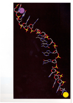


© Copyright 2026