
Room to Move: Why Some Industries Drive I Jaap W.B. Bos
Room to Move: Why Some Industries Drive the Trade-Specialization Nexus and Others Do NotI Jaap W.B. Bosa,∗, Lu Zhangb a Maastricht University School of Business and Economics, 6200 MD Maastricht, The Netherlands School of Economics, Utrecht University, 3512 BL Utrecht, The Netherlands b Utrecht Abstract In this paper, we investigate which industries drive the trade-specialization nexus in the European Union over the 1997-2006 period. We follow Melitz (2003), and argue that industries need 'room to move' in order for increasing trade openness to translate into increased specialization. Our paper finds that the true drivers of the trade-specialization nexus are productive firms, who benefit from the increase in trade-openness and can appropriate resources from less productive firms. This causes the industry in which they operate to expand, at the expense of other industries, in which there is no room to make such moves. We argue and find that the potential for reallocation in industries determines whether there is a trade-specialization nexus; in industries with little potential for reallocation, increased trade openness has no or a negative effect on that industry’s share of total value added. As a result, the trade-specialization nexus is driven by a small number of industries, who nevertheless have a significant impact on concentration patterns. Keywords: Trade Integration, Specialization, Reallocation, Conditional Latent Class Model JEL: C23 1. Introduction Over the past two decades, economic integration, mirrored by a rapid growth in international trade, has had a strong impact on specialization in the European Union (EU).1 The economic literature has a long tradition of analyzing what drives the relationship between trade and specialization. Classical trade theories predict that trade integration will result in increasing specialization in sectors where a country has a comparative advantage due to cross-country differences in technology or factor endowment (Ricardo, 1817; Ohlin, 1933). New trade theories stress the importance of increasing returns to scale and product differentiation in facilitating intra-industry trade and predict that international trade will induce a shift of increasing-return industries towards countries with good market access, i.e., the core (Krugman, 1979, 1980). New economic geography theories emphasize agglomeration forces I We thank the participants at the 2012 Nederlandse Economendag in Amsterdam (The Netherlands), the 2012 European Trade Study Group Conference in Leuven (Belgium), the 2011 European Workshop on Efficiency and Productivity Analysis in Verona (Italy), the 2010 Asia-Pacific Productivity Conference in Taipei (Taiwan) and the 2010 North American Productivity Workshop in Houston (United States) for their valuable comments. We also thank seminar participants at Copenhagen University and Utrecht University as well as Victoria Purice for most helpful comments. We thank Caroline Studdert for excellent editorial services. Lu Zhang gratefully acknowledges the financial support from the Netherlands Organization for Scientific Research (NWO). The usual disclaimer applies. ∗ Corresponding author. Email addresses: [email protected] (Jaap W.B. Bos), [email protected] (Lu Zhang) 1 During the 1997 to 2006 period, all EU14 countries except Portugal have experienced a significant increase in industrial specialization. Particularly large increases are observed in United Kingdom, Austria and France, where Gini coefficients have risen by 14.5, 10.1 and 9.8 percent, respectively. The Gini coefficient in Portugal has decreased by 5.6 percent. 1 and suggest a non-monotonic relationship between trade liberalization and location of economic activities, depending on the level of trade costs (Krugman, 1991; Venables, 1996).2 Much less is know about who drives the relationship between trade and specialization. Melitz (2003) argues that within-industry reallocation of resources contributes to a major part of industry productivity growth following increases in trade openness.3 Bernard et al. (2007) extend Melitz (2003) by combining his setup with a standard Heckscher-Ohlin model, showing that within-industry reallocation, induced by the decline of trade costs as described in Melitz (2003) is stronger in comparative advantage industries than in comparative disadvantage industries. Since the imposition of constant mark-ups seems at odds with the pro-competition effect of trade, Melitz and Ottaviano (2008) introduce quasi-linear firm preferences to generate endogenous mark-ups that vary with firm productivity, market size and international trade. In their model, intra-industry reallocation is magnified by the fact that by lowering the level of protection, trade intensifies product market competition, reduces prices and mark-ups, and forces high-cost firms to exit. In addition to exporting, importing (Kasahara and Lapham, 2008) and engaging in foreign direct investment (FDI) (Helpman et al., 2004) have also been considered as channels to induce within-industry reallocation. In this paper, we investigate which industries are driving the trade-specialization nexus. We follow Melitz (2003), and argue that industries need 'room to move' in order for increasing trade openness to translate into increased specialization. We are further motivated by a growing body of recent theoretical and empirical literature that has highlighted the importance of analyzing firm-level adjustment processes in response to the openness to foreign trade (Tybout and Westbrook, 1995; Pavcnik, 2002; Trefler, 2004; Bernard et al., 2006; Eslava et al., 2009). These studies have documented the existence of a substantial degree of firm-level heterogeneity even within narrowly defined industries.4 A substantial part of the effect of international trade is channeled into the reallocation of resources within the industry, which in turn shapes the industry aggregates. In our paper, the true drivers of the trade-specialization nexus are productive firms, who benefit from the increase in trade-openness and can appropriate resources from less productive firms, thus causing the industry in which they operate to expand, at the expense of other industries, in which there is no room to make such moves. We argue and find that the potential for reallocation in industries determines whether there is a trade-specialization nexus; in industries with little potential for reallocation, increased trade openness has no effect, or a negative effect, on that industry’s share of total value added. As a result, the trade-specialiation nexus is driven by a small number of industries, which nevertheless have a significant impact on concentration patterns. To analyze who drives the trade-specialization nexus, we use a panel data set consisting of 330,852 manufacturing firms spanning 18 industries in 14 EU countries over the period 1997-2006. After we estimate firm-level economies of scale and technical efficiency levels for each industry, we use the initial dispersion in both productivity measures to endogenously sort each industry into one of two classes. We observe a positive, inverted-U shape trade-specialization relationship for the high-potential class; the same relationship is insignificant or slightly negative for the low-potential class. Our analysis is further supported by a detailed instrumentation strategy, a novel way to identify the treatment effect of an increase in trade openness, and an elaborate robustness analysis. In addition, we verify the relevance of our approach by demonstrating how closely our predicted specialization patterns match the actual specialization that took place in the EU over our sample period. Our study is related to two strands of literature. The first strand has examined the dynamic relationship between trade liberalization and specialization patterns. For instance, Beine and Coulombe (2007) study the impact of trade liberalization between Canada and the US and find a positive short-run relationship and a negative long-run relationship, i.e., short-run specialization and long-run diversification. Crabbé 2 Lower trade costs result in the agglomeration of economic activities into fewer locations. However, a further reduction in trade costs leads to a geographical dispersion of activities when labor mobility across sectors exhibits finite costs. 3 He demonstrates this by building a dynamic industry model incorporating firm heterogeneity into Krugman’s (Krugman, 1979) monopolistic competition framework. 4 Bartelsman et al. (2004) have made important advancements in compiling firm-level panel data across a considerable number of countries and conducting international comparison of productivity and firm-level dynamics, although the role of trade-induced reallocation has not been explicitly examined. 2 et al. (2007) conduct a similar analysis for 13 CEEC countries and find that trade liberalization leads to long-run specialization. Compared with both studies, our analysis benefits from having far less potential for aggregation bias. The second strand of the literature relevant to our work concerns the intra-industry reallocation process in response to trade liberalization. Pavcnik (2002) finds that trade liberalization in Chile during the 1979-1986 period has had substantial reallocation and productivity effects. Trefler (2004) examines the reallocation and productivity effect of the Canada-U.S. Free Trade Agreement (FTA) on Canadian industries, and finds that industries with the deepest Canadian tariff reduction experienced a reduction in employment by 12 percent plus a 15 percent increase in industry labor productivity due to the contraction of low-productivity plants. For the US, Bernard et al. (2006) demonstrate that productivity gains are most pronounced in industries where trade barriers have declined the most.5 To the best of our knowledge, our study is the first contribution to the literature on how firm-level dynamics affect the integrationspecialization nexus, based on a unique sample of EU manufacturing firms. The remainder of the paper proceeds as follows. Section 2 presents the models used and the econometric strategy. Section 3 presents the data and the measures proposed. Section 4 discusses the results. Finally, section 5 summarizes and concludes. 2. Methodology In this section we first present our empirical model. An conditional latent class framework is employed to examine the heterogeneous effect of trade integration on specialization, conditional on the withinindustry potential for reallocation. Next, we discuss methodological concerns and our identification strategy. 2.1. Empirical Framework In the simplest possible manner, the trade-specialization nexus can be described as follows: Sot = f ( Tot ) , (1) where Sot = ∑ (Siot )2 and Siot is nominal industry value added as a percentage of a country’s total value iot added, VA VAot , i.e., the market share of that industry. Tot is a country-level measure of trade liberalization. Most neoclassical trade theories, with reference to the theory of comparative advantage, predict a positive relationship between trade liberalization and industrial specialization.6 Along the lines of the ∂Sot trade-specialization nexus, we expect a positive relationship, ∂T > 0 (Dornbusch et al., 1977; Sapir, 1996; ot Brülhart, 2001; Longhi et al., 2003; Riet et al., 2004). But what drives the relationship? Or, rather, who drives the relationship? Since Melitz (2003), we know that intra-industry reallocation of resources contributes to a major portion of industry productivity growth following increases in trade openness. Melitz (2003) also teaches us that actual reallocation is expected to be endogenous to trade openness. Important for the purposes of our analysis is the potential for reallocation, as trade openness can act as the catalyst that facilitates the realization of this potential, as reflected in changes in specialization. Put differently, we expect the trade-specialization nexus to be driven by those industries that have the scope to reallocate resources, thus benefiting from the increased trade openness. In order to find out whether this is indeed the case, we can apply the above equation to industry-level data:7 Siot = f ( Tiot ) (2) 5 For a comprehensive survey, see Tybout (2000). trade costs result in a narrowing non-traded sector; it is therefore cheaper to import goods than to produce them domestically. Thus resources are freed up and used more intensely in fewer activities (Dornbusch et al., 1977). 7 To understand why, consider aggregating equation (2) across all industries i at time t for each country o. Post-multiplying by 6 Falling Siot gives (Siot )2 = f ( Tiot × Siot ). The summation over industries i = 1, ..., I then gives ∑iI=1 (Siot )2 = f ∑iI=1 ( Tiot × Siot ) . Since 2 ∑iI=1 ( Tiot × Siot ) is the value added weighted average trade openness, equal to Tto , and ∑iI=1 (Siot ) is a country’s Hirschman Herfindahl at time t, equal to Sto , the latter equation is equivalent to equation (1). 3 where Siot is a measure describing the extent to which a country o at time t specializes in industry i, and T is that industry’s trade openness at the same time. According to the trade-specialization nexus, we now ∂Siot > 0. In line with Redding (2002), we rely on neoclassical trade theory and define Siot as nominal expect ∂T iot iot industry value added as a percentage of a country’s total value added, VA VAot . Using the simplest possible parametrization, while allowing for a non-linear effect in the spirit of new economic geography theories (Krugman, 1991; Venables, 1996), we can write: 2 + β0 Ziot + ε iot Siot = β 0 + β 1 Tiot + β 2 Tiot (3) where β0 is an 1 × n parameter vector; Z is a n × 1 vector of control variables, where we include the size of the manufacturing sector and industry-level labor productivity. In the simple example in equation (3), we pool data for all industries, in all countries. When can we ∂Siot = β 1 + 2 ∗ β 2 Tiot > 0, when we apply equation (3)? Clearly, expect to get a positive marginal effect, ∂T iot this is the case if ∂Siot ∂Tjot is positive for all industries in all countries and Tiot is increasing in roughly half of the sample, whereas it is decreasing in the other half of the sample. To understand why, consider the fact that - analogous to our simple two-industry example above - an increase in the share of industry i in each country is matched by a decrease in the share of industry j, and vice versa. So if the underlying relationship between specialization and trade openness is of the same sign and magnitude in all industries, trade openness has to fall in approximately half of the sample, assuming it increases in the other half. In practice, as we shall also show for our sample, trade openness has increased over time in most industries, rendering it impossible to find a positive relationship between specialization and trade openness under the assumptions just mentioned. There is, however, another possibility: even if Tiot is non-decreasing in all (or most) of the sample, we can still find a positive β 1 if the sign and/or magnitude of the underlying relationship between specialization and trade openness is not the same for all industries in a country. More specifically, in that case the relationship must be positive for those industries that have increased their share of the total value added, and negative or not significantly different from zero for all other industries. The question then becomes how we can identify which industries are able to increase their share of the total value added as a result of the increase in trade openness. From Melitz (2003), we know that these should be the industries which have a large enough potential for reallocation. Let us call these industries high-potential (HP) industries, as opposed to low-potential (LP) industries. Let eiot be the marginal effect of openness on specialization, i.e. eiot = ∂Siot ∂Tiot For any industry i in country o at time t, there are two possible values for eiot : HP eiot if HPiot = 1; eiot = LP eiot if HPiot = 0, (4) (5) HP > 0 ≤ e LP . What is the observed e where eiot iot when we pool data and estimate equation (3)? Following iot Angrist and Pischke (2008), it can be written in terms of the potential values eiot can take: LP HP LP eiot = eiot + eiot − eiot HPiot , (6) HP − e LP is the causal effect of being an HP industry. where eiot iot In practice, of course, HP is a latent variable. However, we can estimate that variable using a sorting equation, which assigns each industry i in country o at time t to either the HP industries or the LP industries 4 class. If we let θiot measure the odds of being an HP industry, conditional on the set of variables in the vector Viot , then exp Viot θ HP . (7) θiot = exp (Viot θ HP ) + exp (Viot θ LP ) Of importance in the light of our analysis is the vector Viot : it should contain covariates that predict whether an industry will be able to reallocate from its least productive to its most productive firms, thus benefiting from the opportunities that have arisen as a result of increased trade openness and resulting in an increased share of this industry in total production or value added. In Section 3, we explain the variables contained in Viot in detail. For now, we note that these variables capture productivity differences at the firm level within each industry i in country o at time t, at the start of our sample period. As a result, Viot captures the potential for reallocation, and is then used to estimate θiot . Once we know the prior probability, for each industry i in country o at time t, of being part of the HP class, we can estimate θiot with a logit model. We can then also allow for endogenous sorting of each industry i in country o at time t into each of the classes, and can rewrite equation (3) as follows: 2 Siot = β 0| HP,LP + β 1| HP,LP Tiot + β 2| HP,LP Tiot + β0HP,LP Ziot + ε iot| HP,LP (8) where each class, HP and LP, has its own parameter vector β. In other words, β 0 , β 1 , β 2 and β0 are allowed to differ across classes. As a result, eiot is now class-specific, as in equation (5). To obtain those parameter estimates, equation (8) is jointly estimated with equation (7) using an iterative procedure with an expectation-maximization (EM) algorithm, following Greene (2007). In this procedure, the unconditional likelihood for each industry i in country o at time t is obtained as a weighted average of its class-specific likelihood using the prior probabilities of being in classes HP and LP as the weights. Each industry i in country o at time t is thereby placed in the class where it contributes the most to the total likelihood of the estimated system, which is being maximized.8 Although it is natural in light of our investigation to estimate equations (8) and (7) for two classes, we need to identify the optimal number of classes. Orea and Kumbhakar (2004) suggest using the Akaike Information Criterion (AIC) and Schwartz Bayesian Information Criterion (SBIC), where the preferred specification has the lowest AIC and/or SBIC. 9 In practice, the class allocation may exhibit a certain degree of persistence and is likely to be stable. However, following Bos et al. (2010), industries can switch classes over time, since an industry’s allocation in a given period is ex ante independent of its allocation in other periods. We can thus study how the changes in the potential for reallocation affect the dynamics of the trade-specialization relationship. In addition, adding this flexibility to the model may allow us to identify causality, as explained below. To summarize, we employ a conditional latent class model to examine the heterogeneous relationship between trade integration and specialization in K endogenously determined groups of industries. The group membership probabilities are conditional on the potential for reallocation by exploring firm-level efficiency and scale characteristics within industries. 2.2. Identification of causality In order to analyze whether there is a causal effect of trade openness on specialization, we need an identification strategy. Obviously, the simple correlation between trade openness and specialization can not be interpreted as evidence of causality because specialization itself also affects trade. For example, 8 The sum of all unconditional likelihoods over all industries i in countries o at time t is maximized with respect to the parameter vectors for each class in equation (8) and the parameters in the sorting equation (7). With these parameter estimates, a posterior estimate of the class membership probability for each industry i in country o at time t can be computed using Bayes’ theorem. Each observation is assigned to a particular class with the largest posterior probability. The posterior estimate of the parameter vector β can also be obtained by multiplying the posterior membership probability. 9 Theoretically, the maximum number of classes is only restricted by the number of cross-sections, i.e., the number of observations in the data. However, empirically an over-specification problem limits the existence of a large number of classes. 5 Imbs (2004) demonstrates a negative relationship running from specialization to trade, as a result of intraindustry trade. Furthermore, unobserved industry/country characteristics can influence both trade and specialization/production - such as industrial policies or demand shifts that are difficult to measure and control for.10 Given these concerns, identification based on the direct impact of trade openness on specialization will yield inconsistent estimates. As a first step to proper inference, we observe that the three-dimensional panel that we have (industry, country, time) makes it possible to include a wide array of fixed effects in order to control for the unobservables and resolve omitted variable bias concerns to a large extent. In particular, the possibility to introduce interacted fixed effects enables us to sweep out a much wider range of omitted variables. For example, industry × time (it) effects would not only absorb industry fixed effects, but also the average effects of time-varying industry characteristics, such as economies of scale, research-orientation, technology level and labor intensiveness (Midelfart-Knarvik et al., 2000; Longhi et al., 2003). Similarly, country × time (ot) effects eliminate all time-varying country characteristics that affect specialization, such as market potential, R&D spending or labor abundance (Midelfart-Knarvik et al., 2000; Longhi et al., 2003). Furthermore, the industry × country effects capture any peculiar characteristics that vary for each industry-country combination and stay constant during our sample period 1997-2006. Therefore, in our specification, we control for all these three types of interactive fixed effects, namely industry × time, country × time and industry × country by demeaning both sides of equation (8) along these three dimensions. However, all these fixed effects may still not eliminate factors at the industry × country × time dimension. To deal with this concern, we incorporate output per worker as a control variable to correct for any technological shifts at the industry × country × time level that could affect specialization (López and Sánchez, 2005). Essentially, our identification strategy thereby exploits the time variation within each industry in each country, in line with our aim of exploring the role of (time-varying) firm dynamics in the trade-specialization relationship. Furthermore, we endeavor to establish a causal link between trade openness and specialization by addressing reverse causality in three ways. The first two methods involve instrumental variables, whereas the last method involves a less commonly used strategy that is closely related to our use of the latent class model. 2.2.1. Instrumentation to control for endogeneity First, we construct an instrumental variable for trade openness at the industry level, using gravity estimates. This methodology is developed by Frankel and Romer (1999) in the context of studying the relationship between trade openness and growth at the country level, and has been extended by Di Giovanni and Levchenko (2009) to the industry level. For each industry, Di Giovanni and Levchenko (2009) estimate a (cross-section) gravity equation to predict bilateral trade openness by means of distance, population, language, land-border, land area and land-locked status. The summation of the predicted trade openness across trading partners yields an industry-level natural openness measure, i.e., predicted trade volume as a percentage of output not only in each country, but also in each industry within each country. Gravity estimates provide a good instrumental variable as the geographical variables used are plausibly exogenous and highly correlated with the actual trade openness. Our point of departure is to extend Di Giovanni and Levchenko (2009) within a panel framework. Our approach corrects for important mis-specifications of gravity models commonly used in the literature, and yields a time-varying industry-level natural openness. The latter is particularly appealing in our context as we are interested in the evolution of the effects of trade openness on specialization over time, given the fact that trade barriers and costs have decreased significantly in the EU during the past few decades (Chen and Novy, 2011). Second, we construct an industry-specific time-varying trade integration measure proposed by Chen and Novy (2011). They derive a micro-founded measure of bilateral sector-specific trade frictions, i.e., the inverse of bilateral trade integration. They model disaggregated trade flows at the industry level in a gravity framework, allowing trade costs to be heterogeneous across industries. This measure is proven to 10 Another reason is that specialization is theoretically linked to the factor content of trade, as an industry that has a large share in GDP is likely to be an exporting sector. So the relationship between production patterns and endowments is not independent of the relationship between trade and endowments. 6 be theoretically consistent with a wide range of trade models and correlated with a large set of observable trade cost proxies.11 Appendix A lays out the details of our approach. 2.2.2. Identifying treatment effects through latent class modeling Once we have instrumented, as explained above, we have obtained unbiased estimates of the marginal effect of trade openness on specialization, for both the high-potential class and the low-potential class, respectively. But can we also infer the treatment effect from being in the high-potential class from this? Put differently, can we interpret the difference between these marginal effects as the causal effect of openness on specialization for the high-potential class? As it turns out, our modeling set-up - a latent class model, with possible class switches and instruments for trade openness - indeed allows us to identify this treatment effect, provided the resulting set-up mimics a quasi-natural experiment. To see when this is the case, it is necessary to reconsider equation (6), which showed the observed marginal effect of openness on specialization, eiot , when we pool data and estimate one equation for the whole sample. Imagine for a moment that industries are randomly assigned to the HP and LP class. In HP − e LP is the causal effect of being an HP industry. On average, this effect can be written as that case, eiot iot (Angrist and Pischke, 2008): HP LP E [eiot | HPiot = 1] − E [eiot | HPiot = 0] = E eiot | HPiot = 1 − E eiot | HPiot = 1 (9) LP LP + E eiot | HPiot = 1 − E eiot | HPiot = 0 , where h i h i h i HP LP HP LP E eiot | HPiot = 1 − E eiot | HPiot = 1 = E eiot − eiot | HPiot = 1 is the average causal effect of begin an HP industry on those that were indeed an HP industry. And h i h i LP LP E eiot | HPiot = 1 − E eiot | HPiot = 0 (10) (11) is the selection bias. Under what conditions can we calculate both effects from applications of our latent class model, where we indeed obtain separate parameter estimates for HP and LP? Simply put, this is the case if the assignment to the classes is random, in which case we can consider the HP class the treatment group and the LP class the control group. In light of our conditional latent class model, this means that the covariate vector Viot we employ in applications of equation (7) should be uncorrelated with our specialization measure if some industries indeed switch classes over time, we can even claim LP Siot . In addition, | HPiot = 1 , i.e., the marginal effects of openness on trade for a HP industry that is in the to measure E eiot LP class. In section 4.4, we use these observations to measure both the treatment effect as well as selection bias, and test the underlying assumptions. 3. Data We use an extensive data set that contains firm-level, industry-level and country-level data for 18 manufacturing industries in 14 EU countries over the period 1997-2006. For the firm-level data, we have compiled a comprehensive data set based on annual editions of the AMADEUS (Analyze Major Databases from European Sources) database.12 We supplement this data set with industry- and country-level data from 11 It is worth noting that measurement error in independent variables can lead to misleading inferences in regression-type applications. Although employing the instrumental variable of trade openness we have constructed might introduce measurement errors in our estimations, using Chen and Novy (2011)’s measure does not have this problem. Therefore, we presents results using both approaches and are confident that measurement errors do not pose a serious challenge to the validity of our results. 12 One of the characteristics of the AMADEUS database is that each edition only includes surviving firms. In addition, as time has gone by, the coverage of AMADEUS has increased. By using all annual editions of AMADEUS, and compiling the dataset both backward looking (to reduce survivorship bias) and forward looking (to increase the coverage), we are able to construct the most comprehensive firm-level data set of European manufacturing firms. 7 various sources. Industry-level data - disaggregated at NACE 2-digit - on value added, output, imports, exports and employment are taken from the OECD (2008) Structural Analysis Database (STAN). Countrylevel data on manufacturing GDP and GDP are retrieved from the World Bank (2008) World Development Indicators (WDI). Except for employment, all data are reported in current U.S. dollars. The industries and countries included in our sample are listed in Table A.1 and Table A.2 in Appendix A, respectively. Below, we explain how each of the variables we use is constructed. Our aim is to construct an industry-specific specialization index, since we are primarily interested in examining the heterogeneity of the trade-specialization relationship across industries. Our starting point is Redding (2002), who uses neoclassical trade theory to derive a specialization measure (spe), defined as nominal industry value added as a percentage of a country’s total GDP.13 In equation (12), we express Redding (2002)’s measure as the product of an industry’s share of a country’s manufacturing value added (S) and manufacturing’s share of a country’s GDP (MS). In our estimations, we log transform each of these components, which then allows us to include the log of MS as a control variable and the log of S as our dependent variable. In this manner, we isolate the impact of increased trade openness within manufacturing industries from the overall decline in manufacturing activity. manufacturing speiot = VAot VAiot VAiot = × manufacturing GDPot GDPot VAot = Siot × MSot (12) As a robustness test, we also construct an additional measure of specialization, S0 . This measure is the log of the normalized value added, where for each country, normalization is based on the value added of the food industry (NACE 15-16), which is set at 100 at the beginning of our sample, in 1997. Essentially, this normalized variable captures the changes of industry composition within a country over time. We describe the results using this variable as a robustness check in Appendix D. From Table 1, we observe that there is a wide variation in shares across manufacturing industries, as expected. The variation of the share of the manufacturing sector as a whole, however, varies much less. In addition, we control for industry-specific, time-varying productivity by including output per worker (Y/L), which varies significantly across our sample. In a similar vein, we measure trade integration at the industry level. The existing literature distinguishes between de jure and de facto measures of trade integration (Sachs and Warner, 1995; Wacziarg and Welch, 2008). De jure measures capture the extent of government restrictions on trade flows, whereas de facto measures quantify the degree of openness through realized trade flows. Since de jure measures are typically not available at the industry level, we mainly rely on the measure of de facto openness (T), defined as the ratio of industry imports and exports to output (Di Giovanni and Levchenko, 2009). Table 1 contains descriptives of both T and its instruments T 0 and T 00 , described in the previous section. The main observation from comparing the three trade openness measures, is that the measure based on Chen and Novy (2011) has far less variance than the other two measures. The correlation between openness and natural openness is 0.9, whereas the correlation between openness and trade integration is 0.2. Both correlations are significant at the 1 percent level. To capture the intra-industry potential for reallocation, we need a set of conditioning variables Viot . Since this type of reallocation takes place between firms in the same industry, we require firm-level observations to construct industry-level measures. Our objective is to show the extent to which the most productive firms in an industry can grow by appropriating the assets of the least productive firms. Therefore, we need to measure the dispersion in productivity within each industry in each country. We measure the productivity of each firm in two ways. First, and most closely related to Melitz (2003), we estimate each firm’s economies of scale. Second, and based on the same estimations, we estimate each firm’s efficiency. Our primary measure of dispersion is the ratio of the productivity of firms in the top quantile (i.e., with the highest economies of scale, or the most efficient) to the productivity of firms in the bottom quartile 13 This measure has the advantage of being theory-consistent, in contrast with ad-hoc definitions of specialization that have been used by other authors, such as the indexes of revealed comparative advantage, pioneered by Balassa (1965). 8 V Z T S Table 1: Descriptive statisticsa a Variable Description Source Mean Min Max Std S Specialization OECD STAN 5.877 0.016 23.585 4.267 S0 Normalized specialiation OECD STAN 1.458 -4.110 3.161 0.905 T Openness (imports+exports)/value added 153.290 16.677 5735.303 405.529 T0 Natural openness (instrument) Di Giovanni and Levchenko (2009) 165.858 11.655 9344.317 562.117 T 00 Trade integration (instrument) Chen and Novy (2011) 2.273 0.710 6.206 1.017 Y/L Labor productivity, $1000 OECD STAN 281.449 17.895 8036.795 522.882 MS Manufacturing share OECD STAN 18.311 8.715 26.452 4.071 E25/75 Efficiency dispersion, 25/75 ratio AMADEUS, own calculations 1.151 1.001 13.085 0.279 E10/90 Efficiency dispersion, 10/90 ratio AMADEUS, own calculations 1.435 1.001 13.516 0.576 Eσ Efficiency dispersion, standard deviation AMADEUS , own estimations 0.112 0.001 0.365 0.038 S25/75 Scale dispersion, 25/75 ratio AMADEUS, own calculations 1.035 1.002 1.109 0.014 S10/90 Scale dispersion, 10/90 ratio AMADEUS, own calculations 1.070 1.003 1.174 0.026 Sσ Scale dispersion, standard deviation AMADEUS, own calculations 0.028 0.002 0.073 0.009 Et=0 Initial efficiency level (weighted) AMADEUS, own calculations 0.773 0.176 0.910 0.082 S t =0 Initial scale level (weighted) AMADEUS, own calculations 1.091 0.886 1.623 0.149 Number of observations is 2,138; based on specifications given in Table 3; Std=standard deviation. (i.e., with the lowest economies of scale, or the least efficient), the 25/75 ratio. To check the robustness of our results, we also use two other measures of dispersion, the 10/90 ratio and the standard deviation of scale and efficiency, described in the robustness analysis in Appendix D. To control for the initial level of industry efficiency/scale, for each industry we take the weighted-average of efficiency/scale by the firm’s total assets. We estimate each firm’s economies of scale and efficiency as follows. First, we estimate a stochastic production frontier for each industry, described in detail in Appendix B. Our approach has three distinct features. First, by estimating a translog production function, we allow for increasing, decreasing and constant constant economies of scale, within an industry, at any time. Second, by estimating this production function using stochastic frontier analysis (SFA), we can also measure efficiency, i.e., the extent to which firms with the same economies of scale and input levels produce different levels of output. In our approach, the error term of that stochastic production frontier is composed of two parts (Aigner et al., 1977; Battese and Corra, 1977; Meeusen and Broeck, 1977): a one-sided component with a truncated distribution that captures inefficiency, as well as a systematic component that allows for measurement errors or other random shocks around the production frontier. Third, we account for systematic differences in production technologies, which may otherwise be wrongly labeled as inefficiency (Orea and Kumbhakar, 2004), by estimating true fixed effects frontiers (Greene, 2005), with firm- and country-fixed effects for each industryspecific frontier. In so doing, we still assume that firms that produce similar products and thereby operate in the same industry can be benchmarked against each other, even if they operate in different countries. Put differently, even though we allow for structural differences in output (and productivity) between firms that operate in the same industry, but in different countries, we assume that these firms have access to the same production technology.14 For our firm-level productivity estimations, we use the all-companies module of AMADEUS, a database provided by Bureau Van Dijk Electronic Publishing. This pan-European database contains detailed financial and business data on more than 10 million public and private firms in 44 European countries. The homogeneity of the data collecting process across countries and its fairly complete coverage, especially of privately held firms makes it well suited for our analysis. Our sample consists of 330,852 manufacturing 14 Bos et al. (2010) endogenize the allocation of European manufacturing industries in a low- and high-technology class. Although, in their paper, the same industry can belong to one class in one country and another class in another country, in their Table A4 they show that most industries cluster in the same class, confirming that technology difference, in EU manufacturing, are industry- rather than country-specific. 9 firms across 14 EU countries over the 1997-2006 period. We choose manufacturing industries because in contrast to services, they are more involved in trade and more responsive to trade integration.15 We group all firms into 18 industries to ensure a sufficient number of firms in each industry-country combination, and compatibility with other industry-level data. The choice of countries is based on the quality of firmlevel coverage.16 To estimate the stochastic production frontier, we use raw data on gross value added, tangible fixed assets and number of employees to construct firm-level output (Y), capital (K) and labor (L), respectively. Appendix C describes the AMADEUS database, the sample selection procedure and the construction of our variables in details. Table 1 summarizes the definitions, sources and descriptive statistics of the main variables used in our analysis, respectively. In Table 1, we observe that the most efficient quartile of firms is on average 15% more efficient than the least efficient quartile. However, if we move one standard deviation (0.279) above this average, the difference has increased to more than 40%. Results are similar for the other two efficiency dispersion measures. Average efficiency at the beginning of the sample period is 77.3%, indicating that the average firm should be able to increase its output by 22.7% without increasing its use of inputs. The average economies of scale at the beginning of the sample period are 1.091, indicating that the average firm experiences increasing returns to scale, and can increase its output by 1.091% by increasing its inputs by 1%. The top quartile firms operates with economies of scale that are on average 3.5% larger than the bottom quartile, although this difference can increase to more than 10% for some industries. As explained in the previous section, for the purpose of our analysis, we aim to measure the potential for reallocation in each of the industries in each of the countries. But how valid are our measures introduced above? In order to validate them, we also calculate the actual degree of reallocation that takes place in each industry in each country over the sample period, using a decomposition method suggested by Olley and Pakes (1996). Consider the following decomposition of efficiency and scale for an industry i in country o at the period t: Siot = ∑ w jiot Sjiot = Siot + ∑(w jiot − wiot )(Sjiot − Siot ) (13) ∑ w jiot Ejiot = Eiot + ∑(w jiot − wiot )(Ejiot − Eiot ) (14) j Eiot = j j j where j indexes firms, and S and E refer to efficiency and economies of scale, respectively. In equation (13), Siot represents the value-added weighted average economies of scale in industry i in country o at time t and Siot the unweighted average economies of scale. Equation (14) decomposes the value added weighted average efficiency into a first component that is size invariant, and a second component that is not. It is this second component in which we are interested, as it measures the sample covariance between economies of scale and value added. The larger this covariance, the higher the share of the value added that is produced by firms with higher economies of scale, and consequently the higher the industry-level economies of scale. The same applies to efficiency, in equation (14). Validating our measures of the potential for reallocation therefore involves assessing whether they are positively correlated with these two covariance terms. 4. Results In this section we present our results. First, we validate our measures of the potential for reallocation. Secondly, we examine whether the potential for reallocation has indeed driven the trade-specialization nexus. Thirdly, we explore the treatment effect from changes in trade openness, and fourthly we verify our results by comparing the actual shares of industries with the ones predicted by our model. 15 On average, manufacturing trade accounts for 80 percent of total merchandize trade in the EU. compare the total number of manufacturing firms and the number reported in OECD 2006 Structural and Demographic Business Statistics (SDBS) and select countries with more than 30 percent of firms covered. 16 We 10 4.1. Validation: actual and potential reallocation Do we find that industries with the most 'room to move' are also the ones where subsequently reallocation is most likely to take place? To validate our measures of the potential for reallocation, in Figures (1a) and (1b) we compare them to the actual reallocation that took place during our sample period. Figure 1: Potential vs. Actual Reallocation (b) Efficiency 1 1 1.1 1.02 Initial scale dispersion 1.04 1.06 Initial efficiency dispersion 1.2 1.3 1.4 1.08 1.5 (a) Scale −.05 0 .05 .1 Actual reallocation ( period average ) −.15 .15 −.1 −.05 0 .05 Actual reallocation (period average) .1 Two concurrent developments can be noted from these figures. First, we observe that higher levels of dispersion, signifying the greater potential for reallocation, are positively correlated with actual reallocation, especially for economies of scale.17 Second, as most covariance terms are positive, the reallocation is indeed in line with Melitz (2003), and can lead to the expansion of the industry in which firms are located. 4.2. How has the potential for reallocation driven the trade-specialization nexus? Our aim is to explain why some industries drive the trade-specialization nexus and others do not. Therefore, we start by determining the number of groups or classes of industries identified by our latent class model. Following Orea and Kumbhakar (2004), we estimate for two, three and four classes, respectively, and formally test using the Akaike and Schwartz Bayesian information criteria (AIC and SBIC, respectively). We do so using the natural openness measure following (Di Giovanni and Levchenko, 2009) and the trade integration measure from Chen and Novy (2011). As shown in Table 2, a specification with two classes is preferred for both measures, since this results in the lowest AIC and SBIC.18 Table 3 contains our estimation results. Panel B contains parameter equality tests and confirms what we have found so far: there are two distinct groups of industries, with significantly different parameters, both for trade openness and output per worker. Also, the parameters for variables used in the sorting equation are jointly significantly different from zero. Turning to Panel C, we see that the industries in the first class are characterized by a higher efficiency dispersion, a lower initial efficiency level, and a higher initial economies of scale level. Scale dispersion, however, is not higher in this first class. Most notable is the difference in the change in S, the manufacturing share of industries. In the first class, the change is between 2.5 and 3.2%, whereas it is approximately economies of scale, the slope coefficient is 0.61 and R¯ 2 is 0.13. a possible third group, we find that parameters are jointly not significant from zero, and the number of observations allocated in this additional group is rather small. 17 For 18 For 11 Table 2: Specification Tests of the Number of Groupsa Specification Two-group Three-group Four-group Likelihood 2313,357 2360,783 2415,082 Natural Opennessb Parameters AIC 15 14,507 25 34,467 35 54,421 SBIC 100,734 178,178 255,617 Likelihood 2195,605 2256,219 Trade Integrationc Parameters AIC 15 14,612 25 34,557 no convergence SBIC 100,83 178,269 a Akaike Information Criterion (AIC)= 2m − 2nLF (k ), Schwartz Bayesian Information Criterion (SBIC)= −2lnLF (k ) + mln(n); m is the number of parameters, n is the number of observations, LF(k) is the log likelihood for groups. The preferred specification has the lowest AIC or the lowest SBIC. See Orea and Kumbhakar (2004). Obs=2,318; b Di Giovanni and Levchenko (2009); c Chen and Novy (2011). -1.5% on average in the second class. Summing up, we henceforth refer to the first class as the highpotential or HP class, whereas the second class is referred to as the low-potential or LP class. The prior class probabilities (at data means) show that approximately between 7% and 9.2% of our sample belongs to the HP class, while the rest is assigned to the LP class. Table 3: The Trade-Specialization Nexus at the Industry Level Natural Opennessb High-potential Low-potential T 0.708 (0.218)*** -0.171 (0.067)** T2 -0.087 (0.017)*** -0.016 (0.007)** Output per worker 0.251 (0.066)*** 0.215 (0.021)*** Constant 0.001 (0.016) 0.000 (0.001) Scale dispersion 17.719 (8.137)** Reference Efficiency dispersion 5.940 (1.438)*** Reference Initial scale level 14.282 (1.426)*** Reference Initial efficiency level -4.144 (1.860)** Reference Constant -39.846 (8.665)*** Reference Prior class probability 0.092 0.908 Equality Tests Natural Opennessb Wald P-value Conclusion All parameters 14.519 0.000 Rejected T and T 2 15.306 0.000 Rejected Sorting variables 62.224 0.000 Rejected Class Characteristics Natural Opennessb HP LP P-valuee Scale dispersion 1.033 1.036 0.000 Efficiency dispersion 1.243 1.135 0.000 Initial scale level 1.333 1.048 0.000 Initial efficiency level 0.708 0.784 0.000 ∆S (%) 2.504 -1.511 0.001 Panel C Panel B Panel Aa Sorting Kernel Parameter Estimates Trade Integrationc High-potential Low-potential 0.396 (0.320) -0.261 (0.062)*** -0.421 (0.581) 0.077 (0.048) 0.408 (0.071)*** 0.285 (0.021)*** 0.007 (0.017) 0.000 (0.002) 14.066 (9.459) Reference 5.720 (1.411) *** Reference 14.998 (1.475)*** Reference -2.499 (2.576) Reference -38.130 (9.856)*** Reference 0.072 0.928 Trade Integrationc Wald P-value Conclusion 32.980 0.000 Rejected 19.362 0.000 Rejected 50.380 0.000 Rejected Trade Integrationc HP LP P-valuee 1.032 1.036 0.000 1.252 1.135 0.000 1.349 1.050 0.000 0.704 0.784 0.000 3.203 -1.548 0.000 a Standard errors in parentheses; significance at the 10/5/1 percent level (*/**/***); b Di Giovanni and Levchenko c Chen and Novy (2011); d Measured at data means; e Significance of difference in means. (2009); Of course, what remains to be seen is whether the trade-specialization nexus is indeed driven by the HP class, as we conjecture. We therefore turn to Panel A, which contains the parameter estimates. We start with the parameters in the sorting equation. Scale and efficiency dispersion increase the likelihood of being in the HP class, as expected. High initial scale levels make it more likely that an industry will be driving the trade-specialization nexus, whereas high efficiency levels make it less likely that an industry is in the HP class. Overall, results are more significant for the natural openness measure (Di Giovanni and Levchenko, 2009) than for the trade integration measure (Chen and Novy, 2011), which may be explained 12 by the latter’s low variance. In the top part of panel A, we find the parameter estimates for trade openness and labor productivity. As expected, labor productivity always has a positive relationship to an industry’s manufacturing share (López and Sánchez, 2005). More interesting are the results for trade openness: in line with our expectations, an increase in natural openness (Di Giovanni and Levchenko, 2009) increases an industry’s share in manufacturing in the HP class, whereas it has a negative, but much smaller effect in the LP class. Both effects are similar, but less significant for an increase in trade integration (Chen and Novy, 2011). For the HP class, results are in line with the trade-specialization nexus. For the LP class, increases in trade openness have a negative effect on an industry’s share in manufacturing. This is in line with López and Sánchez (2005), who find a negative relationship between openness and specialization for ten European countries. They assert that the convergence of industrial structures following the openness to foreign trade is consistent with the prediction of the Hechscher-Ohlin-Vanek theory: when factor prices are equalizing, the sources of comparative advantage arising from relative differences in factor prices disappear.19 Figure 2: Conditional Marginal Effect (b) Trade integration .5 1 −.2 0 Natural openness (in logs) marginal effect natural openness .2 −.1 0 .1 Trade integration (in logs) .2 .3 Marginal effect of trade integration −.4 0 .4 .8 1.2 0 2 4 6 Density of natural openness Marginal effect of natural openness −.4 −.2 0 .2 .4 .6 .8 1 Low−potential −.4 0 −.2 20 −.5 0 Natural openness (in logs) .4 5 10 15 Density of trade integration −1 0 −1.5 5 10 Density of trade integration Marginal effect of trade integration −.4 0 .4 .8 1.2 0 .5 1 1.5 2 Density of natural openness Marginal effect of natural openness −.4−.2 0 .2 .4 .6 .8 1 1.21.4 High−potential 15 (a) Natural openness −.2 95% confidence interval 0 .2 Trade integration (in logs) Marginal effect trade integration .4 95% confidence interval An interesting question to ask at this point is whether there is a saturation point beyond which further opening-up to international trade may not lead to increased specialization. Thus, the relationship between trade openness and specialization may no longer be positive for industries with very high levels of openness - a phenomenon that is identified in new economic geography theories (Krugman, 1991; Venables, 1996). These theories postulate a non-linear relationship between trade costs and location of economic activity. The decrease in trade costs induces firms to agglomerate into fewer locations, and a further decline in trade costs can result in geographical dispersion of activities when mobility across sectors exhibits a finite cost. Beine and Coulombe (2007) document a similar positive short-run relationship and a negative long19 Trade integration implies the creation of new exporting industries, which in turn leads to the expansion of aggregate production in those industries. This process could be driven by agglomeration forces and forward (large market)-backward (large input variety) linkages identified by new economic geography theories (Fujita et al., 2001). 13 run relationship between trade integration and specialization, i.e., short-run specialization and long-run diversification based on export data of Canadian regions. Therefore, in order to further assess the economic nature of the relationship between trade openness and specialization, we calculate the marginal effect of trade on specialization, i.e., the partial derivative of S with respect to T in equation (8), conditional on the level of trade openness T for both the HP and the LP class. Figure (2a) and Figure (2b) illustrate these conditional marginal effects and the corresponding 95 percent confidence intervals (Brambor et al., 2006). We infer for the HP class that although the effect of openness on specialization decreases as industries’ natural openness (in the top part of Figure (2a) and as trade integration increases (in the bottom part of Figure (2b). However the marginal effects remain positive and significantly different from zero in both cases. Thus, although there is some saturation with respect to trade openness, we do not find evidence of a threshold effect for the HP class. Things are even clearer for the LP class, where the marginal effect of natural openness (in the bottom part of Figure (2a)) and trade integration (in the bottom part of (2b)) is scarcely affected by changes in openness or integration and is consistently below zero. To check the robustness of our results, we first consider an alternative measure of specialization, i.e., (the log of) normalized industry value added. The results are reported in Panel A of Table D.1 in Appendix D. We find that they are qualitatively and quantitatively very similar to those in Table 3, despite of the lack of significance for two of the conditioning variables, namely scale dispersion and initial efficiency level. In addition, the division of the sample into a small HP and a large LP group resembles that of our main specification in Table 3. We then consider two other measures of dispersion, namely the 10/90 ratio and the standard deviation. Panels B and C of Table D.1 in Appendix D display the results. We find no significant changes from our main results, except that the scale dispersion and/or initial efficiency level loses its significance when the dispersion is measured as 10/90 ratio in Panel B of Table D.1. Similar results are found when using the standard deviation as the dispersion measure in Panel C of Table D.1. We find no evidence of changes in the main parameter estimates. But the power of our conditioning variables becomes somewhat weaker except for the initial economies of scale level - as the individual significance of three variables drops and the efficiency dispersion appears to have the "wrong" sign. These results may highlight the problems of using the standard deviation as the dispersion measure, because firm efficiency and economies of scale are not normally distributed within each industry. Overall, our results do not seem to be driven by the use of an alternative specialization measure, nor by the choice of a particular dispersion measure. To summarize, we find that the effects of trade openness on specialization appear to be very different in the HP and LP class. Using the potential for reallocation, i.e. the four conditioning variables jointly determines the allocation of an industry into either the HP or LP class. 4.3. How have the changes in the potential for reallocation affected the dynamics of trade-specialization nexus? An interesting question that arises is how the changes in the potential for reallocation affect the dynamics of the trade-specialization nexus. The distinctive features of our latent class model allows us to explore this question. In our modeling framework, the probability of belonging to a certain group depends on the average of all four conditioning variables. As a result, the changes in these variables can alter this probability. Therefore, we prefer here to permit industries to switch groups over time, rather than imposing the assumption that they are restricted to one group. Panel A in Table 4 shows the migration matrices, including the absolute number and percentage of group allocation changes over time. We can see both in panel A and B that the diagonal elements carry the largest percentage as would be expected, which indicates that the potential for reallocation hardly changes drastically. Transitions from the LP to HP group are rare. At the same time, transitions from the HP to LP group are more frequent, suggesting that if industries react to the trade openness by realizing the potential for reallocation, the remaining potential is reduced. Thus, these industries are more likely migrate to the LP group. 20 20 We checked whether the occurrence of transition is due to the fact that the conditional probability of an industry being in one group our model assigned is close to 50 percent, which is the conventional cut-off point in the multinomial logit model of equation 14 Table 4: Transitioning from High-potential to Low-potential Natural Opennessb To HP LP Total HP 215 58 273 (78.75) (21.25) (100) LP 56 1574 1630 (3.44) (96.56) (100) Total 271 1632 1903 14.24 85.76 (100) From From Panel A: Transition matrices Trade Integrationc To HP LP Total HP 193 55 248 (77.82) (22.18) (100) LP 54 1601 1655 (3.26) (96.74) (100) Total 247 1656 1903 (12.98) (87.02) (100) Panel B: Covariates Variable Efficiency dispersion Scale dispersion Initial efficiency level Initial scale level Mean Sign t-test 1.156 ** 1.038 + ** 0.766 + *** 1.155 *** KW *** *** *** *** Mean Sign t-test 1.146 ** 1.038 + *** 0.776 + *** 1.170 *** KW *** *** *** *** a Percentages in parentheses; significance at the 10/5/1 percent level (*/**/***); c Chen and Novy (2011); Di Giovanni and Levchenko (2009); d Measured at data means; e Significance of difference in means. b Most of the industry transitions, i.e., 31.03 percent of all cases, take place in the petroleum industry (18 out of 58), followed by 13.8 and 12.07 percent respectively in basic metals and electronic equipment industries. In terms of country divisions, 22.41 percent of industries transit from the HP to LP group in Hungary (13 out of 58), which seems not surprising given that CEEC countries are expected to be mostly affected by trade integration. They are closely followed by Portugal and Sweden with 12.07 and 10.34 percent (7 out 58 and 6 out of 58), respectively. However, we find no trends with regard to when these transitions occur. Panel B in Table 4 provides some further insights into why and how some industries migrate from the HP to the LP group. We examine whether the potential for reallocation is significantly lower for these switchers. More specifically, we employ t-test and Kruskal-Walllis test to test whether the four conditioning variables used to predict group membership differ significantly on average between industries that switch and those that stay in the HP group. A positive (negative) sign indicates the variable is higher (lower) than for the industries that stay in the HP group. For example, the first column in panel A indicates that efficiency dispersion is significantly lower (at 5 percent and 1 percent) than that of the average of the HP group. Overall, we find that the potential for reallocation of these switchers is significantly lower, evidenced by a lower efficiency dispersion, a higher efficiency level and a lower scale level. The scale dispersion appears to have the "wrong" sign, however. These results provide additional support for the saturation effect of trade openness: that the process of openness-driven-specialization is not monotonic, but rather, it is slowing down. 4.4. Exploring the treatment effect Now that we have identified that some industries are indeed driving the trade-specialization nexus, whereas others are not, an obvious next question is what the economic impact of changes in trade openness? In order to find out, we proceed with our approach in Section 2.2.2 and identify the treatment effect from trade openness. ??. However, the conditional probability of group membership is very high in almost all cases, i.e., above 90 percent. Therefore, the 15 Table 5: Randomization Scale dispersion Efficiency dispersion Initial scale level Initial efficiency level R¯ 2 F-test (p-value) -0.038 0.005 0.004 0.039 (0.041) (0.010) (0.019) (0.037) -0.0012 0.8275 a Regression of demeaned specialization (left-hand side variable in Table 3) on conditioning variables, without intercept. To that purpose, we start by investigating whether our latent class estimations can indeed be used to identify treatment effects and selection bias. For that to be the case, our model setup would have to mimic a clinical trial, i.e., industries’ share in manufacturing should be uncorrelated to the set of conditioning variables that we have used to determine class membership. In Table 5, we verify this by regression Siot on the set of conditioning variables. From the estimation results, we observe that not only are the variables jointly not significant, resulting in an R¯ 2 of -0.0012, but also none of the conditioning variables is significant in explaining specialization. Summing up, the assignment of industries to the HP or LP class makes ex post economic sense in terms of the observed effects of changes in trade openness on specialization, but is not ex ante set up to do so. Table 6: Identifying treatment effects and selection bias through a latent class framework HP LP E eiot | HPiot = 1 - E eiot | HPiot = 1 | {z average treatment effect on the treated 0.7094091c All industries Switchers All but switchers 0.7091428 0.7208096 - All industries Switchers All but switchers 0.3957784 0.3938258 0.3960658 - LP LP E eiot | HPiot = 1 - E eiot | HPiot = 0 } | Natural Opennessb -0.1707409 =0.88015 00 -0.1707898 = 0.8799326 -0.1686442 = 0.8894538 Trade Integrationc -0.2609595 = 0.6567379 -0.2606024 = 0.6544282 -0.2610120 = 0.6570778 {z selection bias } -0.1707409 -0.1707898 -0.1686442 - -0.1709663 -0.1710381 -0.1708486 = 0.0002254 = 0.0002483 = 0.0022044 -0.2609595 -0.2606024 -0.2610120 - -0.2608653 -0.2614941 -0.2602176 =-0.0000942 = 0.0008917 =-0.0007944 a Based on specifications estimated in Table 3. For example, for all industries, 0.7091789 = β 1| HP + 2 × β 2| HP × Openness = 0.708 + 2 ∗ −0.087 ∗ −0.0080981, where -0.0080981 is the average, demeaned natural openness for industries that are in the HP class. b Di Giovanni and Levchenko (2009), number of observations is 2,138 (all industries), 1,507 (switchers), 631 (all but switchers); c Chen and Novy (2011), number of observations is 2,138 (all industries), 380 (switchers), 1,758 (all but switchers). As a result, we can now identify the treatment effect and selection bias in Table 6. We do so for both natural openness and for trade integration. And in order to accommodate the fact that industries in our modeling framework can switch classes (and hence can go from treated to control group), we measure both effects for all industries, industries that switch and the remaining industries, respectively. For natural openness (Di Giovanni and Levchenko, 2009), we find a treatment effect of approximately 0.88, i.e., a one percent higher trade openness results in a 0.88% higher share of an industry in total manufacturing value added. Meanwhile, the selection bias is minimal and never more than 0.002. transition is not related to the flexibility of our model. 16 Results are qualitatively similar for trade integration (Chen and Novy, 2011), where a one percent increase results in a 0.66% higher share. Here, selection bias is also small, less than 0.001 in all cases. Given that natural openness increases by 2.504% on average in the HP class, and trade integration increases by 3.203%, these numbers are sizable, and explain why - despite the small number of industries (just below 10%) that are located in the HP class - the industries in the HP class are responsible for a large part of the structural changes we have observed in the countries in our sample. 4.5. Verification: actual and predicted industry shares Last but not least, we examine the predictive power of our model by looking at how well it predicts our specialization measure S, i.e., the industry shares. To do so, the top parts of Figure (3a) and Figure (3b) plot the predicted S against the actual S on the basis of equation (8) using natural openness and trade integration, respectively. It shows that the predicted S captures a considerable amount of variation embedded in the actual S (the correlation coefficient of 0.4 and 0.35, respectively). One point which deserves noting here is that since the specialization measure used in the estimation is in logs and demeaned, our model essentially predicts the deviation from the means. To retrieve the predicted shares, we add back the actual means (i.e., country-time, industry-time, and industry-country averages discussed in the methodology section). Figure 3: Predictability of the Latent Class Model (b) Trade integration (a) Natural openness Predicted vs. actual shares (log of, demeaned) Predicated (log of, demeaned) shares −.5 0 −.5 Predicated (log of, demeaned) shares 0 .5 .5 Predicted vs. actual shares (log of, demeaned) −.5 −.25 0 .25 Actual (log of, demeaned) shares .5 −.5 −.25 .5 20 Predicated shares 10 15 5 0 0 5 Predicated shares 10 15 20 25 Predicted vs. actual shares 25 Predicted vs. actual shares 0 .25 Actual (log of, demeaned) shares 0 5 10 15 Actual shares 20 25 0 5 10 15 Actual shares 20 25 The bottom parts of Figure (3a) and Figure (3b) plot the predicted industry shares (in levels) against the actual shares. It is clear from the figures that they are highly correlated (the correlation coefficient is 0.99 and 0.98, respectively), confirming the predictive power of our model. The caveat to bear in mind is that the "means" we take out may contain important information in explaining specialization, that is beyond the scope of our model. 17 To summarize, three main findings emerge from our analysis so far. First, the trade-specialization nexus is not homogeneous across all industries, nor is the relationship entirely unique for each industry. Instead, we find two distinctive groups of industries, and the potential for reallocation, i.e. the four conditioning variables, determines the assignment of each industry into a specific group. Second, the tradespecialization relationship is in stark contrast between the HP and LP group. We find that trade openness induces more specialization towards industries with high potential for reallocation. And the effect of trade decreases when trade openness is beyond a certain threshold. On the contrary, trade openness leads to less specialization in industries when their potential for reallocation is low. Lastly, some industries switch from the HP and LP group further when the remaining potentials are lower, furthering confirming that the trade-induced specialization process slows down over time. 5. Conclusion This paper has examined the role of reallocation as a driver of the trade-specialization nexus, and shown how firm dynamics constitute a channel through which trade liberalization affects the industrial composition within EU economies. We have proposed a conditional latent class model to examine the dynamic effect of trade liberalization on specialization across industries. The proposed model allows for a heterogeneous trade-specialization relationship across different endogenously determined groups of industries. The group membership probability is modelled as a function of four firm-based measures that encapsulate the intra-industry potential for reallocation, namely the dispersion of firm efficiency and scale and the initial level of industry average efficiency and scale. To obtain firm-specific efficiency and scale, we set up a model of production that permits the inefficient use of resources and estimate a stochastic production function. In order to overcome endogeneity problems, we employ two novel instrumentation strategies based on the exogenous geographic determinants of trade flows and a micro-founded measure of industry-specific trade frictions. Using a unique panel of manufacturing firms in 14 EU countries during 1997-2006, we have found evidence that the trade - specialization relationship differs markedly between two distinctive groups of industries and that the relationship depends on the potential for reallocation. We have shown that the potential for reallocation appears to be positively associated with the future actual reallocation observed in reality. On the one hand, an inverted U-shaped trade-specialization pattern has been found in one group of industries which are characterized by greater potential for reallocation, indicating that trade openness induces specialization at a decreasing rate. On the other hand, trade openness results in less specialization in the other group when the potential for reallocation is small. Our results are consistent with the theoretical and empirical evidence that international trade acts as a catalyst in facilitating the intra-industry reallocation of economic activity. Our findings have important policy implications. As reallocation is a key channel through which industries can benefit from trade liberalization, policies aimed at removing barriers in the factor and product markets are likely to enhance the reallocation of economic activity. The resulting gains in efficiency and economies of scale appear to be an important source of long-run competitiveness and economic growth in the EU. References Aigner, D., Lovell, C. A. K., Schmidt, P., 1977. Formulation and estimation of stochastic frontier production function models. Journal of Econometrics 6 (1), 21–37. Anderson, J. E., van Wincoop, E., 2003. Gravity with gravitas: A solution to the border puzzle. American Economic Review 93 (1), 170–192. Anderson, J. E., van Wincoop, E., 2004. Trade costs. Journal of Economic Literature 42 (3), 691–751. Angrist, J., Pischke, J., 2008. Mostly Harmless Econometrics: An Empiricist’s Companion. Princeton University Press. Princeton University Press. Balassa, B., 1965. Trade liberalisation and "revealed" comparative advantage. The Manchester School 33 (2), 99–123. Baldwin, R., Taglioni, D., 2006. Gravity for dummies and dummies for gravity equations. CEPR Discussion Papers 5850. Baltagi, B. H., Griffin, J. M., 1988. A general index of technical change. Journal of Political Economy 96 (1), 20–41. 18 Bartelsman, E., Haltiwanger, J., Scarpetta, S., 2004. Microeconomic evidence of creative destruction in industrial and developing countries. The World Bank Policy Research Working Paper Series 3464. Battese, G. E., Corra, G. S., 1977. Estimation of a production frontier model: With application to the pastoral zone of eastern australia. Australian Journal of Agricultural Economics 21 (3), 169–179. Beine, M., Coulombe, S., 2007. Economic integration and the diversification of regional exports: Evidence from the Canadian-U.S. free trade agreement. Journal of Economic Geography 7 (1), 93–111. Bernard, A. B., Jensen, J. B., Schott, P. K., 2006. Survival of the best fit: Exposure to low-wage countries and the (uneven) growth of u.s. manufacturing plants. Journal of International Economics 68 (1), 219–237. Bernard, A. B., Redding, S. J., Schott, P. K., 2007. Comparative advantage and heterogeneous firms. Review of Economic Studies 74 (1), 31–66. Bos, J., Economidou, C., Koetter, M., 2010. Technology clubs, R&D and growth patterns: Evidence from EU manufacturing. European Economic Review 54 (1), 60–79. Brambor, T., Clark, W., Gold, M., 2006. Understanding interaction models: Improving empirical analyses. Political Analysis 14 (1), 64–81. Brülhart, M., 2001. Growing alike or growing apart? Industrial specialization of EU countries. In: Wyplosz, C. (Ed.), The Impact of EMU on Europe and the Developing Countries. Oxford University Press, pp. 1–35. Cameron, G., Proudman, J., Redding, S., 2005. Technological convergence, R&D, trade and productivity growth. European Economic Review 49 (3), 775–807. Chaney, T., 2008. Distorted gravity: The intensive and extensive margins of international trade. American Economic Review 98 (4), 1707–1721. Chen, N., Novy, D., 2011. Gravity, trade integration, and heterogeneity across industries. Journal of International Economics 85 (2), 206–221. Coelli, T., Battese, G., 2005. An Introduction to Efficiency Anaysis, 2nd Edition. Springer, New York. Crabbé, K., Beine, M., Vandenbussche, H., 2007. Trade, institutions and export specialization in Central Europe. Katholieke Universiteit Leuven Working Paper 264657, 1–31. Di Giovanni, J., Levchenko, A. A., 2009. Trade openness and volatility. The Review of Economics and Statistics 91 (3), 558–585. Dornbusch, R., Fischer, S., Samuelson, P. A., 1977. Comparative advantage, trade, and payments in a Ricardian model with a continuum of goods. The American Economic Review 67 (5), 823–839. Eslava, M., Haltiwanger, J. C., Kugler, A. D., Kugler, M., 2009. Trade reforms and market selection: Evidence from manufacturing plants in colombia. NBER Working Papers 14935. Frankel, J. A., Romer, D., 1999. Does trade cause growth? American Economic Review 89 (3), 379–399. Fujita, M., Krugman, P., Venables, A. J., 2001. The spatial economy: Cities, regions, and international trade. Glick, R., Rose, A. K., 2002. Does a currency union affect trade? The time-series evidence. European Economic Review 46 (6), 1125 – 1151. Gomez-Salvador, R., Messina, J., Vallanti, G., 2004. Gross job flows and institutions in europe. Labour Economics 11 (4), 469–485. Greene, W., 2007. LIMDEP, Version 9.0: Reference Guide. Econometric Software, Inc. Greene, W. H., 2005. Reconsidering heterogeneity in panel data estimators of the stochastic frontier model. Journal of Econometrics 126(2), 269–303. Helpman, E., Melitz, M. J., Yeaple, S. R., 2004. Export versus FDI with heterogeneous firms. The American Economic Review 94 (1), pp. 300–316. Imbs, J., 2004. Trade, finance, specialization, and synchronization. The Review of Economics and Statistics 86 (3), 723–734. Kasahara, H., Lapham, B. J., 2008. Productivity and the decision to import and export: Theory and evidence. CESifo Working Paper Series 2240, 1–30. Klapper, L., Laeven, L., Rajan, R., 2006. Entry regulation as a barrier to entrepreneurship. Journal of Financial Economics 82 (3), 591–629. Krugman, P., 1979. Increasing returns, monopolistic competition, and international trade. Journal of International Economics 9 (4), 469–479. Krugman, P., 1980. Scale economies, product differentiation, and the pattern of trade. The American Economic Review 70 (5), 950–959. Krugman, P., 1991. Increasing returns and economic geography. Journal of Political Economy, 99 (3), 483–499. Kumbhakar, S., Lovell, C. K., 2003. Stochastic Frontier Analysis. Cambridge University Press, Cambridge (MA), USA. Longhi, S., Nijkamp, P., Traistaru, I., 2003. Determinants of manufacturing location in EU accession countries. European Regional Science Association Conference Papers 310. López, E., Sánchez, R., 2005. Specialization and openness to foreign trade in the European Union. Applied Economics Letters 12 (13), 805–810. Meeusen, W., Broeck, J. v. D., 1977. Efficiency estimation from Cobb-Douglas production functions with composed error. International Economic Review 18 (2), 435–444. Melitz, M. J., 2003. The impact of trade on intra-industry reallocations and aggregate industry productivity. Econometrica 71 (6), 1695–1725. Melitz, M. J., Ottaviano, G. I. P., 2008. Market size, trade, and productivity. Review of Economic Studies 75 (1), 295–316. Midelfart-Knarvik, Karen, H., Overman, H. G., Redding, S. J., 2000. The location of European industry. European Commission Working Paper 142, 1–68. Ohlin, B., 1933. Interregional and International Trade. Cambridge, MA, Harvard University Press. Olley, G. S., Pakes, A., 1996. The dynamics of productivity in the telecommunications equipment industry. Econometrica 64 (6), 1263– 97. Orea, L., Kumbhakar, S. C., 2004. Efficiency measurement using a latent class stochastic frontier model. Empirical Economics 29 (1), 19 169–183. Pavcnik, N., 2002. Trade liberalization, exit, and productivity improvement: Evidence from Chilean plants. Review of Economic Studies 69 (1), 245–76. Redding, S., 2002. Specialization dynamics. Journal of International Economics 58 (2), 299–334. Ricardo, D., 1817. On the Principles of Political Economy and Taxation. London. Riet, A. v., Ernst, E., Madaschi, C., Orlandi, F., Rivera, A. S., Robert, B., Dópke, J., Backinezos, C., Bardakas, I., Mora, E. G., Christian, B., 2004. Sectoral specialisation in the EU a macroeconomic perspective. ECB Occasional Paper Series 19, 1–59. Rose, A. K., Lockwood, B., Quah, D., 2000. One money, one market: The effect of common currencies on trade. Economic Policy 15 (30), 7–45. Sachs, J. D., Warner, A., 1995. Economic reform and the process of global integration. Brookings Papers on Economic Activity 26 (1), 1–118. Sapir, A., 1996. The effects of Europe’s internal market program on production and trade: A first assessment. Review of World Economics (Weltwirtschaftliches Archiv) 132 (3), 457–475. Solow, R., 1957. Technical change and the aggregate production function. Review of Economic and Statistics 39 (3), 312–320. Subramanian, A., Wei, S.-J., May 2007. The WTO promotes trade, strongly but unevenly. Journal of International Economics 72 (1), 151–175. Trefler, D., 2004. The long and short of the Canadian-U.S. free trade agreement. American Economic Review 94 (4), 870–895. Tybout, J. R., 2000. Manufacturing firms in developing countries: How well do they do, and why? Journal of Economic Literature 38 (1), 11–44. Tybout, J. R., Westbrook, M. D., 1995. Trade liberalization and the dimensions of efficiency change in Mexican manufacturing industries. Journal of International Economics 39 (1-2), 53–78. Venables, A. J., 1996. Equilibrium locations of vertically linked industries. International Economic Review 37 (2), 341–359. Wacziarg, R., Welch, K. H., 2008. Trade liberalization and growth: New evidence. World Bank Economic Review 22 (2), 187–231. 20 Appendix A: Instrumentation Strategies This appendix gives a detailed description of two time-varying industry-level instruments for trade openness used in the estimations of equations (7) and (8). Industry-level natural openness Our first instrument consists of a time-varying measure of industry-level natural openness. Our starting point is the use of the gravity model of trade that has enjoyed remarkable empirical success in predicting a large proportion of variations in observed trade volumes. Furthermore, the gravity model has a solid theoretical foundation and can be derived from almost any standard trade model, including the monopolistic competition model, the Heckscher-Ohlin model, and the latest trade models featuring firm heterogeneity. Frankel and Romer (1999) introduce a natural openness measure that can be used as an instrument. They propose a (cross-section) gravity equation to predict bilateral trade openness between each pair of countries based on a large set of geographical variables, such as distance, population, language, land-border, land area and land-locked status.21 The summation of predicted trade openness across all trading partners yields a natural openness measure, i.e., the ratio of predicted trade volume to GDP for each country. This measure carries exogenous elements and permits the examination of the causal effect of trade on growth, and is later applied to a wide range of settings in which trade openness and other variables are potentially jointly determined.22 Recent literature has extended the gravity estimation using disaggregated data. Although the dependent variable in a gravity equation is generally observed at the country level and does not vary across industries, trade volumes react differently to geographical characteristics in different industries. In other words, the gravity coefficients are found to vary considerably across industries. Consider for example the coefficient for distance: assuming some industries are more sensitive to distance than others, countries that are located further away from their trading partners will have less predicted trade in sectors that are distance-sensitive. Theoretically, Anderson and van Wincoop (2004) demonstrate that the estimated coefficient for distance in the gravity model is a function of trade costs and the elasticity of substitution between product varieties within the sector. Since both trade costs - direct and informational - and the elasticity of substitution differ significantly across industries, it is not surprising that the distance coefficient exhibits significant variations. Di Giovanni and Levchenko (2009) report an industry-specific distance coefficient ranging from -0.8 to -1.6, close to the range of -0.5 to -1.5 reported in Chaney (2008). Therefore, the variation in (all) gravity coefficients is the key for this procedure to work. Di Giovanni and Levchenko (2009) apply the methodology of Frankel and Romer (1999) at the industry level and subsequently construct an industry-level natural openness measure. Following Di Giovanni and Levchenko (2009), we estimate the following gravity specification for each industry i: ln( Tiodt ) = α0i + ηi1 ldistod + ηi2 l popot + ηi3 lareao + ηi4 l popdt + ηi5 laread + ηi6 landlock od + ηi7 borderod + ηi8 borderod × ldistod + ηi9 borderod × l popot + ηi10 borderod × lareac + ηi11 borderod × l popdt + ηi12 borderod × laread (A.1) + ηi13 borderod × landlock od + Dot + Ddt + eiodt , where c denotes sector, o denotes origin country, d denotes destination country and t denotes time. ln( Tiodt ) is the natural log of bilateral trade (imports plus exports) as a share of output in industry i, from country o to country d at time t. We follow Di Giovanni and Levchenko (2009), and include a gravity variables: ldistod is the natural log of the distance between two countries, defined as the distance between the capitals in the two countries; l popot is the natural log of the population of country o at t; lareac is the natural log of land 21 Instead of predicting trade volumes, Frankel and Romer (1999) predict trade openness, i.e. the trade volumes as a percentage of a country’s GDP. 22 See, for example, Rose et al. (2000), Glick and Rose (2002), Subramanian and Wei (2007). 21 area of country c; l popdt is the natural log of the population of country d at t; laread is the natural log of land area of country d; landlock od takes the value of 0, 1 or 2 depending on whether none, one or both of the countries are landlocked; borderod is a contiguity dummy that takes the value of 1 if countries o and d share a land border; Dot and Ddt are a list of time-varying origin and destination country dummies, serving as proxy for multilateral resistance in Anderson and van Wincoop (2003); eiodt is a normally distributed random error term that has a zero mean and a constant variance. Having estimated equation (A.1) for each industry i, we then obtain the predicted log of bilateral trade as a share of output from country o to each of its trading partners d at time t, i.e., ln\ ( T ). To construct iodt the predicted overall trade in industry i from country o at t, we take the exponential of ln\ ( Tiodt ), and sum across all trading partner countries d as shown in equation (A.2): Tiot = ( Tiodt )). ∑ exp (ln\ (A.2) d Hence, we have created a time-varying measure of industry-level natural openness, i.e., the predicted trade volume as a share of output for each industry i in each country o at time t. Importantly, our instrument is entirely independent of trade liberalization, as all variables used to generate the instrument are deep parameters that are not themselves endogenous to the trade liberalization process. It is worth noting that in contrast to past gravity literature based on cross sectional data, we use panel data. Therefore, our approach has three distinctive advantages, compared to Di Giovanni and Levchenko (2009). First, following Anderson and van Wincoop (2003), we recognize that the standard gravity specification may have been misspecified in ignoring a multilateral resistance term, since a country pair’s relative distance to all other markets may have a punitively large effect on its bilateral trade. Failing to properly incorporate this term can a serious estimation bias, yielding the so-called the 'gold medal error' of gravity model estimations (Baldwin and Taglioni, 2006). An early study by Rose et al. (2000) includes a 'remoteness' term. Anderson and van Wincoop (2004) suggest that the inclusion of time-invariant importer and exporter dummies captures multilateral resistance reasonably well in a cross-section setting; however, it does not address the time-varying nature of trade costs in panel data. Hence, we correct by including a series of time-varying importer and exporter dummies to avoid the gold medal error. Second, and equally important, by including these time-varying dummies we can avoid the 'bronze medal error', i.e., the inappropriate deflation of nominal trade values by the US aggregate price index. Thus, our ability to incorporate these time-varying dummies in a panel context allows us to properly address these two misspecification issues. Third, the panel setup permits the construction of an industry-level natural openness that is time-varying. This is much more appealing in our context as we are interested in the evolution of trade openness and specialization over time, given the fact that trade barriers and costs have decreased significantly in the EU over the past few decades.23 To estimate equation (A.1), we use the OECD STAN Bilateral Trade Database to obtain information on bilateral trade flows (imports and exports) for 18 manufacturing industries in 14 EU countries across 53 trading partner countries over the 1997-2006 period. The industry output data is obtained from the same source. Table A.1 lists the 18 industries and their corresponding NACE codes. The countries included in our sample are listed in Table A.2. All gravity variables are taken from the database, which was compiled by Centre d'Études Prospectives et d'Informations Internationales (CEPII). Industry-level trade integration Our second approach to addressing the endogeneity of trade openness is to compute a time-varying measure of industry-specific trade integration proposed by Chen and Novy (2011). They derive a micro23 As robustness checks, we estimate two extended specifications. The first one adds additional covariates, such as language, trade agreement, colonial history, monetary union as commonly used in the gravity literature (Rose et al., 2000). The second one introduces a set of country-pair dummies to capture any unobserved factors that are influencing bilateral trade. As a result, some country-pair specific covariates may be absorbed into the pair fixed effects. We find that the industry-level natural openness derived from these two specifications is highly correlated with our preferred specification. 22 Table A.1: Industries and NACE Codes Industry NACE Code Food products, beverages and tobacco products 15-16 Textiles, wearing apparel, footwear 17-19 Wood and products of wood and cork 20 Pulp, paper products and printing 21-22 Coke, refined petroleum and nuclear fuel 23 Pharmaceuticals 24 Rubber and plastics products 25 Other non-metallic mineral products 26 Basic metals 27 Fabricated metal products 28 Machinery, NEC 29 Office, accounting and computing machinery 30 Insulated wire, other electrical machinery 31 Electronic valves and tubes, telecommunication equipment 32 Scientific instruments 33 Motor vehicles, trailers and semi-trailers 34 Building and repairing of ships and boats, aircraft and spacecraft 35 Manufacturing nec, recycling 36-37 founded measure of bilateral sector-specific trade frictions. Measured as the inverse of bilateral trade integration, the measure is derived from a model of disaggregated trade flows at the sector level in a gravity framework, allowing trade costs to be heterogeneous across sectors. This measure is shown to be consistent with a wide range of theoretical trade models. Empirically, Chen and Novy (2011) regress it on a large set of observable trade cost proxies and find that technical barriers to trade as well as high transportation costs associated with heavy-weight goods are the most important factors in explaining the variation in their bilateral trade integration measure. Following Chen and Novy (2011), we compute the following for each industry i: θiodt = ( xioot · xiddt 2(σ1−1) ) i , xiodt · xidot (A.3) where i denotes industry, o denotes origin country, d denotes destination country, t denotes time and x represents export flows. The more two countries trade with each other, i.e., the higher xiodt · xidot is, the lower the trade frictions, ceteris paribus. Conversely, the more two countries trade domestically, i.e. the higher xioot · xiddt , the higher the trade frictions, ceteris paribus. Domestic trade in industry i is defined as gross industry output minus total industry exports to the rest of the world. A higher elasticity of substitution σi means that consumers are price sensitive; a small price difference induced by bilateral trade costs can lead to a high ratio of domestic to bilateral trade, resulting in a lower θiodt . Therefore, θiodt not only captures bilateral trade barriers but also a low degree of product differentiation. We take the weighted average of θiodt across all trading partners d using the bilateral trade volumes as the weights and then invert it, yielding a time-varying industry-level trade integration measure. Appendix B: A Stochastic Frontier Production Model We model the firm performance by means of a stochastic frontier production function (Aigner et al., 1977). A frontier production function defines the maximum output achievable, given the current production technology and available inputs. If all firms in produce on the boundary of a common production set that consists of an input vector with two arguments, physical capital (K) and labor (L), output of each firm can be described as: ∗ Yjiot = f (K jiot , L jiot , t; β) exp{v jiot }, (B.1) 23 Table A.2: Country of Origin and Destination Country of Origin (14) Austria, Belgium, Denmark, Estonia, Finland, France, Hungary, Italy, Netherlands, Norway, Portugal, Spain, Sweden, United Kingdoms Country of Destination (52) Argentina, Australia, Austria, Belgium, Bangladesh, Brazil, Canada, Switzerland, Chile, China, Cyprus, Czech Republic, Germany, Denmark, Spain, Estonia, Finland, United Kingdoms, Greece Hong Kong, Hungary, Indonesia, India, Ireland, Iceland, Israel, Italy, Japan, Korea, Lithuania, Latvia Mexico, Malta, Malaysia, Netherlands, Norway, New Zealand, Philippines, Poland, Portugal, Russia, Saudi Arabia, Singapore, Slovakia, Slovenia, Sweden, Thailand, Turkey, Taiwan, United States, Vietnam, South Africa ∗ is the firm’s frontier (optimum) level of output; f and parameter vector β characterizes the where Yjiot production technology; t is a time trend variable that captures neutral technical change (Solow, 1957); and v jiot is an i.i.d. error term distributed as N (0, σv2 ), which reflects the stochastic nature of the frontier. Some firms, however, may lack the ability to employ existing technologies efficiently and therefore produce less than the frontier output. If the difference between the optimum and actual (observable) output is represented by an exponential factor, exp{−u jiot }, then the actual output, Yjiot can be written as Yjiot = ∗ exp{− u Yjiot jiot }, or equivalently: Yjiot = f (K jiot , L jiot , t; β) exp{−u jiot } exp{v jiot }, (B.2) where u jiot ≥ 0 is assumed to be i.i.d., with a normal distribution truncated at zero |N (0, σu2 )| and independent from the noise term, v jiot .24 To operationalize equation (B.2), we test different functional forms, and find that a translog production function is preferred. Thus, the stochastic frontier production specification function becomes: ln Yjiot = β i + β 1 ln K jiot + β 2 ln L jiot + 12 β 11 ln K2jiot + 12 β 22 ln L2jiot + β 12 ln K jiot ln L jiot + γt Dt (B.3) + δ1 ln K jiot Dt + δ2 ln L jiot Dt + αX + v jiot − u jiot where β i are firm-specific fixed effects, and X is a vector of country dummies. We include a set of time dummies D - which also interact with the vectors K and L - to encapsulate a general index of technical changes(Baltagi and Griffin, 1988). We estimate equation (B.3) using a true fixed effects model, following Greene (2007). In this model, the fixed effects β i are allowed to be correlated with other parameters, but are truly independent of the inefficiency and the error term. Recent studies have shown that industries employ different technologies, and are therefore likely to be characterized by different production frontiers(Bos et al., 2010). Imposing a common frontier across industries can create biased estimates of the true underlying technology. Moreover, omitted technological differences may be wrongly labeled as inefficiency (Orea and Kumbhakar, 2004). We account for the heterogeneity in production technology by estimating a separate frontier for each of the 18 industries, and including country dummies. In other words, we assume technology is industry-specific, with (limited) country-level variation. As a result, we obtain efficiency and economies of scale for each firm that reflects the distance to an industry-specific technology. Two final aspects are worth noting regarding our approach. First, the production frontier represents a set of maximum outputs for a range of input vectors. It is defined by the observations from a number of 24 When estimating equation (B.2), we obtain the composite residual exp{ υ jiot } = exp{− u jiot } exp{ v jiot }. Its components, exp{−u jiot } and exp{v jiot }, are identified by the λ (=σu /σv ) for which the likelihood is maximized (for an overview, see Coelli and Battese, 2005). 24 firms in a specific industry at each time period, in contrast to the conventional approach of assuming that the leading firm constitutes the frontier (Cameron et al., 2005). Second, our approach treats the frontier as stochastic through the inclusion of the error term u jiot , which accommodates noise in the data and therefore allows for statistical inference. In this respect, it differs fundamentally from other non-parametric frontier analysis.25 After obtaining the estimated parameters of frontier, the efficiency score for each jiot is computed as the ratio of actual over maximum output, exp{−u jiot } = Yjiot ∗ , Yjiot where (0 6 exp{−u jiot } 6 1 and exp{−u jiot } = 1 implies full efficiency. The economies of scale of each firm j in industry i in country o at time t are computed by taking the derivative of the production function with respect to K and L in equation (B.3) as follows: scale jiot = β 1 + β 11 ln K jiot + β 12 ln L jiot + δ1 Dt + β 2 + β 22 ln L jiot + β 12 ln K jiot + δ2 Dt {z } | {z } | ∂lnYjiot ∂lnK jiot ∂lnYjiot ∂lnL jiot (B.4) If scale jiot is equal to one, the production of the firm is subject to constant returns to scale, referring to a situation where the output change is proportional to the change in all inputs. If the value is larger (smaller) than one, this indicates increasing (decreasing) return to scale, where output increases by more (less) than that proportional change in inputs. Appendix C: Data and Variables The AMADEUS Database We take the core data used in our analysis from the AMADEUS database. This is a firm-level panel created by the Bureau Van Dijk Electronic Publishing (BvD), which collects standardized commercial data from 50 regional information providers (IPs) across Europe. The AMADEUS 2007 edition, for example, covers more than 10 million private and public firms in 44 European countries.26 It not only contains detailed information about the profile of companies, such as legal status, year of incorporation, activity code, etc., but also includes financial information on standard balance sheet and income statement items. The AMADEUS database comprises all sectors with the exception of the financial sector and consists of observations for up to 10 years per firm, although the coverage varies by industry and country.27 The coverage improves significantly over time. The AMADEUS database has several important advantages, which make it especially well suited to our analysis (Gomez-Salvador et al., 2004). First, the data collection process is fairly homogeneous, ensuring the comparability of results across industries and countries. This overcomes the drawbacks of other cross-country firm panels which are typically constructed using different sources of data (administrative vs. survey), various units of measurement (firm vs. establishment), inconsistent inclusion criteria (large firms vs. small firms), and uneven sector coverage (manufacturing vs. service) and periods of observation (cross-section vs. panel). Secondly, AMADEUS covers a large proportion of privately-held firms, which account for more than 99.5 % of the total number of firms in the 2007 edition. Previous firm samples which only cover public/large firms are far from representative and may have yielded misleading conclusions regarding the overall behavior of firms. Therefore, the availability of data on private firms in AMADEUS provides a better representation of the entire population of firms, which is the key to measuring the intraindustry dispersion in a more accurate manner. Lastly, one unique advantage of our sample is that the 25 Comprehensive reviews of frontier approaches can be found in Kumbhakar and Lovell (2003), and Coelli and Battese (2005). AMADEUS database is supplied at three levels of coverage, depending on the number of firms included, namely the Top 250000 module, the Top 1.5 million module, and the All companies module. We use the All companies module, which is the most complete version. 27 Information on banks and insurance companies are not included in the AMADEUS database. They are presented in two separated databases, i.e. BankScope and ISIS, provided also by BvD. 26 The 25 "attrition bias" has been corrected by using different editions of the AMADEUS database. We are able to retrieve data on firms that are no longer exist in the current version, but did exist in the previous editions. Sample Selection In constructing the sample for our analysis, we face a number of considerations. First, having a sufficiently complete set of firms within each industry-country combination is crucial in order to derive an accurate measure of dispersion. Additionally, the choice of industry aggregation needs to be compatible with other industry data, in particular industry-level trade and production data. A third consideration lies in the fact that we require a relatively broad set of countries to ensure sufficient variations in industry structural patterns. Last but not least, a longer time span is preferred to show the effects of trade integration as this is a complex process that requires time to develop. Our main source is the 2007 edition of AMADEUS, which is the latest edition at our disposal. We limit our sample to manufacturing firms, based on the premise that manufacturing industries are more involved in trade and more responsive to trade liberalization. We aggregate these firms into 18 industries. We follow additional steps to complete our sample. We correct for attrition bias by obtaining data from previous editions of AMADEUS on exiting firms that are no longer exist in the current edition. For example, we compare the 2007 edition with the 2006 edition of AMADEUS and detect the firms which are included in the 2006 edition, but no longer in the 2007 edition. We then retrieve data on those firms from the 2006 edition. Similarly, data on those firms that exited in 2006, but remained active in 2005 are extracted from the 2005 edition. The same procedure is repeated between three other pairs, i.e. the 2005 and 2004 editions, the 2004 and 2003 editions and the 2003 and 2002 editions.28 Following this step, we have assembled the data on a series of exiting firms that are not overlapping with those in 2007 edition. The combination of the main source, together with these non-overlapping firms ensures the unique coverage of our sample.29 We find that on average, the exit rate is between 5% to 10% on an annual basis.30 We apply several exclusion restrictions to our sample. First, our frontier estimation requires firms to have some basic information in their annual accounts. Specifically, we drop all firm-year observations where input (capital, labor) and/or output (value added) information is missing. The reasons for dropping these non-reporting firms are twofold (Klapper et al., 2006). One, there could be country differences in the criteria for including firms with no account information. The other reason is that this restriction eliminates any "phantom" firms established for tax or other purposes. Secondly, to minimize measurement error in the data, we also drop firms where the absolute value of either the output or the input growth rate is above 500 percent over the entire sample period. Next, we exclude consolidated accounts if firms also have unconsolidated accounts, to avoid double counting.31 After data cleaning, our final sample consists of 330,852 firms in 14 countries over the 1997-2006 period. 28 The 2002 edition is the earliest edition in which AMADEUS substantially improves its coverage by including private firms; editions prior to 2002 only covered listed firms. As the coverage of firms increases from 200,000 in the 2001 edition to 3,500,000 in the 2002 edition, this makes prior data less comparable in this respect. 29 In order to maximize the time-series dimension, we also retrieve some observations in 1994, 1995 and 1996 from the 2004, 2005 and 2006 editions respectively. Since company accounts are typically published annually at the end of March, the AMADUES 2007 edition records data for the 10 years from 1997 to 2006. Thus, we extract additional data going back to 1996 from the 2006 edition, and similarly, to 1995 from the 2005 edition and 1994 from the 2004 edition. However, the quality of the early data is rather poor and we decide to begin our sample in 1997. 30 Arguably, the AMADEUS database may be subject to selection bias as well. Since it is not census data, there is no legal commitment for firms to provide information. Firms can self-select into the sample or stay out, as, for example, in the case of small and medium sized German firms which are not legally required to disclose (Gomez-Salvador et al., 2004). However this bias appears to be less severe, as coverage of most firms in Europe is provided - i.e., 95 % guaranteed by the IPs. 31 The accounting practice in AMADEUS is classified into six types. 1) Consolidated accounts C1 - accounts of the company headquarters of a group, aggregating all companies belonging to the group (affiliates, subsidiaries, etc.), where the company-headquarter has no unconsolidated account. 2) Consolidated accounts C2 - accounts of the company headquarters of a group, aggregating all companies belonging to the group (affiliates, subsidiaries, etc.), where the company headquarters does have an unconsolidated account. 3) Unconsolidated accounts U1 - accounts of a company with no consolidated accounts. 4) Unconsolidated accounts U2 accounts of a company which does have a consolidated account. 5) Limited number of financial items LF - accounts of a company with only a limited number of information/variables included. 6) No financial items at all NF - accounts of a company with no financial items/variables included. Therefore, we drop firms with the type C2. 26 Variable Definitions To estimate the stochastic frontier, we require data on firm output (Y), capital (K) and labor (L) from the AMADEUS database. We take gross value-added as the preferred measure of firm output.32 Since value added is measured in local currency units at current prices, we apply an industry-level value added deflator extracted from the EU KLEMS database and convert each series to constant prices based on the year 1995. For cross-country comparisons, we then use purchasing-power parity (PPP) exchange rates, taken from the Penn World Table, Version 6.3 (PWT 6.3) to convert the local currency measures into 1996 international PPP dollars. We construct capital stocks using data on tangible fixed assets in local currency at current prices. Next, we use a gross fixed capital formation (GFCF) deflator, extracted from the EU KLEMS and AMECO database, and a PPP exchange rate, taken from PWT 6.3, to convert each series.33 We take the number of employees as the labor input. 32 Value-added is defined as total staff costs plus depreciation plus profit before tax. We impute some missing value-added data using this formula. We have also calculated an alternative measure of value-added without depreciation. However, the two measures are highly correlated (correlation coefficient 0.88) and results using both measures are quantitatively similar. 33 We use the industry-level GFCF deflator from the EU KLEMS database whenever it is available. Otherwise, we employ the country-level GFCF deflator from the AMECO database instead. 27 Appendix D: Robustness Checks Table D.1: Robustness tests Sorting Kernel Panel A: Normalized Industry Value Added as the Dependent Variablea Natural Opennessb Trade Integrationc High-potential Low-potential High-potential Low-potential T 0.871 (0.240)*** -0.089 (0.074) 0.513 (0.285)* -0.252 (0.065)*** T2 -0.098 (0.019)*** -0.023 (0.008)** -0.159 (0.443) 0.116 (0.052)** Output per worker 0.237 (0.069)*** 0.226 (0.022)*** 0.395 (0.069)*** 0.283 (0.023)*** Constant -0.005 (0.015) 0.000 (0.016) 0.004 (0.015) 0.000 (0.002) Scale dispersion Efficiency dispersion Initial scale level Initial efficiency level Constant Prior class probability 8.995 (7.629) 5.260 (1.228)*** 10.256 (0.999)*** -1.062 (1.869) -27.643 (7.816)*** 0.129 Reference Reference Reference Reference Reference 0.871 Sorting Kernel Panel B: 10/90 Ratio as the Dispersion Measurea Natural Opennessb High-potential Low-potential T 0.716 (0.222)*** -0.158 (0.066)** T2 -0.087 (0.018)*** -0.017 (0.007)** Output per worker 0.247 (0.067)*** 0.216 (0.021)*** Constant 0.001 (0.016) 0.000 (0.016) Scale dispersion Efficiency dispersion Initial scale level Initial efficiency level Constant Prior class probability 1.924 (4.721) 0.881 (0.381)** 13.675 (1.351)*** -3.189 (1.871)** -18.078 (5.341)*** 0.091 Reference Reference Reference Reference Reference 0.909 Sorting Kernel Panel C: Standard Deviation as the Dispersion Measurea Natural Opennessb High-potential Low-potential T 0.749 (0.235)*** -0.148 (0.066)** T2 -0.089 (0.019)*** -0.018 (0.007)** Output per worker 0.250 (0.069)*** 0.213 (0.020)*** Constant 0.000 (0.001) 0.000 (0.001) Scale dispersion Efficiency dispersion Initial scale level Initial efficiency level Constant Prior class probability 19.047 (12.971) -3.408 (2.799) 13.164 (1.328)*** -3.148 (1.910)* -14.528 (1.987)*** 0.080 Reference Reference Reference Reference Reference 0.920 a 2.718 (8.316) 5.334 (1.210) *** 10.111 (0.987)*** -0.544 (1.852) -21.529 (8.379)** 0.123 Reference Reference Reference Reference Reference 0.877 Trade Integrationc High-potential Low-potential 0.389 (0.320) -0.260 (0.061)*** -0.438 (0.576) 0.077 (0.048) 0.405 (0.071)*** 0.288 (0.014)*** 0.008 (0.017) -0.000 (0.002) 0.321 (5.347) 0.844 (0.444) ** 14.678 (1.454)*** -2.558 (2.536) -18.140 (5.974)*** 0.072 Reference Reference Reference Reference Reference 0.928 Trade Integrationc High-potential Low-potential 0.411 (0.335) -0.281 (0.062)*** -0.489 (0.613) 0.065 (0.048) 0.409 (0.073)*** 0.284 (0.021)*** 0.006 (0.017) 0.000 (0.000) 18.461 (15.325) -4.126 (3.073) *** 14.820 (1.515)*** -2.084 (2.604) 17.346 (2.675)*** 0.061 Reference Reference Reference Reference Reference 0.939 Standard errors in parentheses; significance at the 10/5/1 percent level (*/**/***); c Chen and Novy (2011); d Measured at data means; Di Giovanni and Levchenko (2009); e Significance of difference in means. b 28


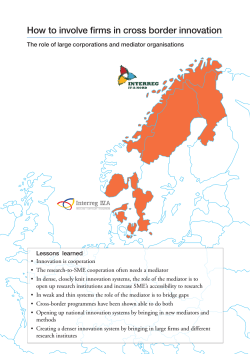


© Copyright 2026