
Why does child labour persist with declining poverty? NCER Working Paper Series
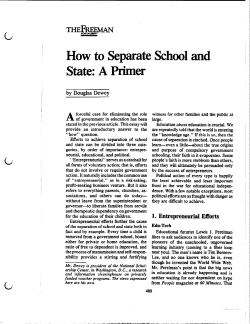
NCER Working Paper Series Why does child labour persist with declining poverty? Jayanta Sarkar Dipanwita Sarkar Working Paper #84(Revised) June 2012 Why does child labour persist with declining poverty? Jayanta Sarkara* a Dipanwita Sarkarb School of Economics and Finance b School of Economics and Finance Queensland University of Technology Queensland University of Technology 2 George Street, Z826 2 George Street, Z825 Brisbane, QLD 4000 Brisbane, QLD 4000 Australia Australia Email: [email protected] Email: [email protected] Abstract Uneven success of poverty-based approaches calls for a re-think of the causes behind persistent child labour in many developing societies. We develop a theoretical model to highlight the role of income inequality as a channel of persistence. The interplay between income inequality and investments in human capital gives rise to a non-convergent dynamic path of income distribution characterised by clustering of steady state relative incomes around local poles. The child labour trap thus generated is shown to preserve itself despite rising per capita income. In this context, we demonstrate that redistributive policies, such as public provision of education can alleviate the trap, while a ceteris paribus ban on child labour is likely to aggravate it. Key words: Child labor; Health; Human capital; Income inequality; Multiple equilibria. JEL classification: I1, J2, O1, O2. * Corresponding author. Tel.: +61 7 3138-4252; Fax: +61 7 3138-1500. 1. Introduction The Third Global Report released by the International Labour Office (2010) raises serious concerns over the achievement of the Millennium Development Goal (MDG) for the elimination of child labour. In fact, the persistence of child labour has been identified “as one of the biggest failures of development efforts”. Approximately 215 million children are still engaged globally in some form of employment. Worse still, the proportion of employed children increased from 26.4% to 28.4% in sub-Saharan Africa during 2004-2008. Over the same period, an alarming 20% increase in global child labour in the 15-17 age group indicate that the progress made so far has been uneven. Remarkably, this coincides with a steady decline in global poverty, including in the poorest regions of sub-Saharan Africa.1 This calls for a re-assessment of the conventional approach which relies on poverty reduction strategies. The idea developed herein provides an explanation of why in some societies child labour persists with general rise in per capita income. A substantial body of literature argues that the main cause of child labour is poverty.2 However, recent micro-evidence casts doubt on the poverty-based explanations. For instance, income has not been a significant determinant of child labour in Peru (Ray, 2000a), its role has been modest in Ghana (Canagarajah and Coulombe, 1997), and even positive in India (Swaminathan, 1998, Kambhampati and Rajan, 2005). Furthermore, land holding – a strong predictor of household income in developing countries – is found to be associated with increased working hours among children in northern India (Basu et al., 2010), Ghana and Pakistan (Bhalotra and Heady, 2003), Burkina Faso (Dumas, 2007) and rural Botswana (Mueller, 1984). In fact, the impact of income incentives has been found to be heterogeneous across poor families in Pakistan and Nicaragua (Rosati and Rossi, 2003), suggesting the importance of factors beyond absolute poverty. The macro-development literature points to income inequality as one of the 1 According to World Bank’s (PovcalNet) poverty estimates, Poverty Headcount Ratio and Poverty-Gap have fallen by approximately 9% in sub-Saharan Africa at the ‘poverty-line’ of $1.25/day. Relevant data are available at: http://iresearch.worldbank.org/PovcalNet/index.htm 2 Prominent contributions focus on the role of poverty in conjunction with other factors, such as capital market failure (Basu and Van, 1998; Basu, 1999), segmented labour markets (Behrman, 1999), breakdown of intergenerational contract (Baland and Robinson, 2000), nature of technological progress (Hazan and Berdugo, 2002) and endogenous evolution of preference structure (Chakraborty and Das, 2005a, 2005b). See Edmonds (2008) for a comprehensive survey. 1 ‘usual suspects’. The role of inequality has featured most prominently in the works of Ranjan (2001); Rogers and Swinnerton (2001), and Dessy and Vencatachellum (2003). Notwithstanding the insights provided by these studies, why child labour persists in growing economies remains to be understood. We provide a theoretical basis and numerical validation to highlight the critical role of income inequality as a channel of persistence under constant income growth.3 A preliminary look at cross-country data from the World Development Indicators in Figure 1 suggests a positive association between inequality and economic activity of children, irrespective of the level of per capita income. This regularity is borne out more clearly from micro-data on three developing countries from the Young Lives Survey – India, Ethiopia and Peru. Ranking the countries by inequality level using the Gini index followed by comparisons of child labour within and across the three in Table B.1 confirms the association in general and for the poorest 10% in particular (see Appendix B for results and a brief description). Thus the higher incidence of child labour in more unequal societies is likely to be observed among the poorest sections. In theory this can be overcome with rising income. However, the presence of health as an input in human capital can inhibit this escape. We formalise this argument below. The intuition behind the persistence mechanism rests on two premises. First, schooling entails a fixed cost. Second, health and skill are complementary inputs in human capital production, and both can be augmented via private investment.4 The first assumption implies formal education and hence skill is relatively expensive for the poor households inducing them to substitute health for education. These families therefore choose low schooling and high child labour. In the extreme case, schooling becomes zero if the degree of inequality is too high. Health-skill complementarity magnifies the human capital penalty (reward) due to forgone (additional) schooling among the poor (rich) families. The divergence of relative income and child schooling (labour) thus generated cannot be arrested by economic growth because of its 3 As is common in the literature, assuming income is a positive transformation of human capital, the terms ‘income’ and ‘human capital’ are used interchangeably. Income inequality, defined as the ratio of individual incomes to the mean, implies relative inequality as opposed to absolute inequality that depends on absolute difference in income. 4 Both are well-grounded in micro evidence. The presence of high schooling cost in developing countries have been well documented (see, for example, McEwan, 1999, Hazarika, 2001, Deininger, 2003) and formalised in the notion of ‘indivisibility’ of educational investment (Ljungqvist, 1993, Galor and Zeira, 1993). Likewise, health-skill complementarity is backed by compelling evidence, typically in the context of children (Almond and Currie, 2010, Heckman, 2007). 2 effect on the cost of schooling and return to health. A rise in average income simultaneously raises teachers’ wages and public investment in health. The former makes schooling more expensive for the poor, while the latter encourages private health investment. The two effects reinforce the intra-household substitution of health for schooling among the poor, thereby sustaining inequality and child labour. Thus the long run dynamic is characterised by polarisation of households into multiple steady states, including one that represents an intergenerational child labour-trap. Whether a family will be caught in the trap or not depends on its position in the initial income distribution. Our contribution to the literature is manifold. First, we underscore the independent roles of health and skill as two distinct components of human capital. . Health is indispensable lacking which marketable work is infeasible. Skill on the other hand, earns a higher return, but costs more to accumulate. One ramification is that health offers poor families an alternative route for human capital formation when formal schooling is too costly. As an important source of income, child labour can thus prove to be beneficial in the short-run. Second, health-skill complementarity along with differential access to schooling endogenously generate nonconvexity in human capital production leading to non-convergence of inequality. This mechanism is distinct from the credit market imperfection channel (Galor and Zeira, 1993), technological non-convexity (Galor and Tsiddon, 1997) and minimum health requirement (Ray and Streufert, 1993). Third, in line with Ranjan (2001) we incorporate child leisure time, a feature that gives rise to non-monotonic relationship between child’s employment hours and household income.5 Finally, we analyse persistence of child labour along a balanced growth path. Since perpetual growth in per capita income is likely to prevent the transmission of a child labour trap across generations, it is the weakest possible growth-related assumption that brings to the fore the role of relative-income dynamics instead of being subsumed by growth issues. The policy implications of the study are striking. A ceteris paribus ban on child labour – a popular recommendation aimed at raising school attendance – is likely to be unsuccessful and additionally to reduce household investment in child health, thereby aggravating the level of human capital at the low-level equilibrium. Instead, our results emphasise the need for redistributive policies that reduce the fixed cost of human capital for the poor, rather than 5 Swaminathan (1998), Kambhampati and Rajan (2005), and Fafchamps and Wahba (2006) provide empirical support to the non-monotonic relationship using data from India and Nepal. 3 conventional poverty reduction measures that leave the relative cost unchanged. In this context, we discuss how a child labour trap can be avoided in the long run through public provision of education which obviates the relative cost effect. A third policy implication arising from the calibrated version of the model suggests that the distance between the steady states can be reduced, or even eliminated, by raising the effectiveness of public and/or private spending on child health. For sufficiently high returns, private health investment raises future human capital stock beyond the critical level required for schooling. Therefore, public investment in improved health infrastructure may go a long way in eliminating a child labour trap. Numerical simulation results reveal that the dynamic trajectory of relative income is able to generate three steady states along the balanced growth path, capturing the possibilities of full, partial, and zero child labour. Of these, the partial scenario represents an interesting combination of schooling and market work among the richer-than-average households. This feature is distinct from the majority of poverty-trap models with a unique no-child labour high equilibrium. Existence of children in employment among the richer families ties well with the evidence in Bhalotra and Heady (2003), Rogers and Swinnerton (2004), and Basu et al. (2010) among others. The rest of the paper is organised as follows. Section 2 presents the set up of the model. Section 3 analyses the theoretical results, and discusses the role of health in intergenerational transmission of inequality and child labour. This section also discusses the quantitative aspects of the model through simulation of a calibrated version of the model. Section 4 discusses implications of the model in the context of two policy options to reduce child labour – free public provision of education and an explicit ban on child labour. Section 5 concludes. 2. The Model Consider a discrete time, infinite horizon overlapping generations economy populated with a continuum of individuals who live for two periods – childhood and adulthood. Individuals are heterogeneous with respect to their embodied skill. A household is a family unit consisting of a child and an adult (parent), each of whom is endowed with a unit time. Parents are altruistic – they derive positive utility from the child’s future human capital. A parent takes all economic decisions and optimally chooses the amount of consumption, ct, child’s schooling time, et, child’s labour time, lt, and nutritional and medical spending on child’s health, nt. Choice of et 4 and lt determine child’s leisure time, xt, as a residual. In this simple set-up, there is no uncertainty regarding returns to human capital. Household size can influence decisions regarding human capital investment and complicate the endogenous evolution of income distribution.6 To circumvent the influence of population growth on income distribution, population is assumed constant and number of children per household is normalised to unity. However, it is worth noting that the qualitative characteristics of the model remain intact even when fertility is an endogenous decision (see Appendix A). We extend the standard binary choice (schooling versus work) framework to include the possibility that children may neither attend school, nor participate in the labour market, and instead remain idle.7 In the child labour literature idleness among children has been ascribed to factors such as labour market frictions, low ability, poor health, importance of household work, etc. We interpret child idleness as conferring a positive non-economic benefit to parents as it involves helping with unpaid household work, and being available to care for the younger, ill and infirm family members. Since parents derive utility from child ‘idleness’ it is akin to ‘leisure’ from the modelling perspective, and we use these terms interchangeably.8 Denoting child leisure by xt, the time available for work is (1 – et – xt) for a child. The utility function of an adult parent is given by: ln ct ln( xt ) ln Ht 1 (1) The parameter β > 0 represents the psychological discount factor and H t 1 denotes the effective human capital of her child upon reaching adulthood. The parameter ν > 0 represents the weight parents put on child leisure relative to consumption, ct, and δ > 0 is a constant. Departing from the existing literature we conceptualise ‘health’ and ‘skill’ as two endogenous and complementary components of human capital. Health status positively affects returns to skill by reducing morbidity and increasing the productivity of labour time. Higher 6 For example, Chakraborty and Das (2005b) establish a positive link between fertility and child labour. Distributional issues, however, were not analysed. 7 A number of studies find evidence of child idleness. Ravallion and Wodon (2000) find 54% of children in Bangladesh while Rosati and Tzannatos (2000) report 2.2 % – 3% children in Vietnam neither work nor attend school. Deb and Rosati (2002) estimate that idle children constitute 14% in Ghana and 23% in India. 8 See Brezis (2010) for an explanation why parents may care more about child leisure than child consumption. 5 skill, on the other hand, raises the effectiveness of labour. We assume a simple multiplicative form to capture the complementarity between health and skill ‘inputs’ in the production of human capital: Ht 1 ht 1st 1 (2) where ht 1 denotes the health-status of an adult with skill level st+1.9 A child’s future (adulthood) health can be improved by undertaking health investments, nt, in childhood. We think of health investments as consisting of expenditure on nutritional food, safe drinking water and sanitation, vaccination against preventive diseases, medical care, healthy activities, etc. Following Schultz (2009) we assume that future health also depends on the quality of health infrastructure, such as water, sanitation, community disease control programs, etc. Quality of health infrastructure in period t+1 is assumed to depend on the level of government health spending in the previous period (Gt).10 Apart from direct spending, future health of a child is determined by her ‘initial endowment’ derived from parent’s human capital, Ht. Not only does a child genetically inherit her parent’s health, but the influence of parental education is almost unanimously agreed upon in the empirical literature.11 We assume a simple constant returns to scale technology for health, with each input exhibiting diminishing returns12: ht 1 nt Gt Ht1 , > 0, 0 , 1 (3) The skill level of an adult at time t+1 increases with the time spent in school as a child, et, but at a diminishing rate: st 1 ( et ) , > 0, 0 ≤ et ≤ 1, > 0, 0 < η < 1 (4) Note that skill level is positive even when schooling time is zero. This can be interpreted as the ‘autonomous’ level of skill resulting from positive interactions at the household and social levels. and represent total productivity parameters in the accumulation of health and skill, respectively. The budget constraint for an adult with human capital Ht is: 9 The increasing returns to scale property of the human capital production function is purely for simplicity. Our analytical results are robust to alternative specifications, such as constant returns to scale. See section 3.2. 10 Complementarity between private and public health inputs have been used in Bhattacharya and Qiao (2007). 11 See Charmarbagwala et al. (2004) for an excellent survey. 12 Schultz (2009) provides supporting evidence for the diminishing returns properties. The constant returns to scale property ensures a balanced growth equilibrium. 6 ct nt et wt Ht (1 )wt Ht (1 et xt ) wt Ht (5) where wt is the wage per unit of human capital and (0,1) is the proportional income tax rate. A child is assumed to possess a fraction of the adult human capital, so the second term on the right hand side of (5) denotes earning from time spent as child labour. The cost of human capital formation is dependent on the prices of schooling and health inputs. While price of health inputs is the same as that of consumption goods, price of schooling is higher than that of consumption goods among the poor. In practice direct cost of schooling can impose significant burden on the poor. For example, McEwan (1999) suggests that private direct costs exceed 20% of the total cost of education. Tilak (1996) argues that households in India spend a substantial part of family income paying various forms of fees (tuition, examination and other) even in public primary schools. Hazarika (2001) and Deininger (2003) present evidence from Pakistan and Uganda, respectively, on direct costs discouraging schooling. Momota (2008) argues that private costs of schooling, such as outlays for school materials, transportation, etc., are often indivisible and form a substantial part of schooling costs and impose a large burden on the poor even in a ‘free’ education system. These suggest schooling costs may be higher for households in the lower rung of the income strata.13 Following Dahan and Tsiddon (1998) and de La Croix and Doepke (2003), a simple yet effective way to introduce this feature is to assume teachers possess the average human capital in the population H t , implying a schooling cost of et wt H t per child. In the absence of a credit market, the cost barrier is higher the poorer the household.14 Investment in child health via nutritional goods, nt , on the other hand, is assumed to cost the same as the final consumption good. 13 Tilak (2002) concludes that households from even lower socio-economic and occupational background spend considerable amounts on acquiring education, including elementary education, which is expected to be provided by the State free to all. The Public Report on Basic Education in India (PROBE, 1999) finds that schooling costs are substantial, especially in northern states of India: “In fact, ‘schooling is too expensive’ came first (just ahead of the need for child labour) among the reasons cited by PROBE respondents to explain why a child had never been to school” (p. 32). 14 As will be clear in the next section, all results remain valid when the fixed cost of schooling is an increasing function of H t . 7 A representative firm produces the consumption (and nutrition) goods using a production process with labour as the only input: Yt ALt , A > 0 (6) where Lt is the aggregate labour supply. The firm chooses inputs by maximizing profits Yt – wtLt. Therefore, the competitive wage rate per efficiency unit of labour is given by wt = A. The initial old are assumed to differ only with respect to skill, s0, with an initial distribution M 0 ( s0 ) . At any time t skill is distributed over the adult population according to the distribution function Mt(st). The average skill level st is given by st st dM t ( st ) . The stock of 0 human capital Ht ( ht st ) has the distribution function Ft ( Ht ) M t Ht ht ,where ht is presumably a function of individual state st. The average human capital H t is: H t H t dFt ( H t ) (7) 0 Assuming total population is constant and normalised to unity, the stock of human capital evolves according to: Ft+1( H ) = I ( H t 1 H ) dFt ( H t ) (8) 0 where I (∙) is an indicator function. The market clearing condition for labour is: 0 0 0 Lt H t dFt ( H t ) et H t dFt ( H t ) (1 et xt ) H t dFt ( H t ) (9) The condition implies child labour adds to the total supply of labour, while time devoted to teaching is unavailable for production of the consumption good. We define an equilibrium for our economy as follows: Definition 1: Given an initial distribution of skill M 0 ( s0 ) an equilibrium consists of sequences of aggregate quantities {Lt, H t }, distributions Ft 1 ( H t 1 ) , and decision rules {ct, nt, xt, lt, ht+1, st+1} such that (i) the households’ decision rules ct, nt, xt, lt, ht+1, st+1 maximise utility (1) subject to budget constraint (5); (ii) the firm’s choice of Lt maximises profits; (iii) the price wt is such that the labour market clears; (iv) the distribution of human capital evolves according to (8); (v) aggregate variables { H t , Lt} are given by (7) and (9). 8 3. Theoretical Results We begin the analysis by characterising the optimal household choices of schooling, child labour, and health investment. We find both schooling and health investment increases, and idleness decreases with relative income. Families below a threshold level of relative income choose zero schooling and full time child labour. Child labour is found to have a non-linear relationship with income: it increases with income so long as schooling is zero, and falls thereafter. Using interior decision rules we derive the dynamic path of individual human capital along a balanced growth path. Finally, we examine its long run properties using a calibrated version of the model. 3.1 Education, Child Labour and Private Health Investment We find that individual household decisions depend on the dispersion of human capital. The household decisions are obtained by maximizing (1) subject to (2) – (5). We express the optimal household decisions in terms of a key variable zt Ht Ht ht st ht st , human capital Ht of a household relative to the average human capital H t of the society. For households who meet the conditions for interior solutions, the first order conditions imply: et 1 zt 2 , 3 (1 zt ) (10) nt Ht 1 zt 2 (11) m1 m2 zt (12) xt where, 1 (1 (1 )) (1 ) , 2 (1 ) , 3 1 ( ) ,15 1 A (1 (1 ) 3 , 2 A / 3 , m1 (3 ) , m2 (1 (1 ) ) (1 ( )) (3 ) . Given (10) and (12), a child’s time at work is given by: l ( zt ) 1 e( zt ) x( zt ) , or 15 A large enough value of of the return to schooling, , ensures 1 > 0. In particular, this holds for (1 ) (1 (1 ) 9 lt 1 1 zt 2 m1 m2 3 (1 zt ) zt (13) Note from (13) that the possibility of the event {lt = 0, et = 1} is guaranteed if m2 < 0 – a parametric restriction we will impose for the rest of the paper. Note also that, xt 0, as zt m1 m2 . Given the decision rules in (10) and (11), and denoting , the human capital of a child in period t+1 is given by: H t 1 ht 1st 1 1 zt 2 z 2 1 (Ht ) 1 t Gt ( H t ) (1 z ) 3 t (14) The individual decision rules in (10) – (13) merit some discussion. Equation (10) suggests that optimal choice of schooling time is increasing and concave in relative human capital ( det dzt 0, d 2et dz t2 0 ). More importantly, schooling is zero if the relative human capital is below a critical level ze ( 2 1 ). This implies, families with relative human capital zt ze , will be fully engaged in child labour. The further below one is from the average in human capital distribution, the higher is the burden of schooling due to two reasons – (i) cost of schooling is determined by the average human capital, and (ii) opportunity cost of schooling in terms of foregone income from child labour. The fact that schooling is a concave function of relative human capital has important implications. It implies that the average quantity of schooling in the society depends upon the dispersion in the distribution of skill. In particular, if the dispersion of skill increases for a given average skill level, by Jensen’s inequality the concavity in the schooling function implies that the average schooling in the society will decrease. Therefore, higher inequality in skill distribution would lead to a lower average skill level, st 1 and a higher average quantity of child labour and leisure. The fact that health status is also a concave function of relative human capital, as discussed below, amplifies the negative effect of inequality on aggregate skill accumulation. Differentiation of lt in (13) reveals an inverted-U relationship with relative income. As seen from (12), idleness declines with relative income as families equate its marginal utility with the opportunity cost of foregone child labour net of returns from schooling. Hence idleness falls and child labour rises with relative income, until the threshold level of zt required for positive schooling is reached, whereafter child labour declines yielding an inverted-U. The positive part of this relationship is consistent with empirical evidence. For example, Swaminathan (1998) 10 documents economic growth raises children’s wage employment in Gujarat, India. Kambhampati and Rajan (2005) report similar findings across Indian states. Figure 2 plots children’s time spent in school, leisure and work as a function of parental relative income. The nature of health investment is quite distinct from that of educational investment. Note from (11) that demand for nutrition or health inputs (nt) is linear in zt ( dnt dzt 0 ) with a positive intercept. This implies there exists an autonomous, subsistence-level consumption of health inputs. Nutrition acts an essential input in the health production function. Unlike education, health investment rises with the average level of human capital in the economy for all households. In other words, health status in our model is positively associated with economic growth, which is consistent with the findings in the empirical growth literature. This result follows from the substitution effect – as H rises, relative price of education rises, inducing all families to substitute health for education. Finally, from (3) and (11), it is clear that like skill, health status is a concave function of relative human capital. 3.1.1 Corner solutions A key feature of this model is the possibility of multiple corner solutions. As discussed above, the fixed direct cost of schooling prevents households with zt < ze from accessing education. Full time child labour is an optimal choice for these households. The relevant first order conditions imply: et = 0, (15) nt 3 H t , where 3 xt A (1 (1 )) 1 (1 ) (1 ) (1 ) (16) (17) Given that investment is made in health only, the human capital of a child in period t+1 is: Ht 1 ht 1st 1 3 Gt ( Ht )1 . Absence of schooling makes the demand for health inputs independent of H , and leisuretime constant. A parent spends a fraction of her income on child health, which sustains the child’s human capital in adulthood. 11 Given that schooling is an increasing and leisure is a decreasing function of zt, and that time endowment is bounded in [0, 1], the possibility of two more corner cases arise: lt = 0 and xt = 0. Which corner obtains first as zt increases? Denote zt = z x such that x( z x ) = 0, and zt = zl such that l ( zl ) = 0. Also denote zt = ze such that e( ze ) = 1. From (12) z x = – m1/m2, and from (10), ze ( 2 3 ) (1 3 ) . It can be shown that zl ze , if the parametric restriction ( 2 3 ) (1 3 ) m1 m2 holds. While this restriction is not crucial for the qualitative results, in the numerical version of the model, we do impose this discipline on parameter values. Intuitively this implies z x zl ze , as depicted in Figure 2. Maximisation problem at this corner implies the following decision rules: et = 1 (18) nt (4 zt 5 ) Ht , (19) where 4 A (1 ) (1 ) , and 5 4 (1 ) . At this corner, the human capital of a child in period t+1 is: Ht 1 ht 1st 1 (1 ) 4 zt 5 ( Ht ) Gt ( Ht )1 . 3.2 Dynamics of Individual Human Capital Given that the stock of human capital is distributed as Ft( H t ), the distribution of relative human capital levels can be expressed as t ( zt ) Ft ( zt Ht ) . Given constant population, the evolution of t ( zt ) occurs according to: t 1 ( z ) I ( zt 1 z ) d t ( zt ) (20) 0 Given the definition of z, it must be that 1 zt d t ( zt ) (21) 0 Decisions on child’s schooling and health are given by (15) and (16) if 0 zt ze , by (10) and (11) if ze zt ze , and by (18) and (19) if zt ze . Future skill-level of children is given by: z 2 st 1 max 0, min 1 t ,1 (1 z ) 3 t 12 (22) From (9), equilibrium labour input is given by: ze Lt H t zt d t ( zt ) e( zt ) d t ( zt ) 1 e( zt ) x( zt ) zt d t ( zt ) which leads to ze 0 0 Lt 1 1 (1 m1 m2 ) ( 2 1 ) Ht 3 (23) Using (6) and (23), income per unit of labour hour in equilibrium is: Yt 1 AH t 1 (1 m1 m2 ) ( 2 1 ) Lt 3 (24) Public provision of health infrastructure is funded by income tax on adults. Assuming the government maintains a balanced budget every period: Gt wt H t dFt ( H t ) AH t (25) 0 Substituting (25) in (14), we obtain the following dynamic path of human capital when investments in both schooling and health are non-zero: H t 1 ( A) 1 zt 2 1 zt 2 1 ( H t ) . The following equation (Ht ) (1 z ) 3 t represents this path for all ranges of zt. 1 ( zt )1 H t , if zt ze z 2 1 H t 1 2 1 zt 2 1 t H t , if ze zt ze ( zt ) (1 z ) 3 t 1 Ht , otherwise 3 4 zt 5 ( zt ) (26) where, 1 ( A) 3 , 2 1 / ( 3 ) , and 3 ( A) (1 ) . Using the definition of z and (26) and noting gt+1 = H t 1 H t , the relative human capital for an individual in t+1 is given by: 1 gt11 ( zt )1 , if zt ze 1 zt 2 1 1 zt 1 2 gt 1 1 zt 2 , if ze zt ze ( zt ) 3 (1 zt ) 1 1 , otherwise 3 gt 1 4 zt 5 ( zt ) 13 (27) 3.2.1 Evolution of income inequality under balanced growth path Note that the dynamic system described above is block recursive. Given the initial conditions, we first solve for et and nt using (10), (11), (15), (16), (18) and (19). Then using (21) and substituting the optimal values of et, nt and Gt (from (25)) in (27) we determine zt+1 and corresponding gt+1. The value of zt+1 thus obtained is then substituted in (21) led one period ahead. This yields an expression of gt+1 as a function of current variable zt. The new distribution of relative human capital is given by (20). Ht+1 is non-negative, which ensures that an equilibrium exists for any given initial conditions. We analyse the evolution of relative human capital assuming a balanced growth path (BGP) for the economy, along which the growth rate of output (and that of H) is constant. This implies gt = g*. The BGP assumption helps us analyse the dynamic path of individual relative human capital without deviating to growth issues. Along a BGP the economy is characterised by a long run scenario of perfect equality – that is, H t H t for all adults. Therefore, such a path is characterised by d(1) =1 (i.e. the limiting distribution is degenerate) for zt 0 . Note that this is satisfied uniquely for the range ze zt ze as this range includes z = 1, where d(1) =1 holds. Therefore, the balanced growth rate of output and human capital correspond with the intermediate range ze zt ze , and is given by: g* 2 1 2 1 2 3 (1 ) (28) The value of g* in (28), the evolution of the relative human capital in (27) can now be written as: 1 g *1 ( zt )1 , if zt ze 1 zt 2 1 1 zt 1 2 g * 1 zt 2 , if ze zt ze ( zt ) (1 z ) 3 t 1 1 , otherwise 3 g * 4 zt 5 ( zt ) (29) Given e(z = 1) ≤ 1, that is, 1 2 3 (1 ) , it is immediately verified that z* = 0 and z* =1 are solutions to the difference equations in (29). The solution z* = 0 is trivial, while the steady state at z* = 1 corresponds to a degenerate distribution whereby individual differences in human capital cease to exist and the economy attains perfect equality. 14 3.2.2 Multiple steady states Let us now examine (29) more closely with the help of Figure 3. For the range zt ze , the dynamic path of relative income is given by zt 1 (1/ g*) zt1 , an increasing and concave * relationship in [0, z F ] as shown in Figure 3. In this range characterised by no schooling, a child’s time is allocated between market work and leisure (we denote this outcome as full child labour). The corresponding steady state z F* (F stands for full) is stable, as the curve intersects the 45 degree line from above (point ‘a’). For families at this steady state human capital is propagated across generations solely through health investment. As relative income attains a value ze , investment in education kicks in, inserting a discontinuity in the zt+1 trajectory. It is straightforward to show dzt 1 dzt |zt ze , ze zt ze dzt 1 dzt |zt ze , implying a steepening of the trajectory at the beginning of the range ze zt ze . Given the BGP assumption discussed above, the curve must intersect the 45 degree line at z* = 1, which corresponds to point ‘b’ in Figure 3. As our numerical simulations discussed in section 3.3 reveal, the trajectory intersects the 45 degree line from below at ‘b’. So it represents an unstable steady state. The concavity of zt+1 produces another * intersection with the 45 degree line at z P (point ‘c’) which represents a high-level, stable * equilibrium. Note that with the parametric restriction for zl ze , z P (P stands for partial) does not coincide with the corner solution {et = 1, lt = 0}. Partial child employment exists among the households converging to this steady state. This feature, though not in conformity with the ‘luxury axiom’ of Basu and Van (1998), has found empirical support in Pakistani and Peruvian data (Ray, 2000b). Finally, as relative income reaches ze , households invest in full time schooling, inducing an upward shift in the trajectory given by zt 1 3 g *1 4 zt 5 ( zt )1 . The magnitude of the shift depends on the parameter values. Note that, like the previous two segments, this part in [ ze , ∞) is also increasing and concave in zt. Yet another intersection with the 45 degree line * from above, yields a third, stable and super steady state of no child labour at z N (N stands for * no) denoted by point ‘d’ in Figure 3. Thus, z N is characterised by {et = 1, xt = lt = 0}. 15 Points ‘a’, ‘c’ and ‘d’ are local poles the location of which depend on the parameter values. Which pole the households will be attracted to, however, depends on their initial position in the relative income ladder. Households with z0 1 will gravitate towards the low-level * equilibrium, z F , while the others will be attracted towards the two high-level equilibria. * Specifically, households with 1 z0 ze will cluster at z P , while those with z0 ze will * * converge to the super equilibrium z N . Typically, given the small mass at z N , the resulting distribution of individual human capital in the long run will look like the one shown in Figure 5. * Those at steady state z F will find themselves trapped in a vicious cycle of high morbidity and high child labour. Remark 1: The critical role played by health investment in the above process is worth emphasising. Note that the fixed schooling cost that generates a threshold-effect in educational investment is able to produce rich-poor difference in human capital accumulation. But skill as the sole component of human capital may not be sufficient to produce multiple steady states under endogenous growth. In general, the long run distribution of individual relative income is likely to be degenerate if human capital is one-dimensional and is subject to diminishing returns. This is confirmed by a calibration-simulation exercise similar to the one in section 3.3.16 The presence of health as a crucial twin component creates strong divergent forces in human capital formation that generate sufficient non-linearity in human capital production allowing for multiple equilibria. Remark 2: The multiplicity of steady-states is not due to the increasing returns to scale assumption in human capital production in (2). The results are valid with a more general specification of st+1 and Ht+1. Let Ht 1 ht1st1 (0 , 1) . In addition, let the schooling productivity ( ) depend on the existing school-quality, which is approximated by the level of average human capital of the society. Using a simple linear form for the productivity variable, such as t H t , (4) is rewritten as st 1 Ht ( et ) , > 0. Since households take H t as 16 We refrain from reporting the results of this exercise for the sake of brevity, but they are available upon request. 16 given, the decision rules (10) and (11) remain unaffected. In the interior range ze zt ze the period t+1 human capital is thus given by: H t 1 ht 1st1 1 zt 2 ( H t ) 1 zt 2 (1 ) . Gt ( H t ) 3 (1 zt ) Balanced growth equilibrium requires 1 , which leads to: ( A) zt 1 1 zt 2 gt 1 1 zt 2 3 (1 zt ) (1 ) ( zt ) (1 ) , if ze zt ze (27a) It is readily seen that in the range ze zt ze the dynamic properties of (27) and (27a) are identical. We prefer the simpler, more parsimonious specification. Further analytical investigation is cumbersome due to the complex non-linear nature of zt+1 in (29), especially for the range ze zt ze . Therefore, we resort to calibration and simulation of the model. In the next section we analyse a parameterised version of the dynamic path of relative human capital to examine the possibility of multiple steady states. 3.3. Computational Exercise The purpose of this exercise is to gain a better perspective of the dynamic evolution of income inequality and study the possibility and nature of the steady state equilibria. By simulating the model with meaningful parameter values we will be able to quantify the degree of polarisation of income distribution, and find the values of child labour, morbidity and other variables for different income groups at the steady states. 3.3.1 Parameter values Non-availability of adequate data on developing countries makes parameterisation of the model a difficult exercise. Therefore, wherever available, the parameter values, presented in Table 1, are selected to match the values for a typical developing country, and some are borrowed from the existing literature. The results of this computational exercise therefore should only be taken as qualitative description of a developing economy. As is standard in the literature, we assume that one model period (or generation) corresponds to 30 years. The wage of a child in efficiency units is assumed to vary in proportion to her parent’s wage. The parameter , representing the fraction of her parent’s efficiency wage 17 earned by a child worker, is assigned a value of 0.2. In other words, a child is assumed to earn about one-fifth of her parent. The period discount factor β is given a value of 0.95 to reflect an annual discount rate of 0.02%, which is in line with existing business cycle literature. The returns to schooling, is given a value 0.67, high enough to ensure 1 > 0. This value of , together with the value of total productivity parameter in skill function, = 2.15, imply H = H =1 in the degenerate equilibrium. Given = 2.15, the values of the total productivity parameters in output and health productions are pinned down by the value of g* in (28). This yields A =10 and = 1.16. The literature provides no guidance for the value of elasticity of health with respect to private health investment ( ) in the model. We choose = 0.3 which ensures that about 20% of household income is spent on health and nutritional goods at the lower steady state – a value that falls in the range found in the literature (Fabricant et al., 1999). Following de La Croix and Doepke (2003) we choose = 0.01. The value of the elasticity of leisure, and the shift factor, are chosen to reflect that the aforementioned parametric restriction that ensures child labour goes to zero before child leisure does (or, ( 2 3 ) (1 3 ) m1 m2 0 ). Specifically, we choose = 0.2 and = 0.6. In the model, individuals do not internalise the income tax, and a higher tax rate reduces schooling and health spending. Since, most of the population pays minimal taxes (if any), the average tax rate is assumed to be 5%, a conservative value. The value of the elasticity of health with respect to public health spending, , is a key parameter in the model as it largely determines the position of the equilibria in the long run. We choose a value = 0.45 to ensure that the ‘distance’ between the two steady state equilibria is not too large. We further analyse scenarios to test the sensitivity of the model to changes in these parameters. In addition to choosing parameters, we also need to set the initial conditions for income distribution. As mentioned in section 2, the overall size of the population is set to one, a scale parameter which does not affect the results. The initial distribution of human capital follows a standard log-normal distribution F ( , 2 ) , where the mean ( ) equals 0 and variance ( 2 ) equals 1. 3.3.2 Quantifying the multiple equilibria Given (29), the parameterisation discussed above produces a transition path of relative income as 18 shown in Figure 4. The simulated trajectory for entire range of z is not clearly visible in a single diagram – hence the steady states have been reproduced in panels A, B and C. As we intuitively argued in relation to Figure 3, the simulated trajectory of zt+1 intersects the line of equality at four points, z F* , zm* , z P* and z *N – only one of which ( zm* ) is unstable. The quantitative properties of the trajectories in panels (A) – (C) as depicted in Figure 4 are retained for a wide range of parameter values. Given the chosen values of parameters, the threshold values are given by ze = 0.018 and ze = 5.61. Table 2 provides the values of the key variables. The poorer households converge to z F* = 0.007 – the low-level equilibrium where individual human capital is about 0.07% of the mean. At z F* there is no schooling (given z F* < ze = 0.018), with 75% of a child’s time is spent at work and 25% at leisure.17 The health status of 0.07 reflects that health of a person at this equilibrium is about 0.7% of the average person in the society who has a health status of unity (alternatively, a person has a 93% higher morbidity than the average person). Skill level at this steady state is at 10% of the average. In terms of income and spending, health inputs account for about 22% of household income for these households. A child contributes about 14% of household income at this equilibrium. In contrast, at the higher steady state z P* , a typical individual has 5.245 times more human capital than the average person. Children in these households spend 97% of their time at school and the rest 3% at work. Child labour among the rich is inconsistent with the ‘luxury axiom’ of Basu and Van (1998), but Ray (2000b) found empirical evidence using Pakistani and Peruvian data that support our results.18 They have about 2.5 times better health, and 2.12 times higher skill level, than an average individual. Roughly 15% of household income is spent on health and 16% on schooling. 17 Since each family has one child, this can be interpreted as 75% of all children working full time, with 25% neither working nor attending school. 18 It is not hard to argue that in developing countries, even the richer families engage their children in family business and other work mainly as apprentice, in early preparation for a suitable occupation. 19 The super steady state is at z *N = 6.356 , and characterised by full time schooling for children (given z *N > ze = 5.61). Given their highest rank in the socio-economic status, households at this equilibrium outperform the others in all respects, as shown in Table 2. The balanced growth rate is found to be 0.3%, implying a slow, but steady growth of per capita income. Thus without policy interventions, the conditions at the three steady states would perpetuate in the long run despite income growth. Therefore, the economy in the long run is characterised by an inequality-child-labour-trap, with simultaneous presence of high morbidity and child labour on one hand, and excess investment in human capital on the other. 3.3.3 Polarisation For simplicity, and without loss of generality, we ignore the super steady state z *N in our remaining discussion. Figure 5 shows the history-dependence of the evolution of the distribution of relative human capital. Given initial distribution 0 ( z0 ) , the dynasties diverge to a tri-modal distribution ( z ) in the long run. Households with initial relative human capital zi < 1, converge to a distribution centred around z F* and those with zi >1, to a distribution around z P* . The level z = 1 acts as a threshold, determining the degree of persistence of intergenerational outcomes of human capital. The degree of polarisation or the distance between z F* and z P* is however a function of values of certain model parameters. The relationship is represented in Table 3, notable among which are those with , , and . A rise in labour productivity of children, , lowers the degree of polarisation, as does a rise in the elasticity of health production with respect to public health spending, . Higher labour productivity of children raises family income of the poor group and their relative human capital via improved health. The health elasticities of private spending ( ) and government spending ( ) raise health for both rich and poor, but in the absence of schooling, the marginal benefit for the poor is larger. As expected, a higher return to education raises the benefit of schooling for the rich, and this increases the distance between the two steady states. Income tax in this model has a redistributive effect through health accumulation. Therefore, an increase in the tax rate, τ, while reducing the incentive to educate and spend on health by all individuals, reduces the degree of polarisation. 20 These results suggest a key role for public health. An efficient health infrastructure not only raises the returns to private health spending, but also plays a crucial role in reducing the rich-poor gap in societies with high income inequality. In fact, the dynamic trajectory of zt+1 is quite sensitive to changes in , and it can be shown that the economy will be able to escape the inequality-trap if is increased from 0.45 to 0.6. 4. Discussion: Policy options to combat child labour In most societies child labour is discouraged through a host of policy measures ranging from outright ban to incentive-based schemes, such as conditional cash transfers. The success of these policies has been uneven, especially in societies where child labour is deep-rooted. One possible reason is that these policies are based on the premise that all poor face the same disincentive (incentive) for schooling (child labour). The model discussed here calls for more nuanced policy measures that recognise heterogeneity among households under poverty. For example, conditional cash transfers may raise schooling in a healthier family closer to the poverty line, but not in a poorer family with poorer health, simply because the latter simply may not perceive a positive net benefit from schooling, due to indivisibility of costs associated with attending schools. These costs often impose a larger burden on the poor, as discussed earlier. The results indicate that if schooling is too costly, child labour may in fact be beneficial for the poor since income from children supports investment in their health. Thus, it is possible that an outright ban on child labour would worsen poverty and child health by eliminating child income. This scenario is discussed in section 4.2. In many societies policy makers typically assume economic growth will trickle down to the bottom, reducing poverty and child labour. Our results imply this process will raise child income and encourage child labour, unless income inequality is reduced as well. Some income redistribution occur in our model through provision of tax-financed public health, but as we demonstrate below, redistributive policies in education, such as provision of free education, are needed to reduce income inequality and child labour. 4.1. Provision of Public Education A majority of developing countries have a highly subsidised public education program in place, aimed at lowering the direct cost of education to make it more affordable. Our model suggests that even with free public education, the society may find some child labour to be optimal. In the 21 modified model with free public education, households maximise (1) subject to the budget constraint ct nt (1 ) Ht (1 et xt ) wt Ht . For households who meet the conditions for interior solution, the first order conditions imply: 1 (1 ) (1 ) , 1 ( ) et e nt 6 H t , xt x (30) (31) (1 ) (1 ) ( ) 1 ( ) (32) where wt = A, and 6 A 1 (1 ) [1 ( )]1 The second order conditions for a maximum are satisfied. Note that each parent will be identically inclined to send their children to work if 0 < e x < 1. The children, in turn, will possess identical amounts of gross human capital. Now that the government has the twin responsibility of financing education as well as public health, operating under a balanced budget condition entails: Total tax revenue = Salary of teachers ( Gte ) + spending on health infrastructure ( Gth ) or, wt H t ewt H t ( e ) wt H t Gte Gth The accumulation function for human capital is now given by: Ht 1 (( e ) A) 6 Ht1 Ht e The dynamic of inequality in this regime will be governed entirely by the evolution of health status of agents. The relative human capital of children can therefore be written as: zt 1 ( g )1 (( e ) A) 6 zt1 e (33) where g (( e ) A) 6 e is the implied balanced growth rate. Note that under this policy regime, public health infrastructure is absent and Ht+1 = 0, unless e . There is a clear trade-off between public investment in health and education. Under this regime, the government has to raise the tax rate enough to finance both education and health.19 However a higher τ makes the inequality 0 e 1 more likely to hold, implying that in an interior equilibrium 19 See Sarkar and Osang (2008) for a similar analysis. 22 child labour will always exist in all households. As is clear from (33) the transition path of income inequality is increasing and concave for zt > 0, implying a unique and stable steady state as shown in Figure 6. Hence, provision of public education corresponds to perfect equality in the long run. However, in practice public provision of good quality schooling for the masses may not be feasible in the short run. While it is desirable for the children to be only in the school, schooling combined with employment may be a more realistic alternative. In fact, it may even be a preferred option as the presence of a non-corner high-level equilibrium ( z P* ) in our simulation exercise indicates. Peruvian evidence in Ray (2000a) suggests that many children combine schooling with employment. Many of these children will not be in schools if they were also not working. Therefore, a possible short term policy would be to allow more night-time schooling while letting children work during the day. In the long run, proper redistributive policies can be pursued to pull every child to full time schooling. A strong disincentive for schooling may also arise among the poor due to ‘perceived’ returns to education even when schooling is ‘free’. They may believe the skills acquired from school are not going to be ‘useful’ for the type of low-skill jobs their children will find as adults. This effect is compounded in highly unequal societies, where the quality of publicly provided schools is usually abysmal. This acts as a further disincentive (incentive) for parents to send their children to school (work). There is some evidence, for example, in Ray (2003), that this is indeed the case. Therefore, improvement of school quality will be effective in raising schooling incentive if the information on benefits of schooling is properly disseminated among the poor. Next we discuss a popular policy option that has been attempted in many poor countries – a ban on child labour. Our objective is not to claim child labour ban is linked with income inequality, but rather to examine the implication of this policy for our model, and to analyse its effects on the children’s outcome. 4.2. Ban on Child Labour We show that in a society where a large segment of the population does not have much access to education and health inputs, a ban would be undesirable. Given everything else, a ban on child labour would further reduce household earnings and end up hurting the poor. 23 In our model, a ban on child labour can be interpreted as forcing the child wage to zero. Under the ban, the relevant budget constraint is ct nt (1 )wt Ht et wt Ht , along with the time restriction et + xt = 1. The first order conditions for this problem are: et wt H t ct xt (34) 1 ct nt (35) In equilibrium, the net marginal benefit for one hour of schooling (left hand side of (34)) should be equal to the marginal cost of foregone consumption and leisure (right hand side of (34)). The ban eliminates the opportunity cost of schooling, but a closer look at (34) reveals that a distortionary effect in the choice of leisure appears if we assume schooling is a normal good – that is, an increase (decrease) in human capital raises (lowers) schooling. However, a rise in human capital results in a rise (fall) in schooling expenditure (ew H ) as well, which prevents consumption from rising (falling) much. Hence leisure must rise (fall) for (34) to hold. That the time constraint does not allow both schooling and leisure to increase simultaneously creates a distortion and sub-optimality. Therefore a ban will either make schooling an inferior good, or reduce lifetime expected utility of the households through sub-optimal choices. Another aspect of a ban is its negative effect on the household budget and resulting reduction in the affordability of health and nutrition. The health investment decision in (35) yields nt wt (1 ) (1 ) Ht et Ht , which implies health inputs and positive future human capital are unaffordable for parents with Ht et Ht (1 ) . A ban on child labour thus either distorts the schooling-leisure choice or makes schooling an inferior good. Furthermore, it reduces family income and optimal health investment. Given the health-skill complementarity this leads to reduction in optimal schooling, with a higher number of households choosing zero health and schooling for their children than under no ban. Thus a society as a whole, is likely to be worse off under the ban. 5. Concluding Remarks The objective of the paper is to explain the persistence of child labour despite rising income as observed in a number of developing countries. We highlight the role of income 24 inequality as a channel for transmission of child labour. When health and skill both matter in human capital production, income inequality sustains itself despite constant income growth. In this process, high schooling cost generates child labour while health plays a critical role in perpetuating the rich-poor divergence in human capital. The policy implications that follow are important. First, we show that a ban on child labour could be counterproductive to the intended improvement in child education and welfare. It would only distort the schooling-leisure choice and result in lower health, lower schooling and increased idleness among children in poverty. Second, free public education, a well-understood redistributive policy that encourages schooling, raises schooling, lowers morbidity and reduces income inequality in the long run. In practice, however, school quality is a critical determinant of schooling incentives among the poor that remains unaddressed. For example, a schooling subsidy to the poor will have little impact on a child’s time allocation unless the school quality is high enough to ensure a perceptible difference in the child’s outcome. Third, as indicated by the calibration results, raising productivity of public health infrastructure could confer similar benefits as public education, and additionally may even eliminate child labour. A child health policy has not yet been recognised as a tool in the fight against child labour. Some progress has been made in assessing the impact of child labour on future health, but the relationship between the quality of community health and the incidence of child labour is yet to be thoroughly investigated. These offer promising avenues of future research. Acknowledgements The paper benefitted from discussions with Ranjan Ray and Pushkar Maitra. The authors also thank Richard Barnett, Uwe Dulleck, Paul Frijters, Lionel Page, and the seminar participants of Queensland University of Technology, University of Queensland and the 7th Annual Conference on Economic Growth and Development at the Indian Statistical Institute, New Delhi, for helpful comments. All remaining errors are, of course, ours. 25 References: Almond, D., Currie, J., 2010. Human Capital Development Before Age Five, NBERWorking Papers No. 15827. Baland, J.M., Robinson, J.A., 2000. Is child labor inefficient? Journal of Political Economy 108(4), 663-679. Basu, K., Van, P.H., 1998. The economics of child labor. American Economic Review 88(3), 412-427. Basu, K., 1999. Child labor: Causes, consequence, and cure, with remarks on international labor standards. Journal of Economic Literature 37(3), 1083-1119. Basu, K., Das, S., Dutta, B., 2010. Child labor and household wealth: theory and empirical evidence of an inverted-U. Journal of Development Economics, 91, 8-14. Behrman, J.R., 1999. Labor markets in developing countries, in: Ashenfelter, O., Card, D. (Eds.), Handbook of Labor Economics, Vol. 3, Elsevier Science Publishers, Amsterdam, pp. 2859-2939. Bhalotra, S., Heady, C., 2003. Child farm labour: the wealth paradox. World Bank Economic Review, 17(2), 197-227. Bhattacharya, J., Qiao, X., 2007. Public and private expenditures on health in a growth model. Journal of Economic Dynamics and Control 31(8), 2519-2535. Brezis, E.S., 2010. Can demographic transition only be explained by altruistic and neoMalthusian models? The Journal of Socio-Economics 39, 233-240. Canagarajah, S. Coulombe, H., 1997. ‘Child labor and schooling in Ghana.’ The World Bank Working Paper Series, No. 1844, Washington, D.C.: The World Bank . Chakraborty, S., Das, M., 2005a. Mortality, human capital and persistent inequality. Journal of Economic Growth 10(2), 159-192. Chakraborty, S., Das, M., 2005b. Mortality, fertility and child labor. Economics Letters 86(2), 273-278. Charmarbagwala, R., Ranger, M., Waddington, H., White, H., 2004. The determinants of child health and nutrition: A meta-analysis. The World Bank (mimeo), Washington D.C. Dahan, M., Tsiddon, D., 1998. Demographic transition, income distribution, and economic growth. Journal of Economic Growth 3, 29–52. Deb, P., Rosati, F., 2002. Determinants of child labor and school attendance: The role of household unobservables. Understanding Children's Work (UCW) Working Paper. 26 Deininger, K., 2003. Does cost of schooling affect enrollment by the poor? Universal primary education in Uganda. Economics of Education Review 22(3), 291-305. de la Croix, D., Doepke, M., 2003. Inequality and growth: Why differential fertility matters. American Economic Review 93(4), 1091–1113. Dessy, S.E., Vencatachellum, D., 2003. Explaining cross-country differences in policy response to child labour. Canadian Journal of Economics 36(1), 1-20. Dumas, C., 2007. Why do parents make their children work? A test of the poverty hypothesis in rural areas of Burkina Faso. Oxford Economic Papers 59, 301–329. Edmonds, E.V., 2008. Child Labor. Handbook of Development Economics 4: 3607-3709. Fabricant S.J., Kamara, C. W., Mills, A., 1999. Why the poor pay more: Household curative expenditures in rural Sierra Leone. International Journal of Health Planning and Management 14, 179-199. Fafchamps, M., Wahba, J., 2006. Child labor, urban proximity, and household composition. Journal of Development Economics 79(2), 374-397. Galor, O., Mayer, D., 2004. Food for Thought: Basic Needs and Persistent Educational Inequality. GE, Growth, Math methods 0410002, EconWPA. Galor, O, Tsiddon, D., 1997. The distribution of human capital and economic growth. Journal of Economic Growth 2, 93-124. Galor, O., Ziera, J., 1993. Income distribution and macroeconomics. Review of Economic Studies 60, 35-52. Hazan, M., Berdugo, B., 2002. Child labour, fertility, and economic growth. The Economic Journal 112, 810-828. Hazarika, G., 2001. The sensitivity of primary school enrollment to the costs of post-primary schooling in rural Pakistan: A gender perspective. Education Economics 10(2), 237–244. Heckman, J.J., 2007. The economics, technology and neuroscience of human capability formation. IZA discussion paper, No. 2875. International Labour Office, 2010. Accelerating action against child labour. International Labour Conference, 99th Session, Report 1(B), Geneva. Kambhampati, U., Rajan, R., 2005. Economic growth: A panacea for child labor. World Development 34(3), 426-445. 27 Ljungqvist, L., 1993. Economic underdevelopment: the case of a missing market for human capital. Journal of Development Economics 40, 219–239. McEwan, P.J., 1999. Private costs and the rate of return to primary education. Applied Economics Letters 6, 759–760. Momota, A., 2008. A population-macroeconomic growth model for currently developing countries. Journal of Economic Dynamics and Control 33(2), 431-453. Mueller, E., 1984. The value and allocation of time in rural Botswana. Journal of Development Economics 15, 329–360. PROBE., 1999, Public Report on Basic Education in India. Oxford University Press, New Delhi. Ranjan, P., 2001. Credit constraints and the phenomenon of child labor. Journal of Development Economics 64(1), 81-102. Ravallion, M., Wodon, Q., 2000. Does child labor displace schooling? Evidence on behavioural responses to an enrollment subsidy. The Economic Journal 110, C158-C175. Ray, D., Streufert, P.A., 1993.‘Dynamic equilibria with unemployment due to undernourishment. Economic Theory 3, 61-85. Ray, R., 2000a. Child labor, child schooling, and their interaction with adult labor: Empirical evidence for Peru and Pakistan, The World Bank Economic Review 14(2), 347 – 367. Ray, R., 2000b. Analysis of child labour in Peru and Pakistan: A comparative study, Journal of Population Economics 13, 3-19. Ray, R., 2003. The determinants of child labour and child schooling in Ghana. Journal of African Economies 11(4), 561-590. Rogers, C.A., Swinnerton, K.A., 2001. Inequality, productivity and child labor: Theory and evidence. Mimeo. Available at: http://www.dol.gov/ilab/programs/oiea/inequalitypaper.pdf. Rogers, C.A., Swinnerton, K.A., 2004. Does child labor decrease when parental incomes rise? Journal of Political Economy 112(4), 939-946. Rosati, F.C., Rossi, M., 2003. Children’s working hours and school enrollment: Evidence from Pakistan and Nicaragua. The World Bank Economic Review 17 (2), 283-295. Rosati, F.C., Tzannatos, Z., 2000. Child labor in Vietnam. Working Paper No. 14/2000, Centre for Household, Income, Labor and Demographic Economics (ChilD). Sarkar, J., Osang, T., 2008. Endogenous mortality, human capital and economic growth. Journal of Macroeconomics 30(4), 1423-1445. 28 Schultz, P.T., 2009. Population and health policies. Yale University Economic Growth Center Discussion Paper No. 974. http://papers.ssrn.com/sol3/papers.cfm?abstract_id=1435372. Swaminathan, M., 1998. Economic growth and the persistence of child labor: Evidence from an Indian city. World Development 26(8), 1513-1528. Tilak, J.B.G., 1996. How free is ‘free’ primary education in India? Economic and political weekly 31(6), 355-366. Tilak, J. B. G., 2002. Determinants of household expenditure on education in rural India: A study based on the NCAER survey on human development in India. NCAER Working Paper# 88. World Development Indicators (2012); available at: http://databank.worldbank.org/Data/; accessed on September 25, 2012. 29 70 60 50 40 Child labour 30 20 10 0 25 30 35 40 45 50 55 60 Gini Richer countries Poorer countries Fitted values - richer countries Fitted values - poorer countries Overall fitted values Figure 1: Child labour and income inequality across countries Source: World Development Indicators (2012). Note: (i) Child labour is measured as proportion of economically active children in ages 7-14, Income inequality is measured by the Gini Index, GDP per capita is in constant 2005 international dollar; (ii) Richer (poorer) countries denote those above (below) the sample median value of GDP per capita; (iii) 121 country-year observations pooled over 84 developing countries in 1999-2009; (iv) Missing values of Gini for a country-year are replaced by the adjacent year value if available, or generated by interpolation from a fiveyear window otherwise; (v) Linear fit is significant (p-value < 0.01) in all cases. 30 et, xt, lt 1 Schooling (et) Leisure (xt) Labour (lt) 0 ze zx ze zt Figure 2: Child’s time allocation between schooling, labour and idleness d zt 1 z F* = Full child labour c z P* = Partial child labour z *N = No child labour b a 0 z F* zezl* 1 z P* ze z *N Figure 3: Transition path of relative human capital 31 zt z F* z z P* * m z *N (A) (B) (C) Figure 4: Multiple equilibria in the simulated dynamic trajectory of relative human capital. 0 ( z0i ) ( zi ) 0 z *N z P* z F* zt Figure 5: Non-convergence of distributional dynamics of relative human capital zt 1 0 b’ zt Figure 6: Transition path of relative human capital under public provision of education 32 Table 1: Parameter values A 10 1.16 2.15 0.20 0.95 0.01 0.67 0.45 0.30 0.20 0.60 0.05 Table 2: The steady state values of key variables z* Child labour time Schooling time Skill level Education spending* Health spending* Health Status Consumption* Child income* Lower Steady State 0.00 7 0.75 0 0.10 0 0.22 0.07 0.78 0.14 At z*=1 1 0.68 0.31 1.00 0.27 0.15 1.00 0.53 0.17 2.48 0.53 0.01 2.94 0.60 0 Upper 5.24 Steady 0.03 0.97 2.12 0.16 0.15 4 State Super 6.35 Steady 0 1 2.16 0.17 0.22 6 State Note: * denotes values expressed as a proportion of total income. Table 3: Sensitivity to rise in parameter values Degree of Polarisation - + - + - - + - 33 Appendix A: The model with endogenous fertility: Households: In this model, parents derive utility from the aggregate human capital of their progeny (as in Hazan and Berdugo, 2002; de la Croix and Doepke, 2003) as well as from their aggregate leisure. In this modified model, an adult chooses the number of children, N, as well as solves the time allocation problem for each child for schooling, leisure and labour. In keeping with the literature, we assume that child rearing involves a constant time cost, ε (0, 1), for the adult, in all families, and fertility is non-sequential. The households now face the following problem: Max U t ln ct ln Nt ( xt ) ln Nt H t 1 Nt ,et , nt , xt (1A) subject to and, Ht 1 ht 1st 1 (2A) ht 1 nt Gt Ht1 , > 0, 0 , 1 (3A) st 1 ( et ) , > 0, 0 ≤ et ≤ 1, > 0, 0 < η < 1 (4A) ct Nt nt Nt et wt Ht (1 Nt )wt Ht Nt (1 et xt ) wt Ht (5A) Note that (2A) – (4A) are identical to (2) – (4). Modified distributions: Total population Pt, is no longer static, but evolves over time according to: Pt 1 Pt Nt dFt ( H t ) , (6A) 0 The average human capital is given by H t H t dFt ( H t ) (7A) 0 which is (7) in the main text. Given that the choice variables Nt and Ht+1 are functions of the individual state Ht, the distribution function of human capital, Ft(H) evolves in the following manner: Ft 1 ( H ) Pt Nt I ( H t 1 H )dFt ( H t ) Pt 1 0 34 (8A) where I(.) is an indicator function. The new condition for the clearing of labour market is: 0 0 0 Lt (1 Nt ) H t dFt ( H t ) Nt et H t dFt ( H t ) Nt (1 et xt ) H t dFt ( H t ) (9A) Interior solutions: Solving the first order conditions to the household maximisation problem we get: et 1 zt 2 , 3 (1 zt ) (10A) nt Ht 1 zt 2 xt Nt 1 zt (11A) 2 (12A) 1 zt (13A) 2 zt 3 where, 1 [ (1 ) ( (1 ) (1 ))] , 2 ( (1 ) ) , 3 (1 ) , 1 A ( (1 ) (1 ) 3 , 2 A / 3 , 1 3 , 2 (1 ) (1 ) (1 ) (3 ) , . 1 (1 ) 3 , 2 (1 ) (1 ) (1 ) , 3 (1 ) . A comparison with (10) – (12) suggests that the main differences with the interior solution without endogenous fertility are the following. First, even though the demand curve for schooling is similar as before, investment in health now requires a threshold amount of human capital – just like schooling. This is because below a threshold (z 2 1 ), the cost of child bearing and sustenance is too high at the margin compared to the marginal utility from having them. Child leisure becomes a normal good (increasing with z) and unaffordable for households with z 1 2 . Finally, fertility shows an inverse relationship with human capital, reflecting increasing opportunity cost of time for families with higher human capital. Dynamics of individual human capital: Since we are examining the evolution of individual human capital in a BGP scenario, we need to assume that population growth rate Pt+1/Pt is constant along a BGP. Given population growth, the evolution of t ( zt ) occurs according to: 35 t 1 ( z ) Pt Nt I ( zt 1 z ) d t ( zt ) Pt 1 0 (19A) Modifying the equations (20) – (25) appropriately, the evolution of relative human capital is given by: zt 1 g* 1 zt 2 where is constant and g* 1 2 1 zt 2 1 ( zt ) (1 z ) 3 t (26A) 1 2 3 (1 ) (27A) It is clear from (26A) the dynamic trajectory of zt+1 is quite similar to the one in (26). The only caveat is the parameter space that allows multiple equilibria in (26A) has shrunk to accommodate an additional endogenous variable. Using the parameter values in Table 1, and ε = 0.15, we are able to generate the transitional path of individual human capital as shown in Figure A1. As before, there are three intersections of Ωt+1 with the z axis, implying three steady states. The middle one is unstable (occurs at z = 1) and the other two are stable, with the left intersection capturing the inequality trap with high child labour. Figure A1: Dynamic of relative human capital with endogenous fertility ( t 1 zt 1 zt ). 36 Appendix B Using data on children ages 5 to 15 from the Young Lives Survey, an International Study of Childhood Poverty, we compare levels of child labour and schooling across wealth groups in India, Peru and Ethiopia in Table B.1. Child labour is measured by the reported hours of work per day in all activities, paid and unpaid. Hours spent in school appear to decrease while child labour seems to increase with decreasing rank in the wealth distribution within each country. Additionally, comparisons across countries suggest lower schooling and higher incidence of child labour are more likely to be observed in societies with higher levels of inequality, as measured by the Gini coefficient. Other inequality measures, such as Theil entropy, Kakawani, and Atkinson indices, yield identical results These cross-country differences are statistically significant in general, and specifically for the bottom 10%. The p-values to test the difference in means are not reported above, but are available upon request. Instead, indicators for significance at conventional levels are provided to avoid clutter. In summary, these simple statistics imply inequality would worsen child labour and schooling problems particularly for the poor. Table B.1: Child work hours and schooling across wealth groups Bottom 10% Middle 80% Top 10% Peru (Gini = 0.25) Total School work 1.81 4.96 1.49 5.34 0.70 5.72 India (Gini = 0.32) Total School work 2.33** 4.91* 1.37 5.96 0.62 7.06 Ethiopia (Gini = 0.43) Total School work 4.05*** 4.12*** *** 3.69 4.78*** 1.91*** 6.25*** Source: Authors’ calculation using Young Lives Survey data for India, Peru and Ethiopia (2006). Note: ***/**/* denotes p-value <0.01/0.05/0.1 from the test of equality of means in the same wealth group between two adjacent countries. The alternative hypothesis assumes a higher mean in a higher inequality country when testing for mean differences in Total work, and a lower mean in a higher inequality country when testing for differences in Medical Expenditure and Schooling. 37


© Copyright 2026