1. finance
2. investing
3. options

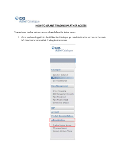
Why are Derivative Warrants More Expensive than
Options? An Empirical Study
Gang Li and Chu Zhang∗
This version: May, 2009
∗ Li,
[email protected], Hong Kong Baptist University (HKBU), Kowloon Tong, Kowloon,
Hong Kong and Zhang, [email protected], Hong Kong University of Science and Technology
(HKUST), Clear Water Bay, Kowloon, Hong Kong. We would like to thank Du Du, George
Jiang, Nengjiu Ju, Ming Liu, Sophie Ni, Qian Sun, Yexiao Xu, seminar participants at 2008
China International Conference in Finance and Universities of Fudan, HKBU, HKUST, Macau,
and Xiamen, and especially the anonymous referee for helpful comments on earlier versions of the
paper. Chu Zhang acknowledges financial support from HKUST research project competition
grant, RPC06/07.BM28. All remaining errors are ours.
Why are Derivative Warrants More Expensive than
Options? An Empirical Study
Abstract
Derivative warrants typically have higher prices than do otherwise identical options.
Using data from the Hong Kong market during 2002-2007, we show that the price difference reflects the liquidity premium of derivative warrants over options. Newly issued
derivative warrants are much more liquid than are options with similar terms. As a result, long-term derivative warrants are preferred by traders who trade frequently. In spite
of their higher prices, short-term returns on long-term derivative warrants are, in fact,
higher than the hypothetical short-term returns on options. The differences in price and
liquidity measures decline as the contracts get closer to maturity.
I.
Introduction
The call and put derivative warrants traded in many markets are like usual call and
put options traded in the US and elsewhere, except that they can be issued (i.e., sold
short) only by certain financial institutions approved by regulators. It has been observed
that derivative warrants tend to be priced higher than otherwise identical options. This
phenomenon, which is in violation of the law of one price, a central theme in financial
economics, is the focus of the current paper. Our objective is to understand what causes
derivative warrants and options with identical payoffs to have different prices and how
they can coexist in the market.
The main thrust of our investigation is the difference in liquidity between derivative
warrants and options. The effect of liquidity on asset pricing has received considerable
attention in the literature in recent years. In their seminal work, Amihud and Mendelson
(1986) provide a theoretical argument that illiquidity caused by higher bid-ask spreads
leads to price discounts and higher expected returns. There are many empirical studies
on primitive assets confirming this theory.1 On the liquidity effects on derivative assets,
recent works include Jarrow and Potter (2008), Cetin, Jarrow, Protter, and Warachka
(2006), Garleanu, Pedersen, and Poteshman (2007) and Deuskar, Gupta, and Subrahmanyam (2008). What makes derivatives, and especially options, special is that derivatives are in zero net supply. As buyers require price discounts on illiquid derivatives,
sellers require price premiums. Whether illiquid derivatives carry a price discount or a
price premium, as Deuskar at el. (2008) argue, depends on whether the marginal trader is
a buyer or a seller, on the risk appetite of the marginal trader, on the extent to which the
Amihud and Mendelson (1989) and Brennan and Subrahmanyam (1996) find that illiquid stocks are
traded at lower prices and have higher expected returns when other factors are controlled. Amihud and
Mendelson (1991) find that the less liquid Treasury notes have lower prices and higher yields-to-maturity.
Silber (1991) find that restricted stocks which are prohibited to trade in the open market are sold at
an average discount of 33.75%. Chan, Hong, and Subrahmanyam (2006) find that a higher premium
on American Depositary Receipts (ADR) is associated with higher ADR liquidity and lower home share
liquidity.
1
1
derivative cannot be replicated by primitive assets, and on the nature of the illiquidity.
As liquidity is a broad concept with many dimensions, it is possible that some notions of
illiquidity cause price discounts on derivative assets while other notions of illiquidity lead
to price premiums. Brenner, Eldor, and Hauser (2001) find that non-tradable options are
priced at a mean discount of 18% to 21% of the exchange-traded synthetic options with
the same payoff and conclude that this form of illiquidity has an negative effect on derivative prices. On the other hand, some derivatives are demanded by investors for hedging
and speculation, but there are few sellers around. Because of stochastic volatility, jumps,
discrete rebalancing, transaction costs, and illiquidity of the underlying assets, derivatives cannot be replicated without costs. The buying pressure combined with illiquidity
in this situation leads to price premiums. Deusker et al. (2008) document substantial
price premiums on over-the-counter interest rate caps and floors as dealers need to cover
costs in hedging their short positions. A similar phenomenon documented by Bollen and
Whaley (2004) is the overpricing of out-of-the-money S&P 500 index put options which
are bought by investors for hedging potential losses in large stocks, with few sellers.
We investigate the difference in prices of derivative warrants and options written on the
Hang Seng Index (HSI) in the Hong Kong market. The Hong Kong derivative warrants
market is the largest in the world in terms of trading volume.2 There is an advantage
of our study of the liquidity effects on derivative prices over the existing studies. Unlike
most other studies that involve inferring the price of the otherwise identical liquid asset
for a given illiquid asset, both derivative warrants and options are traded in the market
and their prices are directly observed. In addition, a variety of liquidity measures for both
types of derivatives can be easily constructed. We use a matched sample of derivative
warrants and options so that other factors affecting derivative prices, but unrelated to
liquidity, are controlled. The quantitative relationship between the price difference and
Derivative warrants are traded in Germany, Switzerland, Italy, Britain, Australia, Hong Kong, Singapore, Korea and some other countries under different names. Derivative warrant is the term used in
Hong Kong.
2
2
liquidity differences can be more easily examined. Our empirical results show that by
the standard measures of liquidity, including bid-ask spread, trading volume, turnover
ratio, contract size and the Amihud (2002) measure, long-term derivative warrants are
much more liquid than are options. These results suggest that the overpricing of derivative
warrants is explained by the liquidity differences between derivative warrants and options.
The fact that derivative warrants are traded at higher prices than are options indicates
that the illiquidity in these dimensions entails price discounts, consistent with Brenner et
al.’s (2001) findings. The results presented in this paper are also consistent with Deuskar
et al.’s (2008) argument regarding liquidity and price premiums/discounts. Since this is
not the focus of the paper, we defer further discussions to the last section.
The results on turnover ratios imply that about a half of the derivative warrants have
a holding period of less than two weeks, and about 20% have a holding period of less
than one day. On the contrary, about 80% of options contracts have a holding period of
longer than one month. Derivative warrants are more frequently traded than are options.
We further investigate the returns on derivative warrants and options for different holding
periods, using ask prices for initial buying and bid prices for later selling. It turns out that
short-term holding period returns on derivative warrants are mostly higher than those on
the corresponding options, although derivative warrants are bought at higher prices. As
the holding period gets longer, the return difference between derivative warrants and the
corresponding options becomes narrower. Eventually, the returns on options are higher
than those of derivative warrants. These results are a manifestation of the clientele effect,
proposed by Amihud and Mendelson (1986), that investors with different holding periods
maximize the after-transaction-cost expected returns, which leads to a phenomenon, in
equilibrium, that the assets with larger bid-ask spreads are held by investors with longer
holding periods.
Our work is also related to Chan and Pinder (2000) who study the derivative warrants
market in Australia and find overpricing of derivative warrants relative to options. They
3
show that the trading volume of derivative warrants relative to that of options can explain
some of the overpricing among other variables such as days-to-maturity, the presence of
market makers in the options market, and the identity of warrants issuers. We account
for the overpricing of derivative warrants with a full range of liquidity measures. We
also go one step further to analyze the holding period returns on derivative warrants and
options. Our results indicate more clearly that two assets with identical cash flows but
with different prices can coexist in the market if the transaction costs are different and
that the more liquid derivative warrants market caters to the short-term trading needs
of investors. There are other studies of derivative warrants, especially on the Hong Kong
market, but they are unrelated to warrant overpricing.3
The remainder of this paper is organized as follows. Section 2 describes the Hong
Kong derivative warrants and options markets. Section 3 describes the data. Section 4
provides evidence of overpricing of derivative warrants relative to options and presents
the main results on overpricing and liquidity. Section 5 compares holding period returns
on derivative warrants and options. Section 6 concludes the paper.
II.
The Derivative Warrants and Options Markets in
Hong Kong
Trading of derivative warrants and options in Hong Kong is conducted in the Hong Kong
Exchange and Clearing Limited (HKEx), which is divided into the Securities Market and
the Derivatives Market. The Securities Market is also known as the Stock Exchange. For
historic reasons, stocks and derivative warrants are traded on the Stock Exchange. The
Derivatives Market is further divided into the Futures Exchange and the Stock Options
Duan and Yan (1999) use a semi-parametric approach to pricing derivative warrants that substantially
improves upon the Black-Scholes model. Several papers in the literature focus on the effect of the
introduction of derivative warrants on the price and trading volume of the underlying securities, for
example, Chan and Wei (2001), Chen and Wu (2001) and Draper, Mak, and Tang (2001). A recent paper
by Chow, Li, and Liu (2007) examines the trading records of market makers in the Hong Kong derivative
warrants market to understand their inventory management.
3
4
Exchange. Index futures and index options, among others, are traded on the Futures
Exchange, while options on individual stocks are traded on the Stock Options Exchange.
There are two types of warrants listed on the Hong Kong Stock Exchange: equity
warrants and derivative warrants. Equity warrants, issued by the underlying company
itself, entitle holders to purchase equity securities from the underlying company at a predetermined price. Derivative call warrants are similar to equity warrants except that they
are issued by a third party, usually a financial institution. Derivative put warrants, also
issued by a third party, entitle holders to sell equity securities of an underlying company
at a pre-determined price to the issuer. In Hong Kong, trading of equity warrants started
in 1977, while trading of derivative warrants started in 1989. In recent years, the bulk
of the warrants traded on the Hong Kong Stock Exchange are derivative warrants. The
underlying assets of the derivative warrants are mostly blue-chip stocks. Other underlying
assets include stock indexes, baskets of stocks, and some commodities. All the derivative
warrants are of European style. The issuers of derivative warrants are typically largeand medium-sized financial institutions. Several major European and Australian banks,
such as Societe Generale, KBC, Deutsche Bank, BNP Paribas, and Macquarie Bank, are
among the most active issuers. Each underlying asset may have multiple issuers who
compete with each other to offer popular contract specifications, lower prices and better
liquidity.
Options trading in Hong Kong started in March 1993. Initially, only options written
on the HSI were introduced. Trading of options on individual stocks started in September
1995. The index options are of European style and settled by cash, while the stock options
are of American style with physical delivery of the underlying assets upon exercise. The
contract specifications of the options are set by the exchange. A system of market makers
has been implemented whereby a handful of market makers is involved. At the end of
2007, there were 18 market makers in the Futures Exchange and about 30 market makers
in the Stock Options Exchange. The market makers are required to provide liquidity to
5
the trading system. The requirements are not stringent, however. For options expiring
in the nearest three months with near-the-money strikes, market makers are required to
provide continuous quotes, while for all others, they only need to respond to requests for
quotes.
Panels A and B of Figure 1 plot the total trading volume of derivative warrants and
options in terms of billions of Hong Kong dollars (HKD) over the period 2002-2007. The
derivative warrants have gained much popularity over time with their trading volume
increasing from about 7 billion HKD per month in 2002 to 397 billion HKD per month
in 2007. By the end of 2006, the Hong Kong derivative warrants market had become
the largest derivative warrants market in the world in terms of trading volume and it
accounted for one-third of the total trading volume on the Hong Kong Stock Exchange.
The trading volume of options in Hong Kong grew at a moderate pace from about 1.04
billion HKD per month in 2002 to 14.2 billion HKD per month in 2007, which pales in
comparison to the trading volume of derivative warrants.
Figure 1 here
The rapid growth of the derivative warrants market in Hong Kong owes much to
certain regulatory changes made in late 2001. Before these changes, issuers were required
to place at least 85% of a derivative warrants issue with more than 100 investors on the
issue date (or more than 50 investors if the size of the warrant issue was small). This
exerted substantial pressure on the issuers. The 2001 rule repealed that requirement so
that issuers could sell an entire issue gradually over time. The 2001 rule also required
that each issuer appoint a liquidity provider to input bid and ask prices in the trading
system, either continuously or on request. The new rules improved the liquidity of the
derivative warrants market substantially.
Another factor that contributes to the relative liquidity of derivative warrants over
options is their minimum trading size. Set by the exchange, a round lot of options
6
on stocks is the same as that of underlying stocks. However, a round lot of derivative
warrants, determined by the issuer, is typically only one-tenth of that of underlying stocks.
This facilitates speculative trading by many small investors.
There is much anecdotal evidence that options and derivative warrants have different
clienteles. In a survey conducted by the HKEx, 50.7% of respondents revealed that they
used the HSI options for pure trading, 37.4% for hedging, and 12% for arbitrage. Among
the investors, only 24% were local and overseas retail investors and the remaining were
either market makers, proprietary traders, or local and overseas institutional investors.
In the derivative warrants market, most traders are individual investors and they tend to
hold warrants for only short periods. A survey conducted in 2006 by the Hong Kong Securities and Futures Commission revealed that 86.8% of the respondents traded derivative
warrants for short-term gains and only 0.4% of the respondents used derivative warrants
for long-term investments.
It should be noted that issuers of derivative warrants in Hong Kong are not required
to hold the underlying assets, thus it is possible that derivative warrants may not be
covered. On the other hand, options in Hong Kong are settled by the Hong Kong Futures
Exchange Clearing Corporation and a margin is required for short positions. As a result,
derivative warrants have higher credit risk than do options, therefore, other things being
equal, derivative warrants should be traded at lower prices than options are traded. We
show in Section 4.A, however, that derivative warrants tend to have higher prices than
do options.
III.
A.
Data Description
Price Data
We focus on derivative warrants and options written on the HSI in this paper. A comparison between derivative warrants and options on the index is clean as they are both
7
of European style and cash-settled. The HSI is the benchmark index in the Hong Kong
stock market and the derivatives written on it are the most liquid ones. For the rest of
the paper, we will refer to derivative warrants on the HSI as just warrants because the
underlying is an index and there is no confusion.
The data on warrants and options on the HSI are obtained from the HKEx. The warrants data include daily closing bid and ask prices, trading share volume, dollar volume,
and other contract specifications such as maturity and strike price. The HKEx requires
liquidity providers to disseminate the number of shares bought or sold, the average buying and selling prices, and the amount of warrants outstanding on a daily basis. Such
information is available from the HKEx website. The options data include daily closing
bid and ask prices, trading volume, open interest, maturity and strike price of the options.
The HSI level is from Datastream. We use two samples of warrants and options matched
with the same maturity and strike price. One sample, named TQ, consists of daily closing quotes with positive trading volume for warrants. In about one-third of this sample,
the daily trading volume of options is zero. The other sample, named TT, consists of
daily closing quotes with positive trading volumes for both warrants and options. Unless
otherwise stated, all the results below are based on the TT sample. The sample period
is from July 15, 2002 to December 31, 2007. Before this starting date, data on options
are not available. There are many missing closing bid and ask quotes for the option data
provided by the HKEx. We use the intraday option bid and ask quotes as supplements.4
Panels C and D of Figure 1 plot the trading volume of warrants and options on the
HSI during the sample period. The total trading volume of the warrants on the HSI
increased from about 2.65 billion HKD per month in 2002 to about 81 billion HKD per
month in 2007. However, the trading volume of the options on the HSI experienced only
a moderate increase from about 0.75 billion HKD per month in 2002 to about 10 billion
HKD per month in 2007. As we saw earlier for the whole market, the growth of the
We select the quote that is the closest to 4:00 pm, no earlier than 3:45 pm, and no later than 4:15
pm, because the warrants market is closed at 4:00 pm.
4
8
warrants on the HSI has been much faster than that of the options on the HSI.
We denote the value of the HSI on business day t as H(t) and the strike price of
a warrant or an option as K. Let pbw (t, κ, m) and paw (t, κ, m) be the closing bid and
ask prices, respectively, of a warrant (either a call or a put) on day t with moneyness,
κ = 1 − K/H(t) for a call and κ = K/H(t) − 1 for a put, and maturity, m, measured by
the number of days. Similarly, let pbo (t, κ, m) and pao (t, κ, m) be the bid and ask closing
prices, respectively, of the option (either a call or a put) on day t with moneyness, κ,
and maturity, m. Warrants with the same (κ, m) issued by different issuers are treated as
separate observations, but matched with the same option. For simplicity, the dependence
of κ on t is suppressed unless it is necessary.
We divide the entire matched sample into several groups according to moneyness and
maturity. Moneyness is divided into the groups of κ ≤ −0.03 (out-of-the-money, OTM),
−0.03 < κ ≤ 0.03 (at-the-money, ATM) and κ > 0.03 (in-the-money, ITM). Maturity is
divided into the groups of short term (ST) with m ≤ 60 days, medium term (MT) with
60 < m ≤ 120 days and long term (LT) with m > 120 days. If there are less than eight
pairs of matched warrants and options within a group in a week, we regard the week as a
missing week for that group. Table 1 shows the weekly average number of matched pairs
of warrants and options and the non-missing weeks in each of moneyness and maturity
groups. There are about 235 matched pairs of warrants and options each week on average
and the majority of the groups have more than 160 non-missing weeks in the sample.
The average of bid-ask average price of warrants, P¯w = 100(paw + pbw )/2H, and of options,
P¯o = 100(pao + pbo )/2H, of various moneyness-maturity groups are reported in Table 1.
The reason for normalizing by H is to make the price data comparable across time, as
the values of the HSI and the values of derivatives written on it contain an upward trend.
Defined this way, the prices of warrants or options are expressed in terms of the percentage
of the HSI level. In all the groups, the prices of warrants are higher than those of options,
and the overpricing is the highest for the LT groups.
9
Table 1 here
B.
Liquidity Variables
We employ a number of variables to measure the liquidity of warrants and options contracts. We focus on liquidity, rather than liquidity risk, in this paper. The former refers
to the tradability of a security without adverse market impact, while the latter refers to
the unpredictable changes in liquidity over time as well as their relationship with marketwide liquidity factors. The liquidity measures we examine include the bid-ask spread,
the trading volume, the Amihud illiquidity measure, the turnover ratio, the contract size
and the percentage of trading by liquidity providers. Among the liquidity measures, the
bid-ask spread is based on quotes, while the other measures are based on transactions.
Each variable measures one aspect of liquidity.
The bid-ask spread is widely used in the literature. Table 1 reports the average bidask spread for warrants, Sw = 100(paw − pbw )/H, and for options, So = 100(pao − pbo )/H,
in each moneyness-maturity group. Similar to the price measure, the bid-ask spread is
expressed in the percentage of the HSI level. The bid-ask spreads of warrants are generally
decreasing with maturity. However, they generally increase with maturity for options.
The second measure we consider is trading volume. We report in Table 1 the group
average of Vw /1000H and Vo /1000H, where Vw and Vo are the daily dollar trading volumes
for warrant and option contracts, respectively. Similarly, we normalize the dollar volume
by the HSI level to adjust for the upward trend. Warrants are much more actively traded
than are options in most of the groups. The trading volume is distributed differently
across maturity groups for the warrants and the options. Most of trading volume of the
warrants is concentrated in the MT and LT groups. Options, however, have the largest
volume in the ATM-ST group.
A popular measure of illiquidity is the Amihud (2002) measure, which has been used
10
in numerous studies. The measure is based on Kyle’s (1985) λ, the response of prices to
order flow. The Amihud illiquidity measure, A(t, κt , m), is defined as
(1)
5
1 X |R(t + i, κt+i , m − i)|
,
A(t, κt , m) =
11 i=−5 V (t + i, κt+i , m − i)/1000
where |R(t, κt , m)| is the daily absolute percentage return on a contract with (κt , m) on day
t. The Amihud measure is defined only for observations with positive trading volumes. We
winsorize the measure at 2 for both the warrants and options, which roughly corresponds
to the 99th percentile of the distribution. Table 1 shows that the Amihud measure is in
general lower for the warrants than for the options for the MT and LT groups, but higher
for the ST groups. Across moneyness, the OTM warrants and options have a higher
Amihud measure than the ITM counterparts have.
The trading in the warrants market is more active than that in the options market as
evidenced by the difference in the daily dollar trading volumes between the two markets.
Alternatively, we can measure the trading activity in each market by the turnover ratio,
the frequency of a share changing hands, within a given period. The reciprocal of the
turnover ratio is usually interpreted as the average holding period by investors. For
warrants and options, however, some modifications are needed because the outstanding
amount changes over time, unlike the case of stocks and bonds. The turnover ratio of a
warrant contract, Tw (t, κ, m), is defined as
(2)
[Uw (t, κt , m) − Nw (t, κt , m)] − 21 [UwL (t, κt , m) − Nw (t, κt , m)]
Tw (t, κ, m) =
,
Ow (t − 1, κt−1 , m + 1)
where Uw (t, κt , m) is the trading volume of the warrant with (κt , m) on day t expressed
by the number of shares, UwL (t, κt , m) is the number of the warrants with (κt , m) on day
t traded by the liquidity provider, Ow (t, κt , m) is the outstanding amount of the warrant
with (κt , m) on day t, and Nw (t, κt , m) = max[Ow (t, κt , m) − Ow (t − 1, κt−1 , m + 1), 0] is
the new issues of the warrants. The new issues are subtracted because the turnover ratio
is defined for existing contracts. Half of the trading by liquidity providers is subtracted
11
to avoid double counting.5 This definition assumes that liquidity traders always trade
to provide liquidity to customers and never trade for themselves. Liquidity providers do
trade for themselves sometimes, but we do not have the data to distinguish between the
trades by liquidity providers for themselves and those for customers. The above definition
may, therefore, underestimate the actual turnover ratio.
The turnover ratio for an option contract, To (t, κ, m), is defined as
(3)
To (t, κ, m) =
Uo (t, κt , m) − No (t, κt , m)
,
Oo (t − 1, κt−1 , m + 1)
where Uo (t, κt , m) is the trading volume in contracts of the option with (κt , m) on day t,
Oo (t, κt , m) is the outstanding amount of the option with (κt , m) on day t, and No (t, κt , m) =
max[Oo (t, κt , m) − Oo (t − 1, κt−1 , m + 1), 0] is the number of new contracts with the same
terms. Like the definition of turnover ratio for warrants, No (t, κt , m) is subtracted to
exclude the new option contracts in calculating the turnover ratio. However, we do not
have the information on the amount of trading by option market makers. We assume that
all the trades are between customers and, therefore, the turnover ratio of options defined
this way may overestimate the actual turnover ratio.
Table 1 reports the group average of Tw and To . The turnover ratio of the warrants
tends to decrease as the maturity decreases, while the turnover ratio of the options tends
to increase as the maturity decreases. In the MT and LT groups, the turnover ratio of the
warrants is many times higher than that of the options. The turnover ratio in the ATM
groups of warrants tends to be higher than that of the ITM and OTM groups. For the
options, the ATM and OTM groups have a higher turnover ratio than the ITM groups.6
These turnover ratios imply roughly that the average holding period of the warrants
is between one day to one week and that the average holding period of the options is
A direct trade between two customers is counted just once. A trade between two customers through
a liquidity provider is counted twice in Uw and UwL .
6
Turnover ratios are highly positively skewed. For the warrants, the median of turnover ratios for the
ATM are 0.23, 0.42 and 1.65 for the ST, MT and LT group, respectively, and they are higher than the
ITM and OTM groups. For the options sample, the ATM-ST group has the highest median turnover
ratio of 0.04.
5
12
about one month. Recall that the turnover ratio of the warrants may be underestimated,
while the turnover ratio of the options may be overestimated. The actual situation may
therefore be more extreme than what we describe here.
The next measure we consider is the contract size, which is the number of underlying
assets for one round lot of warrants, or one contract of options. The contract size matters because there is a large number of small, individual investors in terms of personal
wealth who trade derivative warrants for increasing leverage. They can participate in the
market only when they can afford to buy the minimum amount. A small contract size
facilitates these trades. Let Cw and Co denote the contract size for warrants and options,
respectively. Table 1 shows that the average contract size for the warrants is about 2.4
HSI, while one contract of options always corresponds to 50 HSI. The minimum dollar
amount for buying warrants is typically below five thousand HKD, which makes the warrants market accessible to small, individual investors. The options contracts, however,
typically cost tens of thousands of HKD. In fact, 45.4 percent of warrants transactions
have actual trading sizes below 50 HSI, and 24.8 percent are below 25 HSI. The trading
volume of warrants with actual trading sizes below 25 HSI exceeds the entire trading
volume of options on HSI in the TT sample. In this sense, the warrants market plays an
indispensable role for small individual investors.
The percentage of warrant trading by liquidity providers is calculated as the share
volume traded by liquidity providers divided by the total share volume for a warrant
contract on a day on which the total trading volume is positive, Lw = UwL /Uw . The
higher the value, the more actively liquidity providers supply liquidity to the market by
quoting the best bid and ask prices. In general, liquidity providers supply liquidity quite
actively. The average Lw for the entire sample is 67.67%. Table 1 shows that, for the LT
warrants, about 90% of trading involves liquidity providers. Across moneyness, liquidity
providers trade the ITM warrants more actively than they trade the OTM warrants.
There is no data on what percentage market makers of options trade. Therefore, Lo is
13
unavailable.
Panel A of Table 2 reports the correlations among price, P¯ , maturity, m, moneyness, κ,
and the liquidity measures. Since V and T are positively skewed, we define V˜ = log(V /H+
1) and T˜ = log(T +1), which are also used in the regression analysis in the next section. We
put a negative sign in front of S, C and A to define all the measures as liquidity measures.
The upper triangle is for the TQ sample with a positive trading volume of warrants, but
possibly no trading of options. A for the TQ sample is undefined. The lower triangle
is for the TT sample with positive trading volumes of both warrants and options. The
correlations reported are the time-series averages of the weekly cross-sectional correlations.
The results show that the price is positively correlated with maturity and, especially, with
moneyness. The liquidity measures are positively related to m and κ, except for −S. All
the liquidity measures are moderately, positively related. The highest pair is −C and L.
This is because all warrants have low values of C and high values of L, and options are the
opposite. Comparatively, the correlations of −A with other liquidity measures are lower.
The magnitudes of the correlations across the two samples are comparable. Panel B of
Table 2 reports the correlations among the price difference, DP¯ , maturity, m, moneyness,
κ, and the liquidity differences between the matched warrants and options pairs. The
price difference is highly correlated with maturity, but not so with moneyness. The
correlations between liquidity differences are mostly lower than the correlation between
liquidity measures in Panel A.
Table 2 here
IV.
A.
Overpricing and Liquidity
Overpricing
In this subsection, we document the overpricing of warrants relative to options. Let
Pwa = 100paw /H, Pwb = 100pbw /H, Poa = 100pao /H, and Pob = 100pbo /H. Panel A of Table
14
3 reports the proportion of the observations for which the warrant price is greater than
the matched option price, where the price is set as the bid, ask, or bid-ask average. Most
warrants are traded at higher prices than are their options counterparts. The proportions
for P¯w > P¯o are above 80%, except for the ITM-ST group. The proportion is higher
for the LT groups than for the ST groups and higher for the OTM groups than for
the ITM groups. The patterns in the proportions of Pwa > Poa and of Pwb > Pob are
similar. The case of Pwb > Poa is an arbitrage opportunity for those who can sell the
warrant, buy the matched option, and keep the position to maturity. The proportions of
Pwb > Poa for the LT groups are almost as high as those for P¯w > P¯o . While individual
investors cannot sell warrants short, why don’t they sell what they already own and
buy the matched options? In addition, why don’t warrant issuers sell more overpriced
warrants and hedge their positions with the matched options? These are the questions
that make the overpricing phenomenon nontrivial. We will return to these questions in
the following sections. For completeness, the proportions of Pwa > Pob are also reported.
These proportions are virtually 100%, meaning that profitable opportunities for buying
warrants, selling the matched options, and holding them to maturity are rare, although
these actions are feasible for individual investors. Such contracts are mainly concentrated
in the ITM-ST group.
Table 3 here
Panel B of Table 3 reports the time-series averages of the cross-sectional average price
differences for each moneyness-maturity group, with their t-ratios. The average price
differences, P¯w − P¯o , Pwa − Poa , and Pwb − Pob , are all significantly greater than zero, except
for the ITM-ST group for Pwb − Pob . Overall, call warrants are more overpriced than put
warrants. When the transaction costs are taken into account, the averages of Pwb − Poa are
much smaller in magnitude and the significance is also reduced. In particular, overpricing
tends to become insignificant, or even reversed, in the ST groups. For completeness and
comparisons, the averages of Pwa − Pob are also included.
15
B.
Liquidity Differences
In this subsection, we present the evidence that the liquidity measures are also different
between the warrants and the matched options. In Panel A of Table 4, we report the
proportion of which the liquidity (illiquidity) measure of a warrant is greater (less) than
that of the matched option. For the LT and MT groups, the proportion is higher than 50%
for all the liquidity measures. Only for the OTM-ST group is the proportion substantially
less than 50% for Sw < So , Vw > Vo and Tw > To . The results also show that all warrants
have smaller minimum contract sizes than do options.
Table 4 here
Panel B of Table 4 reports the time-series average of the cross-sectional average liquidity measure differences for each moneyness-maturity group, with their t-ratios. Negative
signs are put in front of the illiquidity measures. For (Vw − Vo )/1000H, Tw − To and
−(Cw − Co ), the differences in the liquidity measures are positive for all the moneynessmaturity groups, and the majority of them are significant. For the other two liquidity
measures, −(Sw − So ) and −(Aw − Ao ), the differences for the MT and LT groups are
mostly positive and significant, but some of the differences for the ST groups are negative.
C.
Analysis-of-Variance
In standard options pricing theory, warrants/options prices normalized by the price of
the underlying asset depend on their moneyness, maturity, the stochastic volatility of the
underlying asset, and the other state variables that govern the evolution of the price of
the underlying asset. The central theme of this paper is that warrants/options prices also
depend on their liquidity. To establish the dependence of the warrants/options prices on
liquidity, we need to separate the effects of other variables. As we see in Table 2, both
prices and liquidity measures are correlated with the maturity. It is important to remove
16
the maturity effect to avoid finding potential spurious relationships. To deal with this, we
pool the matched warrants and options pairs together and run the following regression,
(4)
P¯ = b1 + b2 κ + b3 m + b4 σ + P˜ ,
where P¯ is P¯w or P¯o and σ is the stochastic volatility of the HSI estimated with daily
returns on the HSI from 1998 to 2007 using the so-called GJR-GARCH model of Glosten,
Jagannathan, and Runkle (1993). The regression is run for each moneyness-maturity
group using pooled cross-section and time-series data. While the true relationship of warrants/options prices with moneyness, maturity, and stochastic volatility may be nonlinear,
estimating a linear relationship within a moneyness-maturity group reduces the error of
linear approximation.7 The residual, P˜ , mainly captures omitted liquidity effects, the
approximation error from the linear term of the stochastic volatility, and other omitted
state variables. We investigate the relationship between P˜ and liquidity measures in the
following subsections. In this subsection, we further characterize the overpricing of warrants relative to options by conducting an analysis-of-variance for the normalized price
unexplained by moneyness, maturity and stochastic volatility.
Panel A of Table 5 reports the mean of P˜ for the warrants and the options separately.
The means of price residuals for warrants are all positive, while the means of price residuals
for options are all negative. The differences in means between the warrants and options
reflect the between-type variation in the price residuals, P˜ . Panel A also shows that the
overpricing of warrants is the largest for the LT groups. Panel B of Table 5 reports the
standard deviation of P˜ for the warrants and the options separately and combined. The
total variation of the combined sample is larger than that of separate warrants sample
or separate options sample for most of the groups. The standard deviations of P˜w and
of P˜o indicate the within-type variation of P˜ . For some LT groups, the variation of the
combined sample is about two times as large as that of the separate samples. The last
As a robustness check, we also regress P¯ on κ, m and σ nonparametrically across all the moneynessmaturity groups to obtain the price residuals P˜ . The results are quantitatively similar.
7
17
part of Panel B in Table 5 reports the standard deviation of the price residual difference
P˜w − P˜o , which is the same as the price difference, P¯w − P¯o , because warrants and options
are matched pairs. The variation in the price residual difference is considerably smaller
than that in the combined price residual sample, but it is non-trivial. In the next two
subsections, we ask why warrants are more expensive than options and why some warrants
are more overpriced than other warrants.
Table 5 here
D.
Why are Warrants More Expensive than Options?
In this subsection, we use regression analysis to quantify the overpricing of warrants
relative to the options as contributed by the liquidity difference between the warrants and
the options. We run regressions of the price residuals obtained in the last subsection on
various measures of liquidity,
(5)
P˜ = β1 + β2 (−S) + β3 (−C) + β4 V˜ + β5 T˜ + β6 L + β7 (−A) + ε.
We run the regressions with each liquidity measure separately, with all the liquidity measures together except for L, and with all the liquidity measures together where L for an
option is arguably set to zero. We run the regressions for the TQ sample, in which A
is undefined when there is no trading volume for options, and for the TT sample. The
cross-sectional regressions are run for each moneyness-maturity group in each week. The
slope coefficients are averaged across groups first and then averaged across weeks. The
results are reported in Table 6. For each regression, the first row shows the coefficient
estimates. The second row shows the coefficient estimates multiplied by the standard
deviation of the corresponding independent variable, so that the number measures the
change in the dependant variable for one standard deviation change in the independent
variables. The third row reports the t-statistics of the coefficient adjusted for 10-week
lags in the autocorrelations using the Newey and West (1987) procedure. In Panel A
18
for the TQ sample, all the liquidity variables are significant in the univariate regressions
with the expected signs. The unit variation in T˜ and S explains most of the variation in
P˜ . In the multiple regressions, the transformed trading volume, V˜ , loses its explanatory
power. The coefficients of −S, −C and T˜ are all significant without the presence of L
and their explanatory power reduces with the presence of L. In Panel B for the TT sample, the slope coefficients of all the liquidity variables, including the Amihud measure, A,
have expected signs and are significant in the univariate regressions. Again, V˜ loses its
explanatory power in multiple regressions, as does A.
Table 6 here
E.
Why are Some Warrants More Overpriced than Other Warrants?
Short-term warrants tend to be less overpriced relative to options, or they are even underpriced. Within a moneyness-maturity group, there are non-trivial variations in the
price differences between the matched warrants and options, DP = P¯w − P¯o , as we see in
Table 5. In this subsection we investigate if the variations in DP can be explained by the
variations in the difference of liquidity variables between matched warrants and options.
We run regressions of the price difference on liquidity differences,
(6)
DP = β1 + β2 (−DS ) + β3 (−DC ) + β4 DV + β5 DT + β6 Lw + β7 (−DA ) + ε,
where DS , DC , DV , DT , and DA are the differences between warrants and options in S, C,
V˜ , T˜ and A, respectively. The regressions are run for each moneyness-maturity group for
each week and the slope coefficients are then aggregated across groups and across weeks
like those in Table 6.8 Table 7 reports the results.
The price difference across the moneyness-maturity groups appears to be related to H, σ, and m.
As an alternative approach, we remove the effects of those variables by regressing DP /Hσm on liquidity
variables for observations pooled across moneyness-maturity groups. We also consider a more sophisti+
−
cated way of adjusting the price difference, DP /Hσ(m + a)α0 +α1 κ +α2 κ , where κ+ = max(κ, 0) and
κ− = max(−κ, 0), and the parameters are estimated from warrants and options data. All the results are
essentially the same.
8
19
Table 7 here
For the TQ sample in Panel A, each liquidity measure has the expected sign in the
univariate regressions. The slope coefficient of −DC , however, is not very significant.
Since the minimum contract size of the options is a constant (i.e., 50 shares of HSI),
the variation in −DC is just the variation in Cw . This highlights the differences in the
regressions of prices in Table 6 and the regressions of price differences in Table 7. In
price regressions, −C is useful in explaining the variation in prices as the contract size of
options is too large for small individual investors to trade. But among all the warrants
whose minimum trading sizes are all small enough, the variation in their minimum trading
size is not the major concern for the investors to choose one warrant over another. In the
multiple regression, DC gains some explanatory power, DV , however, loses its explanatory
power as in the price regression in Table 6. For the TT sample in Panel B, the coefficients
of DC and DA are insignificant in the univariate regressions. In the multiple regressions,
the coefficient of DA is also insignificant and the coefficient of DV has the wrong sign,
while other liquidity differences remain useful in explaining the price difference.
V.
Overpricing and Holding Period Returns
Since the payoff for the matched warrants and options on the maturity dates are the same,
if a warrant has a higher price than the corresponding option and they are both held to
maturity, the return on the warrant must be dominated by the return on the option. From
our earlier analysis, we see that long-maturity warrants tend to have very high turnover
ratios, which implies that long-maturity warrants have very short holding periods. Are
returns on warrants necessarily dominated by those on options for short holding periods?
The answer is not obvious for two reasons. The first reason is transaction costs. The
bid-ask spread tends to be smaller for warrants than for options, especially long-maturity
ones. The second reason is that overpricing is not always monotonic with maturity. If a
20
warrant is bought at a price higher than the otherwise identical option, but it is also sold
later at an even higher price than the option, the holding period return on the warrant
can be higher than that on the corresponding option.
We examine the difference in holding-period returns between the warrants and the
options from a buyer’s point of view only because the warrants can not be sold short by
anyone other than approved issuers. The holding-period return in percentage is defined
over the ask price on day t − i and the bid price on day t, standardized to the daily basis
as
(7)
(8)
i
Rw
(t, κt , m) = 100
Roi (t, κt , m) = 100
"
"
Pwb (t, κt , m)
Pwa (t − i, κt−i , m + i)
1/i
Pob (t, κt , m)
Poa (t − i, κt−i , m + i)
1/i
#
−1 ,
#
−1 ,
where i = 1, 7, 14, 28 for one-day, one-week, two-week and four-week returns. Table 8
reports the average differences in the holding period returns between warrants and options
for each moneyness-maturity group using all matched contracts for the TT sample.9
Table 8 here
The results indicate that for short holding periods such as one day, the consideration
of transaction costs outweighs that of pricing in determining returns. Taking bid-ask
spreads into account, the one-day average holding period returns of warrants sample are
significantly higher than those of options in the majority of the groups. As the holding
period becomes longer, the convergence of the warrants payoff and the options payoff takes
effect and the initial pricing becomes important. For the one-week holding period, the
average return differences in some of the ST groups are significantly negative. However,
the average return differences are still positive in many of the MT and LT groups. For
the case of four-week holding periods, the average return differences are negative in the
9
The TQ sample gives quantitatively similar results.
21
majority of the groups and many of them are significant. The contrast between one-day
and four-week return differences suggests that investors who have short-term trading in
mind should trade warrants because the transaction costs are lower, while investors with
long holding periods should trade options as returns on options tend to be higher due to
lower initial prices.
VI.
Conclusion
In this paper, we study the overpricing of derivative warrants relative to options in Hong
Kong. We find that the majority of derivative warrants written on the Hang Seng Index
are traded at higher prices than are options with the same underlying asset, strike price
and maturity. Derivative warrants are also much more liquid than are the options. We
use a number of standard liquidity measures in the literature, namely, bid-ask spread,
trading volume, contract size, turnover ratio, and the Amihud illiquidity measure to
explain the overpricing phenomenon. The regression analysis shows that these liquidity
measures explain the overpricing of derivative warrants to a large extent. We also use a
unique liquidity measure for the derivative warrants, the percentage of trading volume by
liquidity providers that measures how actively the liquidity providers supply liquidity for
their derivative warrant contracts. This additional variable contributes a large portion
of explanatory power in the regression analysis. The regression results also indicate that
while all the liquidity measures explain why the warrant prices tend to be higher than
option prices, many of them are also useful in explaining why some derivative warrants
are more overpriced than are others. Our finding adds to the literature on the liquidity
effects on derivative assets.
From the turnover ratios, we infer that the average holding period of derivative warrants is much shorter than that of options. We also find that derivative warrants have
relatively higher returns for short-term holding periods because of their lower bid-ask
22
spreads, while options have relatively higher returns for long-term holding periods because of their lower initial prices. The better liquidity and higher short-term returns of
derivative warrants make them a good tool for the purpose of short-term trading. The
findings enhance our general understanding of how the two markets serve the needs of
different investors.
As a final remark, we note that, while the evidence provided in this paper indicates
the existence of price discounts for illiquidity as in Brenner et al. (2001), the phenomenon
is also consistent with the argument about the illiquidity premium in Deuskar et al.
(2008). From the buyers’ point of view, liquid derivative warrants lead to higher shortterm holding period returns than do options. To complete the story, we need to understand
what prevents the issuers from issuing more overpriced derivative warrants and hedging
the short position using matched options or using the underlying asset. First, using
options to hedge is not always feasible as there may not be so many options sellers to
begin with. Paying higher prices to attract more sellers defeats the purpose. Second,
suppose that options are used for hedging. As the short position in derivative warrants
changes when providing liquidity to investors, adjusting the long positions in the matched
options can be costly given the illiquidity of the options. Using the underlying asset to
hedge has similar problems. Derivative warrants are more expensive than options because
derivative warrants are more illiquid than options in the sense of higher hedging costs from
the viewpoint of liquidity providers, consistent with Deuskar et al. (2008).
23
References
Amihud, Y. “Illiquidity and Stock Returns: Cross-Section and Time-Series Effects.”
Journal of Financial Markets, 6 (2002), 31-56.
Amihud, Y., and H. Mendelson. “Asset Pricing and the Bid-Ask Spread.” Journal of
Financial Economics, 17 (1986), 223-249.
Amihud, Y., and H. Mendelson. “The Effects of Beta, Bid-Ask Spread, Residual Risk
and Size on Stock Returns.” Journal of Finance, 44 (1989), 479-486.
Amihud, Y., and H. Mendelson. “Liquidity, Maturity and the Yields on U.S. Government
Securities.” Journal of Finance, 46 (1991), 1411-1426.
Bollen, N. P., and R. E. Whaley. “Does Net Buying Pressure Affect the Shape of the
Implied Volatility Functions?” Journal of Finance, 59 (2004), 711-753.
Brennan, M. J., and A. Subrahmanyam. “Market Microstructure and Asset Pricing:
On the Compensation for Illiquidity in Stock Returns.” Journal of Financial Economics, 41 (1996), 441-464.
Brenner, M.; R. Eldor; and S. Hauser. “The Price of Options Illiquidity.” Journal of
Finance, 56 (2001), 789-805.
Cetin, U.; R. Jarrow; P. Protter; and M. Warachka. “Pricing Options in an Extended
Black Scholes Economy with Illiquidity: Theory and Empirical Evidence.” Review
of Financial Studies, 19 (2006), 659-681.
Chan, H. W., and S. M. Pinder. “The Value of Liquidity: Evidence from the Derivatives
Market.” Pacific-Basin Finance Journal, 8 (2000), 483-503.
Chan, J. S. P.; D. Hong; and M. G. Subrahmanyam. “A Tale of Two Prices: Liquidity and Asset Prices in Multiple Markets.” Journal of Banking and Finance,
Forthcoming (2006).
24
Chan, Y., and K. C. J. Wei. “Price and Volume Effects Associated with Derivative
Warrant Issuance on the Stock Exchange of Hong Kong.” Journal of Banking and
Finance, 25 (2001), 1401-1426.
Chen, K. C., and L. Wu. “Introduction and Expiration Effects of Derivative Equity
Warrants in Hong Kong.” International Review of Financial Analysis, 10 (2001),
37-52.
Chow, Y.; J. Li; and M. Liu. “Making Hong Kong’s Derivative Warrants Market.”
Working Paper, Chinese University of Hong Kong (2007).
Deuskar, P.; A. Gupta; and M. G. Subrahmanyam. “Liquidity Effect in OTC Options
Markets: Premium or Discount?” Working Paper, University of Illinois at UrbanaChampaign, Case Western Reserve University, and New York University (2008).
Draper, P.; B. S. C. Mak; and G. Y. N. Tang. “The Derivative Warrant Market in Hong
Kong: Relationships with Underlying Assets.” Journal of Derivatives, Summer
(2001), 72-84.
Duan, J. C., and Y. Yan. “Semi-Parametric Pricing of Derivative Warrants.” Working
Paper, Hong Kong University of Science and Technology (1999).
Garleanu, N.; L. H. Pedersen; and A. M. Poteshman. “Demand-Based Option Pricing.”
Review of Financial Studies, Forthcoming (2007).
Glosten, L.; R. Jagannathan; and D. Runkle. “On the Relation Between the Expected
Value and the Volatility of the Nominal Excess Return on Stocks.” Journal of
Finance, 48 (1993), 1779-1801.
Jarrow, R. A., and P. Protter. “Liquidity Risk and Option Pricing Theory.” In Handbooks of Operations Research and Management Science, Vol. 15, J. R. Birge and V.
Linetsky, eds. Elsevier (2008).
25
Kyle, A. “Continuous Auctions and Insider Trading.” Econometrica, 53 (1985), 13151335.
Newey, W., and K. West. “A Simple, Positive Semi-Definite, Heteroskedasticity and
Autocorrelation Consistent Covariance Matrix.” Econometrica, 55 (1987), 703-708.
Silber, W. “Discounts on Restricted Stock: The Impact of Illiquidity on Stock Prices.”
Financial Analyst Journal, 47 (1991), 60-64.
26
TABLE 1
Summary Statistics
This table reports the average values of prices and of various liquidity measures for
warrants and options in each moneyness-maturity group. OTM, ATM and ITM stand
for out-of-the-money, at-the-money and in-the-money, respectively. ST, MT and LT
stand for short term, medium term and long term, respectively. Subscripts w and o
stand for warrants and options, respectively. The averages reported are bid-ask average,
P¯ = 100(pa + pb )/2H, where H is the HSI level, the bid-ask spread, S = 100(pa − pb )/H,
the normalized daily dollar trading volume, V /1000H, the Amihud illiquidity measure, A,
the daily turnover ratio, T , the contract size, C, and the percentage of warrant trading
by liquidity providers, Lw . nobs is the number of matched warrants and options pairs in
a non-missing week and nwks is the number of non-missing weeks. The sample period is
from July 2002 to December 2007.
ST
MT
LT
ST
nobs
OTM
ATM
ITM
41.6
33.5
21.5
29.9
34.7
13.9
0.23
0.12
0.43
0.12
0.08
0.28
21.1
23.8
14.6
232
138
169
0.39
0.11
0.12
0.20
0.05
0.05
0.07
0.09
0.28
0.05
0.14
0.26
2.27
2.44
2.44
2.31
2.36
2.50
MT
P¯w
LT
ST
MT
P¯o
LT
228
141
125
182
186
72
0.46
2.38
7.57
1.49
3.63
8.35
3.00
5.79
9.44
0.35
2.17
7.40
1.19
3.25
7.98
2.38
4.92
8.80
0.14
0.20
0.31
Vw /1000H
0.21
0.31
0.36
0.04
0.74
0.28
Ao
0.13
0.05
0.13
0.28
0.03
0.07
Cw
OTM
ATM
ITM
ST
So
Aw
OTM
ATM
ITM
LT
nwks
Sw
OTM
ATM
ITM
MT
0.34
0.09
0.05
50
50
50
50
50
50
0.61
2.77
0.59
0.05
0.23
0.03
Tw
0.18
0.06
0.01
0.10
1.82
1.05
Co
2.37
2.32
2.32
0.21
2.10
0.68
Vo /1000H
0.83
6.69
3.14
27
0.34
0.58
0.71
0.63
0.80
0.86
0.07
0.11
0.04
To
3.89
18.57
4.60
0.11
0.09
0.01
Lw
50
50
50
0.05
0.13
0.04
0.06
0.11
0.01
0.03
0.03
0.01
Lo
0.85
0.93
0.91
-
-
-
TABLE 2
Correlations Between Price, Moneyness, Maturity, and Liquidity Measures
Panel A of this table reports the correlations between price, P¯ , maturity, m, moneyness, κ,
and the liquidity measures for the combined warrants and options sample. S = 100(pa −
pb )/H is the normalized bid-ask spread, where H is the HSI level, C is the contract size,
V˜ = log(V /H + 1) is the transformed trading volume, T˜ = log(T + 1) is the transformed
daily turnover ratio, L is Lw for warrants, the percentage of warrants trading by liquidity
providers, and zero for options, and A is the Amihud illiquidity measure. Panel B reports
the correlations between the price difference, DP¯ = P¯w − P¯o , m, κ, and the liquidity
differences between the warrants and options samples. Subscripts w and o stand for
warrants and options, respectively. DS , DC , DV , DT and DA denote the differences
in liquidity measures between warrants and options. The numbers are the time-series
averages of the weekly cross-sectional correlations. The upper triangle is for the TQ
sample with positive trading volume of the warrants and the lower triangle is for the TT
sample with positive trading volumes of both the warrants and the options. The sample
period is from July 2002 to December 2007.
28
TABLE 2 (Cont’d)
A. Price, moneyness, maturity and liquidity measures
P¯
m
κ
−S
−C
¯
P
0.26
0.86
-0.26
0.08
m
0.40
-0.05
-0.08
-0.00
κ
0.83
0.04
-0.27
0.00
−S
-0.23
-0.10
-0.24
0.31
−C
0.09
-0.00
0.00
0.31
V˜
0.31
0.13
0.36
0.25
0.28
˜
T
0.28
0.20
0.16
0.25
0.39
L
0.23
0.22
0.04
0.28
0.71
−A
0.29
0.10
0.39
0.11
0.14
V˜
0.08
0.00
0.15
0.33
0.44
0.57
0.25
0.56
B. Price difference, moneyness, maturity and liquidity differences
DP¯
m
κ
−DS
−DC
DV
0.57
0.02
0.29
0.00
0.24
DP¯
m
0.57
-0.03
0.35
0.03
0.36
κ
0.05
0.04
0.14
0.13
0.24
−DS
0.31
0.38
0.28
0.08
0.30
−DC
-0.02
0.01
0.13
0.07
0.05
DV
0.16
0.25
0.18
0.32
0.04
DT
0.41
0.34
0.25
0.27
-0.05
0.51
Lw
0.49
0.46
0.08
0.21
-0.20
0.11
−DA
0.05
0.11
-0.21
0.08
-0.01
0.32
29
T˜
0.22
0.21
0.12
0.24
0.40
0.59
0.45
0.22
DT
0.40
0.36
0.18
0.24
-0.01
0.54
0.28
0.05
L
0.21
0.22
0.04
0.28
0.76
0.37
0.45
0.11
Lw
0.45
0.47
0.10
0.21
-0.15
0.22
0.26
0.05
TABLE 3
Overpricing
This table compares prices between warrants and options in each moneyness-maturity
group, for calls and puts separately. OTM, ATM and ITM stand for out-of-the-money,
at-the-money and in-the-money, respectively. ST, MT and LT stand for short term,
medium term and long term, respectively. P¯ indicates the bid-ask average. Superscripts
a and b stand for ask and bid price, respectively. Subscripts w and o stand for warrants
and options, respectively. Panel A reports the proportion that a warrant price is greater
than a matched option price, where the prices used are indicated in the first column. Panel
B reports the average overpricing of warrants over options. The t-statistics in parentheses
are adjusted for 10-week lags of autocorrelation using the Newey-West procedure. The
sample period is from July 2002 to December 2007.
A. Proportion
Calls
Puts
ST
MT
LT
ST
MT
LT
P¯w > P¯o
OTM
ATM
ITM
0.962
0.824
0.678
0.974
0.933
0.830
0.985
0.977
0.926
0.814
0.828
0.757
0.891
0.935
0.893
0.958
0.964
0.896
Pwa > Poa
OTM
ATM
ITM
0.975
0.786
0.686
0.938
0.873
0.781
0.967
0.935
0.879
0.920
0.788
0.618
0.873
0.882
0.751
0.921
0.920
0.853
Pwb > Pob
OTM
ATM
ITM
0.727
0.803
0.601
0.962
0.939
0.793
0.980
0.979
0.912
0.356
0.839
0.829
0.869
0.949
0.900
0.967
0.982
0.939
Pwb > Poa
OTM
ATM
ITM
0.676
0.520
0.219
0.834
0.747
0.524
0.937
0.901
0.718
0.253
0.626
0.470
0.661
0.795
0.647
0.855
0.887
0.816
Pwa > Pob
OTM
ATM
ITM
1.000
0.974
0.966
0.998
0.994
0.965
0.995
0.995
0.980
0.986
0.955
0.926
0.988
0.990
0.962
0.995
0.994
0.957
30
TABLE 3 (Cont’d)
B. Average
Calls
P¯w − P¯o
OTM
ATM
ITM
Pwa − Poa
OTM
ATM
ITM
Pwb − Pob
OTM
ATM
ITM
Pwb − Poa
OTM
ATM
ITM
Pwa − Pob
OTM
ATM
ITM
Puts
ST
MT
LT
ST
MT
LT
0.208
( 8.9)
0.186
( 5.4)
0.155
( 3.3)
0.410
( 8.1)
0.379
( 15.1)
0.321
( 9.7)
0.843
( 14.7)
0.855
( 19.3)
0.714
( 9.4)
0.140
( 7.6)
0.227
( 5.9)
0.267
( 3.9)
0.289
( 10.1)
0.383
( 12.4)
0.441
( 5.0)
0.717
( 10.7)
0.824
( 17.2)
0.881
( 9.1)
0.246
( 11.0)
0.211
( 3.2)
0.340
( 4.0)
0.366
( 7.1)
0.299
( 10.8)
0.344
( 6.0)
0.751
( 12.0)
0.733
( 16.3)
0.651
( 8.6)
0.227
( 11.5)
0.189
( 4.5)
0.171
( 2.1)
0.278
( 10.2)
0.307
( 11.6)
0.346
( 3.6)
0.617
( 9.6)
0.674
( 12.6)
0.739
( 6.1)
0.170
( 5.7)
0.161
( 7.1)
-0.030
( -0.3)
0.454
( 8.8)
0.459
( 15.3)
0.298
( 4.5)
0.935
( 17.6)
0.977
( 20.8)
0.778
( 8.8)
0.053
( 2.4)
0.266
( 7.1)
0.363
( 6.1)
0.300
( 8.9)
0.458
( 11.8)
0.536
( 6.3)
0.816
( 11.6)
0.975
( 21.0)
1.023
( 13.0)
0.120
( 4.5)
-0.003
( -0.1)
-0.285
( -3.4)
0.296
( 5.2)
0.207
( 7.1)
-0.018
( -0.3)
0.693
( 12.2)
0.631
( 13.2)
0.402
( 4.6)
0.008
( 0.4)
0.115
( 2.8)
0.027
( 0.3)
0.165
( 4.9)
0.240
( 7.7)
0.185
( 1.7)
0.561
( 8.4)
0.614
( 11.5)
0.576
( 5.0)
0.296
( 13.4)
0.375
( 6.0)
0.595
( 7.3)
0.524
( 11.5)
0.551
( 18.9)
0.660
( 11.9)
0.992
( 16.8)
1.079
( 23.9)
1.027
( 13.4)
0.272
( 13.9)
0.340
( 9.1)
0.507
( 8.0)
0.413
( 15.0)
0.526
( 14.8)
0.696
( 8.9)
0.872
( 12.6)
1.035
( 21.8)
1.186
( 14.2)
31
TABLE 4
Liquidity Differences
This table compares liquidity measures between warrants and options in each moneynessmaturity group for calls and puts separately. OTM, ATM and ITM stand for out-ofthe-money, at-the-money and in-the-money, respectively. ST, MT and LT stand for short
term, medium term and long term, respectively. Subscripts w and o stand for warrants and
options, respectively. Panel A reports the proportion that a liquidity (illiquidity) measure
of a warrant is greater (less) than the matched option, where the measures used are the
bid-ask spread, S, the normalized daily dollar trading volume, V /1000H, where H is the
HSI level, the Amihud illiquidity measure, A, the turnover ratio, T , and the contract size,
C, indicated in the first column. Panel B reports the average of the difference in liquidity
measures between warrants and options. The t-statistics in parentheses are adjusted for
10-week lags of autocorrelation using the Newey-West procedure. The sample period is
from July 2002 to December 2007.
32
TABLE 4 (Cont’d)
A. Proportion
Calls
Puts
ST
MT
LT
ST
MT
LT
Sw < So
OTM
ATM
ITM
0.349
0.668
0.447
0.782
0.876
0.651
0.914
0.909
0.745
0.193
0.714
0.781
0.681
0.911
0.837
0.886
0.940
0.828
Vw > Vo
OTM
ATM
ITM
0.391
0.514
0.491
0.697
0.762
0.649
0.792
0.837
0.645
0.167
0.563
0.827
0.597
0.828
0.799
0.672
0.839
0.699
Aw < Ao
OTM
ATM
ITM
0.637
0.595
0.585
0.793
0.800
0.603
0.804
0.770
0.576
0.453
0.632
0.855
0.776
0.882
0.746
0.744
0.817
0.727
Tw > To
OTM
ATM
ITM
0.490
0.703
0.541
0.734
0.820
0.638
0.783
0.868
0.642
0.278
0.784
0.821
0.654
0.879
0.758
0.707
0.894
0.712
Cw < Co
OTM
ATM
ITM
1.000
1.000
1.000
1.000
1.000
1.000
1.000
1.000
1.000
1.000
1.000
1.000
1.000
1.000
1.000
1.000
1.000
1.000
33
TABLE 4 (Cont’d)
B. Average
Calls
−(Sw − So )
OTM
ATM
ITM
(Vw − Vo )/1000H
OTM
ATM
ITM
−(Aw − Ao )
OTM
ATM
ITM
Tw − To
OTM
ATM
ITM
−(Cw − Co )
OTM
ATM
ITM
Puts
ST
MT
LT
ST
MT
LT
-0.076
( -3.0)
-0.050
( -0.7)
-0.369
( -2.6)
0.088
( 4.8)
0.160
( 5.6)
-0.046
( -0.4)
0.183
( 9.1)
0.244
( 9.8)
0.127
( 2.0)
-0.174
( -8.7)
0.076
( 4.0)
0.192
( 4.4)
0.023
( 1.1)
0.152
( 6.1)
0.190
( 4.0)
0.200
( 10.4)
0.301
( 10.6)
0.284
( 4.2)
0.158
( 2.5)
0.713
( 5.3)
0.204
( 3.4)
0.435
( 5.2)
2.189
( 7.4)
0.640
( 5.0)
1.685
( 3.6)
3.060
( 7.4)
0.809
( 4.0)
0.023
( 0.7)
0.698
( 4.4)
1.508
( 4.2)
0.198
( 4.0)
1.760
( 9.8)
1.535
( 6.9)
0.881
( 4.8)
2.441
( 8.9)
1.116
( 5.5)
0.061
( 0.9)
-0.076
( -3.2)
-0.094
( -3.0)
0.346
( 5.6)
0.067
( 3.4)
-0.048
( -1.6)
0.154
( 2.8)
0.012
( 0.9)
-0.064
( -2.1)
-0.021
( -0.4)
-0.017
( -1.1)
0.084
( 2.9)
0.180
( 4.9)
0.075
( 5.3)
0.085
( 4.3)
0.061
( 2.4)
0.012
( 0.9)
-0.020
( -0.8)
0.140
( 2.8)
1.925
( 3.9)
1.016
( 3.5)
1.627
( 2.1)
5.883
( 3.9)
2.410
( 3.2)
13.54
( 3.7)
17.18
( 7.1)
5.76
( 4.8)
0.058
( 0.9)
0.622
( 6.3)
0.811
( 6.0)
0.478
( 2.7)
2.813
( 5.6)
6.825
( 2.6)
5.752
( 4.9)
14.99
( 9.5)
10.31
( 3.8)
46.65
(148)
46.98
(238)
47.27
(252)
46.75
(174)
47.03
(182)
47.29
(207)
46.69
(144)
47.19
(195)
47.50
(184)
47.54
(350)
47.70
(280)
47.88
(264)
47.52
(324)
47.72
(351)
47.82
(219)
47.58
(346)
47.8
(394)
48.02
(478)
34
TABLE 5
Analysis-of-Variance of Price Residuals
This table reports an analysis-of-variance of the residuals, P˜ , from the following regression
P¯ = b1 + b2 κ + b3 m + b4 σ + P˜ ,
where P¯ is the bid-ask average of a warrant or option, κ, m, and σ is the moneyness,
maturity, and the estimated volatility of the HSI, respectively. The regression is estimated
for each moneyness-maturity group and for calls and puts separately, but with warrants
and options pooled together. OTM, ATM and ITM stand for out-of-the-money, at-themoney and in-the-money, respectively. ST, MT and LT stand for short term, medium
term and long term, respectively. Subscripts w and o stand for warrants and options,
respectively. Panel A reports the means of P˜ for warrants and options. Panel B reports
the standard deviation of P˜ for warrants and options separately, warrants and options
together, and the standard deviation of P˜w − P˜o . The sample period is from July 2002 to
December 2007.
35
TABLE 5 (Cont’d)
A. mean of P˜ .
Calls
Puts
ST
MT
LT
ST
MT
LT
P˜w
OTM
ATM
ITM
0.12
0.09
0.08
0.21
0.18
0.16
0.42
0.44
0.31
0.05
0.10
0.10
0.13
0.21
0.24
0.27
0.45
0.47
P˜o
OTM
ATM
ITM
-0.13
-0.10
-0.07
-0.24
-0.20
-0.17
-0.46
-0.45
-0.30
-0.05
-0.12
-0.11
-0.14
-0.22
-0.25
-0.29
-0.46
-0.51
B. standard deviation of P˜ .
Calls
Puts
ST
MT
LT
ST
MT
LT
P˜w
OTM
ATM
ITM
0.18
0.24
0.53
0.28
0.24
0.42
0.36
0.37
0.47
0.22
0.24
0.43
0.30
0.24
0.32
0.37
0.31
0.36
P˜o
OTM
ATM
ITM
0.14
0.18
0.30
0.20
0.14
0.31
0.21
0.23
0.29
0.16
0.20
0.31
0.23
0.15
0.33
0.25
0.18
0.26
P˜w and P˜o
OTM
ATM
ITM
0.21
0.24
0.47
0.37
0.29
0.44
0.58
0.58
0.56
0.21
0.27
0.45
0.32
0.30
0.45
0.49
0.54
0.59
P˜w − P˜o
OTM
ATM
ITM
0.14
0.20
0.51
0.21
0.24
0.40
0.29
0.36
0.49
0.14
0.18
0.45
0.21
0.23
0.38
0.27
0.32
0.36
36
TABLE 6
Overpricing and Liquidity: Regressions of the Prices
This table reports the coefficients of the following regression,
P˜ = β1 + β2 (−S) + β3 (−C) + β4 V˜ + β5 T˜ + β6 L + β7 (−A) + ε,
where P˜ is the price residual from the regression P¯ = b1 + b2 κ + b3 m + b4 σ + P˜ , P¯ is
the bid-ask average of a warrant or option, κ, m, and σ is the moneyness, maturity,
and the estimated volatility of the HSI, respectively, S is the bid-ask spread, C is the
contract size, V˜ = log(V /H + 1) is the transformed trading volume, T˜ = log(T + 1) is the
transformed daily turnover ratio, L is Lw for warrants, the percentage of warrants trading
by liquidity providers, and zero for options, and A is the Amihud illiquidity measure.
Panel A is for the TQ sample with positive trading volume of warrants. Panel B is for the
TT sample with positive trading volumes of both warrants and options. The regressions
are run for each moneyness-maturity group and each week. The coefficient estimates
reported are averaged across groups, then across weeks. The coefficient multiplied by
the standard deviation of the liquidity measure is stated below the estimated coefficient.
The t-statistics in parentheses are adjusted for 10-week lags of autocorrelation using the
¯ 2 is the cross-group and cross-week average of the R2 s.
Newey-West procedure. The R
The sample period is from July 2002 to December 2007.
37
TABLE 6 (Cont’d)
A. TQ sample
Univariate regressions
−S
−C
0.9262
0.0068
0.2063
0.1618
( 11.3)
( 13.9)
V˜
0.0374
0.0978
( 11.4)
T˜
0.4159
0.3045
( 11.4)
Multiple regressions
−S
−C
0.1277
0.0061
0.0284
0.1447
( 3.7)
( 11.5)
V˜
-0.0054
-0.0142
( -2.3)
T˜
0.1692
0.1239
( 4.3)
0.0033
0.0782
( 1.9)
-0.0010
-0.0026
( -0.5)
0.1060
0.0776
( 2.9)
0.1953
0.0838
( 2.2)
Univariate regressions
−S
−C
0.8783
0.0053
0.1633
0.1271
( 9.9)
( 18.6)
V˜
0.0253
0.0562
( 8.7)
T˜
0.4495
0.2659
( 9.2)
L
0.3245
0.1303
( 20.2)
−A
0.4874
0.1542
( 5.2)
Multiple regressions
−S
−C
0.1998
0.0047
0.0371
0.1117
( 4.3)
( 14.4)
V˜
-0.0058
-0.0128
( -1.9)
T˜
0.1834
0.1085
( 3.7)
L
−A
0.0599
0.0133
( 1.7)
L
0.3803
0.1631
( 14.4)
¯2
R
0.5664
L
0.6172
B. TT sample
0.0978
0.0182
( 2.5)
0.0025
0.0602
( 3.4)
0.0004
0.0008
( 0.1)
0.1070
0.0633
( 2.3)
0.1515
0.0608
( 3.1)
0.0886
0.0165
( 2.0)
0.0027
0.0638
( 3.7)
0.0001
0.0001
( 0.0)
0.1117
0.0661
( 2.5)
0.1399
0.0562
( 2.8)
38
¯2
R
0.5613
0.6188
-0.0280
-0.0089
( -0.7)
0.6465
TABLE 7
Overpricing and Liquidity: Regressions of the Price Differences
This table reports the coefficients of the following regression,
DP = β1 + β2 (−DS ) + β3 (−DC ) + β4 DV + β5 DT + β6 Lw + β7 (−DA ) + ε,
where DP is the price difference between matched warrants and options, DS , DC , DV ,
DT and DA are the differences in the bid-ask spread, the contract size, the transformed
trading volume, the turnover ratio, and the Amihud illiquidity ratio between warrants
and options. Lw is the percentage of warrants traded by liquidity providers. Panel A
is for the TQ sample with positive trading volume of warrants. Panel B is for the TT
sample with positive trading volumes of both warrants and options. The regressions
are run for each moneyness-maturity group and each week. The coefficients estimates
reported are averaged across groups, and then across weeks. The coefficient multiplied by
the standard deviation of the liquidity measure is stated below the estimated coefficient.
The t-statistics in parentheses are adjusted for 10-week lags of autocorrelation using the
¯ 2 is the cross-group and cross-week average of the R2 s.
Newey-West procedure. The R
The sample period is from July 2002 to December 2007.
39
TABLE 7 (Cont’d)
A. TQ sample
Univariate regressions
−DS
−DC
0.2946
0.0442
0.0851
0.0286
( 7.3)
( 1.0)
DV
0.0083
0.0241
( 3.5)
DT
0.1813
0.1720
( 6.7)
Lw
0.8342
0.3126
( 3.8)
Multiple regressions
−DS
−DC
0.1060
0.0803
0.0306
0.0519
( 3.4)
( 2.5)
DV
-0.0114
-0.0332
( -5.1)
DT
0.1364
0.1294
( 3.9)
Lw
0.4390
0.1645
( 3.0)
Univariate regressions
−DS
−DC
0.4122
-0.0077
0.1001
-0.0046
( 7.2)
( -0.3)
DV
0.0079
0.0193
( 3.2)
DT
0.1949
0.1479
( 5.0)
Lw
0.4548
0.1726
( 4.3)
−DA
0.0087
0.0031
( 0.1)
Multiple regressions
−DS
−DC
0.1548
0.0543
0.0376
0.0320
( 3.0)
( 1.9)
DV
-0.0110
-0.0268
( -3.8)
DT
0.1321
0.1003
( 2.5)
Lw
0.2419
0.0918
( 3.4)
−DA
¯2
R
0.6665
-0.0136
-0.0332
( -3.7)
0.1527
0.1159
( 2.7)
0.2511
0.0953
( 3.2)
0.0534
0.0190
( 0.7)
0.7135
¯2
R
0.6206
B. TT sample
0.1264
0.0307
( 2.1)
0.0601
0.0354
( 1.6)
40
TABLE 8
Holding Period Return Differences
This table shows the average differences in one-day, one-week, two-week and four-week
holding period returns between warrants and options. The returns are standardized to
the daily basis. OTM, ATM and ITM stand for out-of-the-money, at-the-money and
in-the-money, respectively. ST, MT and LT stand for short term, medium term and
long term, respectively. Subscripts w and o stand for warrants and options, respectively.
The t-statistics in parentheses are adjusted for 10-week lags of autocorrelation using the
Newey-West procedure. The sample period is from July 2002 to December 2007.
41
TABLE 8 (Cont’d)
Calls
1
Rw
−
Ro1
OTM
ATM
ITM
7 − R7
Rw
o
OTM
ATM
ITM
14 − R14
Rw
o
OTM
ATM
ITM
28 − R28
Rw
o
OTM
ATM
ITM
Puts
ST
MT
LT
ST
MT
LT
-1.41
( -1.0)
0.80
( 1.2)
-0.44
( -0.7)
7.35
( 4.8)
3.94
( 6.1)
2.34
( 4.2)
6.64
( 6.7)
4.46
( 9.7)
2.64
( 4.0)
-3.89
( -2.1)
2.22
( 4.6)
3.05
( 3.3)
4.66
( 5.4)
4.22
( 8.9)
4.60
( 7.4)
6.18
( 15.7)
5.55
( 11.8)
4.13
( 5.2)
-8.68
( -4.2)
-1.16
( -2.0)
-0.62
( -1.7)
0.86
( 1.0)
0.70
( 2.7)
0.18
( 0.8)
1.09
( 3.6)
1.08
( 3.4)
-0.05
( -0.1)
-22.56
(-10.8)
-1.96
( -2.2)
0.86
( 7.3)
-0.29
( -0.3)
0.75
( 3.1)
1.05
( 4.3)
1.31
( 9.8)
1.17
( 9.1)
0.14
( 0.1)
-15.00
( -4.6)
-1.83
( -2.4)
-0.40
( -1.7)
-0.39
( -0.4)
0.01
( 0.0)
-0.16
( -0.5)
0.33
( 1.7)
0.20
( 0.7)
0.26
( 3.1)
-40.46
(-11.4)
-9.94
( -4.2)
0.49
( 4.7)
-5.27
( -3.4)
0.05
( 0.2)
0.91
( 3.7)
0.67
( 7.7)
0.55
( 6.1)
0.80
( 4.8)
-21.05
( -4.4)
-3.23
( -2.0)
-0.53
( -1.4)
-3.56
( -1.9)
-0.10
( -0.6)
-0.17
( -0.7)
0.09
( 0.4)
-0.98
( -1.5)
0.14
( 2.6)
-62.10
(-13.8)
-30.68
( -5.8)
-4.24
( -1.9)
-17.73
( -4.7)
-2.20
( -2.0)
0.47
( 5.3)
0.13
( 0.8)
0.30
( 5.0)
0.46
( 11.6)
42
A. Total Warrants (in Bn HKD)
B. Total Options (in Bn HKD)
900
30
800
25
700
600
20
500
15
400
300
10
200
5
100
0
2002
2004
2006
0
2002
2008
C. Warrants on HSI (in Bn HKD)
70
60
Calls
Puts
12
10
40
8
30
6
20
4
10
2
2004
2006
2006
2008
D. Options on HSI (in Bn HKD)
14
50
0
2002
2004
0
2002
2008
Calls
Puts
2004
2006
2008
FIGURE 1. Monthly Trading Volume of Derivative Warrants and Options
This figure shows the monthly trading volume (in billion HKD) of all the derivative
warrants and options traded on the Hong Kong Exchange (Panels A and B) and the
derivative warrants and options written on the Hang Seng Index (Panels C and D).
43