
BSP-WHY: an intermediate language for deductive verification of BSP programs TR–LACL–2009–7
BSP-WHY: an intermediate language
for deductive verification of BSP programs
Jean Fortin
&
Frédéric Gava
October 2009
TR–LACL–2009–7
Laboratoire d’Algorithmique, Complexité et Logique (LACL)
University of Paris–East
Université Paris 12 – Val de Marne, Faculté des Science et Technologie
61, Avenue du Général de Gaulle,
94010 Créteil cedex, France
Tel.: (33)(1) 45 17 16 47, Fax: (33)(1) 45 17 66 01
2
BSP-WHY: an intermediate language
for deductive verification of BSP programs
Jean Fortin
Frédéric Gava
Laboratory of Algorithmics, Complexity and Logic (LACL)
University of Paris–East (Paris 12),
61 avenue du Génétal de Gaulle, P2 du CMC
94010 Créteil cedex, France
[email protected] and [email protected]
Abstract
We present BSP-Why, a tool for verifying BSP programs. It is intended to be used as an intermediate corelanguage for verification tools (mainly condition generator) of BSP extensions of realistic programming languages
such as C, JAVA, etc. BSP is a parallel model which allows an estimation of the execution time of its algorithms,
avoids deadlocks and indeterminism. BSP-Why is based on a sequential simulation of the BSP programs which
allows to generate pure sequential codes for the back-end condition generator Why and thus benefit of its large
range of existing provers (proof assistants or decision procedures). In this manner, BSP-Why is able to generate
proof obligations for BSP programs.
Contents
1 Introduction
1.1 Generalities . . . . . . . . .
1.2 Which parallel model ? . . .
1.3 Which condition generator ?
1.4 Contribution of this paper . .
1.5 Outline . . . . . . . . . . .
.
.
.
.
.
1
1
1
2
2
2
.
.
.
.
.
5
5
5
6
6
7
3 The BSP-Why intermediate language
3.1 The Why intermediate language [15] . . . . . . . . . . . . . . . . . . . . . . . . . . . . . . . . .
3.2 Syntax of BSP-Why . . . . . . . . . . . . . . . . . . . . . . . . . . . . . . . . . . . . . . . . .
3.3 Operational Semantics of BSP-Why . . . . . . . . . . . . . . . . . . . . . . . . . . . . . . . . .
9
9
9
11
4 Parallel memory model
15
.
.
.
.
.
.
.
.
.
.
.
.
.
.
.
.
.
.
.
.
.
.
.
.
.
.
.
.
.
.
.
.
.
.
.
.
.
.
.
.
.
.
.
.
.
2 BSP computing
2.1 The Bulk-Synchronous Parallel Model . . . .
2.2 BSP programing in C . . . . . . . . . . . . .
2.2.1 Message Passing and Synchronisation
2.2.2 Remote Memory Access . . . . . . .
2.3 Example of crashing BSP programs . . . . .
5 Translation from Why to BSP-Why
5.1 Sequential Block Decomposition .
5.1.1 Block Tree . . . . . . . .
5.1.2 Algorithm . . . . . . . . .
5.2 Program transformation . . . . . .
5.2.1 Tree transformation . . . .
5.2.2 Local bloc transformation
5.3 Proof of equivalence . . . . . . .
5.3.1 Notations . . . . . . . . .
5.3.2 Correct simulation . . . .
5.3.3 Correct assertions . . . . .
5.3.4 Correct transformation . .
.
.
.
.
.
.
.
.
.
.
.
6 Examples
6.1 Parallel prefix reduction . . . . . . .
6.2 Logarithmic parallel prefix reduction
6.3 Parallel sorting algorithm . . . . . .
6.4 Generalities . . . . . . . . . . . . .
.
.
.
.
.
.
.
.
.
.
.
.
.
.
.
.
.
.
.
.
.
.
.
.
.
.
.
.
.
.
.
.
.
.
.
.
.
.
.
.
.
.
.
.
.
.
.
.
.
.
.
.
.
.
.
.
.
.
.
.
.
.
.
.
.
.
.
.
.
.
.
.
.
.
.
.
.
.
.
.
.
.
.
.
.
.
.
.
.
.
.
.
.
.
.
.
.
.
.
.
ii
.
.
.
.
.
.
.
.
.
.
.
.
.
.
.
.
.
.
.
.
.
.
.
.
.
.
.
.
.
.
.
.
.
.
.
.
.
.
.
.
.
.
.
.
.
.
.
.
.
.
.
.
.
.
.
.
.
.
.
.
.
.
.
.
.
.
.
.
.
.
.
.
.
.
.
.
.
.
.
.
.
.
.
.
.
.
.
.
.
.
.
.
.
.
.
.
.
.
.
.
.
.
.
.
.
.
.
.
.
.
.
.
.
.
.
.
.
.
.
.
.
.
.
.
.
.
.
.
.
.
.
.
.
.
.
.
.
.
.
.
.
.
.
.
.
.
.
.
.
.
.
.
.
.
.
.
.
.
.
.
.
.
.
.
.
.
.
.
.
.
.
.
.
.
.
.
.
.
.
.
.
.
.
.
.
.
.
.
.
.
.
.
.
.
.
.
.
.
.
.
.
.
.
.
.
.
.
.
.
.
.
.
.
.
.
.
.
.
.
.
.
.
.
.
.
.
.
.
.
.
.
.
.
.
.
.
.
.
.
.
.
.
.
.
.
.
.
.
.
.
.
.
.
.
.
.
.
.
.
.
.
.
.
.
.
.
.
.
.
.
.
.
.
.
.
.
.
.
.
.
.
.
.
.
.
.
.
.
.
.
.
.
.
.
.
.
.
.
.
.
.
.
.
.
.
.
.
.
.
.
.
.
.
.
.
.
.
.
.
.
.
.
.
.
.
.
.
.
.
.
.
.
.
.
.
.
.
.
.
.
.
.
.
.
.
.
.
.
.
.
.
.
.
.
.
.
.
.
.
.
.
.
.
.
.
.
.
.
.
.
.
.
.
.
.
.
.
.
.
.
.
.
.
.
.
.
.
.
.
.
.
.
.
.
.
.
.
.
.
.
.
.
.
.
.
.
.
.
.
.
.
.
.
.
.
.
.
.
.
.
.
.
.
.
.
.
.
.
.
.
.
.
.
.
.
.
.
.
.
.
.
.
.
.
.
.
.
.
.
.
.
.
.
.
.
.
.
.
.
.
.
.
.
.
.
.
.
.
.
.
.
.
.
.
.
.
.
.
.
.
.
.
.
.
.
.
.
.
.
.
.
.
.
.
.
.
.
.
.
.
.
.
.
.
.
.
.
.
.
.
.
.
.
.
.
.
.
.
.
.
.
.
.
.
.
.
.
.
.
.
.
.
.
.
.
.
.
.
.
.
.
.
.
.
.
.
.
.
.
.
.
.
.
.
.
.
.
.
.
.
.
.
.
.
.
.
.
.
.
.
.
.
.
.
.
.
.
.
.
.
.
.
.
.
.
.
.
.
.
.
.
.
.
.
.
.
.
.
.
.
.
.
.
.
.
.
.
.
.
.
.
.
.
.
.
.
.
.
.
.
.
.
.
.
.
.
.
.
.
.
.
.
.
.
.
.
.
.
.
.
.
.
.
.
.
.
.
.
.
.
.
.
.
.
.
.
.
.
.
.
.
19
19
19
19
19
19
20
21
21
21
22
22
.
.
.
.
23
23
24
25
25
7 Related Works
7.1 Other Verification Condition Generators
7.2 Concurrent programs . . . . . . . . . .
7.3 MPI programs . . . . . . . . . . . . . .
7.4 Proof of BSP programs . . . . . . . . .
.
.
.
.
.
.
.
.
.
.
.
.
.
.
.
.
.
.
.
.
.
.
.
.
.
.
.
.
.
.
.
.
.
.
.
.
.
.
.
.
.
.
.
.
.
.
.
.
.
.
.
.
.
.
.
.
.
.
.
.
.
.
.
.
.
.
.
.
.
.
.
.
.
.
.
.
.
.
.
.
.
.
.
.
.
.
.
.
.
.
.
.
.
.
.
.
.
.
.
.
.
.
.
.
.
.
.
.
.
.
.
.
.
.
.
.
.
.
.
.
.
.
.
.
27
27
27
28
28
8 Conclusion
29
A Operational rules of Why
33
B Proofs of Technical lemmas
B.1 Notations and first results . . . . . .
B.2 Correct logic assertions . . . . . . .
B.3 Correctness of the transformation . .
B.3.1 Correctness of the execution
B.3.2 Correct transformation . . .
B.4 Completeness of the transformation
B.4.1 Correctness of the execution
35
35
36
36
36
37
38
38
.
.
.
.
.
.
.
.
.
.
.
.
.
.
.
.
.
.
.
.
.
.
.
.
.
.
.
.
.
.
.
.
.
.
.
.
.
.
.
.
.
.
iii
.
.
.
.
.
.
.
.
.
.
.
.
.
.
.
.
.
.
.
.
.
.
.
.
.
.
.
.
.
.
.
.
.
.
.
.
.
.
.
.
.
.
.
.
.
.
.
.
.
.
.
.
.
.
.
.
.
.
.
.
.
.
.
.
.
.
.
.
.
.
.
.
.
.
.
.
.
.
.
.
.
.
.
.
.
.
.
.
.
.
.
.
.
.
.
.
.
.
.
.
.
.
.
.
.
.
.
.
.
.
.
.
.
.
.
.
.
.
.
.
.
.
.
.
.
.
.
.
.
.
.
.
.
.
.
.
.
.
.
.
.
.
.
.
.
.
.
.
.
.
.
.
.
.
.
.
.
.
.
.
.
.
.
.
.
.
.
.
.
.
.
.
.
.
.
.
.
.
.
.
.
.
.
.
.
.
.
.
.
List of Figures
2.1
2.2
The BSP model of execution . . . . . . . . . . . . . . . . . . . . . . . . . . . . . . . . . . . . .
The BSP programming C primitives . . . . . . . . . . . . . . . . . . . . . . . . . . . . . . . . .
3.1
3.2
3.3
3.4
Syntax of BSP-Why: expressions (left), assertions, types and programs (right)
Semantics of BSP-Why: Control Flow Rules . . . . . . . . . . . . . . . . . .
Semantics: Local BSP Operations . . . . . . . . . . . . . . . . . . . . . . . .
Semantics: Global reductions . . . . . . . . . . . . . . . . . . . . . . . . . . .
.
.
.
.
10
12
13
13
5.1
Transformation of the tree (left) and of a local block (right) . . . . . . . . . . . . . . . . . . . . .
20
6.1
6.2
BSP-Why code of the direct prefix computation (left) and its Why transform (right) . . . . . . . .
Parallel sorting algorithm . . . . . . . . . . . . . . . . . . . . . . . . . . . . . . . . . . . . . . .
24
26
A.1 Semantics of Why . . . . . . . . . . . . . . . . . . . . . . . . . . . . . . . . . . . . . . . . . . .
34
iv
.
.
.
.
.
.
.
.
.
.
.
.
.
.
.
.
.
.
.
.
.
.
.
.
.
.
.
.
.
.
.
.
.
.
.
.
6
7
Chapter 1
Introduction
1.1 Generalities
The correctness of parallel programs is of paramount importance, especially considering the growing number of
parallel architecture (GPUs, multi-cores etc.) and the cost of conducting large-scale simulations (the losses due to
fault program, unreliable results or crashing simulations). Formal verification tools that display parallel concepts
are thus useful for program understanding and incisive debugging. With the multi-cores, GPUs and peta-scale
revolutions looming, such tools are long overdue.
Given the strong heterogeneity of these massively parallel architectures (e.g. cluster of multi-CPUs/GPUs)
and their complexity, a frontal attack of the problem of verification of parallel programs is a daunting task that
is unlikely to materialize. Some work on the standard MPI [45] exist [43, 51] but are limited to a predefined
number of processors: by model-checking the MPI/C source code and by using an abstraction of the MPI calls
(the schemes of communications), an engineer, by push-button, can mainly verify that the program do not contains
any possible deadlocks. But it is impossible to verify this property for any number of processors which is a scaling
problem.
Another approach would be to consider well-defined subsets that include interesting structural properties. In
fact, many parallel programs are not as unstructured as that they appear and could be considered as an interlocking
of parallel programs: it is the skeletons1 [9] and BSP [4] main idea [12]. For example, one can considered a cluster
of multi-CPUs as a pipeline (or a farm) of PCs each doing optimised BSP computations (as numeric computations
e.g. sparse matrix multiplication etc.).
Also, more safety properties than deadlocks are necessary to avoid the crash of programs: buffer and integer
overflows, non terminating loops, etc. Even if most programming engineers want push-button tools to provide
safety (such as model-checking), for critical systems and libraries, one can also want better truth to the code: are
results as intended ? Verification Condition Generator (VCG) tools is one of the solutions. They take an annotated
program as input and produce verification conditions as output to ensure correctness of the properties given in
the annotation. They also provide safety if no annotation is present in the code and the “Push-button spirit” by
generating proof obligations to automatic provers.
The goal of this article is to provide a tool for the verification of properties of a special class of parallel programs
by providing annotations and generation of evidences to be proved manually or by automatic procedures.
1.2 Which parallel model ?
Since the Dijkstra’s paper “Go To Statement Considered Harmful”, structured sequential programming is the norm.
That allows efficient tools for program verification. But it is surprising to see that it is absolutely not the case for
parallel programming [19]. Besides compiler-driven automatic parallelisation, programmers have kept the habit of
1
Anyone can observe that many parallel algorithms can be characterised and classified by their adherence to a small number of generic
patterns of computation (farm, pipe, etc.) [9]. Skeletal programming proposes that such patterns be abstracted and provided as a programmer’s toolkit with specifications which transcend architectural variations but implementations which recognise them to enhance performance.
1
using low-level parallel routines (as send/receive of e.g. MPI/PVM [45]) or concurrent languages [31]. In this way,
they, less or more, manage the communications with the usual problems of (un)buffered or (un)blocking sending,
which are source of deadlocks and non-determinism. Furthermore, programmers forbid optimisations that could
be done if more parallel high-level structures as collective operators [19] or skeletons [9] were to be used instead.
In this article, we restrict our study to the BSP framework. BSP is a coarse-grained parallel model which offers
a high degree of abstraction, deadlock free, scalable programs and allows an estimation of the execution time of its
algorithms on a wide variety of architectures as massively parallel machines (Cray etc.), Beowulf’s clusters of PCs
or multi-core PCs or any mix of the two aforementioned architectures. That is particularly helpful in the design
of efficient parallel algorithms [2, 10] and routines in API [18]. In fact, many parallel programs fit the BSP model
even if many authors do not known it. For example, all MPI programs [45] that only used collective routines can
be considered as BSP ones.
A BSP program is executed as a sequence of super-steps [44]. This structural property of the parallel computation is well known by the parallel algorithmic community for doing static [4] and runtime optimisations [2]. It
also looks like a good candidate for formal verification [27]: its model of execution is simple to understand than
concurrent model as MPI send/received etc.
In fact, writing proof assistants and VCGs are tremendous amount of works which should be left to the field
experts. The main idea of this work is to simulate the parallelism by using a transformation of the parallel code
into a pure sequential one. Therefore, the goal is using the now “well defined” verification tools of sequential
programs as back-ends for parallel verification tools.
1.3 Which condition generator ?
For this work, we choose the VCG Why. First, it takes as input a small core-language close to ML avoiding us to
handle all the construction of a full language. Instead, realistic programming languages can be compiled into the
Why input language. Why currently interprets C programs and JAVA programs with the help of two companion
tools [14, 15], two main languages for parallel computing (lack of Fortran and C++). Our BSP-Why would serve
as intermediary for C [6, 22] or JAVA [5, 21] BSP extensions like Why is for sequential programming.
Second, Why is currently interfaced with the main proof assistants (Coq, PVS, HOL) and automatic decision
procedures (Simplify, Alt-Ergo, etc.) as back-end for the proofs obligations. This allow us to use these provers
for the proof obligations for the parallel programs.
1.4 Contribution of this paper
In this paper, we design a core-language, close to the one of Why for BSP programming. A special syntax for BSP
annotations is also provided which is simple to use and seems sufficient to express conditions in most of practical
programs (e.g. the ones of [4,10]). Our core-language is also close to standard BSP programming: primitives offer
both message passing and remote memory access.
The structural nature of the BSP programs in super-steps allows us to decompose the programs into sequences
of blocks of code, each block corresponding to a super-step. We used the Why code language as a back-end of
our own BSP-Why2 core language by transforming BSP-Why programs into Why ones. That is verifying the de
Bruijn criterion because we prove that generated Why programs (with annotations) are as intended: the parallel
program and its sequential simulation run in the “same manner”.
1.5 Outline
The remainder of this paper is organized as follows. First, we briefly recall in Chapter 2 the BSP model, the
BSP programming in C and typical examples of crashing programs. Then, in Chapter 3, we present our kernel
language that is the BSP-Why. We continue with the definition of the translation of BSP-Why programs into
Why ones (Chapter 4) and results (Chapter 5). We presents some simple examples of BSP algorithms in Chapter 6
2
The prototype BSP-Why tools are available at http://lacl.univ-paris12.fr/fortin/BSP-why/index.html
2
to demonstrates the usefulness of this method and its limits. We end with related works (Chapter 7), conclusion
and future work (Chapter 8).
3
4
Chapter 2
BSP computing
2.1 The Bulk-Synchronous Parallel Model
A BSP computer is a set of uniform processor-memory pairs and a communication network allowing interprocessor delivery of messages (for sake of conciseness, we refer to [4, 44] for more details). A BSP program
is executed as a sequence of super-steps, each one divided into three successive disjoint phases (see Fig. 2.1):
each processor only uses its local data to perform sequential computations and to request data transfers to other
nodes; the network delivers the requested data; a global (collective) synchronisation barrier occurs, making the
transferred data available for the next super-step. Supercomputers, clusters of PCs, multi-core [18] and GPUs etc.
can be considered as BSP computers.
The performance of the BSP machine is characterised by 4 parameters: the local processing speed r; the
number of processor p; the time L required for a barrier; and the time g for collectively delivering a 1-relation,
a communication phase where every processor receives/sends at most one word. The network can deliver an hrelation (every processor receives/sends at most h words) in time g × h. The execution time (cost) of a super-step
s is the sum of the maximal of the local processing, the data delivery and the global synchronisation times. The
total cost of a BSP program is the sum of its super-steps costs, and to accurately estimate its execution time the
BSP parameters could be easily benchmarked [4].
On most of today’s distributed architectures, barrier synchronisations are often expensive when the number of
processors dramatically increases (more than 10 000). However, future shared memory architecture developments
(such as multi-cores and GPUs) may make them much cheaper. They have also a number of attractions: it is
harder to introduce the possibility of deadlock or livelock, since barriers do not create circular data dependencies.
Barriers also permit novel forms of fault tolerance [44].
The BSP model considers communication actions en masse. This is less flexible than asynchronous messages,
but easier to debug since there are many simultaneous communication actions in a parallel program, and their
interactions are typically complex. Bulk sending also provides better performances since it is faster to send a
block of data than individual ones (less network latency).
2.2 BSP programing in C
BSPlib [22] and PUB [6] (a BSPlib with few additional features1 ) are C-libraries of communication routines to
support the development of parallel algorithms based on the BSP model. They offer functions for both message
passing (BSMP) and remote memory access (DRMA)2 . Some collective communication operations like broadcast
are also provided, but they are not interesting for our purpose because they can easily be simulated by BSMP
operations.
As in the standard MPI, we first need to initialise our parallel computation which is done using the function
bsplib_init (C types are given in Fig. 2.2). Now, we can query some informations about the machine: bsp_nprocs
1
2
These extensions are not modelled here because too complex, too architecture dependant and less useful.
RMA allows processes to specify shared memories and distant read/write in this memories.
5
Figure 2.1: The BSP model of execution
returns the number of processors p and bsp_pid returns the processor id which is in the range 0, . . . , p − 1. To
terminate a BSP computation, we use bsplib_done which cleans up all BSP resources.
2.2.1 Message Passing and Synchronisation
According to the BSP model all messages are received during the synchronisation barrier and cannot be read
before. Barrier is done using bsp_sync which blocks the node until all other nodes have called bsp_sync and all
messages sent to it in the current super-step have been received.
Sending a single message is done using bsp_send(dest,buffer,s) where buffer is a pointer to a memory address
to send to processor id dest and s is the size in bytes of this block. After calling this routine the buffer may be
overwritten or freed.
In the next super-step, each processor can access the received messages (type t_bspmsg). This can be done using
bsp_findmsg(proc_id,index) where proc_id is the id of the source-node and index is the index of the message. To
access to the message, we need bspmsg_data which returns a pointer to the sending block of data and bspmsg_size
its size. Also bsp_nmsgs(id) returns the number of messages received in the last super-step from node id. Note
that the messages of the last super-step are available until the next synchronisation call. At this point the memory
used for these messages will be deallocated.
These routines are also the ones used in the two BSP libraries for JAVA which only communicate serializable
objects.
2.2.2 Remote Memory Access
Another way of communication is through remote memory access: after every processor has registered a variable
for direct access, all processors can read or write the value on other processors. Registering a variable or deleting
it from global access is done using: void bsp_push_reg(ident,size) and bsp_pop_reg(ident).
Due to the SPMD (Single Program Multiple Data) structure of BSP programs, if p instances share the same
name, they will not, in general, have the same physical address. To allow BSP programs to execute correctly, BSP
libraries provide a mechanism for relating these various addresses by creating associations called registrations. A
registration is created when each process calls void bsp_push_reg and, respectively, provides the address and the
extent of a local area of memory: registration takes effect at the next barrier synchronisation and newer registrations replace older ones. This scheme does not impose a strict nesting of push-pop pairs. For example :
On processor 0:
On processor 1:
void x[5],y[5];
bsp_push_reg(x,5)
bsp_push_reg(y,5)
void x[5],y[5];
bsp_push_reg(y,5)
bsp_push_reg(x,5)
6
Tools
void bsplib_init(t_bsplib_params∗ parameter)
void bsplib_done()
int bsp_nprocs()
int bsp_pid()
void bsp_sync()
initialises the BSP computation
exits and frees resources
returns the number of processors
returns own processor-id
BSP synchronization
BSMP primitives
void bsp_send(int dest,void∗ buffer,int s)
t_bspmsg∗ bsp_findmsg(int proc_id,int index)
int bsp_nmsgs(int proc_id)
void∗ bspmsg_data(t_bspmsg∗ msg)
int bspmsg_size(t_bspmsg∗ msg)
Bulk sending of a value
receiving a value
number of received messages
returns a pointer to the data of a message
returns the size of a message
DRMA primitives
void bsp_push_reg(void∗ ident, int size)
void bsp_pop_reg(void∗ ident)
void bsp_get(int srcPID,void∗ src,int offset,void∗ dest,int nbytes)
void bsp_put(int destPID,void∗ src,void∗ dest,int offset,int nbytes)
register a variable for remote access
delete the registration of a variable
remote writing to another processor
remote reading from another processor
Figure 2.2: The BSP programming C primitives
x on processor id 0 would be associated to y of processor id 1 (note that this is clearly not a good way of program-
ming in BSP)
In the same manner, a registration association is destroyed when each process calls bsp_pop_reg and provides
the address of its local area participating in that registration. A runtime error will be raised if these addresses (i.e.
one address per process) do not refer to the same registration association. Un-registration takes effect at the next
synchronisation barrier.
The two DRMA operations are:
1. bsp_get(srcPID,src,offset,dest,nbytes), global reading access, copies nbytes bytes from the variable src at
offset offset on processor srcPID to the local memory address dest;
2. bsp_put(destPID,src,dest,offset,nbytes), global writing access, copies nbytes bytes from local memory src
to variable dest at offset offset on node destPID.
All get and put operations are executed during the synchronisation step and all get are served before a put overwrites a value.
The simplicity and yet efficiency of the BSP model makes it a good framework for teaching (few hours are
needed to teach BSP programming and algorithms), low level model for multi-cores/GPUs system optimisations [18], etc., since it has been conceived has a bridging model for parallel computation. The simplicity and
yet expressivity of BSP programming makes it look like a good candidate for the formal proof of parallel computations. Since BSP programs are portable and cost estimate features power consumption, they can enjoy cloudcomputing (see Section 8).
2.3 Example of crashing BSP programs
Even if the BSP model is deadlock and livelock free, many errors can appear in BSP programs3 in addition of
classical sequential programming errors (buffer and integer overflows, non terminating loops, etc.). Take for
example the following code:
if (bsp_pid()==0) bsp_sync();
else asynchronous_computation();
here, a deadlock can occur and the parallel machine would crash on some architectures. Communications can also
generate errors:
void x=bsp_pid();
(∗ All processors except 0 send a message to 0 ∗)
3
Even deadlock which is not a natural case.
7
if (bsp_pid()!=0) bsp_send(0,x,sizeof(int));
bsp_sync();
(∗ processor 0 reads these messages ∗)
if (bsp_pid()==0)
for(int i=0;i<=bsp_nprocs()−1;i++)
x+=bspmsg_data(bsp_findmsg(i,0));
processor 0 will read a message from itself too. Another example:
void x[bsp_nprocs()];
bsp_push_reg(x,bsp_nprocs());
bsp_sync();
(∗ All processors except 0 write to the x of processor 0 ∗)
if (bsp_pid()!=0)
bsp_put(0,x,x,bsp_pid()+1,1);
bsp_sync();
the last processor would write over the limits of x of processor 0 and a segfault will occur. Many other errors can
be cited: forgetting to register a variable, and all errors with pointers of the messages that one can imagine.
Proving that BSP programs do not have these incorrect using of the routines would increase confidence in the
programs.
8
Chapter 3
The BSP-Why intermediate language
3.1 The Why intermediate language [15]
Generalities
Implementing a verification condition generator (VCG) for a realistic programming language needs a lot of work:
too many constructs require a specific treatment1 . Reducing the VCG to a core language thus seems a good
approach.
The input syntax of the VCG Why is an intermediate and specific language dedicated to program verification
(http://why.lri.fr/). As a programming language, it is an imperative language which (1) has limited side
effects (only mutable variables that cannot be aliased), (2) provides no built-in data type, (3) proposes basic control
statements (assignment, if, while, exceptions [15]) (4) uses program labels to refer to the values of variables at
specific program points.
A Why program is a set of functions, annotated with pre- and post-conditions. Those are written in a general
purpose specification language (polymorphic multi-sorted first-order logic). This logic can be used to introduce
abstract data types, by declaring new sorts, function symbols, predicates and axioms. The verification condition generation is based on a Weakest Precondition calculus [13], incorporating exceptional post-conditions and
computation of effects over mutable variables.
Why also provides a multi-prover output for the main proof assistants and automatic decision procedures.
Why currently interprets C programs and JAVA programs with the help of the companion tools Caduceus and
Krakatoa [15]. These tools transform annotated programs from the two above real languages to Why programs.
Syntax and semantics of Why can be found in [13] and in Annex A
3.2 Syntax of BSP-Why
The syntax of BSP-Why is very close and strongly inspired from the one of Why [13] with an additional syntax
for parallel instructions. It is given in Fig. 3.1.
BSP-WHY Programs
A program P is a list of declarations (Fig. 3.1 in the right). A declaration d is either a definition introduced with
let or a declaration introduced with val, or an exception declaration.
Expressions
Program expressions (Fig. 3.1 in the left) mostly follows ML’s ones. They contain pure terms (te ) made of
constants (integers, booleans, void, etc.), variables, dereferences (written !x) and application of function symbols
from the logic to pure terms. A special constant nprocs and a special variable pid are also used: nprocs returns
the number of processors p and pid returns the own processor id in the range 0, . . . , p − 1. In pure terms, we also
1
This also happens when modelling a communication library such as MPI [32]; it forces to use the smallest possible number of routines.
9
Pure terms:
te
Expressions:
e
c | x | !x | φ(te , . . . , te )
::=
::=
|
|
|
|
|
|
|
|
|
|
|
|
|
|
|
|
|
|
|
E
R
C send
C put
C get
C push
C pop
T
::=
::=
::=
::=
::=
::=
::=
::=
te
x := e
let x = e in e
let x = ref e in e
if e then e else e
loop e
{invariant p variant tl }
L:e
raise (E e) : τ
try e with E x → e end
assert {p}; e
e {q}
fun (x : τ ) → {p} e
rec x (x : τ ) . . . (x : τ ) : β
{variant tl } = {p} e
ee
push x
pop x
put e x y
get e x y
send e e
{ p }sync
{(x, c), . . . , (x, c)}
{(pid, c), . . . , (pid, c)}
{(pid, c), . . . , (pid, c)}
{(pid, c, n), . . . , (pid, c, n)}
{(pid, n, x), . . . , (pid, n, x)}
{x, . . . , x}
{x, . . . , x}
{x, . . . , x}
term
assignment
declaration
variable
conditional
infinite loop
Assertions:
Logic terms:
tl ::= c | x | !x | φ(tl , . . . , tl ) | old(tl )
| at(tl , L) | tl<i> | <x>
Predicates:
p ::= A(tl , . . . , tl ) | ∀x : β.p | p ⇒ p
| p ∧ p | ...
label
exception
catch it
assertion test
condition test
first-order function
recursive one
Types:
τ
::=
κ
::=
q
::=
ǫ
::=
application
registering an array
deregistering it
DRMA writing
DRMA reading
BSMP sending
Synchronisation
Programs:
P
::=
d
::=
|
|
β | β ref | (x : τ ) → κ
{p} τ ǫ {q}
p; E ⇒ p; . . . ; E ⇒ p
reads x, . . . , x writes x,
. . . , x raises E, . . . , E
∅|dP
let x = e
val x : τ
exception E of β
local store
received values c of the previous super-step (from which pid)
values c to be send using send (to which pid)
values c to be send using put (which nth distant variable and pid)
distant reading to be done using get (which nth distant variable to which local variable x
which local variables would be shared at the next super-step
which shared local variables would be un-shared at the next super-step
which variables are currently share (DRMA registration)
Figure 3.1: Syntax of BSP-Why: expressions (left), assertions, types and programs (right)
have the two special function symbols nmsg(t) and findmsg t1 t2 : the former corresponds to bsp_nmsgs(id) and
the latter to bsp_findmsg(proc_id,index).
ref e introduces a new reference initialized with e. loop e {invariant p variant tl } is an infinite loop of
body e, invariant p and which termination is ensured by the variant tl . The raise construct is annotated with a
type τ since there is no polymorphism.
There are two ways to insert proof obligations in programs: assert {p}; e places an assertion p to be checked
right before e and e {q} places a post-condition q to be checked right after e.
The six parallel operations are: (1) sync, barrier of synchronisation, which holds a pre-condition to define how
processes are at the end of the super-step; (2) push x, registers a variable x for global access; (3) pop x, delete x
from global access; (4) put e x y, distant writing of x to y of processor e; (5) get e x y, distant reading from x to
y; (6) send e1 e2 , sending value of e1 to processor e2 .
For the sync operation, it is necessary in order to prove the correctness of a program to give a logic assertion just
before the sync instruction. This assertion should describe the computation done during the previous superstep.
In the transformation to the Why code, this assertion is used in the invariant of the loop executing sequentially the
code of each processor. If the assertion is void, it will not be possible to prove more than the safety of execution of
the program, i.e. the fact that the program will terminate without failing by an array overflow, an illegal message
read, etc.
We consider the following classical syntax sugar:
e1 ; e2 ≡ let _ = e1 in e2 .
10
The traditional while is also a syntactic sugar for a combination of an infinite loop with the use of an exception
Exit to exit the loop.
Assertions: Types and Specifications
Annotations are written using a simple minimal first-order logic defined in Fig. 3.1 in the right. A logic term tl can
be a constant c, a variable x, the contents of a reference x (written !x) or the application of a function symbol φ.
Notes that φ is a function symbol belonging to the logic which is thus not defined in the program. The construct
old(tl ) denotes the value of term tl in the precondition state and the construct at(tl , L) denotes the value of the
term tl at the program point L. tl<i> denotes the value of a term tl at processor id i, and <x> denotes the parray
x (a value on each processor) by opposition to the notation x which means the value of x on the current processor).
We assume the existence of a set of pure types (β) in the logical world, containing at least unit, bool, int
and messages value.
As in [13], predicates necessarily include conjunction, implication and universal quantification. An atomic
predicate is the application of a predicate symbol A and is not interpreted.
Messages to be sent that is values and distant reading and writing are stored in environment of communications
as simple list of messages. There are thus five additional components in the environment, one per primitives that
need communications each of them is a special variable of the assertions: (1) C get for get primitives; (2) C put for
put ones; (3) C send (4) C push and (5) C pop . We have also to deal with the list of received messages R. For DRMA
primitives, there is also the registration T which is describe later.
Take from [13], a value of type τ is either an immutable variable of a pure type (β), a reference containing a
value of a pure type (β ref) or a function of type (x : τ ) → {p} β ǫ {q} mapping the formal parameter x to the
specification of its body, that is a precondition p, the type τ for the returned value, an effect ǫ and a post-condition
q. An effect is made of tree lists of variables: the references possibly accessed (reads), the references possibly
modified (writes) and the exceptions possibly raised (raises). A post-condition q is made of several parts:
one for the normal termination and one for each possibly raised exception (E stands for an exception name).
We write τ as a syntactic sugar for the function specification {p} β ǫ {q} when no precondition and no postcondition (both being true) and no effect (ǫ is made of three empty lists) are defined. Note that functions can be
partially applied.
We also used f parray which is the abstract type for purely applicative arrays of size p (with some obvious
axioms) and list. They are used for the description of p-values, one per process and for the environment of
communications.
3.3 Operational Semantics of BSP-Why
The semantics of the Why language is a big-step operational one without surprise. Rules were taken from
http://why.lri.fr/ and are given in Fig. A.1 in appendix A. We also describe the semantics of BSPWhy using a big-step semantics. Even if the semantics contains many rules and many environments (due to the
parallel routines), there is no surprise and it has to be read naturally.
In order to simplify the reading of the semantics, parallel operations take simple variables as argument, instead
of buffers. In practice, BSP-Why does manipulate buffers, and adds proof obligations to avoid buffer overflows.
The notions of values and states are the same as in the Why semantics with the additional possible value
SYNC(e), which describes the awaiting of a synchronisation.
f ::= SYNC(e) | v
v ::= c | E c | rec f x = e
A value v is either a constant (integer, boolean, etc.), an exception E carrying a constant c or a closure rec f x =
e representing a possibly recursive function f binding x to e. As in the semantics of Why, it is convenient to add
the notion of closure to the set of expressions: e ::= . . . | rec f x = e.
To simplify the notation and reduce the number of rules, we use the notation f to design an execution flow,
which is either a state of synchronisation, or a value. It is used when it is possible to factor several rules using this
notation.
11
∀j
i
i
s, c ⇓ s, c
s, e ⇓i s′ , c
i
′
s, R[e] ⇓ s , E c
s, e1 ⇓i s1 , v1
s, φ(t1 , . . . , tn ) ⇓i s, φ(c1 , . . . , cn )
s, !x ⇓ s, s.E (x)
s, e ⇓i s′ , E c
i
s, e ⇓i s′ , SYNC(e′ )
s, x := e ⇓i s′ , SYNC(x := e′ )
′
s, x := e ⇓ s .E ⊕ {x 7→ c}, void
s, e1 ⇓i s1 , SYNC(e′1 )
s1 , e2 [x ← v1 ] ⇓i s2 , v2
v1 not an exc.
i
s, let x = e1 in e2 ⇓i s1 , SYNC(let x = e′1 in e2 )
s, let x = e1 in e2 ⇓ s2 , v2
s, e1 ⇓i s1 , c1
s, tj ⇓i s, cj
s, e1 ⇓i s1 , SYNC(e′1 )
s1 .E ⊕ {x 7→ c1 }, e2 ⇓i s2 , v2
and x ∈
/ s.E
i
s, let x = ref e1 in e2 ⇓i s1 , SYNC(let x = ref e′1 in e2 )
s, let x = ref e1 in e2 ⇓ s2 , v2
s, e1 ⇓i s1 , true
s1 , e2 ⇓i s2 , f2
s, e1 ⇓i s1 , false
i
s, if e1 then e2 else e3 ⇓i s3 , f3
s, if e1 then e2 else e3 ⇓ s2 , f2
s, e1 ⇓i s1 , SYNC(e′1 )
i
s, if e1 then e2 else e3 ⇓ s1 , SYNC(if
s, e ⇓i s′ , void
e′1
s1 , e3 ⇓i s3 , f3
s′ , loop e {invariant p variant t} ⇓i s′′ , v
s, loop e {invariant p variant t} ⇓i s′′ , v
then e2 else e3 )
s, e ⇓i s′ , SYNC(e′ )
i
s, loop e {invariant p variant t} ⇓ s′ , SYNC(let _ = e′ in loop e {invariant p variant t})
s, e ⇓i s′ , c
s, e ⇓i s′ , f
i
s, e ⇓i s′ , SYNC(e′ )
i
′
s, L:e ⇓ s , f
s, raise (E e) : τ ⇓i s′ , SYNC(raise (E e′ ) : τ )
′
s, raise (E e) : τ ⇓ s , E c
s, e1 ⇓i s1 , E ′ c
s, e1 ⇓i s1 , SYNC(e′1 )
E ′ 6= E
i
′
s, try e1 with E x → e2 end ⇓ s1 , E c
s, e1 ⇓i s1 , E c
s, try e1 with E x → e2 end ⇓i s1 , SYNC(try e′1 with E x → e2 end)
s, e1 ⇓i s1 , v1
s1 , e2 [x ← c] ⇓i s2 , f2
i
s, e ⇓i s′ , f
s, e ⇓i s′ , f
i
v1 not an exc.
s, try e1 with E x → e2 end ⇓i s1 , v1
s, try e1 with E x → e2 end ⇓ s2 , f2
s, e {q} ⇓i s′ , f
′
s, {p} e ⇓ s , f
s, fun (x : τ ) → {p} e ⇓i s, rec _ x = e
s, rec f (x1 : τ1 ) . . . (xn : τn ) : τ {variant t} = {p} e ⇓i s, rec f x1 = rec _ x2 = . . . rec _ xn = e
s, e1 ⇓i s1 , rec f x = e
s1 , e2 ⇓i s2 , v2
s2 , e[f ← rec f x = e, x ← v2 ] ⇓i s3 , f
s, e1 e2 ⇓i s3 , f
s, e1 ⇓i s1 , rec f x = e
i
s1 , e2 ⇓i s2 , SYNC(e′2 )
s, e1 e2 ⇓ s2 , SYNC((rec f x = e)
e′2 )
s, e1 ⇓i s1 , SYNC(e′1 )
s, e1 e2 ⇓i s1 , SYNC(e′1 e2 )
Figure 3.2: Semantics of BSP-Why: Control Flow Rules
We also use the set of contexts R to deal with exceptions:
R ::= [] | x := R | let x = R in e | let x = ref R in e
| if R then e else e | loop R {invariant p variant t}
| raise (E R) : τ | R e | put R x y | get R x y | send x R
We note s for the environment of a processor. It is a 8-uplet E, T , R, C send , C put , C get , C pop , C push where definition
are given at the bottom of Fig. 3.1. We note s.X to access to the component X of the environment s, ⊕ the update
of a component of an environment without modifying other components and ∈ to test the presence of a data in the
component.
As the BSPlib, DRMA variable are registered using a registration mechanism that is each processor contains a
registration T which is a list of registered variables: the first one in the list of a processor i corresponds to first one
12
s′ = s.C push ⊕ x
i
i
s, {p}sync ⇓ s, SYNC(void)
s, e ⇓i s′ , to
s′ = s.C pop ⊕ x
s, pop x ⇓i s′ , void
′
s, push x ⇓ s , void
nth (s′ .T , y) = n
{x 7→ c} ∈ s′ .E
0 ≤ to < p
s, nprocs ⇓i s, p
i
s, pid ⇓i s, i
s′′ = s′ .C put ⊕ {to, c, n}
′′
s, put e x y ⇓ s , void
s, e ⇓i s′ , SYNC(e′ )
s, e ⇓i s′ , SYNC(e′ )
i
′
i
′
s, put e x y ⇓ s , SYNC(put e x y)
s, e ⇓i s′ , to
′
s, e ⇓i s′ , SYNC(e′ )
′
s, get e x y ⇓ s , SYNC(get e x y)
nth (s′ .T , y) = n
{x 7→ c} ∈ s′ .E
0 ≤ to < p
s, send x e ⇓i s′ , SYNC(send x e′ )
i
s′′ = s′ .C get ⊕ {to, n, x}
′′
s, get e x y ⇓ s , void
s, e ⇓i s′ , pid
0 ≤ to < p
{x 7→ c} ∈ s′ .E
i
s′′ = s.C send ⊕ {to, c}
′′
s, send x e ⇓ s , void
s, t1 ⇓i s′ , to
0 ≤ to < p
s′ , t2 ⇓i s′′ , n
i
{to, n, c} ∈ s′′ .R
s, t ⇓i s, to
0 ≤ to < p
n = Size(s.R, to)
s, nmsg(t) ⇓i s, n
′′
s, findmsg t1 t2 ⇓ s , c
Figure 3.3: Semantics: Local BSP Operations
∀i
si , ei ⇓i s′i , vi
(s0 , c0 ), . . . (sp−1 , cp−1 ) ⇓ (s′0 , v0 ), . . . (s′p−1 , vp−1 )
∀i
si , ei ⇓i s′i , SYNC(e′i )
AllComm{(s′0 , e′0 ), . . . (s′p−1 , e′p−1 )} ⇓ (s′′0 , v0 ), . . . (s′′p−1 , vp−1 )
(s0 , e0 ), . . . (sp−1 , ep−1 ) ⇓ (s′′0 , v0 ), . . . (s′′p−1 , vp−1 )
Figure 3.4: Semantics: Global reductions
of the processor j.
We first give semantics rules for the local execution of a program, on a processor i. We note s, e ⇓i s′ , v for
these local reductions rules (e.g. one at each processor i): e is the program to be executed, v is the value after
execution, s is the environment before the execution, s′ the environment after the execution.
Rules for the local control flows are given in Fig. 3.2. For each control instruction, it is necessary to give several
rules, depending on the result of the execution of the different sub-instructions: one when an execution leads to
a synchronisation (when processors finish a super-step), and one if it returns directly a value. We have thus to
memorise as a value the next instructions of each processor. These intermediate local configurations are noted
SYNC(e).
To not have a confusion between a new reference and those that have been registered before, one could not
declare a reference that has been created before. This is not a problem since Why also forbid this case to be
aliasing free.
Semantics rules of the BSP operation are given in Fig. 3.3 (executed on a single processor i). Basically, a
communication operation adds the corresponding message in the environment. We note nth (s′ .T , y) = n to learn
for a variable y how nth is it in the registration T . We also note Size(s.R, to) to know how many message from
processor to has been received during the last super-step.
BSP programs are SPMD ones so an expression e is started p times. We model this as a p-vector of e with the
environments of execution. A final configuration is a value on all processors. We note ⇓ for this evaluation and
the two rules are given in Fig. 3.4.
First rule gives the base case, when each processor i executes a local (sequential) evaluation ⇓i to a final value.
The second rule describes the synchronisation process when all processors execute to a SYNC(c) state: the
communication are effectively done during the synchronisation phase and the current super-step is finished. The
AllComm function models the exchanges of messages and thus specifies the order of the messages. It modifies
the environment of each processor i. For the sake of brevity, we do not present this function which is a little painful
13
to read and is just a reordering of the p environments.
Note that if at least one processor finishes his execution while others are waiting for a synchronisation, a
deadlock will occur. That also happen when a processor still is in an uncaught exception.
Finally we have the following results.
Lemma 3.3.1. ∀i ⇓i is deterministic.
Lemma 3.3.2. ⇓ is deterministic.
The two lemmas are trivially prove by induction on the evaluation. The execution of the program is the execution
of its declaration.
14
Chapter 4
Parallel memory model
The main idea of our approach is to simulate the execution of a BSP program on a parallel machine by an execution
in a sequential way which will simulate the entire parallel machine. This way we are able to use the Why tools,
which are designed to help the proof of sequential programs via the mean of numerous back-end provers, to help
with the proof of our parallel program.
But in doing so, we need to simulate the memory (environment) of all the computers in a single computer. We
also need to simulate the functioning of the communication operations.
The result is that each program written in BSP-Why, and then sequentialized into a Why program share the
same structures: they use the same kind of environments to keep track of the parallel operations, the same data
types (p-arrays, lists of messages, etc.), the same primitives to manipulate these environments. It is thus convenient
to regroup all of these declarations in a separate file.
In the same way that Why uses a prefix file, prefix.why, to define basic operations common to all Why programs,
we use the bspwhyprefix.mlw file, which contains the common data types, the basic operations on these data types,
the axiomatization of the BSP operations, and of the memory model used.
It includes the definition of data types used in the transformation, such as the fparray type, a functional array
of length p. The parray type corresponds to the non-functional array, which is a reference to the fparray.
As in the semantics, three separates message queues, send_queue (C send ), put_queue (C put ), and get_queue
get
(C ), are used to store the communication requests before synchronisation. Each queue is defined as a list, with
the usual constructors nil and cons. Similar queues are used for the push (C push ) and pop (C pop ) mechanisms.
To be as close as possible of the semantics, the communication procedures send, put, get, and likewise
the synchronisation sync are defined as parameters. As such, we only give the type of the procedure, and an
axiomatisation given by the post-condition, not the effective sequential code used. An actual sequential code
would only make the proofs more difficult.
In the EnvR section of the file, we describe R which contains messages sent during the previous super-step.
Since it is possible to send different types of value with the communication instructions, a generic type value
is used, and two functions of serialization and deserialization are defined for each data type used in the program.
One axiom for each data type ensures that the composition of deserialization and serialisation is the identity.
The most complex part of the file is the definition of the DRMA mechanism. As Why does not allow pointers,
we use a global two-dimensional array, named global, to store all variables that need DRMA access. A special
type is used to describe such variables, and for each variable x with DRMA in the program, a logical value x of
type variable is added in the generated Why file. This way, global[x][i] contains the value of variable x,
on processor i.
To be in accordance with the BSPlib, we define a registration T . The push instruction can associate different
variables on different processors. This is modeled using an additional array, which stores the association of the
variables on different processors. For instance, if even processors push the variable x while odd processors push
the variable y, with p = 6, the next sync operation will add a line [x, y, x, y, x, y] in the association table. The
index used in the global array is the variable on the first processor.
As an example, we show the different parts of the prefix file used to model the behaviour of BSMP communications.
15
First, we define the type used to store the messages waiting to be sent, using the usual list definition (nil and
cons):
type send_queue
logic lfadd_send : int, value , send_queue -> send_queue
logic lfnil_send : send_queue
parameter add_send : dest:int -> v:value -> q:send_queue
-> {} send_queue {result = lfadd_send(dest,v,q)}
The add_send parameter (⊕ in the semantics) will be used to effectively add a send message in a send_queue.
Next, we define some useful operations on these lists, using an abstract logic definition, and an axiomatisation
for each logic function. We give for example the axiomatisation of the nsend function, used to determine the
number of messages waiting (Size(s.R, to) in the semantics):
logic nsend : send_queue -> int
axiom nsend_nil : nsend(lfnil_send) = 0
axiom nsend_cons : forall q:send_queue. forall n,j:int.
forall v:value. nsend(q)=n -> nsend(lfadd_send(j,v,q))=n+1
logic in_send_n : send_queue,int,value -> prop
logic in_send_n_j : send_queue,int,int,value -> prop
The in_send functions are used to test the fact that a message is in the list. Lastly, we can define the variable
used for the global environment, which is a parray of send_queues, and the method bsp_send defined
in the semantics. isproc is a useful predicate defined earlier in the prefix file, stating that an index is a valid
processor id (i.e. 0 ≤ i < p).
parameter envCsend : send_queue fparray ref
parameter bsp_send: dest:int -> v:value -> { isproc(proc_i) }
unit reads proc_i writes envCsend
{envCsend = pupdate(envCsend@,
proc_i,lfadd_send(dest,v,(paccess(envCsend@,proc_i))))}
In the next step, we define the environment used to store the values received during the previous synchronisation.
type rvaluet
logic rvalue_get : rvaluet, int, int -> value
parameter envR : rvaluet fparray ref
parameter bsp_findmsg: src:int -> n:int -> {} value
reads proc_i,envR
{result=rvalue_get(paccess(envR,proc_i),src,n)}
The logic function rvalue_get allows to retrieve the n-nth message sent by a processor src. envR, as
previously, is defined as a parray. The bsp_findmsg is the corresponding parameter, and it can be used in
the BSP-Why programs.
The only remaining part of the BSMP process is the synchronisation function, which is defined, as in the
semantics, by the use of a Comm predicate. We give here the part of the predicate concerning the BSMP communications:
predicate comm_send(envCsend:send_queue fparray,
envCsend’:send_queue fparray, envR’:rvaluet fparray)=
(forall i: int. isproc(i) ->
(paccess(envCsend’,i) = lfnil_send)) and
(forall i: int. isproc(i) ->
(forall j:int. forall n:int. forall v:value.
(rvalue_get(paccess(envR’,i),j,n)=v) <->
16
(in_send_n_j(paccess(envCsend,j),n,i,v))))
predicate comm(envCsend:send_queue fparray,
envCsend’:send_queue fparray,
envR’:rvaluet fparray, ...) =
comm_send(envCsend,envCsend’,envR’) and ...
parameter bsp_sync : unit ->
{} unit writes envCsend, envR, ...
{ comm(envCsend@, envCsend, envR, ...) }
17
18
Chapter 5
Translation from Why to BSP-Why
Now that we have the necessary structures to simulate the environments and communication functions of the
parallel machine, we can do the actual transformation of a in BSP-Why program into a Why one, that will
simulate its parallel execution. We will of course use in the transformation the tools defined in the previous section
to manage the parallel environments and the communications.
5.1 Sequential Block Decomposition
The first step of the transformation is a decomposition of the program into blocks of sequential instructions. The
aim is to be able to simulate the execution of a sequential block consecutively for each processor executing it, in a
sequential way, instead of the normal parallel execution on each processor at the same time. In order to obtain the
best efficiency, we are trying to isolate the largest blocks of code that remain sequential.
5.1.1 Block Tree
The decomposition into blocks is straightforward: it is a simple recursive algorithm on the syntax tree. The sync
instruction is the only one that can affect the parallelism of the program, so we build the largest blocks (subtrees)
of the program that do not contain the sync instruction.
In addition to this decomposition, in this phase of the process we check if a function is composed of a single
block. In that case, it means that the function is purely sequential, and it is tagged accordingly. It allows to
know later if a call to a function can be included in a sequential block, or if it is necessary to retain the parallel
organisation for that function call, because it will raise a synchronisation. The block tree is constructed as the
abstract syntax tree (AST), with the addition of a basic constructor for a block of non synchronising code.
5.1.2 Algorithm
The algorithm is a recursive pattern matching on the AST:
• A variable or a constant is transformed into a block;
• A control instruction is transformed into a block if all its components are recursively transformed into a
block, or the corresponding control instruction in the block data type in the other case;
• A sync is translated into the Sync block instruction.
5.2 Program transformation
5.2.1 Tree transformation
Once that we have regrouped the sequential parts of the program into blocks, the rest of the tree is just the structure
of the parallel mechanisms, and can not be altered. Thus, the transformation on the bloc tree is a simple traversal
of the tree where we apply recursively the transformation (noted [[e]]).
19
[[Bloc(e)]]
[[ABIf (a1, a2, a3)]]
[[ABAnd(a1, a2)]]
[[ABOr(a1, a2)]]
[[ABN ot(a1)]]
[[ABApp(a1, a2)]]
[[ABLetref (a1, a2, a3)]]
[[ABLetin(a1, a2, a3)]]
[[ABSeq(a1, a2)]]
[[ABRaise(a1, a2, a3)]]
[[ABT ry(p, epl)]]
[[ABLabel(l, p)]]
[[ABAssert(al, p)]]
[[ABP ost(p, pc, t)]]
[[ABLoop(a, v, p)]]
[[ABW hile(a, v, p1, p2)]]
[[ABSync]]
[[ABLam(bl, al, r)]]
[[ABRec(f, bl, t, v, al, e)]]
=
=
=
=
=
=
=
=
=
=
=
=
=
=
=
=
=
=
=
f orp([[e]]i )
W Sif ([[a1]], [[a2]], [[a3]])
W Slazya nd([[a1]], [[a2]])
W Slazyo r([[a1]], [[a2]])
W Snot([[a1]])
W Sapp([[a1]], [[a2]])
W Sletref (a1, [[a2]], [[a3]])
W Sletin(a1, [[a2]], [[a3]])
W Sseq([[a1]], [[a2]])
W Sraise(a1, [[a2]], a3)
W Stry([[p]], [[epl]])
W Slabel(l, [[p]])
W Sassert([[al]], [[p]])
W Spost([[p]], [[pc]], t)
W Sloop([[a]], [[v]], [[p]])
W Swhile([[a]], [[v]], [[p1]], [[p2]])
sync
W Slam(bl, [[al]], [[r]])
W Srec(f, bl, t, [[v]], [[al]], [[e]])
[[Svar(x)]]i
=
[[Sderef (x)]]i
=
[[Sloop(a, v, p)]]i
[[Swhile(a, v, p1, p2)]]i
[[Sif (p1, p2, p3)]]i
[[Slazya nd(p1, p2)]]i
[[Slazyo r(p1, p2)]]i
[[Snot(p1)]]i
=
=
=
=
=
=
[[x := e]]i
=
[[Sapp(p1, p2)]]i
[[Sletref (v, p1, p2)]]i
[[Sletin(v, p1, p2)]]i
[[Sseq(p1, p2)]]i
[[Slam(bl, al, e)]]i
[[Srec(f, bl, t, v, al, e)]]i
[[Sraise(v, p, t)]]i
[[Stry(p, epl)]]i
[[Sconst(c)]]i
[[Sabsurd(tv)]]i
[[Sany(tc)]]i
[[Slabel(l, p)]]i
[[Sassert(al, p)]]i
[[Spost(p, pc, t)]]i
[[Ssync]]i
=
=
=
=
=
=
=
=
=
=
=
=
=
=
=
gettab(x, i) if istab(x)
W Svar(x) otherwise
gettab(x, i) if istab(x)
W Svar(x) otherwise
W Sloop([[a]]i , [[v]]i , [[p]]i )
W Swhile([[a]]i , [[v]]i , [[p1]]i , [[p2]]i )
W Sif ([[p1]]i , [[p2]]i , [[p3]]i )
W Slazya nd([[p1]]i , [[p2]]i )
W Slazyo r([[p1]]i , [[p2]]i )
W
Snot([[p1]]i )
settab(x, i, e) if istab(x)
x := e
otherwise
W Sapp([[p1]]i , [[p2]]i )
W Sletref (v, [[p1]]i , [[p2]]i )
W Sletin(v, [[p1]]i , [[p2]]i )
W Sseq([[p1]]i , [[p2]]i )
W Slam(bli , [[al]]i , [[e]]i )
W Srec(f, bli , ti , [[v]]i , [[al]]i , [[e]]i )
W Sraise(v, [[p]]i , ti )
W Stry([[p]]i , [[epl]]i )
W Sconst(c)
W Sabsurd(tvi )
W Sany(tci )
W Slabel(l, [[p]]i )
W Sassert([[al]]i , [[p]]i )
W Spost([[p]]i , [[pc]]i , t)
sync
Figure 5.1: Transformation of the tree (left) and of a local block (right)
For instance, the rule for a control flow instruction such as the if instruction is as follows:
[[ABIf (a1, a2, a3)]] = W Sif ([[a1]], [[a2]], [[a3]])
The complete transformation is given in Fig. 5.1 (left).
The base case, the transformation of a sequential block, is actually the interesting one: we create a “for” loop,
to execute the code sequentially on each processor. [[Bloc(e)]] = f orp([[e]]i )
Since we run the program in a special environment that simulates its natural parallel environment, we need
to transform the sequential code accordingly. For instance, the access to variables that have different values on
different processors must be replaced by the access to an array, etc. The transformation of a simple sequential
code into the corresponding code on the processor i in our model is denoted by [[e]]i and defined in Fig. 5.1.
5.2.2 Local bloc transformation
The translation of a single block to the code that can be executed within the “for” loop is perhaps the most difficult
one. A variable x can be translated in different ways depending on its use.
• If the variable is declared locally, and is only used within the sequential block, it is simply translated in a
similar variable x;
• If the variable is used outside of the block, it can have different values depending on the processor. If it is
not used with a push instruction, it can simply be translated by an array of variables of the same type;
• If the variable is used with a push instruction, it is more difficult to use directly an array, because it is not
possible in Why to transfer pointers to a variable, which would be necessary during the communications. In
that case, we chose to use a bigger array, containing all the variables used in DRMA accesses. That way, we
can transfer in the communications the index of the variable in the array, rather than the variable itself.
20
The transformation of control instruction is straightforward, in the same way as previously, by walking the tree
recursively. The rules are given in Fig. 5.1 (right)
When translating the logic expressions, it is necessary to translate the variable in the same way as previously.
When it is necessary to refer to the variable x as an array <x>, or to the variable on a different processor than the
current one, x<i> is transformed in the access to the i-nth component of x.
The parallel instructions (put, send, etc.) are not directly translated in an equivalent sequential code. They are
replaced by calls to the parameters axiomatized in the prefix file.
5.3 Proof of equivalence
We now prove that our program transformation is correct i.e.:
• If we prove using Why that the generated sequential program is correct, then the original program is correct;
• If the original program is correct, then the Hoare triplet composed of the precondition, code and postcondition of the sequential simulation is correct too.
Full proofs of the lemmas are available in Annex B.
5.3.1 Notations
We use a function of translation fs : Ep → Es , from parallel environment to sequential environment, and fp , the
inverse function.
Another function of translation gs : Pp → Ps , from parallel predicates to sequential predicates, and gp , the
inverse function, are used on predicates.
We alos used the three following notation:
1. Es , c →s Es′ denotes that the sequential execution of the program c in the environment Es gives the
environment Es′ ;
2. Ep , c →p Ep′ denotes that the parallel execution of the program c in the environment Ep gives the environment Ep′ ;
3. {p} c {q} is the usual Hoare triplet.
5.3.2 Correct simulation
We first need to prove that if a code executed with the parallel semantics give a result, the execution of the
sequential translation will give the same result:
Lemma 5.3.1. If Es = fs (Ep ), Es′ = fs (Ep′ ), if Es , [[hci]] →s Es′ then Ep , c →s Ep′ , .
Lemma 5.3.2. If Es = fs (Ep ), Es′ = fs (Ep′ ), if Ep , c →s Ep′ then Es , [[hci]] →s Es′ , .
Since we chose to stay as close as possible to the semantics in the definition of the BSP operations in the
sequential definitions, the proof of these lemmas is rather straightforward. The idea of the proof is to prove
first that the execution following the decomposition in blocks corresponds to the global synchronisation rule of
the semantics, and then to prove that the parallel synchronisation and the sequential simulation have the same
effects. The definition of bsp_sync in the prefix file is directly inspired from the communication predicate in
the semantics rule, so there is no real difficulty.
21
5.3.3 Correct assertions
The first two lemmas were about the correctness of the transformation in regard to the operational semantics, the
next two lemmas concern the correctness of the transformation in the logical point of view.
Lemma 5.3.3. If Es = fs (Ep ), forall Ps and Pp such as Ps = gs (Pp ), if Es ⊢ Ps then Ep ⊢ Pp .
Lemma 5.3.4. If Es = fs (Ep ), forall Ps and Pp such as Ps = gs (Pp ), if Ep ⊢ Pp then Es ⊢ Ps .
Once again, the transformation of the logical expressions is designed so that the predicate on the sequential
environment has the same meaning as the predicates in the parallel environment. So the proof is a direct induction
over the transformation rules.
5.3.4 Correct transformation
With the help of the lemmas given above, we can now prove the correctness and completeness of the transformation:
Theorem 5.3.5 (Correctness). If Ps = gs (Pp ), Ps′ = gs (Pp′ ), if {Ps } [[hci]] {Ps′ } then {Pp } c {Pp′ }, .
Proof: Let Ep such as Ep ⊢ Pp . Let Es = fs (Ep ). Let Es′ be the result of the execution Es , [[hci]] →s Es′ ,
and Ep′ = fp (Es′ ). Then by the Lemma 3, we have Ep , c →p Ep′ . By Lemma 6, we have Es ⊢ Ps . Then,
since {Ps } [[hci]] {Ps′ }, we can deduce Es′ ⊢ Ps′ . We can then apply the Lemma 5, which gives Ep′ ⊢ Pp′ . Hence
{Pp } c {Pp′ } is a valid Hoare triplet.
Theorem 5.3.6 (Completeness). If Ps = gs (Pp ), Ps′ = gs (Pp′ ), if {Pp } c {Pp′ }, then {Ps } [[hci]] {Ps′ }.
Proof: Let Es such as Es ⊢ Ps . Let Ep = fp (Es ). Let Ep′ be the result of the execution Ep , c →p Ep′ , and
Es′ = fs (Ep′ ). Then by the Lemma 4, we have Es , [[hci]] →p Es′ . By Lemma 5, we have Ep ⊢ Pp . Then,
since {Pp } c {Pp′ }, we can deduce Ep′ ⊢ Pp′ . We can then apply the Lemma 6, which gives Es′ ⊢ Ps′ . Hence
{Ps } [[hci]] {Ps′ } is a valid Hoare triplet.
22
Chapter 6
Examples
6.1 Parallel prefix reduction
Our first example is a simple one-step parallel prefix reduction that is having ⊕ik=0 vi on each processor where
each processor i initially hold vi (this is the classical MPI_SCAN) for an operation ⊕. Here, we used integers and
addition for ⊕ but a polymorphic program can be considered. Using BSMP routines, we can give the BSP-Why
code of Fig. 6.1.
The program starts with a distributed parameter x, which contains the initial values, with one value on each
processor. The prefixes are computed by the program in the z parameter.
The programs is mainly composed of two while loops. In the first loop, each processor sends its value
in a message to each processor with a greater pid than itself. The instruction bsp_sync then executes the
synchronisation barrier. In the second loop, each processor computes the sum of all the received values.
In BSP-Why, as in the generated Why code, the while instructions should be followed by the variant
statement, which ensures that the loop terminates. An invariant is also generally used to ensure the correctness
of the program. The final post-condition is used to prove that the program gives the expected result.
Note the use of our notations in the program: x designs the value on the current processor, <x> refers to the
global array and x <i> refers to the value of x at processor i. A user defined logic function, sigma_prefix,
is used to describe the partial sums. envCsendIs, on the other hand, is a predefined macro to describe the
communication environment, without having to use the intern list description and its associated functions.
The send and find_msg functions can be used to transfer any type of data. For this reason, we use the
cast_int and uncast_int functions, that encapsulates the date in a generic value data type.
The generated Why code is in Fig. 6.1. The BSP-Why engine has, as expected, separated the program into
two sequential blocks, linked by the synchronisation operation. Around those two blocks, a while loop has been
constructed, so that the code is executed sequentially for each processor proc_i.
We can note that the distributed variables, such as x and z, are translated into arrays of size p, using the type
p − array. Reading or writing such a variable is done with the parray_get and parray_set functions, or
in the logic world their counterparts paccess and pupdate.
Local variable, with a lifespan within a sequential block do not need to be translated into an array. For instance,
an access to y will remain the same. Lastly, we can note that the macro in the first loop invariant has been expanded,
and that a special predicate has been introduced in the precondition to ensure that the environments are clean at
the start of the program.
Note that the Why source code generated by BSP-Why is actually not supposed to be manipulated by the
end-user, and is in general significantly less readable by a human.
It is now possible to use the generated code, and feed it to the Why program, in order to generate the proof
obligations for any supported back-end. Here is an example of a proof obligation, generated in the Coq format :
(*Why goal*) Lemma prefixes_po_1 :
forall (envCsend: (fparray send_queue)),
forall (HW_1: (init_envCsend envCsend)),
forall (proc_i: Z),
forall (HW_2: proc_i = 0),
23
parameter x : int fparray ref
parameter z : int fparray ref
parameterg x: int ref
parameterg z: int ref
logic sigma_prefix : int fparray → int → int
let prefixes () = {}
(let y = ref (bsp_pid void + 1) in
while(!y < nprocs) do
{
invariant envCsendIs(j,bsp_pid + 1,y,j,x)
variant nprocs − y
}
bsp_send !y (cast_int !x);
y := !y + 1
done);
{ envCsendIs(j,bsp_pid + 1,nprocs−1,j,x) }
bsp_sync;
(
z:=x;
let y = ref 0 in
while(!y < bsp_pid void) do
{
invariant z=x+sigma_prefix(<x>, y)
variant bsp_pid − y
}
z := !z + uncast_int (bsp_findmsg !y 0);
y := !y + 1
done )
{ z=sigma_prefix(<x>, bsp_pid)}
let prefixes () = { init_envCsend(envCsend) }
proc_i := 0 ;
loop0: while (!proc_i < nprocs) do
{
invariant (proc_i>=0) and
(forall proc_j:int. 0<=proc_j<proc_i →
(forall j:int. (proc_j + 1<=j<nprocs) →
in_send_n(paccess(envCsend,proc_j),j−(proc_j+1),lcast_int (paccess(x,proc_j)))) and
nsend(paccess(envCsend,proc_j))=nprocs−(proc_j+1)) and
(forall proc_j:int. proc_i<=proc_j<nprocs →
paccess(envCsend,proc_j) = paccess(envCsend@loop0,proc_j))
variant nprocs − proc_i
}
let y = ref (bsp_pid (void))+1 in
while (!y < nprocs) do
{
invariant (forall j:int. (proc_i + 1<=j<y) →
in_send_n(paccess(envCsend,proc_i),j−(proc_i+1),lcast_int (paccess(x,proc_i))))
and nsend(paccess(envCsend,proc_i))=y−(proc_i+1)
variant nprocs − y
}
bsp_send !y (cast_int (parray_get x !proc_i)) ;
y:=!y+1
done ;
proc_i:=!proc_i + 1
done;
bsp_sync (void) ;
proc_i := 0 ;
loop1: while (!proc_i < nprocs) do
{
invariant (proc_i>=0) and
(forall proc_j:int. 0<=proc_j<proc_i → paccess(z,proc_j)=sigma_prefix(x, proc_j))
variant nprocs − proc_i
}
parray_set z !proc_i (parray_get x !proc_i);
let y = ref 0 in
while (!y < bsp_pid void) do
{
invariant paccess(z,proc_i)=paccess(x,proc_i)+sigma_prefix(x, y)
variant proc_i − y
}
parray_set z (!proc_i) ((parray_get z !proc_i) + (uncast_int (bsp_findmsg !y 0))) ;
y:=!y+1
done ;
proc_i:=!proc_i + 1
done
{ forall proc_i:int. isproc(proc_i) → paccess(z,proc_i)=sigma_prefix(x, proc_i)}
Figure 6.1: BSP-Why code of the direct prefix computation (left) and its Why transform (right)
proc_i >= 0.
Proof.
intuition.
Save.
This simple proof obligation corresponds to the base case of a loop invariant, and is solved automatically by the
intuition tactic of Coq. In this example, a dozen of proof obligations are generated. A lot of these obligations
are relatively heavy, with a lot of unecessary hypothesis, and for now, it is not possible to automatically prove all
of them. The future developments in automatic provers, or the use of specialized tactics could change that.
6.2 Logarithmic parallel prefix reduction
If we suppose that data are of constant length, the bsp cost of the communications of the simple parallel prefix
reduction would be size(data) × p × g + L. Thus, the above reduction does not make use of parallelism. If the
combination operator has some cost, we may prefer to reduce in a multi-step manner (a classical logarithmic way),
doing the combinations locally. This algorithm combines the values of processors i and i + 2n at processor i + 2n
for every step n from 0 to ⌈log2 p⌉. The bsp cost of the communications would be ⌈log2 p⌉(size(data) × g + L).
One can write the main loop as:
while ( (pow_int 2 !i) < bsp_nprocs ) do
if (bsp_pid >= (pow_int 2 !i)) then
begin
bsp_get (bsp_pid−(pow_int 2 !i)) X’ 0 Xin sizeof_int;
bsp_sync void;
X’ := cast_int((uncast_int !Xin) + (uncast_int !X’));
end
24
else
bsp_sync void;
i:=!i + 1
done
This is a case where our block decomposition fails: not all the processors run the same sync and it would be
impossible to prove the contrary (the condition generated by Why). But the program can be rewritten by factoring
the two sync. Here is the entire code with assertions: (we use the external logic term sigma_prefix(X,n1 ,n2 )
2
which is equivalent to Σni=n
X[i])
1
let scan () =
let Xin = ref vundef in
let X’ = ref (cast_int !X) in
let i = ref 0 in
begin
push(X’,1);
{ envCpush=cons(X’,nil) } bsp_sync;
init:
while ( (pow_int 2 !i) < nprocs ) do
{
invariant
(0<=pow_int(2,i)<=nprocs)
and X’=sigma_prefix(<X’@init>,pid−pow_int(2,i−1),pid)
variant nprocs−i
}
if (pid >= (pow_int 2 !i)) then
get (pid−(pow_int 2 !i)) X’ 0 Xin sizeof_int;
bsp_sync;
if (pid >= (pow_int 2 !i)) then
X’ := cast_int((uncast_int !Xin) + (uncast_int !X’));
i:=!i + 1
done
{ X’=sigma_prefix(<X’@init>,0,pid)}
end
6.3 Parallel sorting algorithm
Our last example is the sampling sort algorithm (PSRS) of Schaeffer in its BSP version [48]. The PSRS algorithm
proceeds as follows. First, the lists of the parallel vectors (we assume that their lengths are ≥ p3 ) are sorted
independently with a sequential sort algorithm. The problem now consists of merging the p sorted lists. Each
process selects from its list p + 1 elements for the primary sample and there is a total exchange of these values.
In the second super-step, each process reads the p × (p + 1) primary samples, sorts them and selects p secondary
samples. In the third super-step, each processor picks a secondary block and gathers elements that do belong to
the assigned secondary block. In order to do this, each processor i sends to processor j all its elements that may
intersect with the assigned secondary blocks of processor j. The complete code is given in Fig 6.2.
The BSP cost of the first super-step is pn ×log( pn )×cc + pn + (p×(p + 1)×se ) × g + L , where cc is the time
used to compare two elements, and with the assumption that all elements are of size se . For the second super step
n
n
n
×log( p2
)×cc + p2
+ 3n
and the merging, the cost is p2
p × se × g + L + timemerge , with the merging time for each
n
processor about p .
6.4 Generalities
It is easy to see that the number of super-steps is always bounded in the above examples. This is also the case in
most BSP programs. Terminations of them is thus generally simple to show.
In this table, we can show how many assertions are generated for the above examples. We also show this number
when no assertions are given for the correctness of the programs (it is just to have safe execution of the programs
without buffer overflow or out-of-bound read of messages etc.).
25
The complete proof of the proof obligations generated for the three examples is still a work in progress.
Prog
Nb of assertions Safety assertions
Direct Prefix 16
7
Log Prefix
18
9
BSP Sort
41
19
Many of them are currently not automatically proved by automatic provers.
let psrs (a:int array) =
{
(∗ size of a > p+1 on each processor ∗)
array_length(a)>p+1
}
(∗ local sort ∗)
local_sort_(a);
(∗ first sampling ∗)
let samp1 = sampling(!a) in
(∗ create the buffer of reception ∗)
let total_samp1 = ref (cast_int_farray
(make_array_int (nprocs∗(nprocs+1)) 0)) in
let i = ref 0 in
push(total_samp1,nprocs∗(nprocs+1));
{ sorted_array(a, 0, array_length(a)−1)
and envCpush=cons(total_samp1,nil)
}
sync void;
(∗ total exchange of the sampling ∗)
while (!i<nprocs) do
{
invariant envCsendls(pid,k,0,!i,put(!i,(cast_int_farray samp1),total_samp1,(nprocs+1)∗!i,(nprocs+1)))
variant nprocs−i
}
put !i (cast_int_farray samp1) total_samp1 ((nprocs+1)∗!i) (nprocs+1);
i:=!i+1
done;
{ envCsendls(pid,k,0,!i,put(!i,(cast_int_farray samp1),total_samp1,(nprocs+1)∗!i,(nprocs+1))) }
sync void;
(∗ local sort of the sampling ∗)
local_sort_(uncast_int_farray !total_samp1);
(∗ second sampling ∗)
let samp2 = sampling(uncast_int_farray !total_samp1) in
Second_step:i:=0;
(∗ same samp2 on each processor ∗)
assert { (forall pid1,pid2:int. (0<=pid1<nprocs) → (0<=pid2<nprocs) → samp2<pid1>=samp2<pid2>) }
while (!i<nprocs) do
{
invariant envCsendls(pid,k,0,!i,send(cast_int_farray (selection samp2 !a !i),!i))
variant nprocs−i
}
send (cast_int_farray (selection samp2 !a !i)) !i;
i:=!i+1
done;
(∗ sending data within the samplings ∗)
{ envCsendls(pid,k,0,!i,send(cast_int_farray (selection samp2 !a !i),!i))
and sorted_array(!total_samp1, 0, array_length(!total_samp1)−1)
and (forall pid1,pid2:int. (0<=pid1<nprocs) → (0<=pid2<nprocs) → samp2<pid1>=samp2<pid2>)
}
sync void;
assert { forall pid:int. (0<=pid<nprocs) → (bsp_findmsg !i 1)=(selection samp2 !a !pid) }
Third_step:a:= (make_array_int 0 0);
i:=0;
(∗ merge the data ∗)
while (!i<nprocs) do
{
invariant a=sigma_merge(!envR,0,i)
variant nprocs−i
}
a:=merge_arrays !a (uncast_int_farray (bsp_findmsg !i 1));
i:=!i+1
done
{
(∗ array locally sorted and between processors and same global length and same elements as in the beginning ∗)
sorted_array(a, 0, array_length(a)−1)
and (forall pid:int. (0<=pid<nprocs−1) → utmost(a<mid>)<=smallest(a<pid+1>))
and global_permutation(<a>,<a@>)
and (sigma_size <a> = sigma_size <a@>)
}
Figure 6.2: Parallel sorting algorithm
26
Chapter 7
Related Works
7.1 Other Verification Condition Generators
Close to Why, we can cite Spec# [3]. The Ynot System [34] is an extension to the Coq proof assistant, capable
of reasoning about imperative higher-order programs, including functions with side effects as arguments, modular
reasoning, while being able to reason about aliasing situations thanks to the separation logic. In the case of aliasfree programs, simpler proof obligations is the main goal of Why: for communications, BSP-Why generates
obligations that are “hard” to read; the simplest the obligations are for the sequential parts of a program, the less
complex they are for the parallel parts.
We can also cite Who [28] which is a derivation of Why for ML programming (polymorphic functions), and in
the same spirit the Pangolin system [38]. Both could be interesting for proofs of ML extensions of BSP [16].
7.2 Concurrent programs
They are now many studies of proof obligations for concurrent programs, for example, the use of a shape analysis [20]. [35] presented a Concurrent Separation Logic as an extension of Separation Logic for reasoning about
shared-memory concurrent programs with Dijkstra semaphores. It provides substantial flexibility in the dynamic
assignment of resources to be locked, and at the same time permits modular reasoning.
[24] presents an operational semantics for Concurrent C minor which preserves as much sequentiality as possible (coarse-grained spirit), by talking about permissions within a single thread instead of concurrency. This
semantics is based on ideas from Concurrent Separation Logic: the resource invariant of each lock is an explicit
part of the operational model. This model is well suited for correctness proofs done interactively in a proof assistant, or safety proofs done automatically by a shape analysis such as [20]. However, currently no tools for
generated proof obligations are provided and it is not clear how much harder the obligations would be.
[7] presents a type system that prevents data races and deadlocks (as in [24]) by enforcing that locks are acquired
in a given locking order, and this order can be changed dynamically. This system supports thread-local objects
and coarse-grained locking of shared objects. The type system permits concurrent reading only for immutable
objects. [26] extend Spec#’s verification methodology to concurrent programs.
[39] presents a sound and modular verification methodology (implemented for an experimental language with
some not-trivial examples) that can handle advanced concurrency patterns in multi-threaded, object-based programs. It prescribes the generation of verification conditions in first-order logic (well-suited for SMT solvers [37]).
The language supports concepts such as multi-object monitor invariants, thread-local and shared objects, thread
pre- and post-conditions, and deadlock prevention with a dynamically changeable locking order.
It is not clear whether locking strategies are very suitable for high-performance applications [31]. BSP is by
nature a coarse-grained and deadlock-free model which is used for high-performance problems [4] and now in
multi-core applications [18].
Even if proof of concurrent programs is clearly useful (servers, critic problems on multi-core architectures,
etc.), parallel programming (high-performance computing) is not concurrent programming. Parallel programs
are much simpler [31] (many time more coarse-grained) and BSP programs are even simpler. They can clearly
27
be simulated by share-memory fork/lock concurrent programs by explicitly separating the local memories and
allowing communications by copies of the data (this is the main idea of [47]. Global synchronisation would be
implemented using a sufficient number of locks. But, that would not use the structural nature of the BSP programs
and the understanding of the program to simplify the obligations.
7.3 MPI programs
MPI is the most used C/Fortran library for high-performance computing. It is therefore natural to study safety
issues related to MPI programs. But this is very challenging due to the number of routines (more than one hundred),
the lack of formal specifications (even in works such as [32, 49], some cases are not taken into account because of
the lack of specification and too much dependence on the architecture) and the concurrent/deadlock nature of the
programs. This enormous number of routines in the API makes it difficult to trust any formal specification of a
complete MPI e.g., is there a non-trivial case that has been forgotten ?
They are many works and tools dedicated to MPI. Surveys could be found in [25, 41]. We can cite: debugger
[11], tests methods [33, 50], and checker [29, 30]. These tools help to find some classical errors but not all. Note
that this kind of tools works well for many situations in development phases but is not sufficient.
[51] presents a tool that directly model-check the MPI/C source code, executing its interleaving with the help
of a verification scheduler (producing error traces of deadlocks and assertion violations). It allows an engineer
to check its MPI/C code against deadlocks on a p-processors machine before running it on this machine. A
large number of MPI routines (including DRMA ones [36]) are considered. This technique was also used to find
Irrelevant Barriers [40]. The main idea (which is also the one of [42, 43]) is to analyse by abstract interpretation
the code and to produce an output for model-checkers by eliminating all parts of the code which are not in the
communication schemes. First implementations used SPIN, but now specific and more efficient checkers are
considered. The main advantage of these methods is to be “push-button”. The two main drawbacks are (1) to only
consider deadlocks and assertion violations (it is still an important problem for MPI programs) (2) programs are
model-checked for a predefined number of processors which is less than 64 in [51]. That is clearly not a scalable
approach. The BSP spirit is to write programs for any number of processors, so proofs of BSP programs should
do the same thing.
Currently, we are not aware of verification condition generators tools for MPI programs. We think that a
sequential simulation of any kind of MPI programs is not reasonable. Continuations would be needed to simulate
the interleaving of processes: that would generate unintelligible assertions. But collective MPI routines can be
seen as BSP programs, and many MPI programs could be transformed into BSP ones. Automatically translating
this class of programs is a possible way to analyse MPI programs. We leave the work of substantiating this claim
for future work.
7.4 Proof of BSP programs
The simplicity of the structural nature of BSP programs allows to prove properties and correctness of BSP programs. Different approaches for proofs of BSP programs have thus been studied, such as BSP functional programming using Coq [16] or the derivation of BSP imperative programs using Hoare’s axiom semantics [8, 27, 46].
The main drawback of these approaches is that they use their own languages that are in general not subsets of real
programming languages. Also they neither used any proof assistant (except [16]) nor implemented dedicated tools
which is a lack of safety: users make hand proofs so they are just theoretical works. It is also not clear how such
tools can be built and how these BSP extensions of the Hoare logic can be used.
[17] presents a formal deterministic operational semantics in Coq (a natural semantics) for BSP programs and
uses it to prove the correctness of a classical numerical computation (the N-body problem) and the divergence of
some programs. But using the semantics in Coq, proofs were too hard even for just proving that the program run
without faults.
28
Chapter 8
Conclusion
In this paper, we have presented the tool BSP-Why, an intermediate language aimed at the verification of BSP
programs. It is an extension of the verification tool Why which is designed for sequential programs. We give and
prove a block transformation of the BSP-Why language into the Why one, featuring obligation generation for
BSP programs. Some examples are given.
The current prototype implementation is still limited. We plan to extend it in several ways.
First, we intend to add a companion tool for C programs as in [15]. Java programs are interesting but C++ and
Python [23] languages are currently more used for high-performance and scientific computations. They are both
“untyped” object languages but some type system seems possible for selected parts of the languages. That could
allow Why interpretation of these languages.
Second, BSP is an interesting model because it features a realistic cost model for an estimation of the execution
time of its programs. Formally giving these costs by extended pre-, post-condition and invariants is an interesting
challenge (one could speak of a cost certification). In fact, many scientific algorithms (numeric computations such
as matrix ones) do not have too complicated complexities (it is often a polynomial number of super-steps). In the
case of cloud-computing [1], we can imagine a scheduler server that distributes the parallel programs depending
on the cost certificates to optimise power consumption.
Third, conditions generated by Why from BSP-Why programs are not friendly, even for theorem provers
(especially for them ?). This is mainly due to the massive use of p-loops generated to simulate the p-asynchronous
computations. Special tactics are needed to simplify the analysis. Also, many parts of the programs work in the
same manner and only differ by the manipulated data. For example, variables such as counter for loops, local
sorting of data, etc. Finding these parts to factorize them and generate more friendly conditions would simplify
the work of provers. In the same manner, syntactic sugar to manipulate the environment of communications (list
of messages) are needed to facilitate the writing of logical assertions.
Last, there are many more MPI programs than BSP ones. Our tool is not intended to manage all MPI programs.
It can not be used to model send/receive ones (with possible deadlocks depending on the MPI scheduler), only
programs which are BSP-like. Analysing MPI/C programs to find which are BSP-like and to interpret them in
BSP-Why is a great challenge.
29
30
Bibliography
[1] M. Armbrust, A. Fox, R. Griffith, and al. Above the clouds: A berkeley view of cloud computing. Technical Report UCB/EECS2009-28, EECS Department, University of California, Berkeley, 2009.
[2] M. Bamha and M. Exbrayat. Pipelining a Skew-Insensitive Parallel Join Algorithm. Parallel Processing Letters, 13(3):317–328,
2003.
[3] M. Barnett, K. Rustan, M. Leino, and Wolfram Schulte. The Spec# Programming System: An Overview. In Construction and
Analysis of Safe, Secure, and Interoperable Smart Devices (CASSIS), volume 3362 of LNCS. Springer, 2004.
[4] R. H. Bisseling. Parallel Scientific Computation. A structured approach using BSP and MPI. Oxford University Press, 2004.
[5] O. Bonorden, J. Gehweiler, and F. Meyer auf der Heide. A Web Computing Environment for Parallel Algorithms in Java. Scalable
Computing: Practice and Experience, 7(2):1–14, 2006.
[6] O. Bonorden, B. Juurlink, I. Von Otte, and O. Rieping. The Paderborn University BSP (PUB) library. Parallel Computing, 29(2):187–
207, 2003.
[7] C. Boyapati, R. Le, and M. C. Rinard. Ownership types for safe programming: Preventing data races and deadlocks. In OOPSLA,
pages 211–230. ACM, 2002.
[8] Y. Chen and W. Sanders. Top-Down Design of Bulk-Synchronous Parallel Programs. Parallel Processing Letters, 13(3):389–400,
2003.
[9] M. Cole. Bringing Skeletons out of the Closet: A Pragmatic Manifesto for Skeletal Parallel Programming. Parallel Computing,
30(3):389–406, 2004.
[10] F. Dehne. Special issue on coarse-grained parallel algorithms. Algorithmica, 14:173–421, 1999.
[11] J. DeSouza, B. Kuhn, B. R. de Supinski, V. Samofalov, S. Zheltov, and S. Bratanov. Automated, scalable debugging of MPI programs
with Intel-Message Checker. In SE-HPCS’05: Proceedings of the second international workshop on Software engineering for high
performance computing system applications, pages 78–82. ACM, 2005.
[12] J. Falcou, J. Sérot, T. Chateau, and J. T. Lapreste. QUAFF : Efficient C++ Design for Parallel Skeletons. Parallel Computing,
32(7-8):604–615, 2006.
[13] J.-C. Filliâtre. Verification of Non-Functional Programs using Interpretations in Type Theory. Journal of Functional Programming,
13(4):709–745, 2003.
[14] J.-C. Filliâtre and C. Marché. Multi-Prover Verification of C Programs. In Sixth International Conference on Formal Engineering
Methods (ICFEM), volume 3308 of LNCS, pages 15–29. Springer-Verlag, 2004. http://why.lri.fr/caduceus/.
[15] J.-C. Filliâtre and C. Marché. The Why/Krakatoa/Caduceus platform for deductive program verification. In W. Damm and H. Hermanns, editors, 19th International Conference on Computer Aided Verification, LNCS. Springer-Verlag, 2007.
[16] F. Gava. Formal Proofs of Functional BSP Programs. Parallel Processing Letters, 13(3):365–376, 2003.
[17] F. Gava and J. Fortin. Formal Semantics of a Subset of the Paderborn’s BSPlib. In PDCAT 2008, pages 269–276. IEEE Press, 2008.
[18] A. Ghuloum, E. Sprangle, J. Fang, G. Wu, and X. Zhou. Ct: A Flexible Parallel Programming Model for Tera-scale Architectures.
Technical report, Intel Research, 2007.
[19] Sergei Gorlatch. Send-receive considered harmful: Myths and realities of message passing. ACM TOPLAS, 26(1):47–56, 2004.
[20] A. Gotsman, J. Berdine, B. Cook, and M. Sagiv. Thread-modular shape analysis. In ACM SIGPLAN Conference on Programming
Language Design and Implementation (PLDI), 2007.
[21] Y. Gu, B.-S. Le, and C. Wentong. JBSP: a BSP programming library in Java. Journal of Parallel and Distributed Computing,
61(8):1126–1142, 2001.
[22] J. M. D. Hill, W. F. McColl, and al. BSPlib: The BSP Programming Library. Parallel Computing, 24:1947–1980, 1998.
[23] K. Hinsen. Parallel scripting with Python. Computing in Science & Engineering, 9(6), 2007.
[24] A. Hobor, A. W. Appel, and F. Zappa Nardelli. Oracle semantics for concurrent separation logic. In 7th European Symposium on
Programming (ESOP), LNCS. Springer, 2008.
[25] HPCBugBase. http://www.hpcbugbase.org/, 2008.
31
[26] B. Jacobs, J. Smans, F. Piessens, and W. Schulte. A statically verifiable programming model for concurrent object-oriented programs.
In ICFEM, volume 4260 of LNCS, pages 420–439. Springer, 2006.
[27] H. Jifeng, Q. Miller, and L. Chen. Algebraic Laws for BSP Programming. In L. Bougé and Y. Robert, editors, Euro-Par’96, volume
1124 of LNCS, pages 359–368. Springer, 1996.
[28] J. Kanig and J.-C. Filliâtre. Who: A Verifier for Effectful Higher-order Programs. In ACM SIGPLAN Workshop on ML, 2009.
[29] B. Krammer, K. Bidmon, M. S. Müller, and M. M. Resch. MARMOT: An MPI analysis and checking tool. In Parallel Computing,
2003.
[30] B. Krammer, M. S. Müller, and M. M. Resch. MPI I/O Analysis and Error Detection with MARMOT. In D. Kranzlmüller, P. Kacsuk,
and J. Dongarra, editors, Euro PVM/MPI, volume 3241 of LNCS, pages 242–250. Springer, 2004.
[31] E. A. Lee. The Problem with Threads. Technical Report UCB/EECS-2006-1, Electrical Engineering and Computer Sciences University of California at Berkeley, 2006.
[32] G. Li, M. DeLisi, G. Gopalakrishnan, and R. M. Kirby. Formal Specification of the MPI-2.0 Standard in TLA+. In Principles and
Practices of Parallel Programming (PPoPP), pages 283–284, 2008.
[33] G. Luecke, H. Chen, J. Coyle, J. Hoekstra, M. Kraeva, and Y. Zou. MPI-CHECK: A tool for checking Fortran 90 MPI programs.
Concurrency and Computation: Practice and Experience, 15:93–100, 2003.
[34] A. Nanevski, G. Morrisett, A. Shinnar, P. Govereau, and L. Birkedal. Ynot: Reasoning with the awkward squad. In 13th ACM
SIGPLAN International Conference on Functional Programming (ICFP), 2008.
[35] P. W. O’Hearn. Resources, concurrency and local reasoning. Theoretical Computer Science, 375(1):271–307, 2007.
[36] S. Pervez, G. Gopalakrishnan, R. M. Kirby, R. Thakur, and W. Gropp. Formal verification of programs that use MPI one-sided
communication. In Recent Advances in Parallel Virtual Machine and Message Passing Interface (EuroPVM/MPI), volume 4192 of
LNCS, pages 30–39. Springer, 2006.
[37] S. Ranise and C. Tinelli. The Satisfiability Modulo Theories Library (SMT-Lib), 2006. http://www.smtcomp.org.
[38] Y. Régis-Gianas and F. Pottier. A Hoare logic for call-by-value functional programs. In Proceedings of the Ninth International
Conference on Mathematics of Program Construction (MPC), pages 305–335, 2008.
[39] K. Rustan, M. Leino, and Peter Müller. A basis for verifying multi-threaded programs. In ESOP, LNCS. Springer, 2009.
[40] S. Sharma, S. Vakkalanka, G. Gopalakrishnan, R. M. Kirby, R. Thakur, and W. Gropp. A Formal Approach to Detect Functionally Irrelevant Barriers in MPI Programs. In Recent Advances in Parallel Virtual Machine and Message Passing Interface (EuroPVM/MPI),
volume 5205 of LNCS, pages 265–273. Springer, 2008.
[41] S. V. Sharma, G. Gopalakrishnan, and R. M. Kirby. A survey of MPI related debuggers and tools. Technical Report UUCS-07-015,
University of Utah, School of Computing, 2007. http://www.cs.utah.edu/research/techreports.shtml.
[42] S. F. Siegel, A. M., G. S. Avrunin, and L. A. Clarke. Combining symbolic execution with model checking to verify parallel numerical
programs. ACM Transactions on Software Engineering and Methodology, 17(2):1–34, 2008.
[43] Stephen F. Siegel. Verifying parallel programs with MPI-S PIN. In F. Cappello, T. Hérault, and J. Dongarra, editors, Euro PVM/MPI,
volume 4757 of LNCS, pages 13–14. Springer, 2007.
[44] D. B. Skillicorn, J. M. D. Hill, and W. F. McColl. Questions and Answers about BSP. Scientific Programming, 6(3):249–274, 1997.
[45] M. Snir and W. Gropp. MPI the Complete Reference. MIT Press, 1998.
[46] A. Stewart, M. Clint, and J. Gabarró. Axiomatic Frameworks for Developing BSP-Style Programs. Parallel Algorithms and Applications, 14:271–292, 2000.
[47] A. Tiskin. The Bulk-Synchronous Parallel Random Access Machine. Theoretical Computer Science, 196(1–2):109–130, 1998.
[48] A. Tiskin. The Design and Analysis of Bulk-Synchronous Parallel Algorithms. PhD thesis, Oxford University Computing Laboratory,
1998.
[49] S. Vakkalanka, A. Vo, G. Gopalakrishnan, and R. M. Kirby. Reduced execution semantics of MPI: From theory to practice. In FM
2009, 2009.
[50] J. S. Vetter and B. R. de Supinski. Dynamic software testing of MPI applications with Umpire. In ACM/IEEE Conference on
Supercomputing. IEEE Computer Society, 2000.
[51] A. Vo, S. Vakkalanka, M. DeLisi, G. Gopalakrishnan, R. M. Kirby, and R. Thakur. Formal Verification of Practical MPI Programs.
In Principles and Practices of Parallel Programming (PPoPP), pages 261–269, 2009.
32
Appendix A
Operational rules of Why
This description of the Why semantics is taken from http://why.lri.fr/. In Why, the notions of values
and states are the following:
v ::= c | E c | rec f x = e
s ::= {(x, c), . . . , (x, c)}
A value v is either a constant value (integer, boolean, etc.), an exception E carrying a value c or a closure rec f x =
e representing a possibly recursive function f binding x to e. For the purpose of the semantic rules, it is convenient
to add the notion of closure to the set of expressions:
e ::= . . . | rec f x = e
In order to factor out all semantic rules dealing with uncaught exceptions, we have the following set of contexts
R:
R ::= [] | x := R | let x = R in e | let x = ref R in e
| if R then e else e | loop R {invariant p variant t}
| raise (E R) : τ | R e
33
s, ti −→ s, ci
s, c −→ s, c
s, !x −→ s, s(x)
s, φ(t1 , . . . , tn ) −→ s, φ(c1 , . . . , cn )
s, e −→ s′ , E c
s, e −→ s′ , c
s, R[e] −→ s′ , E c
s, x := e −→ s′ ⊕ {x 7→ c}, void
s, e1 −→ s1 , v1
v1 not an exc.
s1 , e2 [x ← v1 ] −→ s2 , v2
s, let x = e1 in e2 −→ s2 , v2
s, e1 −→ s1 , c1
s1 ⊕ {x 7→ c1 }, e2 −→ s2 , v2
s, let x = ref e1 in e2 −→ s2 , v2
s, e1 −→ s1 , true s1 , e2 −→ s2 , v2
s, e1 −→ s1 , false s1 , e3 −→ s3 , v3
s, if e1 then e2 else e3 −→ s2 , v2
s, if e1 then e2 else e3 −→ s3 , v3
s, e −→ s′ , void s′ , loop e {invariant p variant t} −→ s′′ , v
s, loop e {invariant p variant t} −→ s′′ , v
s, e −→ s′ , v
s, e −→ s′ , c
s, L:e −→ s′ , v
s, raise (E e) : τ −→ s′ , E c
s, e1 −→ s1 , E ′ c E ′ 6= E
s, try e1 with E x → e2 end −→ s1 , E ′ c
s, e1 −→ s1 , E c s1 , e2 [x ← c] −→ s2 , v2
s, e1 −→ s1 , v1
s, try e1 with E x → e2 end −→ s2 , v2
v1 not an exc.
s, try e1 with E x → e2 end −→ s1 , v1
s, e −→ s′ , v
s, e −→ s′ , v
s, {p} e −→ s′ , v
s, e {q} −→ s′ , v
s, fun (x : τ ) → {p} e −→ s, rec _ x = e
s, rec f (x1 : τ1 ) . . . (xn : τn ) : τ {variant t} = {p} e −→
s, rec f x1 = rec _ x2 = . . . rec _ xn = e
s, e1 −→ s1 , rec f x = e s1 , e2 −→ s2 , v2
s2 , e[f ← rec f x = e, x ← v2 ] −→ s3 , v
e1 e2 −→ s3 , v
Figure A.1: Semantics of Why
34
Appendix B
Proofs of Technical lemmas
B.1 Notations and first results
We use a function of translation , fs : Ep → Es , from parallel environment to sequential environment, and fp , the
inverse function.
Another function of translation , gs : Pp → Ps , from parallel predicates to sequential predicates, and gp , the
inverse function, are used on predicates.
Es , c →s Es′ denotes that the sequential execution of the program c in the environment Es gives the environment Es′ .
Ep , c →p Ep′ denotes that the parallel execution of the program c in the environment Ep gives the environment
Ep′ .
{p} c {q} is the usual Hoare triplet.
Definition Es|i = (EnvE[i], EnvCSend[i], EnvCP ut[i], EnvCGet[i], EnvCP ush[i], EnvCP op[i], EnvR[i])
Definition A program cs is called i-local if it does only read and modify the i-th component of its environment,
E|i .
′ if c is i-local and if there exist two environments E and E ′ such as
Definition We note Esi , [[hcs i]] →si Esi
s
s
s
′
′
Esi = Es |i , Esi = Es |i , and Es , [[hcs i]] →s Es′ .
Lemma B.1.1. Let e be an expression. Then [[e]]i is i-local.
Proof. By induction on e.
• If e is e1 ; e2 , then [[e]]i = [[e1 ]]i ; [[e2 ]]i . By induction, [[e1 ]]i and [[e2 ]]i are i-local, so [[e1 ]]i ;[[e2 ]]i is i-local.
So [[e]]i is i-local.
• If e is loop e′ , then [[e]]i = loop [[e′ ]]i . By induction, [[e′ ]]i is i-local, so loop [[e′ ]]i is i-local. So [[e]]i
is i-local.
• If e is x := e′ , then we have several cases.
– If [[e]]i = x := [[e′ ]]i , by induction [[e′ ]]i is i-local, so [[e]]i is i-local.
– If [[e]]i = arrayset(x, i, [[e′ ]]i ), by induction [[e′ ]]i is i-local, and we modify the i − th component,
so [[e]]i is also i-local.
• If e = send e1 e2 , [[e]]i = send [[e1 ]]i [[e2 ]]i . By induction, [[e1 ]]i and [[e2 ]]i are i-local. By construction,
the send instruction only modifies EnvCSend[i], so it is i-local. So [[e]]i is i-local.
• For the other communication functions, a similar proof as for the send instruction applies.
• For the other inductive cases, a similar proof as for the loop instruction applies.
35
B.2 Correct logic assertions
Lemma B.2.1. If Es = fs (Ep ), forall Ps and Pp such as Ps = gs (Pp ), if Es ⊢ Ps then Ep ⊢ Pp .
Proof. By induction on the predicate Pp .
• If Pp = P1 ∧ P2 , Ps = gs (P1 ) ∧ gs (P2 ). Es ⊢ Ps , so Es ⊢ gs (P1 ) and Es ⊢ gs (P2 ). By the induction
hypothesis, we have Ep ⊢ P1 and Ep ⊢ P2 . Hence Ep ⊢ Pp .
• The other induction cases follow the same structure.
Lemma B.2.2. If Es = fs (Ep ), forall Ps and Pp such as Ps = gs (Pp ), if Ep ⊢ Pp then Es ⊢ Ps .
Proof. By induction on the predicate Pp .
• If Pp = P1 ∧ P2 , Ps = gs (P1 ) ∧ gs (P2 ). Ep ⊢ Pp , so Ep ⊢ P1 and Ep ⊢ P2 . By the induction hypothesis,
we have Es ⊢ gs (P1 ) and Es ⊢ gs (P2 ). Hence Es ⊢ Ps .
• The other induction cases follow the same structure.
B.3 Correctness of the transformation
In this section, we prove that if we give using Why a proof that the generated sequential program is correct, then
the original program is correct.
B.3.1 Correctness of the execution
First, we need to prove that if the sequential execution gives a result, then the parallel execution gives the same
result.
Lemma B.3.1. Let b be a block.
Es , [[b]] →s Es′ ⇒ ∀i, Es |i , [[b]]i →si Es′ |i
Proof. By the lemma B.1.1, for all i, [[e]]i is i-local. [[b]] is a f or loop that executes all the [[e]]i in turn, hence the
result.
′ ,
Lemma B.3.2. Let e be a i-local expression. If Esi , [[e]]i →si Esi
′ = f (E ′ ),
then for Epi = fpi (Esi ) and Epi
pi
si
′
Epi , e →pi Epi , END.
Proof. By induction on e :
• If e is e1 ; e2 , then [[e]]i = [[e1 ]]i ; [[e2 ]]i . e is i-local, so e1 and e2 are i-local too. Let Es and Es′ such
′ = E ′ | . By the semantics rule, we have a E ′′ such
as Es , [[e1 ]]; [[e2 ]]i →si Es′ , with Esi = Es |i , Esi
s
s i
′′ and E ′′ , [[e ]] → E ′ , with
′′
′′
′
as Es , [[e1 ]] →si Es and Es , [[e2 ]] →si Es . Then Esi , [[e1 ]]i →si Esi
2
i
si
si
si
′′ = E ′′ | . Using the induction hypothesis, we have E , e → E ′′ , END and E ′′ , e → E ′ , END,
Esi
2
pi
pi
1
pi
s i
pi
pi
pi
′′ = f (E ′′ ). By the semantics rule of the sequence, we obtain E , e ; e → E ′ , END, hence the
with Epi
pi
1 2
pi pi
pi
si
result.
• The other cases of control flow instructions follow the same structure of proof.
• For the communication functions, we have to assume that the axiomatisation given in the BSP-Why prefix
file corresponds to the BSP-Why semantics rule, as expected.
36
Lemma B.3.3. Let b be a block.
For all sequential environment Es and Es′ ,
if Es , [[hbi]] →s Es′ ,
then with Ep and Ep′ defined by Es = fs (Ep ) and Es′ = fs (Ep′ ),
we have Ep , b →p Ep′ .
′ , END.
Proof. By Lemma B.3.1, we have ∀i, Es , [[hbi]]i →si Es′ . Using Lemma B.3.2, we get ∀i, Epi , b →pi Epi
′
Then the first global reduction rule of the semantics gives Ep , b →p Ep .
Definition There is a natural bijection between a code c and its block decomposition hci. In order to simplify the
writing of the proofs, we note Ep , t →p Ep′ with ab a block tree, if we have Ep , c →p Ep′ with c the associated
code.
Lemma B.3.4. If Ep , t1 →p Ep′ , and Ep′ , t2 →p Ep′′ , then Ep , t1 ; t2 →p Ep′′
Proof. By induction.
Lemma B.3.5. Let t be a parallel program in its block decomposition form.
For all sequential environment Es and Es′ ,
if Es , [[t]] →s Es′ ,
then with Ep and Ep′ defined by Es = fs (Ep ) and Es′ = fs (Ep′ ),
we have Ep , t →p Ep′ .
Proof. The proof is done by induction on the block tree t.
• If t is a block b, we can apply the lemma B.3.3, which gives the result Ep , b →p Ep′ .
• If t is t1 ; t2 . Then [[t]] = [[t1 ]]; [[t2 ]], so Es , [[t1 ]]; [[t2 ]] →s Es′ . By the semantics rule of the sequence,
we have Es , [[t1 ]] →s Es′′ and Es′′ , [[t2 ]] →s Es′ . By induction, Ep , t1 →p Ep′′ , and Ep′′ , t2 →p Ep′ , with
Es′′ = fs (Ep′′ ). Then, with the lemma B.3.4, we have Ep , t1 ; t2 →p Ep′ .
• If t is loop t . Then [[t]] = loop [[t]] , so Es , loop [[t]] →s Es′ . By the semantics rule of the loop, we
have Es , [[t]] →s Es′′ and Es′′ , loop [[t]] →s Es′ . By induction, Ep , t →p Ep′′ , and Ep′′ , loop t →p Ep′ ,
with Es′′ = fs (Ep′′ ). Then, with the lemma B.3.4, we have Ep , loop t →p Ep′ .
• The other inductive cases follow the same kind of proof.
Lemma B.3.6. Let c be a parallel program.
For all sequential environment Es and Es′ ,
if Es , [[hci]] →s Es′ ,
then with Ep and Ep′ defined by Es = fs (Ep ) and Es′ = fs (Ep′ ),
we have Ep , c →p Ep′ .
Proof. This is a direct consequence of the lemma B.3.5.
B.3.2 Correct transformation
With the help of the lemmas given above, we can now prove the correctness and completeness of the transformation
:
Theorem B.3.7 (Correctness). If Ps = gs (Pp ), Ps′ = gs (Pp′ ), if {Ps } [[hci]] {Ps′ } then {Pp } c {Pp′ }.
37
Proof: Let Ep such as Ep ⊢ Pp . Let Es = fs (Ep ). Let Es′ be the result of the execution Es , [[hci]] →s Es′ , and
Ep′ = fp (Es′ ). Then by the Lemma B.3.6, we have Ep , c →p Ep′ . By Lemma B.2.2, we have Es ⊢ Ps . Then,
since {Ps } [[hci]] {Ps′ }, we can deduce Es′ ⊢ Ps′ . We can then apply the Lemma B.2.1, which gives Ep′ ⊢ Pp′ .
Hence {Pp } c {Pp′ } is a valid Hoare triplet.
B.4 Completeness of the transformation
In this section, we prove that if the original program is correct, then the Hoare triplet composed of the precondition,
code and postcondition of the sequential simulation is correct too.
B.4.1 Correctness of the execution
First, we need to prove that if the parallel execution gives a result, then the sequential execution gives the same
result.
Lemma B.4.1. Let b be a block.
∀i, Es |i , [[b]]i →si Es′ |i ⇒ Es , [[b]] →s Es′
′ , END,
Lemma B.4.2. Let e be a i-local expression. If Epi , e →pi Epi
′
′
then for Epi = fpi (Es |i ) and Epi = fpi (Es |i ),
Es |i , [[e]]i →si Es′ |i .
Proof. By induction on e.
Lemma B.4.3. Let b be a block.
For all parallel environment Ep and Ep′ ,
if Ep , b →p Ep′ ,
then with Es and Es′ defined by Es = fs (Ep ) and Es′ = fs (Ep′ ),
we have Es , [[b]] →s Es′ .
Proof. By the first global reduction rule of the semantics gives, we have ∀i, Ep , b →pi Ep′ , END. Using Lemma B.4.2,
we get ∀i, Es |i , [[b]]i →si Es′ |i . Then with the lemma B.4.1, we have Es , [[b]] →s Es′ .
Lemma B.4.4. If Ep , t1 ; t2 →p Ep′′ , there exists e′p such as Ep , t1 →p Ep′ , and Ep′ , t2 →p Ep′′ .
Proof. By induction.
Lemma B.4.5. Let t be a parallel program in its block decomposition form.
For all parallel environment Ep and Ep′ ,
if Ep , t →p Ep′ ,
then with Es and Es′ defined by Es = fs (Ep ) and Es′ = fs (Ep′ ),
we have Es , [[t]] →s Es′ .
Proof. The proof is done by induction on the block tree t.
• If t is a block b, we can apply the lemma B.4.3, which gives the result Es , [[b]] →p Es′ .
• If t is t1 ; t2 . Then [[t]] = [[t1 ]]; [[t2 ]]. Ep , t1 ; t2 →p Ep′ . By the lemma B.4.4, we have Ep , t1 →p Ep′′ , and
Ep′′ , t2 →p Ep′ . By induction, Es , [[t1 ]] →s Es′′ and Es′′ , [[t2 ]] →s Es′ , with Es′′ = fs (Ep′′ ). Then, with the
semantics rule of the sequence, we have Es , [[t1 ]]; [[t2 ]] →s Es′ .
• The other inductive cases follow the same kind of proof.
38
Lemma B.4.6. Let c be a parallel program.
For all parallel environment Ep and Ep′ ,
if Ep , c →p Ep′ ,
then with Es and Es′ defined by Es = fs (Ep ) and Es′ = fs (Ep′ ),
we have Es , [[hci]] →s Es′ .
Proof. This is a direct consequence of the lemma B.4.5.
Theorem B.4.7 (Completeness). If Ps = gs (Pp ), Ps′ = gs (Pp′ ), if {Pp } c {Pp′ }, then {Ps } [[hci]] {Ps′ }.
Proof. Let Es such as Es ⊢ Ps . Let Ep = fp (Es ). Let Ep′ be the result of the execution Ep , c →p Ep′ , and
Es′ = fs (Ep′ ). Then by the Lemma B.4.6, we have Es , [[hci]] →p Es′ . By Lemma B.2.1, we have Ep ⊢ Pp . Then,
since {Pp } c {Pp′ }, we can deduce Ep′ ⊢ Pp′ . We can then apply the Lemma B.2.2, which gives Es′ ⊢ Ps′ . Hence
{Ps } [[hci]] {Ps′ } is a valid Hoare triplet.
39


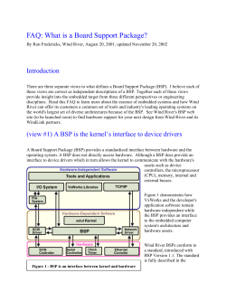


© Copyright 2026