Download Report

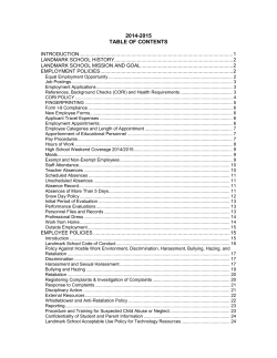
COVER SHEET
Keeratipranon, Narongdech and Maire, Frederic (2005) Bearing Similarity Measures for SelfOrganizing Feature Maps. In Gallagher, Marcus and Hogan, James and Maire, Frederic, Eds.
Proceedings Intelligent Data Engineering and Automated Learning, pages pp. 286-293,
Brisbane Australia.
Accessed from http://eprints.qut.edu.au
Copyright 2005 Springer
Bearing Similarity Measures
for Self-Organizing Feature Maps
Narongdech Keeratipranon and Frederic Maire
Faculty of Information Technology
Queensland University of Technology
Box 2434, Brisbane Q 4001, Australia
[email protected], [email protected]
Abstract. The neural representation of space in rats has inspired many
navigation systems for robots. In particular, Self-Organizing (Feature)
Maps (SOM) are often used to give a sense of location to robots by
mapping sensor information to a low-dimensional grid. For example, a
robot equipped with a panoramic camera can build a 2D SOM from
vectors of landmark bearings. If there are four landmarks in the robot’s
environment, then the 2D SOM is embedded in a 2D manifold lying
in a 4D space. In general, the set of observable sensor vectors form a
low-dimensional Riemannian manifold in a high-dimensional space. In a
landmark bearing sensor space, the manifold can have a large curvature
in some regions (when the robot is near a landmark for example), making the Eulidian distance a very poor approximation of the Riemannian
metric. In this paper, we present and compare three methods for measuring the similarity between vectors of landmark bearings. We also discuss
a method to equip SOM with a good approximation of the Riemannian
metric. Although we illustrate the techniques with a landmark bearing
problem, our approach is applicable to other types of data sets.
1
Introduction
The ability to navigate in an unknown environment is an essential requirement for autonomous mobile robots. Conventional Simultaneous Localization and
Mapping (SLAM) involves fusing observations of landmarks with dead-reckoning
information in order to track the location of the robot and build a map of the
environment [1]. Self Organizing (Feature) Maps (SOM) are capable of representing a robot’s environment. Sensor readings collected at different locations
throughout the environment make up the training set of the SOM. After training, self-localization is based on the association of the the neurons of the SOM
with locations in the environment [2, 3]. Robustness to noise in the sensors can
be achieved with probabilistic methods such as Extended Kalman Filters [4–7]
or Particle Filters [8–10].
Navigation systems based on range sensors such as radar, GPS, laser or ultrasonic sensors are significantly more expensive than navigation systems relying
only on vision [11–13]. An omni-directional vision sensor is composed of a digital
camera aiming at a catadioptric mirror. Although it is not straightforward to
obtain distance estimations from omni-directional images due to the shape of the
mirror, the bearings of landmarks relative to the robot are reasonably accurate
and easy to derive from omni-directional images [14–16].
The Euclidean metric is the default distance used in most neural network
toolboxes. Unfortunately, using this distance to train a SOM on a data-set of
landmark bearing vectors collected at different locations uniformly distributed
throughout the environment does not produce a grid of neurons whose associated
positions in the environment are evenly distributed.
This is not very suprising as the Euclidian distance gives the same importance to all the components of the sensor vectors (here landmark bearings). It is
intuitively clear that is not the right thing to do. The further a landmark is from
the robot the larger the importance of its bearing becomes, as the bearing of a
near landmark changes more wildly than the bearing of a far landmark when
the robot is in motion. Therefore, we should give a relatively large weight to a
far landmark and a relatively small weight to a near landmark. But, what values
should these weights take? How to determine them in practice? In this paper,
we provide answers to those questions.
Section 2 relates three landmark bearing vector metrics to probabilistic classifiers. In the same section, we present numerical experiments comparing these
metrics. Section 3 outlines a method for estimating the intrincic metric of a
Riemannian manifold of sensor inputs. Section 4 concludes this paper.
2
Similarity measures for bearing vectors
In this section, we present three different methods to assess the similarity between two vectors of landmark bearings. The movitation of this project was to
give a robot a sense of location and distance by building a SOM. The input
vectors of the SOM are vectors of landmark bearings. Figure 1 illustrates the
environment of the robot. In this example, the robot roves in a room equipped
with 3 landmarks. The robot collects training sets by performing random walks.
For a 2 × 3 rectangular grid SOM, we could expect that the neurons of a trained
SOM would be uniformely distributed. That is, the neurons should end up at the
centres of the rectangular cells of Figure 1. Experiments with real and simulated
robots show that the SOM fails to spread uniformly (with respect to the ground)
if the Euclidian distance is used in sensor space.
To better understand the causes of the failure of the SOM to spread uniformly, we have investigated the shapes of the cells induced by bearing vector
prototypes corresponding to regularly spaced observations on the ground. Observations were collected throughout the environment of Figure 2. The ground
is partitioned into 15 = 3 × 5 equal size grid cells. The average direction to each
landmark in each cell are represented by the arrows at the centres of the cells.
The length of an arrow represents the importance of the pointed landmark. The
computation of this importance value is explained later in the paper.
l2
l
1
l
3
Fig. 1. A toy model of a robot environment.
The 15 = 3 × 5 mean vectors of landmark bearings in the different cells play
the role of SOM neurons. The corresponding Voronoi diagram computed with
the Euclidian distance on the bearing vectors is shown in Figure 3. We observe
that with the Euclidian distance a large proportion of points get assigned to an
incorrect cell centre. In this context, the localization problem can indeed be cast
as a classification problem. Given a new bearing vector x, determining the cell in
which the observation was made reduces to computing the probabilities P (i|x)
that the obervation has been made in the different rectangular cells i of Figure
2.
A Naive Bayes classifier provides a principled way to assign weights to the
different landmarks. Recall that a Naive Bayes classifier simply makes the assumption that the different features x1 , . . . , x4 of the input vector are conditionally independent with respect to class i. That is, P (x1 , . . . , x4 |i) = P (x1 |i) ×
. . . × P (x4 |i). With this class conditioned independence hypothesis, the most
likely cell i is determined by computing arg i max P (x1 |i) × . . . × P (x4 |i). Let µji
be the mean value of xj observed in cell i, and let σji be the standard deviation
of xj (the bearing of landmark j) observed in cell i. Then, we have
−
1
e
P (xj |i) = √
2πσji
(xj −µji )2
2σ 2
ji
For the classification task, we compute the Naive Bayes pseudo-distance between the input vector x and µi the bearing vector prototype of cell i;
− log(
where θi =
P
j
Y
j
√
log( 2πσji ).
P (xj |i)) =
X (xj − µji )2
+ θi
2
2σji
j
(1)
13
14
15
10
11
12
7
8
9
4
5
6
1
2
3
Fig. 2. An environment partitioned into 15 = 3 × 5 equal size grid cells. The four large
dots are the landmarks.
For this pseudo-distance, the weight of the bearing of a landmark j is determined by the standard deviation of the sample collected in the cell. The right
hand side of Equation 1 is in agreement with our intuition that the further a
landmark j is, the more significant the difference (xj − µji )2 becomes. Indeed
the further the landmark is, the larger 2σ12 is.
ji
Figure 4 shows the Voronoi diagram induced by Naive Bayes pseudo-distance
on landmark bearing vectors is more in agreement with the Euclidian distance
on the ground (compare Figures 3 and 4).
Further improvement in the accuracy of the localization can be obtained
by estimating the covariance matrices of the sensor vector random variable in
the different cells of Figure 2. Let Ci denote the covariance matrix of the ndimensional bearing vectors collected in cell i. The general multivariate Gaussian
density function for a sensor vector x observed in cell i is given by
P (x|i) =
1
n
2
(2π) |Ci |
1
1
2
e− 2 (x−µi )
T
Ci−1 (x−µi )
(2)
The Mahalanobis distance is obtained by taking the negative logarithm of
Equation 2. The Mahalanobis distance has been successfully used for a wide
range of pattern recognition and data mining problems. It has been also extended
to mixed data [17]. In robotics, the Mahalanobis distance has proved useful for
the data association problem [18, 19]. In previous work, the covariance matrix
13
14
15
10
11
12
7
8
9
4
5
6
1
2
3
Fig. 3. Voronoi diagram computed with the Euclidian distance on the bearing vectors.
The induced partition is quite different from the ideal partition of Figure 1. In particular, observation vectors corresponding to points close to the centre of cell 1 are
incorrectly assigned to cell 2.
was used differently. It was used to model the noisy sensors. That is, given the
Cartesian coordinates of the robot and the landmarks, measuments are repeated
(without moving the robot) to estimate the noise in the sensors. Our approach is
fundamentally different. The covariance matrix of the bearing vectors collected in
a given cell i provides us with some information on the geometry of the manifold
around this point in sensor space.
Figure 5 shows the classification results when using the Mahalanobis distance. Our experimental results (in simulation) show that the Euclidean distance achieves a classification accuracy of 92.17% percents, whereas the Naive
Bayes distances achieves a classification accuracy of 97.14% percents. However,
the best results are achieved with the Mahalanobis distance which reaches an
accuracy of 99.32%.
3
Strategy for approximating the Riemannian manifold
It is desirable to automatically build the partition of Figure 2. Unfortunately, a
training set of observations does not allow us to directly compute the covariance
matrices (assuming we have only access to bearing information). Morevover, we
already saw that using a standard SOM training algorithm is not an option
13
14
15
10
11
12
7
8
9
4
5
6
1
2
3
Fig. 4. Voronoi diagram computed with the Naive Bayes classifier weighted distance
on the bearing vectors. About 250 observations per cell were made for the evaluation
of the statistical parameters of the Gaussian distributions.
(failure to spread the neurons evenly with respect to the ground). A possible
strategy is to consider the weighted complete graph G whose vertices are the
bearing vectors of a training set T and whose edge-weigths are the Euclidian
distance between the bearing vectors. Unfortunately, methods that build an
auxiliary graph based on the k-nearest neighbors (like [20]) fail to build a proper
grid for manifolds that have significantly different curvatures in orthogonal directions (the k nearest neighbors will be along the same direction). To address
this problem, we build a graph Gθ obtained from G by removing all edges whose
weights are larger than θ, (or equivalently setting the weights of those edges to
∞). We then compute a grid-like subgraph H of Gθ by imposing constraints
on the relative positions of the neighbors. Preliminary experiments have shown
that it is possible to compute H by simulating annealing using a fitness function
based on the discrepancy of the degrees of the vertices of H (the desired degree
is 4). A suitable representation of H for this search is as a union of a set of
cycles of length 4 of Gθ . From H, we can then estimate the distance between
two bearing vectors on the manifold by computing the length of a shortest path
in H. This work will be presented in a forthcoming paper.
13
14
15
10
11
12
7
8
9
4
5
6
1
2
3
Fig. 5. The best classification is achieved with the Mahalanobis distance.
4
Conclusion
In this paper, we have highligthed the differences between three natural similarity
measures for bearing vectors. We have demonstrated the clear superiority of the
Mahalanobis distance for localization based on bearings problems. We have also
sketched a method for approximating the distance on the Riemannian manifold
defined by a training set of sensor vectors. The approach presented in this paper
is generic and not limited to localization from landmark bearing problems.
References
1. Costa, A., Kantor, G., Choset, H.: Bearing-only landmark initialization with unknown data association. In: Proceedings of the 2004 IEEE International Conference
on Robotics and Automation. Volume 2. (2004) 1764 – 1770
2. Nehmzow, U.: Map Building Through Self-Organisation for Robot Navigation.
1812 edn. Lecture Notes in Computer Science. Springer-Verlag (2000)
3. Gerecke, U., Sharkey, N.E., Sharkey, A.J.C.: Common evidence vectors for selforganized ensemble localization. Neurocomputing 55 (2003) 499–519
4. Smith, R., Self, M., Cheeseman, P.: Estimating uncertain spatial relationships in
robotics. Automous robot vehicles (1990) 167–193
5. Dissanayake, G., Clark, S., Newman, P., Durrant-Whyte, H., Csorba, M.: Estimating uncertain spatial relationships in robotics. IEEE Transactions on Robotics
and Automation 17 (2001) 229 – 241
6. Negenborn, R.: Robot Localization and Kalman Filters. PhD thesis, UTRECHT
UNIVERSITY (2003)
7. Bailey, T.: Constrained initialisation for bearing-only slam. In: Robotics and
Automation IEEE International Conference. Volume 2. (2003) 1966–1971 vol.2
8. Montemerlo, M., Thrun, S.: Fastslam 2.0: An improved particle filtering algorithm
for simultaneous localization and mapping that provably converges. In: Proceedings
of the International Joint Conference on Artifiical Intelligence. (2003)
9. Thrun, S.: Particle filters in robotics. In: Proceedings of the 17th Annual Conference on Uncertainty in AI (UAI). (2002)
10. Fox, D.: Adapting the sample size in particle filters through kld-sampling. The
International Journal of Robotics Research 22 (2003) 985–1003
11. Borenstein, J., Everett, H.R., Feng, L.: Navigating mobile robots: systems and
techniques. Wellesley, Massachusetts: A K. Peters (1996)
12. Garcia-Alegre, M., Garcia-Perez, A.R.L., Martinez, L., Guinea, R., Pozo-Ruz, D.:
An autonomous robot in agriculture tasks. In: 3ECPA-3 European Conf. On Precision Agriculture, France. (2001) 25–30
13. Hanek, R., Schmitt, T.: Vision-based localization and data fusion in a system
of cooperating mobile robots. In: Proceedings of Intelligent Robots and Systems.
(2000)
14. Rizzi, A., Cassinis, R.: robot self-localization system based on omni-directional
color images. In: Robotics and Autonomous Systems 34. (2001) 23–38
15. Yagi, Y., Fujimura, M., Yashida, M.: Route representation for mobile robot navigation by omnidirectional route panorama transformation. In: Proceeding of the
IEEE International Conference on Robotics and Automation, Leuven, Belgium.
(1998)
16. Delahoche, L., Pegard, C., Marhic, B., Vasseur, P.: A navigation system based
on an omni-directional vision sensor. In: Int. Conf. on Intelligent Robotics and
Systems. (1997) 718–724
17. de Leon, A.R., Carriere, K.C.: A generalized mahalanobis distance for mixed data.
Journal of Multivariate Analysis 92 (2005) 174–185
18. Wang, C.C.: Simultaneous Localization, Mapping and Moving Object Tracking.
PhD thesis, Robotics Institute, Carnegie Mellon University, Pittsburgh, PA (2004)
19. Lisien, B., Morales, D., Silver, D., Kantor, G., Rekleitis, I., Choset, H.: Hierarchical simultaneous localization and mapping. In: Intelligent Robots and Systems.
Volume 1. (2003) 448–453
20. Saul, L.K., Roweis, S.T.: Think globally, fit locally: Unsupervised learning of low
dimensional manifolds. Journal of Machine Learning Research 4 (2003) 119–155