1. family and parenting
2. children

Get a Sample for a Discount
Sampling-Based XML Data Pricing
Ruiming Tang1 , Antoine Amarilli2 , Pierre Senellart2 , and St´ephane Bressan1
1
2
National University of Singapore, Singapore
{tangruiming,steph}@nus.edu.sg
Institut Mines–T´el´ecom; T´el´ecom ParisTech; CNRS LTCI. Paris, France
{antoine.amarilli,pierre.senellart}@telecom-paristech.fr
Abstract. While price and data quality should define the major tradeoff for consumers in data markets, prices are usually prescribed by vendors and data quality is not negotiable. In this paper we study a model
where data quality can be traded for a discount. We focus on the case of
XML documents and consider completeness as the quality dimension. In
our setting, the data provider offers an XML document, and sets both
the price of the document and a weight to each node of the document,
depending on its potential worth. The data consumer proposes a price.
If the proposed price is lower than that of the entire document, then
the data consumer receives a sample, i.e., a random rooted subtree of
the document whose selection depends on the discounted price and the
weight of nodes. By requesting several samples, the data consumer can
iteratively explore the data in the document. We show that the uniform
random sampling of a rooted subtree with prescribed weight is unfortunately intractable. However, we are able to identify several practical cases
that are tractable. The first case is uniform random sampling of a rooted
subtree with prescribed size; the second case restricts to binary weights.
For both these practical cases we present polynomial-time algorithms
and explain how they can be integrated into an iterative exploratory
sampling approach.
1
Introduction
There are three kinds of actors in a data market: data consumers, data providers,
and data market owners [14]. A data provider brings data to the market and
sets prices on the data. A data consumer buys data from the market and pays
for it. The owner is the broker between providers and consumers, who negotiates
pricing schemes with data providers and manages transactions to trade data.
In most of the data pricing literature [4–6, 9], data prices are prescribed and
not negotiable, and give access to the best data quality that the provider can
achieve. Yet, data quality is an important axis which should be used to price
documents in data markets. Wang et al. [15, 18] define dimensions to assess data
quality following four categories: intrinsic quality (believability, objectivity, accuracy, reputation), contextual quality (value-added, relevancy, timeliness, ease
of operation, appropriate amount of data, completeness), representational quality (interpretability, ease of understanding, concise representation, consistent
representation), and accessibility quality (accessibility, security).
In this paper, we focus on contextual quality and propose a data pricing
scheme for XML trees such that completeness can be traded for discounted
prices. This is in contrast to our previous work [17] where the accuracy of relational data is traded for discounted prices. Wang et al. [15, 18] define completeness as “the extent to which data includes all the values, or has sufficient
breadth and depth for the current task”. We retain the first part of this definition
as there is no current task defined in our setting. Formally, the data provider
assigns, in addition to a price for the entire document, a weight to each node of
the document, which is a function of the potential worth of this node: a higher
weight is given to nodes that contain information that is more valuable to the
data consumer. We define the completeness of a rooted subtree of the document
as the total weight of its nodes, divided by the total weight of the document.
A data consumer can then offer to buy an XML document for less than the
provider’s set price, but then can only obtain a rooted subtree of the original
document, whose completeness depends on the discount granted.
A data consumer may want to pay less than the price of the entire document
for various reasons: first, she may not be able to afford it due to limited budget
but may be satisfied by a fragment of it; second, she may want to explore the
document and investigate its content and structure before purchasing it fully.
The data market owner negotiates with the data provider a pricing function,
allowing them to decide the price of a rooted subtree, given its completeness
(i.e., the weight). The pricing function should satisfy a number of axioms: the
price should be non-decreasing with the weight, be bounded by the price of the
overall document, and be arbitrage-free when repeated requests are issued by
the same data consumer (arbitrage here refers to the possibility to strategize the
purchase of data). Hence, given a proposed price by a data consumer, the inverse
of the pricing function decides the completeness of the sample that should be
returned. To be fair to the data consumer, there should be an equal chance to
explore every possible part of the XML document that is worth the proposed
price. Based on this intuition, we sample a rooted subtree of the XML document
of a certain weight, according to the proposed price, uniformly at random.
The data consumer may also issue repeated requests as she is interested in
this XML document and wants to explore more information inside in an iterative
manner. For each repeated request, a new rooted subtree is returned. A principle
here is that the information (document nodes) already paid for should not be
charged again. Thus, in this scenario, we sample a rooted subtree of the XML
document of a certain weight uniformly at random, without counting the weight
of the nodes already bought in previously issued requests.
The present article brings the following contributions:
– We propose to realize the trade-off between quality and discount in data
markets. We propose a framework for pricing the completeness of XML data,
based on uniform sampling of rooted subtrees in weighted XML documents.
(Section 3)
– We show that the general uniform sampling problem in weighted XML trees
is intractable. In this light, we propose two restrictions: sampling based on
the number of nodes, and sampling when weights are binary (i.e., weights
are 0 or 1). (Section 4)
– We show that both restrictions are tractable by presenting a polynomialtime algorithm for uniform sampling based on the size of a rooted subtree,
or on 0/1-weights. (Section 5)
– We extend our framework to the case of repeated sampling requests where
the data consumer is not charged twice the same nodes. Again, we obtain
tractability when the weight of a subtree is its size. (Section 6)
2
Related Work
Data Pricing. The basic structure of data markets and different pricing schemes
were introduced in [14]. The notion of “query-based” pricing was introduced in [4,
6] to define the price of a query as the price of the cheapest set of pre-defined
views that can determine the query. It makes data pricing more flexible, and
serves as the foundation of a practical data pricing system [5]. The price of
aggregate queries has been studied in [9]. Different pricing schemes are investigated and multiple pricing functions are proposed to avoid several pre-defined
arbitrage situations in [10]. However, none of the works above takes data quality
into account, and those works do not allow the data consumer to propose a price
less than that of the data provider, which is the approach that we study here.
The idea of trading off price for data quality has been explored in the context
of privacy in [8], which proposes a theoretic framework to assign prices to noisy
query answers. If a data consumer cannot afford the price of a query, she can
choose to tolerate a higher standard deviation to lower the price. However, this
work studies pricing on accuracy for linear relational queries, rather than pricing
XML data on completeness. In [17], we propose a relational data pricing framework in which data accuracy can be traded for discounted prices. By contrast,
this paper studies pricing for XML data, and proposes a tradeoff based on data
completeness rather than accuracy.
Subtree/Subgraph Sampling. The main technical result of this paper is the
tractability of uniform subtree sampling under a certain requested size. This
question is related to the general topic of subtree and subgraph sampling, but,
to our knowledge, it has not yet been adequately addressed.
Subgraph sampling works such as [3, 7, 13, 16] have proposed algorithms to
sample small subgraphs from an original graph while attempting to preserve
selected metrics and properties such as degree distribution, component distribution, average clustering coefficient and community structure. However, the
distribution from which these random graphs are sampled is not known and
cannot be guaranteed to be uniform.
Other works have studied the problem of uniform sampling [2, 11]. However,
[2] does not propose a way to fix the size of the samples. The authors of [11]
propose a sampling algorithm to sample a connected sub-graph of size k under
an approximately uniform distribution; note that this work provides no bound
on the error relative to the uniform distribution.
Sampling approaches are used in [19, 12] to estimate the selectivity of XML
queries (containment join and twig queries, respectively). Nevertheless, the samples in [19] are specific to containment join queries, while those in [12] are representatives of the XML document for any twig queries. Neither of those works
controls the distribution from which the subtrees are sampled.
In [1], Cohen and Kimelfeld show how to evaluate a deterministic tree automaton on a probabilistic XML document, with applications to sampling possible worlds that satisfy a given constraint, e.g., expressed in monadic second-order
logic and then translated into a tree automaton. Note that the translation of constraints to tree automata itself is not tractable; in this respect, our approach can
be seen as a specialization of [1] to the simpler case of fixed-size or fixed-weight
tree sampling, and as an application of it to data pricing.
3
Pricing Function and Sampling Problem
This paper studies data pricing for tree-shaped documents. Let us first formally
define the terminology that we use for such documents.
We consider trees that are unordered, directed, rooted, and weighted. Formally, a tree t consists of a set of nodes V(t) (which are assumed to carry unique
identifiers), a set of edges E(t), and a function w mapping every node n ∈ V(t)
to a non-negative rational number w(n) which is the weight of node n. We
write root(t) for the root node of t. Any two nodes n1 , n2 ∈ V(t) such that
(n1 , n2 ) ∈ E(t) are in a parent-child relationship, that is, n1 is the parent of n2
and n2 is a child of n1 .
By children(n), we represent the set of nodes that have parent n. A tree is
said to be binary if each node of the tree has at most two children, otherwise it
is unranked. Throughout this paper, for ease of presentation, we may call such
trees “XML documents”.
We now introduce the notion of rooted subtree of an XML document:
Definition 1. (Subtree, rooted subtree) A tree t0 is a subtree of a tree t if
V(t0 ) ⊆ V(t) and E(t0 ) ⊆ E(t). A rooted subtree t0 of a tree t is a subtree
of t such that root(t) = root(t0 ). We name it r-subtree for short. The weight
function for a subtree t0 of a tree t is always assumed to be the restriction of the
weight function for t on the nodes in t0 .
For technical reasons, we also sometimes talk of the empty subtree that contains no node.
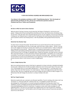
Example 1. Figure 1 presents two example trees. The nodes {n0 , n2 , n5 }, along
with the edges connecting them, form an r-subtree of the tree in Figure 1(a).
n0
n0
n1
n0
n2
n1
n4
(a) A tree
n5
n1
n6
n4
n2
n3
n2
n3
n2
n5
n4
n1
n3
n0
n5
(b) A binary tree
Fig. 1. Two example trees (usage of the square node will be introduced in Section 5.2)
Likewise, the nodes {n2 , n4 , n5 } and the appropriate edges form a subtree of that
tree (but not an r-subtree). The tree of Figure 1(b) is a binary tree (ignore the
different shapes of the nodes for now).
t
u
We now present our notion of data quality, by defining the completeness of
an r-subtree, based on the weight function of the original tree:
Definition 2. (Weight
P of a tree) For a node n ∈ V(t), we define inductively
weight(n) = w(n) + (n,n0 )∈E(t) weight(n0 ). With slight abuse of notation, we
note weight(t) = weight(root(t)) as the weight of t.
Definition 3. (Completeness of an r-subtree) Let t be a tree. Let t0 be an r0
)
subtree of t. The completeness of t0 with respect to t is ct (t0 ) = weight(t
weight(t) . It is
0
obvious that ct (t ) ∈ [0, 1].
We study a framework for data markets where the data consumer can buy
an incomplete document from the data provider while paying a discounted price.
The formal presentation of this framework consists of three parts:
1. An XML document t.
2. A pricing function ϕt for t whose input is the desired completeness for an rsubtree of the XML document, and whose value is the price of this r-subtree.
Hence, given a proposed price pr0 by a data consumer, the completeness of
the returned r-subtree is decided by ϕ−1
t (pr0 ).
3. An algorithm to sample an r-subtree of the XML document uniformly at
random among those of a given completeness.
We study the question of the sampling algorithm more in detail in subsequent sections. For now, we focus on the pricing function, starting with a formal
definition:
Definition 4. (Pricing function) The pricing function for a tree t is a function ϕt : [0, 1] → Q+ . Its input is the completeness of an r-subtree t0 and it
returns the price of t0 , as a non-negative rational.
n4
n3
n5
n6
A healthy data market should impose some restrictions on ϕt , such as:
Non-decreasing. The more complete an r-subtree is, the more expensive it
should be, i.e., c1 > c2 ⇒ ϕt (c1 ) > ϕt (c2 ).
Arbitrage-free. Buying an r-subtree of completeness c1 + c2 should not be
more expensive than buying two subtrees with respective completeness c1
and c2 , i.e., ϕt (c1 ) + ϕt (c2 ) > ϕt (c1 + c2 ). In other words, ϕt should be subadditive. This property is useful when considering repeated requests, studied
in Section 6.
Minimum and maximum bound. We should have ϕt (0) = prmin and ϕt (1) =
prt , where prmin is the minimum cost that a data consumer has to pay using
the data market and prt is the price of the whole tree t. Note that by the
non-decreasing character of ϕt , prt > prmin > 0.
All these properties can be satisfied, for instance, by functions of the form
ϕt (c) = (prt − prmin )cp + prmin where p 6 1; however, if p > 1, the arbitrage-free
property is violated.
Given a proposed price pr0 by a data consumer, ϕ−1
t (pr0 ) is the set of possible
corresponding completeness values. Note that ϕ−1
is a relation and may not
t
be a function; ϕ−1
is
a
function
if
different
completeness
values correspond to
t
different prices. Once a completeness value c ∈ ϕ−1
(pr
)
is
chosen, the weight
0
t
of the returned r-subtree is fixed as c × weight(t).
Therefore, in the rest of the paper, we consider the problem of uniform sampling an r-subtree with prescribed weight (instead with prescribed completeness).
Let us now define the problem that should be solved by our sampling algorithm:
Definition 5. (Sampling problem) The problem of sampling an r-subtree,
given a tree t and a weight k, is to sample an r-subtree t0 of t, such that
weight(t0 ) = k, uniformly at random, if one exists, or fail if no such r-subtree
exists.
4
4.1
Tractability
Intractability of the Sampling Problem
We now turn to the question of designing an algorithm to solve the sampling
problem defined in the previous section. Sadly, it can be shown that this problem
is already NP-hard in the general formulation that we gave.
Proposition 1. Given a tree t and a weight x, it is NP-hard to sample an
r-subtree of t of weight x uniformly at random.
Proof. Consider the simpler problem of deciding if such an r-subtree of t exists.
Further restrict t such that w(n) = 0 unless n is a leaf. In this case, deciding
whether there exists an r-subtree of weight x is equivalent to the subset-sum
problem, which is known to be NP-complete. Now there is a PTIME-reduction
from this existence problem to the sampling problem, as an algorithm for sampling can be used to decide whether there exists an r-subtree of the desired
weight (the algorithm returns one such) or if none exists (the algorithm fails).
t
u
4.2
Tractable Cases
We now define restricted variants of the sampling problem where the weight
function is assumed to be of a certain form. In the next section, we show that
sampling for these variants can be performed in PTIME.
Unweighted Sampling. In this setting, we take the weight function w(n) = 1
for all n ∈ V(t). Hence, the weight of a tree t is actually the number of nodes in
t, i.e., its size, which we write size(t).
In this case, the hardness result of Proposition 1 does not apply anymore.
However, sampling an r-subtree with prescribed size uniformly at random is still
not obvious to do, as the following example shows:
Example 2. Consider the problem of sampling an r-subtree t0 of size 3 from
the tree t in Figure 1(a). We can enumerate all such r-subtrees: {n0 , n1 , n2 },
{n0 , n1 , n3 }, {n0 , n2 , n3 }, {n0 , n2 , n4 } and {n0 , n2 , n5 }, and choose one of them
at random with probability 51 . However, as the number of r-subtrees may be
exponential in the size of the document in general, we cannot hope to perform
this approach in PTIME. Observe that it is not easy to build a random r-subtree
node by node: it is clear that node n0 must be included, but then observe that
we cannot decide to include n1 , n2 , or n3 , uniformly at random. Indeed, if we
do this, our distribution on the r-subtrees will be skewed, as n1 (or n3 ) occurs
in 52 of the outcomes whereas n2 occurs in 54 of them. Intuitively, this is because
there are more ways to choose the next nodes when n2 is added, than when n1
or n3 are added.
t
u
We show in the next section that this problem can be solved in PTIME.
0/1-weights Sampling. In this more general problem variant, we require that
w(n) ∈ {0, 1} for all n ∈ V(t), i.e., the weight is binary.
We show in Section 5.3 that this problem can also be solved in PTIME using
an adaptation of the unweighted sampling algorithm.
5
Algorithms for Tractable Uniform Sampling
In this section, we present a PTIME algorithm for the unweighted sampling
problem, namely the problem of sampling an r-subtree of size k from an XML
document, uniformly at random.
We first describe the algorithm for the case of binary trees, in Section 5.1.
Next, we adapt the algorithm in Section 5.2 to show how to apply it to arbitrary
trees. Last, we study the more general case of 0/1-weights in Section 5.3, showing
that the algorithm for unweighted sampling can be adapted to solve this problem.
Algorithm 1: Algorithm for unweighted sampling problem on binary trees
1
2
3
4
5
Input: a binary tree t and an integer k > 0
Result: an r-subtree t0 of t of size(t0 ) = k uniformly at random
// Phase 1: count the number of subtrees
D ← SubtreeCounting(t);
// Phase 2: sample a random subtree
if k 6 size(t) then
return UniformSampling(root(t), D, k);
else
fail;
Algorithm 2: SubtreeCounting(t)
Input: a binary tree t
Result: a matrix D such that Di [k] is the number of r-subtrees of size k rooted
at ni for all i and k
9
DNULL [0] ← 1;
// We browse all nodes in topological order
foreach non-NULL node ni accessed bottom-up do
nj ← first child of ni (or NULL if none exists);
ng ← second child of ni (or NULL if none exists);
Di [0] ← 1;
T ← Dj ⊕ Dg ;
for j ∈ [0, |T | − 1] do
Di [j + 1] ← T [j];
return D;
5.1
Unweighted Sampling for Binary Trees
1
2
3
4
5
6
7
8
In this section, we provide an algorithm which proves the following theorem:
Theorem 1. The unweighted sampling problem for binary trees can be solved
in PTIME.
Our general algorithm to solve this problem is given as Algorithm 1. The
algorithm has two phases, which we study separately in what follows. For simplicity, whenever we discuss binary trees in this section, we will add special NULL
children to every node of the tree (except NULL nodes themselves), so that all
nodes, including leaf nodes, have exactly two children (which may be NULL).
This will simplify the presentation of the algorithms.
First phase: Subtree Counting (Algorithm 2). We start by computing
a matrix D such that, for every node ni of the input tree t and any value
0 6 k 6 size(t), Di [k] is the number of subtrees of size k rooted at node ni . We
do so with Algorithm 2 which we now explain in detail.
There is only one subtree rooted at the special NULL node, namely the empty
subtree, with size 0, which provides the base case of the algorithm (line 1). Otherwise, we compute Di for a node ni from the values Dj and Dg of D for its children nj and ng (which may be NULL); those values have been computed before
because nodes are considered following a topological ordering, in a bottom-up
fashion.
Intuitively, the only r-subtree of size 0 is the empty subtree, hence we must
have Di [0] = 1 (line 5). Otherwise, any r-subtree of size k > 0 rooted at ni
is obtained by retaining ni , and choosing two r-subtrees tj and tg , respectively
rooted at nj and ng (the children of ni ), such that size(tj ) + size(tg ) = k − 1
(which accounts for the size of the additional node ni ). The number of such
choices is computed by the convolution of Dj and Dg in line 6, defined as:
min(p,|Dj |−1)
For 0 6 p 6 |Dj |+|Dg |−2,
(Dj ⊕Dg )[p] :=
X
Dj [m]×Dg [p−m].
m=max(0,p−|Dg |−1)
Lines 7 and 8 account for the size of the retained node ni .
Example 3. Let t be the tree presented in Figure 1(b) (again, ignore the different
shapes of nodes for now). Starting from the leaf nodes, we compute D1 = D4 =
D5 = D3 = (1, 1), applying lines 5 to 8 on DNULL ⊕ DNULL = (1). This means
that there are two r-subtrees rooted at leaf nodes: the empty subtree, and the
subtree with just that leaf.
Now, when computing D2 , we first convolve D4 and D5 to get the numbers of
pairs of r-subtrees of different sizes at {n4 , n5 }, i.e., D4 ⊕ D5 = (1, 2, 1), so that
D2 = (1, 1, 2, 1). When computing D6 , we first compute D2 ⊕ D3 = (1, 2, 3, 3, 1),
so that D6 = (1, 1, 2, 3, 3, 1). Finally, D0 = (1, 1, 2, 3, 5, 6, 4, 1).
t
u
We now state the correctness and running time of this algorithm.
Lemma 1. Algorithm 2 terminates in time polynomial in size(t) and returns D
such that, for every i and k, Di [k] is the number of r-subtrees of size k rooted at
node ni .
Proof. Let us first prove the running time. All arrays under consideration have
size at most n (n = size(t)), so computing the convolution sum of two such arrays
is in time O(n2 ) (computing each value of the convolution sum is in time O(n)).
The number of convolution sums to compute overall is O(n), because each array
Di occurs in exactly one convolution sum. The overall running time is O(n3 ).
Let us now show correctness. We proceed by induction on the node ni to
prove the claim for every k. The base case is the NULL node, whose correctness
is straightforward. Let us prove the induction step. Let ni be a node, and assume
by induction that Dj [k 0 ] is correct for every k 0 for every child nj of ni . Let us fix
k and show that Di [k] is correct. To select an r-subtree at ni , either k = 0 and
there is exactly one possibility (the empty subtree), or k > 0 and the number
of possibilities is the number of ways to select a set of r-subtrees at the children
of ni so that their size sum to k − 1. This is the role of lines 5 to 8. Now, to
Algorithm 3: UniformSampling(ni , D, x)
Input: a node ni (or NULL), the precomputed D, and a size value x
Result: an r-subtree of size x at node ni
1
2
3
4
5
6
7
8
9
10
if x = 0 then
return ∅;
nj ← first child of ni (or NULL if none exists);
ng ← second child of ni (or NULL if none exists);
for 0 6 sj 6 size(nj ), 0 6 sg 6 size(ng ) s.t. sj + sg = x − 1 do
p(sj , sg ) ← Dj [sj ] × Dg [sg ];
P
Sample an (sj , sg ) with probability p(sj , sg ) normalized by sj ,sg p(sj , sg );
L ← UniformSampling(nj , D, sj );
R ← UniformSampling(ng , D, sg );
return the tree rooted at ni with child subtrees L and R;
enumerate the ways of choosing r-subtrees at children of ni whose size sum to
k −1, we can first decide the size of the selected r-subtree for each child: the ways
to assign such sizes form a partition of the possible outcomes, so the number
of outcomes is the sum, over all such assignments of r-subtree sizes to children,
of the number of outcomes for this assignment. Now, for a fixed assignment,
the subtrees rooted at each children are chosen independently, so the number of
outcomes for a fixed assignment is the product of the number of outcomes for
the given size for each child, which by induction hypothesis is correctly reflected
by the corresponding Dj [k 0 ]. Hence, for a given k, either k = 0, or k > 0, in
which case Di [k] is (Dj ⊕ Dg )[k − 1] by lines 5 to 8, which sums, over all possible
subtree size assignments, the number of choices for this subtree size assignment.
Hence, by induction, we have shown the desired claim.
t
u
Second phase: Uniform Sampling (Algorithm 3). In the second phase of
Algorithm 1, we sample an r-subtree from t in a recursive top-down manner,
based on the matrix D computed by Algorithm 2. Our algorithm to perform
this uniform sampling is Algorithm 3. The basic idea is that to sample an rsubtree rooted at a node ni , we decide on the size of the subtrees rooted at each
child node, biased by the number of outcomes as counted in D, and then sample
r-subtrees of the desired size recursively.
Let us now explain Algorithm 3 in detail.
If x = 0, we must return the empty tree (lines 1 and 2). Otherwise we return
ni and subtrees tj and tg rooted at the children nj and ng of ni . We first decide
on the size sj and sg of tj and tg (lines 5 to 7) before sampling recursively a
subtree of the prescribed size, uniformly at random, and returning it.
The possible size pairs (sj , sg ) must satisfy the following conditions to be
possible choices for the sizes of the subtrees tj and tg :
1. 0 6 sj 6 size(nj ) and 0 6 sg 6 size(ng ) (of course size(NULL) = 0)
2. sj + sg = x − 1 (which accounts for node ni )
Intuitively, to perform a uniform sampling, we now observe that the choice of
the size pair (sj , sg ) partitions the set of outcomes. Hence, the probability that
we select one size pair should be proportional to the number of possible outcomes
for this pair, namely, the number of r-subtrees tj and tg such that size(tj ) = sj
and size(tg ) = sg . We compute this from Dj and Dg (line 6) by observing that
the number of pairs (tj , tg ) is the product of the number of choices for tj and
for tg , as every combination of choices is possible.
Example 4. Follow Example 3. Assume we want to sample an r-subtree t0 of
size(t0 ) = 3 uniformly. We first call UniformSampling(n0 , 3). We have to return
n0 . Now n0 has two children, n1 and n6 . The possible size pairs are (0, 2) and
(1, 1), with respective (unnormalized) probabilities p(0, 2) = D1 [0] × D6 [2] =
1 × 2 = 2 and p(1, 1) = D1 [1] × D6 [1] = 1 × 1 = 1. The normalized probabilities
are therefore 32 and 13 . Assume that we choose (0, 2). We now call recursively
UniformSampling(n1 , 0) and UniformSampling(n6 , 2).
UniformSampling(n1 , 0) returns ∅. We proceed to UniformSampling(n6 , 2). We
have to return n6 . Now n6 has two children, n2 and n3 . The possible size pairs for
this call are (1, 0) and (0, 1) with probabilities 21 and 12 . Assume that we choose
(1, 0). We now call recursively UniformSampling(n2 , 1) and UniformSampling(n3 , 0).
UniformSampling(n3 , 0) returns ∅. We proceed to UniformSampling(n2 , 1). n2
is selected. n2 has two children, n4 and n5 . There is only one possible size
pair for this call (0, 0) with probability 1. We can only choose (0, 0) and call
UniformSampling(n4 , 0) (which results in ∅) and UniformSampling(n5 , 0) (which
results in ∅). Hence, the end result is the r-subtree whose nodes are {n0 , n6 , n2 }
(and whose edges can clearly be reconstituted in PTIME from t).
t
u
We now show the tractability and correctness of Algorithm 3.
Lemma 2. For any tree t, node ni ∈ V(t) and integer 0 6 x 6 size(ni ), given
D computed by Algorithm 2, UniformSampling(ni , D, x) terminates in polynomial
time and returns an r-subtree of size x rooted at ni , uniformly at random (i.e.,
solves the unweighted sampling problem for binary trees).
Proof. Let us first prove the complexity claim. On every node ni of the binary
tree t, the number of possibilities to consider is linear in the tree size because
every node has exactly two children, and for each possibility the number of
operations performed is constant (assuming that drawing a number uniformly at
random is constant-time). The overall running time is quadratic, i.e., O(size(t)2 ).
We now show correctness by induction on ni . The base case is ni = NULL,
in which case we must have x = 0 and we correctly return ∅. Otherwise, if
ni is not NULL, either x = 0 and we correctly return ∅, or x > 0 and, as in
the proof of Lemma 1, the set of possible outcomes of the sampling process is
partitioned by the possible assignments, and only the valid ones correspond to
a non-empty set of outcomes. Hence, we can first choose a size pair, weighted by
the proportion of outcomes which are outcomes for that assignment, and then
choose an outcome for this pair. Now, observe that, by Lemma 1, D correctly
represents the number of outcomes for each child of ni , so that our computation
of p (which mimics that of Algorithm 2) correctly represents the proportion of
outcomes that are outcomes for every size pair. We then choose an assignment
according to p, and then observe that choosing an outcome for this assignment
amounts to choosing an outcome for each child of ni whose size is given by the
assignment. By induction hypothesis, this is precisely what the recursive calls to
UniformSampling(ni , D, x) perform. This concludes the proof.
t
u
5.2
Algorithm for Sampling an Unranked Tree
In this section, we show that the algorithm of the previous section can be adapted
so that it works on arbitrary unranked trees, not just binary trees.
We first observe that the straightforward generalization of Algorithm 1 to
trees of arbitrary arity, where assignments and convolutions are performed for all
children, is still correct. However, it would not run in polynomial time anymore
as there would be a potentially exponential number of size pairs to consider.
Fortunately, there is still hope to avoid enumerating the size pairs over all the
children, thanks to the associativity of convolution sum. Informally, assume we
have three children {n1 , n2 , n3 }, we do the following: we treat {n1 } as a group and
{n2 , n3 } as the second group, then enumerate size pairs over {n1 } and {n2 , n3 };
once a size pair, in which a positive integer is assigned to {n2 , n3 }, is selected,
we can treat {n2 } and {n3 } as new groups and enumerate size pairs over {n2 }
and {n3 }. This strategy can be implemented by transforming the original tree
to a binary tree. From this intuition, we now state our result:
Theorem 2. The unweighted sampling problem can be solved in PTIME, for
arbitrary unranked trees.
Proof (Sketch). The proof proceeds by encoding arbitrary trees to encoded trees,
that are binary trees whose nodes are either regular nodes or dummy nodes.
Intuitively, the encoding operation replaces sequences of more than two children
by a hierarchy of dummy nodes representing those children; replacing dummy
nodes by the sequence of their children yields back the original tree. The encoding
is illustrated in Figure 1, where the tree in Figure 1(b) is the encoded tree of
the one in Figure 1(a) (dummy nodes are represented as squares).
It can then be shown that, up to the question of keeping or deleting the
dummy nodes with no regular descendants (we call them bottommost), there is
a bijection between r-subtrees in the original tree and r-subtrees in the encoded
tree. Hence, we can solve the unweighted sampling problem by choosing an rsubtree in the encoded tree with the right number of regular nodes, uniformly
at random, and imposing the choice of keeping bottommost dummy nodes.
There only remains to adapt Algorithms 2 and 3 to run correctly on encoded
trees, that is, mananging dummy nodes correctly.
We change Algorithm 2 by replacing lines 5 to 8 with Di ← Dj ⊕ Dg when
ni is a dummy node (as it must always be kept, and does not increase the size
of the r-subtree).
We change Algorithm 3 by imposing at line 1 the condition that ni is either
NULL or a regular node (otherwise we cannot return ∅ as we must keep dummy
nodes). Also, we change line 5 so that, when node ni is a dummy node, we
require sj + sg = x (rather than x − 1), as we do not count the dummy node in
the size of the resulting subtree.
The correctness and running time of the modified algorithms can be proved
by straightforward adaptations of Lemma 1 and Lemma 2.
t
u
5.3
Uniform Sampling under 0/1-weights
Our tractability result extends to trees with binary weights:
Theorem 3. The 0/1-weights sampling problem can be solved in PTIME, for
arbitrary unranked trees.
Proof (Sketch). The proof proceeds by modifying the unweighted sampling algorithm to handle nodes of weight 0 (in addition to the modifications described
in the previous section).
In Algorithm 2, when ni is a weight-0 node, lines 7 to 8 must be replaced by
j ∈ [1, |T | − 1], Di [j] ← T [j] (the node has no weight); line 5 is removed and set
Di [0] ← 1 + T [0] (we can keep or discard the weight-0 node, unlike the dummy
nodes of the previous section).
In Algorithm 3, when x = 0 and ni is a weight-0 node, the empty subtree
should be returned with probability Di1[0] ; otherwise, continue the execution of
the algorithm to return a random non-empty r-subtree of size 0. This is because
the introduction of weight-0 nodes, unlike weight-1 and dummy nodes, leads to
multiple ways to sample a r-subtree of size 0. If ni is a weight-0 node, line 5
should be changed to require sj + sg = x rather than x − 1, as for dummy nodes.
The correctness and running time of the modified algorithms can be proved
by straightforward adaptations of Lemmas 1 and 2.
t
u
6
Repeated Requests
In this section, we consider the more general problem where the data consumer
requests a completion of a certain price to data that they have already bought.
The motivation is that, after having bought incomplete data, the user may realize
that they need additional data, in which case they would like to obtain more
incomplete data that is not redundant with what they already have.
A first way to formalize the problem is as follows, where data is priced according to a known subtree (provided by the data consumer) by considering that
known nodes are free (but that they may or may not be returned again).
Definition 6. The problem of sampling an r-subtree of weight k in a tree t
conditionally to an r-subtree t0 P
is to sample an r-subtree t00 of t uniformly at
00
random, such that weight(t ) − n∈(V(t0 )∩V(t00 )) w(n) = k.
An alternative is to consider that we want to sample an extension of a fixed
size to the whole subtree, so that all known nodes are part of the output:
Definition 7. The problem of sampling an r-subtree of weight k in a tree t that
extends an r-subtree t0 is to sample an r-subtree t00 of t uniformly at random,
such that (1) t0 is an r-subtree of t00 ; (2) weight(t00 ) − weight(t0 ) = k.
Note that those two formulations are not the same: the first one does not
require the known part of the document to be returned, while the second one
does. While it may be argued that the resulting outcomes are essentially equivalent (as they only differ on parts of the data that are already known to the data
consumer), it is important to observe that they define different distributions:
though both problems require the sampling to be uniform among their set of
outcomes, the additional possible outcomes of the first definition means that the
underlying distribution is not the same.
As the uniform sampling problem for r-subtrees can be reduced to either problem by setting t0 to be the empty subtree, the NP-hardness of those two problems
follows from Proposition 1. However, we can show that, in the unweighted case,
those problems are tractable, because they reduce to the 0/1-weights sampling
problem which is tractable by Theorem 3:
Proposition 2. The problem of sampling an r-subtree of weight k in a tree t
conditionally to an r-subtree t0 can be solved in PTIME if t is unweighted. The
same holds for the problem of sampling that extends another r-subtree.
Proof (Sketch). For the problem of Definition 6, set the weight of the nodes of t0
in t to be zero (the intuition is that all the known nodes are free). The problem
can then be solved by applying Theorem 3.
For the problem of Definition 7, set the weight of the nodes of t0 in t to be
zero but we have to ensure that weight-0 nodes are always returned. To do so,
we adapt Theorem 3 by handling weight-0 nodes in the same way as handling
dummy nodes in the previous section.
t
u
7
Conclusion
We proposed a framework for a data market in which data quality can be traded
for a discount. We studied the case of XML documents with completeness as
the quality dimension. Namely, a data provider offers an XML document, and
sets both the price and weights of nodes of the document. The data consumer
proposes a price but may get only a sample if the proposed price is lower than
that of the entire document. A sample is a rooted subtree of prescribed weight,
as determined by the proposed price, sampled uniformly at random.
We proved that if nodes in the XML document have arbitrary non-negative
weights, the sampling problem is intractable. We identified tractable cases, namely
the unweighted sampling problem and 0/1-weights sampling problem, for which
we devised PTIME algorithms. We proved the time complexity and correctness
of the algorithms. We also considered repeated requests and provided PTIME
solutions to the unweighted cases.
The more general issue that we are currently investigating is that of sampling
rooted subtrees uniformly at random under more expressive conditions than size
restrictions or 0/1-weights. In particular, we intend to identify the tractability
boundary to describe the class of tree statistics for which it is possible to sample
r-subtrees in PTIME under a uniform distribution.
Acknowledgment. This work is supported by the French Ministry of European and Foreign Affairs under the STIC-Asia program, CCIPX project.
References
1. S. Cohen, B. Kimelfeld, and Y. Sagiv. Running tree automata on probabilistic
XML. In PODS, pages 227–236, 2009.
2. M. R. Henzinger, A. Heydon, M. Mitzenmacher, and M. Najork. On near-uniform
URL sampling. Computer Networks, 33(1-6), 2000.
3. C. H¨
ubler, H.-P. Kriegel, K. Borgwardt, and Z. Ghahramani. Metropolis algorithms
for representative subgraph sampling. In ICDM, 2008.
4. P. Koutris, P. Upadhyaya, M. Balazinska, B. Howe, and D. Suciu. Query-based
data pricing. In PODS, 2012.
5. P. Koutris, P. Upadhyaya, M. Balazinska, B. Howe, and D. Suciu. QueryMarket
demonstration: Pricing for online data markets. PVLDB, 5(12), 2012.
6. P. Koutris, P. Upadhyaya, M. Balazinska, B. Howe, and D. Suciu. Toward practical
query pricing with QueryMarket. In SIGMOD, 2013.
7. J. Leskovec and C. Faloutsos. Sampling from large graphs. In SIGKDD, 2006.
8. C. Li, D. Y. Li, G. Miklau, and D. Suciu. A theory of pricing private data. In
ICDT, 2013.
9. C. Li and G. Miklau. Pricing aggregate queries in a data marketplace. In WebDB,
2012.
10. B.-R. Lin and D. Kifer. On arbitrage-free pricing for general data queries. PVLDB,
7(9):757–768, 2014.
11. X. Lu and S. Bressan. Sampling connected induced subgraphs uniformly at random. In SSDBM, 2012.
12. C. Luo, Z. Jiang, W.-C. Hou, F. Yu, and Q. Zhu. A sampling approach for XML
query selectivity estimation. In EDBT, 2009.
13. A. S. Maiya and T. Y. Berger-Wolf. Sampling community structure. In WWW,
2010.
14. A. Muschalle, F. Stahl, A. Loser, and G. Vossen. Pricing approaches for data
markets. In BIRTE, 2012.
15. L. Pipino, Y. W. Lee, and R. Y. Wang. Data quality assessment. Commun. ACM,
45(4), 2002.
16. B. F. Ribeiro and D. F. Towsley. Estimating and sampling graphs with multidimensional random walks. In Internet Measurement Conference, 2010.
17. R. Tang, D. Shao, S. Bressan, and P. Valduriez. What you pay for is what you
get. In DEXA (2), 2013.
18. R. Y. Wang and D. M. Strong. Beyond accuracy: What data quality means to
data consumers. J. of Management Information Systems, 12(4), 1996.
19. W. Wang, H. Jiang, H. Lu, and J. X. Yu. Containment join size estimation: Models
and methods. In SIGMOD, 2003.