Sample Size Calculations
…
or the Myth of Power
…or
π
ε
χ
ε
π Pharma Edge
Helmut Schütz
BEBAC
Biostatistics:
Biostatistics: Basic concepts & applicable principles for various designs
in bioequivalence studies and data analysis | Mumbai,
Mumbai, 29 – 30 January 2011
Attribution--ShareAlike 3.0 Unported
Wikimedia Commons • 2007 Sujit Kumar • Creative Commons Attribution
Sample Size Calculations …or the Myth of Power
1 • 49
Sample Size Calculations …or the Myth of Power
Sample Size (Limits)
Minimum
12:
π
ε
χ
ε
π Pharma Edge
WHO, EU, CAN, NZ, AUS, AR, MZ, ASEAN States,
RSA
12: USA ‘A pilot study that documents BE can be
appropriate, provided its design and execution are
suitable and a sufficient number of subjects (e.g.,
12) have completed the study.’
20: RSA (MR formulations)
24: Saudia Arabia (12 to 24 if statistically justifiable)
24: Brazil
Sufficient number: JPN
Biostatistics:
Biostatistics: Basic concepts & applicable principles for various designs
in bioequivalence studies and data analysis | Mumbai,
Mumbai, 29 – 30 January 2011
2 • 49
Sample Size Calculations …or the Myth of Power
Sample Size (Limits)
Maximum
NZ: ‘If the calculated number of subjects appears to be
higher than is ethically justifiable, it may be
necessary to accept a statistical power which is
less than desirable. Normally it is not practical to
use more than about 40 subjects in a bioavailability
study.’
All others: Not specified (judged by IEC/IRB or local
Authorities).
ICH E9, Section 3.5 applies: ‘The number of
subjects in a clinical trial should always be large
enough to provide a reliable answer to the
questions addressed.’
π
ε
χ
ε
π Pharma Edge
Biostatistics:
Biostatistics: Basic concepts & applicable principles for various designs
in bioequivalence studies and data analysis | Mumbai,
Mumbai, 29 – 30 January 2011
3 • 49
Sample Size Calculations …or the Myth of Power
Power & Sample Size
Reminder
Generally power is set to at least 80% (β, error type II:
producers’s risk to get no approval for a bioequivalent
formulation; power = 1 – β).
1 out of 5 studies will fail just by chance!
If you plan for power of less than 70%, problems with the
ethics committee are likely (ICH E9).
If you plan for power of more than 90% (especially with
low variability drugs), problems with the regulator are
possible (‘forced bioequivalence’).
Add subjects (‘alternates’) according to the expected
drop-out rate – especially for studies with more than two
periods or multiple-dose studies.
π
ε
χ
ε
π Pharma Edge
Biostatistics:
Biostatistics: Basic concepts & applicable principles for various designs
in bioequivalence studies and data analysis | Mumbai,
Mumbai, 29 – 30 January 2011
4 • 49
Sample Size Calculations …or the Myth of Power
US FDA, Canada TPD
Statistical
Approaches to Establishing
Bioequivalence (2001)
Based
on maximum difference of 5%.
Sample size based on 80% – 90% power.
Draft
GL (2010)
Consider
potency differences.
Sample size based on 80% – 90% power.
Do not interpolate linear between CVs (as stated in
the GL)!
π
ε
χ
ε
π Pharma Edge
Biostatistics:
Biostatistics: Basic concepts & applicable principles for various designs
in bioequivalence studies and data analysis | Mumbai,
Mumbai, 29 – 30 January 2011
5 • 49
Sample Size Calculations …or the Myth of Power
EU
EMEA
NfG on BA/BE (2001)
Detailed
information (data sources, significance
level, expected deviation, desired power).
EMA
GL on BE (2010)
Batches
must not differ more than 5%.
The number of subjects to be included in the study
should be based on an appropriate sample size
calculation.
π
ε
χ
ε
π Pharma Edge
Cookbook?
Biostatistics:
Biostatistics: Basic concepts & applicable principles for various designs
in bioequivalence studies and data analysis | Mumbai,
Mumbai, 29 – 30 January 2011
6 • 49
Sample Size Calculations …or the Myth of Power
Hierarchy of Designs
The
more ‘sophisticated’ a design is, the more
information can be extracted.
Information
Hierarchy
π
ε
χ
ε
π Pharma Edge
of designs:
Full replicate (TRTR | RTRT) Partial replicate (TRR | RTR | RRT) Standard 2×2 cross-over (RT | RT) Parallel (R | T)
Variances
which can be estimated:
Parallel:
2×2 Xover:
Partial replicate:
Full replicate:
total variance (between + within)
+ between, within subjects + within subjects (reference) + within subjects (reference, test) Biostatistics:
Biostatistics: Basic concepts & applicable principles for various designs
in bioequivalence studies and data analysis | Mumbai,
Mumbai, 29 – 30 January 2011
7 • 49
Sample Size Calculations …or the Myth of Power
Coefficient(s) of Variation
From
any design one gets variances of
lower design levels also.
Total
CV% from a 2×2 cross-over used in planning
a parallel design study:
CVintra % = 100 ⋅ e MSEW − 1
Intra-subject CV% (within)
Inter-subject
CV% (between)
Total CV% (pooled)
CVinter % = 100 ⋅ e
π
ε
χ
ε
π Pharma Edge
CVtotal % = 100 ⋅ e
MSE B + MSEW
2
MSE B − MSEW
2
−1
−1
Biostatistics:
Biostatistics: Basic concepts & applicable principles for various designs
in bioequivalence studies and data analysis | Mumbai,
Mumbai, 29 – 30 January 2011
8 • 49
Sample Size Calculations …or the Myth of Power
Coefficient(s) of Variation
CVs
If
of higher design levels not available.
only mean ± SD of reference is available…
Avoid
‘rule of thumb’ CVintra=60% of CVtotal
Don’t plan a cross-over based on CVtotal
Examples (cross-over studies)
drug, formulation
design
n
metric CVintra CVinter
methylphenidate MR
SD
12 AUCt
paroxetine MR
MD
32 AUCτ
lansoprazole DR
SD
47 Cmax
CVtotal
%intra/total
19.1
20.4
34.3
25.2
55.1
62.1
40.6
47.0
25.1
54.6
86.0
7.00
Pilot
π
ε
χ
ε
π Pharma Edge
study unavoidable, unless
Two-stage sequential design is used
Biostatistics:
Biostatistics: Basic concepts & applicable principles for various designs
in bioequivalence studies and data analysis | Mumbai,
Mumbai, 29 – 30 January 2011
9 • 49
Sample Size Calculations …or the Myth of Power
Hints
Literature
search for CV%
Preferably
other BE studies (the bigger, the better!)
PK interaction studies (Cave: Mainly in steady
state! Generally lower CV than after SD).
Food studies (CV higher/lower than fasted!)
If CVintra not given (quite often), a little algebra
helps. All you need is the 90% geometric
confidence interval and the sample size.
π
ε
χ
ε
π Pharma Edge
Biostatistics:
Biostatistics: Basic concepts & applicable principles for various designs
in bioequivalence studies and data analysis | Mumbai,
Mumbai, 29 – 30 January 2011
10 • 49
Sample Size Calculations …or the Myth of Power
Algebra…
Calculation
Point
of CVintra from CI
estimate (PE) from the Confidence Limits
PE = CLlo ⋅ CLhi
Estimate
the number of subjects / sequence (example
2×2 cross-over)
If
total sample size (N) is an even number, assume (!)
n1 = n2 = ½N
If
N is an odd number, assume (!)
n1 = ½N + ½, n2 = ½N – ½ (not n1 = n2 = ½N!)
between one CL and the PE in log-scale; use
the CL which is given with more significant digits
Difference
π
ε
χ
ε
π Pharma Edge
∆ CL = ln PE − ln CLlo
or
Biostatistics:
Biostatistics: Basic concepts & applicable principles for various designs
in bioequivalence studies and data analysis | Mumbai,
Mumbai, 29 – 30 January 2011
∆ CL = ln CLhi − ln PE
11 • 49
Sample Size Calculations …or the Myth of Power
Algebra…
Calculation
Calculate
of CVintra from CI (cont’d)
the Mean Square Error (MSE)




∆ CL


MSE = 2 

  1 + 1  ⋅t

1− 2⋅α ,n1 + n2 − 2


  n1 n2 



CVintra from
2
MSE as usual
CVintra % = 100 ⋅ e MSE − 1
π
ε
χ
ε
π Pharma Edge
Biostatistics:
Biostatistics: Basic concepts & applicable principles for various designs
in bioequivalence studies and data analysis | Mumbai,
Mumbai, 29 – 30 January 2011
12 • 49
Sample Size Calculations …or the Myth of Power
Algebra…
Calculation of CVintra from CI (cont’d)
Example: 90% CI [0.91 – 1.15], N 21 (n1 = 11, n2 = 10)
PE = 0.91 ⋅ 1.15 = 1.023
∆ CL = ln1.15 − ln1.023 = 0.11702
2




0.11702
 = 0.04798
MSE = 2 
 1 1

  +  × 1.729 
  11 10 

π
ε
χ
ε
π Pharma Edge
CVintra % = 100 × e 0.04798 − 1 = 22.2%
Biostatistics:
Biostatistics: Basic concepts & applicable principles for various designs
in bioequivalence studies and data analysis | Mumbai,
Mumbai, 29 – 30 January 2011
13 • 49
Sample Size Calculations …or the Myth of Power
Algebra…
Proof: CI from calculated values
Example: 90% CI [0.91 – 1.15], N 21 (n1 = 11, n2 = 10)
ln PE = ln CLlo ⋅ CLhi = ln 0.91 × 1.15 = 0.02274
2 ⋅ MSE
2 × 0.04798
= 0.067598
SE∆ =
=
N
21
CI = eln PE ±t⋅SE∆ = e 0.02274±1.729×0.067598
CI lo = e0.02274−1.729×0.067598 = 0.91
CI hi = e0.02274+1.729×0.067598 = 1.15
π
ε
χ
ε
π Pharma Edge
Biostatistics:
Biostatistics: Basic concepts & applicable principles for various designs
in bioequivalence studies and data analysis | Mumbai,
Mumbai, 29 – 30 January 2011
14 • 49
Sample Size Calculations …or the Myth of Power
Sensitivity to Imbalance
If
the study was more imbalanced than
assumed, the estimated CV is conservative
Example:
90% CI [0.89 – 1.15], N 24 (n1 = 16, n2 = 8, but
not reported as such); CV 24.74% in the study
Balanced Sequences
assumed…
Sequences
in study
π
ε
χ
ε
π Pharma Edge
n1
n2
CV%
12
12
26.29
13
11
26.20
14
10
25.91
15
9
25.43
16
8
24.74
Biostatistics:
Biostatistics: Basic concepts & applicable principles for various designs
in bioequivalence studies and data analysis | Mumbai,
Mumbai, 29 – 30 January 2011
15 • 49
Sample Size Calculations …or the Myth of Power
No Algebra…
Implemented
in R-package PowerTOST,
function CVfromCI (not only 2×2 cross-over,
but also parallel groups, higher order crossovers, replicate designs). Previous example:
require(PowerTost)
CVfromCI(lower=0.91, upper=1.15, n=21, design = "2x2", alpha = 0.05)
[1] 0.2219886
π
ε
χ
ε
π Pharma Edge
Biostatistics:
Biostatistics: Basic concepts & applicable principles for various designs
in bioequivalence studies and data analysis | Mumbai,
Mumbai, 29 – 30 January 2011
16 • 49
Sample Size Calculations …or the Myth of Power
Literature data
12
10
frequency
8
6
4
2
to ta l
0
100 m g
10
15
20
CVs
25
stu d ie s
20 0 m g
30
π
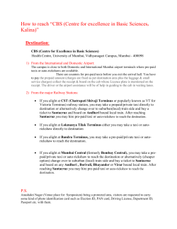
Doxicycline (37 studies from Blume/Mutschler, Bioäquivalenz: Qualitätsbewertung wirkstoffgleicher
ε
Fertigarzneimittel, GOVI-Verlag, Frankfurt am Main/Eschborn, 1989-1996)
χ
ε
Biostatistics:
Biostatistics: Basic concepts & applicable principles for various designs
π Pharma Edge in bioequivalence studies and data analysis | Mumbai,
Mumbai, 29 – 30 January 2011
17 • 49
Sample Size Calculations …or the Myth of Power
Pooling of CV%
Intra-subject
CV from different studies can be
pooled (LA Gould 1995, Patterson and Jones 2006)
In
the parametric model of log-transformed data,
additivity of variances (not of CVs!) apply.
Do not use the arithmetic mean (or the geometric
mean either) of CVs.
Before pooling variances must be weighted
acccording to the studies’ sample size – larger
studies are more influentual than smaller ones.
π
ε
χ
ε
π Pharma Edge
Biostatistics:
Biostatistics: Basic concepts & applicable principles for various designs
in bioequivalence studies and data analysis | Mumbai,
Mumbai, 29 – 30 January 2011
18 • 49
Sample Size Calculations …or the Myth of Power
Pooling of CV%
Intra-subject
CV from different studies
Calculate
the variance from CV
2
σ = ln(CVintra
+ 1)
Calculate the total variance weighted by df
2
σ
∑ W df
Calculate the pooled CV from total variance
σW2 df ∑df
∑
CV = e
−1
2
W
calculate an upper (1–α) % confidence
limit on the pooled CV (recommended α = 0.25)
σW2 df χα2 ,∑df
∑
CL = e
−1
Optionally
π
ε
χ
ε
π Pharma Edge
CV
Biostatistics:
Biostatistics: Basic concepts & applicable principles for various designs
in bioequivalence studies and data analysis | Mumbai,
Mumbai, 29 – 30 January 2011
19 • 49
Sample Size Calculations …or the Myth of Power
Pooling of CV%
Example
1: n1=n2;
CVStudy1 < CVStudy2
studies N
2
24
df (total)
20
α
0.25
σW
CVintra
n
seq.
df (mj)
0.200
0.300
12
12
2
2
10
10
π
ε
χ
ε
π Pharma Edge
1–α
CVpooled CVmean
0.254
0.245
0.291 +14.3%
0.75
χ ²(α ,df)
total
1.2540
15.452
σ ²W
σ ²W × df
CVintra /
pooled
>CLupper
0.3922
0.8618
78.6%
117.9%
no
yes
0.198 0.0392
0.294 0.0862
Biostatistics:
Biostatistics: Basic concepts & applicable principles for various designs
in bioequivalence studies and data analysis | Mumbai,
Mumbai, 29 – 30 January 2011
20 • 49
Sample Size Calculations …or the Myth of Power
Pooling of CV%
Example
2: n1<n2;
CVStudy1 < CVStudy2
studies N
2
36
df (total)
32
α
0.25
σW
CVintra
n
seq.
df (mj)
0.200
0.300
12
24
2
2
10
22
π
ε
χ
ε
π Pharma Edge
1–α
CVpooled CVmean
0.272
0.245
0.301 +10.7%
0.75
χ ²(α ,df)
total
2.2881
26.304
σ ²W
σ ²W × df
CVintra /
pooled
>CLupper
0.3922
1.8959
73.5%
110.2%
no
no
0.198 0.0392
0.294 0.0862
Biostatistics:
Biostatistics: Basic concepts & applicable principles for various designs
in bioequivalence studies and data analysis | Mumbai,
Mumbai, 29 – 30 January 2011
21 • 49
Sample Size Calculations …or the Myth of Power
Pooling of CV%
Example
3: n1>n2;
CVStudy1 < CVStudy2
studies N
2
36
df (total)
32
α
0.25
σW
CVintra
n
seq.
df (mj)
0.200
0.300
24
12
2
2
22
10
π
ε
χ
ε
π Pharma Edge
1–α
CVpooled CVmean
0.235
0.245
0.260 +10.6%
0.75
χ ²(α ,df)
total
1.7246
26.304
σ ²W
σ ²W × df
CVintra /
pooled
>CLupper
0.8629
0.8618
85.0%
127.5%
no
yes
0.198 0.0392
0.294 0.0862
Biostatistics:
Biostatistics: Basic concepts & applicable principles for various designs
in bioequivalence studies and data analysis | Mumbai,
Mumbai, 29 – 30 January 2011
22 • 49
Sample Size Calculations …or the Myth of Power
Pooling of CV%
package PowerTost function CVpooled,
data of last example.
R
require(PowerTOST)
CVs <- ("
PKmetric | CV | n | design | source
AUC
| 0.20 | 24 | 2x2
| study 1
AUC
| 0.30 | 12 | 2x2
| study 2
")
txtcon <- textConnection(CVs)
CVdata <- read.table(txtcon, header=TRUE, sep="|",
strip.white=TRUE, as.is=TRUE)
close(txtcon)
CVsAUC <- subset(CVdata,PKmetric=="AUC")
print(CVpooled(CVsAUC, alpha=0.25), digits=3, verbose=TRUE)
Pooled CV = 0.235 with 32 degrees of freedom
Upper 75% confidence limit of CV = 0.260
π
ε
χ
ε
π Pharma Edge
Biostatistics:
Biostatistics: Basic concepts & applicable principles for various designs
in bioequivalence studies and data analysis | Mumbai,
Mumbai, 29 – 30 January 2011
23 • 49
Sample Size Calculations …or the Myth of Power
Pooling of CV%
Or
you may combine pooling with an estimated
sample size based on uncertain CVs (we will
see later what that means).
R package PowerTost function expsampleN.TOST,
data of last example.
CVs and degrees of freedom must be given as
vectors:
CV = c(0.2,0.3), dfCV = c(22,10)
π
ε
χ
ε
π Pharma Edge
Biostatistics:
Biostatistics: Basic concepts & applicable principles for various designs
in bioequivalence studies and data analysis | Mumbai,
Mumbai, 29 – 30 January 2011
24 • 49
Sample Size Calculations …or the Myth of Power
Pooling of CV%
require(PowerTOST)
expsampleN.TOST(alpha=0.05,
targetpower=0.8,
theta1=0.8, theta2=1.25,
theta0=0.95, CV=c(0.2,0.3),
dfCV=c(22,10), alpha2=0.05,
design="2x2", print=TRUE,
details=TRUE)
++++++++ Equivalence test - TOST ++++++++
Sample size est. with uncertain CV
----------------------------------------Study design: 2x2 crossover
Design characteristics:
df = n-2, design const. = 2, step = 2
log-transformed data (multiplicative model)
alpha = 0.05, target power = 0.8
BE margins
= 0.8 ... 1.25
Null (true) ratio = 0.95
Variability data
CV df
0.2 22
0.3 10
CV(pooled)
= 0.2353158 with 32 df
one-sided upper CL = 0.2995364 (level = 95%)
π
ε
χ
ε
π Pharma Edge
Sample size search
n
exp. power
24
0.766585
26
0.800334
Biostatistics:
Biostatistics: Basic concepts & applicable principles for various designs
in bioequivalence studies and data analysis | Mumbai,
Mumbai, 29 – 30 January 2011
25 • 49
Sample Size Calculations …or the Myth of Power
α- vs. β-Error
α-Error:
Patient’s risk to be treated with a
bioinequivalent formulation.
Although
α is generally set to 0.05, sometimes <0.05
(e.g., NTDIs in Brazil, multiplicity, interim analyses).
β-Error:
Producer’s risk to get no approval for a
bioequivalent formulation.
set in study planning to ≤0.2, where
power = 1 – β = ≥80%.
There is no a posteriori (aka post hoc) power!
Either a study has demonstrated BE or not.
Phoenix’/WinNonlin’s output is statistical nonsense!
Generally
π
ε
χ
ε
π Pharma Edge
Biostatistics:
Biostatistics: Basic concepts & applicable principles for various designs
in bioequivalence studies and data analysis | Mumbai,
Mumbai, 29 – 30 January 2011
26 • 49
Sample Size Calculations …or the Myth of Power
Power Curves
n
24 → 16:
power 0.896→ 0.735
2×2 Cross-over
1
36
24
0.9
16
0.8
0.7
Power
Power to show
BE with 12 – 36
subjects for
CVintra = 20%
12
0.6
0.5
20% CV
0.4
0.3
0.2
µT/µR
1.05 → 1.10:
power 0.903→ 0.700
π
ε
χ
ε
π Pharma Edge
0.1
0
0.8
0.85
0.9
0.95
1
1.05
1.1
1.15
1.2
1.25
µT/µR
Biostatistics:
Biostatistics: Basic concepts & applicable principles for various designs
in bioequivalence studies and data analysis | Mumbai,
Mumbai, 29 – 30 January 2011
27 • 49
Sample Size Calculations …or the Myth of Power
Power vs. Sample Size
It
is not possible to directly calculate the
required sample size.
Power is calculated instead, and the lowest
sample size which fulfills the minimum target
power is used.
Example:
π
ε
χ
ε
π Pharma Edge
α 0.05, target power 80%
(β 0.2), T/R 0.95, CVintra 20% →
minimum sample size 19 (power 81%),
rounded up to the next even number in
a 2×2 study (power 83%).
Biostatistics:
Biostatistics: Basic concepts & applicable principles for various designs
in bioequivalence studies and data analysis | Mumbai,
Mumbai, 29 – 30 January 2011
n
16
17
18
19
20
power
73.54%
76.51%
79.12%
81.43%
83.47%
28 • 49
Sample Size Calculations …or the Myth of Power
Power vs. Sample Size
2×2 cross-over, T/R 0.95, 80%–125%, target power 80%
sample size
power
power for n=12
100%
40
32
24
90%
power
sample size
95%
16
85%
8
π
ε
χ
ε
π Pharma Edge
0
5%
80%
10%
15%
20%
25%
30%
CVintra
Biostatistics:
Biostatistics: Basic concepts & applicable principles for various designs
in bioequivalence studies and data analysis | Mumbai,
Mumbai, 29 – 30 January 2011
29 • 49
Sample Size Calculations …or the Myth of Power
Tools
Sample
Size Tables (Phillips, Diletti, Hauschke,
Chow, Julious, …)
Approximations (Diletti, Chow, Julious, …)
General purpose (SAS, R, S+, StaTable, …)
Specialized Software (nQuery Advisor, PASS,
FARTSSIE, StudySize, …)
Exact method (Owen – implemented in Rpackage PowerTOST)*
* Thanks to Detlew Labes!
π
ε
χ
ε
Biostatistics:
Biostatistics: Basic concepts & applicable principles for various designs
π Pharma Edge in bioequivalence studies and data analysis | Mumbai,
Mumbai, 29 – 30 January 2011
30 • 49
Sample Size Calculations …or the Myth of Power
Background
Reminder:
Sample Size is not directly
obtained; only power
Solution given by DB Owen (1965) as a
difference of two bivariate noncentral
t-distributions
Definite
integrals cannot be solved in closed form
‘Exact’
methods rely on numerical methods (currently
the most advanced is AS 243 of RV Lenth;
implemented in R, FARTSSIE, EFG). nQuery uses an
earlier version (AS 184).
π
ε
χ
ε
π Pharma Edge
Biostatistics:
Biostatistics: Basic concepts & applicable principles for various designs
in bioequivalence studies and data analysis | Mumbai,
Mumbai, 29 – 30 January 2011
31 • 49
Sample Size Calculations …or the Myth of Power
Background
Power
calculations…
‘Brute
force’ methods (also called ‘resampling’ or
‘Monte Carlo’) converge asymptotically to the true
power; need a good random number generator (e.g.,
Mersenne Twister) and may be time-consuming
‘Asymptotic’ methods use large sample
approximations
Approximations
provide algorithms which should
converge to the desired power based on the
t-distribution
π
ε
χ
ε
π Pharma Edge
Biostatistics:
Biostatistics: Basic concepts & applicable principles for various designs
in bioequivalence studies and data analysis | Mumbai,
Mumbai, 29 – 30 January 2011
32 • 49
Sample Size Calculations …or the Myth of Power
Comparison
original values
PowerTOST 0.8-2 (2011)
Patterson & Jones (2006)
Diletti et al. (1991)
nQuery Advisor 7 (2007)
FARTSSIE 1.6 (2008)
Method
exact
noncentr. t
noncentr. t
noncentr. t
noncentr. t
noncentr. t
EFG 2.01 (2009)
brute force
StudySize 2.0.1 (2006)
central t
Hauschke et al. (1992)
approx. t
Chow & Wang (2001)
approx. t
Kieser & Hauschke (1999) approx. t
original values
PowerTOST 0.8-2 (2011)
Patterson & Jones (2006)
Diletti et al. (1991)
nQuery Advisor 7 (2007)
FARTSSIE 1.6 (2008)
π
ε
χ
ε
π Pharma Edge
Method
exact
noncentr. t
noncentr. t
noncentr. t
noncentr. t
noncentr. t
EFG 2.01 (2009)
brute force
StudySize 2.0.1 (2006)
central t
Hauschke et al. (1992)
approx. t
Chow & Wang (2001)
approx. t
Kieser & Hauschke (1999) approx. t
CV%
Algorithm
5 7.5 10 12 12.5 14 15 16 17.5 18 20 22
Owen’s Q 4 6
8
8 10 12 12 14 16 16 20 22
AS 243
4 5
7
8
9 11 12 13 15 16 19 22
Owen’s Q 4 5
7 NA
9 NA 12 NA 15 NA 19 NA
AS 184
4 6
8
8 10 12 12 14 16 16 20 22
AS 243
4 5
7
8
9 11 12 13 15 16 19 22
AS 243
4 5
7
8
9 11 12 13 15 16 19 22
ElMaestro 4 5
7
8
9 11 12 13 15 16 19 22
?
NA 5
7
8
9 11 12 13 15 16 19 22
NA NA
8
8 10 12 12 14 16 16 20 22
NA 6
6
8
8 10 12 12 14 16 18 22
2 NA
6
8 NA 10 12 14 NA 16 20 24
CV%
Algorithm 22.5 24 25 26 27.5 28 30 32 34 36 38 40
Owen’s Q 24 26 28 30 34 34 40 44 50 54 60 66
AS 243
23 26 28 30 33 34 39 44 49 54 60 66
Owen’s Q 23 NA 28 NA 33 NA 39 NA NA NA NA NA
AS 184
24 26 28 30 34 34 40 44 50 54 60 66
AS 243
23 26 28 30 33 34 39 44 49 54 60 66
AS 243
23 26 28 30 33 34 39 44 49 54 60 66
ElMaestro 23 26 28 30 33 34 39 44 49 54 60 66
?
23 26 28 30 33 34 39 44 49 54 60 66
24 26 28 30 34 36 40 46 50 56 64 70
24 26 28 30 34 34 38 44 50 56 62 68
NA 28 30 32 NA 38 42 48 54 60 66 74
Biostatistics:
Biostatistics: Basic concepts & applicable principles for various designs
in bioequivalence studies and data analysis | Mumbai,
Mumbai, 29 – 30 January 2011
33 • 49
Sample Size Calculations …or the Myth of Power
Approximations
Hauschke et al. (1992)
S-C Chow and H Wang (2001)
Patient’s risk α 0.05, Power 80% (Producer’s risk β
0.2), AR [0.80 – 1.25], CV 0.2 (20%), T/R 0.95
1. ∆ = ln(0.8)-ln(T/R) = -0.1719
2. Start with e.g. n=8/sequence
1. df = n 2 – 1 = 8 × 2 - 1 = 14
2. tα,df = 1.7613
3. tβ,df = 0.8681
4. new n = [(tα,df + tβ,df)²(CV/∆)]² =
(1.7613+0.8681)² × (-0.2/0.1719)² = 9.3580
3. Continue with n=9.3580/sequence (N=18.716 → 19)
1. df = 16.716; roundup to the next integer 17
2. tα,df = 1.7396
3. tβ,df = 0.8633
4. new n = [(tα,df + tβ,df)²(CV/∆)]² =
(1.7396+0.8633)² × (-0.2/0.1719)² = 9.1711
4. Continue with n=9.1711/sequence (N=18.3422 → 19)
1. df = 17.342; roundup to the next integer 18
2. tα,df = 1.7341
3. tβ,df = 0.8620
4. new n = [(tα,df + tβ,df)²(CV/∆)]² =
(1.7341+0.8620)² × (-0.2/0.1719)² = 9.1233
5. Convergence reached (N=18.2466 → 19):
Patient’s risk α 0.05, Power 80% (Producer’s risk β
0.2), AR [0.80 – 1.25], CV 0.2 (20%), T/R 0.95
1. ∆ = ln(T/R) – ln(1.25) = 0.1719
2. Start with e.g. n=8/sequence
1. dfα = roundup(2n-2)2-2 = (2×8-2)×2-2 = 26
2. dfβ = roundup(4n-2) = 4×8-2 = 30
3. tα,df = 1.7056
4. tβ/2,df = 0.8538
5. new n = β²[(tα,df + tβ/2,df)²/∆² =
0.2² × (1.7056+0.8538)² / 0.1719² = 8.8723
3. Continue with n=8.8723/sequence (N=17.7446 → 18)
1. dfα = roundup(2n-2)2-2=(2×8.8723-2)×2-2 = 30
2. dfβ = roundup(4n-2) = 4×8.8723-2 = 34
3. tα,df = 1.6973
4. tβ/2,df = 0.8523
5. new n = β²[(tα,df + tβ/2,df)²/∆² =
0.2² × (1.6973+0.8538)² / 0.1719² = 8.8045
4. Convergence reached (N=17.6090 → 18):
Use 9 subjects/sequence (18 total)
sample size
18
π
Use 10 subjects/sequence (20 total)
ε
power %
79.124
χ
ε
Biostatistics:
Biostatistics: Basic concepts & applicable principles for various designs
π Pharma Edge in bioequivalence studies and data analysis | Mumbai,
Mumbai, 29 – 30 January 2011
19
20
81.428
83.468
34 • 49
Sample Size Calculations …or the Myth of Power
Approximations obsolete
Exact
sample size tables still useful in
checking the plausibility of software’s results
Approximations
based on
noncentral t (FARTSSIE17)
http://individual.utoronto.ca/ddubins/FARTSSIE17.xls
or
/ S+ →
Exact method (Owen) in
R-package PowerTOST
http://cran.r-project.org/web/packages/PowerTOST/
π
ε
χ
ε
π Pharma Edge
require(PowerTOST)
sampleN.TOST(alpha = 0.05,
targetpower = 0.80, logscale = TRUE,
theta1 = 0.80, diff = 0.95, CV = 0.30,
design = "2x2", exact = TRUE)
alpha
<- 0.05
# alpha
CV
<- 0.30
# intra-subject CV
theta1 <- 0.80
# lower acceptance limit
theta2 <- 1/theta1 # upper acceptance limit
ratio
<- 0.95
# expected ratio T/R
PwrNeed <- 0.80
# minimum power
Limit
<- 1000
# Upper Limit for Search
n
<- 4
# start value of sample size search
s
<- sqrt(2)*sqrt(log(CV^2+1))
repeat{
t
<- qt(1-alpha,n-2)
nc1
<- sqrt(n)*(log(ratio)-log(theta1))/s
nc2
<- sqrt(n)*(log(ratio)-log(theta2))/s
prob1 <- pt(+t,n-2,nc1); prob2 <- pt(-t,n-2,nc2)
power <- prob2-prob1
n
<- n+2
# increment sample size
if(power >= PwrNeed | (n-2) >= Limit) break }
Total
<- n-2
if(Total == Limit){
cat("Search stopped at Limit",Limit,
" obtained Power",power*100,"%\n")
} else
cat("Sample Size",Total,"(Power",power*100,"%)\n")
Biostatistics:
Biostatistics: Basic concepts & applicable principles for various designs
in bioequivalence studies and data analysis | Mumbai,
Mumbai, 29 – 30 January 2011
35 • 49
Sample Size Calculations …or the Myth of Power
Sensitivity Analysis
ICH
E9 (1998)
Section
3.5 Sample Size, paragraph 3
The method by which the sample size is calculated
should be given in the protocol […]. The basis of
these estimates should also be given.
It is important to investigate the sensitivity of the
sample size estimate to a variety of deviations from
these assumptions and this may be facilitated by
providing a range of sample sizes appropriate for a
reasonable range of deviations from assumptions.
In confirmatory trials, assumptions should normally
be based on published data or on the results of
earlier trials.
π
ε
χ
ε
π Pharma Edge
Biostatistics:
Biostatistics: Basic concepts & applicable principles for various designs
in bioequivalence studies and data analysis | Mumbai,
Mumbai, 29 – 30 January 2011
36 • 49
Sample Size Calculations …or the Myth of Power
Sensitivity Analysis
Example
2
+ 1); ln(0.22 + 1) = 0.198042
nQuery Advisor: σ w = ln(CVintra
20% CV:
n=26
π
ε
χ
ε
π Pharma Edge
25% CV:
power 90% → 78%
20% CV, 4 drop outs:
power 90% → 87%
20% CV, PE 90%:
power 90% → 67%
25% CV, 4 drop outs:
power 90% → 70%
Biostatistics:
Biostatistics: Basic concepts & applicable principles for various designs
in bioequivalence studies and data analysis | Mumbai,
Mumbai, 29 – 30 January 2011
37 • 49
Sample Size Calculations …or the Myth of Power
Sensitivity Analysis
Example
PowerTOST, function sampleN.TOST
require(PowerTost)
sampleN.TOST(alpha = 0.05, targetpower = 0.9, logscale = TRUE,
theta1 = 0.8, theta2 = 1.25, theta0 = 0.95, CV = 0.2,
design = "2x2", exact = TRUE, print = TRUE)
π
ε
χ
ε
π Pharma Edge
+++++++++++ Equivalence test - TOST +++++++++++
Sample size estimation
----------------------------------------------Study design: 2x2 crossover
log-transformed data (multiplicative model)
alpha = 0.05, target power = 0.9
BE margins
= 0.8 ... 1.25
Null (true) ratio = 0.95, CV = 0.2
Sample size
n
power
26
0.917633
Biostatistics:
Biostatistics: Basic concepts & applicable principles for various designs
in bioequivalence studies and data analysis | Mumbai,
Mumbai, 29 – 30 January 2011
38 • 49
Sample Size Calculations …or the Myth of Power
Sensitivity Analysis
To
calculate Power for a given sample size,
use function power.TOST
π
ε
χ
ε
π Pharma Edge
require(PowerTost)
power.TOST(alpha=0.05, logscale=TRUE, theta1=0.8, theta2=1.25,
theta0=0.95, CV=0.25, n=26, design="2x2", exact=TRUE)
[1] 0.7760553
power.TOST(alpha=0.05, logscale=TRUE, theta1=0.8, theta2=1.25,
theta0=0.95, CV=0.20, n=22, design="2x2", exact=TRUE)
[1] 0.8688866
power.TOST(alpha=0.05, logscale=TRUE, theta1=0.8, theta2=1.25,
theta0=0.95, CV=0.25, n=22, design="2x2", exact=TRUE)
[1] 0.6953401
power.TOST(alpha=0.05, logscale=TRUE, theta1=0.8, theta2=1.25,
theta0=0.90, CV=0.20, n=26, design="2x2", exact=TRUE)
[1] 0.6694514
power.TOST(alpha=0.05, logscale=TRUE, theta1=0.8, theta2=1.25,
theta0=0.90, CV=0.25, n=22, design="2x2", exact=TRUE)
[1] 0.4509864
Biostatistics:
Biostatistics: Basic concepts & applicable principles for various designs
in bioequivalence studies and data analysis | Mumbai,
Mumbai, 29 – 30 January 2011
39 • 49
Sample Size Calculations …or the Myth of Power
Sensitivity Analysis
Must
be done before the study (a priori)
The Myth of retrospective (a posteriori)
Power…
High
values do not further support the claim of
already demonstrated bioequivalence.
Low values do not invalidate a bioequivalent
formulation.
Further reader:
π
ε
χ
ε
π Pharma Edge
RV Lenth (2000)
JM Hoenig and DM Heisey (2001)
P Bacchetti (2010)
Biostatistics:
Biostatistics: Basic concepts & applicable principles for various designs
in bioequivalence studies and data analysis | Mumbai,
Mumbai, 29 – 30 January 2011
40 • 49
Sample Size Calculations …or the Myth of Power
Data from Pilot Studies
Estimated
CVs have a high degree of uncertainty (in the pivotal study it is more likely that
you will be able to reproduce the PE, than the
CV)
The
π
ε
χ
ε
π Pharma Edge
smaller the size of the pilot,
the more uncertain the outcome.
The more formulations you have
tested, lesser degrees of freedom
will result in worse estimates.
Remember: CV is an estimate –
not carved in stone!
Biostatistics:
Biostatistics: Basic concepts & applicable principles for various designs
in bioequivalence studies and data analysis | Mumbai,
Mumbai, 29 – 30 January 2011
41 • 49
Sample Size Calculations …or the Myth of Power
Pilot Studies: Sample Size
Small
pilot studies (sample size <12)
Are
useful in checking the sampling schedule and
the appropriateness of the analytical method, but
are not suitable for the purpose of sample size
planning!
Sample sizes (T/R 0.95,
CV
ratio
CV%
fixed uncertain uncert./fixed
power ≥80%) based on
20
20
24
1.200
a n=10 pilot study
π
ε
χ
ε
π Pharma Edge
require(PowerTOST)
expsampleN.TOST(alpha=0.05,
targetpower=0.80, theta1=0.80,
theta2=1.25, theta0=0.95, CV=0.40,
dfCV=24-2, alpha2=0.05, design="2x2")
25
28
36
1.286
30
40
52
1.300
35
52
68
1.308
40
66
86
1.303
Biostatistics:
Biostatistics: Basic concepts & applicable principles for various designs
in bioequivalence studies and data analysis | Mumbai,
Mumbai, 29 – 30 January 2011
If pilot n=24:
n=72, ratio 1.091
42 • 49
Sample Size Calculations …or the Myth of Power
Pilot Studies: Sample Size
Moderate
sized pilot studies (sample size
~12–24) lead to more consistent results
(both CV and PE).
If
π
ε
χ
ε
π Pharma Edge
you stated a procedure in your protocol, even
BE may be claimed in the pilot study, and no
further study will be necessary (US-FDA).
If you have some previous hints of high intrasubject variability (>30%), a pilot study size of
at least 24 subjects is reasonable.
A Sequential Design may also avoid an
unnecessarily large pivotal study.
Biostatistics:
Biostatistics: Basic concepts & applicable principles for various designs
in bioequivalence studies and data analysis | Mumbai,
Mumbai, 29 – 30 January 2011
43 • 49
Sample Size Calculations …or the Myth of Power
Pilot Studies: Sample Size
Do
not use the pilot study’s CV, but calculate
an upper confidence interval!
Gould
(1995) recommends a 75% CI (i.e., a
producer’s risk of 25%).
Apply Bayesian Methods (Julious and Owen 2006,
Julious 2010) implemented in R’s
PowerTOST/expsampleN.TOST.
Unless you are under time pressure, a Two-Stage
Sequential Design will help in dealing with the
uncertain estimate from the pilot study.
π
ε
χ
ε
π Pharma Edge
Biostatistics:
Biostatistics: Basic concepts & applicable principles for various designs
in bioequivalence studies and data analysis | Mumbai,
Mumbai, 29 – 30 January 2011
44 • 49
Sample Size Calculations …or the Myth of Power
Sample Size Calculations
…or the Myth of Power
Helmut Schütz
BEBAC
π
ε
χ
ε
π Pharma Edge
Consultancy Services for
Bioequivalence and Bioavailability Studies
1070 Vienna, Austria
[email protected]
Biostatistics:
Biostatistics: Basic concepts & applicable principles for various designs
in bioequivalence studies and data analysis | Mumbai,
Mumbai, 29 – 30 January 2011
45 • 49
Sample Size Calculations …or the Myth of Power
To bear in Remembrance...
Power. That which statisticians are always calculating
but never have.
Power: That which is wielded by the priesthood of
clinical trials, the statisticians, and a stick which they
use to beta their colleagues.
Power Calculation – A guess masquerading as mathematics.
Stephen Senn
You should treat as many patients as possible with the
new drugs while they still have the power to heal.
Armand Trousseau
π
ε
χ
ε
π Pharma Edge
Biostatistics:
Biostatistics: Basic concepts & applicable principles for various designs
in bioequivalence studies and data analysis | Mumbai,
Mumbai, 29 – 30 January 2011
46 • 49
Sample Size Calculations …or the Myth of Power
The Myth of Power
There is simple intuition behind
results like these: If my car made
it to the top of the hill, then it is
powerful enough to climb that hill;
if it didn’t, then it obviously isn’t
powerful enough. Retrospective
power is an obvious answer to a
rather uninteresting question. A
more meaningful question is to
ask whether the car is powerful
enough to climb a particular hill
never climbed before; or whether
a different car can climb that new
hill. Such questions are prospective, not retrospective.
π
ε
χ
ε
π Pharma Edge
The fact that retrospective
power adds no new information is harmless in its
own right. However, in
typical practice, it is used
to exaggerate the validity of a significant result (“not only is it significant,
but the test is really powerful!”), or to
make excuses for a nonsignificant
one (“well, P is .38, but that’s only
because the test isn’t very powerful”).
The latter case is like blaming the
messenger.
RV Lenth
Two Sample-Size Practices that I don't recommend
http://www.math.uiowa.edu/~rlenth/Power/2badHabits.pdf
Biostatistics:
Biostatistics: Basic concepts & applicable principles for various designs
in bioequivalence studies and data analysis | Mumbai,
Mumbai, 29 – 30 January 2011
47 • 49
Sample Size Calculations …or the Myth of Power
References
Collection
of links to global documents
http://bebac.at/Guidelines.htm
ICH
E9: Statistical Principles for Clinical Trials (1998)
EMA-CPMP/CHMP/EWP
Points to Consider on Multiplicity Issues in Clinical
Trials (2002)
BA/BE for HVDs/HVDPs: Concept Paper (2006)
http://bebac.at/downloads/14723106en.pdf
Questions & Answers on the BA and BE Guideline
(2006) http://bebac.at/downloads/4032606en.pdf
Draft Guideline on the Investigation of BE (2008)
Guideline on the Investigation of BE (2010)
Questions & Answers: Positions on specific questions
addressed to the EWP therapeutic subgroup on
Pharmacokinetics (2010)
US-FDA
Center for Drug Evaluation and Research (CDER)
Statistical Approaches Establishing
Bioequivalence (2001)
Bioequivalence Recommendations for Specific
Products (2007)
π
ε
χ
ε
π Pharma Edge
Midha KK, Ormsby ED, Hubbard JW, McKay G, Hawes EM,
Gavalas L, and IJ McGilveray
Logarithmic Transformation in Bioequivalence: Application
with Two Formulations of Perphenazine
J Pharm Sci 82/2, 138-144 (1993)
Hauschke D, Steinijans VW, and E Diletti
Presentation of the intrasubject coefficient of variation for
sample size planning in bioequivalence studies
Int J Clin Pharmacol Ther 32/7, 376-378 (1994)
Diletti E, Hauschke D, and VW Steinijans
Sample size determination for bioequivalence assessment by
means of confidence intervals
Int J Clin Pharm Ther Toxicol 29/1, 1-8 (1991)
Hauschke D, Steinijans VW, Diletti E, and M Burke
Sample Size Determination for Bioequivalence Assessment
Using a Multiplicative Model
J Pharmacokin Biopharm 20/5, 557-561 (1992)
S-C Chow and H Wang
On Sample Size Calculation in Bioequivalence Trials
J Pharmacokin Pharmacodyn 28/2, 155-169 (2001)
Errata: J Pharmacokin Pharmacodyn 29/2, 101-102 (2002)
DB Owen
A special case of a bivariate non-central t-distribution
Biometrika 52, 3/4, 437-446 (1965)
Biostatistics:
Biostatistics: Basic concepts & applicable principles for various designs
in bioequivalence studies and data analysis | Mumbai,
Mumbai, 29 – 30 January 2011
48 • 49
Sample Size Calculations …or the Myth of Power
References
LA Gould
Group Sequential Extension of a Standard Bioequivalence
Testing Procedure
J Pharmacokin Biopharm 23/1, 57–86 (1995)
DOI: 10.1007/BF02353786
Tóthfalusi L, Endrenyi L, and A Garcia Arieta
Evaluation of Bioequivalence for Highly Variable Drugs
with Scaled Average Bioequivalence
Clin Pharmacokinet 48/11, 725-743 (2009)
RV Lenth
Two Sample-Size Practices that I don’t recommend
Joint Statistical Meetings, Indianapolis (2000)
http://www.math.uiowa.edu/~rlenth/Power/2badHabits.pdf
Hoenig JM and DM Heisey
The Abuse of Power: The Pervasive Fallacy of Power
Calculations for Data Analysis
The American Statistician 55/1, 19–24 (2001)
http://www.vims.edu/people/hoenig_jm/pubs/hoenig2.pdf
P Bacchetti
Current sample size conventions: Flaws, harms, and
alternatives
BMC Medicine 8:17 (2010)
http://www.biomedcentral.com/content/pdf/1741-7015-817.pdf
π
ε
χ
ε
π Pharma Edge
Jones B and MG Kenward
Design and Analysis of Cross-Over Trials
Chapman & Hall/CRC, Boca Raton (2nd Edition 2000)
Patterson S and B Jones
Determining Sample Size, in:
Bioequivalence and Statistics in Clinical Pharmacology
Chapman & Hall/CRC, Boca Raton (2006)
SA Julious
Tutorial in Biostatistics. Sample sizes for clinical trials with
Normal data
Statistics in Medicine 23/12, 1921-1986 (2004)
Julious SA and RJ Owen
Sample size calculations for clinical studies allowing for
uncertainty about the variance
Pharmaceutical Statistics 5/1, 29-37 (2006)
SA Julious
Sample Sizes for Clinical Trials
Chapman & Hall/CRC, Boca Raton (2010)
D Labes
Package ‘PowerTOST’
Version 0.8-2 (2011-01-10)
http://cran.rproject.org/web/packages/PowerTOST/PowerTOST.pdf
Biostatistics:
Biostatistics: Basic concepts & applicable principles for various designs
in bioequivalence studies and data analysis | Mumbai,
Mumbai, 29 – 30 January 2011
49 • 49