1. No category

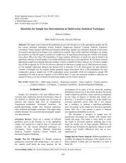
Survey Research Methods (2009)
Vol.3, No.1, pp. 45-58
ISSN 1864-3361
http://www.surveymethods.org
c European Survey Research Association
A Monte Carlo sample size study: How many countries are needed for
accurate multilevel SEM?
Bart Meuleman and Jaak Billiet
University of Leuven
Recently, there has been growing scientific interest for cross-national survey research. Various
scholars have used multilevel techniques to link individual characteristics to aspects of the national context. At first sight, multilevel SEM seems to be a promising tool for this purpose, as
it integrates multilevel modeling within a latent variable framework. However, due to the fact
that the number of countries in most international surveys does not exceed 30, the application
of multilevel SEM in cross-national research is problematic.
Taking European Social Survey (ESS) data as a point of departure, this paper uses Monte Carlo
studies to assess the estimation accuracy of multilevel SEM with small group sample sizes. The
results indicate that a group sample size of 20 – a situation common in cross-national research
– does not guarantee accurate estimation at all. Unacceptable amounts of parameter and standard error bias are present for the between-level estimates. Unless the standardized effect is
very large (0.75), statistical power for detecting a significant between-level structural effect is
seriously lacking. Required group sample sizes depend strongly on the specific interests of
the researcher, the expected effect sizes and the complexity of the model. If the between-level
model is relatively simple and one is merely interested in the between-level factor structure,
a group sample size of 40 could be sufficient. To detect large (>0.50) structural effects at the
between level, at least 60 groups are required. To have an acceptable probability of detecting
smaller effects, more than 100 groups are needed. These guidelines are shown to be quite
robust for varying cluster sizes and intra-class correlations (ICCs).
Keywords: multilevel SEM, sample size, Monte Carlo, cross-national research, European Social Survey
1 Introduction
Recently, scientific interest for cross-national survey research is on the rise. Without a doubt, this tendency is at
least partly a result of the increasing availability of data from
international surveys, such as the International Social Survey
Program, the Europe and World Value Studies or the European Social Survey. These rich data sources offer attractive
perspectives for social scientists. Various scholars have used
cross-national survey data to investigate the relation between
elements of the national context and individual characteristics (for some examples of contextual research into out-group
attitudes, see: Quillian 1995; Lubbers et al. 2002; Scheepers
et al. 2002; Coenders and Scheepers 2003; Kunovich 2004;
Semyonov et al. 2006; Sides and Citrin 2007). From a substantive point of view, this approach is highly relevant. After
all, the idea that individuals are influenced by the broader
context they are situated in is a cornerstone of social science.
Also from a modeler’s perspective, the relation between
national- and individual-level variables raises some interesting questions. It has become quite popular to use multilevel techniques to study the relation between context and
individual variables (Mason et al. 1983-1984). At first
sight, this preference is far from illogical, since these crossnational data exhibit a hierarchical structure: Citizens are
nested within countries. In the vast majority of the cases,
hierarchical linear models (Raudenbush and Bryk 2002) or
random coefficient models (Kreft and de Leeuw 1998) are
employed for the study of context effects (Quillian 1995; Coenders 2001; Lubbers et al. 2002; Coenders and Scheepers
2003; Kunovich 2004; Semyonov et al. 2006). However,
this is not the only possible multilevel approach. More recent
developments in the domain of covariance structure modeling have made it relatively easy to estimate multilevel structural equation models (SEM) (Muth´en 1994; Li et al. 1998;
Hox 2002). As Rabe-Hesketh et al. (2004:167) point out,
“multilevel structural equation modeling is required when
the units of observation form a hierarchy of nested clusters
and some variables of interest cannot be measured directly
but are measured by a set of items or fallible instruments.”
The integration of latent variable modeling within a multilevel framework makes multilevel SEM particularly promising for cross-national attitude research (for an application,
see: Cheung and Au 2005).
Contact information: Bart Meuleman, Centre for Sociological
Research (CeSO) - KU Leuven, Parkstraat 45 box 3601, 3000 Leuven, Belgium, e-mail: [email protected]
Despite the desirable characteristics of multilevel SEM,
its application in the field of cross-national research is far
from straightforward. Due to various methodological issues – such as the cross-cultural comparability of scores
(Steenkamp and Baumgartner 1998; Vandenberg and Lance
45
46
BART MEULEMAN AND JAAK BILLIET
2000) and the absence of random sampling at the country
level – the use of multilevel models in cross-national research
is problematic. Another challenge is that, due to budgetary
and organizational limitations, the number of participating
countries is limited to 20 or 30 for most international surveys (Goldthorpe 1997). The scarce available research into
sufficient sample sizes for multilevel SEM suggests that this
group sample size is too small to guarantee accurate estimation (Hox 1993; Hox and Maas 2001). Based on simulation
studies, Hox and Maas (2001:171) warn against using multilevel SEM when the group sample size is smaller than 100.
However, it is not sure to what extent the results of the Hox
and Maas (2001) study can be extrapolated to the particular situation of cross-national research. First, cross-national
research generally contains a large number of respondents
per country (>1000). These cluster sizes are substantially
larger than the cluster sizes specified in the simulations by
Hox and Maas (2001). Second, the Hox and Maas (2001)
study focused on a two-level measurement model. Crossnational researchers, on the other hand, are often also interested in the structural model, and more specifically in the effects of national context variables on individual characteristics. Third, Hox and Maas (2001) set up their study to gauge
Muth´en’s (1989; 1994) limited information maximum likelihood (LIML) approach, which treats unbalanced groups as if
they were balanced and, therefore, only gives an approximate
solution. However, in more recent versions of the software
package Mplus, the more exact full information maximum
likelihood (FIML) estimation has become available (for continuous data at least) and researchers are no longer compelled
to use the LIML approach.
For the above-mentioned reasons, we are convinced that
it is desirable to study required sample sizes at the group level
for applying multilevel SEM in cross-national research. In
this paper, we present the results of Monte Carlo simulation
studies that were performed with this specific purpose. We
start by introducing Muth´en’s (1994) approach to multilevel
SEM. Second, a simple application of multilevel SEM in the
domain of cross-national attitude research is presented. The
results of this application serve as a starting point for a first
series of simulations, in which we assess the estimation accuracy of models with various group sample sizes. Finally, the
robustness of the findings for changes with respect to other
factors – namely, cluster sizes, intra-class correlations (ICCs)
and model complexity – is studied in the last paragraph.
2 Multilevel SEM: Muth´en’s
(1994) approach
Like other multilevel models, multilevel SEM assumes
random sampling at both individual and group levels. The
total population of N individuals can be subdivided into G
groups. From a covariance structure point of view, the hierarchical nature of the data is incorporated by decomposing
the total covariance matrix orthogonally into (1) a component
that represents the variation between groups (the betweengroup covariance matrix) and (2) a component that describes
variation within the groups (the within-group covariance matrix).
ΣT = ΣB + ΣW
(1)
Multilevel SEM essentially leads to estimating covariance structure models for between-structure ΣB (the so-called
between-model) and within-structure ΣW (the within-model).
Muth´en (1994) developed a ML-based procedure to estimate
the between- and the within-model (see also Hox 1993; Hox
2002; Li et al. 1998; Hox and Maas 2001; Cheung and Au
2005). The starting point of this procedure is the orthogonal
decomposition of the observed score vectors into an individual and a group component.
yT = yB + yW
(2)
Let y ji refer to the vector of observed scores for individual i in group j. Group component yB then equals the group
mean (¯yg ), while individual component yW refers to the individual deviation from this mean (ygi − y¯ g ). Based on these
components, a between-group sample covariance matrix S B
and a pooled within-group covariance matrix S PW can be calculated.
PG
yg − y¯ )(¯yg − y¯ )0
g=1 (¯
SB =
(3)
(G − 1)
PG PNg
¯ g )(ygi − y¯ g )0
g=1 i=1 (ygi − y
S PW =
(4)
(N − G)
The pooled within S PW can be shown to be an unbiased
and consistent estimator of ΣW (Muth´en 1989).
S PW = Σˆ W
(5)
As a consequence, a within-model can be constructed
and tested for S PW analogously as in conventional SEM.
For the between-model, the situation is less clear-cut,
since sample matrix S B cannot be simply used as an estimator of population matrix ΣB . Instead, Muth´en (1989) has
shown that in the balanced case (i.e. if all clusters are of equal
size n), S B is a consistent and unbiased estimator of a linear
combination of the within and between matrices.
S B = Σˆ W + cΣˆ B
(6)
In expression (6), c equals the common cluster size n.
Thus, S B is reproduced by a combination of two models,
namely, the within-group model that was estimated for S PW
and c times the between-model.
When groups are unbalanced, the situation becomes
more complicated. For each set of groups with cluster size
equals to cd , sample matrix S B estimates a different combination of population matrices ΣB and ΣW (Hox and Maas
2001).
S B = Σˆ W + cd Σˆ B
(7)
Software packages such as Mplus 4 (Muth´en and
Muth´en 1998-2006) or LISREL 8.80 (J¨oreskog and S¨orb¨om
1996) allow estimation of multilevel structural equation
A MONTE CARLO SAMPLE SIZE STUDY: HOW MANY COUNTRIES ARE NEEDED FOR ACCURATE MULTILEVEL SEM?
models without having to calculate separate pooled withinand between-group matrices or having to take care of the
technical particularities specified above.
3 Starting point: A multilevel
SEM application to
cross-national attitude research
Before proceeding to the proper simulation studies, we
present a simple application of multilevel SEM in the domain
of cross-national attitude research. This model will serve as
a starting point for the simulation study, in the sense that estimated parameter values will be used as population values
in the Monte Carlo studies (Muth´en and Muth´en 2002).
The main substantive research question is whether individual attitudes towards immigration are influenced by the
size of foreign population in the country. According to realistic group conflict theory (Blalock 1967; Olzak 1992), the
presence of minority groups leads to so-called ethnic competition for scarce goods – such as affordable housing and
well-paid jobs – and results in negative attitudes toward immigration among the native population. For this reason, negative out-group attitudes are expected to be more widespread
in countries with a sizeable minority populations (Quillian
1995; Semyonov et al. 2006). Apart from this national-level
variable, we also include the education level of the respondent as an explanatory variable in the model. A higher educational level is expected to coincide with more positive attitudes towards immigration (Coenders and Scheepers 2003;
Hainmueller and Hiscox 2007).
Data from the first round (2002-2003) of the European
Social Survey are used to test these hypotheses. A total of
39,869 respondents from 21 European countries participated
in this large-scale cross-national survey.1 Here, we operationalize the attitude toward immigration as a latent variable
(‘immig’) measured by means of four items. These items inquire whether respondents prefer their country to allow many
or few immigrants of certain groups (see Table 1 for exact
question wordings). The ICCs of the items range between
0.057 and 0.103. Thus, roughly between 5 and 10% of the total variation in attitudes toward immigration can be attributed
to the national level. This amount of variance at the national
level is perhaps not overwhelming, but is nevertheless too
large to be ignored in analysis. It indicates that the national
context does play a role in the formation of attitudes toward
immigration, although it may only be a minor one. Before
the multilevel SEM model was estimated, we tested if the
immig scale was measured in an equivalent way over countries. By means of multi-group confirmatory factor analysis, partial scalar equivalence of the scale was evidenced (for
more details, see: Meuleman and Billiet 2005). Concretely
this means that, apart from a limited number of exceptions,2
the factor loadings and the intercepts of the measurement
model where found to be invariant over the countries in the
study. This partial equivalence is a prerequisite for making
meaningful comparisons of latent variable scores over cultural groups (Byrne et al. 1989; Steenkamp and Baumgartner
1998).
47
The size of the foreign population is indicated by the percentage of the resident population born outside the country
as reported by the OECD (OECD 2006). Educational level
is operationalized by a variable that ranges from 0 (primary
education not completed) to 6 (second stage of university education).
Figure 1 gives a graphical representation of the estimated
model. At the within level, the four observed indicators load
on one latent factor, that is, ‘immig w’. This latent factor
represents the within-country component of the attitude toward immigration, i.e., corrected for the country-mean. We
estimate the effect of individual-level variable education on
this latent factor. Also at the within level, an error correlation was specified between items d6 and d8. This error
correlation is theoretically justified, since both items have
some content in common that is not accounted for by the latent factor: They refer to immigration from richer countries
specifically. Apart from the error correlation, the same factor
structure is present at the between level (this does not have
to be necessarily so, see Hox 2002). The latent variable at
the between level (‘immig b’) is measured by the betweenlevel components of the indicators (these components would
be called random intercepts in hierarchical linear modeling).
A path is estimated between the national level variable ‘foreign population’ and ‘immig b’. This parameter is the main
parameter of interest in this model, and will be referred to as
the between-level structural effect.
The model was estimated with Mplus 4.0 (Muth´en and
Muth´en 1998-2006).3 The relevant parameter estimates are
summarized in Table 2. All entries in this table are completely standardized parameters. At both levels, the measurement models were identified by constraining the variances
of the latent factor to 1. The chi-square value of the model
equals 309.9. With 13 degrees of freedom, this value has a
p-value smaller than .001. However, the chi-square test is
known to be very sensitive for large sample sizes and deviations from the normality assumptions. Since our sample
is very large (36,978) and the items are heavily skewed, we
1
These countries are: Austria, Belgium, Czech Republic, Denmark, Finland, France, Germany, Greece, Hungary, Italy, Ireland,
Luxemburg, the Netherlands, Norway, Poland, Portugal, Slovenia,
Spain, Switzerland, Sweden, and the United Kingdom. Also, Israel
participated in ESS round 1, but we decided to omit Israel from the
analysis for theoretical reasons. The Israeli case is not comparable
to most European countries because of the specificity of the immigration history and ethnic relations within the country.
2
Concretely, three equivalence constraints had to be relaxed: the
factor loading of the first item for Hungary, and the intercept of
this same item for Hungary and Denmark. This means that three
items were measured in an equivalent way, what is sufficient to
allow meaningful cross-cultural comparisons (Byrne et al. 1989;
Steenkamp and Baumgartner 1998).
3
Robust maximum likelihood estimation (MLR) - the default estimator for two-level models in Mplus (Muth´en and Muth´en 19982006) - was used. Although the attitude indicators are orderedcategorical variables, they are treated as if they were continuous.
For multilevel SEM with ordered-categorical indicators, numerical
integration is used, which is computationally extremely heavy given
the large sample size.
48
BART MEULEMAN AND JAAK BILLIET
Table 1: Formulation of the items on preferred immigration policy
Item
Formulation
Answer scale
To what extent do you think [country] should allow. . .
. . . people of a different race or ethnic group as most [country] people to come and live here?
. . . people from the richer countries in Europe to come and live here?
. . . people from the poorer countries in Europe to come and live here?
. . . people from the richer countries outside Europe to come and live here?
d5
d6
d7
d8
3 Sufficient group sample sizes
for multilevel SEM
immig_b
foreign pop.
allow none = 1
allow a few = 2
allow some = 3
allow many = 4
3.1 Specifications of the simulation model
d5_b
d6_b
d7_b
d8_b
d5
d6
d7
d8
between model
within model
education
Figure 1.
policy
immig_w
A multi-level SEM for attitudes toward immigration
prefer to use alternative indices to evaluate overall model fit.
The RMSEA (0.025) falls well below the common boundary of 0.05 (Browne and Cudeck 1992); CFI and TLI are
substantially larger than 0.95 (Hu and Bentler 1999). This
leads to the conclusion that the overall fit of the model is
acceptable. The factor loadings are high (especially for the
between-model), which means that the indicators measure
the latent concepts adequately.
Conforming to our expectations, education has a positive significant effect on attitudes toward immigration at the
within level. At the between level, the percentage of foreign population has no significant impact on attitudes toward
immigration, which clearly contradicts hypotheses derived
from realistic group conflict theory. After all, this theory
predicts anti-immigration attitudes to be more widespread in
countries with sizeable ethnic minorities, because the latter
condition would set of a process of ethnic competition between majority and minority groups (Blalock 1967; Quillian
1995; Olzak 1992).
However, because our group sample size (21 countries)
is on the small side, it is uncertain whether the parameters on
which these conclusions are based are estimated accurately.
To gain more insight in the consequences of small group
sample sizes in cross-national research and required group
sample size for obtaining accurate parameter estimates in
multilevel SEM, we decided to perform a Monte Carlo simulation study. Data generation and analysis was performed
by means of the Mplus Monte Carlo procedure (Muth´en and
Muth´en 2002). To approximate a realistic cross-national setting as much as possible, the application presented above is
used as a reference point for specifying the simulation model.
After all, numerous factors such as the strength of the relations, the model complexity, and the ICCs could influence
the estimation accuracy (Muth´en and Muth´en 2002).
As in the application, the simulation model contains a
within- and a between-level factor measured by four indicators. At each level, one structural path is estimated from an
independent variable to the latent factor. The simulated data
sets were generated as random samples from a hypothesized
population with the following specifications:4
• The observed variables (indicators y1 − y4, individual level variable x and between-level variable b) are
drawn from a multivariate normal distribution.
• The ICC of the four items y1 − y4 is 0.08.5
• The within-level standardized factor loadings equal
0.90, 0.90, 0.75, and 0.70.
• The between-level standardized factor loadings are
0.90, 0.90, 0.95, and 0.95.
• Within-level independent variable x has a standardized
effect of 0.25 on the within-level factor.
• Between-level independent variable b has an effect on
the between-level factor.
Our main interest is the relation between the independent
variable and the latent factor on the between level. Since
estimation accuracy can be influenced by the effect size,
we decided to specify various effect size conditions for the
4
The within- and between-level population covariance matrices
and mean vectors for this baseline model have been added in the
appendix.
5
The ICC value can be chosen by manipulating the ratio of the
between-level variance and the total variance of the indicators. In
these models, the within-level and between-level variances of the
indicators were specified to equal 1 and 0.087 respectively, which
results in an ICC of 0.08.
49
A MONTE CARLO SAMPLE SIZE STUDY: HOW MANY COUNTRIES ARE NEEDED FOR ACCURATE MULTILEVEL SEM?
Table 2: Completely standardized parameter estimates for the multilevel SEM (21 countries; N = 36,978)
Measurement model parameters
Factor loadings
d5
d6
d7
d8
Corr(d6,d8)
Within model
Between model
parameter
t-value
parameter
t-value
0.89
0.70
0.89
0.74
0.31
52.48
40.91
46.49
42.96
17.45
0.99
0.93
0.99
0.91
5.21
5.94
5.36
5.54
0.24
16.62
Structural model parameters
Effect education
Effect foreign pop.
Fit indices
0.09
χ2 = 309.9 df = 13 RMSEA = 0.025 CFI = 0.984 TLI = 0.971
between-level structural effect. Based on Cohen’s (Cohen
1992) categorization scheme for effect sizes, a distinction is
made between small (0.10), medium (0.25), large (0.50), and
very large (0.75) effects. In addition, a condition without a
structural effect (effect size 0.00) was specified.
These specifications lead to a model that is very similar
to the presented application. In some respects, however, the
simulated data depart substantially from the real ESS data.
Most importantly, the observed indicators are conceived as
continuous, multivariate normally distributed variables in the
simulation study, while in the ESS data the items are orderedcategorical in nature and have skewed distributions. These
deviations are the result of a deliberate choice. It is known
that distributional violations, such as departures from normality (Hoogland and Boomsma 1998), can result in inaccurate estimation. Since this study aims to focus exclusively on
the harmful effects resulting from a small group sample size,
other sources of estimation problems are ruled out as much
as possible. Other differences with the real data include the
absence of an error correlation in the simulated model and
the specification of full scalar equivalence (instead of partial
scalar equivalence in the ESS).
Five different group sample sizes were simulated: 20, 40,
60, 80, and 100 groups. The condition with 20 groups served
as a lower limit since many cross-national surveys have at
least 20 participating countries. 100 groups was chosen as
an upper limit, because simulation studies by Hox and Maas
(2001) have shown that a group sample size of 100 is sufficient for accurate estimation. The average cluster size equals
1755 in all conditions. The data exhibit a moderate degree of
imbalance, as cluster sizes vary between 1100 and 2800.6
For each of the 25 conditions (5 group sample sizes x
5 effect sizes), 10,000 replications were generated. Robust
maximum likelihood estimation (MLR) is used in the analysis of the generated data.
3.2 Criteria for assessing estimation accuracy
In this study, we use different criteria to compare estimation accuracy over the simulated conditions. A first logical
step is to assess whether the estimation algorithm converges
0.56
and whether inadmissible estimates (e.g., negative variance
estimates) are present.
Second, the presence of bias in the parameter estimates
is inspected. The relative parameter bias can be calculated as
follows:
,
M  ˆ
X
 (θ j − θ) 
ˆ
 M

Bias θ =
θ
j=1
(8)
where θˆ j is the sample estimate of population parameter θ for
the jth replication and M is the number of replications (Bandalos 2006:401). Hoogland and Boomsma (1998) reason that
a relative parameter bias up to 5% is tolerable. If parameter estimates over- or underestimate the population value by
more than 5%, estimation is regarded as not sufficiently accurate.
Similarly, relative standard error bias is evaluated. This relative standard error bias is defined as:


M 
 S Eˆ θˆ j − S E θˆ  ,
X

 M
Bias S Eˆ θˆ =
(9)


ˆ
S
E
θ
j=1
where S Eˆ θˆ is the estimated standard error of θˆ for the
j
jth replication and S E θˆ is an estimate of the population
ˆ Again, M denotes the number of replistandard error of θ.
cations (Bandalos 2006:403). As the number of replications
used in this study is very large, the standard deviation of the
parameter estimate over all replications can be seen as a reliable approximation of the population standard error (Muth´en
and Muth´en 2002). Following the lead of Hoogland and
Boomsma (1998), we are willing to accept a relative standard
error bias of 10%.
In the fourth place, the coverage of a 95% confidence interval is calculated. This coverage refers to the proportion of
6
Cluster sizes were chosen to match the ESS data. These cluster
sizes are (number of groups with this cluster size between brackets):
1100 (1), 1200 (1), 1300 (1), 1400 (4), 1500 (2), 1800 (1), 1900 (4),
2000 (3), 2300 (1), 2400 (1), 2800 (1).
50
BART MEULEMAN AND JAAK BILLIET
replications for which a 95% confidence interval around the
parameter estimate contains the population parameter. One
minus the coverage equals the empirical alpha-level when
a nominal alpha-level of 0.05 is specified. Evidently, accurate statistical inference presupposes that the coverage is
relatively close to 0.95.
Last, the empirical power of the statistical tests of factor
loadings, error variances and structural parameters is examined. This power is calculated as the proportion of replications for which the parameter is found to be statistically
significant from zero (with alpha = 0.05). Following common guidelines, a statistical power of 0.80 is strived for (Cohen 1992; Muth´en and Muth´en 2002). This means that for
population parameters different from zero, a significant effect should be detected in 80% of the generated samples at
least.
3.3 Results
The estimation algorithm converged for all 250,000 estimated models. In the conditions with group sample size 20,
4.4% of the replications contain at least one inadmissible estimate. All inadmissible parameters are negative betweenlevel error variances. It is not surprising that the lion’s share
of inadmissible estimates refer to items y3 and y4. Indeed,
the population values for the between-level factor loadings
for these indicators equal 0.95 and the between-level population error variances are very close to zero. If the group
sample size increases, however, the presence of inadmissible
estimates diminishes rapidly. Of the replications with group
sample size 40, only 0.2% exhibited estimates that are inadmissible; for larger group sample sizes, inadmissible solutions are virtually absent. Because replications with inadmissible estimates can produce outliers in the estimates,
such cases were omitted from further analysis (for a similar approach, see Hox and Maas 2001).7 Thus, the presence
of inadmissible estimates already shows that multilevel SEM
with a group sample size of 20 runs a considerable risk of
yielding improper solutions.
The results of the simulation study with 25 conditions (5
group sample sizes x 5 effect sizes) are summarized in Table 3, which is collapsed over effect size conditions. Please
note that in this table the results for factor loadings and error variances do not refer to a single parameter, but instead
are averages of four factor loadings or variances. Table 4
contains the only accuracy measure for which the size of the
between-level structural effect did make a systematic difference, namely, the statistical power for this parameter.
We start by discussing the estimation accuracy of the
within-model parameters. In all cluster size conditions, parameter bias for the within-level parameters is completely
absent. The standard errors of the parameters, on the other
hand, are found to be slightly biased. In the 20 groups condition, relative standard error bias ranges between -0.039 and
-0.042, indicating that the within-level standard errors are
underestimated by roughly 4%. Given the 10% criterion,
this amount of relative standard error bias is still acceptable. Standard error bias decreases rapidly as group sample
sizes increase. The underestimation of the variance of model
parameters affects the coverage of the confidence intervals
slightly. With 20 countries, empirical alpha-levels for withinmodel estimates fluctuate around 7.5%, which is slightly
higher than the nominal 5%. As the number of groups increases, the coverage improves by degrees till it approaches
0.95 for the 100 group conditions. The power of the statistical tests for all within-model parameters is equal to 1,
which is excellent. Thus, even for the smallest group sample
size (20), the estimation accuracy for the within model turns
out to be quite satisfying. This is not very surprising as the
average cluster size is 1755.
At the between level, on the other hand, striking estimation
problems are present for conditions with smaller group sample sizes. First of all, factor loadings and error variances tend
to be underestimated, while the structural effect is overestimated. In the case of 20 groups, relative parameter bias for
these parameters equals -6.6, -10.0, and 10.6%, respectively.
Clearly, this is higher than the 5% that is considered tolerable for parameter bias (Hoogland and Boomsma 1998). Also
in the smallest cluster size condition, the standard errors of
factor loadings, error variances and the structural effect are
underestimated by no less than 15.0, 16.6, and 25.2%. As
a result of the serious lack of estimation accuracy, coverage
problems arise. With 20 groups, 95% confidence intervals
for the between-level estimates only contain the population
value in 80 to 85% of the replications. This situation clearly
hampers correct statistical inference. Statistical power for the
error variances is slightly too low in the smallest cluster size
condition. However, one could argue that this lack of statistical power is not really problematic since the population
values of the between-level error variances are very small and
these variances are no primary parameters.
The power for detecting a significant between-level structural effect is given in Table 4. It is far from surprising that
statistical power is found to depend strongly on both the effect size of the parameter and the group sample size. Instead,
the relevance of Table 4 lies in its usefulness to determine
required groups sample sizes. In order to have at least 80%
statistical power for detecting a very large (0.75) betweenlevel effect, a group sample size of 20 is sufficient. However,
this is not a very realistic effect size in the domain of crossnational attitude research. If effect sizes diminish, the required sample sizes increase seriously. To have an acceptable
chance (>0.80) of detecting a large (0.50) effect, one would
already need 40 higher level units. Medium (0.25) or small
(0.10) effects would even require a group sample size considerably larger than 100. The probability of detecting small
or medium effects with only 20 groups is extremely low at
17.9 and 31.0%, respectively. Moreover, a considerable part
of these significant effects turn out to be so-called false negatives. In Table 4, the figures in brackets denote the propor7
Because the number of replications with inadmissible cases is
relatively low (2,326 out of 250,000 estimated models; on average
4.4% in the conditions with a group sample size of 20), we decided
to simply drop them from analysis rather than replacing them by
new admissible cases.
A MONTE CARLO SAMPLE SIZE STUDY: HOW MANY COUNTRIES ARE NEEDED FOR ACCURATE MULTILEVEL SEM?
51
Table 3: Estimation accuracy for various group sample sizes (collapsed over effect size conditions)-247,674 replications (2,326 dropped
because of inadmissible estimates)
Number of groups
20
40
60
80
100
Parameter bias
a
Within factor loadings
a
Within error variances
Within structural effect
a
Between factor loadings
a
Between error variances
Between structural effect
0.000
0.000
0.000
-0.066
-0.100
0.106
0.000
0.000
0.000
-0.033
-0.051
0.046
0.000
0.000
0.000
-0.023
-0.035
0.039
0.000
0.000
0.000
-0.017
-0.027
0.026
0.000
0.000
0.000
-0.013
-0.021
0.021
Standard error bias
a
Within factor loadings
a
Within error variances
Within structural effect
a
Between factor loadings
a
Between error variances
Between structural effect
-0.039
-0.041
-0.042
-0.150
-0.166
-0.252
-0.021
-0.022
-0.021
-0.077
-0.096
-0.132
-0.015
-0.014
-0.016
-0.052
-0.068
-0.090
-0.012
-0.010
-0.009
-0.041
-0.053
-0.071
-0.009
-0.010
-0.008
-0.037
-0.041
-0.059
Coverage
a
Within factor loadings
a
Within error variances
Within structural effect
a
Between factor loadings
a
Between error variances
Between structural effect
0.928
0.927
0.927
0.836
0.810
0.849
0.939
0.939
0.938
0.893
0.875
0.898
0.942
0.943
0.941
0.911
0.898
0.915
0.944
0.944
0.945
0.920
0.910
0.924
0.946
0.945
0.945
0.925
0.919
0.928
Power
a
Within factor loadings
a
Within error variances
Within structural effect
a
Between factor loadings
a
Between error variances
1.000
1.000
1.000
1.000
0.765
1.000
1.000
1.000
1.000
0.944
1.000
1.000
1.000
1.000
0.988
1.000
1.000
1.000
1.000
0.998
1.000
1.000
1.000
1.000
1.000
a the results refer to averages over several parameters
tion of replications with a significant negative effect (while
the population effect is positive). With 20 groups and a small
(0.10) population effect, for example, a significant negative
effect is detected in almost 4% of the simulated models. This
is far from negligible, especially because only 17.9% of the
replications yielded (positive or negative) significant effects
in this condition.
Finally, the first row of Table 4 (not in brackets) contains the
probabilities of concluding significance when the population
effect is specified equal to zero. For the smaller group sample
size conditions, there is a considerable chance of committing a type-I error. As a result of underestimating the standard error of this parameter, finding a significant effect does
not guarantee that a population effect is present at all. This
clearly illustrates that statistical inference for between-level
effects with 20 groups is a risky undertaking.
The results indicate that multilevel SEM with a group sample size of 20 is problematic in several respects. This is especially the case for the between-level structural effect, a pa-
rameter that is often of great importance in cross-national
research. When group sample sizes are increased, estimation
accuracy improves rapidly. Roughly said, doubling the number of groups causes bias to decrease by 50%. Tables 3 and
4 also make it possible to derive approximate minimal group
sample sizes to guarantee accurate estimation. Importantly,
sufficient group sample sizes turn out to depend strongly on
the specific research questions. If one is merely interested
in the between-level factor structure, a group sample size
of 40 would be sufficient to obtain the acceptable levels of
bias set out in Hoogland and Boomsma (1998). One would
need at least 60 groups if a large (0.50) or a very large (0.75)
between-level structural effect is to be estimated. For estimating smaller between-level effects, even a group sample
size of 100 proves to be insufficient.
52
BART MEULEMAN AND JAAK BILLIET
Table 4: Statistical power for detecting a between-level structural effect (proportion of false negatives between brackets) – various group
sample sizes and effect sizes – 247,674 replications (2,326 dropped because of inadmissible estimates)
Number of groups
None (0.00)
Small (0.10)
Medium (0.25)
Large (0.50)
Very large (0.75)
20
40
60
80
100
0.159
(0.080)
0.179
(0.039)
0.311
(0.011)
0.745
(0.001)
0.995
(0.000)
0.103
(0.054)
0.154
(0.017)
0.407
(0.002)
0.937
(0.000)
1.000
(0.000)
0.083
(0.041)
0.162
(0.008)
0.527
(0.000)
0.989
(0.000)
1.000
(0.000)
0.077
(0.039)
0.177
(0.005)
0.632
(0.000)
0.999
(0.000)
1.000
(0.000)
0.076
(0.039)
0.197
(0.004)
0.715
(0.000)
1.000
(0.000)
1.000
(0.000)
4 Robustness of the guidelines on
required sample sizes
In the previous paragraph, a number of guidelines on required sample sizes for multilevel SEM were formulated.
However, the generality of these guidelines is far from guaranteed. After all, the accuracy of an estimation procedure
does not only depend on group sample sizes but could also be
influenced by a multitude of other factors. In this paragraph,
the most important potentially influential factors are manipulated to assess the robustness of the preliminary conclusions.
These additional studies also have a practical purpose, as
they might contribute to finding a way to circumvent the reported estimation problems in cross-national research. Since
the estimation of between-level structural effect has proven
to be the most problematic and generally of great interest to
substantive researchers, we only assess estimation accuracy
for this parameter.8 Because of limited space, we confine
ourselves to discussing parameter and standard error bias. In
all conditions, the size of the between-level structural effect
is kept constant at 0.25 (moderate).
4.1 Cluster size: Are trade-off effects between individual and group sample size present?
Various sample size studies for hierarchical linear modelling have evidenced trade-off effects between sample sizes
at different levels. To some extent, increasing the number of
sample units per group could compensate for a small group
sample size. Snijders and Bosker (1993) have studied the
optimality of sample designs for multilevel models, taking
budgetary restrictions into account. Under the assumption
that sampling extra schools is more costly than sampling extra students within schools that are already in the sample,
they found that initially, designs with larger numbers of students per school lead to smaller standard errors. However,
the point where it is from a statistical point of view preferable to sample extra schools is reached soon. Other studies
(Mok 1995; Cohen 1998; Hox and Maas 2001) confirm that
the number of units per group can benefit estimation accuracy, but also that there is a limit to the advantageous effects
of large cluster sizes. Usually a sample design with a large
number of smaller groups is to be preferred over a design
with a smaller number of groups with more units per group
(Mok 1995).
In the simulated conditions presented above, the average
cluster size was kept constant at 1755. To test the presence of trade-off effects between the sample sizes at different
levels, the simulation study is extended for various cluster
size conditions (on average 585, 1170, 1755, 2340, and 2925
units per cluster). These five conditions are crossed with the
five group sample size conditions (20, 40, 60, 80, and 100
groups). The sampling design grid (see Table 5) gives an
overview of the resulting total sample sizes for all 25 conditions. Total sample sizes vary between 11,700 and 292,500
observations.
Table 6 gives the parameter and standard error bias for the
between-level structural effect over the various conditions.
The number of units per group does not have an appreciable
impact on estimation accuracy. Apart from minor deviations
that are due to chance fluctuations, parameter and standard
error bias are identical over cluster size conditions. It is
clearly advantageous to have more groups of smaller size.
Thus, contrary to earlier studies (Snijders and Bosker 1993;
Mok 1995; Cohen 1998; Hox and Maas 2001), no evidence is
found for the existence of trade-off effects between individual and group sample sizes. This finding can be explained by
the fact that even the smallest cluster size in this study is very
large. An average cluster size of 585 units is situated beyond
the point where the accuracy of estimating can benefit from
increasing the cluster sizes.9
4.2 The role of intra-class correlations (ICCs)
Hox and Maas (2001) suggest that the ICC has an impact on
the estimation accuracy in multilevel SEM. They found the
8
Complete results of the simulation study can be obtained from
the first author. All estimated models discussed in this paragraph
converged.
9
We performed additional simulation studies that show that one
could diminish cluster sizes further to 150 units without harmful
effects for estimation accuracy. Due to lack of space, however, detailed results of these studies are not presented here. The results can
be obtained from the first author.
A MONTE CARLO SAMPLE SIZE STUDY: HOW MANY COUNTRIES ARE NEEDED FOR ACCURATE MULTILEVEL SEM?
53
Table 5: Total sample sizes for the different simulation conditions
Number of groups
Average cluster size
585
1170
1755
2340
2925
20
11700
23400
35100
46800
58500
40
23400
46800
70200
93600
117000
60
35100
70200
105300
140400
175500
80
46800
93600
140400
187200
234000
100
58500
117000
175500
234000
292500
80
0.019
0.018
0.023
0.030
0.020
100
0.008
0.022
0.017
0.022
0.022
80
-0.063
-0.070
-0.074
-0.068
-0.064
100
-0.060
-0.062
-0.050
-0.058
-0.059
a
Table 6: Bias for the between-level structural effect – various cluster sizes
Parameter bias
Average cluster size
585
1170
1755
2340
2925
20
0.108
0.122
0.107
0.109
0.099
40
0.049
0.047
0.050
0.045
0.060
Number of groups
60
0.037
0.029
0.033
0.035
0.031
Standard error bias
Average cluster size
585
1170
1755
2340
2925
20
-0.252
-0.248
-0.249
-0.254
-0.240
40
-0.131
-0.127
-0.135
-0.127
-0.129
Number of groups
60
-0.087
-0.100
-0.099
-0.093
-0.091
a 247,294 replications (2,706 dropped because of inadmissible estimates)
percentage of inadmissible estimates as well as relative parameter and standard error bias to be substantially smaller in
high than in low ICC conditions (0.50 vs 0.25). This leads the
authors to state the following conclusion: “Given our results,
we caution against using multilevel SEM when the number
of groups is smaller than 100, especially if the ICC turns out
to be low, that is, under 0.25” (Hox and Maas 2001:171).
In a more recent study, however, the effect of ICC on estimation accuracy could not be replicated and the authors explained that their earlier conclusions might be distorted by
misspecifications in the setup of the simulation study (Hox
et al. 2007).10
To test whether the strength of the ICC influences the accuracy of parameter estimates, three ICC conditions are specified. In order to insure that sufficient variation is present for
this factor, three very divergent ICC values are chosen: 0.08,
0.25, and 0.50. These three ICCs are crossed with the five
group sample size conditions.
Table 7 indicates that the ICC conditions exhibit no systematic differences with respect to parameter and standard error
bias for the between-level structural effect. Contrary to the
findings of Hox and Maas (2001), the strength of the ICC is
found to have no substantial impact on estimation accuracy
in multilevel SEM. Even if ICC’s substantially higher than
in the original setting (ICC = 0.08) are specified, multilevel
SEM with small group sample sizes remains highly problematic.
4.3 Complexity of the between-level model
The accuracy problems due to small group sample sizes are
all related to the between level. At this level, the model
is quite complex given the small number of higher-level
units. Information on 20 clusters only is used to estimate 14
between-level parameters, namely, four factor loadings, four
error variances, four intercepts for the indicators, one structural effect and the mean of the between-level independent
variable.
Reducing the complexity of the between level – and hence
10
The misspecification in the Hox and Maas (2001) study relates
to the manipulation of the ICCs. Concretely, the ICC was increased
by doubling the variance of the between-level factor. Because the
between-level error variances of the indicators were left unchanged,
however, this causes the strength of the between-level factor loadings to go up. As a consequence, the observed differences in estimation accuracy cannot be attributed to ICC differences alone (Hox et
al. 2007). As the specification errors only refer to the manipulation
of ICCs, they do not necessarily imply that other conclusions from
Hox and Maas (2001) are not trustworthy.
54
BART MEULEMAN AND JAAK BILLIET
Table 7: Bias for the between-level structural effect – various ICCs
a
Parameter bias
ICC
0.08
0.25
0.50
20
0.107
0.086
0.119
40
0.050
0.041
0.055
Number of groups
60
0.033
0.029
0.035
80
0.023
0.020
0.022
100
0.017
0.021
0.022
80
-0.074
-0.058
-0.065
100
-0.050
-0.048
-0.047
Standard error bias
ICC
0.08
0.25
0.50
20
-0.249
-0.250
-0.250
40
-0.135
-0.144
-0.124
Number of groups
60
-0.099
-0.082
-0.092
a 148,728 replications (1,272 dropped because of inadmissible estimates)
the number of parameters to be estimated at this level –
could be a way to attenuate the estimation problems caused
by small group sample sizes. By fixing the between-level
factor loadings equal to one another, and the between-level
error variances to zero, the number of parameters to be estimated at the highest level drops from 14 to 7. The other
side of the coin is that some misspecifications are introduced
into the model. Given this specific population model, these
misspecifications are relatively minor, because the betweenlevel standardized factor loadings are very close to one and
the corresponding error variances approach zero. Yet when
between-factor loadings are less strong misspecifications can
become substantial and this complexity-reducing strategy
could threaten the external validity of the results.
On the other hand, research practice often involves intricate research questions that require more complex models
than the ones presented above. Cross-national researchers
are likely to want to estimate models that contain more indicators and independent variables. To investigate possible
consequences of increased model complexity, two additional
complexity conditions are considered in this study.11 In a
first one, the latent factor (at both levels) is measured by six
indicators rather than four, and three between-level independent variables instead of one have an effect (size: 0.25) on
this between-level factor. The second condition has eight
observed indicators and five context effects. The numbers
of between-level parameters for these two conditions are 24
and 34, respectively.
These four complexity conditions (7, 14, 24 and 34
between-level parameters) are crossed with the five group
sample size conditions. In the case of 20 groups, the most
complex models thus have considerably more between-level
parameters than there are clusters. As before, 10,000 replications are drawn every time. Table 8 shows parameter and
standard error bias for the between-level structural effect.
Please note that the reported biases for the conditions with
24 and 34 between-level parameters are actually averages
over all structural between-level effects in these models (3
respectively 5 between-level structural effects).
The results indicate that model complexity is indeed an
important factor determining estimation accuracy. This is
the case for parameter bias of the structural effect in the
first place. Reducing the model complexity to 7 parameters causes parameter bias to drop with almost 2% points
on average compared to the baseline model (14 betweenlevel parameters). Increasing model complexity, on the other
hand, causes a dramatic rise in parameter bias. In the most
complex condition (34 between-level parameters), parameter bias is more than double of the baseline condition. Also
standard error bias is affected severely by increasing model
complexity. In the conditions with more complex models
and 20 groups only, the standard errors are underestimated
by 33.6% (24 BL parameters) and 41.3% (34 BL parameters). Apparently, having more between-level parameters
than clusters has detrimental effects on estimation accuracy.
When there are more parameters than clusters, the observed
levels of parameter and standard error bias are far beyond the
acceptable limits.
These results make clear that the guidelines formulated in
section 3.3 should not be seen as ‘golden rules’, but that they
only apply for relatively simple models. As more indicators and independent variables are introduced at the between
level, more clusters are needed to guarantee accurate estimation. The models with 24 and 34 between-level parameters,
for example, would need at least 80 groups to attain acceptable levels of bias for the structural effect and its standard
error. For the models with 7 and 14 between-level parameters, the required group sample size is ‘only’ 60. The results
also show that although model complexity has a certain impact on estimation accuracy, the potential for solving estimation problems by decreasing the number model parameters
is rather limited. This is probably so because our baseline
model (14 parameters) was already quite simple.
11
We would like to thank an anonymous reviewer for this suggestion.
A MONTE CARLO SAMPLE SIZE STUDY: HOW MANY COUNTRIES ARE NEEDED FOR ACCURATE MULTILEVEL SEM?
55
a
Table 8: Bias for the between-level structural effect – various degrees of model complexity
Parameter bias
Model complexity
7 BL parameters
14 BL parameters
b
24 BL parameters
b
34 BL parameters
20
0.080
0.107
0.185
0.272
40
0.032
0.050
0.079
0.118
Number of groups
60
0.019
0.033
0.050
0.066
80
0.006
0.023
0.043
0.053
100
-0.002
0.017
0.028
0.043
80
-0.073
-0.074
-0.093
-0.113
100
-0.046
-0.050
-0.075
-0.092
Standard error bias
Model complexity
7 BL parameters
14 BL parameters
b
24 BL parameters
b
34 BL parameters
20
-0.241
-0.249
-0.336
-0.413
40
-0.127
-0.135
-0.175
-0.226
Number of groups
60
-0.092
-0.099
-0.117
-0.152
a 247,293 replications (2,707 dropped because of inadmissible estimates)
b the results refer to averages over several parameters
5 Conclusion and discussion
Cross-national researchers are confronted with hierarchical
data structures since respondents are clustered within countries. For this reason, researchers have recently started to
use multilevel techniques in this domain. At first sight, multilevel SEM offers new attractive opportunities, since it integrates latent variable modeling in a multilevel framework.
However, the application of multilevel SEM in cross-national
research is not without problems. In most cross-national surveys, the number of participating countries is seriously limited.
Simulation studies make clear that multilevel SEM with
20 groups – and this is a common group sample size in
cross-national surveys – leads to inaccurate estimation of
the between-model parameters. Factor loadings and error
variances tend to be underestimated, while the between-level
structural effect is generally overestimated. Standard errors
of all between-level parameters are estimated typically 15 to
25% too low. These unacceptable levels of parameter and
standard error bias lead to coverage problems. When a nominal alpha-level of 0.05 is specified, empirical alpha-levels
range from 0.15 to 0.20. Unless the between-level structural
effect is very large (>0.75), statistical tests for this parameter
also lack power. Thus, small group sample sizes especially
hamper statistical inference for the between-level structural
effect. There is only a small chance of concluding significance when a population effect is present, but detecting a
significant effect at the same time does not guarantee that this
effect is also present in the population. In real cross-national
research with small group sample sizes, the accuracy problems are probably worse than the ones reported here. Contrary to the simulations of this study, real-world data analysis often suffers from violations of distributional assumptions
and model misspecifications (such as the specification of full
measurement equivalence, while only partial equivalence is
present in the data), which may actually worsen the estimation problems.
Our results indicate that it is impossible to formulate one
general rule of thumb on required group sample sizes in multilevel SEM. General guidelines, such the advise that multilevel SEM should not be undertaken with less than 100
groups (Hox and Maas 2001), should be qualified. Sufficient sample sizes depend strongly on the specific interests
of the researcher, the expected effect sizes and the complexity of the estimated model. For simple between-level models
(i.e. a small number of indicators, only one structural effect
and no interactions), the following guidelines could be useful. If one is merely interested in the between-level factor
structure, a group sample size of 40 is sufficient. To detect
a large (>0.50) structural effect at the between-level, at least
60 groups are required. To have an acceptable probability of
detecting smaller effects, more than 100 groups are needed.
These nuanced guidelines were shown to be quite robust for
varying cluster sizes (as long as the average cluster size is
larger than 500) and ICCs. The latter makes clear that these
results also apply for studies with larger ICCs than the 5 to
8% we found for the ESS immigration scale (which may be
considered as rather low). As the between-level model becomes more complex, substantially larger group sample sizes
are required to guarantee accurate estimation. In every way,
having less clusters than between-level parameters leads to
very inaccurate statistical inference.
The small group sample sizes in cross-national studies confront researchers of context effects with a major challenge.
It would be extremely difficult, if not impossible, to include
so many countries in a cross-national survey that group sample size requirements are fulfilled. This is the case not only
for budgetary and organizational reasons, but also because
of the question of cross-cultural equivalence of the variables
that are used. Probably, other research strategies have to be
56
BART MEULEMAN AND JAAK BILLIET
developed to make the study of context effects possible. In
this domain, opportunities for further research are abundant.
In some cases, the use of regional rather than national entities
might provide a way to increase the number of higher level
units. This strategy can only be applied if going down to the
regional level is theoretically meaningful and if substantial
interregional variation is present. If a regional analysis is not
an option and researchers decide to restrict themselves to the
national level, they might want to fall back on less sophisticated but more robust tools that do not rely on the estimation
of parameters. In this case, certain non-parametric tests or
simple graphical techniques might provide more insight in
the relations under study than a multilevel SEM.
This study also illustrates how substantive research can
benefit from performing a Monte Carlo study to assess estimation accuracy. Thanks to the Monte Carlo facilities that
are implemented in Mplus, conducting such simulation studies is no longer a daunting task reserved for programming
specialists. Therefore, we would like to encourage substantive researchers to perform Monte Carlo studies more often
to check whether the models employed provide accurate estimation and sufficient statistical power. In this study, factors
that are potentially influential for estimation accuracy (such
as cluster size, ICCs and model complexity) are treated separately. Future research could add to this by investigating
the interplay between the different factors and crossing all
conditions. Analysis of variance techniques could then be a
valuable tool to disentangle the effects of the different factors.
Acknowledgements
Earlier versions of this paper were presented at the International Amsterdam Conference on Multilevel Modeling, April
2007 and at the 2nd ESRA meeting in Prague, June 2007.
The authors would like to thank the participants at this meetings, Willem Saris and two anonymous reviewers for their
useful suggestions. The first author also acknowledges the
Research Foundation Flanders (FWO) for the research assistantship that made it possible to contribute to this article.
References
Bandalos, D. L. (2006). The use of Monte Carlo studies in structural
equation modeling research. In G. R. Hancock & R. O. Mueller
(Eds.), Structural equation modeling: A second course (p. 385426). Greenwich (Conn.): IAP.
Blalock, H. M. (1967). Toward a theory of minority-group relations.
New York: John Wiley & Sons.
Browne, M. W., & Cudeck, R. (1992). Alternative ways of assessing model fit. Sociological Methods & Research, 21(2), 230258.
Byrne, B. M., Shavelson, R. J., & Muth´en, B. (1989). Testing for
the equivalence of factor covariance and mean structures: The
issue of partial measurement invariance. Psychological Bulletin,
105(3), 456-466.
Cheung, M. W. L., & Au, K. (2005). Applications of multilevel
structural equation modeling to cross-cultural research. Structural Equation Modeling, 12(4), 598-619.
Coenders, M. (2001). Nationalistic attitudes and ethnic exclusionism in a comparative perspective. An empirical study of attitudes
toward the country and ethnic immigrants in 22 countries. Unpublished doctoral dissertation, Interuniversity Center for Social
Science Theory and Methodology, Nijmegen.
Coenders, M., & Scheepers, P. (2003). The effect of education on
nationalism and ethnic exclusionism: An international comparison. Political Psychology, 24(2), 313-343.
Cohen, J. (1992). Quantitative methods in psychology: A power
primer. Psychological Bulletin, 112(11), 155-159.
Cohen, M. (1998). Determining sample sizes for surveys with
data analyzed by hierarchical linear models. Journal of Official
Statistics, 14(3), 267-275.
Goldthorpe, J. H. (1997). Current issues in comparative macrosociology: A debate on methodological issues. Comparative Social
Research, 16, 1-26.
Hainmueller, J., & Hiscox, M. J. (2007). Educated preferences: Explaining attitudes toward immigration in Europe. International
Organization, 61, 399-442.
Hoogland, J. J., & Boomsma, A. (1998). Robustness studies in covariance structure modeling. An overview and a meta-analysis.
Sociological Methods & Research, 26(3), 329-367.
Hox, J. (2002). Multilevel analysis: Techniques and applications.
Mahwah (N.J.): Erlbaum.
Hox, J., Maas, C., & Brinkhuis, M. (2007). The effect of estimation
method and sample size on the accuracy of multilevel SEM. Paper presented at the 6th international Amsterdam conference on
Multilevel modeling, April 16-17th , Amsterdam.
Hox, J. J. (1993). Factor analysis of multilevel data. Gauging the
Muth´en model. In J. H. L. Oud & R. A. W. van BloklandVogelesang (Eds.), Advances in longitudinal and multivariate
analysis in the behavioral sciences (p. 141-156). Nijmegen:
ITS.
Hox, J. J., & Maas, C. J. M. (2001). The accuracy of multilevel
structural equation modeling with pseudobalanced groups and
small samples. Structural Equation Modeling, 8(2), 157-174.
Hu, L., & Bentler, P. M. (1999). Cutoff criteria for fit indexes in
covariance structure analysis: Conventional criteria versus new
alternatives. Structural Equation Modeling, 6(1), 1-55.
J¨oreskog, K. G., & S¨orbom, D. (1996). LISREL 8: User’s reference
guide. Mooresville: Scientific Software.
Kreft, I., & de Leeuw, J. (1998). Introducing multi-level modeling.
London: Sage.
Kunovich, R. M. (2004). Social structural position and prejudice: An exploration of cross-national differences in regression
slopes. Social Science Research, 33(1), 20-44.
Li, F., Duncan, T. E., Harmer, P., Acock, A., & Stoolmiller, M.
(1998). Analyzing measurement models of latent variables
through multilevel confirmatory factor analysis and hierarchical linear modeling approaches. Structural Equation Modeling,
5(3), 294-306.
Lubbers, M., Gijsberts, M., & Scheepers, P. (2002). Extreme rightwing voting in Western Europe. European Journal of Political
Research, 41(3), 345-378.
Mason, W. M., Wong, G. Y., & Entwistle, B. (1983-1984). Contextual analysis through the multilevel linear model. Sociological
Methodology, 14, 72-103.
Meuleman, B., & Billiet, J. (2005). Attitudes toward migration
in Europe: A cross-cultural and contextual approach. Paper
presented at the 1 st Conference of the European Association for
Survey Research, July 18-22nd , Barcelona.
Mok, M. (1995). Sample size requirements for 2-level designs in
A MONTE CARLO SAMPLE SIZE STUDY: HOW MANY COUNTRIES ARE NEEDED FOR ACCURATE MULTILEVEL SEM?
educational research. Multilevel Modeling Newsletter, 7(2), 1116.
Muth´en, B. O. (1989). Latent variable modeling in heterogeneous
populations. Psychometrika, 54, 557-585.
Muth´en, B. O. (1994). Multilevel covariance structure analysis.
Sociological Methods & Research, 22(3), 376-398.
Muth´en, L. K., & Muth´en, B. O. (1998-2006). Mplus user’s guide
(4th ed.). Los Angeles: Muth´en & Muth´en.
Muth´en, L. K., & Muth´en, B. O. (2002). How to use a Monte Carlo
study to decide on sample size and determine power. Structural
Equation Modeling, 9(4), 599-620.
OECD. (2006). International migration outlook 2006. Paris: Author.
Olzak, S. (1992). Dynamics of ethnic competition and conflict.
Stanford: Stanford University Libraries.
Quillian, L. (1995). Prejudice as a response to perceived group
threat: Population composition and anti-immigrant and racial
prejudice in Europe. American Sociological Review, 60(4), 586611.
Rabe-Hesketh, S., Skrondal, A., & Pickles, A. (2004). Generalized
multilevel structural equation modeling. Psychometrika, 69(2),
167-190.
Raudenbush, S. W., & Bryk, A. S. (2002). Hierarchical linear mod-
57
els: Applications and data analysis methods. Thousand Oaks:
Sage.
Scheepers, P., Gijsberts, M., & Coenders, M. (2002). Ethnic exclusionism in European countries. Public opposition to grant civil
rights to legal migrants as a response to perceived ethnic threat.
European Sociological Review, 18(1), 1-18.
Semyonov, M., Raijman, R., & Gorodzeisky, A. (2006). The rise
of anti-foreigner sentiment in European societies, 1988-2000.
American Sociological Review, 71(3), 426-449.
Sides, J., & Citrin, J. (2007). European opinion about immigration:
The role of identities, interests and information. British Journal
of Political Science, 37(3), 477-504.
Snijders, T. A. B., & Bosker, R. J. (1993). Standard errors and sample sizes for two-level research. Journal of Educational Statistics, 18(3), 237-259.
Steenkamp, J.-B. E. M., & Baumgartner, H. (1998). Assessing measurement invariance in cross-national consumer research. Journal of Consumer Research, 25(1), 78-90.
Vandenberg, R. J., & Lance, C. E. (2000). A review and synthesis of the measurement invariance literature: Suggestions, practices, and recommendations for organizational research. Organizational Research Methods, 3(1), 4-70.
58
BART MEULEMAN AND JAAK BILLIET
Appendix
Table A.1: Within- and between-level population covariance matrices and mean vectors for the baseline model (specifications: see
a
section 3.1)
y1
y2
y3
y4
x
b
y1
y2
y3
y4
x
b
y1
y2
1.000
0.810
0.675
0.630
0.225
0.000
1.000
0.675
0.630
0.225
0.000
y1
y2
0.000
0.000
y1
y2
0.087
0.070
0.074
0.074
0.000
0.066
0.087
0.074
0.074
0.000
0.066
y1
y2
0.000
0.000
a size of the between level effect = 0.25
Within level covariance matrix
y3
1.000
0.525
0.188
0.000
Mean vector
y3
0.000
Between level covariance matrix
y3
0.087
0.078
0.000
0.070
Mean vector
y3
0.000
y4
x
b
1.000
0.175
0.000
1.000
0.000
0.000
y4
x
b
0.000
0.000
0.000
y4
x
b
0.087
0.000
0.070
0.000
0.000
1.000
y4
x
b
0.000
0.000
0.000