Biostatistics
Burkhardt Seifert & Alois Tschopp
Department of Biostatistics
Epidemiology, Biostatistics and Prevention Institute (EBPI)
University of Zurich
Master of Science in Medical Biology
1 / 31
Overview
1
Introduction
2
Univariate descriptive statistics
3
Probability theory
4
Hypothesis testing and confidence intervals
5
Correlation and linear regression
6
Logistic regression
7
Survival analysis
8
Analysis of variance
Master of Science in Medical Biology
2 / 31
Introduction
For which purpose does a medical biologist need statistics?
in the own field of research
study of literature
consulting and support of the respective working group
in quantitative methods
Master of Science in Medical Biology
3 / 31
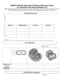
Population and sample
Data are based on one sample
Data of different samples vary
Conclusions are valid for a population
draw conclusion for
population mean
●
●
●
sample:
●
●
mean x
●
●
●
●
●
population mean µ
Master of Science in Medical Biology
4 / 31
Population and sample (II)
Population
The population is the totality of all individuals for which conclusions
should be made.
Sample
A sample of a population is the set of individuals that are actually
observed.
Example:
Population = all human beings (all Swiss citizens)
Sample = students of Medical Biology visiting this lecture
Master of Science in Medical Biology
5 / 31
Recommended literature
Held L., Rufibach K. and Seifert B. (2013). Medizinische Statistik. Konzepte, Methoden,
Anwendungen. Pearson Studium.
- covers simple to most recent advanced statistics, 448 pages.
Kirkwood, B. R. and Sterne, J. A. C. (2006). Essential Medical Statistics. Blackwell, 4th
edition.
- extensive textbook, 502 pages.
H¨
usler, J. and Zimmermann, H. (2006). Statistische Prinzipien f¨
ur medizinische Projekte.
Hans Huber, Bern.
- clearly presented textbook, 355 pages.
Armitage, P., Berry, G., and Matthews, J. N. S. (2002). Statistical methods in medical
research. Blackwell, 4th edition.
- comprehensive textbook, 817 pages.
Johnson, R. A. and Bhattacharyya, G. K. (2001). Statistics. Principles and methods.
Wiley, 4th edition.
- light reading textbook, 236 pages.
Bland, M. (1995). An introduction to medical statistics. Oxford Medical Publications.
- very good introduction with many examples and exercises, 396 pages.
Master of Science in Medical Biology
6 / 31
Biostatistics
Univariate descriptive statistics
Burkhardt Seifert & Alois Tschopp
Department of Biostatistics
Epidemiology, Biostatistics and Prevention Institute (EBPI)
University of Zurich
Master of Science in Medical Biology
7 / 31
Univariate descriptive statistics
Approach “descriptive”, without “significance”
Main types of data (scale types)
Description of data
- via tables
- via graphics
- via location- and dispersion statistics
Master of Science in Medical Biology
8 / 31
Data in a table
In 2006, 245 students (16 groups) of the 2nd semester in
medicine reported their body height and measured their
hand length
sex
height
hand
group
tutor
gender
1
0
1
1
1
0
1
0
0
0
...
168.0
183.5
170.0
159.0
165.0
180.0
181.0
193.0
183.0
183.0
...
17.5
21.0
20.0
17.0
18.0
20.0
19.5
21.5
19.5
20.5
...
1
1
1
1
1
1
1
1
1
1
...
1
1
1
1
1
1
1
1
1
1
...
f
m
f
f
f
m
f
m
m
m
...
Master of Science in Medical Biology
9 / 31
Main types of data
sex
height
hand
group
tutor
gender
1
0
1
1
1
0
1
0
0
0
...
168.0
183.5
170.0
159.0
165.0
180.0
181.0
193.0
183.0
183.0
...
17.5
21.0
20.0
17.0
18.0
20.0
19.5
21.5
19.5
20.5
...
1
1
1
1
1
1
1
1
1
1
...
1
1
1
1
1
1
1
1
1
1
...
f
m
f
f
f
m
f
m
m
m
...
Frequency
%
Cum. %
m
f
106
139
43.3
56.7
43.3
100.0
Total
245
100.0
1) nominal, categorical data
Assignment to categories
→ Counts and % meaningful
Examples: Gender, blood type
Levels
sex
1-2) ordinal data (ordered categorical)
have a ranking
Example: Severity of a disease
Master of Science in Medical Biology
10 / 31
Describing data in tables and graphics
Discrete data
relative frequency =
number of times an event occurred
total number of events
Example: Proportion of blood types in a healthy population
Blood type
Table
Frequency
0
A
B
AB
2313
2678
731
365
Total
6087
Rel. frequency
38
44
12
6
%
%
%
%
100 %
Graphics are:
- easy to comprehend
- easy to create nowadays
Master of Science in Medical Biology
11 / 31
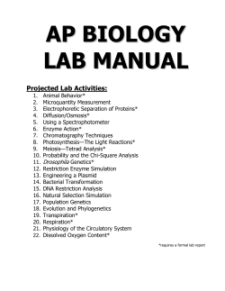
Graphics
Pareto or bar chart
2500
Pie chart
Blood type
1500
500
6%
1000
Counts
2000
0
A
B
AB
38%
44%
0
12%
0
A
B
AB
Blood type
Origin!
Master of Science in Medical Biology
12 / 31
Bar chart
20
Tutor
1
2
3
Percent
15
10
5
0
f
Master of Science in Medical Biology
m
13 / 31
Bar chart
20
Tutor
1
2
3
Percent
15
10
5
0
f
m
Don’t trust a graphic which is higher than wide.
Master of Science in Medical Biology
14 / 31
Bar chart
Tutor
20
1
2
3
Percent
18
16
14
12
10
f
m
Don’t trust a graphic which is higher than wide.
Pay attention to the origin.
Master of Science in Medical Biology
15 / 31
Main types of data
2) continuous (numeric) data
Differences and means meaningful
Example: Temperature in ◦ C
If a absolute zero point exists
→ Ratios meaningful
Examples: Temperature in K,
body height, length of hand
sex
height
hand
group
tutor
gender
1
0
1
1
1
0
1
0
0
0
...
168.0
183.5
170.0
159.0
165.0
180.0
181.0
193.0
183.0
183.0
...
17.5
21.0
20.0
17.0
18.0
20.0
19.5
21.5
19.5
20.5
...
1
1
1
1
1
1
1
1
1
1
...
1
1
1
1
1
1
1
1
1
1
...
f
m
f
f
f
m
f
m
m
m
...
Not meaningful: “There were times when the temperature was 60%
higher than nowadays” BBC 2006
Now
◦
14 C
57 ◦ F
287 K
Then
22 ◦ C
91 F = 33 ◦ C
459 K = 186 ◦ C
◦
Master of Science in Medical Biology
16 / 31
Histogram
Graphical visualisation of the data distribution, “data density”
Continuous and ordinal data
Group data into similar, non overlapping classes (intervals)
Determine number of observations in interval
number of observations in interval
Relative frequency
=
total number of observations
in interval
Density
0.00 0.01 0.02 0.03 0.04 0.05 0.06
Show relative (or absolute) frequencies of intervals in a bar chart
150
Master of Science in Medical Biology
155
160
165
170
175
Body height (in cm)
180
185
17 / 31
Female body height
ordered
Interval
Height
n
150-154
150
153
154
156
156.5
157
158
159
160
161
162
163
164
165
167
168
169
170
171
172
173
174
175
176
177
178
179
180
181
182
183
1
1
1
3
1
2
4
2
8
6
5
5
7
16
8
12
6
14
2
4
9
4
2
4
2
3
1
1
2
2
1
155-159
160-164
165-169
170-174
175-179
180-184
Total
Master of Science in Medical Biology
# Observations
Relative frequency
3
2%
12
9%
31
22%
42
30%
33
24%
12
9%
6
139
4%
100%
18 / 31
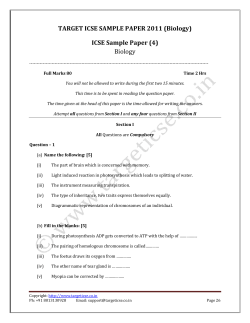
Histogram
0.06
0.04
Density
0.00
0.02
0.04
0.00
0.02
Density
0.06
0.08
f
0.08
m
150
160
170
180
190
200
150
Body height (in cm)
160
170
180
190
200
Body height (in cm)
Shows the distribution in the sample
Meaningful interval length: 5 cm
Fitted a “Gaussian normal distribution” to distribution in
population
Master of Science in Medical Biology
19 / 31
Histogram
0.08
0.00
0.04
Density
0.08
0.00
0.04
Density
0.12
f
0.12
m
150
160
170
180
190
200
150
Body height (in cm)
160
170
180
190
200
Body height (in cm)
Interval length: 1 cm (very variable)
Statement depends mainly on bin width and slightly on center
Histograms are simple and popular, but there are better density
estimators
Master of Science in Medical Biology
20 / 31
Cumulative histogram
A cumulative histogram estimates the distribution function
Empirical distribution function
1.0
0.8
0.6
0.4
Distribution function
0
0.0
0.2
100
60
20
Frequency
140
Cumulative histogram
150
155
160
165
170
175
180
185
150
155
Body height
160
165
170
175
180
Body height
n:139 m:0
Master of Science in Medical Biology
21 / 31
Characterization of the centre of the data
What is a typical, mean value?
Mean x¯: measure of the “middle” (mean, average) value
x¯ = (x1 + x2 + . . . + xn )/n
The mean is the value which balances the data on a set of scales.
0
500
1000
1500
2000
2500
With normally distributed data the mean in a sample is the best fit
to the mean in the population.
sensitive to outliers
Master of Science in Medical Biology
22 / 31
Dispersion or variation of a sample
Master of Science in Medical Biology
23 / 31
Dispersion or variation of a sample
How dispersed are the data around the mean
position?
Variance s 2 :
Compute deviations (x1 − x¯), . . . , (xn − x¯)
Mean? No - would result to be 0!
⇒ s 2 = {(x1 − x¯)2 , . . . , (xn − x¯)2 }/(n − 1)
Note: s 2 in squared units (e. g. cm2 )
√
Standard deviation (SD): s = variance (in cm)
For normally distributed data are 68% of the data in the interval
mean ± SD, 95% of the data in the interval mean ± 2 SD.
sensitive to outliers
no interpretation for non-normally distributed data
Master of Science in Medical Biology
23 / 31
Descriptive statistics
Data are often represented by the mean plus-minus the standard
deviation (mean ± SD).
R-output summary():
f
m
Min.
150.0
165.0
1st Qu.
163.0
176.0
Median
167.0
180.0
Mean
167.2
180.2
3rd Qu.
171.5
184.0
Max.
183.0
197.0
R-output tableContinuos() (“reporttools”, v.1.0.4):
Gender
f
m
N
139
106
Min
150
165
Q1
163
176
Median
167
180
Mean
167.2
180.2
Q3
171.5
184.0
Max
183
197
SD
6.6
6.2
IQR
8.5
8.0
#NA
0
0
Mean ± SD or Mean ± SEM ?
The standard error of the mean (SEM) is the standard
√
deviation of the mean: SEM = SD/ n.
In descriptive statistics the SEM should not be used!
Master of Science in Medical Biology
24 / 31
100
Error bars show mean +/- 1.0 SD
Bars show means
0
50
Height
150
200
Bar chart
m
f
Gender
Bars stand on the floor, therefore pay attention to the origin
Take care of 3-dimensional graphics
Master of Science in Medical Biology
25 / 31
Bar chart
Bars stand on the floor, therefore pay attention to the origin
Take care of 3-dimensional graphics
Master of Science in Medical Biology
26 / 31
175
●
Error bars show mean +/- 1.0 SD
Dots show means
170
Height
180
185
Dot charts
160
165
●
m
f
Gender
The origin has no meaning here
Master of Science in Medical Biology
27 / 31
Percentiles (quantiles)
α.– percentile (α% – quantile):
α% of the data are smaller than or equal to the α. – percentile
and (100 − α)% are larger or equal.
Median = 50. percentile
Examples:
Quartile = 25. and 75. percentiles
1.0
Distribution function
0.8
0.6
0.4
0.2
0.0
150
160
170
180
190
200
Body height
Not unique!
In R there are nine different quantile algorithms.
Master of Science in Medical Biology
28 / 31
Percentiles (quantiles)
α.– percentile (α% – quantile):
α% of the data are smaller than or equal to the α. – percentile
and (100 − α)% are larger or equal.
Median = 50. percentile
Examples:
Quartile = 25. and 75. percentiles
1.0
0.6
0.5
●
0.4
Median
Distribution function
0.8
0.2
0.0
150
160
170
180
190
200
Body height
Not unique!
In R there are nine different quantile algorithms.
Master of Science in Medical Biology
28 / 31
Percentiles (quantiles)
α.– percentile (α% – quantile):
α% of the data are smaller than or equal to the α. – percentile
and (100 − α)% are larger or equal.
Median = 50. percentile
Examples:
Quartile = 25. and 75. percentiles
1.0
0.75
●
0.6
0.5
●
●
3. Qu.
0.25
0.2
Median
0.4
1. Qu.
Distribution function
0.8
0.0
150
160
170
180
190
200
Body height
Not unique!
In R there are nine different quantile algorithms.
Master of Science in Medical Biology
28 / 31
Percentiles (quantiles)
α.– percentile (α% – quantile):
α% of the data are smaller than or equal to the α. – percentile
and (100 − α)% are larger or equal.
Median = 50. percentile
Examples:
Quartile = 25. and 75. percentiles
1.0
0.75
●
0.6
0.5
●
●
3. Qu.
0.25
0.2
Median
0.4
1. Qu.
Distribution function
0.8
IQR
0.0
150
160
170
180
190
200
Body height
Not unique!
In R there are nine different quantile algorithms.
Master of Science in Medical Biology
28 / 31
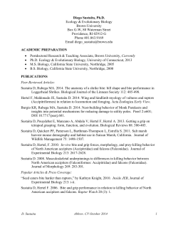
Boxplot
190
●
0
170
160
Height
180
maximum (without outliers)
upper quartile
median
lower quartile
150
minimum (without outliers)
●
m
f
Gender
Master of Science in Medical Biology
29 / 31
Characterization of the centre of the data
Median: centre of the data, 50. precentile
i.e. half of the sample is above the median, the other half below
The median is robust to outliers.
Mode: (rarely used)
- discrete data: most frequent value
- continuous data: maximum of the density
(population only)
Master of Science in Medical Biology
30 / 31
Dispersion of a sample
Range = maximum − minimum
- states the range of all values in the sample
- strongly influenced by outliers
- but: Minimum and maximum are easy to understand
Interquartile range (IQR)
= 75. percentile − 25. percentile
= length of box in the boxplot, contains central 50% of data
- as standard deviation a measure for the magnitude of the
central range of the data
With normally distributed data half the IQR equals 0.67 SD.
- “Median(IQR)” tells nothing about skewness
⇒ Data are often reported as
“Median [lower quartile, upper quartile]”.
Master of Science in Medical Biology
31 / 31