
Technical Description of the Health and Retirement Survey Sample Design
PUBLIC USE VERSION
Technical Description of the
Health and Retirement Survey Sample Design
Steven G. Heeringa
Judith H. Connor
Sampling Section
Institute for Social Research
University of Michigan
Ann Arbor, MI
May 1995
May 16, 1995
TECHNICAL DESCRIPTION
HEALTH AND RETIREMENT STUDY
SAMPLE DESIGN
The following technical memorandum describes the sample design, sampling procedures, and
sample outcomes for Wave 1 of the Health and Retirement Study (HRS). This document is divided
into six sections. The introduction describes the purpose and organization of the HRS. Sections 2
and 3 provide an overview and a detailed description of the multi-stage area probability sample
design. The fourth section reports the HRS Wave 1 sample outcomes -- a comparison of the
expected versus observed occupancy, eligibility, and response rates. Sections 5 and 6 contain
descriptions of the construction and use of the analysis weights and the codes and procedures for
computation of sampling errors for the HRS data.
1. INTRODUCTION
The HRS is funded by the National Institute on Aging (NIA) through a special Congressional
appropriation. Although the initial HRS funding was for five years beginning in March 1991, the
study is expected to continue for at least 10-12 years and possibly longer. The initial five year
funding included a planning year and two data collections, April - December 1992 (Wave 1) and
April - December 1994 (Wave 2).
Dr. F. Thomas Juster at the Institute for Social Research (University of Michigan) is the
Principal Investigator for this national program of research. In addition, more than thirty researchers
and professionals from the ISR and other universities and government agencies have collaborated on
the HRS study design and content.
As the proportion of the population living to retirement and beyond increases, it is important
for policy makers to understand the changing needs of that population in order to guide planning and
policy decisions. There has been no extensive research on factors influencing or resulting from
retirement since the Longitudinal Retirement History Survey conducted by the Bureau of the Census
and the Social Security Administration during the period of 1969 - 1979. The HRS is intended to
provide policy-makers with up-to-date information on changes in retirement and disability patterns,
and to provide scientists with data to generate more accurate and realistic models of the retirement
decision and the economic and health causes and consequences of retirement and aging.
HRS is designed to collect information on persons from pre-retirement into retirement.
Wave 1 questionnaire content concentrated on the economic, health, and other factors that influence
retirement decisions. As the HRS panel ages, future waves of data collection will emphasize health
status and economic well-being.
1
2. SAMPLE DESIGN OVERVIEW
2.A. Study Population
The target population for Wave 1 of the HRS includes all adults in the contiguous United
States, aged 51 - 61 (born during the years 1931 - 1941), who reside in households. Following
conventional practice for population surveys, institutionalized persons (prisons, jails, nursing homes,
long-term or dependent care facilities) are excluded from the survey population.
HRS uses a national area probability sample of U.S. households with supplemental
oversamples of Blacks, Hispanics and residents of the state of Florida. The majority of the sample
population is approaching retirement or already retired, but the sample also includes individuals who
are not currently working or who have never worked outside the home.
The HRS observational unit is an eligible household financial unit. The HRS household
financial unit must include at least one age-eligible member from the 1931-1941 birth year cohorts:
1) a single unmarried age-eligible person; 2) a married couple in which both persons are age eligible;
or 3) a married couple in which only one spouse is age eligible. Throughout this document, the
convenient term "household" will be used interchangeably with the more precise "household
financial unit" definition. For most HRS-eligible households, the terms are interchangeable.
However, the reader should note that some households may contain multiple household financial
units. If a sample housing unit (HU) contains more than one unrelated age-eligible person (i.e.,
financial unit), one of these persons is randomly selected as the financial unit to be observed. If an
age-eligible person has a spouse, the spouse is automatically selected for HRS even if he or she is
not age-eligible. Based on the 1991 Current Population Survey, about 19.2% of U.S. households
were expected to be eligible for HRS. Of these about 35.9% were expected to be single-person
household financial units and 64.1% were expected to be married-couple household financial units
(including households in which a respondent is living with a partner in a marriage-like relationship).
Both partners were expected to be age-eligible in 49.6% of the eligible households with a
married couple; one partner would be less than age 51 in 25.2% of the eligible married couple
households; and one partner would be older than 61 in 25.2% of the eligible married couple
households.
2.B. Multi-stage Area Probability Sample Design
The HRS sample is selected under a multi-stage area probability sample design. The sample
includes four distinct selection stages. An overview of these selection stages is given here. For a
more detailed discussion, see Section 3. The primary stage of sampling involves probability
proportionate to size (PPS) selection of U.S. Metropolitan Statistical Areas (MSAs) and non-MSA
counties. This stage is followed by a second stage sampling of area segments (SSUs) within
sampled primary stage units (PSUs). The third stage of sample selection is preceded by a complete
listing (enumeration) of all housing units (HUs) that are physically located within the bounds of the
selected SSU. The third sampling stage is a systematic selection of housing units from the HU
listings for the sample SSUs. The fourth and final stage in the multi-stage design is the selection of
the household financial unit within a sample HU.
2
3
2.C. Oversamples of Special Populations
In addition to the nationally-representative, multi-stage area probability sample (the core
sample), the HRS design includes three oversamples. The oversamples are introduced as
supplements to the core national sample and are designed to increase the numbers of Black and
Hispanic HRS respondents as well as the number of HRS respondents who are residents of the state
of Florida. Sampling weights are provided on all HRS data sets to compensate for the unequal
probabilities of selection between the core and oversample domains (see Section 5).
1990 Census data suggest that the expected total of completed interviews from an equal
probability sample of U.S. households would contain approximately 10% age-eligible Black
households. Within the 84 PSUs which comprise the first stage of the SRC National Sample Design,
a supplemental sample of SSUs (area segments) was selected from second stage strata of Census
block groups containing 10% or more 1990 Census households with a Black head. Thus, eligible
persons in residential areas eligible for the second stage sample supplement (more than 10% Black
households per block group) have a greater probability of selection than persons in areas which have
less than 10% Black households. Through the use of this procedure, the representation of eligible
Black household units was expected to increase from 10% to about 18.6% of the total HRS sample.
For an equal probability sample of U.S. households, estimates from the Current Population
Survey would suggest that 5% of the HRS households would include a respondent of Hispanic
origin. Approximately 58% of these Hispanic households are of Mexican ancestry. The design
objective for the HRS was to obtain a two-fold oversampling of Mexican-American households.
The Hispanic supplement required additions to the PSU sample, especially in the West and
Southwest. In addition to expanding the primary stage of the sample, supplemental sampling of
SSUs in areas with Hispanic household density of 10% or more was used to assure sufficient sample
size to permit subgroup analysis. The Hispanic supplement was designed to increase the
representation of Hispanics, including the Mexican-American subgroup, from 5% to 8.6% of the
total HRS sample.
Table 1 shows the proportion of Black and Hispanic households expected from an equal
probability sample of U.S. households and the proportion expected from the HRS special allocation.
Table 1: HRS Special Sample Allocation Compared to Proportionate Allocation (HHs)
Household
Racial / Ethnic
Group
% Households
Proportionate
Allocation
% Households
HRS Allocation
Blacks
10.0%
18.6%
Hispanics
5.0%
8.6%
All Others
85.0%
72.8%
TOTAL
100.0%
100.0%
4
In addition to the oversamples of Black and Hispanic households, the HRS design
incorporates a two-fold oversample of Florida households (across all race and ethnic groups).
Supplemental funds were obtained to increase the number of Florida PSUs (from 5 to 12 Florida
PSUs). This insured that there would be sufficient precision to allow separate state-level analysis of
data from the HRS Florida respondents. The HRS multi-stage area probability design for the core
sample and supplements is described in detail in Section 3.
2.D. Integrated Design and Procedures: Core Sample and Supplements
The HRS core sample and special supplemental samples are integrated within the general
framework of the SRC National Sample design. In expanding the PSU samples for both the Florida
and Hispanic supplemental samples, the 84 strata SRC design was used as the framework. In
Florida, the five original National Sample strata were subdivided to form 12 new Florida strata -- six
of which became self-representing for the HRS Florida sample. Similarly, the original National
Sample stratification was reorganized and used in selecting additional Hispanic PSUs. These
Hispanic PSUs are new or additional primary-stage selections from the original SRC strata which
had significant Mexican-American population.
The HRS Black supplement sample is also selected within the SRC National Sample
stratification. The Black supplement required no added PSU selections beyond those included in the
full SRC National Sample. The Black supplement SSUs are selected from the original National
Sample PSUs. The HRS primary stage sample does use the full set of National Sample PSUs
(instead of the 2/3 set of PSUs) in the South, the Region which accounts for 52.8% of the U.S. Black
population (34.4% of total U.S. population).
The use of sampling weights which compensate for the oversampling of the three domains
allows the core and supplement samples to be combined in analyses. The sampling weights are
incorporated into the analysis weights (described in Section 5).
5
3. SAMPLE DESIGN AND PROCEDURES: MULTI-STAGE AREA PROBABILITY
SAMPLE DESIGN
The HRS core sample and special supplements comprise an integrated sample of the U.S.
household population. Each multi-stage component of the HRS area probability sample is consistent
with the general sample design framework and sampling procedures of the SRC National Sample
(Heeringa, Connor, and Darrah, 1984).
The HRS sample was selected at a time when 1990 Census data were just becoming
available. For this reason some features of the design (e.g., PSU definitions) are consistent with
1980 Census definitions. However, other features such as the geographic definitions of SSUs and
the measures of size (MOS) for SSUs were updated to take best advantage of newly released Census
mapping materials (TIGER) and 1990 Census counts of population and housing.
3.A. Primary Stage Selection
3.A.1. Core Sample
The selection of core SRC National Sample primary stage sampling units (PSUs), which
depending on the sample stratum are either SMSAs (MSAs),1 single counties or groups of small
counties, was based on the county-level 1980 Census Reports of Population and Housing and the
1980 SMSA definitions. National Sample PSUs were assigned to 84 explicit strata based on
MSA/non-MSA status, PSU size and geographic location. Sixteen of the 84 National Sample strata
contain only a single self-representing (SR) PSU, each of which is included with certainty in the
primary stage of sample selection. The remaining 68 nonself-representing (NSR) strata contain
more than one PSU. From each of these nonself-representing strata, one PSU was sampled with
probability proportionate to its size (PPS) measured in 1980 Census occupied housing units.
The full 1980 SRC National Sample design of 84 primary stage selections was designed to be
1
SMSAs or Standard Metropolitan Statistical Areas are now called MSAs (Metropolitan Statistical Areas) or PMSAs
(Primary Metropolitan Statistical Areas). PMSAs are part of larger CMSAs (Consolidated Metropolitan Statistical
Areas) while MSAs are not part of CMSAs. The PSUs in the 1980 SRC National Sample used 1980 SMSA definitions.
These definitions can be found in the publication, 1980 Census of Population. Standard Metropolitan Statistical Areas:
1980 (PC80-S1-5; issued October 1981). The following definition is found on page 4 of the above mentioned
publication: SMSAs are "designated as Federal statistical standards by the Office of Management and Budget (OMB) to
maintain geographic consistency in the presentation of data issued by Federal agencies. The general concept of an
SMSA is one of a large population nucleus, together with adjacent communities which have a high degree of economic
and social integration with that nucleus." In this document, the current term, MSA, will be used to refer to both MSAs
and PMSAs.
6
optimal for very large studies. To permit the flexibility needed for optimal design of smaller survey
samples, the primary stage of the SRC National Sample can be partitioned into smaller subsamples
of PSUs. Each of the partitions represents a stratified subselection from the full 84 PSU design
(Heeringa, Connor, Darrah; 1984).
In complex sample designs, the precision of sample estimates is related to a number of
factors, an important one being the number of PSUs which contribute data to the estimate. The basic
sample for the HRS study is selected from the 2/3 partition of the full 84 strata of the 1980 SRC
National Sample. The 2/3 partition includes the 16 self-representing MSA PSUs and a stratified
subsampling of 45 of the 68 nonself-representing PSUs for a total of 61 PSUs. To increase the
precision for estimates based on Black respondent data, the primary stage of the HRS national
sample design includes all Census South Region MSA and non-MSA PSUs (nine additional PSUs).
The Census South Region includes about 34% of the total U.S. population but almost 53% of Black
population.
In addition, the full set of 23 non-MSA PSUs in the SRC National Sample was used for HRS.
The purpose for including the full set of 23 non-MSA PSUs in the HRS design was to achieve
improved precision of HRS analyses for rural populations. Since the selection of National Sample
PSUs is performed independently within Census regions, the use of the full sample in the South and
non-MSA strata and the 2/3 sample in the Northeast, Midwest, and West nonself-representing MSA
strata does not bias the sample for non-Black households. Under the standard multi-stage sample
procedure, an adjustment for the larger PSU sample in the South and non-MSA strata -- i.e., smaller
samples of HUs per PSU -- enters at a subsequent stage of the selection process. Including the added
PSU selections for the Hispanic Supplement and Florida sample, the HRS sample has 93 primary
stage selections: 27 self-representing and 66 nonself-representing.
3.A.2. Black Supplement
Although no additional PSU selections were made for the HRS Black supplement, the
decision to use the full instead of the 2/3 set of National Sample PSUs in the South was made in
order to increase the precision of survey estimates from the subsample of Black HRS respondents.
3.A.3. Hispanic Supplement
The HRS Hispanic supplement sample required additions to both the primary and secondary
stages of the basic SRC National Sample design. At the primary stage, the supplement involved a
restratification of the 84 strata of the 1980 SRC National Sample to reflect the distribution of the
U.S. Mexican-American Hispanic population. The restratification was performed through simple
recombinations of previously defined SRC National Sample strata. As shown in Table 2, the 84
1980 National Sample strata were reorganized to create 34 collapsed primary stage strata for the
HRS Hispanic supplement. A total of a=23 Hispanic supplement PSU selections were allocated to
these 34 collapsed strata based on 1990 Census counts of Mexican-American Hispanic households
for PSUs assigned to the redefined strata. Column 4 of Table 2 shows the 1990 Census measures of
size (MOS) for each of the recombined strata. Many of the recombined strata such as stratum 1, the
New York, NY MSA, contain very few Mexican-American households, and no supplemental PSU
selections were added to these strata. Other strata (e.g., Medium California MSAs) contain large
Mexican-American populations and therefore multiple supplemental Hispanic PSUs are allocated to
such strata. The majority of Hispanic PSUs are in the Southwest and West. Five of the 16 SRC
7
National Sample self-representing PSUs were included with certainty in the Hispanic supplement:
Los Angeles CA; Chicago IL; San Francisco CA; Dallas TX; and Houston TX.
Eight of the 23 Hispanic supplement PSUs are NSR PSUs in the SRC National Sample
design. The remaining 10 Hispanic supplement NSR PSUs are new PSU selections not previously
selected as part of the SRC National Sample.
By definition, the Hispanic supplement SR PSUs were the only PSUs in their stratum.
Therefore, the five SR PSUs which had significant Mexican-American Hispanic population were
automatically included in the Hispanic supplement.
In the Hispanic supplement NSR strata with sufficient Mexican-American Hispanic
population, the core PSUs were not automatically selected for the Hispanic supplement. The KishScott procedure (Kish, 1963) was used to maximize the probability of reselection of the core PSUs in
the Hispanic supplement. In some cases, a new Hispanic PSU replaced the National Sample PSU in
the Hispanic supplement. In other cases, the National Sample PSU was retained for the supplement.
Additional new Hispanic supplement PSUs were also selected in strata which had a proportionately
high Mexican-American population.
8
Table 2: Allocation of Hispanic PSUs and SSUs to SRC National Sample Strata
and Definition of Mexican-American Strata
Hisp.
Supp.
Str.
No.
Natl.
Smpl.
Str.
No.
National Sample
Stratum
Stratum MOS
(1990 Mex.-Amer.
population)
No. 1st
Stage
Selectns.
No. 2nd
Stage
Selectns.
Self-Representing Strata
1
1
New York, NY
73,529
0
2
2
Los Angeles, CA
2,527,160
1
28
3
3
Chicago, IL
574,847
1
7
4
4
Philadelphia, PA
11,973
0
5
5
Detroit, MI
50,801
0
6
6
San Francisco, CA
298,895
1
7
7
Washington, DC
28,008
0
8
8
Dallas, TX
449,218
1
5
9
9
Houston, TX
599,115
1
7
10
10
Boston, MA
8,226
0
11
11
Nassau-Suffolk, NY
5,561
0
12
12
St. Louis, MO
13,004
0
13
13
Pittsburgh, PA
3,963
0
14
14
Baltimore, MD
5,965
0
15
15
Minneapolis, MN
23,026
0
16
16
Atlanta, GA
22,654
0
4
Nonself-Representing MSA Strata
17
17-24
MSAs in EAST
59,944
0
18
25-35
MSAs in MIDWEST
335,944
0
19
36-43
MSAs in AL,FL,GA,
LA,MS,SC
158,155
0
20
44
Large TX MSAs
1,579,046
3
9
18
Table 2, continued
Hisp.
Supp.
Str.
No.
Natl.
Smpl.
Str.
No.
National Sample
Stratum
21
45
Small TX MSAs
617,233
1
22
46-51
MSAs in AR,DE,KY,
MD,NC,OK,TN,TX,
VA,WV
108,153
0
23
52
San Diego, CA
449,541
1
5
24
53-54
Large MSAs in WA,
OR,North CA
320,861
1
4
25
55
Sacramento, CA and
Denver, CO
280,792
1
3
26
56-57
Medium California
MSAs
1,427,032
3
18
27
58
Small CA MSAs
774,697
2
12
28
59-61
Non-California in
WEST (except Seattle
WA, Portland OR,
Denver CO, Honolulu
HI, Anchorage AK
937,721
2
12
Stratum MOS
(1990 Mex.-Amer.
population)
No. 1st
Stage
Selectns.
No. 2nd
Stage
Selectns.
7
Nonself-Representing Non-MSA Strata
29
62-64
Non-MSAs in
NORTHEAST
8,461
0
30
65-71
Non-MSAs in
MIDWEST
155,878
0
31
72-75
Non-MSA counties in
AL,FL,GA,LA,MS,
SC
158,384
0
32
76
TX & OK Non-MSA
Counties
570,451
1
33
77-81
Non-MSA counties in
AR,DE,KY,MD,NC,
OK,TN,VA,WV
47,072
0
10
6
Table 2, continued
Hisp.
Supp.
Str.
No.
34
Nat.
Smpl.
Str.
No.
82-84
National Sample
Stratum
Stratum MOS
(1990 Mex.-Amer.
population)
Non-MSA counties in
WEST
TOTAL:
No. 1st
Stage
Selectns.
No. 2nd
Stage
Selectns.
806,783
3
14
13,492,093
23
150
3.A.4. Florida Oversample
Five of the 84 strata in the SRC National Sample include only Florida MSAs or non-MSA
counties. In order to allow sufficient precision for separate analysis of data from Florida
respondents, more Florida PSUs were required for HRS. To accomplish this, the five Florida
National Sample strata were subdivided to form 12 strata. Six of these new strata include a single
self-representing PSU. Five of the 12 new strata retained the PSU used in the 1980 SRC National
Sample. Retaining the original National Sample PSU selections in five of 12 new Florida strata
greatly reduced the cost of relocating or training new field staff. Table 3 shows the definition of the
12 Florida strata.
As seen in Table 3, Florida strata 1 - 6 were created from the SRC National Sample strata 40,
41, and 42. In order to determine the size of the six new Florida NSR strata, the total housing units
in the six Florida SR strata were subtracted from the total housing units in the state, and the
remainder was divided by six. The result of this calculation was 404,129 -- the target number of
housing units for the remaining NSR strata. Table 3 shows that the Florida NSR stratum sizes vary
about this target -- from a low of 359,814 to a high of 466,391.
Florida strata 7 - 10 were created from the SRC National Sample stratum 43. The MSAs in
this stratum were grouped together by geographic area into four strata of roughly equivalent numbers
of housing units (as shown in Table 3). The original National Sample PSU for stratum 43 was
retained. In addition, three new PSUs were selected with PPS from the remaining three Florida
strata.
Florida strata 11 and 12 were created from National Sample stratum 75. Stratum 75 was
divided geographically into Florida stratum 11 (in the north) and Florida stratum 12 (in the south).
Each stratum contained four counties which had at least 40 percent of their population aged 55 or
older. One PSU was selected by PPS from the NSR PSUs in Florida stratum 11. Another was
selected by PPS from the NSR PSUs in Florida stratum 12.
11
Table 3: Florida Supplement Restratification
FL
Str.
No.
National
Sample
Str. No.
National Sample Stratum
Stratum MOS
(1990 HUs)
Self-Representing MSAs
1.
40-41
Large Florida MSA
975,046
2.
40-41
Large Florida MSA
771,288
3.
40-41
Large Florida MSA
628,660
4.
42
Medium Florida MSAs
461,665
5.
42
Medium Florida MSAs
448,490
6.
42
Medium Florida MSAs
390,335
Nonself-Representing MSAs
7.
43
Small Florida MSAs
366,122
8.
43
Small Florida MSAs
461,351
9.
43
Small Florida MSAs
359,814
10.
43
Small Florida MSAs
361,541
Nonself-Representing Non-MSAs
11.
75
Florida non-MSA counties in
southern part of state
409,559
12.
75
Florida non-MSA counties in
northern part of state
466,391
12
3.B. Secondary-Stage Selection of Area Segments
3.B.1. Core Sample
3.B.1.a. SSU Stratification and Selection
The second stage of the HRS core sample component was selected directly from
computerized files that were prepared from the 1990 Census PL 94-171 CD-ROM file. The
designated second-stage sampling units (SSUs) or "area segments" are comprised of Census blocks
or groups of blocks. Each SSU was assigned a measure of size equal to the total 1990 housing unit
count for the area. A minimum of 72 housing units was required for core sample SSUs. If a block
had no housing units or fewer than 72 housing units, it was linked with adjacent blocks to form
SSUs of sufficient size.
Prior to selection, Census blocks within each PSU were implicitly stratified by geography.
Counties within MSA PSUs having more than one county were ordered by size and distance from
the center of the MSA. This ordering was accomplished by placing the county with the central city
first, suburban counties next, and remaining counties last in a circular pattern. In non-MSA PSUs
comprised of more than one county, the Census blocks were ordered by county according to
geographic location and population size of the county. Within counties, the Census blocks were
sorted in Census tract order and within tract by Census block number. The numerical ordering of
Census tracts and blocks corresponds closely to the geographic location within the county,
SSU selection was performed with probabilities proportionate to the assigned housing unit
measures of size. A computer program developed at SRC was used to group the ordered file of
Census blocks into SSUs of minimum measure of size (72 housing units) and to perform a
systematic selection of the SSUs.
3.B.1.b. SSU Allocation
The number of SSUs allocated to sample PSUs depends on the population size of the stratum
which the PSU represents. The number of SSUs in the self-representing PSUs is proportional to the
size of the PSU (stratum) and ranges from a high of 61 in New York to a low of 16 in the six
smallest SR PSUs. Table 4 shows the number and type of core sample SSUs in each PSU. In
addition to showing the core allocation, the table shows the allocation of Black and Hispanic
supplement SSUs (described in the following sections).
13
Table 4: HRS SSU Allocation by National Sample Stratum
National
Sample
Str. No.
Total
HRS
SSUs
Core
Sample
SSUs
Black
Suppl.
SSUs
Hispanic
Suppl.
SSUs
1
75
61
14
---
2
85
50
7
28
3
60
43
10
7
4
35
29
6
---
5
34
27
7
---
6
31
24
3
4
7
27
20
7
---
8
31
23
3
5
9
35
25
3
7
10
19
18
1
---
11
17
16
1
---
12
19
16
3
---
13
17
16
1
---
14
19
16
3
---
15
17
16
1
---
16
19
16
3
---
17
27
24
3
---
18
29
24
5
---
21
27
24
3
---
23
28
24
4
---
24
24
24
---
---
26
27
24
---
---
27
28
24
4
---
28
27
24
3
---
29
24
24
---
---
31
24
24
---
---
32
25
24
1
---
14
Table 4, continued
National
Sample
Str. No.
Total
HRS
SSUs
Core
Sample
SSUs
Black
Suppl.
SSUs
Hispanic
Suppl.
SSUs
33
24
24
---
---
34
28
24
4
---
36
21
18
3
---
37
18
12
6
---
38
16
12
4
---
39
24
18
6
---
40
27
24
3
---
41
25
24
1
---
42
27
24
3
---
43
27
24
3
---
44
24
18
---
6
45
21
18
3
---
46
12
12
---
---
47
18
18
---
---
48
13
12
1
---
49
19
18
1
---
50
22
18
4
---
51
16
12
4
---
52
5
---
---
5
53
24
24
---
---
55
27
24
---
3
56
30
24
---
6
57
30
24
---
6
58
30
24
---
6
59
24
24
---
---
60
30
24
---
6
62
6
6
---
---
15
Table 4, continued
National
Sample
Str. No.
Total
HRS
SSUs
Core
Sample
SSUs
Black
Suppl.
SSUs
Hispanic
Suppl.
SSUs
63
12
12
---
---
64
12
12
---
---
65
12
12
---
---
66
12
12
---
---
67
6
6
---
---
68
12
12
---
---
69
6
6
---
---
70
12
12
---
---
71
6
6
---
---
72
10
6
4
---
73
16
12
4
---
74
15
12
3
---
75
12
12
---
---
76
12
12
---
---
77
18
12
6
---
78
12
12
---
---
79
6
6
---
---
80
12
12
---
---
81
16
12
4
---
82
12
12
---
---
83
8
6
---
2
84
12
12
---
---
85
12
12
---
---
86
12
12
---
---
87
12
12
---
---
88
18
18
---
---
89
12
12
---
---
16
Table 4, continued
National
Sample
Str. No.
Total
HRS
SSUs
Core
Sample
SSUs
Black
Suppl.
SSUs
Hispanic
Suppl.
SSUs
90
12
12
---
---
91
12
12
---
---
92
6
---
---
6
93
6
---
---
6
94
7
---
---
7
95
4
---
---
4
96
6
---
---
6
97
6
---
---
6
98
6
---
---
6
99
6
---
---
6
100
6
---
---
6
101
6
---
---
6
1818
1502
166
150
Total
3.B.2. Black Supplement
At the primary stage of sampling, the Black supplement is fully integrated with the core
National Sample design -- both the core HRS sample and the Black supplement share the same set of
primary stage sample locations. The Black supplement to the HRS consists of 166 additional SSU
selections. However, within each PSU location, the selection of Black Supplement SSUs was
independent of the core SSU selection.
The first step in the sampling process was to allocate the 166 Black supplement SSUs to the
National Sample PSUs. Since the purpose of the Black supplement is to improve the precision of
survey estimates for the Black population, the supplemental sample of SSUs was allocated to the
sample PSUs in proportion to the total Black population of the stratum which each sample PSU
represents. (In a standard national household sample -- such as the HRS core sample -- this
allocation would be proportional to total population or housing counts.) Table 4 shows the SSU
allocation by PSU for the Black supplement.
A special Black supplement frame was then constructed for each PSU which had been
allocated one or more supplemental SSUs. This frame consisted of SSUs having at least ten percent
17
Black population. Through the use of appropriate weights in the analysis of the survey data, Black
households not covered by the supplemental frame (but covered by the core National Sample frame)
will receive unbiased representation in survey estimates. Excluding low density Black areas from
the supplemental frame greatly increases the cost efficiency of the Black supplement.
Because the minimum measure of size for the Black supplement SSUs was based on Black
households, the size of an individual SSU could vary depending on the density of Black households
within its boundaries. Based on the predetermined allocation to the PSUs, the Black supplement
SSUs were selected with probability proportionate to size measured in 1990 Census counts of Black
households. Although the Black Supplement is intended primarily to increase the number of eligible
Black HRS respondents, there is no race screening in the Black supplement SSUs. All households
with at least one person born during the years 1931 - 1941 are eligible regardless of race. However,
the average proportion of Black households in Black supplement SSUs is about 75 percent
(compared to 10 percent in the core SSUs).
3.B.3. Hispanic Supplement
The Hispanic supplement SSUs were selected using the 1990 Census PL 94-171 file. For
each PSU which is part of the Hispanic supplement (see Section 3.A.3), a file was constructed of all
Census blocks which are part of the PSU definition. The file of Census blocks was ordered by
geography (as described in Section 3.B.1.a). A computer program was used to cluster the Census
blocks into SSUs with a minimum measure of size of 96 Hispanic persons. A sampling frame was
then formed from only those SSUs having at least ten percent Hispanic population. From this frame
the predetermined number of SSUs was selected from each Hispanic supplement PSU with
probability proportional to the Hispanic population. The SSU allocation to Hispanic supplement
PSUs is shown in Table 2.
In the Hispanic supplement SSUs, households were screened to include only those which had
at least one eligible Hispanic person. The average proportion of Hispanics in the Hispanic
supplement SSUs was expected to be about 20 percent (versus about 5 percent in the core SSUs).
Although the allocation of the Hispanic supplement PSUs and SSUs was based on MexicanAmerican population, all self-reported Hispanic households were eligible for the Hispanic
supplement. However, because the supplement was concentrated in areas with high MexicanAmerican population density, the Hispanic respondents in the supplement are more likely to be
Mexican-Americans than other groups such as Puerto Ricans or Cuban-Americans.
3.B.4. Florida Sample
The HRS Florida sample is completely integrated with the core sample at both the PSU and
SSU levels. Because of the way the additional Florida PSUs were selected, all twelve Florida PSUs
and all Florida SSUs are part of both the core and special Florida samples. A sampling weight which
compensates for the two-fold oversampling in Florida is required for HRS analyses. The sampling
weights are described in Section 6. Table 4 shows the allocation of SSUs to the Florida PSUs.
18
3.C. Third-Stage Selection of Housing Units
For each SSU selected in the second sampling stage, a listing was made of all housing units
located within the physical boundaries of the segment. For SSUs with a very large number of
expected housing units or a very large geographic area, all housing units in a subselected part of the
SSU were listed. Within each sample domain a final equal probability sample of housing units for
the HRS survey was systematically selected from the housing unit listings for the sampled SSUs.
The equal probability sample of households within each sample domain was achieved by using the
standard multi-stage sampling technique of setting the sampling rate for selected housing units
within SSUs to be inversely proportional to the PPS probabilities used to select the PSU and the
SSU. The number of selected housing unit listings took into account the expected occupancy rate,
the screening required to find age-eligible households, and the expected response rate. These sample
design parameters are discussed in Section 4.
3.D. Fourth-Stage: Respondent Selection
Within each sampled housing unit, the SRC interviewer prepared a complete listing of all
household members. The full name, sex, age, and relationship to informant was recorded for each
member of the household. The informant was then asked the year of birth of any person in the
housing unit aged 50 to 62. If the year of birth was 1931 - 1941 inclusive, the person was eligible to
be interviewed for the HRS survey. If no one in the housing unit was born during that time period,
the household was classified as having no eligible respondent (NER). The HRS area probability
sample housing unit listings were also used to screen for persons born prior to 1924. These
household members would be interviewed for a future SRC study, the Aging and Health in America
(AHEAD) study. The National Institute on Aging sponsored both the HRS and the AHEAD studies.
If the HRS sample household contained only one age-eligible person or if there were two
age-eligible persons who were married/partnered to each other, no respondent selection procedure
was required. The single person or both partners were designated as the financial unit to be
interviewed. If there was more than one age-eligible person and they were not married (or in an
equivalent relationship), an objective procedure described by Kish (1965) was used to select a single
eligible respondent to be interviewed. Regardless of circumstances, no substitutions were permitted
for the designated respondent. If the selected age-eligible person had a spouse, the spouse was also
designated for the HRS person interview whether or not the spouse was age eligible.
An unmarried age-eligible respondent was automatically designated the "R1" or primary
household respondent. In the case of a married couple, the person who considered himself or herself
more knowledgeable about the family's assets, debts, and retirement was designated the "R1"
respondent and the spouse became the "R2" or secondary respondent. In a married couple household
financial unit, the "R1" respondent was not necessarily age eligible.
3.E. HRS Sample Release and Survey Monitoring
Within each PSU, the HRS SSUs were randomly divided into two rotation groups.
Interviewing began in the first rotation of SSUs in April 1992 and in the second set in June 1992.
This staged introduction of SSUs was designed to control sample size and cost.
19
In April 1992, one half of the selected housing units from the first set of SSUs or one-fourth
of the total core sample was released for interviewing. In June 1992, the remaining one-half of the
sample lines in the first set of SSUs and one-half of the sample lines in the second set of SSUs were
introduced. At this point, three-fourths of the sample lines were in the field and one fourth of the
sample was withheld. In September, the third release of sample brought the complete sample into
the field. If the survey costs had been too high or the eligibility higher than expected, the size of the
third release of sample could have been adjusted. This was possible because the entire sample of
housing units was assigned to 24 replicates, each of which was a proper subsample of the whole.
The September release could have used part or all of the available replicates.
Figure 1 shows the timing of the sample release for the various components of the total
sample, i.e., the core sample and the supplemental samples of Blacks and Hispanics as well as the
Florida oversample. Figure 2 shows that the sample release schedule for the total sample produced
an interview completion rate which facilitated monitoring of survey quality and cost factors. From
April to June, interview completions accumulated at a relatively slow rate. Following the major June
sample release, interview completions began to rise more sharply. Immediately prior to the
September release date, about 60 percent of the expected interviews were completed. At that point, a
judgment could be made about the size of the third sample release in September. Because the
eligibility rate was lower than expected, the entire third set of sample was released. The comparison
of survey design parameters with survey outcomes is discussed in Section 4.
20
4. SAMPLE OUTCOMES
4.A. Occupancy Rate, HU Update Rate
As part of routine survey procedure, SRC interviewers updated the housing units listings for
each HRS SSU immediately prior to the start of interview data collection. Two forms of HU listing
update were performed. Type I updating involved a pre-study check of the SSU listing for new or
previously missed HU structures. Type II updating involved the identification of previously
unidentified housing units within listed structures. In designing the sample, it was assumed that the
offsetting effects of Type I and Type II updating (adding sample housing units) and the vacancy rate
would result in 0.90 household contacts for every housing unit sampled. The 0.90 value is the
product of a factor that reflects an expected 3% increase in sample size due to updating and an
estimated occupancy rate of 87.3% (i.e., .90 = 1.03 * .873).
Table 5 shows the update factors and occupancy rate actually achieved for each HRS sample
component. As the table indicates, the actual increase in the housing unit sample size (primary cover
sheets) was lower than expected (1.3 percent instead of 3 percent increase). The occupancy rate
ranged from .885 for the non-Florida core to .813 for the Florida supplement. The combined
update/occupancy factor was close to the expected value for the core sample and Hispanic
supplement but was lower for the Black supplement (.834) and the Florida sample (.818). The lower
rate for Florida probably reflects the seasonal nature of some of the housing in that state.
21
Table 5A: HRS Update and Occupancy Rates
Update Rate by Sample Component
Total
Sample
Lines
Sample Component
Original
Sample Lines
Growth
By Update
Complete Sample
69,337
68,442
1.013
Core (not Florida)
48,901
48,331
1.012
Black Supplement
10,432
10,226
1.020
Hispanic Supplement
6,583
6,484
1.015
Florida Sample
3,421
3,401
1.006
Table 5B: HRS Occupancy Rate by Sample Component
Sample Component
Total
Sample
Total NonSample
Lines
Complete Sample
69,337
9,419
59,918
460
0.871
Core (not Florida)
48,901
5,894
43,007
272
0.885
Black Supplement
10,432
1,970
8,462
75
0.818
Hispanic Supplement
6,583
892
5,691
87
0.878
Florida Sample
3,421
663
2,758
26
0.813
Total
HHs
Subsampled
Occupancy Rate
Table 5C: HRS Household Contact Rate by Sample Component
Sample Component
Update rate * Occupancy Rate = Household Contact Rate
Complete Sample
1.013 * 0.871 = 0.882
Core (not Florida)
1.012 * 0.885 = 0.896
Black Supplement
1.020 * 0.818 = 0.834
Hispanic Supplement
1.015 * 0.813 = 0.891
Florida Sample
1.006 * 0.813 = 0.818
2
The number of non-sample lines includes the lines which were subsampled because of dangerous areas, locked
buildings, or gated subdivisions. However, the subsampled lines are treated as occupied housing units in calculating the
occupancy rate.
22
4.B. Household Eligibility and Subsampling Respondents Within Households
Because the HRS was designed to study households with at least one member aged 51-61
(born from 1931 - 1941), a large share of the sampled housing units were screened out due to not
having an eligible household financial unit. In designing the sample, it was necessary to estimate
several factors: (1) the proportion of households which had at least one age-eligible person, (2) the
proportion of age-eligible persons who were married, (3) the proportion of married couples in which
both were age-eligible, (4) the proportion of households in which there were more than one
unmarried age-eligible person. These parameters had to be estimated for the core sample as well as
the supplemental samples.
The estimate from the 1989 Current Population Survey March Supplement was that 19.3
percent of households would have at least one age-eligible person and that there would be 1.62
persons eligible for interview per age-eligible household. Table 6 shows the eligibility rates for
each of the components of the HRS Wave 1 sample. Table 7 shows the number of designated person
respondents per eligible household, and Table 8 the number of interviewed persons per interviewed
household.
Comparing the CPS estimates for the nationally representative core sample to the HRS
sample outcomes, several important differences can be noted. Whereas the CPS household
eligibility estimate was 19.3%, the HRS core sample "household eligibility rate" was only 16.6%.
Where CPS estimated 1.64 eligible persons per household, the HRS survey experience yielded 1.70.
Throughout the HRS Wave 1 field period, the discrepancy between the CPS-estimated household
eligibility rate and the HRS sample eligibility rate was a source of concern. If the difference was
real, it pointed to potential household undercoverage bias in the HRS sample design. Careful checks
of screening questions and verification of screening outcomes provided no evidence of a bias in the
screening process. Analysis of single year of age distributions identified no serious perturbations
such as underrepresentation at the boundaries of the eligible age range. Ultimately, the discrepancy
was explained by a simple difference in the way the Bureau of Census (CPS) and SRC define
households in housing units occupied by multiple financial units. SRC considers all persons residing
in a housing unit to constitute a household unit. The Bureau of Census counts unmarried, not
partnered persons living in a housing unit as separate households. While the difference in definition
does not affect the quality of the sampling processes, it does complicate the comparison of rates in
which the household unit is involved -- i.e., household eligibility rates, eligible persons per
household.
The definitional difference fully accounts for the observed discrepancy between the CPSestimated and HRS-observed household eligibility rates. When the HRS household eligibility is
recomputed under the CPS definition, the revised HRS household eligibility rate is 19.1%.
Accordingly, the revised value for eligible persons per household also corresponds very closely to
the CPS-based estimate.
23
Table 6: HRS Household Eligibility Rate
Sample Component
Total
HHs
DK
Elig.
NER
HHs Excl.
DK Elig.
Elig.
HHs
Elig.
Rate
Complete Sample
59,918
214
50,437
50,437
9,267
0.155
Core (not Florida)
43,007
141
35,771
42,866
7,095
0.166
Black Supplement
8,462
36
6,982
8,426
1,444
0.171
Hispanic Supplement
5,691
27
5,360
5,664
304
0.054
Florida Sample
2,758
10
2,324
2,748
424
0.154
Table 7: HRS Eligible Persons per Eligible Household
Designated
Person
Respondents
Complete Sample
Eligible HHs
HRS
Persons/HH
Design
Persons/HH
15,497
9,267
1.67
1.62
Core (not Florida)
12,052
7,095
1.70
1.64
Black Supplement
2,211
1,444
1.53
1.43
Hispanic Supplement
509
304
1.67
1.66
Florida Sample
725
424
1.71
1.63
Sample Component
3
This overall eligibility rate includes the Hispanic eligibility factor used in the Hispanic Supplement. Therefore, it is
lower than the eligibility rate based solely on the household having an age-eligible respondent.
4
The number of designated person respondents includes household respondents (R1s) and both age-eligible and ageineligible spouses.
24
Table 8: HRS Interviewed Persons per Interviewed Household
Interviewed
Persons
Interviewed
HHs
HRS
Interview
Persons/HH
Design
Interviewed
Persons/HH
Complete Sample
12,654
7,608
1.66
1.62
Core (not Florida)
9,872
5,828
1.69
1.64
Black Supplement
1,794
1,193
1.50
1.43
Hispanic Supplement
392
236
1.66
1.66
Florida Sample
596
351
1.70
1.63
Sample Component
4.C. Household-level and Person-level Response Rates
Table 9 summarizes the household-level response rate experience of the overall HRS survey
and its sample components. Table 10 shows the corresponding person-level response rates. The
sample design specifications called for an 80 percent response rate. The tables below show that this
rate was met or exceeded by all sample components except the Hispanic supplement which has a
household response rate of 78 percent and a person-level response rate of 77 percent.
Table 9: HRS Wave 1 Household-level Response Rates
Elig. + DK
Elig. HHs
Known Elig.
HHs
Interviews
Complete Sample
9,481
9,267
Core (not Florida
7,236
Black Supplement
Sample Component
Response Rate
Low
High
7,608
0.802
0.821
7,095
5,828
0.805
0.821
1,480
1,444
1,193
0.806
0.826
Hispanic Supplement
331
304
236
0.713
0.776
Florida Sample
434
424
351
0.809
0.828
5
The number of interviewed persons includes household respondents (R1s) and both age-eligible and age-ineligible
spouses.
6
Two response rates are shown. The low response rate includes the DK eligible households in the denominator. The
high response rate includes only known eligible households in the denominator.
25
Table 10: HRS Wave 1 Person-level Response Rates
Sample Component
Eligible
Interviewed
Response Rate
Complete Sample
15,497
12,654
0.816
Core (not Florida)
12,052
9,872
0.819
Black Supplement
2,211
1,794
0.811
Hispanic Supplement
509
392
0.770
Florida Sample
725
596
0.822
Of the 12,654 HRS Wave 1 interviews, 609 interviews (351 R1s and 258 R2s) were obtained
in response to special incentives as part of the HRS Nonresponse Study. These 609 interviews were
from a sample of 2,602 HRS selected respondents (1617 sample households) who initially refused to
participate. Of the 1,617 household refusals in the Nonresponse Study, 67 were found to have no
eligible respondents.
5. Wave 1 Health and Retirement Study Weights for Data Analysis
The complex sample design of the Health and Retirement Study, which includes oversamples
of Hispanics, Blacks, and households in the state of Florida requires compensatory weighting in
descriptive analyses of the survey data. Beyond simple compensation for unequal selection
probabilities, weighting factors are also used to adjust for geographic and race group differences in
response rates and for the subsampling of households in a small number of locked buildings or
dangerous areas. Poststratification adjustments are made at both the household and person level in
order to control sample demographic distributions to known 1990 Census totals. This section
describes the weight variables which have been developed for the HRS Wave 1 data.
The household analysis weight is a composite weight which has been formed from the
product of five component factors: (1) the housing unit selection weight, (2) an adjustment factor
for non-listed segments, (3) an adjustment factor for subsampled areas, (4) a household
nonresponse adjustment factor, and (5) a household post-stratification factor. The person level
analysis weight incorporates two additional factors, the respondent selection weight and a person
level post-stratification factor. The following sections describe the purpose, construction, and use of
each of these component weights.
7
A subsampling procedure was used in two types of areas: (1) dangerous areas which were determined to be too risky
for normal interviewing procedures, and (2) locked buildings or gated residential areas in which the interviewers were
unable to gain access. Instead of excluding the entire affected area, one-third of the sample lines in these segments were
subsampled and special efforts and resources were concentrated on the smaller set of cases in order to have at least some
representation from the area.
8
Listing of area segments in Los Angles coincided with the riots associated with the Rodney King verdict.
Interviewers were not able to list two Black supplement segments and four Hispanic supplement segments. Sample lines
in similar segments received weights to compensate for the non-listed segments.
26
5.A. Household Selection Weight
To compute the sample selection weight for HRS households, the HRS sample is divided into
four sample domains: 1) General (not in oversample areas); 2) Black Oversample (Census Tract is ∃
10% Black); 3) Hispanic Oversample (Census Tract is ∃ 10% Hispanic and the stratum was eligible
for Hispanic oversample selections ); and 4) state of Florida.
All HRS respondents in the general domain receive a relative household selection weight of
1.0. Respondents in the Black oversample domain and Florida received a double chance of selection
relative to respondents in the general domain. Therefore their relative household selection weight is
0.5. Only Hispanics (all Hispanics, not only Mexican-Americans) were eligible to be selected from
the Hispanic oversample domain. Therefore, in the Hispanic oversample domain, Hispanic
households have a household selection weight of 0.5 while non-Hispanic households have a
household selection weight of 1.0. A household was classified as Hispanic if at least one eligible
person in the household was Hispanic. In 29 cases, the R1 was non-Hispanic and the R2 was
Hispanic. There was no race screening in the Black supplement. All households in Census tracts
with at least ten percent Black population were eligible for the Black supplement and have a
household selection weight of 0.5. All Florida households also have a selection weight of 0.5.
It is possible for HRS sampled households to be part of more than one oversample domain
and therefore have four times the base chance of selection. Sampled housing units in these
overlapping domains have a household selection weight of 0.25. There are areas which are in
Census tracts in which both the Black and Hispanic population proportion is at least ten percent.
Hispanic households in this type of area receive a household selection weight of 0.25 while other
households receive a selection weight of 0.5. Some of the Florida SSUs are in Census tracts which
are at least ten percent Black. Sampled households in the Black/Florida overlap have a household
selection weight of 0.25. It is not possible to have a Hispanic/Florida overlap domain because the
Florida strata do not have significant Mexican-American population and were not eligible for the
Hispanic supplement sample.
5.B. Adjustment Factor for Non-Listed SSUs
There were six SSUs in Los Angeles which could not be listed because of the danger from
the April 1992 riots which followed the Rodney King verdict. In addition, one SSU in New Haven,
CT, was not listed because it was in a very dangerous area and one SSU in Anaheim, CA, was not
listed because it was a locked and gated area.
The strategy used to compensate for SSUs which were selected from the PSU but were not
listed was to create a weight factor which was the ratio of the number of SSUs in a domain in a PSU
which should have been listed to the number which actually were listed and to apply the weight to all
sample lines in the listed SSUs. For example, in Los Angeles, seven Black supplement SSUs were
selected but only five were listed. Therefore, an adjustment weight of 7/5 or 1.40 was applied to
9
The 150 Hispanic supplement PSUs were allocated to Hispanic supplement strata in proportion to MexicanAmerican population. Strata with significant Mexican-American population were included in the sampling frame. These
were mainly in the West and Southwest, although the Chicago PSU in the Midwest region was eligible and received 7 of
the 150 Hispanic segments.
27
sample lines in the five listed SSUs.
The SSU location was also taken into account in constructing this weight factor. In New
Haven, the weight factor was applied only to the SSUs in the central city which were similar to the
dangerous SSU which was not listed. In this case a weight factor of 8/7 or 1.14 was applied to the
seven listed SSUs in the central city.
5.C. Adjustment Factor for Subsampled SSUs
There were 39 SSUs in which a subsampling procedure was used -- either for all or part of
the sample housing units in the SSUs. Twenty-four of these were subsampled because of access
problems such as locked buildings or gated subdivisions. Fifteen of the SSUs were subsampled
because they were dangerous areas. Interviewers could request the subsampling of an SSU when
normal procedures for interviewing in the SSU failed. These requests were reviewed by their
supervisor and if approved were sent to the Sampling Section for subselection. The Sampling
Section then selected a systematic sample of one-third of the sample lines for attempted interviews.
The goal of the subselection process was to obtain at least some interviews from the difficult SSUs.
Special efforts and resources were expended on the one-third of the sample lines retained, and the
remaining two-thirds received a special non-sample result code (75).
The weighting to compensate for subsampled lines was spread across all sample lines in
groups of similar SSUs in the same PSU. For example, there were two SSUs in Manhattan (New
York City) which were subselected because of access problems. In order to create the weight factor
to compensate for this subsampling, a list of all Manhattan SSUs was compiled together with a count
of the original number of selected housing units in each SSU. The number of sample lines which
were "subselected out" was also determined. The weight factor which was applied to each sample
line in the Manhattan SSUs was the total number of original sample lines divided by the total
number of sample lines after subselection. In this case, eleven lines were removed from two SSUs
by subselection and the total number of original sample lines in the fourteen Manhattan SSUs was
388. Therefore the weight factor was 388/377 = 1.029.
This procedure of forming groups of similar SSUs within a PSU and calculating weight
factors equal to the total original lines selected divided by the total lines after subselection was done
for each of the thirty-nine SSUs. In some cases, such as the Manhattan SSUs, more than one
subselected SSU was in the same weighting group.
5.D. Household Nonresponse Adjustment Factor
Nonresponse is a potential source of nonsampling error in the HRS survey data. In an effort
to counteract potential biases that may result from differential response across sample subclasses and
domains, a nonresponse adjustment weight factor is incorporated as one of the multiplicative factors
in the final HRS household and person analysis weights. PSUs and the sample domain of the SSU
are used to define the "cells" for the nonresponse adjustment weight factor.
The major source of nonresponse was household nonresponse rather than nonresponse by one
member of a couple in a cooperating household. In the 5,200 interviewed married-couple
households, both husband and wife cooperated over 95 percent of the time. Therefore the
28
nonresponse adjustment was made at the household rather than at the person level. Households were
assigned to nonresponse adjustment cells based on PSU and racial composition of the neighborhood.
Post-stratification adjustments are included in both the household and person-level analysis weights
(see 5.E and 5.F).
Three race/ethnicity groups were defined for computing household nonresponse adjustments:
(1) non-Black/non-Hispanic; (2) Black; and (3) Hispanic. The first group consists of households in
Census tracts which were less than ten percent Black (the Black oversample domain) and less than
ten percent Hispanic. Households in the second or third group were in tracts which were at least ten
percent Black or Hispanic respectively. If a household was in a tract which qualified for both the
second and third group it was assigned to the group which had the highest proportion of population
in the tract. The race of the respondent was not considered in the assignment of a household to
race/ethnicity group; only the proportion Black or Hispanic in the Census tract in which the SSU was
located was considered.
The weighted response rate for each PSU by Race/Ethnicity cell was determined by dividing
the weighted total households interviewed (R1s) by the weighted total known eligible households.
The weight used in the household response rate calculation was the adjusted relative selection weight
described in Section 5.4. Households with unknown eligibility were excluded from the denominator
of this calculation. The overall HRS weighted household response rate was 83.6 percent. The
household nonresponse adjustment weight for each respondent household is the reciprocal of the
weighted response rate for households in its nonresponse adjustment cell. Table 11 shows the
weighted response rate and household nonresponse adjustment factor for each PSU by
Race/Ethnicity cell.
10
Only SSUs in PSUs which were eligible for the Hispanic oversample (those with significant Mexican-American
population) were classified as Hispanic in forming the nonresponse adjustment cells.
29
PSU
Table 11: Computations of Household Nonresponse Adjustment Weights
Nonresponse
Weighted
Adjustment
Race/Ethnicity
Response Rate
Weight
1
1
Non-Black, non-Hispanic
Black
64.9
72.2
1.541
1.385
2
2
2
Non-Black, non-Hispanic
Black
Hispanic
69.5
90.6
68.3
1.439
1.104
1.464
3
3
3
Non-Black, non-Hispanic
Black
Hispanic
80.2
81.1
70.8
1.247
1.233
1.412
4
4
Non-Black, non-Hispanic
Black
85.5
82.1
1.170
1.218
5
5
Non-Black, non-Hispanic
Black
86.5
80.6
1.156
1.241
6
6
6
Non-Black, non-Hispanic
Black
Hispanic
84.5
75.6
89.8
1.183
1.323
1.114
7
7
Non-Black, non-Hispanic
Black
82.5
75.4
1.212
1.326
8
8
8
Non-Black, non-Hispanic
Black
Hispanic
82.4
83.8
76.6
1.214
1.193
1.305
9
9
9
Non-Black, non-Hispanic
Black
Hispanic
65.4
88.4
72.3
1.529
1.131
1.383
10
10
Non-Black, non-Hispanic
Black
69.5
77.8
1.439
1.285
11
11
Non-Black, non-Hispanic
Black
87.2
87.9
1.147
1.138
12
12
Non-Black, non-Hispanic
Black
79.2
56.5
1.263
1.770
13
13
Non-Black, non-Hispanic
Black
77.0
72.3
1.299
1.383
14
14
Non-Black, non-Hispanic
Black
77.4
82.7
1.292
1.209
30
Table 11, continued
Weighted
Response Rate
Nonresponse
Adjustment
Weight
PSU
Race/Ethnicity
15
15
Non-Black, non-Hispanic
Black
89.5
100.0
1.117
1.000
16
16
Non-Black, non-Hispanic
Black
83.0
90.8
1.205
1.101
17
17
Non-Black, non-Hispanic
Black
92.8
90.0
1.078
1.111
18
18
Non-Black, non-Hispanic
Black
77.0
81.4
1.299
1.228
21
21
Non-Black, non-Hispanic
Black
76.5
75.1
1.307
1.332
23
23
Non-Black, non-Hispanic
Black
83.9
81.5
1.192
1.227
24
Non-Black, non-Hispanic
78.6
1.272
26
26
Non-Black, non-Hispanic
Black
89.0
95.1
1.124
1.052
27
27
Non-Black, non-Hispanic
Black
82.2
69.4
1.217
1.441
28
28
Non-Black, non-Hispanic
Black
82.6
90.1
1.211
1.110
29
29
Non-Black, non-Hispanic
Black
89.2
88.9
1.121
1.125
31
31
Non-Black, non-Hispanic
Black
83.5
88.2
1.198
1.134
32
32
Non-Black, non-Hispanic
Black
86.8
88.5
1.152
1.130
33
33
Non-Black, non-Hispanic
Black
87.5
77.8
1.143
1.285
34
34
Non-Black, non-Hispanic
Black
83.6
89.2
1.196
1.121
36
36
Non-Black, non-Hispanic
Black
86.7
76.9
1.153
1.300
31
Table 11, continued
Weighted
Response Rate
Nonresponse
Adjustment
Weight
PSU
Race/Ethnicity
37
37
Non-Black, non-Hispanic
Black
90.9
75.7
1.100
1.321
38
38
Non-Black, non-Hispanic
Black
85.7
88.4
1.167
1.131
39
39
Non-Black, non-Hispanic
Black
95.0
94.7
1.053
1.056
40
40
Non-Black, non-Hispanic
Black
85.8
74.7
1.166
1.339
41
41
Non-Black, non-Hispanic
Black
77.9
86.3
1.284
1.159
42
42
Non-Black, non-Hispanic
Black
95.7
76.7
1.045
1.304
43
43
Non-Black, non-Hispanic
Black
82.8
85.0
1.208
1.176
44
Hispanic
82.5
1.212
45
45
45
Non-Black, non-Hispanic
Black
Hispanic
82.9
94.1
75.0
1.206
1.063
1.333
46
46
Non-Black, non-Hispanic
Black
79.4
100.0
1.259
1.000
47
Non-Black, non-Hispanic
90.9
1.100
48
48
Non-Black, non-Hispanic
Black
82.6
95.2
1.211
1.050
49
49
Non-Black, non-Hispanic
Black
92.0
100.0
1.087
1.000
50
50
Non-Black, non-Hispanic
Black
87.0
90.3
1.149
1.107
51
51
Non-Black, non-Hispanic
Black
89.8
94.4
1.114
1.059
52
Hispanic
78.3
1.277
32
Table 11, continued
Weighted
Response Rate
Nonresponse
Adjustment
Weight
PSU
Race/Ethnicity
53
53
Non-Black, non-Hispanic
Black
80.0
88.9
1.250
1.125
55
55
55
Non-Black, non-Hispanic
Black
Hispanic
81.0
77.8
76.1
1.235
1.285
1.314
56
56
Non-Black, non-Hispanic
Black
93.8
88.0
1.066
1.136
57
57
Non-Black, non-Hispanic
Hispanic
86.7
76.8
1.153
1.302
58
58
Non-Black, non-Hispanic
Hispanic
90.9
88.3
1.100
1.133
59
Non-Black, non-Hispanic
89.5
1.117
60
60
Non-Black, non-Hispanic
Hispanic
85.3
91.9
1.172
1.088
62
Non-Black, non-Hispanic
74.4
1.344
63
Non-Black, non-Hispanic
96.5
1.036
64
Non-Black, non-Hispanic
72.3
1.383
65
Non-Black, non-Hispanic
93.1
1.074
66
Non-Black, non-Hispanic
85.5
1.170
67
Non-Black, non-Hispanic
80.7
1.239
68
Non-Black, non-Hispanic
92.4
1.082
69
Non-Black, non-Hispanic
89.5
1.117
70
Non-Black, non-Hispanic
90.9
1.100
71
71
Non-Black, non-Hispanic
Black
91.3
75.0
1.095
1.333
72
72
Non-Black, non-Hispanic
Black
85.7
81.7
1.167
1.224
73
Black
93.7
1.067
74
74
Non-Black, non-Hispanic
Black
100.0
94.1
1.000
1.063
33
Table 11, continued
Weighted
Response Rate
Nonresponse
Adjustment
Weight
PSU
Race/Ethnicity
75
75
Non-Black, non-Hispanic
Black
88.5
100.0
1.130
1.000
76
Hispanic
94.5
1.058
77
Non-Black, non-Hispanic
77.8
1.285
77
Black
78.8
1.269
78
78
Non-Black, non-Hispanic
Black
88.9
90.2
1.125
1.109
79
Non-Black, non-Hispanic
85.4
1.171
80
Non-Black, non-Hispanic
94.5
1.058
81
81
Non-Black, non-Hispanic
Black
80.0
88.3
1.250
1.133
82
82
Non-Black, non-Hispanic
Black
88.5
88.9
1.130
1.125
83
Hispanic
91.9
1.088
84
84
Non-Black, non-Hispanic
Hispanic
91.7
87.3
1.091
1.145
85
85
Non-Black, non-Hispanic
Black
81.0
84.6
1.235
1.182
86
86
Non-Black, non-Hispanic
Black
89.3
75.0
1.120
1.333
87
87
Non-Black, non-Hispanic
Black
84.6
85.7
1.182
1.167
88
88
Non-Black, non-Hispanic
81.7
86.3
1.224
1.159
89
89
Non-Black, non-Hispanic
Black
86.5
50.0
1.156
2.000
90
90
Non-Black, non-Hispanic
100.0
82.1
1.000
1.218
91
91
Non-Black, non-Hispanic
Black
84.2
86.7
1.188
1.153
34
Table 11, continued
Weighted
Response Rate
Nonresponse
Adjustment
Weight
PSU
Race/Ethnicity
92
Hispanic
88.9
1.125
93
Hispanic
70.0
1.429
94
Hispanic
84.6
1.182
95
Hispanic
40.0
2.500
96
Hispanic
62.5
1.600
97
Hispanic
93.3
1.072
98
Hispanic
85.7
1.167
99
Hispanic
77.4
1.292
100
Hispanic
71.4
1.401
101
Hispanic
100.0
1.000
5.E. Household Post-Stratification Factor
In spite of weighting corrections that reflect sample household selection probabilities and
nonresponse adjustments, weighted sample distributions of major demographic and geographic
characteristics may not correspond exactly to those for the known household population. The
departures of sample distributions from the underlying population are in part due to the variation that
is inherent in the sampling process itself. Sample undercoverage, originating in the sampling frame
or in the field sampling and updating procedures, also can cause sample distributions to deviate from
known Census proportions. "Coverage" and estimation errors can also be introduced via the
multiple weighting adjustments that are applied to the survey interview data. (Weights designed to
attenuate one source of survey error may accentuate others.)
Post-stratification factors are small adjustments to analysis weights that are designed to bring
weighted sample frequencies for important demographic and geographic subgroups in line with
corresponding population totals that are available from a source that is external to the survey data
collection process. Beyond the simple appeal of the population controls, the post-stratification
procedure is expected to reduce the mean square error of sample estimates. The geographic and
demographic variables and categories chosen for the household level post-stratification of the HRS
data set are: Census Region (Northeast, Midwest, South, West), Race (Black/non-Black) and
Marital Status (Married/Not Married). The control values for the 16 household level post-strata (4 x
2 x 2) defined in Table 12 are from the U.S. Bureau of the Census 1990 Public Use Microdata
Sample (PUMS). The 1990 Census PUMS data set used was the 5 percent sample from the 1990
Census.
35
Table 12: Computations of Household Post-Stratification Weights
HH Poststratification
1990 Census
Factor
PUMS
1992 HRS
PUMS/HRS
Estimate
Estimate
Census
Region
Race
Marital Status
Northeast
Non-Black
Not Married
1,036,384
843,907
1.228
Northeast
Non-Black
Married
2,361,714
2,289,389
1.032
Northeast
Black
Not Married
236,297
292,757
0.807
Northeast
Black
Married
174,170
253,801
0.686
Midwest
Non-Black
Not Married
1,029,695
1,027,224
1.002
Midwest
Non-Black
Married
2,797,328
3,283,215
0.852
Midwest
Black
Not Married
212,715
222,701
0.955
Midwest
Black
Married
165,920
233,075
0.712
South
Non-Black
Not Married
1,438,124
1,193,378
1.205
South
Non-Black
Married
3,743,765
3,663,416
1.022
South
Black
Not Married
500,944
578,321
0.866
South
Black
Married
447,549
542,545
0.825
West
Non-Black
Not Married
1,056,187
884,505
1.194
West
Non-Black
Married
2,274,809
2,164,814
1.05
West
Black
Not Married
93,311
93,258
1.001
West
Black
Married
80,367
83,942
0.957
36
In order to be eligible for the Health and Retirement Study, a household had to include at
least one person born during the years 1931 - 1941 (age 51 - 61). The PUMS file did not have a year
of birth variable; therefore the persons' ages were used directly. An age-eligible household was one
in which at least one person was between the ages of 51 and 61. If any age-eligible household
member was Black, the household was classified as Black. If any age-eligible household member
was married, the household was classified as married. The PUMS data was weighted by the PUMS
household weight, yielding a weighted total of age-eligible households equal to 17,649,279. In order
to compare the weighted population totals by post-stratification cell for HRS data to the PUMS cell
totals, the HRS household weights were multiplied by a factor of 17,649,279/6910 to inflate the HRS
household weight to the PUMS total. Table 12 shows the weighted totals for the 16 household poststratification cells for the 1990 PUMS and the household post-stratification factor which is the 1990
PUMS estimate of total households divided by the HRS weighted estimate of total households.
The final household analysis weight is the product of all of the factors described above -- the
relative household selection weight, the adjustments for non-listed segments, the adjustment for
subsampled, locked, or dangerous segments, the household nonresponse adjustment, and the
household post-stratification factor. This household weight should be used for descriptive analysis
of household-level data from the 7,608 Health and Retirement Study households interviewed in
Wave 1.
The HRS household selection weight is a relative weight value designed to be used with
contemporary software systems that support weighted estimation and data analysis. HRS data
analysts may opt to scale this relative weight. Some analysts may prefer the sum of weights to equal
the nominal sample size (n = 7608). Others may prefer a scaled version of the weight that sums over
cases to the eligible household total (N = 17,649,279 for 1990 U.S. households). With the exception
of estimates of household population totals, weighted estimation and analysis of HRS household data
should be invariant to linear scaling of the relative household weight value. Nevertheless, HRS data
analysts are advised to investigate how their chosen analysis program treats weights in estimation
and inference. Also, see Section 6 for a discussion of the effect of weights on estimates of variances
for survey statistics.
5.F. Person Level Weight - Respondent Selection Factor
The Health and Retirement Study is a sample of households with at least one person born
during the period 1931 - 1941. Although non-age eligible persons were interviewed for HRS if they
were a spouse or partner of an age-eligible respondent, the HRS is not a probability sample of
persons born before 1931 or after 1941. These age-ineligible persons have a person level analysis
weight of zero. Their data is useful in constructing household level estimates or models, but they
should not be part of a person-level analysis.
Two factors determine the value of the respondent selection weight: (1) the marital status of
the respondent, and (2) the number of age-eligible persons in the household. The respondent
selection weight is the inverse of the probability of selection of the age-eligible respondent from the
total number of age-eligible household members. A few examples will illustrate the calculation of
this weight factor :
1. Single Respondent (age-eligible).
37
The probability of selection is 1.0 and the respondent selection weight is also 1.0.
2. Two Single Respondents (both age-eligible).
One of the two single age-eligible household members is chosen at random. Therefore the
probability of selection is 1/2 and the respondent selection weight is 2.0.
3. Married Couple - (both age-eligible; no other age-eligible persons in household).
The probability of selection of each partner is 1.0 and each has a respondent selection weight
of 1.0.
4. Married Couple - (one age-eligible, one age-ineligible; no other age-eligible persons in
household).
The probability of selection of the age-eligible person is 1.0 and the respondent selection
weight is 1.0. The conditional selection probability of the age-ineligible partner is also 1.0 but
because HRS is not a proper sample of age-ineligible persons, the respondent selection weight field
is assigned a value of zero.
5. Married Couple and Single Person - (all age-eligible).
The probability of selection of each person is initially 1/3. But if either married partner is
selected, the other partner is automatically selected. Therefore, if the married couple is selected,
each partner has a respondent selection weight of 1.5. If the single person was selected the
respondent selection weight is 3.0.
Table 13 shows the assignment of the respondent selection weight for each marital status by
number of eligible persons combination.
38
Table 13: Probability of Selection and Respondent Selection Weight
by Marital Status and Number of Age-eligible Persons
Marital Status
Number of Age- Probability of Selection
Respondent
Eligible Persons
within Household
Selection Weight
Not Married
1
1.0
1.0
Not Married
2
1/2
2.0
Not Married
3
1/3
3.0
Not Married
4
1/4
4.0
Married
1
1.0
1.0
Married
2
1.0
1.0
Married
3
2/3
1.5
Married
4
1/2
2.0
5.G. Person Level Post-Stratification Weight
In addition to the post-stratification to known 1990 Census household totals for Census
Region by Race by Marital Status, the HRS survey data is post-stratified at the person level to 1990
PUMS totals for Census Region (4) by Race/Ethnicity (3) by Sex (2) by Age Group (3). In all, 72
post-stratification cells were formed (4 x 3 x 2 x 3 = 72). Age-eligible respondents were weighted
by the product of the Household Analysis Weight and the Respondent Selection Weight and
weighted totals were obtained for each of the 72 post-stratification cells. The person-level poststratification factor was then formed by dividing the 1990 PUMS estimate of total population for
each cell by the weighted HRS estimate of the population total. Table 14 shows the definition for
each cell, the PUMS and HRS estimates, and the person-level post-stratification factor.
39
Table 14: Computation of Person-Level Post-Stratification Weights
Census
Region
Race
Northeast
Non-Black,
Non-Hispanic
Sex
Age
Group
1990
Census
PUMS
Estimate
1992
HRS
Estimate
Person-level
Poststratification
Factor
Male
51-53
580,374
549,615
1.056
54-57
738,544
688,230
1.073
58-61
778,031
736,179
1.057
51-53
615,280
678,561
0.907
54-57
796,601
817,113
0.975
58-61
851,093
839,160
1.014
51-53
63,082
67,133
0.940
54-57
73,987
63,079
1.173
58-61
64,779
53,287
1.216
51-53
83,040
89,347
0.929
54-57
99,412
94,190
1.055
58-61
86,692
85,653
1.012
51-53
40,113
37,004
1.084
54-57
46,991
18,341
2.562
58-61
39,769
23,535
1.690
51-53
46,933
53,466
0.878
54-57
55,296
63,543
0.870
58-61
46,444
41,230
1.126
Female
Black
Male
Female
Hispanic
Male
Female
40
Table 14, continued
Census
Region
Race
North
Central
Non-Black,
Non-Hispanic
Sex
Age
Group
1990
Census
PUMS
Estimate
1992
HRS
Estimate
Person-level
Poststratification
Factor
Male
51-53
718,745
680,010
1.057
54-57
886,433
887,052
0.999
58-61
887,026
795,985
1.114
51-53
749,841
730,831
1.026
54-57
946,648
934,445
1.013
58-61
977,674
980,999
0.997
51-53
59,286
49,505
1.198
54-57
74,421
68,163
1.092
58-61
69,162
62,700
1.103
51-53
74,397
68,978
1.079
54-57
94,813
96,441
0.983
58-61
88,839
91,467
0.971
51-53
14,910
19,447
0.767
54-57
17,075
11,594
1.470
58-61
16,406
10,730
1.529
51-53
14,139
8,445
1.674
54-57
16,744
11,648
1.438
58-61
15,801
18,551
0.852
Female
Black
Male
Female
Hispanic
Male
Female
41
Table 14, continued
Census
Region
Race
South
Non-Black,
Non-Hispanic
Sex
Age
Group
1990
Census
PUMS
Estimate
1992
HRS
Estimate
Person-level
Poststratification
Factor
Male
51-53
905,125
931,280
0.972
54-57
1,122,296
1,073,942
1.045
58-61
1,094,992
1,019,889
1.074
51-53
935,998
896,688
1.044
54-57
1,201,718
1,171,241
1.026
58-61
1,225,327
1,061,194
1.155
51-53
153,763
125,607
1.224
54-57
189,566
174,390
1.087
58-61
166,385
168,073
0.990
51-53
190,270
178,403
1.067
54-57
240,152
241,150
0.996
58-61
220,082
238,332
0.932
51-53
69,983
115,394
0.606
54-57
81,491
95,247
0.856
58-61
74,436
90,484
0.823
51-53
74,679
120,504
0.620
54-57
92,725
131,257
0.706
58-61
89,048
120,687
0.738
Female
Black
Male
Female
Hispanic
Male
Female
42
Table 14, continued
Census
Region
Race
West
Non-Black,
Non-Hispanic
Sex
Age
Group
1990
Census
PUMS
Estimate
1992
HRS
Estimate
Person-level
Poststratification
Factor
Male
51-53
560,382
501,974
1.116
54-57
670,141
629,922
1.064
58-61
653,039
606,596
1.077
51-53
570,495
588,793
0.969
54-57
698,989
704,455
0.922
58-61
697,014
590,658
1.180
51-53
34,009
20,651
1.647
54-57
38,726
46,243
0.837
58-61
29,307
21,835
1.342
51-53
33,564
42,557
0.789
54-57
41,459
43,353
0.956
58-61
34,695
38,258
0.907
51-53
86,735
88,363
0.982
54-57
98,317
120,848
0.814
58-61
89,019
91,426
0.974
51-53
88,565
110,847
0.799
54-57
106,999
145,545
0.735
58-61
99,450
108,822
0.914
Female
Black
Male
Female
Hispanic
Male
Female
43
5.H. Summary of Household and Person-level Analysis Weights
The Person-level Analysis Weight is the product of the Household Analysis Weight, the
Respondent Selection Weight and the Person-level Poststratification Weight. Only age-eligible
respondents have valid person-level weights. Age-ineligible respondents have a value of zero for the
person weight. Household-level data appears only on the primary respondent (R1) record.
Therefore only R1s have valid household analysis weights. Secondary respondents (R2s) have a
household weight of zero. Age-eligible R2 cases incorporate the household weight as one of the
multiplicative factors of the final person-level analysis weight. Table 15 shows the relationship of
respondent type, age-eligibility and weights.
Table 15: Use of Household and Person Weights
Age-Eligibility
(Year of Birth:
1931-1941)
Type of
Analysis
Variable
Use
Household
Weight
Use
Person
Weight
Primary (R1)
Yes
Household
Yes
No
Primary (R1)
Yes
Person
No
Yes
Primary (R1)
No
Household
Yes
No
Primary (R1)
No
Person
No
No
Secondary (R2)
Yes
Household
No
No
Secondary (R2)
Yes
Person
No
Yes
Secondary (R2)
No
Household
No
No
Secondary (R2)
No
Person
No
No
Respondent Type
44
6. HEALTH AND RETIREMENT SURVEY: PROCEDURES FOR SAMPLING ERROR
ESTIMATION
This section focuses on sampling error estimation and construction of confidence intervals
for survey estimates of descriptive statistics such as means, proportions, ratios, and coefficients for
linear and logistic linear regression models.
6.A Overview of Sampling Error Analysis of HRS Sample Data
The HRS is based on a stratified multi-stage area probability sample of United States
households. The HRS sample design is very similar in its basic structure to the multi-stage designs
used for major federal survey programs such as the Health Interview Survey (HIS) or the Current
Population Survey (CPS). The survey literature refers to the HRS, HIS and CPS samples as complex
designs, a loosely-used term meant to denote the fact that the sample incorporates special design
features such as stratification, clustering and differential selection probabilities (i.e., weighting) that
analysts must consider in computing sampling errors for sample estimates of descriptive statistics
and model parameters.
Standard analysis software systems such SAS, SPSS, OSIRIS assume simple random
sampling (SRS) or equivalently independence of observations in computing standard errors for
sample estimates. In general, the SRS assumption results in underestimation of variances of survey
estimates of descriptive statistics and model parameters. Confidence intervals based on computed
variances that assume independence of observations will be biased (generally too narrow) and
design-based inferences will be affected accordingly.
6.B Sampling Error Computation Methods and Programs
Over the past 50 years, advances in survey sampling theory have guided the development of
a number of methods for correctly estimating variances from complex sample data sets. A number of
sampling error programs which implement these complex sample variance estimation methods are
available to HRS data analysts. The two most common approaches to the estimation of sampling
error for complex sample data are through the use of a Taylor Series Linearization of the estimator
(and corresponding approximation to its variance) or through the use of resampling variance
estimation procedures such as Balanced Repeated Replication (BRR) or Jackknife Repeated
Replication (JRR). New Bootstrap methods for variance estimation can also be included among the
resampling approaches. [See Rao and Wu (1988).]
6.B.1 Linearization approach
If data are collected using a complex sample design with unequal size clusters, most statistics
of interest will not be simple linear functions of the observed data. The objective of the linearization
approach is to apply Taylor's method to derive an approximate form of the estimator that is linear in
statistics for which variances and covariances can be directly estimated (Kish 1965; Woodruff,
1971).
Most univariate, descriptive analysis of survey data including the estimation of means and
proportions involves the use of the combined ratio estimator:
45
n
rˆ = ∑ wi yi /
1
n
∑w
i
xi = y / x
i=1
where:
^r = the sample estimate of the ratio of population totals R = Y/X;
yi , xi = variables for observation i (xi = 1 for mean);
wi = weight for observation i;
y, x = weighted sample totals for the variables y, x.
The linearized approximation to the variance of the combined ratio estimator is (see Kish and
var ( rˆ ) _
1
x
2
[ var ( y ) + r
2
var ( x ) 2 r • cov ( y, x )
]
Hess, 1959)
Similarly, linearized variance approximations are derived for estimators of finite population
regression coefficients and correlation coefficients (Kish and Frankel, 1974). Software packages
such as SUDAAN and PC CARP (see below) use the Taylor Series linearization method to estimate
standard errors for the coefficients of logistic regression models. In these programs, an iteratively
reweighted least squares algorithm is used to compute maximum likelihood estimates of model
parameters. At each step of the model fitting algorithm, a Taylor Series linearization approach is
used to compute the variance/covariance matrix for the current iteration's parameter estimates
(Binder, 1983).
Available sampling error computation software that utilizes the Taylor Series linearization
method includes: SUDAAN and PC SUDAAN, SUPERCARP and PC CARP, CLUSTERS,
OSIRIS PSALMS, OSIRIS PSRATIO, and OSIRIS PSTABLES. PC SUDAAN and PC CARP
include procedures for estimation of sampling error both for descriptive statistics
(means,proportions, totals) and for parameters of commonly used multivariate models (least squares
regression,logistic regression).
6.B.2 Resampling Approaches
In the mid-1940s, P.C. Mahalanobis (1946) outlined a simple replicated procedure for
selecting probability samples that permits simple, unbiased estimation of variances. The practical
difficulty with the simple replicated approach to design and variance estimation is that many
replicates are needed to achieve stability of the variance estimator. Unfortunately, a design with
many independent replicates must utilize a coarser stratification than alternative designs -- to achieve
stable variance estimates, sample precision must be sacrificed. Balanced Repeated Replication
(BRR), Jackknife Repeated Replication (JRR) and the Bootstrap are alternative replication
techniques that may be used for estimating sampling errors for statistics based on complex sample
data.
The BRR method is applicable to stratified designs in which two half-sample units (i.e.,
PSUs) are selected from each design stratum. The conventional "two PSU-per-stratum" design in
the best theoretical example of such a design although in practice, collapsing of strata (Kalton, 1977)
46
and random combination of units within strata are employed to restructure a sample design for BRR
variance estimation. The half-sample codes prepared for the HRS Wave 1 data set require the
collapsing of nonself-representing strata and the randomized combination of selection units within
self-representing (SR) strata. When full balancing of the half-sample assignments is employed
(Wolter, 1985), BRR is the most computationally efficient of the replicated variance estimation
techniques. The number of general purpose BRR sampling error estimation programs in the public
domain is limited. The OSIRIS REPERR program includes the option for BRR estimation of
sampling errors for least squares regression coefficients and correlation statistics. Research
organizations such as Westat, Inc. (WESTVAR), and the National Center for Health Statistics have
developed general purpose programs for BRR estimation of standard errors. Another option is to use
SAS or SPSS Macro facilities to implement the relatively simple BRR algorithm. The necessary
computation formulas and Hadamard matrices to define the half-sample replicates are available in
Wolter (1985).
With improvements in computational flexibility and speed, jackknife (JRR) and bootstrap
methods for sampling error estimation and inference have become more common (J.N.K. Rao &
Wu, 1988). Few general purpose programs for jackknife estimation of variances are available to
analysts. OSIRIS REPERR has a JRR module for estimation of standard errors for regression and
correlation statistics. Other stand-alone programs may also be available in the general survey
research community. Like BRR, the algorithm for JRR is relatively easy to program using SAS,
SPSS or S-Plus macro facilities.
BRR and JRR are variance estimation techniques, each designed to minimize the number of
"resamplings" needed to compute the variance estimate. In theory, the bootstrap is not simply a tool
for variance estimation but an approach to actual inference for statistics. In practice, the bootstrap is
implemented by resampling (with replacement) from the observed sample units. To ensure that the
full complexity of the design is reflected, the selection of each bootstrap sample reflects the full
complexity of the stratification, clustering and weighting that is present in the original sample
design. A large number of bootstrap samples are selected and the statistic of interest is computed for
each. The empirical distribution of the estimate that results from the large set of bootstrap samples
can then be used to obtain a variance estimate and a support interval for inference about the
population statistic of interest.
In most practical survey analysis problems, the JRR and Bootstrap methods should yield
similar results. Most survey analysts should choose JRR due to its computational efficiency. HRS
data analysts interested in the bootstrap technique are referred to LePage and Billard (1992) for
additional reading and a bibliography for the general literature on this topic.
One aspect of BRR, JRR and bootstrap variance estimation that is often pushed aside in
practice is the treatment of analysis weights. In theory, when a resampling occurs (i.e., a BRR half
sample is formed), the analysis weights should be recomputed based only on the selection
probabilities, nonresponse characteristics and post-stratification outcomes for the units included in
the resample. This is the correct way of performing resampling variance estimation; however, in
practice acceptable estimates can be obtained through use of the weights as they are provided on the
public use data set.
6.C Sampling Error Computation Models
47
Regardless of whether linearization or a resampling approach is used, estimation of variances
for complex sample survey estimates requires the specification of a sampling error computation
model. HRS data analysts who are interested in performing sampling error computations should be
aware that the estimation programs identified in the preceding section assume a specific sampling
error computation model and will require special sampling error codes. Individual records in the
analysis data set must be assigned sampling error codes which identify to the programs the complex
structure of the sample (stratification, clustering) and are compatible with the computation
algorithms of the various programs. To facilitate the computation of sampling error for statistics
based on HRS data, design-specific sampling error codes will be routinely included in all public-use
versions of the data set. Although minor recoding may be required to conform to the input
requirements of the individual programs,the sampling error codes that are provided should enable
analysts to conduct either Taylor Series or Replicated estimation of sampling errors for survey
statistics.
Table 16 defines the sampling error coding system for HRS sample cases. Two sampling
error code variables are defined for each case based on the sample design PSU and SSU in which the
sample household is located.
SESTRAT - The sampling error stratum code is the variable which defines the sampling error
computation strata for all sampling error analysis of the HRS data. With the exception of the New
York, Los Angeles and Chicago MSAs, each self-representing (SR) design stratum is represented by
one sampling error computation stratum. Due to their population size, two sampling error
computation strata are defined for each of the three largest MSAs. Pairs of similar nonselfrepresenting (NSR) primary stage design strata are "collapsed" (Kalton, 1977) to create NSR
sampling error computation strata.
Controlled selection and a "one-per-stratum" design allocation are used to select the primary
stage of the HRS national sample. The purpose in using Controlled Selection and the "one-perstratum" sample allocation is to reduce the between-PSU component of sampling variation relative
to a "two-per-stratum" primary stage design. Despite the expected improvement in sample precision,
a drawback of the "one-per-stratum" design is that two or more sample selection strata must be
collapsed or combined to form a sampling error computation stratum. Variances are then estimated
under the assumption that a multiple PSU per stratum design was actually used for primary stage
selection. The expected consequence of collapsing design strata into sampling error computation
strata is the overestimation of the true sampling error; that is, the sampling error computation model
defined by the codes contained in Table 20 will yield estimates of sampling errors which in
expectation will be slightly greater than the true sampling error of the statistic of interest.
HALFSAM - Stratum-specific half sample code for analysis of sampling error using the BRR
method or approximate "two-per-stratum" Taylor Series method (Kish and Hess, 1959). Within the
self-representing sampling error strata, the half sample units are created by dividing sample cases
into random halves, HALFSAM=1 and HALFSAM=2. The assignment of cases to half-samples is
designed to preserve the stratification and second stage clustering properties of the sample within an
SR stratum. Sample cases are assigned to half samples based on the SSU in which they were
selected. For this assignment, sample cases were placed in original stratification order (SSU number
order) and beginning with a random start entire SSU clusters were systematically assigned to either
HALFSAM=1 or HALFSAM=2.
48
In the general case of nonself-representing (NSR) strata, the half sample units are defined
according to the PSU to which the respondent was assigned at sample selection. That is, the half
samples for each NSR sampling error computation stratum bear a one-to-one correspondence to the
sample design NSR PSUs.
The particular sample coding provided on the HRS public use data set is consistent with the
"ultimate cluster" approach to complex sample variance estimation (Kish, 1965; Kalton, 1977).
Individual stratum, PSU and SSU code variables may be needed by HRS analysts interested in
components of variance analysis or estimation of hierarchical models in which PSU-level and
neighborhood-level effects are explicitly estimated.
49
Table 16: Sampling Error Codes for HRS Wave 1 (Self-Representing PSUs)
Sampling Error Codes
Sample Design
SESTRAT
SE Stratum
HALFSAM
Half-Sample Code
Number of SSUs
1
1
15
2
16
1
16
2
16
1
16
2
15
1
16
2
16
1
13
2
14
1
14
2
13
1
17
2
17
1
17
2
16
1
12
2
12
1
13
2
12
1
11
2
11
1
15
2
15
2
3
4
5
6
7
8
9
10
11
12
50
Table 16, Sampling Error Codes for HRS Wave 1, cont.
Sampling Error Codes
SESTRAT
HALFSAM
SE Stratum
Half-Sample Code
Number of SSUs
13
14
15
16
17
18
19
20
21
22
23
24
25
1
9
2
9
1
7
2
8
1
8
2
8
1
8
2
8
1
10
2
9
1
8
2
8
1
9
2
9
1
13
2
12
1
12
2
11
1
8
2
9
1
6
2
5
1
6
2
6
1
8
2
7
51
Table 16, Sampling Error Codes for HRS Wave 1, cont.
Sampling Error Codes
Sample Design
SESTRAT
SE Stratum
HALFSAM
Half-Sample Code
National Sample
Stratum
Number of SSUs
26
1
52
2
2
52
2
1
17
27
2
18
26
1
21
24
2
23
26
1
24
19
2
34
28
1
26
26
2
27
25
1
28
26
2
29
21
1
31
22
2
32
25
1
33
23
2
47
16
1
36
21
2
38
15
1
37
17
2
39
21
1
44
19
2
45
18
1
87
12
2
89
12
Nonself-Representing PSUs
27
28
29
30
31
32
33
34
35
36
37
52
Table 16, Sampling Error Codes for HRS Wave 1, cont.
Sampling Error Codes
Sample Design
SESTRAT
HALFSAM
National Sample
SE Stratum
Half-Sample Code
Stratum
Number of SSUs
38
39
40
41
42
43
44
45
46
47
48
49
50
1
43
23
2
90
10
1
46
12
2
49
19
1
50
22
2
51
16
1
48
12
2
55
24
1
53
22
2
59
22
1
56
23
2
57
27
1
58
27
2
60
26
1
63
12
2
64
11
1
65
11
2
66
12
1
67
6
2
68
12
1
69
6
2
70
12
1
62
6
2
71
6
1
72
10
2
73
15
53
Table 16, Sampling Error Codes for HRS Wave 1, cont.
Sampling Error Codes
Sample Design
SESTRAT
HALFSAM
National Sample
SE Stratum
Half-Sample Code
Stratum
Number of SSUs
51
52
53
54
55
56
57
58
59
60
61
1
74
15
2
77
18
1
75
12
2
91
12
1
78
12
2
81
16
1
79
6
2
80
11
1
76
12
2
83
8
1
82
12
2
84
11
1
92
5
2
93
5
1
94
6
2
99
6
1
95
1
2
97
4
1
96
3
2
98
5
1
100
3
2
101
2
Total: 1629
HALFSAM 1: 803
HALFSAM 2: 826
TOTAL
(SR and NSR)
54
Appendix
GLOSSARY
Area Segment - Here synonymous with SSU. A geographic area, in most cases defined by
discernible physical boundaries such as streets, roads, railroad tracks, streams, corporate limits, etc,
within which a listing of housing units is made. In the more urban areas, cities, towns or villages,
area segments are usually a census block or a group of blocks. The census blocks are numbered
uniquely within tracts or block numbering areas and are associated with available Census data. In
the more rural parts of primary sampling units the segments sometimes consist of a part or parts of a
census block. A minimum measure of size in terms of households is specified for the area segments.
Area Segment Block Map - A printed map showing the area of the selected segment. Since an area
segment is a census block or group of blocks, the boundaries are identified along with known interior
divisions such as roads, railroad tracks, rivers, and streams. The block maps are provided to field
personnel during data collection (or national study interviewing operations). These maps serve as
"pictorial" records of segments throughout their active lives, as well as guides for ascertaining
proper geographic locations.
Census Divisions - Nine geographic subdivisions of contiguous states within each of the four
Census Regions of the United States. The exception to contiguous states is Alaska and Hawaii in
the Pacific Division of the West Region.
Region
Division
North East
New England
Middle Atlantic
Midwest
East North Central
West North Central
South
South Atlantic
East South Central
West South Central
West
Mountain
Pacific
Census Maps - Smaller scale maps which show the location of the defined area segment census
blocks within a larger geographic area..
Census Minor Civil Division/Census County Division (MCD/CCD) - Part of the hierarchical census
organization within counties for tabulation and reporting statistics. The MCDs/CCDs are townships
or places (incorporated or census-designated places) within townships. Some cities or villages are
independent of townships and are MCDs or CCDs exclusive of surrounding townships, precincts,
districts, wards, Indian reservations and so on. State law in 28 states provided for the MCDs as
primary divisions of counties. Twenty-one states have CCDs as primary county divisions. These
areas have been defined by the Census Bureau in cooperation with state and county officials.
55
Census Region - The grouping of the 50 states into four main geographic divisions: Northeast,
Midwest, South and West (see "Census Division" entry).
Census Tract - A census statistical area with boundaries established cooperatively by the Census
Bureau and a local census statistical area committee. Tracts are small, relatively permanent areas
into which metropolitan statistical areas (MSAs) and certain other areas are divided for the purpose
of providing statistics for small areas. The tracts are designed to be homogeneous with respect to
population characteristics, economic status and living conditions. Generally the population size per
tract is 2,500 to 8,000 residents. The tract boundaries are relatively permanent from one decennial
census to another so that statistical comparisons can be made.
Certainty Selection - At whatever stage of sampling the sampling unit has a selection probability of
1.0.
Consolidated Metropolitan Statistical Area (CMSA) - A term used by the Census Bureau to
describe a large concentration of metropolitan population composed of two or more contiguous
Primary Metropolitan Statistical Areas (PMSAs) which together meet certain criteria of population
size, urban character, social and economic integration, and/or contiguity of urbanized areas.
FIPS Codes - Geographic codes (standard codes used by all Federal agencies), published by the
U.S. Bureau of Standards, Department of Commerce. FIPS stands for "Federal Information
Processing Standards." Included are codes for states and outlying areas; counties and county
equivalents; Metropolitan Statistical Areas; congressional districts; named, populated places and
related entities.
Household - A household includes all persons who occupy a housing unit. In documentation, the
term is used interchangeably with occupied housing unit.
Housing Unit - A house, an apartment, a group of rooms, or a single room occupied as a separate
living quarters or, if vacant, intended for occupancy as separate living quarters. Separate living
quarters are defined as:
1. Occupants live and eat separately from any other persons in the building; AND
2. The quarters have direct access from the outside of the building or through a common hall.
Measure of Size (MOS) - For the 1990 National Sample, the number of occupied housing units was
used as the measure of size for the primary and subsequent stages of sampling up to the final stage.
Metropolitan Statistical Area (MSA) - An area with a large population nucleus and nearby
communities which have a high degree of economic and social integration with that nucleus. Each
MSA consists of one or more entire counties (or county equivalents) that meet specified standards
pertaining to population, commuting ties and metropolitan character. (New England MSAs are
defined by towns and cities rather than counties.) All MSAs are designated by the U.S. Office of
Management and Budget. Specifically the MSAs meet one or both of these criteria: 1) include a city
with a population of 50,000 within defined limits; 2) include a Census Bureau-defined urbanized
area (which must have a population of at least 100,000 -- or in New England, 75,000). MSAs which
are components of a Consolidated Metropolitan Statistical Area are designated by the U.S. Office of
56
Management and Budget as Primary Metropolitan Statistical Areas (PMSAs).
Multistage Area Probability Design - The design used in selecting the SRC National Samples.
Using hierarchical steps, geographically defined sampling units of decreasing size were selected with
probability proportionate to each of their total occupied housing unit counts (at each stage of
selection).
National Sample Universe - The National Sample universe includes all U.S. households in the 48
coterminous states, the District of Columbia, Alaska and Hawaii. This universe includes civilian
households on military reservations within the United States.
Noncertainty Selection - A selection from an explicitly defined group of sample units that
represents itself and all other members of its group. Such a primary sampling unit selection for the
National Sample is from a stratum of at least one other primary sampling unit, and is selected with a
probability of less than 1.0. (See Nonself-representing Primary Sampling Units.)
Nonself-representing Primary Sampling Units - Those primary sampling units (PSUs) in the
National Sample selected from strata containing more than one other area to represent themselves
and the other members (PSUs) of their respective strata.
Primary Sampling Units (PSUs) - Areas (of the SRC National Sample) which are MSAs, single
non-MSA counties or groups of non-MSA counties. The term Primary Sampling Unit is used to
refer to different physical locations which enter the sample either with certainty or by sampling, at
the primary stage of selection.
PPS Selection - Selection of some sampling unit with "probability proportionate to size" (PPS). As
an example, the noncertainty selection of a PSU from a nonself-representing stratum is accomplished
using probabilities proportionate to PSU size (in total occupied housing units as measured by the
Census).
Sample Frame - A specified and defined group of elements from which to sample at various stages.
The SRC National Sample uses a multistage design so that in the hierarchical selection process each
stage of selection used a separate frame. The initial or first-stage frame is the whole of which each
succeeding stage is a subpart.
57
Sampling Stage
First stage
Frame Description
Census data files and maps which define the
distribution of occupied HUs at the MSA and county
level
Second/Third stages
Census data files and maps which define the
distribution of occupied HUs at the census tract and
block level
Final stage
List of housing units for each selected area segment
(SSU)
Possible
post-final stage
List of eligible members within each sample
household
Second-Stage Selection Unit (SSU) - Census blocks in both the MSA and non-MSA PSUs are the
second-stage sampling units. See "Area Segment."
Self-Representing Primary Areas - The largest Metropolitan Statistical Areas, each being the single
member of its respective stratum, thus selected with certainty and representing only itself.
Stratification - The division of a population of sampling units into distinct subpopulations at
various stages of sampling. For the 1980 National Sample the initial stratification (outside of the 16
largest self-representing primary areas) divided counties within Regions into 68 strata. Each
stratum's member counties are as homogeneous as possible among certain criteria.
Urbanized Area - Census term defining a population concentration of at least 50,000 inhabitants,
generally consisting of a central city and the surrounding, closely settled, contiguous area (suburbs).
The criteria include: 1) a population density of at least 1,000 persons per square mile; 2) can also
include less densely settled areas such as industrial parks or railroad yards within the densely settled
parts. The urbanized area (UA) is typically included within an MSA -- sometimes more than one
UA is located within an MSA.
58
References
Binder, D.A. (1983). "On the variances of asymptotically normal estimators from complex
surveys," International Statistical Review, Vol. 51, pp. 279-292.
Heeringa, S., Connor, J., Darrah, D. (1986). 1980 SRC National Sample. Design and Development.
Ann Arbor: Institute for Social Research.
Kalton, G. (1977). "Practical methods for estimating survey sampling errors," Bulletin of the
International Statistical Institute, Vol 47, 3, pp. 495-514.
Kish, L. (1965). Survey Sampling. John Wiley & Sons, Inc., New York.
Kish, L., & Frankel, M. R. (1974). "Inference from complex samples," Journal of the Royal
Statistical Society, B, Vol. 36, pp. 1-37.
Kish, L., & Hess, I. (1959). "On variances of ratios and their differences in multi-stage samples,"
Journal of the American Statistical Association, 54, pp. 416-46.
Kish, L., & Scott, A. (1971). "Retaining units after changing strata and probabilities." Journal of
the American Statistical Association, Vol. 667, Number 335, Applications Section.
LePage, R., & Billard, L. (1992). Exploring the Limits of Bootstrap. John Wiley & Sons, Inc., New
York.
Mahalanobis, P.C. (1946). "Recent experiments in statistical sampling at the Indian Statistical
Institute," Journal of the Royal Statistical Society, Vol 109, pp. 325-378.
Rao, J.N.K., & Wu, C.F.J. (1988). "Resampling inference with complex sample data," Journal of
the American Statistical Association, 83, pp. 231-239.
Wolter, K.M. (1985). Introduction to Variance Estimation. New York: Springer-Verlag.
Woodruff, R.S. (1971). "A simple method for approximating the variance of a complicated
estimate," Journal of the American Statistical Association, Vol. 66, pp. 411-414.
HRSSAMP.DOC
59


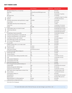


© Copyright 2026