
A Courseware Sample Instrumentation and Process Control 32621-F0
Instrumentation and Process Control
Courseware Sample
32621-F0
A
INSTRUMENTATION AND PROCESS CONTROL
COURSEWARE SAMPLE
by
the Staff
of
Lab-Volt Ltd.
Copyright © 2001 Lab-Volt Ltd.
All rights reserved. No part of this publication may be reproduced,
in any form or by any means, without the prior written permission
of Lab-Volt Ltd.
Printed in Canada
August 2007
Table of Contents
Introduction . . . . . . . . . . . . . . . . . . . . . . . . . . . . . . . . . . . . . . . . . . . . . . . . . . . V
Courseware Outline
Pressure, Flow, and Level Process Control . . . . . . . . . . . . . . . . . . . . . . . . VII
Temperature Process Control . . . . . . . . . . . . . . . . . . . . . . . . . . . . . . . . . . . XI
pH Process Control . . . . . . . . . . . . . . . . . . . . . . . . . . . . . . . . . . . . . . . . . . XIII
Sample Exercise Extracted from Pressure, Flow, and Level Process Control
Ex. 4-2
Differential-Pressure Level Meters . . . . . . . . . . . . . . . . . . . . . . . . . 3
Principle of operation of differential-pressure level meters. Measuring
the level of liquid in an open column with a differential-pressure
transmitter.
Sample Exercise Extracted from Temperature Process Control
Ex. 2-1
Resistance Temperature Detectors (RTDs) . . . . . . . . . . . . . . . . . 17
Construction and operation of RTDs. Comparison of the resistanceversus-temperature relationships of the most common types of RTDs.
Nominal resistance, temperature coefficient, and sensitivity.
Measurement of the voltage produced by an RTD with a Wheatstone
bridge.
Sample Exercise Extracted from pH Process Control
Ex. 2-1
pH Electrodes . . . . . . . . . . . . . . . . . . . . . . . . . . . . . . . . . . . . . . . . 39
An overview of the pH probe and of the pH Transmitter from the
Process Control Training System. Operation of the pH Transmitter in
both the fixed and the variable calibration modes. Measuring the pH
of different solutions using the pH Probe.
Other Sample Extracted from Pressure, Flow, and Level Process Control
Unit Test . . . . . . . . . . . . . . . . . . . . . . . . . . . . . . . . . . . . . . . . . . . . . . . . . . . 59
Instructor Guide Sample Extracted from Pressure, Flow, and Level Process
Control
Ex. 5-1
Pressure Process Control . . . . . . . . . . . . . . . . . . . . . . . . . . . . . . 63
Bibliography
III
IV
Introduction
The Lab-Volt Process Control Training System, Model 6090, familiarizes students
with the fundamentals of instrumentation and process control. It demonstrates the
control of pressure, flow, level, temperature, and pH processes. It can also
demonstrate advanced process control techniques, such as feed-forward control,
second-order control, and cascade control when used with a controller featuring
these functions.
The basic trainer demonstrates PID (proportional, integral, derivative) control of flow,
pressure, and level processes. It comes with a variable-speed pump, a tank, a
column, two-way valves, pressure gauges, flexible hoses, a venturi tube, an orifice
plate, a rotameter, a paddle wheel flow transmitter, and a differential pressure
transmitter. A work surface provides a large area on which components can be
mounted. Additional work area can be added with the provided expanding work
surface.
The trainer processes can be controlled by a computer-based PID Controller
implemented with a personal computer (Pentium type), the included Process Control
and Simulation Software (LVPROSIM), Model 3674, and the I/O Interface, Model
9065. The trainer processes can also be controlled using any conventional PID
controller compatible with standard 4-20 mA signals or 0-5 V signals.
To demonstrate PID control of temperature and pH processes, additional
components can be added to the basic trainer. The additional components required
for temperature process control include a heating unit, a cooling unit, and
temperature transmitters. Those required for pH process control include chemical
tanks, metering pumps, and a pH transmitter. Cascade and second-order process
control can also be studied with the basic trainer by having the students from two
workstations work together at a single workstation, or by adding the following
components to the basic trainer: a pressure transmitter, a column, and a PID
controller.
V
VI
Courseware Outline
PRESSURE, FLOW, AND LEVEL PROCESS CONTROL
Unit 1
Introduction to Process Control
Objective of process control. Open- and closed-loop process control.
Process Instrumentation. I.S.A. instrumentation symbols.
Ex. 1-1
Familiarization with the Training System
Introduction to the Process Control Training System.
Connection and operation of a basic flow circuit.
Unit 2
Pressure Processes
Nature of fluids. Definition and measurement of pressure. Pressure in a
water system.
Ex. 2-1
Pressure Measurement
Types of pressure measurement devices. Construction and
operation of liquid manometers, Bourdon-tube pressure
gauges, and strain-gauge pressure transmitters. Measuring
pressure with a pressure gauge, a pressure transmitter, and a
liquid manometer.
Ex. 2-2
Pressure Losses
Characteristics of fluids. Types of fluid flow. Reynolds number.
Definition of pressure loss. Factors affecting pressure loss.
Measuring the pressure losses in a water system.
Ex. 2-3
Centrifugal Pumps
Basic operation of a liquid pump. Types of liquid pumps.
Construction and operation of a centrifugal pump. Performance
chart, cavitation, NPSHR and NPSHA. Measuring the pressureversus-flow curve of a centrifugal pump at different rotation
speeds.
Ex. 2-4
Characterization of a Pressure Process
Dynamic characteristics of a process. Capacitance and
resistance of a process. Classification of processes.
Characterizing a pressure process by using the open-loop step
response method.
Unit 3
Flow Processes
Definition and measurement of flow rate. Types of devices used to
measure the flow rate of liquids.
VII
Courseware Outline
PRESSURE, FLOW, AND LEVEL PROCESS CONTROL (cont'd)
Ex. 3-1
Rotameters and Paddle Wheel Flow Meters
Construction and operation of rotameters and paddle wheel
flow meters. Plotting the voltage-versus-flow curve of a paddle
wheel flow transmitter.
Ex. 3-2
Orifice Plates
Bernouilli's principle. Introduction to differential-pressure flow
meters. Construction and operation of orifice plates. Beta ratio,
vena contracta, and permanent pressure loss. Plotting and
linearizing the pressure drop-versus-flow curve of an orifice
plate.
Ex. 3-3
Venturi Tubes
Construction and operation of venturi tubes. Throat, angle of
convergence, and angle of divergence. Plotting and linearizing
the pressure drop-versus-flow curve of a venturi tube.
Ex. 3-4
Permanent Pressure Losses Compared
Definition and measurement of power. Power conversion in a
water system. Power dissipated by a differential-pressure flow
meter. Calculation and comparison of the yearly electricity costs
of an orifice place and a venturi tube of equivalent size.
Ex. 3-5
Characterization of a Flow Process
Characterizing a flow process by using the open-loop step
response method.
Unit 4
Level Processes
Measurement of level. Point level and continuous level measurement
devices.
Ex. 4-1
Float Switches
Construction and operation of float switches. Float switch
applications. Using a float switch to limit the amount of liquid
pumped into a column.
Ex. 4-2
Differential-Pressure Level Meters
Principle of operation of differential-pressure level meters.
Measuring the level of liquid in an open column with a
differential-pressure transmitter.
VIII
Courseware Outline
PRESSURE, FLOW, AND LEVEL PROCESS CONTROL (cont'd)
Ex. 4-3
Zero Suppression and Zero Elevation
Calibrating a differential-pressure level meter so as to
compensate for the depression or elevation of its sensing
element relative to the reference level.
Ex. 4-4
Wet Reference Legs
Measuring the level of liquid in a pressurized column with a
differential-pressure level meter. Dry and wet reference legs.
Compensation of the hydrostatic pressure caused by a wet
reference leg.
Ex. 4-5
Characterization of a Level Process
Characterizing a level process by using the open-loop step
response method.
Ex. 4-6
Bubblers (Optional Exercise)
Principle of operation of bubblers. Measuring the level of liquid
in an open column by using a bubbler.
Unit 5
PID Process Control
Closed-loop control of a process. The PID controller. Types of
PID controller configurations. Tuning of a PID controller.
Ex. 5-1
Pressure Process Control
The trial and error method of controller tuning. Performing
PID control of a pressure process.
Ex. 5-2
Flow Process Control
The ultimate-cycle method of controller tuning. Performing
PID control of a flow process.
Ex. 5-3
Level Process Control
The open-loop step response method of controller tuning.
Performing PID control of a level process.
Ex. 5-4
Cascade Process Control
Comparison of the single-loop and cascade control modes.
Tuning of a cascade control system. Performing cascade
control of a level process.
IX
Courseware Outline
PRESSURE, FLOW, AND LEVEL PROCESS CONTROL (cont'd)
Ex. 5-5
Second-Order Process Control
Transfer function of a process. First- and second-order
processes. Characterization of a second-order process using
the open-loop step response method. Performing PID control of
a second-order level process.
Appendixes
A
B
C
D
Equipment Utilization Chart
Connection Diagrams
Detail of Pump Components
I.S.A. Instrumentation Symbols (Meaning of
the letter codes used in tag numbers)
E Selection Guide for Primary Sensing Elements
F Conversion Factors
G Using the Process Control and
Simulation Software (LVPROSIM)
Bibliography
We Value Your Opinion!
X
Courseware Outline
TEMPERATURE PROCESS CONTROL
Unit 1 Introduction to Temperature Process Control
Definition of thermal energy and temperature. Basic principles of thermal
energy (heat) transfer. Mechanisms of thermal energy transfer: conduction,
convection, and radiation.
Ex. 1-1 Familiarization with the Training System
The heating and cooling modes of control of temperature
processes. Familiarization with the components of the Process
Control Training System that are used for the measurement and
control of temperature.
Unit 2 Temperature Measurement
Temperature scales. Conversion between Celsius and Fahrenheit. Types
of temperature measurement devices commonly used in industrial
processes. Static and dynamic characteristics of temperature measurement
devices.
Ex. 2-1 Resistance Temperature Detectors (RTDs)
Construction and operation of RTDs. Comparison of the resistanceversus-temperature relationships of the most common types of
RTDs. Nominal resistance, temperature coefficient, and sensitivity.
Measurement of the voltage produced by an RTD with a
Wheatstone bridge.
Ex. 2-2 Thermocouples
The Seebeck effect. Construction and operation of thermocouples.
Comparison of the voltage-versus-temperature relationships of the
most common types of thermocouples. Cold junction compensation.
Thermocouple sensitivity to noise.
Ex. 2-3 Thermal Energy Transfer in Temperature Processes
Measurement of thermal energy. Specific heat capacity. Conversion
of energy in temperature processes. Thermal energy balance.
Determining the rate at which thermal energy is gained or lost by
water in a temperature process at thermal equilibrium.
Unit 3 Characterization of Temperature Processes
The Ziegler-Nichols and 28.3%-63.2% methods of process characterization.
XI
Courseware Outline
TEMPERATURE PROCESS CONTROL (cont'd)
Ex. 3-1 Characterization of a Temperature Process
in the Heating Mode
Characterizing a temperature process in the heating mode by using
the Ziegler-Nichols method of process characterization.
Ex. 3-2 Characterization of a Temperature Process
in the Cooling Mode
Characterizing a temperature process in the cooling mode by using
the 28.3%-63.2% method of process characterization.
Unit 4 PI Control of Temperature Processes
The control of temperature in the heating and cooling modes in a chemical
conversion process.
Ex. 4-1 PI Control of a Temperature Process in the
Heating Mode
Review of the principles of the ultimate-cycle method of PI controller
tuning. Performing PI control of a temperature process in the
heating mode.
Ex. 4-2 PI Control of a Temperature Process in the
Cooling Mode
Performing PI control of a temperature process in the cooling mode.
Calculation and tuning of the controller P and I constants, based on
the process characteristics measured in Exercise 3-2 with the
28.3%-63.2% method of process characterization.
Appendices A Equipment Utilization Chart
B Connection Diagrams
C I.S.A. Instrumentation Symbols (Meaning of
the letter codes used in tag numbers)
D Selection Guide for Temperature Sensing Elements
E Conversion Factors
F Using the Process Control and Simulation
Software (LVPROSIM)
Bibliography
We Value Your Opinion!
XII
Courseware Outline
pH PROCESS CONTROL
Unit 1 Introduction to pH Process Control
Concentration units. Definition of pH, acid solution, alkaline solution, and
buffer solution. Properties of acids and bases. Dissociation of acids and
bases. Analysis of titration curves.
Ex. 1-1
Familiarization with the Training System
Familiarization with the components of the Process Control
Training System that are used for the measurement and control
of pH. Introduction to the laboratory safety rules.
Unit 2 pH Measurement
Acids and bases characteristics. pH scale. Temperature effect on pH. Static
and dynamic characteristics of pH measurement devices. Mixing in pH
process reactors.
Ex. 2-1
pH Electrodes
An overview of the pH probe and of the pH Transmitter from the
Process Control Training System. Operation of the pH
Transmitter in both the fixed and the variable calibration modes.
Measuring the pH of different solutions using the pH Probe.
Ex. 2-2
Titration of a Strong Acid
Strong acids and strong bases. Calculation of the pH of a strong
acid solution and of a strong base solution . Titration of a strong
acid solution with a strong base solution. The effect of bad
mixing inside a reactor.
Ex. 2-3
Titration of Weak Acids
The 5% rule. Weak acids and weak bases. Calculation of the pH
of a weak acid solution and of a weak base solution. Titration of
weak acid solutions with a strong base.
Ex. 2-4
Titration of a Buffer Solution
Definition of buffer solution and buffer capacity. Using a sodium
bicarbonate solution as a buffer. Titration of a buffer solution with
a weak acid.
Unit 3 Characterization of pH Processes
Determining the dynamic characteristics of a process. The Ziegler-Nicholls,
28.3%-63.2%, and approximative method of process characterization.
XIII
Courseware Outline
pH PROCESS CONTROL (cont'd)
Ex. 3-1
Characterization of a Strong-Acid pH Process
Characterizing a strong-acid pH process using
Zeigler-Nichols method of process characterization.
Ex. 3-2
the
Characterization of a Weak-Acid pH Process
Characterizing a weak-acid pH process using the Zeigler-Nichols
method of process characterization.
Unit 4 pH Process Control
pH processes. Batch and continuous processes. Batch and continuous
processes examples.
Ex. 4-1
PID and On-Off Control of a Batch pH Process
On-off controller. On-off controller with a dead band. Performing
PID and on-off control of a batch pH process.
Ex. 4-2
PID Control of a Continuous pH Process
The open-loop step response method of controller tuning.
Performing PID control of a continuous pH process.
Appendices
A
B
C
D
E
F
G
H
Equipment Utilization Chart
Connection Diagrams
Physical Constants
Periodic Table of the Elements
Units Conversion Table
Calibrating the pH Transmitter
Useful Mathematical Formulas
Using the Process Control and Simulation Software
(LVPROSIM)
I
Neutralizing the system
J Rinsing the system
K Storage of the pH probe
L Material Safety Data Sheets
M Glossary
Bibliography
We Value Your Opinion!
XIV
Sample Exercise
Extracted from
Pressure, Flow, and
Level Process Control
Exercise
4-2
Differential-Pressure Level Meters
EXERCISE OBJECTIVES
C
C
C
To describe how differential-pressure level meters operate;
To describe the relationship between the hydrostatic pressure, density, and level
of liquid in a vessel;
To measure level in a column open to atmosphere by using a pressure
transmitter.
DISCUSSION
Measuring hydrostatic pressure in order to infer level
Unlike float switches, which allow detection of a single discrete level, differentialpressure level meters provide continuous measurement of the level of liquid in a
vessel.
Differential-pressure level meters do not measure the level directly. Instead they
measure a parameter that varies directly with the level of liquid in the vessel: the
hydrostatic pressure of the liquid. The hydrostatic pressure, also called hydraulic
head, is caused by the weight of the liquid in the vessel. The hydrostatic pressure
corresponds to the vertical height of the liquid column which would occur if the same
pressure was applied to the liquid.
The equation that relates the level of liquid in a vessel, h, to the hydrostatic pressure
of the liquid, Pg, is as follows:
S.I. system of units:
where
h
Pg
D
g
SG
=
=
=
=
=
level of the liquid (m);
hydrostatic pressure of the liquid (kPa, gauge);
mass density of the liquid (kg/m3);
gravitational acceleration (m/s2);
specific gravity of the liquid (dimensionless).
3
Differential-Pressure Level Meters
U.S. system of units:
where
*
h
Pg
gc
D
g
SG
=
=
=
=
=
=
level of the liquid (ft);
hydrostatic pressure of the liquid (psig);
dimensional constant (lbmAft/lbfAs2);
mass density of the liquid (lbm/ft3);
gravitational acceleration (ft/s2);
specific gravity of the liquid (dimensionless).
As previously mentioned, a pressure of 1 kPa corresponds to a column (head) of water of 0.102 m
at 15.5°C. Similarly, a pressure of 1 psi corresponds to a column of water of 2.31 ft at 60°F.
The equation shows that the level of the liquid varies in direct proportion to the
hydrostatic pressure of the liquid. This direct relationship is true provided that the
temperature and the density of the liquid remain constant in the vessel.
Note that the volume of the liquid also varies in direct proportion to the hydrostatic
pressure of the liquid, provided that the vessel is vertical and cylindrical in shape,
and that the temperature and the density of the liquid remain constant.
By measuring the hydrostatic pressure of a liquid with a pressure transmitter, we can
obtain a voltage or current proportional to the level of the liquid. This exercise will be
centered on the measurement of level in vessels that are open to atmosphere.
Measurement of the level in open vessels
In vessels that are open to atmosphere, the level is inferred by measuring the
hydrostatic gauge pressure of the liquid. To do this, either a gauge-pressure
transmitter or a differential-pressure transmitter can be used, as Figure 4-7 (a)
shows.
Note: The pressure transmitters of Figure 4-7 are represented by
the letters "LT" (standing for level transmitter) rather than by the
letters "PT" or "PDT". This occurs because flow diagrams represent
components according to their function, not their construction.
4
•
When a gauge-pressure transmitter (LT1) is used, the transmitter is connected
at the bottom of the vessel. The transmitter sensing line can contain the process
liquid, or it can contain a filling fluid that is removed from direct contact with the
process liquid by a seal.
•
When a differential-pressure transmitter (LT2) is used, the high-pressure side of
the transmitter is connected at the bottom of the vessel, while the low-pressure
side is left open to atmosphere.
Differential-Pressure Level Meters
Figure 4-7. Measurement of the level in a vessel that is open to atmosphere.
In either case, the voltage or current generated by the pressure transmitter will vary
in direct proportion to the level of the liquid in the vessel, as Figure 4-7 (b) shows.
This relationship is true provided that the temperature and the density of the liquid
remain constant in the vessel, which is normally the case.
The minimum measurable level is determined by where the primary sensing element
of the pressure transmitter is connected with respect to the bottom of the vessel. The
minimum level to be measured, or reference level, is adjusted by using the zero knob
of the transmitter, as Figure 4-7 (b) shows. The reference level can be set at the
minimum measurable level or above it.
The maximum measurable level is determined by the maximum height the liquid can
reach above the primary sensing element of the pressure transmitter. The maximum
level to be measured is adjusted by using the span knob of the transmitter, as
5
Differential-Pressure Level Meters
Figure 4-7 (b) shows. The maximum level to be measured can be set at the
maximum measurable level or below it.
Advantages and limitations
The measurement of liquid level through the measurement of hydrostatic pressure
is a method that is simple to apply, that requires minimum maintenance, and that
provides a good accuracy, generally in the order of ±1% of the actual span.
However, this method cannot be used with liquids that crystallize as their
concentration increases.
Moreover, a change in the temperature or density of the liquid dictates recalibration
of the transmitter. For example, heating the liquid will decrease the density of the
liquid and, therefore, will increase its volume. Consequently, the level of the liquid
will increase but the weight (and therefore the hydrostatic pressure) of the liquid will
remain the same, causing the pressure transmitter to indicate a level lower than the
actual level. Note, however, that some manufacturers offer "smart" transmitters that
can be programmed to compensate for the variation in liquid density.
Similarly, a change in the type of metered liquid dictates recalibration of the pressure
transmitter to account for the change in specific gravity (and therefore in density) of
the liquid. Figure 4-8, for example, shows the transmitter output-versus-level curves
obtained for three liquids of differing specific gravities when the pressure transmitter
is calibrated to accurately measure level at the specific gravity of water (1.00 at
15.5°C/60°F and normal atmospheric pressure). The transmitter indicates a level
higher than the actual level for the sulfuric acid and the chloroform. This occurs
because these denser (and therefore heavier) liquids produce a higher hydrostatic
pressure for any given level.
Figure 4-8. Pressure transmitter-versus-level curves obtained for three liquids of differing specific
gravities, when the transmitter is calibrated to accurately measure level at the specific gravity of
water (1.00).
6
Differential-Pressure Level Meters
Finally, in many installations, it is not possible to position the primary sensing
element of the pressure transmitter at exactly the same height as the desired
reference level. Thus, the sensing element may be located above or below the
reference level.
In those applications, the zero adjustment of the pressure transmitter must be
compensated to account for the elevation or depression of its sensing element with
respect to the desired reference level. You will learn more about this in the exercises
to follow.
Procedure summary
In this exercise, you will use a pressure transmitter to measure the level of the water
in a column that is open to atmosphere. You will plot the relationship between the
transmitter voltage and the level, demonstrating that the voltage varies linearly with
the level.
EQUIPMENT REQUIRED
Refer to the Equipment Utilization Chart in Appendix A of the manual to obtain the
list of equipment required to perform this exercise.
PROCEDURE
System setup
G
1. Get the Pressure Transmitter and Column from your storage location.
Mount these components on the Expanding Work Surface so that the
pressure ports of the Pressure Transmitter are approximately one row of
perforations above the bottom of the Column.
G
2. Set up the system shown in Figure 4-9. Make sure to connect the Rotameter
outlet to the port of the Column which is attached to a pipe that extends
down into column, which will reduce agitation of the water in the Column. On
the Column, make sure the cap of the insertion opening of the Float Switch
is tightened firmly.
Note: Level transmitter LT1 in Figure 4-9 is actually a pressure
transmitter. This occurs because flow diagrams represent
components according to their function, not their construction.
Note: The Column will first be operated in the pressurized mode
in order to purge air from the hose connecting the bottom of the
Column to the Pumping Unit. Failure to purge air from this hose
can prevent the water in the Column from decreasing below a
certain level when the pump speed is decreased or the pump is
stopped.
7
Differential-Pressure Level Meters
Figure 4-9. Measuring the water level in an open column by using a Pressure Transmitter.
G
3. Power up the Pressure Transmitter.
G
4. Make the following settings on the Pressure Transmitter:
ZERO adjustment knob . . . . . . . . . . . . . . . . . . . . . . . . . . . . . . . MAX.
SPAN adjustment knob . . . . . . . . . . . . . . . . . . . . . . . . . . . . . . . MAX.
LOW PASS FILTER switch . . . . . . . . . . . . . . . . . . . . . . . . . . . . I (ON)
G
5. Make sure the reservoir of the Pumping Unit is filled with about 12 liters
(3.2 gallons US) of water. Make sure the baffle plate is properly installed at
the bottom of the reservoir.
G
6. On the Pumping Unit, adjust valves HV1 to HV3 as follows:
–
–
–
8
Open HV1 completely;
Close HV2 completely;
Set HV3 for directing the full reservoir flow to the pump inlet.
Differential-Pressure Level Meters
G
7. Turn on the Pumping Unit.
G
8. With the controller in the manual (open-loop) mode, set the controller output
at 100%, which will cause the water level to rise in the Column.
G
9. Close valve HV1 of the Pumping Unit completely, which will cause the water
level to rise further in the Column.
G 10. Set the controller output at 0% to stop the Pumping Unit. This will cause part
of the water in the Column to siphon back out the tube in the Column.
G 11. Remove the plug connected to the hose port at the top of the Column.
Connect this port to either of the auxiliary return ports of the Pumping Unit,
using an extra-long hose.
This hose will serve as an overflow if the Column gets full. Moreover, it will
cause the Column to be open to atmosphere through the reservoir of the
Pumping Unit.
G 12. Set the controller output at 50% to make the water level rise into the
Column. Then open valve HV1 of the Pumping Unit completely.
Transmitter calibration
Note: In steps 13 through 17, you will be adjusting the ZERO and
SPAN knobs of the Pressure Transmitter so that its output voltage
varies between 0.00 and 5.0 V DC when the level of the water in
the Column is varied between 5 and 56 cm (2 and 22 in).
G 13. Connect a DC voltmeter to the 0-5 V OUTPUT of the Pressure Transmitter.
G 14. Adjust the controller output until the water level is stable at 5 cm (2 in) in the
Column. This will be the reference level.
Note: From now on, it is important that the water level in the
Column not be allowed to fall below 4 cm (1.5 in), as this would
cause air to enter the line between the bottom of the Column and
the Pumping Unit, which in turn would prevent the water in the
Column from dropping below a certain level when the pump
speed is reduced or the pump is stopped. Should this situation
occur, you will have to purge air from this line by placing the
Column in the pressurized mode as shown in Figure 4-9 and then
repeating procedure steps 4 through 12.
9
Differential-Pressure Level Meters
G 15. While observing the DC voltmeter reading, turn the ZERO adjustment knob
of the Pressure Transmitter counterclockwise to decrease the voltage and
stop turning it as soon as the voltmeter reads 0.00 V.
G 16. Readjust the controller output to raise and stabilize the water level to 56 cm
(22 in) in the Column.
G 17. Adjust the SPAN knob of the Pressure Transmitter until the DC voltmeter
reads 5.0 V.
Note: Due to interaction between the ZERO and SPAN
adjustments of the Pressure Transmitter, it will be necessary to
repeat steps 14 through 17 until the Pressure Transmitter output
voltage actually varies between 0.00 and 5.0 V DC when the level
of the water is varied between 5 and 56 cm (2 and 22 in).
Determining the relationship between the level and the pressure transmitter
voltage
G 18. By varying the controller output, raise the water level in the Column from 5
to 55 cm by steps of 5 cm (or from 2 to 22 in by steps of 2 in).
After each new level setting, measure the voltage generated by the
Pressure Transmitter and record it in Table 4-1.
LEVEL [cm (in)]
PRESSURE TRANSMITTER
VOLTAGE (V)
5 cm (2 in)
0.00 V
Table 4-1. Voltage generated by the Pressure Transmitter as a function of the water level in the
open Column.
10
Differential-Pressure Level Meters
G 19. Stop the variable-speed drive of the Pumping Unit by setting the controller
output at 0%.
G 20. From the data recorded in Table 4-1, plot in Figure 4-10 the relationship
between the water level and the Pressure Transmitter voltage.
G 21. According to the curve obtained in Figure 4-10, does the voltage generated
by the Pressure Transmitter increase linearly as the level is increased?
Why?
G 22. If the water in the Column was replaced by mercury without recalibrating the
Pressure Transmitter, would the transmitter indicate higher or lower than the
actual liquid level? Explain.
11
Differential-Pressure Level Meters
Figure 4-10. Relationship between the water level and the Pressure Transmitter voltage.
G 23. Turn off the Pumping Unit by setting its POWER switch at O.
G 24. Disconnect the circuit. Return the components and hoses to their storage
location.
12
Differential-Pressure Level Meters
G 25. Wipe off any water from the floor and the Process Control Training System.
CONCLUSION
In this exercise, you measured the voltage produced by a pressure transmitter as a
function of the water level in an open column. This allowed you to see that the
hydrostatic gauge pressure of the water in the column varies in direct proportion to
the water level in the column. This direct relationship is true, provided that the
density and the temperature of the water remain constant.
REVIEW QUESTIONS
1. How does the level of the liquid in an open vessel vary with the hydrostatic
gauge pressure of the liquid in the vessel, for any given density and
temperature?
2. What effect does increasing the temperature of the liquid in a vessel have on the
density and level of the liquid?
3. What is the level of the water in an open vessel if the hydrostatic pressure of the
water is 100 kPa, gauge (14.5 psig) at 15.5°C (60°F)?
4. If the liquid in a vessel was changed for a liquid of lower specific gravity than that
at which the pressure transmitter was calibrated, would the transmitter read
higher or lower than the actual liquid level? Explain.
13
Differential-Pressure Level Meters
5. How could a pressure transmitter calibrated to accurately read level at a specific
gravity of 1.00 be used to measure the level of a liquid with a specific gravity of
2.00?
14
Sample Exercise
Extracted from
Temperature Process Control
Exercise
2-1
Resistance Temperature Detectors (RTDs)
EXERCISE OBJECTIVES
•
•
•
•
To explain how resistance temperature detectors (RTDs) operate;
To describe the relationship between the temperature and the electrical
resistance of the most common types of RTDs;
To define the following terms: nominal resistance, temperature coefficient, and
sensitivity.
To explain how a Wheastone bridge can be used to measure the voltage
produced across an RTD.
DISCUSSION
Electrical resistance
An important characteristic of all metals is their electrical resistance. Electrical
resistance is the opposition of the metal to the flow of electrical current. Electrical
resistance is measured in ohms (S) in both the S.I. and U.S. systems of units.
The electrical resistance of a metal is dependent upon the temperature at which the
metal is. Figure 2-4, for example, shows what happens to the relative resistance of
different metals as their temperature increases. The relative resistance is the ratio
between the resistance at the applied temperature to the resistance at a reference
temperature of 0°C (32°F).
As the figure shows, the relative resistance of the metals increases as their
temperature gets higher. Moreover, the relative resistance increases almost linearly
with temperature, at least over a substantial range of temperatures. Besides, the
relative resistance of nickel increases more sharply with temperature than that of
copper or platinum.
17
Resistance Temperature Detectors (RTDs)
Figure 2-4. Relative resistance-versus-temperature relationship of different metals.
Temperature coefficient
All metals have a specific temperature coefficient that indicates their average
change in relative resistance per unit of temperature between 0 and 100°C (between
32 and 212°F).
The temperature coefficient is symbolized by the Greek letter alpha ("). It is usually
measured in ohms per ohm degree Celsius (°C-1) or in ohms per ohm degree Fahrenheit (°F-1).
Figure 2-4, for example, indicates that the temperature coefficient of platinum is
0.00392°C-1 (0.00218°F-1). Consequently, the relative resistance of platinum varies
by 0.392 between 0 and 100°C (32 and 212°F). Beyond 100°C (212°F), the shape
of the platinum curve indicates that the temperature coefficient decreases slightly as
the temperature gets higher.
18
Resistance Temperature Detectors (RTDs)
Resistance temperature detectors
A resistance temperature detector (RTD) is a primary element that is used to sense
temperature. The RTD works on the principle that the electrical resistance of metals
changes with temperature.
The RTD consists of a metallic conductor usually wound into a coil. The RTD is to
be connected to an electrical circuit in order to make a constant excitation current
flow through it. As the temperature increases, the electrical resistance of the metallic
conductor increases and, therefore, the voltage across the RTD increases.
Consequently, by measuring the voltage across the RTD, a signal proportional to the
temperature of the RTD can be obtained. This signal can be conditioned into a
current, voltage, or pressure of normalized range that is suitable for instrumentation
and control, the combination of the RTD and the conditioning circuit thus forming a
temperature transmitter.
RTD metals
The selection of a metal for use as an RTD depends on several factors. Among
these, the most important are the capability to follow rapidly changing temperatures,
a good linearity, a good reproducibility, and a relatively high change of resistance for
a given change in temperature (i.e. a high temperature coefficient).
The metals most commonly used for RTDs are platinum, nickel, and copper (refer
to Figure 2-4):
•
Platinum is the preferred metal for RTDs. It has been chosen as the
international standard metal for RTD temperature measurement. Platinum has
a nearly linear resistance-versus-temperature relationship over a wide
temperature range. Platinum offers good stability and reproducibility. It is wellsuited for the measurement of high temperatures up to 650°C (1200°F).
•
Nickel is the second mostly used metal for RTDs. It is less expensive than
platinum and it is more sensitive because of its higher temperature coefficient.
However, nickel has a narrower sensing range than platinum and is limited to the
measurement of temperatures below 300°C (570°F).
•
Copper is the least expensive of the three metals and it has the most linear
relationship. Similar to platinum, copper is well suited for the measurement of
high temperatures. However, copper is subject to oxidation, and it has poorer
stability and reproducibility than platinum.
RTD characteristics
Two important characteristics of RTDs are their nominal resistance and their
temperature coefficient:
•
The nominal resistance is the resistance of the RTD at a given reference
temperature, as specified by the manufacturer. Platinum RTDs, for example, are
usually designed so that their nominal resistance is 100 S at the ice reference
point of 0°C (32°F).
19
Resistance Temperature Detectors (RTDs)
•
The temperature coefficient is the mean change in relative resistance of the
metal per unit of temperature between 0 and 100°C (32 and 212°F), as
previously explained.
The nominal resistance and the temperature coefficient of an RTD determine the
sensitivity of the RTD within the 0-100°C (32-212°F) temperature range. The
sensitivity is the amount by which the resistance of the RTD will change per unit of
temperature, in S/°C (or S/°F).
For example, a platinum RTD having a nominal resistance of 100 S at 0°C (32°F)
and a temperature coefficient of 0.00392°C-1 (0.00218°F-1) will have a sensitivity of
0.392 S/°C (0.218 S/°F) within the 0-100°C (32-212°F) temperature range.
Measurement of the voltage across an RTD
As previously mentioned, the voltage produced across an RTD, which is directly
proportional to temperature, can be used for process instrumentation and control.
The traditional method of measuring the voltage across an RTD is to use a
Wheatstone bridge, as Figure 2-5 (a) shows.
•
The RTD and its two lead wires constitute one leg of the bridge. Resistors R1 and
R2 are of equal resistance, while resistor R3 is adjustable and is used as a
reference.
•
A DC voltage source supplies an excitation current to the RTD.
•
A differential amplifier produces a voltage VO proportional to the bridge output
voltage (measured between points a and b).
With the RTD placed in an ice bath at 0°C (32°F), resistor R3 is initially adjusted in
order to obtain a null voltage (0 V) at the output of the differential amplifier. In this
condition, the bridge is said to be null balanced.
Once the bridge has been null balanced, the amplifier output voltage will vary in
direct proportion to the temperature of the RTD.
20
Resistance Temperature Detectors (RTDs)
Figure 2-5. Measurement of the voltage across an RTD.
If the two leads that connect the RTD to the bridge are more than a few centimeters
(inches) long, they will introduce an error in the temperature measurement. This
occurs because the resistance of the leads will contribute to the voltage produced
at the output of the bridge, causing the measured temperature to be higher than that
actually measured.
To minimize this error, RTDs are available in a three-wire version. The extra wire is
used to cancel the resistances of lead wires 1 and 2 by balancing the bridge, as
Figure 2-5 (b) shows. This has the effect of removing the error produced by lead
wires 1 and 2 as long as these wires are of equal resistance (i.e. of equal length and
temperature).
Advantages and limitations of RTDs
RTDs have the following advantages: they provide a good sensitivity, a good
reproducibility, and a good stability. They also provide a high accuracy, some
platinum RTDs being able to measure a few thousandths of a degree.
However, RTDs are relatively expensive, and they have a slower response time than
thermocouples. Moreover, the measurement accuracy of RTDs is dependent upon
the thermal stability of the resistors and power supply used in the Wheatstone
bridge.
The RTD probe and the RTD Temperature Transmitter of the Process Control
Training System
The Process Control Training System comes with a three-wire RTD probe that uses
a platinum RTD of 100 S at 0°C (32°F). The RTD probe is intended to be used with
the RTD Temperature Transmitter to measure the temperature of the water in the
trainer Column, as Figure 2-6 shows.
21
Resistance Temperature Detectors (RTDs)
The tip of the RTD probe, which contains the RTD, is to be inserted into the Column
through the opening of the Float Switch. The other end of the RTD probe, which has
three leads, is to be connected to the "100-S RTD" terminals of the RTD
Temperature Transmitter.
The RTD Temperature Transmitter produces an excitation current through the RTD
and it measures the resulting voltage produced across the RTD. This voltage, which
is proportional to the temperature of the RTD, is conditioned into normalized voltages
and current that are available at the transmitter OUTPUTS.
The transmitter also contains a calibration source that can be used to simulate the
voltage produced across the RTD for any RTD temperature comprised between 0
and 100°C (32 and 212°F). The source eliminates the need to set the RTD at a wellknown temperature when performing calibration of the transmitter OUTPUTS.
The following is a detailed description of the RTD Temperature Transmitter terminals
and adjustments (refer to Figure 2-6):
Î
POWER INPUT terminals: used to power the transmitter with a DC voltage
of 24 V.
Ï
CALIBRATION SOURCE adjustment knob: sets the probe temperature to
be simulated by the calibration source signal. This temperature can be
adjusted between 0 and 100°C (32 and 212°F).
Ð
INPUT SELECTOR: selects between the actual probe signal or the
simulated probe signal produced by the calibration source.
Ñ
CALIBRATION SELECTOR switch: places the 0-5 V and 4-20 mA
OUTPUTS in either fixed or variable calibration mode.
Ò
ZERO and SPAN adjustment knobs: used in the variable calibration mode
(CALIBRATION SELECTOR switch at VARIABLE) to set the temperature
range for which the 0-5 V and 4-20 mA OUTPUTS will pass from minimum
to maximum:
– The ZERO knob sets the temperature for which the outputs will be
minimum (0 V and 4 mA), i.e. the minimum temperature to be
detected. The minimum temperature can be adjusted between 0 and
50°C (32 and 122°F).
– The SPAN knob sets the temperature for which the outputs will be
maximum (5 V and 20 mA), i.e. the maximum temperature to be
detected. The maximum temperature can be adjusted between 15
and 30°C (27 and 54°F) above the minimum temperature set by the
ZERO knob.
22
Resistance Temperature Detectors (RTDs)
Figure 2-6. The RTD probe and RTD Temperature Transmitter of the Training System.
Ó
CALibrated OUTPUT: provides a voltage proportional to the temperature
sensed by the probe or to the simulated probe signal produced by the
calibration source, depending on the position of the INPUT SELECTOR
switch.
23
Resistance Temperature Detectors (RTDs)
This output has a fixed calibration of 100 mV per sensed °C above 0°C
(or 56 mV per sensed °F above 32°F). It will pass from 0 to 10 V when
the actual or simulated temperature changes from 0 to 100°C (32 to
212°F).
Ô
0-5 V and 4-20 mA OUTPUTS terminals: provide a voltage and a current
proportional to the temperature sensed by the probe or to the probe
temperature signal simulated by the calibration source, depending on the
position of the INPUT SELECTOR switch.
The calibration of the 0-5 V and 4-20 mA OUTPUTS can be either fixed
or variable, depending on the position of the CALIBRATION
SELECTOR switch:
– In the fixed calibration mode (CALIBRATION SELECTOR switch at
FIXED), the temperature range for which the outputs will pass from
minimum to maximum is fixed and is 0-100°C (32-212°F).
– In the variable calibration mode (CALIBRATION SELECTOR switch
at VARIABLE), the temperature range for which the outputs will pass
from minimum to maximum can be adjusted by means of the ZERO
and SPAN adjustment knobs.
Õ
100-S RTD input terminals: used to connect the RTD probe to the
transmitter.
Procedure summary
In the first part of the exercise, you will familiarize yourself with the operation of an
RTD Temperature Transmitter in the fixed calibration mode.
In the first part of the exercise, you will familiarize yourself with the operation of an
RTD Temperature Transmitter in the variable calibration mode.
In the third part of the exercise, you will set up and operate a temperature process.
You will use an RTD Temperature Transmitter to measure the temperature of the
water in a column.
EQUIPMENT REQUIRED
Refer to the Equipment Utilization Chart in Appendix A of the manual to obtain the
list of equipment required to perform this exercise.
24
Resistance Temperature Detectors (RTDs)
PROCEDURE
Operation of the RTD Temperature Transmitter in the fixed calibration mode
G
1. Get the RTD Temperature Transmitter and 24-V DC Power Supply from
your storage area. Mount these components on the Main Work Surface.
G
2. Power up the RTD Temperature Transmitter.
G
3. Get the RTD probe from your storage location and connect it to the
100-S RTD input of the RTD Temperature Transmitter.
Let the probe tip lie on the Work Surface.
G
4. Make the following settings on the RTD Temperature Transmitter:
INPUT SELECTOR . . . . . . . . . . . . . . . . . . . . . . . . . . . . . . . . . . . RTD
CALIBRATION SELECTOR . . . . . . . . . . . . . . . . . . . . . . . . . . FIXED
This selects the RTD probe signal as the transmitter input signal and places
the transmitter OUTPUTS in the fixed calibration mode.
G
5. Connect a DC voltmeter to the 0-5 V OUTPUT of the RTD Temperature
Transmitter.
Since this output is in the fixed calibration mode, it generates a fixed voltage
of 50 mV per sensed °C above 0°C (or 28 mV per sensed °F above 32°F).
According to the voltmeter reading, what is the ambient temperature?
G
6. Further experiment with the operation of the transmitter in the fixed
calibration mode:
–
Fill a suitable container with ice water (a mixture of ice cubes and
water).
–
Immerse the tip of the RTD probe into the ice water. The 0-5 V
OUTPUT voltage should decrease and stabilize at about 0.0 V, which,
in the fixed calibration mode, corresponds to an RTD temperature of
0°C (32°F).
–
Fill a suitable container with boiling water heated by an electric kettle or
a microwave oven.
–
Immerse the tip of the RTD probe into the boiling water. The 0-5 V
OUTPUT voltage should increase and stabilize at about 5.0 V, which,
25
Resistance Temperature Detectors (RTDs)
in the fixed calibration mode, corresponds to an RTD temperature of
100°C (212°F).
Note: The 0-5 V OUTPUT of the RTD Temperature Transmitter
will stabilize at a voltage lower than 5.0 V if the atmospheric
pressure is lower than 101.3 kPa, absolute (14.7 psia).
Record below your observations.
Operation of the RTD Temperature Transmitter in the variable calibration mode
Note: In the following steps, you will use the calibration source
of the RTD Temperature Transmitter to calibrate its 0-5 V
OUTPUT so that the voltage at this output passes from 0.0 to
5.00 V when the probe temperature simulated by the calibration
source passes from 25 to 55°C (77 to 131°F), respectively.
G
7. Make the following settings on the RTD Temperature Transmitter:
INPUT SELECTOR . . . . . . . . . . . . . . . . . . . . . . . . . . CAL. SOURCE
CALIBRATION SELECTOR . . . . . . . . . . . . . . . . . . . . . . . VARIABLE
ZERO adjustment knob . . . . . . . . . . . . . . . . . . . . . . . . . . . . . . . MAX.
SPAN adjustment knob . . . . . . . . . . . . . . . . . . . . . . . . . . . . . . . MAX.
This selects the calibration source signal as the transmitter input signal and
places the transmitter OUTPUTS in the variable calibration mode.
G
8. Set the probe temperature to be simulated by the calibration source of the
transmitter at 25°C (77°F).
To do so, adjust the CALIBRATION SOURCE knob of the transmitter until
you obtain a voltage of 2.5 V at the CAL. OUTPUT of the transmitter.
G
9. While monitoring the voltage at the 0-5 V OUTPUT of the transmitter, turn
the ZERO adjustment knob counterclockwise and stop turning it as soon as
the voltage ceases to decrease, which should occur around 0.01 V. Then
very slowly turn the knob in the clockwise direction and stop turning it as
soon as the voltage starts to increase.
This sets the minimum temperature to be detected at 25°C (77°F)
approximately.
G 10. Now set the probe temperature to be simulated by the calibration source of
the transmitter at 55°C (131°F).
To do so, adjust the CALIBRATION SOURCE knob of the transmitter until
you obtain a voltage of 5.5 V at the CAL. OUTPUT of the transmitter.
26
Resistance Temperature Detectors (RTDs)
G 11. Adjust the SPAN knob in order to obtain a voltage of 5.00 V at the
transmitter 0-5 V OUTPUT.
This sets the maximum temperature to be detected at 55°C (131°F)
approximately.
G 12. Now that the RTD Temperature Transmitter is calibrated, proceed to the
next part of the exercise.
Measuring temperature with an RTD
Preliminary setup
G 13. Get the Expanding Work Surface from your storage location and mount it
vertically (at an angle of 90°) to the Main Work Surface, if this has not
already been done.
G 14. Connect the system shown in Figure 2-7, being careful not to modify the
calibration settings just made on the RTD Temperature Transmitter.
Figure 2-8 shows the suggested setup.
The speed of the variable-speed drive of the Pumping Unit will be controlled
with a controller, FIC1, placed in the manual (open-loop) mode. The Heating
and Cooling Units will be controlled manually. (This is the reason why there
is no temperature controller, or "TC" instrumentation symbol illustrated next
to these units in the flow diagram of Figure 2-7.)
The Column will first be operated in the pressurized mode in order to purge
air from the components downstream of the Column. Consequently, let the
tip of the RTD probe lie on the Work Surface for now.
Note: Make sure to mount the Heating Unit at the highest
possible location on the Expanding Work Surface, in order for this
unit to be above the other process components, as Figure 2-8
shows. Failure to do so may result in water entering the Heating
Unit upon disconnection of the hoses, which in turn might cause
damage to the Heating Unit.
Moreover, mount the 24-V DC Power Supply and the RTD
Temperature Transmitter in such a manner that water cannot
enter these components and their electrical terminals when hoses
are disconnected.
The Heating Unit must be connected for the direction of flow
indicated by the arrow heads in the symbol on its front panel.
27
Resistance Temperature Detectors (RTDs)
On the other hand, the Cooling Unit will operate regardless of the
direction of water flow through it. However, to minimize the risk of
cavitation caused by air suction within the pump when the water
becomes hot, connect the Cooling Unit as indicated in Figure 2-8,
that is, with the upper unit port used as the hot water inlet and the
lower unit port used as the cooled water outlet. For the same
reason, mount the Column at the highest possible location on the
Expanding Work Surface in order to create a substantial head of
water upstream of the Cooling Unit.
Note: If the controller you are using as flow controller FIC1 is the
Lab-Volt Process Control and Simulation Software (LVPROSIM),
model 3674, you can refer to Figure B-1 of Appendix B for details
of how to connect the LVPROSIM computer to the variable-speed
drive (SC1) of the Pumping Unit.
Figure 2-7. Measuring temperature with an RTD temperature transmitter.
28
Resistance Temperature Detectors (RTDs)
Figure 2-8. Suggested setup for the diagram of Figure 2-7 (see table next page for the detail of the
components).
29
Resistance Temperature Detectors (RTDs)
Î : Column
Ò : Cooling Unit
Ï : Heating Unit
Ó : RTD probe
Ð : Paddle Wheel Flow Transmitter
Ô : RTD Temperature Transmitter
Ñ : Pumping Unit
Õ : DC Power Supply
G 15. Make the following settings:
On the Heating Unit:
S1 switch . . . . . . . . . . . . . . . . . . . . . . . . . . . . . . . . . . . . . . . . . . 2
Manual control knob . . . . . . . . . . . . turned fully counterclockwise
On the Cooling Unit:
S1 switch . . . . . . . . . . . . . . . . . . . . . . . . . . . . . . . . . . . . . . . . . . 2
Manual control knob . . . . . . . . . . . . turned fully counterclockwise
S2 switch . . . . . . . . . . . . . . . . . . . . . . . . . . . . . . . . . . . . . . . . . .
On the RTD Temperature Transmitter:
SELECTOR switch . . . . . . . . . . . . . . . . . . . . . . . . . . . . . . . . RTD
Note: The 0-5 V OUTPUT of the RTD Temperature Transmitter
should still be calibrated for a temperature measurement range of
25-55°C (77-131°F) from the first part of the exercise.
G 16. Power up the Heating Unit:
–
–
Connect the AC line cord of this unit to a wall outlet.
Set the POWER switch at I.
G 17. Power up the Cooling Unit and the Paddle Wheel Flow Transmitter by
connecting their POWER INPUT terminals to the 24-V DC Power Supply.
Purging air from the components downstream of the Column
G 18. Make sure flow controller FIC1 is in the manual (open-loop) mode. Set the
output of this controller at 0% (0 V).
G 19. On the Column, make sure the cap of the insertion opening of the Float
Switch is tightened firmly.
30
Resistance Temperature Detectors (RTDs)
G 20. Make sure the reservoir of the Pumping Unit is filled with about 12 liters
(3.2 gallons US) of water. Make sure the baffle plate is properly installed at
the bottom of the reservoir.
G 21. Turn on the Pumping Unit by setting its POWER switch at I.
G 22. On the Pumping Unit, adjust valves HV1 through HV3 as follows:
–
–
–
Open HV1 completely;
Close HV2 completely;
Set HV3 for directing the full reservoir flow to the pump inlet (turn handle
fully clockwise).
G 23. Make the variable-speed drive of the Pumping Unit rotate at the maximum
speed: with controller FIC1 in the manual (open-loop) mode, set the
controller output at 100% (5 V).
G 24. Allow the level of the water to rise in the pressurized Column until it
stabilizes at some intermediate level. This will force air out of the
components downstream of the Column.
Note: If the cap of the insertion opening of the Float Switch on
the Column has not been tightened firmly, air will be allowed to
escape from the Column and the water level will not stabilize in
the Column. Should this case occur, stop the variable-speed drive
of the Pumping Unit. Open valves HV1 and HV2 of the Pumping
Unit in order to drain the Column to the reservoir. When the
Column is empty, tighten the cap of the insertion opening of the
Float Switch on the Column with more force. Then resume the
procedure from step 22.
Placing the system in the water recirculating mode
Note: In the following steps, you will place the system in the
water recirculating mode by setting the Pumping Unit valves so as
to direct the return flow directly to the pump inlet, not to the
reservoir. This will reduce the time required to raise or decrease
the temperature of the process water. For the same reason, the
water level in the Column will be set at a low, minimum level of
7.5 cm (3 in).
G 25. On the Pumping Unit, close valve HV1, which will cause the water level to
rise further in the Column. Then set valve HV3 for directing the full return
flow directly to the pump inlet (turn handle fully counterclockwise).
G 26. On the Column, remove the cap of the insertion opening of the Float Switch
to depressurize the Column. (The water level in the Column will remain
stable).
31
Resistance Temperature Detectors (RTDs)
G 27. On the Pumping Unit, open valve HV2 in order to decrease the water level
in the Column to 7.5 cm (3 in), then close this valve.
G 28. Readjust the output of controller FIC1 until you read 4.0 V approximately at
the "F (cal.)" output of the Paddle Wheel Flow Transmitter. This will set the
flow rate at about 4 l/min (1.1 gal US/min).
Note: Small, continuous variations of a few tenths of volts around
the adjusted mean value of 4.0 V are normal at the flow
transmitter output.
However, large variations of one volt or more are abnormal, and
indicate that air has entered the system through an untight
connector or component on the suction side of the pump.
Should that case occur, stop the variable-speed drive of the
Pumping Unit in order to drain the column to the reservoir. When
the Column is empty, check the inside of the connector on the
Pumping Unit return line hose for any dirt or particles. Also, check
the o-rings on the two hose connectors of the Cooling Unit for any
fissure or crack. Once you have located and eliminated the cause
of the leak, reconnect the system as in Figure 2-7 and resume the
procedure from step 19.
Measuring temperature with the RTD
G 29. Insert the RTD probe all the way into the Column in order for its tip to be
submerged in the water.
G 30. Have the signal at the 0-5 V OUTPUT of the RTD Temperature Transmitter
plotted on the trend recorder of controller FIC1.
Adjust the update rate of the trend recorder (sampling interval) in order to
be able to monitor the transmitter signal over a period of 10 minutes
approximately.
Note: If the controller you are using as controller FIC1 is the LabVolt Process Control and Simulation Software (LVPROSIM),
model 3674, refer to Figure B-5 of Appendix B for details of how
to connect the LVPROSIM computer to the RTD Temperature
Transmitter. On the I/O Interface, make sure the RANGE switch
of ANALOG INPUT 1 is set at 5 V.
In LVPROSIM, select Analog Input 1 from the Trend Recorder
selection list to have the RTD Temperature Transmitter signal
plotted on the trend recorder. Set the LVPROSIM sampling
interval at 1500 ms. Access the Configure Analog Inputs window
and set the minimum and maximum range values of Analog
Input 1 at 25 and 55°C (77 and 131°F), respectively, which
corresponds to the current measurement range of the RTD
Temperature Transmitter. Set the filter time constant of this input
at 0.5 second. Make sure the square root extracting function is
unselected. Accept setup and return to main screen.
32
Resistance Temperature Detectors (RTDs)
G 31. On the trend recorder, observe the RTD Temperature Transmitter output
signal.
Since no electrical power is applied to the heating element of the Heating
Unit, theoretically, the water in the Column should be at ambient
temperature.
Assuming that the ambient temperature is below 25°C (77°F), the level of
the RTD Temperature Transmitter signal should be at 0% of span on the
trend recorder, since the minimum temperature the transmitter can detect
has been adjusted to 25°C (77°F).
Yet, you may observe that the RTD Temperature Transmitter signal is at
some higher level, thermal energy being transferred to the recirculated
water mainly from frictional resistance of the pump internal parts.
G 32. On the Heating Unit, set the manual control knob to the mid position. On the
trend recorder, observe what happens to the temperature of the water in the
Column.
Now that electrical power is applied to the heating element of the Heating
Unit, thermal energy is transferred from this element to the recirculated
water.
Consequently, the temperature of the water should increase in the Column.
Is this your observation?
G Yes
G No
G 33. Let the temperature of the water in the Column increase to about 45°C
(113°F), or 67% of span, then turn the manual control knob of the Heating
Unit fully counterclockwise to remove electrical power from its heating
element.
According to the RTD Temperature Transmitter output signal on the trend
recorder, did the temperature of the water in the Column increase linearly
over time?
How long did it take for the temperature to increase from the initial
temperature to the final temperature of 45°C (113°F)?
33
Resistance Temperature Detectors (RTDs)
G 34. On the Cooling Unit, turn the manual control knob fully counterclockwise.
What happens to the temperature of the water in the Column?
G 35. Allow the temperature of the water in the Column to cool down.
According to the RTD Temperature Transmitter output signal, does the
temperature of the water in the Column decrease linearly over time?
Explain.
G 36. Stop the variable-speed drive of the Pumping Unit by setting the output of
controller FIC1 at 0%.
G 37. Turn off the Pumping Unit, the Heating Unit, and the 24-V DC Power Supply
by setting their POWER switch at O.
G 38. Open valve HV1 of the Pumping Unit completely and let the water in the
Column drain back to the reservoir. The Column can also be drained by
disconnecting the end of the hose connected to the Cooling Unit inlet port
and reconnecting it to either of the auxiliary return ports on the Pumping
Unit.
G 39. Disconnect the system. Return all leads, hoses, and components to their
storage location.
CAUTION!
Hot water may remain in the hoses and components. Be
careful not to allow water to enter the electrical components
and their terminals upon disconnection of the hoses.
G 40. Wipe off any water from the floor and the Process Control Training System.
CONCLUSION
In this exercise, you familiarized yourself with the operation of an RTD temperature
transmitter in the fixed and variable calibration modes. You learned that, in the fixed
calibration mode, the temperature measurement range is fixed and is equal to 0100°C (32-212°F). In the variable calibration mode, the temperature measurement
range can be adjusted, and a maximum span of 30°C (54°F) can be obtained. Since
this span is narrower than the 100°C (180°F) span of the fixed calibration mode, the
variable calibration mode provides a greater measurement accuracy for any given
transmitter output range.
34
Resistance Temperature Detectors (RTDs)
REVIEW QUESTIONS
1. What is an RTD? How does an RTD work?
2. What are three metals commonly used for RTDs? What are the advantages and
limitations of each metal?
3. Name and describe two important characteristics of RTDs.
4. How is the voltage produced across an RTD traditionally measured?
5. Why are RTDs available in three-wire version? Explain.
35
36
Sample Exercise
Extracted from
pH Process Control
Exercise
2-1
pH Electrodes
EXERCISE OBJECTIVES
•
•
•
•
To explain how pH electrodes operate;
To familiarize yourself with the components of the Process Control Training
System;
To operate the pH Transmitter in both the fixed and the variable calibration
modes;
To measure the pH of different solutions using the pH Probe.
DISCUSSION
The pH probe and the pH Transmitter of the Process Control Training System
pH probes
Probes used in pH measurement are usually made of glass because electric
potential between its surfaces changes linearly with pH. Typical pH probes are made
of two electrodes, one is the reference electrode providing a stable reference
potential, and the other is the glass measurement electrode.
The glass surface of the measurement electrode is coated with a thin layer of
hydrated gel with a thickness that varies between 10 and 100 nanometers,
depending on the type of electrode. The wire of the measurement electrode is
immersed in a buffer solution containing Cl- ions. This buffer solution usually has
a pH of 7.
The reference electrode provides a reference potential to compare with the potential
of the measurement electrode. The electrolyte solution of the reference
electrode (usually potassium chloride) is in contact with the process through a
junction (usually ceramic or Teflon). Ions migrate into the junction, establishing a
diffusion potential. This configuration forms a galvanic half-cell.
Since the potassium chloride solution can flow slowly through the junction, care must
be taken to avoid it running out. For this reason, the pH probe should always be
stored in a storage solution containing potassium chloride. Figure 2-9 shows the
principal components of a typical pH glass electrode.
39
pH Electrodes
Figure 2-9. Typical pH glass electrode.
CAUTION!
The pH probe of the Process Control Training System must be stored
in a storage solution containing KCl to avoid damage. Refer to
Appendix K for more information on the storage of the pH probe.
When the pH probe is immersed in the process solution, an electric potential, E1, is
created between the outer surface of the glass electrode and the process solution.
An electric potential, E2, appears between the inner surface of the glass electrode
and the chloride buffer solution as well as an electric potential, E3, between the
electrolyte and the internal electrode. Hence, source voltage of the system is:
Ei = E1 ! E2 ! E3 + E4 + E5
Where
40
E1 is the potential between the outer surface of the glass electrode and
the process solution.
E2 is the potential between the inner surface of the glass electrode and
the chloride buffer solution.
E3 is the potential between chloride buffer solution and the internal
electrode.
E4 is the potential between the electrolyte and the internal electrode of
the reference electrode.
E5 is the diffusion potential of the reference electrode.
pH Electrodes
To simplify, we will assume that E3 is approximately equal to E4 which is frequently
the case. The potential E5 is very small and can be neglected. Thus:
Ei = E1 ! E2
Figure 2-10 shows an equivalent electrical circuit representing some of the potentials
and resistance values involved in a pH probe.
Figure 2-10. Equivalent electrical circuit representing a pH probe.
Where
ET
RT
RG
RR
RC
RS
is the potential at the poles of the transmitter or signal converter.
is the input resistance of the transmitter or signal converter.
is the resistance of the electrode glass.
is the resistance of the reference electrode.
is the insulation resistance between the connecting cables.
is the resistance of the process solution.
Note: For the sake of simplicity, some small electrical resistance values
and other correction terms have been neglected.
The potential of an electrode is given by the Nernst equation, when adapting this
equation for potential E1 and E2 the result is:
41
pH Electrodes
Combining the last three equations, and given the fact that
, we have:
R is the universal gas constant (8.314472 JAK-1Amol-1).
T is the temperature in Kelvins.
F is the Faraday constant (9.6485309 x 10⁴ CAmol-1).
pHINNER is the pH value inside the glass electrode (usually equal to 7.0).
pHOUTER is the pH value of the process solution.
Where
As shown in this equation, the pH measurement is also temperature dependant.
Industrial pH probes are equipped with automatic temperature compensators to
automatically correct this kind of error. For pH probes without an automatic
compensator, a pH temperature error table such as Table 2-7 must be used for
precise measurements.
Using Ei, the voltage at the poles of the transmitter, ET, can be determined. The
resistance values of RR and RS can be neglected for the calculation since they are
very small compared to RT and RG (which is typically between 10 and 1000 MS).
Thus, the voltage at the poles of the transmitter can be approximated as:
42
pH Electrodes
pH Transmitter
Figure 2-11. pH Transmitter.
The following is a detailed description of the pH Transmitter terminals and
adjustments (refer to Figure 2-11):
Î
POWER INPUT terminals: used to power the transmitter with a dc voltage
of 24 V.
Ï
CALIBRATION SOURCE adjustment knob: sets the probe pH value to be
simulated by the calibration source signal. This pH value can be adjusted
between 0 and 12.
Ð
INPUT SELECTOR: selects between the actual probe signal or the
simulated probe signal produced by the calibration source.
Ñ
CALIBRATION SELECTOR switch: places the 0-5 V and 4-20 mA
OUTPUTS in either fixed or variable calibration mode.
Ò
ZERO and SPAN adjustment knobs: used in the variable calibration mode
to set the pH value range for which the 0-5 V and 4-20 mA OUTPUTS will
pass from minimum to maximum:
– The ZERO knob sets the pH value for which the outputs will be
minimum (0 V and 4 mA), i.e., the minimum pH value to be
detected. The minimum pH value can be adjusted between 2 and 10.
43
pH Electrodes
– The SPAN knob sets the pH value for which the outputs will be
maximum (5 V and 20 mA), i.e., the maximum pH value to be
detected. The maximum pH value can be adjusted between 2 and 7
units above the minimum pH value set by the ZERO knob.
Ó
CALibrated OUTPUT: provides a voltage proportional to the pH sensed by
the probe or to the simulated probe signal produced by the calibration
source, depending on the position of the INPUT SELECTOR switch.
This output has a fixed calibration of 1 V per sensed pH unit. It will pass
from 0 to 12 V when the actual or simulated pH value changes
from 0 to 12.
Ô
0-5 V and 4-20 mA OUTPUTS terminals: provide a voltage and a current
proportional to the pH value sensed by the probe or proportional to the
signal simulated by the calibration source, depending on the position of the
INPUT SELECTOR switch.
The calibration of the 0-5 V and 4-20 mA OUTPUTS can be either fixed
or variable, depending on the position of the CALIBRATION
SELECTOR switch:
– In the fixed calibration mode (CALIBRATION SELECTOR at
FIXED), the pH value range for which the outputs will pass from
minimum to maximum is fixed at 0-12 pH unit.
– In the variable calibration mode (CALIBRATION SELECTOR at
VARIABLE), the pH value range for which the outputs will pass from
minimum to maximum can be adjusted by means of the ZERO and
SPAN adjustment knobs.
Õ
pH probe input connector: used to connect the pH probe to the transmitter.
Ö
Inlet/outlet and Probe Port: used to connect the Flow Chamber to a control
loop. The port is used to insert the pH probe into the Flow Chamber.
×
pH probe: the pH probe itself.
Procedure summary
In the first part of the exercise, you will familiarize yourself with the operation of the
pH Transmitter in the fixed calibration mode.
In the second part of the exercise, you will familiarize yourself with the operation of
the pH Transmitter in the variable calibration mode.
In the third part of the exercise, you will build and operate a pH process setup and
you will use the pH Transmitter to measure the pH of the solution in the Column.
44
pH Electrodes
EQUIPMENT REQUIRED
Refer to the Equipment Utilization Chart in Appendix A of the manual to obtain the
list of equipment required to perform this exercise.
PROCEDURE
Operation of the pH Transmitter in the fixed calibration mode
G
1. Get the pH Transmitter and the DC Power Supply from your storage area.
Mount these components on the Work Surface.
G
2. Power up the pH Transmitter. To do so, connect the POWER INPUT
terminals of the transmitter to the 24-V DC Power Supply.
G
3. Get the pH probe from your storage location. The probe should be stored
into the Flow Chamber filled with storage solution. Leave the pH probe in
the Flow chamber and connect it to the pH PROBE input of the pH
Transmitter.
Note: Refer to Appendix K for specific details on the storage and
care of the pH probe.
G
4. Make the following settings on the pH Transmitter:
INPUT SELECTOR . . . . . . . . . . . . . . . . . . . . . . . . . . . . . pH PROBE
CALIBRATION SELECTOR . . . . . . . . . . . . . . . . . . . . . . . . . . FIXED
This selects the pH probe signal as the transmitter input signal and places
the transmitter OUTPUTS in the fixed calibration mode.
G
5. Connect a dc voltmeter to the 0-5 V OUTPUT of the pH Transmitter.
Since this output is in the fixed calibration mode, it generates a fixed voltage
of 42 mV per sensed pH unit.
G
6. Take the pH probe out of the Flow Chamber used for storage. Immerse the
tip of the probe in a 100-ml beaker filled with about 30 ml of buffer
solution pH 7.0.
What is the voltmeter reading?
45
pH Electrodes
G
7. Use the voltmeter reading to calculate the pH of the buffer solution.
G
8. Further experiment with the operation of the transmitter in the fixed
calibration mode:
Note: To avoid contamination between the different solutions, rinse the tip
of the probe with fresh water between each measurement (if available, use
distilled or deionized water).
–
Fill a clean 100-ml beaker with about 30 ml of buffer solution pH 4.0;
–
Immerse the tip of the pH probe in the buffer solution. The 0-5 V
OUTPUT voltage should decrease and stabilize at about 1.7 V, which,
in the fixed calibration mode, corresponds to a pH value of 4.0;
–
Clean the 100-ml beaker and fill it with about 30 ml of buffer
solution pH 10;
–
Immerse the tip of the pH probe in the buffer solution. The 0-5 V
OUTPUT voltage should increase and stabilize at about 4.2 V, which
corresponds to a pH value of 10.0.
Record your observations below.
Note: The 0-5 V OUTPUT of the pH Transmitter may stabilize at
a slightly different voltage if the temperature of the measured
solution is not 25 /C (77 /F), if the buffer solution has been
contaminated with other chemicals, or if the pH Transmitter is not
correctly calibrated.
Note: The calibration of the pH Transmitter should be checked
regularly. Refer to Appendix F for details on the calibration of
the pH Transmitter.
Operation of the pH Transmitter in the variable calibration mode
Note: In the following steps, you will use the calibration source of
the pH Transmitter to calibrate its 0-5 V OUTPUT so that the
voltage at this output passes from 0.0 to 5.00 V when the signal
from calibration source passes from a simulated pH value of 4.0
to a simulated pH value of 10.0, respectively.
46
pH Electrodes
G
9. Make the following settings on the pH Transmitter:
INPUT SELECTOR . . . . . . . . . . . . . . . . . . . . . . . . . . CAL. SOURCE
CALIBRATION SELECTOR . . . . . . . . . . . . . . . . . . . . . . . VARIABLE
ZERO adjustment knob . . . . . . . . . . . . . . . . . . . . . . . . . . . . . . . MAX.
SPAN adjustment knob . . . . . . . . . . . . . . . . . . . . . . . . . . . . . . . MAX.
This selects the calibration source signal as the transmitter input signal and
places the transmitter OUTPUTS in the variable calibration mode.
G 10. Set the probe pH value to be simulated by the calibration source of the
transmitter at a pH value of 4.0.
To do so, use a voltmeter to adjust the CALIBRATION SOURCE knob of the
transmitter until you obtain a voltage of 4.00 V at the CAL. OUTPUT of the
transmitter.
G 11. While monitoring the voltage at the 0-5 V OUTPUT of the transmitter, turn
the ZERO adjustment knob counterclockwise. Stop turning the knob as soon
as the voltage ceases to decrease, which should occur around 0.01 V.
Then, very slowly, turn the knob clockwise and stop turning it as soon as the
voltage starts to increase.
This sets the minimum pH value to be detected at 4.0 approximately.
G 12. Now set the probe pH value to be simulated by the calibration source of the
transmitter at a pH value of 10.0.
To do so, use a voltmeter to adjust the CALIBRATION SOURCE knob of the
transmitter until you obtain a voltage of 10.0 V at the CAL. OUTPUT of the
transmitter.
G 13. Adjust the SPAN knob in order to obtain a voltage of 5.00 V at the 0-5 V
OUTPUT of the transmitter.
This sets the maximum pH value to be detected at 10.0 approximately.
G 14. Now that the pH Transmitter is calibrated, proceed to the next part of the
exercise.
Preliminary setup
G 15. Get the Expanding Work Surface from your storage location and mount it
vertically to the Main Work Surface (at an angle of 90°), if this has not
already been done.
47
pH Electrodes
G 16. Connect the system as shown in Figure 2-12, being careful not to modify the
calibration settings just made on the pH Transmitter. Figure 2-13 shows the
suggested setup.
The speed of the variable-speed drive of the Pumping Unit will be controlled
with the Set Point Device. The Metering Pumps will be controlled manually
using the Metering Pump Drive.
CAUTION!
Mount the Chemical Tanks and the Column as shown in
Figure 2-13. Place electrical components as far as possible
from them. Failure to do so may result in water entering the
modules upon disconnection of the hoses, which in turn
might cause damage to electrical components.
CAUTION!
Mount the 24-V DC Power Supply and the pH Transmitter in
such a manner that water cannot enter their components and
electrical terminals upon disconnection of the hoses.
CAUTION!
Be careful, the water level in the Column can rise quite
rapidly. If you are not familiar with the Pumping Unit, set the
pump speed lower.
Note: Refer to Figure B-1 of Appendix B for details on how to
connect the Lab-Volt Process Control and Simulation
Software (LVPROSIM), Model 3674, to the pH
Transmitter, Model 6544, the Set Point Device, Model 6561, and
the Metering Pump Drive, Model 6560.
48
pH Electrodes
Figure 2-12. Measuring pH value with a pH Transmitter.
49
pH Electrodes
Figure 2-13. Suggested setup for the diagram of Figure 2-12 (see Table next page for the detail of
the components).
Î : Chemical Tank
Ï : Column
Ð : Expanding Work Surface (Large)
Ñ : Flow Chamber
Ò : Work Surface
Ó : Metering Pump
Ô : Tray
Õ : Metering Pump Drive
Ö : pH Transmitter
× : I/O Interface
Note: Make sure the hose connected at the top of the Column is
connected on the upper-right inlet.
50
pH Electrodes
G 17. Make the following settings:
On the Metering Pump Drive:
S1 switch . . . . . . . . . . . . . . . . . . . . . . . . . . . . . . . . . . . . . . . . . . 2
SC 1 manual control knob . . . . . . . turned fully counterclockwise
S2 switch . . . . . . . . . . . . . . . . . . . . . . . . . . . . continuous mode
S3 switch . . . . . . . . . . . . . . . . . . . . . . . . . . . . . . . . . . . . . . . . . . 2
SC 2 manual control knob . . . . . . . turned fully counterclockwise
S4 switch . . . . . . . . . . . . . . . . . . . . . . . . . . . . continuous mode
On the pH Transmitter:
SELECTOR switch . . . . . . . . . . . . . . . . . . . . . . . . . . pH PROBE
CALIBRATION SELECTOR switch . . . . . . . . . . . . . . VARIABLE
Note: The 0-5 V OUTPUT of the pH Transmitter should still be
calibrated for a pH measurement range between 4.0 and 10.0.
G 18. Turn on the Metering Pump Drive.
Preparation of the CH3COOH solution
G 19. Calculate the volume of Acetic Acid 5% (Vinegar) required to make 2000 ml
of a 0.08 mol/l solution of CH3COOH.
Note: Refer to the calculation made in Exercise 1-1 (steps 10
to 15).
Required volume of Acetic Acid 5% (Vinegar):
ml
Note: Confirm this value with your instructor before proceeding
further.
G 20. Prepare 2000 ml of a 0.08 mol/l solution of CH3COOH.
G 21. Fill the first Chemical Tank with the CH3COOH solution.
G 22. Using the HMIG (Hazardous Materials Identification Guide) paper labels,
identify the Chemical Tank with the name of the chemical (not the formula),
the concentration, the date, your initials, and the possible hazard(s).
G 23. Make sure all hoses, tubing, and electrical components are connected as
shown in the connection diagram B-1 of Appendix B.
51
pH Electrodes
CAUTION!
To avoid water and chemical spills all over the Process
Control Training System, make sure the pH probe is properly
inserted into the port at the top of the Flow Chamber before
starting the Pumping Unit.
G 24. Once the equipment is set up as required, fill the Pumping Unit with
approximately 12 liters (3.2 gallons) of water.
CAUTION!
Always make sure the reservoir of the Pumping Unit is filled
with the proper amount of water (12 l/3.2 gal US) before
turning on the Pumping Unit. Failure to do so might cause
the pump to run dry, causing the pump seal to overheat and
wear out prematurely.
G 25. On the Pumping Unit, adjust valves HV1 to HV3 as follows:
–
–
–
Close HV1 completely (turn handle fully clockwise);
Close HV2 completely (turn handle fully clockwise);
Set HV3 for directing the full reservoir flow to the pump inlet (turn
handle fully clockwise).
G 26. Turn on the Pumping Unit by setting its POWER switch at I.
G 27. Adjust the pump speed to 60-70% of its maximum by setting the Set Point
Device output between 3.00 V and 3.50 V.
G 28. Allow the level of water to rise in the Column until it reaches 38 cm (15 in).
CAUTION!
Be careful, the water level in the Column can rise quite
rapidly. If you are not familiar with the Pumping Unit, set the
pump speed lower.
Placing the system in water recirculating mode
G 29. Once the proper water level is reached, rapidly adjust HV3 to stop water
flow from the reservoir and direct the full return flow to the pump inlet (turn
the handle fully counterclockwise).
G 30. The Column is now in recirculating mode. Water is pumped to the Pumping
Unit outlet, passes through the Flow Chamber, goes into the Column, and
52
pH Electrodes
flows out of the Column through one of the bottom outlets to be directed to
the pump inlet again.
G 31. On the Pumping Unit, open HV2 and let the water level in the Column
decrease to 15 cm (6 in). As soon as the water reaches the proper level,
close HV2.
Measuring pH with the pH probe
G 32. Make sure that the water is properly circulating through the system and that
the Metering Pump connected to the first Chemical Tank is not
running (i.e. the SC 1 manual control knob is turned fully counterclockwise).
G 33. Have the signal at the 0-5 V OUTPUT of the pH Transmitter plotted on the
trend recorder.
Adjust the update rate of the trend recorder (sampling interval) in order to
be able to monitor the transmitter signal over a period of approximately
5 minutes.
Note: Refer to Figure B-1 of Appendix B for details on how to
connect the LVPROSIM computer to the pH Transmitter. On
the I/O Interface, make sure the RANGE switch of ANALOG
INPUT 1 is set at 5 V.
In LVPROSIM, select Analog Input 1 from the Trend Recorder
selection list to have the pH Transmitter signal plotted on the
trend recorder. Set the LVPROSIM sampling interval at 500 ms.
Access the Configure Analog Inputs window and set the minimum
and maximum range values of Analog Input 1 at a pH value of 4
and 10 respectively, which corresponds to the measurement
range previously set on the pH Transmitter. Set the filter time
constant of this input at 0.5 second. Make sure the square root
extracting function is unselected. Accept setup and return to the
main screen.
G 34. On the trend recorder, observe the pH Transmitter output signal.
Since no acid has been added to the water in the column, the pH value
should be around 7.0
Note: If water from the public water supply system is used, the
measured pH value could easily vary between 6.5 and 8.5.
Assuming that the pH value of the water is 7, the level of the pH Transmitter
signal should be at 50% of span on the trend recorder, since the minimum
and maximum pH values the transmitter can detect have been set to 4
and 10 respectively.
If the pH of the water is not 7, you will have to keep this information in mind
while using the Process Control Training System. It can indicate the
presence of mineral salts dissolved in the water. Those salts can sometimes
53
pH Electrodes
act as buffers, giving titration curves slightly different from the one
theoretically expected.
G 35. On the Metering Pump Drive, make sure that the S2 switch is set to the
continuous mode. Set the SC 1 manual control knob to the mid position.
This allows the 0.08 mol/l solution of acetic acid to be continuously added
to the water in the Column. On the trend recorder, observe what happens
to the pH of the water.
The pH of the water should decrease. Is this your observation?
G Yes
G No
G 36. Let the pH value of the water in the Column decrease to 5, then turn
the SC 1 manual control knob of the Metering Pump Drive fully
counterclockwise to stop the Metering Pump and stop the flow of acetic acid
solution from the Chemical Tank.
G 37. According to the pH Transmitter output signal on the trend recorder, did
the pH of the water in the Column decrease linearly over time?
G Yes
G No
G 38. How long did it take for the pH to decrease from its initial value to the final
value of 5?
G 39. Stop the variable-speed drive of the Pumping Unit by setting the Set Point
Device output to 0.00 V.
G 40. Open valve HV1 of the Pumping Unit completely and let the water in the
Column drain back to the reservoir.
G 41. Turn off the Pumping Unit and the 24-V DC Power Supply by setting their
POWER switch at O.
G 42. Disconnect the hoses of the Pumping Unit from the system and safely
dispose of the solution in the reservoir.
54
pH Electrodes
CAUTION!
Before disposing of the reservoir contents, always neutralize
the solution to avoid acid or alkaline products from being
released into the environment. After neutralization, only
water and salts should remain in the reservoir. Refer to the
neutralization procedure in Appendix I for details.
G 43. Disconnect the system. Return all leads, hoses, and components to their
storage location.
CAUTION!
Water may remain in the hoses and components. Be careful
not to allow water to enter the electrical components and
their terminals upon disconnection of the hoses.
G 44. Thoroughly wash the glassware.
G 45. Store the pH probe in the flow chamber filled with storage solution. Refer to
Appendix K for details.
G 46. Wipe up any water from the floor and the Process Control Training System.
G 47. Remove and dispose of your protection gloves before leaving the
classroom. Carefully wash your hands.
CONCLUSION
In this exercise, you familiarized yourself with the operation of a pH Transmitter in
the fixed and variable calibration modes. You learned that in the fixed calibration
mode, the pH value measurement range is fixed and is equal to 0-12. In the variable
calibration mode, the pH value measurement range can be adjusted and a span
of 6 pH units can be obtained. Since this span is narrower than the 12 pH unit span
of the fixed calibration mode, the variable calibration mode provides a greater
measurement accuracy for any given transmitter output range. Finally, you learned
how to operate a pH process setup and how to use the pH Transmitter to measure
the pH of a solution.
55
pH Electrodes
REVIEW QUESTIONS
1. How does a pH glass electrode work?
2. Which type of ion is usually present in the buffer solution inside the glass
electrode?
3. What is the pH of the buffer solution inside the glass electrode?
4. Why should you store the pH probe in a KCl solution instead of distilled water?
5. Referring to the Nernst equation, which physical properties influence
measurements taken with the type of pH probe described in this exercise?
56
Other Sample
Extracted from
Pressure, Flow, and
Level Process Control
Unit Test
1. Volumetric flow rate can be measured in
a.
b.
c.
d.
cubic meters per second (m3/s).
liters per minute (l/min).
gallons US per minute (gal US/min).
All of the above
2. Which of the following flow meters operates by increasing the size of its orifice
as the flow rate increases?
a.
b.
c.
d.
The venturi tube
The turbine flow meter
The rotameter
The orifice plate
3. The graduations on a rotameter used to measure the flow rate of liquids are valid
only for
a.
b.
c.
d.
a given viscosity and operating pressure.
a given mass density and specific gravity.
a given pressure loss and temperature.
a given mass density and pressure loss.
4. The pulsed signal produced by a paddle wheel flow meter has a frequency which
is directly proportional to
a.
b.
c.
d.
the rotation speed of the paddles.
the intensity of the infrared light beam generated internally.
the flow rate of the liquid.
Both (a) and (c)
5. According to Bernouilli's principle, when a liquid enters a restriction,
a.
b.
c.
d.
it accelerates, causing the pressure to increase.
it accelerates, causing the pressure to decrease.
it decelerates, causing the pressure to increase.
it decelerates, causing the pressure to decrease.
6. The pressure drop produced by a differential-pressure flow meter is
a.
b.
c.
d.
directly proportional to the area of its restricting part.
inversely proportional to the flow rate through its restricting part.
directly proportional to the square of the flow rate through its restricting part.
inversely proportional to the mass density of the liquid.
59
Unit Test (cont’d)
7. Differential-pressure flow meters produce a permanent pressure loss which
a. causes the pressure at the outlet port of the meter to be always less than
the pressure at the inlet port.
b. is due to the fact that some portion of the kinetic energy of the liquid is lost
as heat from friction between the liquid and the restricting part of the meter.
c. determines the amount of power dissipated as heat by the meter.
d. All of the above
8. The pressure of the liquid flowing through an orifice plate flow meter reaches a
minimum
a.
b.
c.
d.
near the entrance of the orifice plate.
as it passes through the orifice of the orifice plate.
at the vena contracta.
at the outlet port of the meter.
9. The section of a venturi tube where the pressure of the liquid is constant and
minimum is
a.
b.
c.
d.
the convergent inlet section.
the throat section.
the divergent outlet section.
the outlet pipe section.
10. The permanent pressure loss caused by a venturi tube
a.
b.
c.
d.
60
is much lower than that caused by an orifice place of equivalent size.
is as low as 10 to 25% of the pressure drop it produces.
is typically 60 to 80% of the pressure drop it produces.
Both (a) and (b)
Instructor Guide Sample
Extracted from
Pressure, Flow, and
Level Process Control
Pressure, Flow, and Level Process Control
EX. 5-1
PRESSURE PROCESS CONTROL
ANSWERS TO PROCEDURE QUESTIONS
G 16. Since the proportional band is large (proportional gain is low), the voltage
takes a relatively long time to stabilize (overdamped response). Moreover,
a large residual error remains at equilibrium, as Figure 5-1 (a) shows.
Figure 5-1.
G 19. The Pressure Transmitter output voltage stabilizes quicker and the residual
error has decreased, as Figure 5-1 (b) shows.
G 20. Small continuous variations should appear in the response of the Pressure
Transmitter output voltage at a proportional band of about 15%, as
Figure 5-2 shows.
63
Pressure, Flow, and Level Process Control
Figure 5-2.
G 22. The response of the Pressure Transmitter output voltage is overdamped
due to the long integral time setting.
No residual error remains once the process has reached steadystate, due
to the addition of integral action. This is illustrated in Figure 5-3.
64
Pressure, Flow, and Level Process Control
Figure 5-3.
G 23. The Pressure Transmitter output voltage should start to overshoot the
setpoint at an integral time of about 0.0125 min/rpt, as Figure 5-4 shows.
65
Pressure, Flow, and Level Process Control
Figure 5-4.
G 24. Derivative action does not decrease the overshooting of the Pressure
Transmitter output voltage. Worse still, it tends to increase the small random
fluctuations in the controller output, as Figure 5-5 shows. This indicates that
derivative action is unnecessary with this process.
66
Pressure, Flow, and Level Process Control
Figure 5-5.
G 25. With a proportional band of 30%, an integral time of 0.03 min/rpt, and a
derivative time of 0.000 min, the controller tuning remains acceptable over
a broad range of setpoints, as Figure 5-6 shows.
67
Pressure, Flow, and Level Process Control
Figure 5-6.
G 27. With a proportional band of 30%, an integral time of 0.03 min/rpt, and a
derivative time of 0.000 min, the closure of valve HV1 results in oscillation
of the Pressure Transmitter output voltage, as Figure 5-7 (a) shows. This
problem can be remedied by increasing the proportional band at 60% and
the integral time at 0.04 min/rpt, as Figure 5-7 (b) shows.
68
Pressure, Flow, and Level Process Control
Figure 5-7.
ANSWERS TO REVIEW QUESTIONS
1. The integral action of the controller should be increased.
2. The proportional and/or integral action of the controller can be decreased.
3. Decreasing the proportional band will increase the integral action of the
controller.
4. Because the pressure process is inherently a fast responding process.
Consequently, derivative action does not speed up the response of the process,
it does not reduce overshooting of the controlled variable, and it tends to amplify
the small random fluctuations in the controller output.
5. The trial and error tuning method has the following advantages: it does not
require that the characteristics of the process be known, and it does not require
that the process be brought into sustained oscillation. However, the trial and
error method can be difficult to achieve for inexperienced operators because a
69
Pressure, Flow, and Level Process Control
change in tuning constant tends to affect the action of all three controller modes.
For example, increasing the integral action will increase the overshooting, which
in turn will increase the rate of change of the error, which in turn will increase the
derivative action.
70
Bibliography
Byron Bird R., Stewart W.E, and Lightfoot E.N. Transport Phenomena, New York:
John Wiley & Sons, 1960
ISBN 0-471-07392-X
Chau, P. C. Process Control: A First Course with MATLAB, Cambridge University
Press, 2002.
ISBN 0-521-00255-9
Coughanowr, D.R. Process Systems Analysis and Control, Second Edition, New
York: McGraw-Hill Inc., 1991
ISBN 0-07-013212-7
Liptak, B.G. Instrument Engineers' Handbook: Process Control, Third Edition,
Pennsylvania, Chilton Book Company, 1995
ISBN 0-8019-8542-1
Liptak, B.G. Instrument Engineers' Handbook: Process Measurement and Analysis,
Third Edition, Pennsylvania, Chilton Book Company, 1995
ISBN 0-8019-8197-2
Luyben, M. L. and Luyben, W. L. Essentials of Process Control, McGraw-Hill
Inc., 1997.
ISBN 0-07-039172-6
Luyben, W.L. Process Modeling, Simulation and Control for Chemical Engineers,
Second Edition, New York: McGraw-Hill Inc., 1990.
ISBN 0-07-100793-8
McMillan, G.K. and Cameron R.A. Advanced pH Measurement and Control, Third
Edition, NC: ISA, 2005.
ISBN 0-07-100793-8
McMillan, G. K. Good Tuning: A Pocket Guide, ISA - The Instrumentation, Systems,
and Automation Society, 2000.
ISBN 1-55617-726-7
McMillan, G. K. Process/Industrial Instruments and Controls Handbook, Fifth Edition,
New York: McGraw-Hill Inc., 1999.
ISBN 0-07-012582-1
Metcalf & Eddy, inc. Wastewater Engineering - Treatment and Reuse, Third Edition,
McGraw-Hill Inc., 1991.
ISBN 0-07-041690-7
Perry, R.H. and Green D. Perry's Chemical Engineers' Handbook, Sixth Edition, New
York: McGraw-Hill Inc., 1984
ISBN 0-07-049479-7
Raman, R. Chemical Process Computation, New-York: Elsevier applied
science ltd, 1985.
ISBN 0-85334-341-1
Ranade, V. V. Computational Flow Modeling for Chemical Reactor Engineering,
California: Academic Press, 2002.
ISBN 0-12-576960-1
Shinskey, G.F. Process Control Systems, Third Edition, New York: McGraw-Hill
Inc., 1988.
Bibliography (cont'd)
Soares, C. Process Engineering Equipment Handbook, McGraw-Hill Inc., 2002.
ISBN 0-07-059614-X
Weast, R.C. CRC Handbook of Chemistry and Physics, 1st Student Edition, Florida:
CRC Press, 1988.
ISBN 0-4893-0740-6
Wildi, T. Metric Units and Conversion Charts, Second Edition, Piscataway, NJ: IEEE
Press, 1995.
ISBN 0-7803-1050-0
.
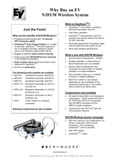


© Copyright 2026