1. society
2. crime
3. personal offense
4. assault

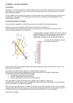
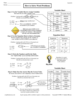
Appendix XIII. Sample Report
revised October 1, 2004
A sample lab report written by “Jane Doe” who had a lab partner
“John Jones” is on the following pages.
1
Appendix XIII: Sample Report
This page intentionally left without useful information
Appendix XIII: Sample Report
2
Free Fall Acceleration
Jane Doe
Department of Physics, Case Western Reserve University
Cleveland, OH 44016-7079
Abstract:
By using a brass object and commercially available tape timer, I have been able to measure
the magnitude of the acceleration due to gravity near the Earth’s surface. I have measured the
magnitude of the acceleration to be (9.54 ± 0.04) m/s2. The discrepancy between my results and
the accepted value of (9.81 ± 0.02) m/s2 is probably a result of the small amount of friction
between the paper tape and the tape timer. Our data also indicates that the acceleration was constant and that the equations of motion are valid for describing the position and velocity of the
brass weight as a function of time.
Introduction and Theory:
Newton’s law of gravitation allows one to calculate the gravitational force between two
massive bodies separated by a distance r. We can combine Newton’s law of gravitation with his
second law to determine that the magnitude of the acceleration g of a particle a distance re from
the Earth is
GM
g= 2e .
(1)
re
where G is the Universal Gravitational Constant and Me is the mass of the Earth. See References 1
and 2.
For objects moving near the Earth’s surface, we can make the approximation that the distance from the object to the center of the Earth is the radius of the Earth and remains constant, i.e.,
r ≈ re. With this approximation, the gravitational force on an object, and thus the acceleration,
remain constant.
If we take up as the positive y direction, the equations of motion reduce to a relatively
simple form. The expression for the position as a function of time is
y(t) =y0 + v0t -½gt2
(2)
and the expression for the velocity as a function of time is
v(t) = v0 - gt
(3)
where y0 and v0 are the position and velocity at time t = 0.
From Eq. 2, we can see that if we fit a quadratic equation to a plot of t vs. y, the secondorder slope will be -½g, or g will be negative twice the second-order slope. From Eq. 3, we can
see that if we fit a straight line to a plot of t vs. v, the slope of the line will be –g.
Jane Doe
1
Free Fall Acceleration
Experimental Procedure:
Tape timer
We used a 2-g binder clip to attach the
end of approximately 2 meters of paper tape to Ring stand
Paper tape
a brass object of mass 523 grams. We threaded
the other end of the paper tape through a Pasco
Scientific Tape Timer (model 9283). The timer
Brass object
was attached to a tall ring stand and was positioned above a catch bucket filled with sand.
See Figure 1.
To reduce the amount of friction between
Catch bucket
the paper tape and the tape timer, we held the
paper tape loosely above the timer and not
draped over the back or the front of the timer.
Prior to turning on the tape timer we allowed Figure 1: Apparatus used for experiment
any swinging motion of the object to dampen away. The timer was turned on so it was marking
the paper tape with small dots at a frequency of 40 Hz. The brass object was then released and the
force of gravity accelerated it downward into the catch bucket.
We then taped the paper tape to the table top (with care taken to ensure that the tape was
both straight and as stretched as it had been under the force of the brass object’s weight), and
measured and recorded the distance between the first dot and every subsequent dot with a twometer stick. These positions are listed in Table 1. We plotted the position and velocity of the brass
object as a function of time and compared the results to the theoretical values of position and
velocity.
Due to the size of the dots and parallax effects, I estimate that the uncertainty for the position measurements, δy, is ± 0.002 m. At the suggestion of my Teaching Assistant, Joe Smith, I
will adopt the manufacturer’s claimed accuracy in the time between successive dots of 0.001 s as
my uncertainty δ∆t. These are the values for the uncertainties I used for each data point in Table 1.
Results and Analysis:
The measurements of the position versus time are in Table 1. Also in Table 1 are the average velocities of the brass object as a function of time. These velocities were calculated by using
the relation
v = ∆y/∆t.
(4)
where ∆y is the distance between adjacent dots and ∆t is the time interval between dots, 25 ms,
which corresponds to 40 Hz.
Because the tape timer was turned on prior to releasing the brass object, I omitted the first
few points on the paper tape and did not include them in the tables or graphs. They were omitted
because they correspond either to dots printed prior to releasing the brass object or to those which
were printed during the initial release period where friction or forces due to the releasing mechanism (my fingers) may have affected the results. I also noted that the brass object hit the bucket
just before the tape came out of the tape timer. This circumstance is apparent in the data; the last
Jane Doe
2
Free Fall Acceleration
data point has a lower speed than the previous point. I therefore excluded the last data point from
our analysis.
Error Analysis:
As mentioned previously, my position measurements had an associated uncertainty of δy =
0.002 m. The velocity measurements can be determined by Eq. 4, where ∆y is the distance
between two adjacent points. Since each distance measurement, y, has its own uncertainty equal
to 0.002 m, I must calculate the uncertainty in ∆y, the difference between any two data points,
∆y = yi - yj
(5)
where yi and yj represent the positions of the two points i and j. The uncertainty of ∆y resulting
from the uncertainty in yi can be determined by the derivative method and is
δ∆y,i = δy,i .
(6)
Likewise, the uncertainty in ∆y as a result of the uncertainty in yj is
δ∆y,j = δy,j .
(7)
Adding these two uncertainties in quadrature gives the total uncertainty in ∆y,
((δ ) + (δ ) )
δ ∆y =
2
2
y ,i
y, j
(8)
Since this calculation only depends on the uncertainty of the measurement, δy, and not the measurement of y itself, we find that δ∆y is a constant for all points. Using the values of 0.002 m for
both δy,i and δ y,j, we find that δ∆y = 0.002828427 m ≈ 0.003 m.
I will now use the computational method to determine the uncertainty in the velocity measurement. I can calculate the average velocity of the brass object by applying Eq. 4. To determine
the uncertainty of that velocity, we calculated the uncertainty of the velocity resulting from the
uncertainty in the position and time measurements. The uncertainty of the velocity, δv,y due to the
uncertainty in the position is
δ v, y =
∆y + δ ∆y
∆t
−
∆y
.
∆t
(9)
Equation 9 reduces to
δ v, y =
δ ∆y
∆t
.
(10)
Here again I find that this quantity is a constant for all data points.
Jane Doe
3
Free Fall Acceleration
The uncertainty of the velocity measurement which results from the uncertainty in the time
measurement is
∆y
∆y
−
,
(11)
δ v ,t =
∆t ∆t + δ ∆t
which reduces to
∆y ⋅ δ ∆t
δ v ,t =
.
(12)
∆t (∆t + δ ∆t )
Adding Eqs. 10 and 12 in quadrature allows me to calculate the total uncertainty in the
velocity calculation:
δ ∆v =
((δ ) + (δ ) )
2
v, y
2
v ,t
(13)
Because of the ∆y dependence in Eq. 12, one would expect that the velocity calculation for
each point will have a different uncertainty associated with it.
I used the Origin software to calculate the uncertainty in the velocity and position of the
brass object in Table 1; they are also included in the position and velocity graphs, Figures 2 and 3.
Figures 2 and 3 are graphical representations of the measurements and calculations obtained
for this experiment. Figure 2 is a plot of the computed velocity versus time along with a linear fit
to the data. The linear fit corresponds to the equation of motion, Eq. 3, with a constant added to
compensate for any offset in the experimental data resulting from neglecting the first few data
points, as mentioned in the Procedure section. The slope of the linear fit is equal to the acceleration of the brass object and is a = (9.45 ± 0.07) m/s2.
Figure 3 shows the position as a function of time. Note that the error bars for the uncertainty
in the position are smaller than the data points. The solid curve is a polynomial fit to the experimental data. The polynomial fit used includes the zero-th and first order terms, A and B1*X, to
allow me to compensate for any offset in time and position resulting from neglecting the first few
data points as mentioned above. If we compare the equation of motion given in Eq. 2 to the polynomial fit of our data, we see that the coefficient B2 (4.77 ± 0.02) represents one-half of the
experimental acceleration. Using this value gives a magnitude of the acceleration due to gravity of
g = (9.54 ± 0.04) m/s2. The dashed curve in Figure 3 represents the theoretical position of the
brass object as a function of time using the accepted value of the magnitude of the acceleration,
g = (9.81 ± 0.02) m/s2. The theoretical curve has been shifted in time by 0.100 seconds to compensate for neglecting some initial data points.
Conclusions:
The data and linear fit in Figure 2 indicate that the magnitude of the acceleration of the brass
object was (9.45 ± 0.07) m/s2, which is 3.7% slower than the accepted value of (9.81 ± 0.02) m/s2.
This is a reasonable result because of the presence of a small amount of friction between the paper
tape and the tape timer, which would be a force opposing the direction of motion, thus decreasing
Jane Doe
4
Free Fall Acceleration
the acceleration. Another possible source of the discrepancy is air resistance, although the speeds
of the brass object are small enough so that this effect should be negligible. The linear fit to the
velocity versus time data is extremely good. This would imply that the equation of motion Eq. 3 is
sufficient in modeling the data we have obtained.
The polynomial fit of the data in Figure 3 gives a magnitude of the acceleration due to gravity of (9.54 ± 0.04) m/s2. This is a reasonable result, given the expected presence of friction as
described above. It is also agrees with the acceleration coefficient from the linear fit of the
velocity versus time data, Figure 2 (the results in Figs. 2 and 3 differ by only 0.09 ± 0.08 m/s2).
One can see that the polynomial fit used in Figure 3 is sufficiently good to support the claim that
the equation of motion, Eq. 2, is sufficient to describe the motion of the brass object for this
experiment. Because the polynomial fit takes into account that the object has a non-zero speed at
the first data point, I will adopt the value of g= (9.54 ± 0.04) m/s2 as my experimental value.
This experiment gave a magnitude of the gravitational acceleration near the surface of the
Earth to be g = (9.54 ± 0.04) m/s2. This value is significantly (7 standard deviations) smaller than
the accepted value of (9.81 ± 0.02) m/s2. The discrepancy between the experimental and accepted
values is probably due to the neglected friction between the paper tape and the tape timer. I have
also shown that the constant-acceleration kinematic equations of motion are valid for this
experiment.
Acknowledgements:
I would like to thank John Jones, CWRU Department of Physics, for his help in obtaining
the experimental data, preparing the figures, and checking my calculations. We also worked
together to develop Eqs. 5 through 13.
References:
1.
2.
Halliday, Resnick and Walker, Fundamentals of Physics, 6th edition, John Wiley and Sons,
Inc, 2001, pg. 295.
Schultz, D., General Physics I: Mechanics Lab Manual, CWRU Bookstore, Spring 2004.
Jane Doe
5
Free Fall Acceleration
Table 1: Experimental data
Time
(s)
t
Position
(m)
y
0.000
0.025
0.050
0.075
0.100
0.125
0.150
0.175
0.200
0.225
0.250
0.275
0.300
0.325
0.350
0.375
0.400
0.425
0.450
0.475
0.500
0.525
0.550
0
-0.0135
-0.033
-0.059
-0.091
-0.128
-0.172
-0.219
-0.273
-0.332
-0.397
-0.469
-0.546
-0.63
-0.721
-0.816
-0.918
-1.026
-1.142
-1.262
-1.389
-1.522
-1.654
Jane Doe
Uncertainty
in ∆y
(m)
δy
change in
position
(m)
∆y
δ∆y
velocity
(m/s)
v
0.002
0.002
0.002
0.002
0.002
0.002
0.002
0.002
0.002
0.002
0.002
0.002
0.002
0.002
0.002
0.002
0.002
0.002
0.002
0.002
0.002
0.002
0.002
-0.0135
-0.0195
-0.026
-0.032
-0.037
-0.044
-0.047
-0.054
-0.059
-0.065
-0.072
-0.077
-0.084
-0.091
-0.095
-0.102
-0.108
-0.116
-0.120
-0.127
-0.133
-0.132
0.003
0.003
0.003
0.003
0.003
0.003
0.003
0.003
0.003
0.003
0.003
0.003
0.003
0.003
0.003
0.003
0.003
0.003
0.003
0.003
0.003
0.003
-0.54
-0.78
-1.04
-1.28
-1.48
-1.76
-1.88
-2.16
-2.36
-2.60
-2.88
-3.08
-3.36
-3.64
-3.80
-4.08
-4.32
-4.64
-4.80
-5.08
-5.32
-5.28
Uncertainty
in y
(m)
6
Uncertainty
in velocity
(m/s)
δv
0.11
0.12
0.12
0.12
0.12
0.13
0.13
0.14
0.14
0.15
0.16
0.16
0.17
0.18
0.18
0.19
0.2
0.2
0.2
0.2
0.2
0.2
Free Fall Acceleration
Jane Doe
7
Free Fall Acceleration
Jane Doe
8
Free Fall Acceleration