1. No category

Chapter 10
Power and Sample size
Learning objectives
After completing this topic, you should be able to:
assess the power of a test or
determin the required sample size for a study.
Achieving these goals contributes to mastery in these course learning outcomes:
7. Distinguish between statistical significance and scientific relevance.
10. Identify and explain the statistical methods, assumptions, and limitations.
12. Make evidence-based decisions by constructing and deciding between
testable hypotheses using appropriate data and methods.
10.1
Power Analysis
The meaning of statistical power Power is the probability (1 − β)
of detecting an effect, given that the effect is really there. In other words,
it is the probability of correctly rejecting the null hypothesis when it is in fact
false. For example, let’s say that we have a simple study with drug A and a
placebo group, and that the drug truly is effective; the power is the probability
of finding a difference between the two groups. So, imagine that we had a power
of 1 − β = 0.8 and that this simple study was conducted many times. Having
power of 0.8 means that 80% of the time, we would get a statistically significant
difference between the drug A and placebo groups. This also means that 20%
10.1: Power Analysis
349
of the times that we run this experiment, we will not obtain a statistically
significant effect between the two groups, even though there really is an effect
in reality. That is, the probability of a Type-II error is β = 0.2.
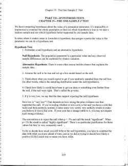
One-sample power figure Consider the plot below for a one-sample onetailed greater-than t-test. If the null hypothesis, H0 : µ = µ0, is true, then
the test statistic t is follows the null distribution indicated by the hashed area.
Under a specific alternative hypothesis, H1 : µ = µ1, the test statistic t follows
the distribution indicated by the solid area. If α is the probability of making
a Type-I error (rejecting H0 when it is true), then “crit. val.” indicates the
location of the tcrit value associated with H0 on the scale of the data. The
rejection region is the area under H0 that is at least as far as “crit. val.” is from
µ0. The power (1 − β) of the test is the green area, the area under H1 in the
rejection region. A Type-II error is made when H1 is true, but we fail to reject
H0 in the red region. (Note, for a two-tailed test the rejection region for both
tails under the H1 curve contribute to the power.)
#### One-sample power
# Power plot with two normal distributions
# http://stats.stackexchange.com/questions/14140/how-to-best-display-graphically-type-ii-bet
x <- seq(-4, 4, length=1000)
hx <- dnorm(x, mean=0, sd=1)
plot(x, hx, type="n", xlim=c(-4, 8), ylim=c(0, 0.5),
ylab = "",
xlab = "",
main= expression(paste("Type-II Error (", beta, ") and Power (", 1-beta, ")")), axes=FALSE)
#shift = qnorm(1-0.025, mean=0, sd=1)*1.7
shift = qnorm(1-0.05, mean=0, sd=1)*1.7 # one-tailed
xfit2 <- x + shift
yfit2 <- dnorm(xfit2, mean=shift, sd=1)
#axis(1, at = c(-qnorm(.025), 0, shift, -4),
#
labels = expression("p-value", 0, mu, -infinity ))
#axis(1, at = c(-qnorm(.025), 0, shift),
#
labels = expression((t[alpha/2]), mu[0], mu[1]))
axis(1, at = c(-qnorm(.05), 0, shift),
labels = expression("crit. val.", mu[0], mu[1]))
axis(1, at = c(-4, 4+shift),
labels = expression(-infinity, infinity ), lwd=1, lwd.tick=FALSE)
## Print null hypothesis area
350
Ch 10: Power and Sample size
#col_null = "#DDDDDD"
#polygon(c(min(x), x,max(x)), c(0,hx,0), col=col_null)
#lines(x, hx, lwd=2)
col_null = "#AAAAAA"
polygon(c(min(x), x,max(x)), c(0,hx,0), col=col_null, lwd=2, density=c(10, 40), angle=-45, bor
lines(x, hx, lwd=2, lty="dashed", col=col_null)
# The alternative hypothesis area
## The red - underpowered area
lb <- min(xfit2)
#ub <- round(qnorm(.975),2)
ub <- round(qnorm(.95),2)
col1 = "#CC2222"
i <- xfit2 >= lb & xfit2 <= ub
polygon(c(lb,xfit2[i],ub), c(0,yfit2[i],0), col=col1)
## The green area where the power is
col2 = "#22CC22"
i <- xfit2 >= ub
polygon(c(ub,xfit2[i],max(xfit2)), c(0,yfit2[i],0), col=col2)
# Outline the alternative hypothesis
lines(xfit2, yfit2, lwd=2)
axis(1, at = (c(ub, max(xfit2))), labels=c("", expression(infinity)),
col=col2, lwd=1, lwd.tick=FALSE)
#legend("topright", inset=.05, title="Color",
#
c("Null hypoteses","Type II error", "True"), fill=c(col_null, col1, col2), horiz=FALSE)
legend("topright", inset=.015, title="Color",
c("Null hypothesis","Type-II error", "Power"), fill=c(col_null, col1, col2),
angle=-45,
density=c(20, 1000, 1000), horiz=FALSE)
abline(v=ub, lwd=2, col="#000088", lty="dashed")
arrows(ub, 0.45, ub+1, 0.45, lwd=3, col="#008800")
arrows(ub, 0.45, ub-1, 0.45, lwd=3, col="#880000")
10.1: Power Analysis
351
Type−II Error (β) and Power (1 − β)
Color
Null hypothesis
Type−II error
Power
−∞
µ0
crit. val.
µ1
∞
Example: IQ drug Imagine that we are evaluating the effect of a putative memory enhancing drug. We have randomly sampled 25 people from a
population known to be normally distributed with a µ of 100 and a σ of 15.
We administer the drug, wait a reasonable time for it to take effect, and then
test our subjects’ IQ. Assume that we were so confident in our belief that the
drug would either increase IQ or have no effect that we entertained one-sided
(directional) hypotheses. Our null hypothesis is that after administering the
drug µ ≤ 100 and our alternative hypothesis is µ > 100.
These hypotheses must first be converted to exact hypotheses. Converting
the null is easy: it becomes µ = 100. The alternative is more troublesome.
If we knew that the effect of the drug was to increase IQ by 15 points, our
exact alternative hypothesis would be µ = 115, and we could compute power,
the probability of correctly rejecting the false null hypothesis given that µ is
really equal to 115 after drug treatment, not 100 (normal IQ). But if we already
352
Ch 10: Power and Sample size
knew how large the effect of the drug was, we would not need to do inferential
statistics. . .
One solution is to decide on a minimum nontrivial effect size. What
is the smallest effect that you would consider to be nontrivial? Suppose that
you decide that if the drug increases µIQ by 2 or more points, then that is a
nontrivial effect, but if the mean increase is less than 2 then the effect is trivial.
Now we can test the null of µ = 100 versus the alternative of µ = 102. Consider the previous plot. Let the left curve represent the distribution of sample
means if the null hypothesis were√true, µ = 100. This sampling distribution
has a µ = 100 and a σY¯ = 15/ 25 = 3. Let the right curve represent the
sampling distribution if the exact alternative hypothesis is true, µ = 102. Its
µ is 102 and, assuming the drug has no effect on the variance in IQ scores, also
has σY¯ = 3.
The green area in the upper tail of the null distribution (gray hatched curve)
is α. Assume we are using a one-tailed α of 0.05. How large would a sample
mean need be for us to reject the null? Since the upper 5% of a normal distribution extends from 1.645σ above the µ up to positive infinity, the sample mean
IQ would need be 100 + 1.645(3) = 104.935 or more to reject the null. What
are the chances of getting a sample mean of 104.935 or more if the alternative
hypothesis is correct, if the drug increases IQ by 2 points? The area under the
alternative curve from 104.935 up to positive infinity represents that probability, which is power. Assuming the alternative hypothesis is true, that µ = 102,
the probability of rejecting the null hypothesis is the probability of getting a
sample mean of 104.935 or more in a normal distribution with µ = 102, σ = 3.
Z = (104.935 − 102)/3 = 0.98, and P (Z > 0.98) = 0.1635. That is, power is
about 16%. If the drug really does increase IQ by an average of 2 points, we
have a 16% chance of rejecting the null. If its effect is even larger, we have a
greater than 16% chance.
Suppose we consider 5 (rather than 2) the minimum nontrivial effect size.
This will separate the null and alternative distributions more, decreasing their
overlap and increasing power. Now, Z = (104.935 − 105)/3 = −0.02, P (Z >
−0.02) = 0.5080 or about 51%. It is easier to detect large effects than
small effects.
10.1: Power Analysis
353
Suppose we conduct a 2-tailed test, since the drug could actually decrease
IQ; α is now split into both tails of the null distribution, 0.025 in each tail. We
shall reject the null if the sample mean is 1.96 or more standard errors away from
the µ of the null distribution. That is, if the mean is 100 + 1.96(3) = 105.88 or
more (or if it is 100−1.96(3) = 94.12 or less) we reject the null. The probability
of that happening if the alternative is correct (µ = 105) is: Z = (105.88 −
105)/3 = 0.29, P (Z > 0.29) = 0.3859, and P (Z < (94.12 − 105)/3) = P (Z <
−3.63) = 0.00014, for a total power = (1 − β) = 0.3859 + 0.00014, or about
39%. Note that our power is less than it was with a one-tailed test. If you
can correctly predict the direction of effect, a one-tailed test is
more powerful than a two-tailed test.
Consider what
√ would happen if you increased sample size to 100. Now
the σY¯ = 15/ 100 = 1.5. With the null and alternative distributions are
narrower, and should overlap less, increasing power. With σY¯ = 1.5 the sample
mean will need be 100 + (1.96)(1.5) = 102.94 (rather than 105.88 from before)
or more to reject the null. If the drug increases IQ by 5 points, power is:
Z = (102.94 − 105)/1.5 = −1.37, P (Z > −1.37) = 0.9147, or between 91 and
92%. Anything that decreases the standard error will increase
power. This may be achieved by increasing the sample size N or
by reducing the σ of the dependent variable. The σ of the dependent
variable may be reduced by reducing the influence of extraneous variables upon
the dependent variable (eliminating “noise” in the dependent variable makes it
easier to detect the signal).
Now consider what happens if you change the significance level, α. Let us
reduce α to 0.01. Now the sample mean must be 2.58 or more standard errors
from the null µ before we reject the null. That is, 100 + 2.58(1.5) = 103.87
(rather than 102.94 with α = 0.05). Under the alternative, Z = (103.87 −
105)/1.5 = −0.75, P (Z > −0.75) = 0.7734 or about 77%, less than it was
with α = 0.05. Reducing α reduces power.
Please note that all of the above analyses have assumed that we have used a
normally distributed test statistic, as Z = (Y¯ −µ0)/σY¯ will be if the dependent
variable is normally distributed in the population or if sample size is large
enough to invoke the central limit theorem (CLT). Remember that using Z
354
Ch 10: Power and Sample size
also requires that you know the population σ rather than estimating it from
the sample data. We more often estimate the population σ, using Student’s t
as the test statistic. If N is fairly large, Student’s t is nearly normal, so this is
no problem. For example, with a two-tailed α = 0.05 and N = 25, we went
out ±1.96 standard errors to mark off the rejection region. With Student’s
t on N − 1 = 24 df we should have gone out ±2.064 standard errors. But
1.96 versus 2.06 is a relatively trivial difference, so we should feel comfortable
with the normal approximation. If, however, we had N = 5, df = 4, critical
t = ±2.776, then the normal approximation would not do. A more complex
analysis would be needed.
10.2
Effect size
For the one-sample test, the effect size in σ units is d = (µ1 − µ0)/σ. For our
IQ problem with minimum nontrivial effect size at 5 IQ points, d = (105 −
100)/15 = 1/3. Cohen’s1 conventions for small, medium, and large effects for
a two-sample difference test between two means is in the table below.
One- or two-sample difference of means
Size of effect d
% variance
small
0.2
1
medium
0.5
6
large
0.8
16
Cohen has conventions for other tests (correlation, contingency tables, etc.),
but they should be used with caution.
What is a small or even trivial effect in one context may be a large effect
in another context. For example, Rosnow and Rosenthal (1989) discussed a
1988 biomedical research study on the effects of taking a small, daily dose of
aspirin. Each participant was instructed to take one pill a day. For about
half of the participants the pill was aspirin, for the others it was a placebo.
The dependent variable was whether or not the participant had a heart attack
during the study. In terms of a correlation coefficient, the size of the observed
1
Cohen, J. (1988). Statistical power analysis for the behavior sciences. (2nd ed.). Hillsdale, NJ:
Erlbaum.
10.3: Sample size
355
effect was r = 0.034. In terms of percentage of variance explained, that is
0.12%. In other contexts this might be considered a trivial effect, but it this
context it was so large an effect that the researchers decided it was unethical
to continue the study and the contacted all of the participants who were taking
the placebo and told them to start taking aspirin every day.
10.3
Sample size
Before you can answer the question ”how many subjects do I need,” you will
have to answer several other questions, such as:
ˆ How much power do I want?
ˆ What is the likely size (in the population) of the effect I am trying to
detect, or, what is smallest effect size that I would consider of importance?
ˆ What criterion of statistical significance will I employ?
ˆ What test statistic will I employ?
ˆ What is the standard deviation (in the population) of the criterion variable?
ˆ For correlated samples designs, what is the correlation (in the population)
between groups?
If one considers Type I and Type II errors equally serious, then one should have
enough power to make α = β. If employing the traditional 0.05 criterion of
statistical significance, that would mean you should have 95% power. However,
getting 95% power usually involves expenses too great – that is, too many
samples.
A common convention is to try to get at least enough data to have 80%
power. So, how do you figure out how many subjects you need to have the
desired amount of power. There are several methods, including:
ˆ You could buy an expensive, professional-quality software package to do
the power analysis.
ˆ You could buy an expensive, professional-quality book on power analysis
and learn to do the calculations yourself and/or to use power tables and
figures to estimate power.
ˆ You could try to find an interactive web page on the Internet that will do
356
Ch 10: Power and Sample size
the power analysis for you. This is probably fine, but be cautious.
ˆ You could download and use the G Power program, which is free, not too
difficult to use, and generally reliable (this is not to say that it is error
free).
ˆ You could use the simple guidelines provided in Jacob Cohen’s “A Power
Primer” (Psychological Bulletin, 1992, 112, 155-159).
The plots below indicate the amount of power for a given effect size and
sample size for a one-sample t-test and ANOVA test. This graph makes clear
the diminishing returns you get for adding more and more subjects if you already
have moderate to high power. For example, let’s say we’re doing a one-sample
test and we an effect size of 0.2 and have only 10 subjects. We can see that we
have a power of about 0.15, which is really, really low. Going to 25 subjects
increases our power to about 0.25, and to 100 subjects increases our power to
about 0.6. But if we had a large effect size of 0.8, 10 subjects would already
give us a power of about 0.8, and using 25 or 100 subjects would both give a
power at least 0.98. So each additional subject gives you less additional power.
This curve also illustrates the “cost” of increasing your desired power from 0.8
to 0.98.
# Power curve plot for one-sample t-test with range of sample sizes
# http://stackoverflow.com/questions/4680163/power-vs-effect-size-plot/4680786#4680786
P
fVals
dVals
#nn
nn
alpha
<- 3
<- seq(0, 1.2, length.out=100)
<- seq(0, 3, length.out=100)
<- seq(10, 25, by=5)
<- c(5,10,25,100)
<- 0.05
# number of groups for ANOVA
# effect sizes f for ANOVA
# effect sizes d for t-Test
# group sizes
# group sizes
# test for level alpha
# function to calculate one-way ANOVA power for given group size
getFPow <- function(n) {
critF <- qf(1-alpha, P-1, P*n - P) # critical F-value
# probabilities of exceeding this F-value given the effect sizes f
# P*n*fVals^2 is the non-centrality parameter
1-pf(critF, P-1, P*n - P, P*n * fVals^2)
}
# function to calculate one-sample t-Test power for given group size
getTPow <- function(n) {
critT <- qt(1-alpha, n-1)
# critical t-value
# probabilities of exceeding this t-value given the effect sizes d
10.3: Sample size
357
# sqrt(n)*d is the non-centrality parameter
1-pt(critT, n-1, sqrt(n)*dVals)
}
powsF <- sapply(nn, getFPow)
powsT <- sapply(nn, getTPow)
# ANOVA power for for all group sizes
# t-Test power for for all group sizes
#dev.new(width=10, fig.height=5)
par(mfrow=c(1, 2))
matplot(dVals, powsT, type="l", lty=1, lwd=2, xlab="effect size d",
ylab="Power", main="Power one-sample t-test", xaxs="i",
xlim=c(-0.05, 1.1), col=c("blue", "red", "darkgreen", "green"))
#legend(x="bottomright", legend=paste("N =", c(5,10,25,100)), lwd=2,
#
col=c("blue", "red", "darkgreen", "green"))
legend(x="bottomright", legend=paste("N =", nn), lwd=2,
col=c("blue", "red", "darkgreen", "green"))
#matplot(fVals, powsF, type="l", lty=1, lwd=2, xlab="effect size f",
#
ylab="Power", main=paste("Power one-way ANOVA, ", P, " groups", sep=""), xaxs="i",
#
xlim=c(-0.05, 1.1), col=c("blue", "red", "darkgreen", "green"))
##legend(x="bottomright", legend=paste("Nj =", c(10, 15, 20, 25)), lwd=2,
##
col=c("blue", "red", "darkgreen", "green"))
#legend(x="bottomright", legend=paste("Nj =", nn), lwd=2,
#
col=c("blue", "red", "darkgreen", "green"))
library(pwr)
pwrt2 <- pwr.t.test(d=.2,n=seq(2,100,1),
sig.level=.05,type="one.sample", alternative="two.sided")
pwrt3 <- pwr.t.test(d=.3,n=seq(2,100,1),
sig.level=.05,type="one.sample", alternative="two.sided")
pwrt5 <- pwr.t.test(d=.5,n=seq(2,100,1),
sig.level=.05,type="one.sample", alternative="two.sided")
pwrt8 <- pwr.t.test(d=.8,n=seq(2,100,1),
sig.level=.05,type="one.sample", alternative="two.sided")
#plot(pwrt£n, pwrt£power, type="b", xlab="sample size", ylab="power")
matplot(matrix(c(pwrt2$n,pwrt3$n,pwrt5$n,pwrt8$n),ncol=4),
matrix(c(pwrt2$power,pwrt3$power,pwrt5$power,pwrt8$power),ncol=4),
type="l", lty=1, lwd=2, xlab="sample size",
ylab="Power", main="Power one-sample t-test", xaxs="i",
xlim=c(0, 100), ylim=c(0,1), col=c("blue", "red", "darkgreen", "green"))
legend(x="bottomright", legend=paste("d =", c(0.2, 0.3, 0.5, 0.8)), lwd=2,
col=c("blue", "red", "darkgreen", "green"))
358
Ch 10: Power and Sample size
0.6
0.0
0.2
0.4
0.6
effect size d
0.8
1.0
d = 0.2
d = 0.3
d = 0.5
d = 0.8
0.0
N=5
N = 10
N = 25
N = 100
0.2
0.4
Power
0.6
0.2
0.4
Power
0.8
0.8
1.0
Power one−sample t−test
1.0
Power one−sample t−test
0
20
40
60
80
100
sample size
Reasons to do a power analysis There are several of reasons why one
might do a power analysis. (1) Perhaps the most common use is to determine
the necessary number of subjects needed to detect an effect of a given size. Note
that trying to find the absolute, bare minimum number of subjects needed in the
study is often not a good idea. (2) Additionally, power analysis can be used to
determine power, given an effect size and the number of subjects available. You
might do this when you know, for example, that only 75 subjects are available
(or that you only have the budget for 75 subjects), and you want to know if you
will have enough power to justify actually doing the study. In most cases, there
is really no point to conducting a study that is seriously underpowered. Besides
the issue of the number of necessary subjects, there are other good reasons for
doing a power analysis. (3) For example, a power analysis is often required as
part of a grant proposal. (4) And finally, doing a power analysis is often just
part of doing good research. A power analysis is a good way of making sure
that you have thought through every aspect of the study and the statistical
analysis before you start collecting data.
10.3: Sample size
359
Limitations Despite these advantages of power analyses, there are some
limitations. (1) One limitation is that power analyses do not typically generalize
very well. If you change the methodology used to collect the data or change
the statistical procedure used to analyze the data, you will most likely have to
redo the power analysis. (2) In some cases, a power analysis might suggest a
number of subjects that is inadequate for the statistical procedure. For example
(beyond the scope of this class), a power analysis might suggest that you need
30 subjects for your logistic regression, but logistic regression, like all maximum
likelihood procedures, require much larger sample sizes. (3) Perhaps the most
important limitation is that a standard power analysis gives you a “best case
scenario” estimate of the necessary number of subjects needed to detect the
effect. In most cases, this “best case scenario” is based on assumptions and
educated guesses. If any of these assumptions or guesses are incorrect, you may
have less power than you need to detect the effect. (4) Finally, because power
analyses are based on assumptions and educated guesses, you often get a range
of the number of subjects needed, not a precise number. For example, if you do
not know what the standard deviation of your outcome measure will be, you
guess at this value, run the power analysis and get X number of subjects. Then
you guess a slightly larger value, rerun the power analysis and get a slightly
larger number of necessary subjects. You repeat this process over the plausible
range of values of the standard deviation, which gives you a range of the number
of subjects that you will need.
Other considerations After all of this discussion of power analyses and
the necessary number of subjects, we need to stress that power is not the only
consideration when determining the necessary sample size. For example, different researchers might have different reasons for conducting a regression analysis.
(1) One might want to see if the regression coefficient is different from zero, (2)
while the other wants to get a very precise estimate of the regression coefficient
with a very small confidence interval around it. This second purpose requires a
larger sample size than does merely seeing if the regression coefficient is different
from zero. (3) Another consideration when determining the necessary sample
size is the assumptions of the statistical procedure that is going to be used (e.g.,
360
Ch 10: Power and Sample size
parametric vs nonparametric procedure). (4) The number of statistical tests
that you intend to conduct will also influence your necessary sample size: the
more tests that you want to run, the more subjects that you will need (multiple comparisons). (5) You will also want to consider the representativeness
of the sample, which, of course, influences the generalizability of the results.
Unless you have a really sophisticated sampling plan, the greater the desired
generalizability, the larger the necessary sample size.
10.4
Power calculation via simulation
Using the principles of the bootstrap (to be covered later) we can estimate
statistical power through simulation.
Example: IQ drug, revisited Recall that we sample N = 25 people
from a population known to be normally distributed with a µ of 100 and a σ
of 15. Consider the first one-sided alternative H0 : µ = 100 and H1 : µ > 100.
Assume the minimum nontrivial effect size was that the drug increases µIQ
by 2 or more points, so that the specific alternative to consider is H1 : µ = 102.
What is the power of this test?
We already saw how to calculate this analytically. To solve this computationally, we need to simulate samples of N = 25 from the alternative distribution (µ = 102 and σ = 15) and see what proportion of the time we correctly
reject H0.
#### Example: IQ drug, revisited
# R code to simulate one-sample one-sided power
# Strategy:
# Do this R times:
#
draw a sample of size N from the distribution specified by the alternative hypothesis
#
That is, 25 subjects from a normal distribution with mean 102 and sigma 15
#
Calculate the mean of our sample
#
Calculate the associated z-statistic
#
See whether that z-statistic has a p-value < 0.05 under H0: mu=100
#
If we reject H0, then set reject = 1, else reject = 0.
# Finally, the proportion of rejects we observe is the approximate power
n
mu0
<- 25;
<- 100;
# sample size of 25
# null hypothesis mean of 100
10.4: Power calculation via simulation
361
mu1
<- 102;
#mu1
<- 105;
sigma <- 15;
# alternative mean of 102
# alternative mean of 105
# standard deviation of normal population
alpha <- 0.05;
# significance level
R
<- 10000;
# Repetitions to draw sample and see whether we reject H0
#
The proportion of these that reject H0 is the power
reject <- rep(NA, R);
# allocate a vector of length R with missing values (NA)
#
to fill with 0 (fail to reject H0) or 1 (reject H0)
for (i in 1:R) {
sam <- rnorm(n, mean=mu1, sd=sigma);
ybar <- mean(sam);
# sam is a vector with 25 values
# Calculate the mean of our sample sam
z <- (ybar - mu0) / (sigma / sqrt(n)); # z-statistic (assumes we know sigma)
# we could also have calculated the t-statistic, here
pval <- 1-pnorm(z);
# one-sided right-tail p-value
#
pnorm gives the area to the left of z
#
therefore, the right-tail area is 1-pnorm(z)
if (pval < 0.05) {
reject[i] <- 1; # 1 for correctly rejecting H0
} else {
reject[i] <- 0; # 0 for incorrectly fail to reject H0
}
}
power <- mean(reject);
power
# the average reject (proportion of rejects) is the power
## [1] 0.166
# 0.1655
# 0.5082
for mu1=102
for mu1=105
Our simulation (this time) with µ1 = 102 gave a power of 0.166 (exact
answer is P (Z > 0.98) = 0.1635). Rerunning with µ1 = 105 gave a power
of 0.5082 (exact answer is P (Z > −0.02) = 0.5080). Our simulation wellapproximates the true value, and the power can be made more precise by increasing the number of repetitions calculated. However, two to three decimal
precision is quite sufficient.
Example: Head breadth Recall the head breadth example in Chapter 3
comparing maximum head breadths (in millimeters) of modern day Englishmen
with ancient Celts. The data are summarized below.
362
Ch 10: Power and Sample size
Descriptive Statistics: ENGLISH, CELTS
Variable
N
Mean SE Mean StDev Minimum
ENGLISH
18 146.50
1.50
6.38
132.00
CELTS
16 130.75
1.36
5.43
120.00
Q1
141.75
126.25
Median
147.50
131.50
Q3
150.00
135.50
Maximum
158.00
138.00
Imagine that we don’t have the information above. Imagine we have been
invited to a UK university to take skull measurements for 18 modern day Englishmen, and 16 ancient Celts. We have some information about modern day
skulls to use as prior information for measurement mean and standard deviation. What is the power to observe a difference between the populations? Let’s
make some reasonable assumptions that allows us to be a bit conservative. Let’s
assume the sampled skulls from each of our populations is a random sample
with common standard deviation 7mm, and let’s assume we can’t get the full
sample but can only measure 15 skulls from each population. At a significance
level of α = 0.05, what is the power for detecting a difference of 5, 10, 15, 20,
or 25 mm?
The theoretical two-sample power result is not too hard to derive (and is
available in text books), but let’s simply compare the power calculated exactly
and by simulation.
For the exact result we use R library pwr. Below is the function call as well
as the result. Note that we specified multiple effect sizes (diff/SD) in one call
of the function.
# R code to compute exact two-sample two-sided power
library(pwr) # load the power calculation library
pwr.t.test(n = 15,
d = c(5,10,15,20,25)/7,
sig.level = 0.05,
power = NULL,
type = "two.sample",
alternative = "two.sided")
##
##
Two-sample t
##
##
n =
##
d =
##
sig.level =
##
power =
##
alternative =
##
## NOTE: n is number
test power calculation
15
0.7143, 1.4286, 2.1429, 2.8571, 3.5714
0.05
0.4717, 0.9652, 0.9999, 1.0000, 1.0000
two.sided
in *each* group
10.4: Power calculation via simulation
363
To simulate the power under the same circumstances, we follow a similar
strategy as in the one-sample example.
# R code to simulate two-sample two-sided power
# Strategy:
# Do this R times:
#
draw a sample of size N from the two hypothesized distributions
#
That is, 15 subjects from a normal distribution with specified means and sigma=7
#
Calculate the mean of the two samples
#
Calculate the associated z-statistic
#
See whether that z-statistic has a p-value < 0.05 under H0: mu_diff=0
#
If we reject H0, then set reject = 1, else reject = 0.
# Finally, the proportion of rejects we observe is the approximate power
n
mu1
mu2
sigma
<- 15;
# sample size of 25
<- 147;
# null hypothesis English mean
<- c(142, 137, 132, 127, 122); # Celt means
<7;
# standard deviation of normal population
alpha <- 0.05;
# significance level
R
# Repetitions to draw sample and see whether we reject H0
#
The proportion of these that reject H0 is the power
<- 2e4;
power <- rep(NA,length(mu2));
for (j in 1:length(mu2)) {
reject <- rep(NA, R);
# allocate a vector to store the calculated power in
# do for each value of mu2
# allocate a vector of length R with missing values (NA)
#
to fill with 0 (fail to reject H0) or 1 (reject H0)
for (i in 1:R) {
sam1 <- rnorm(n, mean=mu1
, sd=sigma);
sam2 <- rnorm(n, mean=mu2[j], sd=sigma);
ybar1 <- mean(sam1);
ybar2 <- mean(sam2);
# English sample
# Celt sample
# Calculate the mean of our sample sam
# Calculate the mean of our sample sam
# z-statistic (assumes we know sigma)
# we could also have calculated the t-statistic, here
z <- (ybar2 - ybar1) / (sigma * sqrt(1/n+1/n));
pval.Left <- pnorm(z);
# area under left tail
pval.Right <- 1-pnorm(z); # area under right tail
# p-value is twice the smaller tail area
pval <- 2 * min(pval.Left, pval.Right);
if (pval < 0.05) {
reject[i] <- 1; # 1 for correctly rejecting H0
} else {
reject[i] <- 0; # 0 for incorrectly fail to reject H0
364
Ch 10: Power and Sample size
}
}
# the average reject (proportion of rejects) is the power
power[j] <- mean(reject);
}
power
## [1] 0.4928 0.9765 1.0000 1.0000 1.0000
Note the similarity between power calculated using both the exact and simulation methods. If there is a power calculator for your specific problem, it is
best to use that because it is faster and there is no programming. However,
using the simulation method is better if we wanted to entertain different sample sizes with different standard deviations, etc. There may not be a standard
calculator for our specific problem, so knowing how to simulate the power can
be valuable.
Mean
Sample size
Power
µE µC diff SD nE
nC exact simulated
147 142
5 7 15
15 0.4717
0.4928
147 137 10 7 15
15 0.9652
0.9765
147 132 15 7 15
15 0.9999
1
147 127 20 7 15
15 1.0000
1
147 122 25 7 15
15 1.0000
1