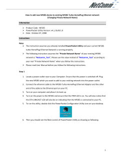
Conjoint Analysis
This module covers how to interpret the results of a
conjoint study, including the topics of attribute importance,
willingness-to-pay, statistical validity, customer feature
trade-offs, and market share prediction.
Author: Ronald T. Wilcox
Marketing Metrics Reference: Chapter 4
© 2010-14 Ronald T. Wilcox and Management by the Numbers, Inc.
Consumers have complex preferences!
We want to be able to understand the
preferences of our customers and potential
customers for the products and services we are
offering or may consider offering.
MEASURING CONSUMER PREFERENCES
Measuring Consumer Preference
We can examine the choices people make to
uncover how they value the different features of
a product or service.
MBTN | Management by the Numbers
2
We seek to determine how consumers value the different features that
make up a product and the tradeoffs they are willing to make among the
different features when they make product choices. Sometimes these
hidden drivers of choice are not apparent to the consumers themselves.
Definition
CONJOINT ANALYSIS - DEFINITION
Conjoint Analysis - Definition
Conjoint analysis is a statistical technique used in marketing research to
measure how people value the different features or attributes that
comprise a multi-attribute product or service.
MBTN | Management by the Numbers
3
Conjoint Analysis can help when:
1. The product or service being examined is comprised of multiple
attributes or potential attributes.
•
Example: When deciding on a new car a consumer may consider
price, fuel economy, size of the engine, etc.
2. The various values or levels an attribute are well understood by
consumers and can be described in unambiguous terms.
•
WHEN CONJOINT ANALYSIS CAN HELP
When Conjoint Analysis Can Help
Example: “24 Miles per Gallon” is unambiguous, “Great New
Styling” is ambiguous.
3. It is reasonable to believe that consumers strongly
consider these attributes when making product choices.
MBTN | Management by the Numbers
4
Show consumers a series of hypothetical products defined by their
attributes.
• Ask the respondent to pick the product they like the best.
• Some types of conjoint analysis ask consumers to rank
products according to their preferences rather than choosing a
single most-preferred product.
HOW CONJOINT ANALYSIS WORKS
How Conjoint Analysis Works
Gather multiple observations per person and include many people in
the study.
• Use responses to estimate the preferences for various features.
• Marketing researchers generally used specialized software to
come up with these estimates.
MBTN | Management by the Numbers
5
Conjoint analysis begins with an experimental design. This design
includes all attributes, and the values of the attributes, that will be
tested. Conjoint analysis distinguishes between attributes and what
are generally called “levels.”
An attribute is pretty self-explanatory. It could be something like price,
color, horsepower, material used for the upholstery, or presence of
sunroof.
EXPERIMENTAL DESIGN
The Experimental Design
A “level” is the specific value or realization of the attribute. For
example, the attribute “color” may have the levels “red,” “blue,” and
“yellow” while the attribute “presence of a sunroof” will have levels
“yes” and “no.”
Before a researcher begins to collect data it is important to write down
all of the levels of each attribute to be tested. Commercially available
software packages will require that the user provide these as input.
MBTN | Management by the Numbers
6
Staying with our car example, an experimental design might look
like the following:
Attribute:
Levels:
Price
Brand
Horsepower
Upholstery
Sunroof
$23,000
Toyota
220 HP
Cloth
Yes
$25,000
$27,000
Volkswagen
Saturn
250 HP
280 HP
Leather
No
$29,000
Kia
EXPERIMENTAL DESIGN
The Experimental Design
It is important to note that any level of an attribute might be
combined with any other level of another attribute during the
experiment. For example, the consumer might be presented a
hypothetical product that a Volkswagen, priced at $29,000, has
220 horsepower, a leather interior and a sunroof.
This is a very simple design that contains a total of 15 attribute
levels. Real world designs often contain more attributes and
levels than are presented here.
MBTN | Management by the Numbers
7
The basic results of a conjoint analysis are the estimated attribute
level utilities or part-worths. These correspond to the average
consumer preference for the level of any given attribute.
Attribute
Price
Brand
Horsepower
Upholstery
Sunroof
Level
$23,000
$25,000
$27,000
$29,000
Toyota
Volkswagen
Saturn
Kia
220 HP
250 HP
280 HP
Cloth
Leather
Yes
No
Utility (Part-worth)
2.10
1.15
-1.56
-1.69
0.75
0.65
-0.13
-1.27
-2.24
1.06
1.18
-1.60
1.60
0.68
-0.68
t-value
14.00
7.67
10.40
11.27
5.00
4.33
0.87
8.47
14.93
7.07
7.87
10.67
10.67
4.53
4.53
MBTN | Management by the Numbers
BASIC CONJOINT ANALYSIS OUTPUT
Basic Conjoint Analysis Output
8
Note: Within a given attribute, the estimated utilities are generally scaled
in such a way that they add up to zero. So, a negative number does not
mean that the given level has “negative utility,” It just means that this level
is on average less preferred than a level with an estimated utility that is
positive.
Attribute
Price
Brand
Horsepower
Upholstery
Sunroof
Level
$23,000
$25,000
$27,000
$29,000
Toyota
Volkswagen
Saturn
Kia
220 HP
250 HP
280 HP
Cloth
Leather
Yes
No
Utility (Part-worth)
2.10
1.15
-1.56
-1.69
0.75
0.65
-0.13
-1.27
-2.24
1.06
1.18
-1.60
1.60
0.68
-0.68
t-value
14.00
7.67
10.40
11.27
5.00
4.33
0.87
8.47
14.93
7.07
7.87
10.67
10.67
4.53
4.53
MBTN | Management by the Numbers
BASIC CONJOINT ANALYSIS OUTPUT
Basic Conjoint Analysis Output
9
Conjoint analysis output is also often accompanied by t-values, a
standard metric for evaluating statistical significance. Because of the
way conjoint utilities are scaled, the standard interpretation of t-values
can yield misleading results.
For example, the level “Saturn” of the attribute “Brand” has a t-value
of 0.87. In general, a t-value of this magnitude would fail a test of
statistical significance. However, this t-value is generated because
within the attribute “Brand” the level “Saturn” has neither a very high
nor very low relative preference. It is basically in the middle in terms of
overall preference.
Attribute
Brand
Level
Toyota
Volkswagen
Saturn
Kia
Utility (Part-worth)
0.75
0.65
-0.13
-1.27
BASIC CONJOINT ANALYSIS OUTPUT
Basic Conjoint Analysis Output
t-value
5.00
4.33
0.87
8.47
MBTN | Management by the Numbers
10
Because of the scaling, levels that have more moderate levels of
preference within a given attribute are likely to have estimated utilities close
to zero which will tend to produce very low t-values (recall that the t-test is
measuring the probability that the true value of a parameter is not different
from zero).
Attribute
Price
Brand
Horsepower
Upholstery
Sunroof
Level
$23,000
$25,000
$27,000
$29,000
Toyota
Volkswagen
Saturn
Kia
220 HP
250 HP
280 HP
Cloth
Leather
Yes
No
Utility (Part-worth)
2.10
1.15
-1.56
-1.69
0.75
0.65
-0.13
-1.27
-2.24
1.06
1.18
-1.60
1.60
0.68
-0.68
t-value
14.00
7.67
10.40
11.27
5.00
4.33
0.87
8.47
14.93
7.07
7.87
10.67
10.67
4.53
4.53
MBTN | Management by the Numbers
BASIC CONJOINT ANALYSIS OUTPUT
Basic Conjoint Analysis Output
11
The utility of any product we might be considering is simply the sum of
the utilities of its attribute levels. For example, a Toyota with 280
horsepower, leather interior, no sunroof and a price of $23,000 has a
utility of 0.75 + 1.18 + 1.60 - 0.68 + 2.10 = 4.95
BASIC INTERPRETATION
Basic Interpretation
As a natural consequence of this additive property, relatively large
positive numbers can be interpreted as adding a lot to overall product
utility. Negative utilities indicate less desired levels of attributes with the
most negative being the least desired.
Utility estimates are directly comparable across attributes. For
example, having a leather rather than cloth interior (1.60 versus -1.60)
adds more to overall product utility than having a sunroof (0.68 versus 0.68).
MBTN | Management by the Numbers
12
Intuitively, the difference in the utilities between the most preferred and
least preferred level within an attribute tells you something about how
important this attribute is in the consumer choice process.
In order to calculate the importance of any given attribute, you just take
the difference between the highest and lowest utility level of that
attribute and divide this by the sum of the differences between the
highest and lowest utility level for all attributes (including the one in
question). The resulting number will always lie between zero and one
and is generally interpreted as the percent decision weight of an
attribute in the overall choice process.
MBTN | Management by the Numbers
INTERPRETATION: ATTRIBUTE IMPORTANCE
Interpretation: Attribute Importance
13
Consider the attribute “horsepower.” What is its overall importance in
the choice process?
I Horsepower =
1.18 + 2.24
=.25
((2.10 + 1.69) + (0.75 + 1.27) + (1.18 + 2.24) + (1.60 + 1.60) + (0.68 + 0.68))
Insight:
INTERPRETATION: ATTRIBUTE IMPORTANCE
Interpretation: Attribute Importance
This means that 25% of the overall decision weight of consumers is on
horsepower. The greater this percentage, the greater the decision weight.
An analogous calculation for “Price” is about 27%, “Brand” about 15%,
“Sunroof” about 10%, and “Upholstery” about 23%. These numbers
provide a very intuitive metric for thinking about the importance of each
attribute in the decision process.
For practice, you might want to calculate these other important values.
MBTN | Management by the Numbers
14
Question 1: Consider a Toyota at a price of $23,000 with 280
horsepower, leather interior and no sunroof. How much would the
average consumer be willing-to-pay if a sunroof were added?
The car without the sunroof has a utility of 0.75 + 1.18 + 1.60 - 0.68 +
2.10 = 4.95. If we add the sunroof this increases the overall utility to
0.75 + 1.18 + 1.60 + 0.68 + 2.10 = 6.31 for a difference of 6.31 – 4.95
= 1.36.
This implies that we can reduce the utility of price by 1.36 and the
average consumer would be just as happy as before the sunroof was
installed. By carefully examining the estimated utilities for the different
levels of price we can solve for this new price!
MBTN | Management by the Numbers
INTERPRETATION: WILLINGNESS-TO-PAY
Interpretation: Willingness-to-pay
15
Answer: To find out how much the price can be raised we must convert
the change in utility to a change in price. We do this by first noting how
much the original car costs $23,000 and the utility associate with that figure,
2.10. We know that we can reduce the price utility by 1.36. This is equivalent
to saying that we can reduce the price utility to 2.10 – 1.36 = 0.74. By
referring to the utility estimates we can immediately see that this implies a
price between $25,000 and $27,000 because -1.56 < 0.74 < 1.15. In fact, if
we assume a linear relationship between price and utility in the range
between $25,000 and $27,000 we can solve for the exact price by
performing a linear interpolation within this range.
$25,000 +
WILLINGNESS-TO-PAY (CONTINUED)
Willingness-to-pay (continued)
1.15 − 0.74
* $2,000 = $25,302.58
1.15 − (−1.56)
Utility spread between
the two tested price
points ($25K and $27K).
Utility spread
between $25K and
the target utility.
MBTN | Management by the Numbers
16
$25,000 +
1.15 − 0.74
* $2,000 = $25,302.58
1.15 − (−1.56)
Utility spread between
the two tested price
points ($25K and $27K).
Utility spread
between $25K and
the target utility.
WILLINGNESS-TO-PAY (CONTINUED)
Willingness-to-pay (continued)
This implies that if the sunroof is added and the price of the vehicle is
raised from $23,000 to about $25,300 the average consumer would be
indifferent between the two vehicles. Managerially, it provides the
maximum amount the price can be raised if the new feature is included
without compromising market share. In this case the maximum is $2,300
($25,300 - $23,000).
MBTN | Management by the Numbers
17
Calculating willingness-to-pay for a feature upgrade is an example of
one particular type of trade-off analysis. A consumer is trading off
money (price) for something better on another dimension of the
product.
Insight:
More generally, we can use conjoint analysis any trade-off a consumer
would be willing to make among the attributes that are tested in the
experiment. These estimated trade-offs become important determinants
of design when a company is developing new products or services.
MBTN | Management by the Numbers
INTERPRETATION: TRADE-OFF ANALYSIS
Interpretation: Trade-off analysis
18
Question 2: Suppose Volkswagen is currently selling a car for
$25,000 that comes standard with a 250 HP engine, cloth interior and
no sunroof. If Volkswagen upgrades this vehicle to have a leather
interior, how much power (horsepower) would the average consumer
be willing to give up to get this upgrade?
This analysis proceeds much like the willingness-to-pay analysis. First,
we must determine how much additional utility the average consumer
gets from the upgrade to a leather interior.
MBTN | Management by the Numbers
INTERPRETATION: TRADE-OFF ANALYSIS
Interpretation: Trade-off analysis
19
Answer:
The additional utility for the leather interior is the difference between the
utility for the leather and cloth interior, 1.6 + 1.6 = 3.2. Converting this to
horsepower, exactly as we did in the willingness-to-pay problem, yields:
250 HP −
1.6 − (−1.6)
* (250 − 220) HP = 221HP
1.06 − (−2.24)
Utility spread between
the two relevant levels
(250HP and 220HP).
INTERPRETATION: TRADE-OFF ANALYSIS
Interpretation: Trade-off analysis
Utility spread between
leather and cloth
interiors.
The average consumer would be willing to reduce overall horsepower
from 250HP to 221HP, a reduction of 29HP, to get a leather interior.
MBTN | Management by the Numbers
20
Another common application is forecasting market share. In order to
use conjoint analysis output for this kind of prediction two conditions
must be satisfied.
1. The company must know the other products, besides their own
offering, that a consumer is likely to consider when making a
selection in the relevant category.
2. Each of these competitive products’ important features must be
included in the experimental design. In other words, you must be
able to calculate the utility of not only your own product offering
but that of the competitive products as well.
MBTN | Management by the Numbers
INTERPRETATION: MARKET SHARE FORECASTING
Interpretation: Market Share Forecasting
21
Market share prediction relies on the use of a multinomial logit model.
The basic form of the logit model is:
Sharei =
eU i
∑ j =1 e
n
U
j
where
• Ui is the estimated utility of product i (sum of attribute utilities)
• Uj is the estimated utility of product j
• n is the total number of products in the competitive
set, including product i.
INTERPRETATION: MARKET SHARE FORECASTING
Interpretation: Market Share Forecasting
Yes, that e you see really is the one you sort of remember from high
school, the base of the natural logarithm (approximately 2.718).
MBTN | Management by the Numbers
22
Question 3: Suppose we are considering marketing a car with the
following profile: Saturn; $23,000; 220 HP; Cloth interior; No sunroof.
We believe that when consumers consider our car they will also
consider purchasing cars that are currently on the market with the
following profiles:
•
•
•
$27,000; Toyota; 250 HP; Cloth Interior; No Sunroof
$29,000; Volkswagen; 280 HP; Leather Interior; No Sunroof
$23,000; Kia; 220 HP; Cloth Interior; No Sunroof
Relative to the other cars consumers will be considering, what market
share will this car achieve?
EXAMPLE: MARKET SHARE FORECASTING
Example: Market Share Forecasting
We need to calculate the overall utility of each vehicle and then use the
market share formula.
MBTN | Management by the Numbers
23
Answer:
For the Saturn and its associated product profile the estimated utility is
2.10 – 0.13 – 2.24 – 1.60 – 0.68 = – 2.55. Similarly, the utilities of the
three competing products can be calculated:
(Toyota)
= – 1.56 + 0.75 + 1.06 – 1.60 – 0.68 = – 2.03
(Volkswagen) = – 1.69 + 0.65 + 1.18 + 1.60 – 0.68 = + 1.06
(Kia)
= + 2.10 – 1.27 – 2.24 – 1.60 – 0.68 = – 3.69
EXAMPLE: MARKET SHARE FORECASTING
Example: Market Share Forecasting
Now, substitute these values into the market share formula…
Sharei =
eU i
∑ j =1 e
n
Uj
MBTN | Management by the Numbers
24
Answer:
Sharei =
eU i
∑ j =1 e
n
U
j
Which after substituting values gives us:
e −2.55
ShareSaturn = −2.55 −2.03 1.06 −3.69 =
e +e +e +e
EXAMPLE: MARKET SHARE FORECASTING
Example: Market Share Forecasting
.025 or 2.5%
Conjoint analysis predicts a market share of 2.5% relative to this set of
competitors.
MBTN | Management by the Numbers
25
Things to keep in mind with using conjoint analysis for
estimating potential market share:
1. There are many non-attribute drivers of market share. These
include distribution (ACV), channel promotion and display, retail
price variation, awareness of a new brand or awareness of the
enhanced features on existing brand, etc.
2. There may be other product attributes or product choices that are
not included in experimental design.
3. Competitive response is not considered in conjoint. The dynamic
nature of choice is not captured unless you also consider “what
if” scenarios.
MARKET SHARE FORECASTING – KEEP IN MIND
Market Share Forecasting – Keep in Mind
4. Validity of the logit model for market share estimation.
MBTN | Management by the Numbers
26
We have now worked through examples for each of the
four questions we set out to explore using conjoint
analysis:
• Determining which attributes are the primary drivers of
product choice (attribute importance).
CONJOINT ANSWERS QUESTIONS
Questions Conjoint Analysis Answered
• Determining consumers’ willingness-to-pay for a proposed
new product or product redesign.
• Quantifying the trade-offs customers or potential
customers are willing to make among the various attributes
or features that are under consideration in the new product
design process.
• Predicting the market share of a proposed new product
given the current offerings of competitors.
MBTN | Management by the Numbers
27
•
There are many types of conjoint analysis. This presentation has
explored one popular type, choice-based conjoint analysis. For some
applications, a different type might be appropriate.
•
It is common in modern forms of conjoint analysis to run separate
analyses for different groups of consumers instead of running a single
analysis for all consumers. In some cases, it is also possible to
estimate separate conjoint analysis utilities for individual participants.
•
Estimating the utilities in a conjoint analysis is not easy. Specialized
software has automated this process, but if you are engaged in a
business application of conjoint analysis it is important that you
understand how these estimates are being produced.
MBTN | Management by the Numbers
FINAL CONSIDERATIONS
Final Considerations
28
Marketing Metrics by Farris, Bendle, Pfeifer
and Reibstein, 2nd edition, chapter 4.
FURTHER REFERENCE
Further Reference
A good reference for many of the specific
questions you may have about conducting a
conjoint analysis can be found at:
http://www.sawtoothsoftware.com/conjointanalysis-software which is the website of a
company (Sawtooth Software) that markets
conjoint analysis software.
MBTN | Management by the Numbers
29