1. society
2. welfare
3. healthcare
4. hospital

National Inpatient Sample: Big Data Issues
M B Rao
Division of Biostatistics and Epidemiology
And
Department of Biomedical Engineering
University of Cincinnati
A Seminar Delivered
Under the Aegis of BERD
And
University of Cincinnati Children’s Hospital
Department of Biostatistics and Epidemiology
June 10, 2014
1
1. Exordium
2. Big Data
3. Sampling frame and strata
4. Structure of the data
5. Variables of Interest
6. Output
7. Future Work
8. Excursus
The amount of money spent on health care runs into trillions of dollars
seemingly out of control. A question arose how much money Americans spend
on being treated in hospitals.
1. Exordium
Nationwide Inpatient Sample (NIS)
The Healthcare Cost and Utilization Project (HCUP) is funded by the Agency for
Healthcare Research and Quality (AHRQ). Federal and State Governments along
with Industry provide money to AHRQ. The Nationwide Inpatient Sample (NIS) is
one of the major databases compiled and maintained by the HCUP.
What is NIS?
It is the largest all-payer inpatient care database in the United States. NIS data are
available from 1988 to 2011 (24 years). If one wants to examine trend over time,
one needs at least 20 years data. This data base is adequate to examine the trend
of any phenomenon of interest over time with reference to hospital admissions.
Big Data
This is an example of Big Data.
What is Big Data?
2
In Statistics departments, traditionally, they deal with ‘small n – small p’ data. (n is
the number of observations and p is the number of variables.) A new discipline
emerged, namely Bioinformatics, to handle ‘small n – large p’ data. (Genome
Wide Association Data, Gene Expression Data, Protein Expression Data,
Metabolomics, etc.) ‘Large n’ data come under the purview of Big Data or Data
Science.
In 2013, ~ 3000 exabytes of data existed on the internet. Of the data that exists in
the world now, 90% was created in the last two years. The growth is exponential
with an estimated growth rate of 10%. (Source: Dr. Eric Rozier, Head of the
Trustworthy Systems Engineering Laboratory, Coral Gables, FL.)
Basic Unit of Data: a Byte
KB (Kilobyte) 103 bytes
MB (Megabyte) 106 bytes
GB (Gigabyte) 109 bytes
TB (Terabyte) 1012 bytes
PB (Petabyte) 1015 bytes
EB (Exabyte) 1018 bytes
ZB (Zettabyte) 1021 bytes
YB (Yottabyte) 1024 bytes
XB (Xenottabyte) 1027 bytes
SB (Shiletnobyte) 1030 bytes
DB (Domegemegrottebyte) 1033 bytes
How do we handle vast data sets?
We need a fusion of Statistics, Computer Science, and Mathematics. NSF and NIH
created special divisions to encourage proposals on big data.
3
A word of exhortation from Bin Yu, Berkeley, ex-president of the Institute of
Mathematical Statistics:
Statisticians are data scientists, but so are other people from Computer Science,
Electrical Engineering, Applied Mathematics, Physics, Biology, and Astronomy. In
my view, the key factor of gain success in data science is human resource: we
need to improve our interpersonal, leadership, and coding skills. There is no
doubt that our expertise is needed for all big data projects, but if we do not rise to
the big data occasion to take leadership in the big data projects, we will likely
become secondary to other data scientists with better leadership and computing
skills. We either compute or concede.
What is going on in our neighborhood?
1. University of Northern Kentucky is now offering a Bachelor’s degree
program in Data Science.
2. Ohio State University has created a new department of data science
offering graduate degree programs in data science.
3. Computer Science Department and Business School at UC are offering a 20credit certificate program in Big Data.
4. Division of Epidemiology and Biostatistics at UC is contemplating a Ph.D.
program with Big Data track.
5. I am offering a 3-credit class on ‘Introduction to Data Science’ next Spring
semester.
Back to NIS data …
Population and Sampling Scheme
Year 2008
The basic sampling unit for this project is a hospital admission and discharge,
called ‘episode,’ in every year of interest. Consequently, information about the
episodes should come from our hospitals. The population of interest is the
collection of all episodes. Episodes that occurred in VA hospitals were excluded.
Episodes that occurred in hospitals in the Indian Reservations were excluded.
4
Some states did not participate in the study. Of course those states’ hospitals
were excluded. We modify the definition of our population. The population of
interest is all episodes in all hospitals excluding those mentioned. The size of the
population is about 95% of all episodes that occurred in all the hospitals.
The goal is to draw a 20% random sample of episodes. With an estimated number
of episodes to be about 40,000,000, the task of drawing a sample is daunting. A
simple random sample is not practical. For a simple random sample, one needs to
number the episodes serially and then set about drawing a random sample of
about 8,000,000 episodes. Implementation is impossible. HCUP followed a
stratified cluster random sampling method. From the view point of getting a
representative sample and better inference, stratified random sampling beats
simple random sampling heads and shoulder. A stratified random sampling
scheme can be devised in many different ways. The basic idea is to divide the
entire population into strata in an illuminating way, and then draw a random
sample from each stratum.
HCUP sampling procedure
There were 4,310 hospitals in the United States excluding VA hospitals, Indian
Healthcare hospitals, and those hospitals that belong to states which did not
participate. Stratification was done on hospitals. A 20% sample of hospitals
amounted to 862 hospitals. Stratification was done with respect to 4 categorical
variables on the hospitals.
A.
1.
2.
3.
4.
B.
0.
1.
2.
3.
5
Geographic region
Northeast
Midwest
West
South
Control
Government or Private
Government, nonfederal
Private, not-for-profit
Private, investor-owned
4. Private, either not-for-profit or investor-owned
C.
1.
2.
3.
Location/Teaching
Rural
Urban nonteaching
Urban teaching
D. Bedsize
1. Small
2. Medium
3. Large
Identify all hospitals that fit the description of one level of each categorical
variable. For example, the symbol 1311 indicates all those hospitals located in the
Northeast, private (investor-owned), rural and with a small number of beds. This is
one stratum.
Total number of strata: 4*5*3*3 = 180. In some strata, there were no hospitals or
very few hospitals. Some of these strata were merged. The final tally of strata was
60. In other words, all hospitals were segregated into 60 strata.
From each stratum of hospitals, a 20% random sample of hospitals was chosen.
For this they have used systematic sampling. How does this work? Suppose a
stratum has 100 hospitals listed in some order. We want a sample of 20 hospitals.
Choose a number at random from 1 to 5. Suppose we get 4. Choose the 4th
hospital in the list, then 9th, 14th, etc.
All the episodes in the chosen hospitals constitute HCUP sample. Each of the
hospitals in the sample collected data on each inpatient admission.
Information sought is divided into four groups.
1. Core information
a. Date of admission
b. Date of discharge
c. LOS (length of stay)
6
d. Reason for admission (coded-APSDRG)
e. Co-morbidities (coded-APSDRG)
f. Insurance details
g. Cost of stay
h. Zip code of his hospital
i. ICD-9 code
j. Etc.
2. Groups
3. Severity
4. Hospitals
I have looked at 2008 NIS data.
The data come in 4 Ascii files.
Ascii File Name
# episodes # variables File size
Primary focus of data
Or records
2008_NIS_Core
8,158,381
135
2.77 GB
Patient
8,158,381
47
490 MB
Disease
2008_NIS_Severity 8,158,381
40
850 MB
Severity
2008_NIS_Hospitals
33
205 KB
Hospitals
2008_NIS_DX_PR_GRPS
1,056
The data are not free. One can buy any particular year’s data.
Cost:
Student:
$ 50
Non-student:
$ 250
When you buy the data, you get the data in two CDs and an information booklet.
One can buy all years data.
7
Cost:
Student:
$ 250
Non-student:
$ 3000
DRG code
This is one of the variables in the data set. For every patient admitted, the
hospital determines for what medical condition the patient is treated most
predominantly, codified from 001 to 999. DRG = 103 means Headache without
complications. DRG code classifies the medical conditions into 999 categories.
This coding is specific to our hospitals. Internationally, ICD-9 code ( ~ 17,000
medical conditions) is used to codify medical conditions.
ICD-10 codes (~ 180,000 medical conditions)
An illustration
A Master’s student, Xin Wang, is interested on blood disorders for her thesis.
DRG codes: 811 = Blood Disorders without complications
812 = Blood Disorders with complications
Year of interest:
2009
Total Number of Episodes: 7,810,762
Number of episodes with DRG = 811 or 812: 62,853
Extract this particular subset from the entire 2009 data.
> RBCD2009<-read.csv("J:/NISDATARBCD/RBCD2009.csv")
> dim(RBCD2009)
[1] 62853 187
> RBCD2010<-read.csv("J:/NISDATARBCD/RBCD2010.csv")
8
> dim(RBCD2010)
[1] 67964 186
> RBCD2011<-read.csv("J:/NISDATARBCD/RBCD2011.csv")
> dim(RBCD2011)
[1] 69264 186
Summary
Total
Disorders
Percent
7,810,762
62,853
0.80
7,800,441
67,964
0.87
8,023,590
69,264
0.86
What are the variables in the data set?
187 variables
Documentation is available at the HCUP website.
> RBCD2009[1,]
HOSPID AGE AGEDAY AMONTH ASOURCE ASOURCEUB92 ASOURCE_X ATYPE AWEEKEND DIED
1
4005
75
NA
3
NA
2
DISPUNIFORM DQTR DQTR_X DRG DRG24 DRGVER DRG_NoPOA DSHOSPID
1
1
DX7
DX8
1
1 812
DX9
395
26
812
0
DX1
DX2
DISCWT DISPUB04
0 5.346624
DX3
DX4
1
DX5
DX6
MED0204 2800 5789 25000 2111 53011 4580
DX10 DX11 DX12 DX13 DX14 DX15 DX16 DX17 DX18 DX19 DX20 DX21 DX22 DX23 DX24
1 V5861 V4501 V5866 V5863
DX25 DXCCS1 DXCCS2 DXCCS3 DXCCS4 DXCCS5 DXCCS6 DXCCS7 DXCCS8 DXCCS9 DXCCS10 DXCCS11 DXCCS12
1
59
153
49
47
138
117
257
105
257
257
NA
NA
DXCCS13 DXCCS14 DXCCS15 DXCCS16 DXCCS17 DXCCS18 DXCCS19 DXCCS20 DXCCS21 DXCCS22 DXCCS23
1
NA
NA
NA
NA
NA
NA
NA
NA
NA
NA
NA
DXCCS24 DXCCS25 ECODE1 ECODE2 ECODE3 ECODE4 ELECTIVE E_CCS1 E_CCS2 E_CCS3 E_CCS4 FEMALE
1
9
NA
NA
E9342
E8490
E8798
E8497
0
2617
2621
2616
2621
1
HCUP_ED HOSPBRTH HOSPST.x
1
0
0
KEY LOS LOS_X MDC MDC24 MDC_NoPOA MDNUM1_R MDNUM2_R
AZ 4.20091e+12
1
1
16
16
16
17828
17828
NCHRONIC NDX NECODE NEOMAT NIS_STRATUM.x NPR ORPROC PAY1 PAY1_X PAY2 PAY2_X PL_NCHS2006
1
4
10
4
0
4412
2
0
1
5
NA
PR1
5 9907
PR2 PR3 PR4 PR5 PR6 PR7 PR8 PR9 PR10 PR11 PR12 PR13 PR14 PR15 PRCCS1 PRCCS2 PRCCS3 PRCCS4
1 9904
NA
NA
NA
NA
NA
NA
NA
222
222
NA
NA
PRCCS5 PRCCS6 PRCCS7 PRCCS8 PRCCS9 PRCCS10 PRCCS11 PRCCS12 PRCCS13 PRCCS14 PRCCS15 PRDAY1
1
NA
NA
NA
NA
NA
NA
NA
NA
NA
NA
NA
1
PRDAY2 PRDAY3 PRDAY4 PRDAY5 PRDAY6 PRDAY7 PRDAY8 PRDAY9 PRDAY10 PRDAY11 PRDAY12 PRDAY13
1
1
NA
NA
NA
NA
NA
NA
NA
NA
NA
NA
NA
PRDAY14 PRDAY15 PointOfOriginUB04 PointOfOrigin_X RACE TOTCHG TOTCHG_X TRAN_IN YEAR.x
1
NA
NA
ZIPINC_QRTL
1
1
1
1
13597
AHAID HFIPSSTCO H_CONTRL
2 6860225
4007
13597
HOSPNAME HOSPST.y HOSPSTCO
AZ
2009
HOSPADDR HOSPCITY
3 807 South Ponderosa Street
1 Payson Regional Medical Center
0
Payson
HOSPWT HOSPZIP HOSP_BEDSIZE HOSP_CONTROL
4007 4.764706
85541
2
4
HOSP_LOCATION HOSP_LOCTEACH HOSP_REGION HOSP_TEACH IDNUMBER NIS_STRATUM.y N_DISC_U N_HOSP_U
1
0
1
4
0
860225
4412
129579
81
S_DISC_U S_HOSP_U TOTAL_DISC YEAR.y HOSP_RNPCT HOSP_RNFTEAPD HOSP_LPNFTEAPD HOSP_NAFTEAPD
1
24215
17
2901
2009
85
4.4
0.8
1.5
HOSP_OPSURGPCT HOSP_MHSMEMBER HOSP_MHSCLUSTER
1
76
1
4
Blood disorder is a broad name. Identify the disease precisely. Get the ICD-9code.
The decimal point is missing in the data.
> ICD9<-table(RBCD2009$DX1)
> ICD9
2800
2801
2808
2809
2810
2811
2812
2813
2818
2819
2820
2821
2822
2823
2825
2827
7674
58
302
8939
166
194
53
42
7
600
65
5
12
7
26
13
2828
2829
2841
2850
2851
2853
2858
2859
2897
6
3
2844
39
4856
133
736 11383
47
9996 23872 23873 23874 23875 28241 28242
1
168
107
32
1644
28
28249 28260 28261 28262 28263 28264 28268 28269 28311 28521 28522 28529 79001 79009 99989
110
10
401
208 13807
27
432
41
540
109
2058
2040
2129
11
1
211
538
> sort(ICD9)
9996 79009
2829
2821
2828
2818
6
7
1
1
3
5
2813
2897
2812
2801
42
47
53
58
28264 28242 28269
2819
432
538
540
2822
2827
11
12
13
2820 23873 28311 28249
2853
65
7
2810 23872
27
28
32
2811 28261 99989
208
2858 23875 28522 28521 28529
2841
2851
2800
2809
2844
4856
7674
8939 11383 13807
2058
2129
41
2808 28260
194
2040
211
39
168
1644
110
26
2850 28268
166
736
109
2825 28263 28241 23874
133
600
107
2823 79001
302
401
2859 28262
Out of 62,853 patients admitted under the broad name of blood disorders, 13,807
of them had ICD-9 code 282.62. This is the most predominant blood disorder.
Top 5 blood disorders
1. 282.62
Hb-SS disease with crisis
2. 285.9
Anemia unspecified
3. 280.9
Iron deficiency anemia unspecified
4. 280.0
Iron deficiency anemia secondary
5. 285.1
Acute posthemorrhagic anemia
The same five ICD-9 codes showed up in the same order as top five for the years
2010 and 2011.
What about gender distribution?
> RBCD2009F<-table(RBCD2009$FEMALE)
> RBCD2009F
0
1
25008 37743
> RBCD2010F<-table(RBCD2010$FEMALE)
> RBCD2010F
11
0
1
27175 40700
> RBCD2011F<-table(RBCD2011$FEMALE)
> RBCD2011F
0
1
27106 42078
Gender Distribution
Year Total Cases Males
Females
2009 62,853
25,008 (40%)
37,743 (60%)
2010 67,964
27,175 (40%)
40,700 (60%)
2011 69,264
27,106 (39.2%)
42,078 (60.8%)
Age distribution
> summary(RBCD2009$AGE)
Min. 1st Qu.
0.00
36.00
Median
60.00
Mean 3rd Qu.
Max.
NA's
78.00
109.00
38
Mean 3rd Qu.
Max.
NA's
77.00
106.00
52
Mean 3rd Qu.
Max.
NA's
109.00
30
56.25
> summary(RBCD2010$AGE)
Min. 1st Qu.
0.00
32.00
Median
58.00
54.58
> summary(RBCD2011$AGE)
Min. 1st Qu.
0.00
36.00
Median
61.00
56.69
78.00
Age distribution gender-wise
> RBCD2009FEMALE<-subset(RBCD2009,RBCD2009$FEMALE==1)
12
> dim(RBCD2009FEMALE)
[1] 37743
187
> summary(RBCD2009FEMALE$AGE)
Min. 1st Qu.
0.00
37.00
Median
60.00
Mean 3rd Qu.
56.92
78.00
Max.
NA's
109.00
5
> RBCD2009MALE<-subset(RBCD2009,RBCD2009$FEMALE==0)
> summary(RBCD2009MALE$AGE)
Min. 1st Qu.
0.00
32.00
Median
60.00
Mean 3rd Qu.
55.31
77.00
Max.
NA's
104.00
1
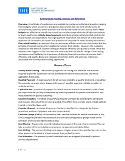
Look at the histogram of the age distribution of
females for the year 2009.
13
> hist(RBCD2009FEMALE$AGE,col="red")
Analysis depends on your imagination and questions you raise …
What did I do with the data?
I started working on the data in collaboration with Dr. Ravi Chinta, Associate
Professor, Xavier University. We cannot handle all episodes (over 8 millions) at
the same time. Right from the beginning we wanted to focus on one medical
condition. We settled for ‘Headache (DRG code = 103)’ and ‘Headache With
Complications (DRG code = 102).’ Isolating the episodes pertaining to these
conditions netted us over 18,381 episodes for the year 2008. This is the segment
14
of data we wanted to study. The first thing we did was to convert the Ascii data
into SPSS files to SAS files to R files.
What is needed to work on such a project?
1. Dexterity with some computing package.
2. A reasonable grounding in sample survey methodology.
Using data from a stratified random sample, one needs to know how to estimate
population parameters and provide confidence intervals. A book by Paul Levy and
Stanley Lemeshow (Sampling of Populations, Wiley 1991) is helpful. The booklet
by HCUP and the website are helpful in explaining how to build national
estimates.
We examined a number of variables and their distributions.
1. Gender
2. Distribution of Gender state by state
3. Distribution of Gender region by region (Northeast; south; Midwest; west)
4. Stratum estimates; national estimates
5. LOS (length of stay)
6. LOS national
7. LOS state by state
8. LOS region by region
9. Average cost per day national
10.Average cost state by state
11.Average cost region by region
12.Who paid?
13.Age national
14.Age state by state
15.Age region by region
16.Headaches versus total nationwide
17.Headaches versus total state by state
18.Headaches versus total region by region
19.Etc.
15
Goal: Estimate the distribution of Gender suffering from headache nationally
Step 1:
Estimate the distribution of Gender stratum by stratum.
Stratum
Male Female
Total Male%
Female%
Weight
1011
3
13
16
18.8%
81.3%
6.54
1012
11
19
30
36.7%
63.3%
6.10
Etc.
Note: The weights are proportional to the size (Total Number of Episodes) of the
strata. These weights are provided by HCUP. When we want to get a national
estimate of the distribution of Gender, we need to calculate the weighted average
of strata distributions.
National estimate
Gender:
Male Female
Percentage: 25.6% 74.4%
Goal: How the distribution of the gender varies from state to state?
Each hospital is identified by the state in which it is located. Pull out all the
episodes that occurred in all hospitals in the state of interest.
State Male Female
Total Male%
Female%
AR
67
177
244
27.5%
72.5%
AZ
130
360
490
26.5%
73.5%
Etc.
A technical note: Recording the data state by state is also stratification. This is
post-stratification. One can use the post-stratified data to get a national estimate
of the distribution of gender suffering from headaches. This is not a problem. The
16
daunting task is to obtain standard errors. The methodology comes under
‘Domain Analysis.’
Here is the bar plot of percentage of women with headache admitted to hospital
state by state and sorted from the lowest to the highest.
VT
UT
RI
CT
OR
OK
KS
NJ
OH
AR
WV
MN
PA
LA
NV
IN
MA
AZ
CA
TN
MI
40
IA
NE
VA
MD
CO
FL
NC
NY
HI
WI
KY
WA
GA
TX
IL
SC
MO
ME
WY
NH
SD
60
0
Percentage
0
Percentage
Women with Headache Admitte
There is some variation in the percentage of women with headache admitted to
hospital, with the least percentage from Vermont at 50% and highest in South
Dakota at 85.7%.
Let us look at regional variations.
Region
Male Female
Total Male%
Female%
Northeast
1071 2932
4003 26.8%
73.2%
Midwest
997
2828
3925 25.4%
74.6%
South
1909 5696
7605 25.1%
74.9%
West
739
2750 26.9%
73.1%
17
2011
Total
4716 13567
18283 25.8%
74.2%
Inter-regional variation is not much.
Goal: Examine the length of stay
1. The length of stay varied from 0 to 62 days. The length is 0 means that the
person was discharged on the same day.
2. The mean length of stay is 2.68 days.
3. The mean length of stay for males is 2.50 days.
4. The mean length of stay for females is 2.75 days.
The distribution of the length of stay in the hospital is given below.
Length TotalFrequency MaleFrequency FemaleFrequency
1
0
738
226
512
2
1
4894
1477
3417
3
2
5274
1365
3909
4
3
3166
729
2437
5
4
1688
382
1308
6
5
1019
213
806
7
6
572
116
456
8
7
330
79
251
9
8
187
39
148
10
9
129
20
109
11
10
84
17
67
12
11
51
12
39
13
12
36
8
28
14
13
28
6
22
15
14
20
9
11
18
16
15
13
0
13
17
16
8
2
6
18
17
11
3
8
19
18
8
2
6
20
19
4
0
4
21
20
2
1
1
22
22
1
1
0
23
23
4
1
3
24
24
1
1
0
25
26
2
1
1
26
27
1
1
0
27
28
1
1
0
28
29
1
0
1
29
30
2
1
1
30
31
2
1
1
31
35
1
0
1
32
36
1
0
1
33
37
1
0
1
34
40
1
1
0
35
48
1
1
0
36
62
1
0
1
The Distribution of the Length of Stay Gender-wise in Percentages
Length
MalePer
FemalePer
1
0
4.79
3.77
2
1
31.32
25.19
19
3
2
28.94
28.81
4
3
15.46
17.96
5
4
8.10
9.64
6
5
4.52
5.94
7
6
2.46
3.36
8
7
1.68
1.85
9
8
0.83
1.09
10
9
0.42
0.80
1.48
1.59
11
10 or more
A bar plot
0 Days
1 Day
2 Days
3 Days
4 Days
5 Days
6 Days
7 Days
8 Days
9 Days
>9 Days
0
5
10
15
20
25
30
Percentage of
People Stayed in Hospitals
Males
Females
Goal: How much each patient was charged?
A column in the data with the heading ‘TOTCHG’ gives total charge levied for each
episode. This is what we did with this column.
20
1. Look at all the episodes in which the patient was discharged on the same
day. Take the average of all charges levied.
2. Look at all the episodes in which the patient stayed for one day. Take the
average of all charges levied.
3. Look at all the episodes in which the patient stayed for two days. Calculate
the charge per day for each patient. Then average.
4. And so on.
The standard deviation of these per day total charges is also calculated. Is it the
best way to convey the cost of staying in a hospital when the ailment is
headache?
No. of Days Total Charge
Stayed
# Episodes
Per Day
Mean $
0
9370
729
1
10565
4831
2
6839
5237
3
5477
3139
4
5076
1695
5
4642
1016
6
4559
568
7
4201
322
8
4199
184
9
4045
129
10
4134
84
21
11
3898
51
12
4027
36
13
3549
28
14
4161
19
15
4172
13
16
4660
8
17
3544
12
18
3696
8
19
4974
4
20
4362
2
22
1824
1
23
5433
4
24
3634
1
26
2897
2
27
4064
1
28
8092
1
29
1455
1
30
6580
2
31
3062
2
35
3803
1
36
6981
1
37
12018
1
22
40
14794
1
48
6018
1
62
951
1
Total
7111
17407
What factors influence these charges?
One strong predictor is the number of co-morbidities each episode entails.
No. of co-morbidities
0
1
2
3
4
5
6
7
8
9
# Episodes Percentage
5577
5371
3829
2131
947
374
104
35
10
3
Total 18381
Gender distribution (percentages)
Year
Females
Males
2005
54
46
2006
55
45
2007
65
35
2008
74
26
2009
73
27
23
30.3
29.2
20.8
11.6
5.2
2.0
0.6
0.2
0.1
0.0
100.0
What’s going on?
Challenging problems
1. Trend analysis
2. Incidence of headaches in relation to total number of admissions – stratum
by stratum – state by state. What is the trend like?
3. When data collection began in 1988 only 8 states participated in the survey.
In 2008, 42 states participated. In 2009, 44 states participated. The size of
the target population is not the same over the years.
4. Integrating two or more data sets.
Elaboration of Idea 4
We have HCUP data.
EPA has PM2.5 Concentration data.
There are more than 1000 monitors around the country monitoring PM2.5
(Particulate Matter 2.5). At each site, how much PM2.5 accumulated is measured 4
times a day every day.
Here is the idea.
Is headache environmental?
Look at an episode → Look up the Zip code
→ Identify all monitors within 6 mile radius of the zip code
→Average PM2.5 concentrations from all the monitors over
the previous ten days from the date of admission
Case -
Headache
Control -
No headache
Choose control well-matched with the case.
24
We have PM2.5 average for both case and control.
Explore.
We focused on ‘headaches.’ What about working on other medical conditions?
How to get the data?
Connection to Biomedical Engineering
I work with the Tissue Engineering Group.
Team
Dr. David Butler
Dr. Jason Shearn
Andrew Breidenbach, Ph.D. student
Andrea Lalley, Ph.D. student
Steve Gilday, Ph.D. student
I also work with the Biomechanics group.
Dr. Jason Shearn
Rebecca Nesbit, Ph.D. student
Nate Bates, Ph.D. student
The tissue engineering group is concerned with musculoskeletal injuries. They
have information on the total number of patients who had injuries of this type for
a year or two. Can we use the HCUP data to fine tune the extent of incidence of
these injuries over the years? Cost? Length of Stay? Gender? Etc.
DRG = 477: Biopsies of Musculoskeletal System and Connective Tissue
DRG = 478
DRG = 479
25
Other data sets
KIDS: Data from pediatric hospitals
SIDS: State-wide Inpatient Discharge data
Emergency data
Introduction to Data Science: Syllabus
Division of Biostatistics and Epidemiology
Department of Environmental Health
College of Medicine
University of Cincinnati
Syllabus
Title:
Introduction to Data Science
Course:
BE 7082
Likely to be offered in Spring, 2015 after Curriculum Committee approval
Introduction
Traditionally, Statistics departments work within the environment of ‘small n –
small p’ data, where n stands for the number of observations and p for the
number of variables. A new discipline ‘Bioinformatics’ arose with the objective of
handling ‘small n – large p’ data. Analyses of gene expression data, protein data,
polymorphism data, etc. come under the purview of ‘Bioinformatics.’ The next
26
step is dealing with ‘large n’ data. This is what ‘Big data’ is made of. A fusion of
Computer Science, Mathematics, and Statistics is needed to handle big data. A
data scientist needs more than the fusion. He should be able to harness the
following, in order of importance, to be a successful data scientist.
1.
2.
3.
4.
5.
Statistics
Mathematics
Computer Science
Machine Learning
Domain Expertise (He/she needs to know the field from which the data
comes from.)
6. Communication and Presentation skills
7. Data visualization
The purported class is intended to provide an introduction to big data. The
students are trained to harness critical skills to become a successful data scientist.
The following is an outline of the contents of the course.
Introduction
1. What is Data Science?
2. Examples
Computing skills
3.
4.
5.
6.
7.
Introduction to R (ff and bigmemory packages)
Python and R
Hadoop and R
MapReduce, Pregel
Cloudera
Machine Learning Tools from Statistics
8. Cluster Analysis
9. Decision Trees and Random Forests
10.Bagging and Boosting
11.Regression
27
12.Logistic Regression
13.Pattern recognition
14.Naïve Bayes
15.Bayesian Networks
16.Outlier Detection
17.Exploratory data analysis
Applications
18.Text mining
19.Social network analysis
20.Designing a spam filter
21.Forecasting in time series
Data visualization
22.Interactive graphs
23.Spatial graphs
24.Trend graphs
Evaluation
1.
2.
3.
4.
Homework – 10 homework sheets –
Project (Presentation is required.)
Mid-term exam Final exam -
Grades
A – 90 and above
B – 80 – 89
C – 70 – 79
D – 60 – 69
F – Below 60
28
30 points
20 points
25 points
25 points
Text book
Rachel Schutt and Cathy O’Neil – Doing Data Science – O’Reilly, Cambridge,
2013.
References
Deborah Nolan and Duncan Temple Lang – XML and Web Technologies for
Data Sciences with R – Springer, New York, 2014.
Nina Zumel and John Mount – Practical Data Science with R – Manning, Shelter
Island, 2014.
Drew Conway and John Myles White – Machine Learning for Hackers –
O’Reilly, Cambridge, 2012.
Yanchang Zhao – R and Data Mining – Academic Press, New York, 2013.
Vignesh Prajapati – Big Data Analytics with R and Hadoop – Packt Publishing,
Mumbai, 2013.
Brett Lantz – Machine Learning with R – Packt Publishing, Mumbai, 2013.
Hadley Wickam – ggplot2 – Elegant Graphs for Data Analysis – Springer, New
York, 2009.
29