US 20070239403A1
(19) United States
(12) Patent Application Publication (10) Pub. No.: US 2007/0239403 A1
Hornbostel
(54)
(43) Pub. Date:
KALMAN FILTER APPROACH TO
Oct. 11, 2007
Related U.S. Application Data
PROCESSING ELECTORMACGNETIC DATA
(60)
(76) Inventor:
Provisional application No. 60/576,201, ?led on Jun.
1, 2004.
Scott Hornbostel, HOUSTON, TX
(US)
Publication Classi?cation
Correspondence Address:
(51)
Int. Cl.
G06F 19/00
(2006.01)
J Paul Plummer
G06F
(2006.01)
Exxon Mobil Upsstream reasch company
(52)
17/40
U.S. Cl. ....................... .. 702/191; 702/189; 702/127;
P.O.B0X 2189
Houston, TX 77252 (US)
702/1; 702/6; 702/190
(57)
ABSTRACT
A method for tracking a sinusoidal electromagnetic signal in
noisy data using a Kalman ?lter or other tracking algorithm.
(21) Appl' NO"
(22) PCT Filed;
11/597,594
API._ 26, 2005
(86)
PCT NO_;
PCT/Us05/14143
§ 371(c)(1),
(2), (4) Date:
Nov. 21, 2006
The method is useful for controlled source electromagnetic
surveying Where longer source-receiver o?csets can cause the
source signal to decay signi?cantly and be di?icult to
retrieve from magnetotelluric or other electromagnetic back
ground
( 41
Initial Estimate of Signal and
Associated Parameters
(42
Project Ahead to the Next Sample
Adjust the New Sample Using the Data
44
No
'
Yes
Patent Application Publication Oct. 11, 2007 Sheet 1 0f 6
Au
US 2007/0239403 A1
9
Ocean
11
u|l||q\
137 MINI?‘
J_/
.||||I||§\
12_\)_
illlillb“
)
"Hill:
Earth
FIG. 1
(Prior Art)
(21
Enter prior estimate Q]; and
its error covariance P]; j
V
(22
253
(23
Project ahead:
Update estimate with
xl;+1 = ¢kxk
‘DI-2+1 = ¢kPk¢I€ + Qk
A measurement zk: A
Xk = xk + Kk(zk ' Hkxk)
Compute error covariance
for updated estimate
L24
FIG. 2
(Prior Art)
Patent Application Publication Oct. 11, 2007 Sheet 2 of 6
US 2007/0239403 A1
(31
PREPARE THE DATA: bandpass filters;
noise editing; resampling; scaling
l
(32
SETUP THE KALMAN FILTER: format
the Kalman eqtns, initialize parameters
V
('33
RUN THE KALMAN FILTER:
(Fiy- 2)
l’
(34
INTERPRET THE RESULTS: displays;
interpretation; inversion for resistivity
FIG. 3
(41
Initial Estimate of Signal and
Associated Parameters
d
(42
Project Ahead to the Next Sample
l
(43
Adjust the New Sample Using the Data
Patent Application Publication Oct. 11, 2007 Sheet 3 0f 6
US 2007/0239403 A1
8642o
$25-: 5.4
a
pm.
4
-8000 -6000 -4000 -2000
0
2000
4000
6000
8000
Time (seconds)
FIG. 5
2.0
$0towu= as<
4970
4980
4990
5000
5010
Time (seconds)
FIG. 6
5020
5030
Patent Application Publication Oct. 11, 2007 Sheet 5 0f 6
US 2007/0239403 A1
235.4
____.__.__]______..__.L___._.____l__..____J._._______L.__.._____
_______J_______J________I_______ _ |_____._____ l_________
|
|
|
“I
-6000
-4000
~2000
0
10-15
-8000
Time (seconds)
FIG. 9
T
000
4000
6000
8000
Patent Application Publication Oct. 11, 2007 Sheet 6 0f 6
US 2007/0239403 A1
5.0
A
4.0 ------
3 5 ------~ -+~~~~
~~a--~-~-——1—
—————+—————
-r-———“---|
4
——————|————————|———————-r———————r~~——~*——1———————+
\l
_|.I_____
I
I
l'_______|_______T_____""_F"_____'_I__“'____T_l_____
l
1.5
~8000
-6000
-4000
-2000
2000
Time (seconds)
FIG. 10
4000
6000
8000
Oct. 11, 2007
US 2007/0239403 A1
KALMAN FILTER APPROACH TO PROCESSING
ELECTORMACGNETIC DATA
[0001] This application claims the bene?t of US. Provi
sional Patent Application No. 60/576,201 ?led on Jun. 1,
2004.
FIELD OF THE INVENTION
Correlations between different detectors could be used to
help separate active-source signals from these noises. Other
signal and noise correlations (e.g., signal correlations on the
tWo horiZontal components) are not optimally used in cur
rent approaches.
[0007] The Kalman ?lter algorithm has its origins in
navigation positioning problems and is particularly suited to
the class of tracking problems (Kalman, 1960). Originally
[0002] This invention relates generally to the ?eld of
geophysical prospecting and, more particularly, to electro
magnetic methods used to explore for hydrocarbons. Spe
ci?cally, the invention is a method for tracking electromag
netic source signals used in controlled source
electromagnetic prospecting so that the signal can be recov
ered from noise.
BACKGROUND OF THE INVENTION
published by Kalman in Trans. of the ASMEiJ. of Basic
Engr, 35-45 (1960), much has been published since on
modi?cations and applications of the basic Kalman ?lter as
summariZed, for example, by BroWn in Introduction to
Random SignalAnalysis and Kalman Filtering, John Wiley
& Sons, NY. (1983). A feW of these modi?cations are of
signi?cance to some embodiments of the current invention.
[0008]
The standard Kalman ?lter runs in one direction
physical surveys use active (man-made) sources to generate
and ?lters data in this direction (or time) sequence. There
fore only previous data in?uences the ?lter result. An
important modi?cation due to Rauch, et al., gives an optimal
electromagnetic ?elds to excite the earth, and deploy
treatment that uses the entire time record: Rauch, “Solutions
receiver instruments on the earth’s surface, the sea?oor, or
inside boreholes to measure the resulting electric and mag
netic ?elds, i.e., the earth’s response to the source excitation.
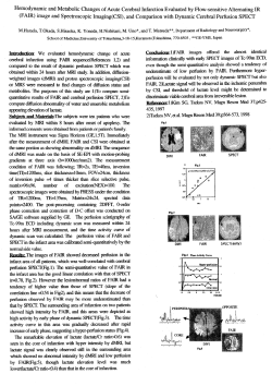
FIG. 1 illustrates the basic elements of an offshore CSEM
survey. A vessel toWs a submerged CSEM transmitter 11
over an area of sub-sea ?oor 13. The electric and magnetic
?elds measured by receivers 12 are then analyZed to deter
to the linear smoothing problem,”IEEE Trans. On Auto.
[0003] Controlled-source electromagnetic (“CSEM”) geo
Control, AC-8, 371 (1963); and Rauch, et al., “Maximum
likelihood estimates of linear dynamic systems,”AIAA J. 3,
1445 (1965). SZelag disclosed another algorithmic modi?
cation that alloWs the ?lter to track sinusoidal signals of a
surface formations) beneath the surface or sea?oor. This
knoWn frequency; see “A short term forecasting algorithm
for trunk demand servicing,”The Bell System Technical
Journal 61, 67-96 (1982). This Was developed to track
annual cycles in telephone trunk load values.
technology has been applied for onshore mineral explora
tion, oceanic tectonic studies, and offshore petroleum and
[0009] FIG. 2 is a ?oW chart illustrating the Kalman
algorithm. Reference may be had to BroWn’s treatise, page
mine the electrical resistivity of the earth structures (sub
mineral resource exploration.
[0004]
Active electromagnetic source signals can be
treated as a sum of sinusoidal signals (e.g., a square-Wave
signal made up of a fundamental frequency With odd har
monics). An example of such a source is the horizontal
electric dipole used in much CSEM Work. As the offset, i.e.,
the distance betWeen such a dipole source 11 and the
receivers 12 increases, the sinusoidal signal can decay
signi?cantly. Moreover, the far o?fsets are often critical for
determining deep resistivity structures of interest. As a
result, a need exists to obtain the best possible signal-to
noise ratio for this sinusoidal signal.
200, for more details.
[0010]
La Scala, et al., disclose use of a knoWn extended
Kalman ?lter for tracking a time-varying frequency.
(“Design of an extended Kalman ?lter frequency tracker,
”IEEE Transactions on Signal Processing 44, No. 3, 739
742 (March, 1996)) The formulation assumes that the signal
remains constant in amplitude. The particular Kalman algo
rithm used is therefore aimed at tracking a signal of
unknoWn frequency Where the frequency may undergo con
siderable change. Lagunas, et al., disclose an extended
WindoWs over Which Fourier analysis or a similar method is
Kalman ?lter to track complex sinusoids in the presence of
noise and frequency changes, such as Doppler shifts. Like
the La Scala method, Lagunas’s algorithm is designed to
track sinusoids of unknoWn frequency. Both methods Will
therefore be sub-optimal if applied to track a signal With
used to calculate the amplitude and phase of selected fre
constant or near constant frequency. Lagunas’s method is
quency component(s). See, for example, Constable and Cox,
“Marine controlled-source electromagnetic sounding 2. The
are relatively small. Neither invention is aimed at processing
[0005] Typical processing methods to improve signal
noise for this EM data involve breaking the data into time
able to also track amplitude changes, provided the changes
PEGASUS Experiment,”Journal of Geophysical Research
electromagnetic survey data obtained using an electromag
101, 5519-5530 (1996). These WindoWs cannot be too large
netic source transmitting knoWn Waveforms at a knoWn
because signal amplitude and relative phase may change
substantially Within the analysis WindoW. Small WindoWs,
hoWever, alloW only minimal signal-to-noise ratio improve
ment. Current methods require a compromise betWeen these
frequency. There is a need for a method for tracking large
amplitude variations and small phase changes about a
knoWn sinusoid, using large WindoWs, or even all, of the
electromagnetic data. The present invention satis?es this
tWo extremes.
need.
[0006] Another problem With existing methods is that they
SUMMARY OF THE INVENTION
don’t take advantage of signal and noise correlations. LoW
frequency magnetotelluric (“MT”) noises, in particular, are
[0011]
a signi?cant problem for active source marine EM imaging
because they can masquerade as signal. (MT noise is elec
tracking amplitude variations and phase changes of a trans
tromagnetic emissions from natural, not active, sources.)
over time by at least one receiver, said signal being trans
In one embodiment, the invention is a method for
mitted periodic electromagnetic signal in noisy data detected
Oct. 11, 2007
US 2007/0239403 A1
mitted at a known frequency, said method comprising the
steps of: (a) selecting a tracking algorithm for tracking a
signal of knoWn frequency; (b) partitioning the detection
related over long time periods because of the sloW rate of
phase change relative to a reference sine Wave. In other
time into intervals Within each of Which the detected signal
Words, information at a particular time gives information
about the signal much later. Fourier analysis on isolated time
and the at least one related parameter are assumed not to
WindoWs, on the other hand, does not use any information
vary; (c) estimating initial values for the detected signal and
outside the current WindoW. In particular, the estimated
the at least one related parameter and assigning these values
amplitudes and phases may be discontinuous betWeen Win
doWs. The Kalman method can also incorporate signal and
to the ?rst time interval; (d) estimating projection of the
initial signal and each related parameter one interval ahead
in time; (e) revising the initial estimates of step (d) using the
data and the tracking algorithm; and (f) repeating steps
(d)-(e) until all data are processed.
[0012]
In some embodiments of the invention, the tracking
algorithm is a Kalman algorithm, involving a state vector
speci?ed by a state equation and a measurement equation. In
noise characteristics such as: noise correlations betWeen
distant detectors (or different components on the same
detector), signal correlations betWeen components, time
varying signal and noise amplitude changes, and predictable
effects of geology on the data.
[0021]
In order to use the Kalman ?lter, the process must
some of those embodiments, the state vector has tWo com
be expressed via tWo linear equations: the state equation and
the measurement equation. In cases that ?t this assumption,
ponents, the signal’s amplitude and the quadrature signal. In
the Kalman algorithm gives the least-squares optimal signal
other embodiments, particularly useful for situations Where
the signal undergoes large amounts of attenuation, the state
estimate With its associated error covariance. The linear
vector has tWo additional components that can be used to
Where it might fail include measurement noise that is not
additive, e.g., some kinds of signal clipping or distortion or
more easily track the signal: the rate of change of the signal
envelope amplitude and the rate of change of the signal’s
relative phase.
assumption Will be valid for most applications. Examples
multiplicative noise. Similarly, the state equation might fail
the linearity assumption if, for example, the signal is totally
unpredictable from one sample to the next or if the system
BRIEF DESCRIPTION OF THE DRAWINGS
[0013] The present invention and its advantages Will be
better understood by referring to the folloWing detailed
description and the attached draWings in Which:
[0014]
FIG. 1 illustrates the ?eld layout for a typical
controlled source electromagnetic survey;
[0015] FIG. 2 is a How chart shoWing the primary steps in
the Kalman algorithm;
[0016] FIG. 3 is a How chart shoWing the primary steps of
one embodiment of the present inventive method using the
Kalman ?lter as the tracking algorithm;
[0017]
FIG. 4 is a How chart of a more general embodi
ment of the present invention; and
[0018] FIGS. 5-10 shoW the results of the present inven
tive method With Kalman algorithm applied to model data
With 0.25 HZ signal frequency and additive random noise.
[0019] The invention Will be described in connection With
its preferred embodiments. HoWever, to the extent that the
folloWing detailed description is speci?c to a particular
embodiment or a particular use of the invention, this is
intended to be illustrative only, and is not to be construed as
limiting the scope of the invention. On the contrary, it is
intended to cover all alternatives, modi?cations and equiva
lents that may be included Within the spirit and scope of the
invention, as de?ned by the appended claims.
DETAILED DESCRIPTION OF THE
PREFERRED EMBODIMENTS
[0020] The present invention is a method of using a
tracking ?lter such as the Kalman algorithm to track sinu
soidal signal and to recover the signal from electromagnetic
noise. The Kalman ?lter approach disclosed herein
addresses the problems With existing approaches discussed
previously. To begin With, a large portion of the data record
can be used to obtain an estimate at each instant. This is
important because electromagnetic data can be highly cor
is nearly unstable Where the siZe of the signal in?uences the
transition matrix. Situations that are mildly nonlinear can
still be modeled using expansions or other approximations
as is done beloW.
[0022]
The required state equation contains a state vector
xk that can be set up in several Ways for electromagnetic data
processing. At a minimum, xk Will contain tWo components.
These are the signal (e.g., horizontal electric ?eld at a
particular location) and its corresponding quadrature signal.
The quadrature is the signal after a 90° phase shift. For
sinusoid signals, the quadrature is proportional to the deriva
tive of the signal. TWo components are required since a
sinusoid is the solution of a second-order differential equa
tion. Additional component pairs Would be needed for each
signal to be estimated at each detector location. Additional
derivatives can also be modeled, if desired, for each esti
mated signal. The additional derivatives are useful since
updates to a derivative give a smoother correction to the
signal estimate.
[0023] The Kalman ?lter requires speci?cation of noise
covariance and signal-drive covariance matrices. The noise
covariance entries Would be used, for example, to indicate
noise level and correlations due to MT noise. The signal
drive covariance entries indicate the required adjustment
rate of the ?lter and any signal correlation betWeen compo
nents.
[0024] After the ?lter parameters are speci?ed, the data
can be preprocessed before beginning the ?lter algorithm. To
begin With, the data can be scaled such that the expected
signal portion of the data has relatively ?at amplitude. In
other Words, the far offsets are scaled up using a rough
prediction of the signal decay rate With offset. The ?lter
algorithm is only required to track changes from this
expected decay rate, Which is more manageable than track
ing the rapid amplitude decay With offset. As these data are
scaled up to balance the signal, the random noise Will be
scaled up as Well. This can be speci?ed in the noise
covariance matrix so that it is built into the algorithm that the
far offset data have more noise.
Oct. 11, 2007
US 2007/0239403 A1
[0025]
In other embodiments of the inventive method,
amplitude problem may be imagined, including doing noth
large changes in amplitude are dealt With by modeling
amplitude decay rates instead of the amplitudes themselves.
ing about the amplitude variation, and all of them are
The decay (or rise) rates may be similar in amplitude even
When the signal itself varies over several orders of magni
[0033] Also in step 31, the expected noise in the noise
tude.
[0026]
covariance matrix (discussed beloW) is preferably speci?ed
so that the algorithm can optimally use various qualities of
Noise bursts or missing data can also be identi?ed
so that the ?lter Will carry a sinusoid through these Zones
Without requiring data. Measurement noise may also be
adjusted to meet the White-noise requirement. These adjust
ments Would include balancing ?lters, DC cut methods,
?lters to remove harmonic noise (if not treated as a signal),
and modeling of colored noise using separate state vari
able(s).
[0027] For a typical square-Wave signal, there are odd
harmonics in addition to the nominal fundamental fre
quency. These harmonics can be ?ltered out (using bandpass
?lters) and processed as separate signals or they can be
modeled simultaneously With the fundamental. Simulta
neous modeling Would make sense if one expected the
harmonic signal adjustments to be correlated With the fun
damental signal adjustments.
[0028] After the model speci?cation and preprocessing,
the Kalman ?lter algorithm can be used to estimate the state
vector components as a function of time and the associated
estimation error bars. This optimal estimate can then be used
in further electromagnetic interpretation by comparing With
parametric models or by using it as an input to an inversion
for resistivity structure as taught by U.S. Pat. No. 6,603,313
to Srnka.
[0029] FIG. 3 shoWs the primary steps in one embodiment
of the present invention. In this embodiment, the Kalman
?lter tracks the amplitude and phase changes of a received
electromagnetic signal as a function of time. In the discus
sion to folloW, the source and/or receiver are assumed to be
moving and thus the source-to-receiver offset is changing as
a function of time (as in FIG. 1 Which depicts a moving
source). The present invention can equally Well be applied to
stationary source and receivers, even though this is not an
ef?cient Way to conduct a CSEM survey.
[0030] Increases in source-to-receiver offset lead to sub
stantial attenuation of the received signal. This is a potential
problem for a tracking algorithm since the expected signal
and corrections to it can vary over several orders of mag
nitude. In step 31 of FIG. 3, certain preliminary steps are
performed to prepare the data measured by the receivers.
One such step deals With the problem of the Wide variation
in the signal over the offset range used in the survey.
[0031]
intended to be Within the scope of the present invention.
There are at least tWo Ways to deal With this
problem. In one approach, the data can be pre-scaled to
compensate for typical amplitude fall-off rates With offset.
Model results covering a range of expected conductivities
should be consulted to determine this amplitude decay. After
scaling, the ?lter task is simpli?ed since one is only tracking
data. For example, there may be random noise bursts (brief
high-amplitude noises). These can be ?agged in preprocess
ing so that the Kalman ?lter can carry the signal sinusoids
through these Zones Without using the data.
[0034] Another desirable preprocessing step involves fre
quency ?ltering to balance the noise spectrum so that the
assumption of White, additive noise is accurate. This may
typically involve scaling doWn the very loW frequency
components (i.e., beloW the fundamental signal frequency)
since ambient MT noise tends to be largest at these frequen
cies. In addition, the data can be loW-pass ?ltered to remove
higher-frequency noises and to alloW resampling to a larger
sample interval. The resampling improves the computational
requirements of the algorithm.
[0035] A typical square-Wave source signal Will include
the odd harmonics in addition to the nominal fundamental
frequency. These harmonics can be ?ltered out (using band
pass or notch ?lters) and processed as separate signals or
they can be modeled simultaneously With the fundamental.
Simultaneous modeling may be preferred if one expects the
harmonic signal adjustments to be correlated With the fun
damental signal adjustments.
[0036] In summary of step 31, several data preparation
techniques including those described above are used in
preferred embodiments of the invention, but none of them
are critical to the invention.
[0037] In step 32 of FIG. 3, the Kalman ?lter is set up for
the application. In other embodiments of the invention,
tracking algorithms other than the Kalman ?lter may be
used. FIG. 4 shoWs the basic steps that are performed by
such a more generic embodiment of the invention. In step
41, initial estimates of the signal and associated parameters
are input to the algorithm. Typically, these initial time
sample values Would include the signal of interest and its
derivative. These initial values may be determined from
near-offset data With high signal-to-noise ratio. Altema
tively, an arbitrary initial guess may be used under the
assumption that the algorithm Will quickly converge on
correct values. In step 42, these are projected ahead one
sample using, for example, the rotation matrix discussed
beloW in connection With the Kalman ?lter. In step 43, the
neW sample is adjusted based on the measured data and the
speci?cs of the particular tracking algorithm. Step 44 con
cludes one cycle of the loop, Which is repeated until the data
is exhausted, i.e., until the signal has been projected ahead
for the time period for Which data Were collected. This
explanation is brief because further details that folloW in
connection With the Kalman ?lter Will also apply to the
variations from this baseline case and the siZe of the cor
generic algorithm.
rections is relatively constant.
[0038]
[0032] In an alternate approach to the amplitude variation
issue, state variables that correspond to amplitude and phase
rates of change are added. These rates are easier to model
since they are relatively constant in value for amplitudes that
are decaying or rising exponentially. Other approaches to the
The Kalman ?lter is the preferred solution for a
state-space formulation of the electromagnetic signal-track
ing problem. This formulation has tWo matrix equations: the
“state” equation and the “measurement” equation. The state
equation is
Oct. 11, 2007
US 2007/0239403 A1
Where xk is the state vector at sample k, (I)k is the state
transition matrix, and Wk is the state forcing function. The
time scale is partitioned into ?nite intervals, and the mea
surement by each receiver is converted to a single number
(called Zk in the measurement equation beloW) for each time
interval. Data sample k refers to the digitized output for the
kth time interval, Where k is an integer index denoting
sequential time intervals. The forcing function is a White
sequence that represents differences in the next state vector
sample from What Would otherWise be predicted by the
transition matrix applied to the current sample. The transi
tion matrix gives the predicted state vector at the next
sample in the absence of any innovation (Where Wk is Zero).
SZelag’s method Was adapted to model an oscillating signal.
SZelag used a tWo-element state vector With components for
(1+T-AA) in going to the next sample. This Will occur to the
signal envelope if both xS and xq are scaled by this factor:
xq(k+1)=(1+T-AA)-(—S-xS(k)+C-xq(k)).
(6)
Next, consideration is given to a small relative phase change
occurring at a rate of v radians/ sec. This Would cause a phase
shift of vT When going to the next sample. This can be
incorporated in the state equation by modifying the rotation
sinusoids of equations (5) as folloWs:
C=cos(2nfT+vT), and
§=sin(2nfT+vT).
the oscillating signal and its quadrature signal (proportional
C=cos ZnfT-vT sin ZnfT, and
to the derivative). Additional components can be used to
§=sin 2nfT+vT cos Zn?".
model further derivatives of the signal in other embodiments
of the invention. For the tWo-component case, the transition
matrix that Would produce an oscillation at frequency f is
(7)
In order to lineariZe this, use is made of the fact that vT<<l
to reWrite Eq. (7) as:
(8)
Combining equations (6) and (8) and keeping only ?rst
order corrections yields the modi?ed state equation:
given by
and
Where f is the signal frequency and T is the sample interval.
[0039] In a preferred embodiment of the invention, this
simple formulation is expanded to instead track the ampli
tude and relative phase, since amplitude and relative phase
Will change gradually With time (offset) for the typical
CSEM problem. This formulation uses a four-component
state vector:
Where xS is the oscillating signal, xq is the quadrature signal,
AA is the rate of change of the amplitude of the signal’s
envelope, and v is the rate of change of the signal’s relative
phase (i.e, the frequency shift). Since the amplitude and
phase are not linearly related to the signal, a small-correction
lineariZation of the state equation is implemented in one
embodiment of the invention. Because variations in v and
AA are expected be small, the linear assumption can be
expected to be valid.
[0040] This lineariZation process is begun by estimating
the values of xS and xq for sample (k+l) given the values at
sample k for the four elements of the state vector. If there are
no changes in amplitude or relative phase, the simple
rotation matrix (I) of Equation (2) gives the projected values
of xS and xq at the next sample:
It may be noted that changes from a constant amplitude
sinusoid occur only through the AA and v elements since
only at these elements is Wk nonZero.
[0041] The covariance matrix associated With Wk also
must be speci?ed. This is the means for controlling the
adaptation rate of the ?lterilarge covariance in Wk means
that larger changes in AA and v are required. When several
data components are being modeled, signal correlations can
be indicated by the off-diagonal elements in the state cova
riance matrix.
[0042] Other modi?cations to the state equation are also
possible. At a minimum, xk Will contain tWo components.
These Would be the signal (e.g., horiZontal electric ?eld at a
particular location) and its corresponding quadrature signal
(proportional to the derivative). TWo additional components
are used above to model amplitude and phase changes.
Additional components Would be needed for each signal to
be estimated at each detector location. Additional deriva
tives can also be modeled, if desired, for each estimated
signal. The additional derivatives may be useful since
updates to a derivative give a smoother correction to the
signal estimate.
[0043] The measurement equation for the Kalman ?lter in
the above-described embodiment is given by
Zk=Hkxk+vk
In this embodiment of the invention, it is next assumed that
the amplitude (signal envelope) increases at a rate of AA per
second. In other Words, the amplitude is multiplied by
(11)
Where Zk is the measured data at sample k, H=[l 0 0 0]‘ is the
measurement matrix that selects xS in the state vector, and vk
is the measurement noise. The Kalman algorithm Works Well
Oct. 11, 2007
US 2007/0239403 A1
for noise that is White, or approximately White. If the noise
is narrow band, e.g., sinusoidal, it can be modeled as a
separate signal component and removed. The associated
covariance matrix for vk gives the expected noise variance
the least-squares solution for that sample is determined at
that time by straightforWard evaluation of the equations in
Particularly noisy Zones could also be speci?ed With larger
the solution process. The state and measurement equations
specify hoW the state of the system progresses and hoW the
measurements relate to the state of the system. The covari
ance matrices Qk and Rk in FIG. 2 correspond to the
quantities Wk and rk in the state and measurement equations.
The values for Qk are typically determined by trial and error;
variances to minimize effects from noise bursts. The cova
they determine hoW quickly the ?lter reacts to changes in the
and correlation. The variance can be time-varying as it
Would be When Working With scaled data (i.e., the noise
Would change exponentially for exponentially scaled data).
riance matrix for vk is also the place Where one Would
include information on correlated noise for the multiple
component case. This Would be helpful, for example, When
a distant detector contains information on MT noise.
[0044] In concluding the discussion of step 32 of FIG. 3,
it can be seen that the Kalman ?lter approach disclosed
herein addresses the problems noted above in the Back
ground section. To begin With, a large effective data WindoW
can be used to obtain an estimate at each instant. This is
important because electromagnetic data can be highly cor
related over long time periods because of the sloW rate of
phase change relative to a reference sine Wave. In other
Words, information at a particular time gives information
about the signal much later. Fourier analysis on isolated time
WindoWs, on the other hand, does not use any information
data. The values of Rk are determined from the noise
variance (expected value of the square of the noise) and
covariance (correlations betWeen noise components, if nec
essary). In addition to the least-squares best solution for the
state vector xk, the Kalman algorithm also gives the related
error covariance for this solution. Of course, the optimal
nature of such a solution depends on the accurate speci?
cation of the state equation and the measurement equation,
including the required covariance matrices for the state and
measurement noises.
[0048]
The optimal estimate of the state vector can be used
in several Ways during the interpretation phase (Step 34 of
FIG. 3). For example, the signal estimate xS can be compared
With parametric models to select among several modeled
resistivity structures. Altemately, xS can be used as an input
outside the current WindoW. In particular, the estimated
to an inversion for resistivity structure. AA and v could also
amplitudes and phases may be discontinuous betWeen Win
doWs. The Kalman method can also incorporate signal and
be used instead of xS in either parametric studies or inver
noise characteristics such as the folloWing: noise correla
tions betWeen distant detectors (or different components on
the same detector), signal correlations betWeen components,
time-varying signal and noise amplitude changes, and pre
dictable effects of geology on the data.
[0045]
s1on.
[0049] Another interpretation approach is the use of AA
and v in a “fast” 1D or 2D inversion. In one such embodi
ment, these state-vector elements are blocked to give piece
Wise exponential amplitude functions that Would correspond
With individual layers in a simpli?ed geology.
In step 33 of FIG. 3, the state equation, measure
ment equation, and associated covariance matrices are used
to apply the Kalman ?lter in the manner indicated in FIG. 2.
The Kalman ?lter normally runs in one direction. There are
at least tWo Ways to use information ahead of the current
sample, i.e., data measured later in time. One option is to
start part-Way into the data and run backwards to get an
initial estimate for the forWard run. Another option is to
employ the previously mentioned ?lter modi?cations of
Rauch, et al., that include all the data ahead of the current
sample. The Rauch approach has problems With the modi
?ed state equation (9) and (10) because of the data depen
dence of the transition matrix (I).
EXAMPLE
[0050] An example With modeled horiZontal electric
dipole data is illustrated in FIGS. 5 to 10. FIG. 5 shoWs the
modeled data With additive random noise. The signal fre
quency is 0.25 HZ and decays roughly exponentially aWay
from the Zero -time position. The additive noise is taken from
recorded ambient magnetotelluric noise. FIG. 6 illustrates a
bloW-up of this noisy input data (initial signal plus additive
noise) 61 at around 5000 seconds. Plotted on the same ?gure
is the noise-free signal portion 62 of the model data and an
estimate 63 of the signal made by using the method of the
present invention. The estimate 63 is nearly equal to the
noise-free signal 62, and dif?cult to distinguish from it in
[0046] The output from the Kalman ?lter Will be the
optimal (minimum mean-square error) state vector values
and the associated signal error covariance matrices (error
bars). A different tracking algorithm might use a different
FIG. 6. This close similarity is a measure of the present
inventive method’s success, because the method does not
error minimiZation criterion.
ment of the present invention that Was used in this example
[0047] FIG. 2 may be referred to again for a summary of
hoW the Kalman ?lter Works in the present inventive
method. At step 21, initial values are estimated for the state
vector and its covariance at some time sample. At step 22,
otherWise is the one described above as preferred. The offset
“knoW” the model signal. It is given only the noisy data as
input but is able to recover the signal portion. The embodi
employs the Kalman ?lter as the tracking algorithm, and
the Kalman algorithm calculates the Kalman gain Kk by
evaluating the equation shoWn. The Kalman gain speci?es
hoW to modify the measured data in order to best merge it
With the guess of the state vector. This merging of data is
performed in step 23. At step 24, the error covariance for the
neW estimate is evaluated. Finally, in step 25, the neW
estimate is used to project ahead in time to the next sample,
and the process is repeated. When each sample is processed,
that corresponds to the portion represented in FIG. 6 is
approximately 4000 m.
[0051] FIG. 7 shoWs the amplitude rate of change AA of
the noise-free signal (solid line 71) and the estimated value
of AA (jagged line 72) obtained by the Kalman ?lter using
the noisy data. It may be noted that the quality of this
estimate is best in the central portions of the data Where the
signal strength is largest.
[0052]
FIG. 8 shoWs the rate of relative phase change v of
the noise-free signal (solid line 81) and the estimated value
Oct. 11, 2007
US 2007/0239403 A1
of V (jagged line 82) obtained by the Kalman ?lter using the
noisy data. Again, the quality of this estimate is best in the
central portions of the data Where the signal strength is
largest.
[0053] FIG. 9 illustrates the signal amplitude of the noise
free input data (solid curve 91) compared With the Kalman
estimate (dashed curve 92). The semilog plot shoWs the
more than three orders of magnitude change in the signal
strength. FIG. 10 shoWs a similar relative phase comparison
of input signal 101 versus Kalman estimate 102.
[0054] The foregoing description is directed to particular
embodiments
illustrating it.
the art, that
embodiments
of the present invention for the purpose of
It Will be apparent, hoWever, to one skilled in
many modi?cations and variations to the
described herein are possible. All such modi
6. The method of claim 1, further comprising an initial
data scaling step.
7. The method of claim 1, Wherein the transmitted signal
is a Fourier component of a source signal in an electromag
netic survey of a subsurface formation.
8. The method of claim 7, comprising a ?nal step of
determining the subsurface formation’s resistivity structure
from the estimates of the signal or the at least one related
parameters.
9. The method of claim 2, Wherein a small correction
lineariZation is implemented in the state equation.
10. The method of claim 2, Wherein an estimate of the
signal and its associated error is obtained for every time
interval.
11. The method of claim 4, Wherein the Kalman algorithm
is modi?ed to alloW the addition of AA (the time rate of
?cations and variations are intended to be Within the scope
change of the signal’s envelope amplitude), and v (the time
of the present invention, as de?ned by the appended claims.
rate of change of the signal’s relative phase) to the state
vector, by using a small correction lineariZation assumption,
We claim:
1. A method for tracking amplitude variations and phase
changes of a transmitted periodic electromagnetic signal in
noisy data detected over time by at least one receiver, said
signal being transmitted at a knoWn frequency, said method
comprising the steps of:
(a) selecting a tracking algorithm for tracking a signal of
knoWn frequency;
(b) estimating initial values for the detected signal and at
least one related parameter;
(c) partitioning the detection time into intervals Within
each of Which the detected signal and the at least one
related parameter are assumed not to vary and assign
ing the estimated initial values to the ?rst time interval;
(d) estimating projection of the initial signal and each
related parameter one interval ahead in time;
said lineariZation assumption comprising: (i) the amplitude
of the signal envelope is assumed to be multiplied by
(1+T-AA) Where AA is the time rate of change of the signal
envelope’s amplitude and T is the interval time, and (ii) the
signal is assumed to undergo a phase shift of vT Where v is
the rate of change of the signal’s relative phase, and vT is
assumed to be <<l.
12. A method for producing hydrocarbons from a subsur
face region, comprising:
(i) performing a controlled-source electromagnetic survey
of the subsurface region:
(ii) obtaining results of the survey Wherein signal is
retrieved from background noise in data recorded by a
detector by a method comprising:
(a) selecting a tracking algorithm for tracking a signal
of knoWn frequency;
(e) revising the initial estimates of step (d) using the data
and the tracking algorithm;
(b) estimating initial values for the detected signal and
(f) repeating steps (d)-(e) until all data are processed.
2. The method of claim 1, Wherein the tracking algorithm
(c) partitioning the detection time into intervals Within
is a Kalman algorithm involving a state vector speci?ed by
related parameter are assumed not to vary and
at least one related parameter;
each of Which the detected signal and the at least one
a state equation and a measurement equation, said state
assigning the estimated initial values to the ?rst time
vector having at least the folloWing tWo components: the
detected signal’s amplitude and said at least one selected
related parameter.
interval;
3. The method of claim 2, Wherein the state vector has tWo
components and said at least one related parameter is
proportional to the time derivative of the signal (the quadra
ture signal).
(d) estimating projection of the initial signal and each
related parameter one interval ahead in time;
(e) revising the initial estimates of step (d) using the
data and the tracking algorithm;
4. The method of claim 2, Wherein the state vector has
(f) repeating steps (d)-(e) until all data are processed.
four components: the signal’s amplitude; the quadrature
signal amplitude; the time rate of change of the signal’s
(iii) drilling a Well into a layer in the subsurface region
envelope amplitude; and the time rate of change of the
signal’s relative phase, said latter tWo components being
used to track a signal experiencing substantial attenuation.
5. The method of claim 2, Wherein the Kalman algorithm
is adapted to use data detected later in time in the revising
step.
identi?ed as a possible hydrocarbon reservoir from
resistivity determinations based on the detected elec
tromagnetic signal; and
(iv) producing hydrocarbons from the Well.
*
*
*
*
*