1. science
2. mathematics
3. arithmetic

MIDTERM REVIEW AND SAMPLE EXAM
Abstract. These notes outline the material for the upcoming exam.
Note that the review is divided into the two main topics we have covered
thus far, namely, ordinary differential equations and linear algebra with
applications to solving linear systems
Contents
1. Ordinary Differential Equations.
1.1. Reduction to a first-order system.
1.2. First-order systems of ODEs: existence and uniqueness theory.
1.3. Autonomous first-order systems: critical points, linearization,
and stability analysis.
1.4. Solving ODEs: analytic methods (and numerical methods to
be covered later)
2. Linear Algebra
2.1. Vectors and Matrices
2.2. Vector Spaces
2.3. Linear systems of equations.
3. Midterm Sample Exam
1
2
4
8
12
15
15
17
20
23
1. Ordinary Differential Equations.
An nth-order ordinary differential equation in implicit form reads
(1)
F (t, y, y 0 , ..., y (n) ) = 0,
F : Ωt × Ω → Rm ,
where y ∈ Rm , Ωt ⊆ R, Ω ⊆ Rm×(n+1) . Componentwise, the ODE
system can be written as

  
F1 (t, y, y 0 , ... , y (n) )
0
 F2 (t, y, y 0 , ... , y (n) )  0

  
 =  ..  .

..

 .
.
Fm (t, y, y 0 , ... , y (n) )
Date: Today is October 18, 2012.
1
0
2
MIDTERM REVIEW AND SAMPLE EXAM
Equivalently, in explicit form the system y (n) = f (t, y, y 0 , ..., y (n−1) ) can be
written in its component form as
 (n)  

y1
f1 (t, y, y 0 , ... , y (n−1) )
 (n)  
y2   f2 (t, y, y 0 , ... , y (n−1) ) 

 . =
(2)

..
 .  

.
 . 
fm (t, y, y 0 , ... , y (n−1) )
(n)
ym
where now f : Ωt × Ω → Rm with y ∈ Rm , Ωt ⊆ R,
example, take m = n = 2, then
00 y1
f1 (t, y1 , y2 , y10 , y20 )
=
.
00
f2 (t, y1 , y2 , y10 , y20 )
y2
Ω ⊆ Rm×n . As an
Definition 1.1 (Solutions of ODEs). The solution of a system of ODEs (2)
is a function u ∈ Rm such that
u(n) = f (t, u, u0 , ..., u(n−1) ).
Remark 1.2 (Initial conditions). Generally, the solution of the system (2)
admits infinitely many solutions, depending on the initial conditions. To
obtain a unique solution, the initial conditions must be specified.
Definition 1.3 (Initial Value Problem). An initial value problem (IVP) is
a system of ODEs (2) together with appropriate initial conditions,
y (i) (t0 ) = ci ∈ Rm ,
i = 1, ..., n − 1.
1.1. Reduction to a first-order system. Here, we show that general
nth-order systems of ODEs are equivalent to first-oder systems of larger
dimension. This, in turn, implies that we can work with first order systems
almost exclusively in analyzing and solving general nonlinear problems.
An nth-order system of ODEs (2) can be written as a first-order nonlinear
system as follows. Let z1 = y and zi := z (i−1) , i = 2, ..., n. Then, the
equivalent first-order system is
z10 = z2
z20 = z3
..
.
0
zn−1 = zn
zn0 = f (t, z1 , ..., zn ).
Note that zi ∈ Rm for i = 1, ..., n. If we write the components of zi as zij ,
j = 1, , , ., m, then we can write the first-order system for z in terms of its
m × n components as follows:
0
zij
= zi+1,j ,
0
znj
= fj (t, z11 , ..., z1m , ..., zn1 , .., znm ),
i = 1, ..., n,
j = 1, ..., m,
j = 1, .., m.
MIDTERM REVIEW AND SAMPLE EXAM
3
Example 1.4. Take n = 2 and m = 1, then we have the scalar second-order
equation
y 00 = f (t, y, y 0 ),
f : Ωt × Ω → R,
Ω ⊂ R.
Note that, if we set f (t, y, y 0 ) = − mk1 y, then we have the equation of a
mass-spring system
m1 y 00 + ky = 0.
To write the equation as a first order system, we set z1 = y and z2 = z10 = y 0
such that z20 = y 00 and the second order ODE becomes
z10 = z2
z20 = f (t, z1 , z2 ) = −
k
z1 .
m1
Thus, we have the equivalent linear first-order system
0
1
z
y
0
z = Az, A =
, z= 1 =
.
k
− m1 0
z2
y0
Example 1.5. Take n = m = 2. Then, as mentioned above, we have a
system of two second-order ODEs
00 y1
f1 (t, y1 , y2 , y10 , y20 )
=
.
00
f2 (t, y1 , y2 , y10 , y20 )
y2
We thus let z11 = y1 , z12 = y2 , z21 = y10 , and z22 = y20 and arrive at the
first-order system
0
z11
0
z12
0
z21
0
z22
=
=
=
=
z21 ,
z22 ,
f1 (t, z11 , z12 , z21 , z22 ),
f2 (t, z11 , z12 , z21 , z22 ).
An example of such a system is given by the mass spring system of ODEs
from the homework:
m1 y100 = −k1 y1 + k2 (y2 − y1 ),
m2 y200 = −k2 (y2 − y1 ),
or
k2
k1
y1 +
(y2 − y1 ),
m1
m1
k2
= −
(y2 − y1 ).
m2
y100 = −
y200
4
MIDTERM REVIEW AND SAMPLE EXAM
If we let m1 = m2 = 1, k1 = 3, and k2 = 2 we have
y100 = −5y1 + 2y2 ,
y200 = 2y1 − 2y2 ,
giving
f1 (t, y1 , y2 , y10 , y20 ) = −5y1 + 2y2 ,
f2 (t, y1 , y2 , y10 , y20 ) = 2y1 − 2y2 .
Thus, the first-order system of ODEs for z becomes
0
z11
0
z12
0
z21
0
z22
=
=
=
=
z21 ,
z22 ,
−5z11 + 2z12 ,
2z11 − 2z12 .
Remark 1.6 (Reduction to first-order system). To summarize, we have
shown that in general an nth-order system of ODEs is equivalent to a firstoder system of larger dimension. This, in turn, implies that we can work
with first order systems almost exclusively in analyzing and solving ODEs.1
While in general we are only able to solve a small class of first-order
systems analytically, numerical methods have been developed for a variety
of first-order systems and provide tools for treating more general nonlinear
problems.
1.2. First-order systems of ODEs: existence and uniqueness theory. Before reviewing various solution techniques, we give some definitions
and state a general existence and uniqueness result for first-order systems
of ODEs. We begin with the local existence and uniqueness result.
Theorem 1.7 (Local Existence and Uniqueness). Consider a first-order
IVP
 0 

y1
f1 (t, y1 , ..., yn )
 ..  

..
.=
 , y(t0 ) = y0 .
.
0
fn (t, y1 , ..., yn )
yn
Assume that fi (), i = 1, ..., n, are continuous functions with continuous
∂fi
(), i, j = 1, ..., n, in some domain Ωt × Ω such that
partial derivatives ∂y
j
(t0 , y0 ) ∈ Ωt × Ω, where Ωt ⊆ R and Ω ⊆ Rn . Then, their exists a unique
solution to the IVP for t0 − α < t < t0 + α, where α > 0.
1We note that in some special cases, (e.g., second-order ODEs) it is preferable to work
directly with the given equation. As we have seen in the homework (see also the sample
exam) the solution to second-order linear systems with constant coefficients can be found
by substituting
y = xeωt
into the system of ODEs, which then reduces solving the system to solving an eigenvalue
problem.
MIDTERM REVIEW AND SAMPLE EXAM
5
Note that the result of the theorem is referred to as a local result since it
only holds in some neighborhood about t0 .
Example 1.8. Consider the first-order IVP
y 0 = f (t, y),
y(t0 ) = y0 .
Then, we have the following three possibilities:
∂f
• The IVP has a unique solution near (t0 , y0 ) if f and ∂f
∂t , and ∂y are
continuous near (t0 , y0 ). As an example, consider the equation
y0 = y2,
y0 = 1,
1
which has the unique solution y = − t−1
for t < 1, but blows up as
t → 1.
• The IVP has a solution but it is not unique if only f is continu∂f
ous near (t0 , y0 ) and not ∂f
∂t , and ∂y . As an example, consider the
equation
√
y 0 = y, y0 = 0,
which has the solutions y = 0 and y = 14 t2 .
• The IVP does not have a solution. As an example, consider the
equation
|y 0 | + |y| = 0, y(0) = c.
1.2.1. Linear first-order systems of ODEs. Linear first-order systems are
an important class of ODEs since they are well understood theoretically.
Moreover, the established techniques that have been developed for first-order
linear problems can be used to analyze and solve more general nonlinear and
higher-order problems.
Definition 1.9 (Linear ODE systems). A first-order system of ODEs is
linear if it can be written as
y 0 = A(t)y + g(t),
where
aij = aij (t).
Equivalently, we can write this system as
y10 = a11 (t)y1 + ... + a1n (t)yn + g1 (t)
..
.
0
yn = an1 (t)y1 + ... + ann (t)yn + gn (t)
Recall that, the system is homogenous if g(t) = 0.
Definition 1.10 (General Solution of nonhomogenous problem). The general solution to a nonhomogenous system of linear ODEs is
y = y (h) + y (p) ,
where y (h) is a solution to the homogenous problem and y (p) is any solution
to the nonhomogenous problem.
6
MIDTERM REVIEW AND SAMPLE EXAM
Remark 1.11 (Principle of Superposition). The set of all solutions to the
homogenous system,
y 0 − Ay = 0,
forms a vector space, which yields the so-called principle of superposition.
That is, (1) y = 0 is a solution to the homogenous system and (2) if y (1) , y (2)
are solutions to the homogenous system, then
(αy (1) + βy (2) )0 − A(αy (1) + βy (2) ) = α((y (1) )0 − Ay (1) ) + β((y (2) )0 − Ay (2) )
= α0 + β0 = 0,
where α, β ∈ R are arbitrary constants. Thus, applying this result n − 1
times gives the principle of superposition: if y (1) , ..., y (n) are solutions to the
linear homogenous system, then so is
y = c1 y (1) + c2 y (2) + ... + cn y (n) ,
where c1 , ..., cn are arbitrary constants.
Definition 1.12 (General Solution of homogenous problem). The general
solution to a homogenous system of linear ODEs is
y = c1 y (1) + c2 y (2) + ... + cn y (n) ,
where y (1) , ..., y (n) form a basis (fundamental solution set) of the system.
Definition 1.13 (Linear independence). The solutions (functions of t) y (1) , ..., y (n)
are linearly independent if and only if
 (1)

(2)
(n)
y1 (t) y1 (t) . . . y1 (t)
 (1)

y2 (t) y2(2) (t) . . . y2(n) (t)

 6= 0,
W (t) = det  .

 ..

(1)
(2)
(n)
yn (t) yn (t) . . . yn (t)
for some t ∈ I.
Example 1.14. For a 2 × 2 system
(1)
(2)
y (t) y1 (t)
W (t) = det 1(1)
(2)
y2 (t) y2 (t)
!
which is the same as the Wronskian for a second-order linear ODE since,
as seen in Example 1.4, this equation can be reduced to a 2 × 2 system. This
follows since the solutions to the 2 × 2 system are y (1) = y and y (2) = y 0 .
Remark 1.15. Given the superposition principle for homogenous problems,
it follows that y = y (h) + y (p) satisfies the nonhomogenous problem:
(y (h) + y (p) )0 − A(y (h) + y (p) ) = y (h) − Ay (h) + y (p) − Ay (p) = 0 + g.
MIDTERM REVIEW AND SAMPLE EXAM
7
Remark 1.16 (Existence and Uniqueness: Linear ODE Systems). The existence and uniqueness theorem simplifies in the case of a first-order linear
system of ODEs. Here we note that
∂fi
= aij (t),
∂yj
i, j = 1, ..., n.
The theorem thus reduces to the following result.
Theorem 1.17. Let aij (t), i, j = 1, ..., n, be continuous functions of t on
some interval I = (α, β), with t0 ∈ I. Then there exists a unique solution
to the IVP on the interval I.
Example 1.18. Consider the scalar fist-order linear IVP:
y 0 + p(t)y = q(t),
y(t0 ) = c0 .
By the theorem, if p(t) and q(t) are continuous on an interval I containing
t0 , then, there exists a unique solution to the IVP on I.
Example 1.19. Consider the scalar second-order linear IVP:
y 00 + p(t)y 0 + q(t)y = g(t),
y(t0 ) = c1 , y( t0 )0 = c2 .
This problem can be reduced to a first-order system and thus by the theorem,
if p(t), q(t), and g(t) are continuous on an interval I containing t0 , then,
there exists a unique solution to the IVP on I.
Remark 1.20 (Linear ODE). There are various interpretations of the equation
y 0 + p(t)y = q(t), y(t0 ) = y0
that lead to some additional useful insights:
• Physically, we can interpret the equation as prescribing the velocity
of a point particle moving on a line in time, t.
• Geometrically, we can interpret the equation as specifying the slope
of the graph of a function y(t). It the slope is plotted pointwise as a
vector field (direction field), then the solution curves must be tangent
to the direction field. Note that the slope is constant along curves
f (t, y) = c, called the isoclines.
• We can write the solution to the equation explicitly as:
y = y (h) + y (p) ,
where y (h) solves the homogenous problem
y 0 + p(t)y = 0
and y (p) is any solution to the nonhomogenous problem
y 0 + p(t)y = q(t).
8
MIDTERM REVIEW AND SAMPLE EXAM
This follows because the equation is linear:
y 0 + p(t)y = (y (h) + y (p) )0 + p(t)(y (h) + y (p) )
= (y (h) )0 + p(t)y (h) + (y (p) )0 + p(t)y (p)
= 0 + q(t).
We solve the homogenous problem using separation of variables, which
has the general solution
y (h) (t) = ce
R
−p(t)dt
.
To find a particular solution
R of the nonhomogenous equation we use
an integrating factor µ = e −p(t) and obtain
Z R
(p)
y = e p(t) q(t)dt.
Thus, the general solution of the nonhomogenous problem is
Z R
R
(h)
(p)
−p(t)dt
y = y + y = ce
+ e p(t) q(t)dt.
1.3. Autonomous first-order systems: critical points, linearization,
and stability analysis. An autonomous first-order system of nonlinear
ODEs can be linearized using Taylor expansion and under appropriate assumptions the type and stability of the critical points of the nonlinear system
can be analyzed using the resulting linear system. The following discussion
summarizes this result.
Definition 1.21 (Autonomous first-order system). An autonomous nonlinear first-order system is given by y 0 = f (y), where the right hand side f does
not depend explicitly on t.
1.3.1. Critical points via the Phase Plane method and linearization.
Definition 1.22 (Critical points). The critical points, yc , of the autonomous
nonlinear system y 0 = f (y) are points for which f is undefined or that satisfy
f (yc ) = 0.
As shown in the sample exam, we can assume that yc = 0. Applying
Taylor expansion near the critical point we have


∂f1
∂f1 ···
 ∂y1
∂yn 

 .
.
.


..
..  .
f (y) = f (0) + Jf (0)(y − 0) + H.O.T., Jf (0) =  ..
 ∂fn
∂fn 
···
∂y1
∂yn 0
Now, since f (0) = 0, if we let A = Jf (0) and let h(y) = H.O.T., then we
can write the autonomous system as
y 0 = f (y) = Ay + h(y).
MIDTERM REVIEW AND SAMPLE EXAM
9
If we drop the function h(y) we obtain the linearized system such that near
the origin y 0 ≈ Ay. We have the following result concerning the use of this
approximation.
Theorem 1.23 (Linearization). Consider the autonomous first-order system y 0 = f (y). If fi , i = 1, ..., n, are continuous and have continuous partial
derivatives in a neighborhood of the critical point, yc , and det A 6= 0, then the
kind and stability of the critical points of the nonlinear system are the same
as the system y 0 = Ay obtained by linearization. We note that exceptions
occur when the eigenvalues of A are purely imaginary.
This result requires analysis of the critical points of the linearized system
y 0 = Ay, which we review next for n = 2. We note that similar analysis can
be conducted for general n × n systems.
Remark 1.24. We note that in our analysis we use the Phase Plane method,
in which we consider the components of the solution y1 (t) and y2 (t) as defining parametric curves in the y1 y2 -plane (the phase plane). If we plot all such
trajectories for a given ODE system, then we obtain the phase portrait. Note
that y1 = y2 = 0 is a critical point of the system since the slope of the trajectory at the critical point is undefined:
dy2
y0
a21 y1 + a22 y2
0
= 20 =
= .
dy1
y1
a11 y1 + a12 y2
0
1.3.2. Classification of critical points. To determine the type of each critical
point we compute the eigenpairs (λ, x) of A to find the general solution to
the homogenous system y 0 = Ay and then study the behavior as t → ±∞.
There are a total of 4 cases to consider. Examples of finding the solution to
such systems for the case of a center and saddle point are provided in the
sample exam.
(1) Node: λ1 , λ2 ∈ R and λ1 λ2 > 0. We call the node proper if all the
trajectoreis have a distinct tangent at the origin. In this case we have
λ1 = λ2 . The node is improper if all trajectories have same tangent
at the origin, except for two of them. In this case, λ1 6= λ2 . The
node is degenerate if A has only a single eigenvector. In this case,
we solve for the first eigenvector x and then solve for the generalized
eigenvector u, by solving the system (A − λI)u = x. Note that,
the eigenvectors are linearly independent provided A is symmetric
or skew symmetric.
(2) Saddle point: λ1 , λ2 ∈ R and λ1 λ2 < 0. In this case, we have two
incoming and two outgoing trajectories, all others miss the origin.
(3) Center: λ1 , λ2 ∈ C and λ1 = iµ, λ2 = −iµ. The trajectories are
closed around the origin.
(4) Spiral: λ1 , λ2 ∈ C and real(λi ) 6= 0, i = 1, 2. Here the trajectories
spiral to or from the origin.
10
MIDTERM REVIEW AND SAMPLE EXAM
Remark 1.25. The eigenvalues are the roots of the characteristic polynomial of
a11 a12
A=
.
a21 a22
That is, the eigenvalues λ, satisfy
a11 − λ
a12
det(A − λI) = det
a21
a22 − λ
= (a11 − λ)(a22 − λ) − a21 a12
= λ2 − trace(A)λ + det(A) = 0,
where trace(A) = a11 + a22 and det(A) = a11 a22 − a21 a12 . Now, the roots λ1
and λ2 satisfy
(λ − λ1 )(λ − λ2 ) = λ2 − (λ1 + λ2 )λ + λ1 λ2 = 0.
Hence, we have that trace(A) = λ1 + λ2 and det(A) = λ1 λ2 , where
√
√
1
1
λ1 = (p + ∆) and λ2 = (p − ∆),
2
2
with p = trace(A), q = det(A), and ∆.
The type of the critical point can be categorized according to the quantities
p = trace(A), q = det(A) and ∆ = p2 − 4q. The following table summarizes
this classification.
q = λ1 λ2
∆ = (λ1 − λ2 )2
Node
q>0
∆≥0
Saddle point
q<0
Real opposite sign
q>0
pure imaginary
Type
p = λ1 + λ2
Center
p=0
Spiral
p 6= 0
∆<0
Eigenvlaues
Real same sign
Complex not pure imaginary
Table 1. Eigenvalue criteria for critical points.
1.3.3. Stability analysis for 2 × 2 autonomous systems. The stability of critical (fixed points of a system of constant coefficient linear autonomous differential equations of first order can be analyzed using the eigenvalues of the
corresponding matrix A.
Definition 1.26. The autonomous system has a constant solution, an equilibrium point of the corresponding dynamical system. This solution is
(1) asymptotically stable as t → ∞, (”in the future”) if and only if for
all eigenvalues λ of A, real(λ) < 0.
(2) asymptotically stable as t → −∞ (”in the past”) if and only if for
all eigenvalues λ of A, real(λ) > 0.
MIDTERM REVIEW AND SAMPLE EXAM
11
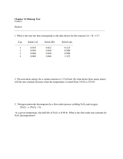
Figure 1. Classification of equilibrium points of a linear
autonomous system. These profiles also arise for non-linear
autonomous systems in linearized approximations.
(3) unstable if there exists an eigenvalue λ of A with real(λ) > 0 for
t → ∞.
The stability of a critical point can also be categorized according to the
values of p = trace(A), q = det(A), and ∆ = p2 − 4q. The following table
summarizes the classification.
Type of Stability
Asymptotically stable
Stable
Unstable
p = λ1 + λ2 q = λ1 λ2
p<0
p≤0
p>0
q>0
q>0
or q < 0
Table 2. Criteria for stability.
12
MIDTERM REVIEW AND SAMPLE EXAM
1.4. Solving ODEs: analytic methods (and numerical methods to
be covered later). Here, we describe various techniques for solving ODEs.
We begin by reviewing methods for solving a single ODE, or scalar differential equation. We then proceed to solving systems of ODEs. A list of the
techniques we covered in this course is as follows:
• Linear first-order ODE: separation of variables.
• Non-linear first-order ODE: exact equations and integrating factors,
linearization, and reduction to linear form.
• Linear first-order constant coefficient (systems) of ODE(s): the general solution of the nonhomogenous problems, the homogenous solution and the eigenproblem, and the particular solution and the
methods of undetermined coefficients and variation of parameters.
• Numerical methods for solving ODEs: Euler’s method as a simple
example.
1.4.1. Non-linear first-order ODE. Some nonlinear ODEs can be reduced to
a linear ODE, for example, the first-order Bernoulli equation
y 0 + p(t)y = g(t)y α ,
α ∈ R.
If we take u(t) = [y(t)]1−α , then u0 (t) = (1 − α)y(t)−α y 0 . Substituting into
the ODE gives
u0 (t) = (1 − α)y(t)−α y 0 = (1 − α)y(t)−α (gy α − py) = (1 − α)(g − pu)
or
u0 + (1 − α)pu = (1 − α)g,
which is a first-order linear system for u. An important example of the
Bernoulli equation results when we set α = 2, p(t) = −A, and g(t) = −B in
which case we have
y 0 = Ay − By 2 .
The equation for u is then
u0 (t) + Au = B,
which has solution
u(t) = ce−At + B/A,
implying
y=
1
1
= −At
.
u
ce
+ B/A
MIDTERM REVIEW AND SAMPLE EXAM
13
1.4.2. Linear second-order ODE: the general solution. Here, we consider the
linear second order IVP
y 00 + p(t)y 0 + q(t)y = g,
y(t0 ) = c1 , y( t0 )0 = c2 .
We assume that p, q, g are continuous functions on some interval I containing
t0 such that there exists a unique solution y.
Remark 1.27. The solution set of the homogenous problem forms a vector
space, that is, (1) y = 0 is a solution and, (2) if α, β ∈ R and x and y are
solutions to the homogenous problem, then αx + βy is a solution:
(αx + βy)00 + p(αx + βy)0 + q(αx + βy) = α(x00 + px0 + qx) + β(y 00 + py 0 + qy)
= α · 0 + β · 0 = 0.
Remark 1.28 (General solution). All solutions of the homogenous problem
can be written as
y = c1 y (1) + c2 y (2) ,
where c1 , c2 ∈ R are arbitrary constants that are uniquely determined by the
initial conditions, provided that the solutions y (1) and y (2) form a basis or
fundamental system. This, in turn, holds true if and only if y (1) and y (2)
are linearly independent, or the Wronskian
W (t) = (y (2) (t))0 y (1) (t) − y (2) (t)(y (1) (t))0 6= 0.
We note that it is sufficient to check that this condition holds for any value
of t.
Example 1.29 (Constant coefficients). Consider the case of a homogenous
second-order linear constant coefficient ODE:
y 00 + ay 0 + by = 0.
Then, we derive the solution by setting y = eλt into the ODE, which gives
(after canceling the common exponential term) the characteristic (quadratic)
polynomial:
λ2 + aλ + b = 0,
whose two roots, λ1 , λ2 give us a solution of the form:
y = c1 eλ1 t + c2 eλ2 t .
There are three possible cases for the roots
√
√
a
a2 − 4b2
a
a2 − 4b
λ1 = − +
λ2 = − −
.
2
,
2
2
(1) Two distinct real roots: λ1 6= λ2 ∈ R. In this case, the solution is
y = c1 eλ1 t + c2 eλ2 t .
(2) Double real roots: λ1 = λ2 = − a2 ∈ R. In this case, the solution is
a
a
y = c1 e− 2 t + c2 te− 2 t .
14
MIDTERM REVIEW AND SAMPLE EXAM
(3) Two complex conjugate roots: λ1 = − a2 + iµ, λ2 = − a2 − iµ. In this
√
case, µ = 4b − a2 > 0 and the solution is
a
y = e− 2 t (c1 cos(µt) + c2 sin(µt)).
Here, Euler’s formula was used: ea+ib = ea eib = ea (cos b + i sin b).
Example 1.30 (Euler-Cauchy equation). Another important second-order
linear ODE is the Euler-Cauchy equation:
t2 y 00 + aty 0 + by = 0.
This system can be reduces to a constant coefficient problem in x by substituting y = tr , since then t0 = rt(r−1) and t00 = r(r − 1)t(r−2) , implying
that
r(r − 1) + ar + b = r2 + (a − 1)r + b = 0.
The roots r1 and r2 of this quadratic polynomial give the solutions to the
system:
y = c1 tr1 + c2 tr2 .
Given the solution to the homogenous problem, one can find the general solution to the corresponding nonhomogenous ODE using various techniques, for example the methods of undetermined coefficients and variation
of parameters. We review these techniques for ODE systems in the next
section, noting that they can also be applied in the case of a scalar equation
in a similar way.
1.4.3. Systems of linear constant coefficient ODEs. Here, we consider solving constant coefficient linear ODE systems
y 0 = Ay + g(t),
A ∈ Rn×n ,
y ∈ Rn .
As discussed in Section 1.2, we solve for the general solution of the nonhomogenous system
y = y (h) + y (p) ,
by first computing the solution for y (h) , the solution of the homogenous
problem, and then using the methods of undetermined coefficients or variation of parameters to find y (p) , the particular solution. Examples of how to
use the latter methods to find y (p) are found in the sample exam.
The general solution of the homogenous system is given by (see, Definition
1.12)
y = c1 x(1) eλ1 t + c2 x(2) eλ2 t + ... + cn x(n) eλn t ,
where λ1 , λ2 , ..., λn are the eigenvalues of A, i.e, the roots of the characteristic polynomial det(A − λI) (a polynomial of degree n in λ), and x(1) , ..., x(n)
the corresponding eigenvectors. We note that if the λi , i = 1, .., n, are
distinct, then one can show that the eigenvectors are linearly independent.
MIDTERM REVIEW AND SAMPLE EXAM
15
2. Linear Algebra
We first state basic definitions and axioms for vectors and matrices. Then,
we review some related concepts from Linear Algebra and apply these ideas
to the solution of linear systems.
2.1. Vectors and Matrices. We consider rectangular matrices


a11 . . . a1n

..  ∈ Rm×n .
..
A =  ...
.
. 
am1 . . . amn
Note that when n = 1 we obtain a column vector
 
x1
 .. 
x =  .  ∈ Rm
xm
and when m = 1 we obtain a row vector
y = y1 . . . ym ∈ Rm .
The basic operations of addition and multiplication among constants α ∈
R, vectors x ∈ Rn , and matrices A ∈ Rm×n are as follows:
• Addition of two matrices C = A + B ∈ Rm×n is defined elementwise
such that cij = ai,j + bi,j and results in the matrix

 
 

a11 . . . a1n
b11 . . . b1n
a11 + b11 . . . a1n + b1n


.. + ..
..  = 
..
..
..
..
..
A+B =  ...
.
.
.
.
.   .
.  
.
.
am1 . . . amn
bm1 . . . bmn
am1 + bm1 . . . amn + bmn
• Multiplication of a matrix, A, by a constant, α, is defined elementwise and results in the matrix:
αA = [αaij ],
i = 1, ..., m,
j = 1, , , ., , , n.
• Multiplication of a vector, x, by a matrix, A, results in the vector:
 Pn

a1j xj
Pj=1
 n a2j xj 
 j=1

Ax = 
 ∈ Rm .
..


.
Pn
j=1 amj xj
• Multiplication of a matrix
in the matrix
 Pn
l=1 a1l bl1

..
AB = 
Pn .
l=1 aml bl1
A ∈ Rm×n by a matrix B ∈ Rn×k results

Pn
...
l=1 a1l blk

..
m×k
..
.
∈R
.
Pn .
...
l=1 aml blk
Note that in general AB 6= BA.
16
MIDTERM REVIEW AND SAMPLE EXAM
Given the matrix

a11
 a21

A =  ..
 .
a12
a22
..
.

a1n
a2n 

..  ,
. 
...
...
..
.
am1 am2 . . . amn
its traspose is defined as

a11
 a12

AT =  ..
 .
a21
a22
..
.
a1n a2n

. . . am1
. . . am2 

..  .
..
.
. 
. . . amn
Note that
(AB)T = B T AT .
There are several classes of matrices that arise often in parctice:
(1) A square matrix, D, is diagonal if dij = 0 for i 6= j:



D=

d11
0
0
..
.
d22
..
.
...
0
...
..
.
..
.
0

0
.. 
. 
.
0 
dnn
(2) The identity matrix is a diagonal matrix where all the diagonal elements are equal to one:

... 0
. . .. 

. .
0 1
I = . .
.
.
 .. . . . . 0
0 ... 0 1

1
0
(3) A square matrix is symmetric if AT = A or aij = aji , i, j = 1, ..., n.
(4) A square matrix is skew symmetric if AT = −A or aij = −aji , i, j =
1, ..., n. Note that skew symmetric matrices have a zero diagonal
aii = −aii = 0, i = 1, ..., n.
(5) An upper triangular matrix, U , is defined as uij = 0, i > j:


u11 u12 . . . u1n
 0 u22 . . . u2n 


U =  ..
..  .
..
..
 .
.
.
. 
0
...
0
unn
MIDTERM REVIEW AND SAMPLE EXAM
(6) A lower triangular matrix,

l11

l
L =  21
 ...
ln1
17
L, is defined as lij = 0, j > i:

0 ... 0
. 
.
l22 . . .. 
.
.. . .
. 0
.
ln2 . . . lnn
Definition 2.1. The inverse of a square matrix, A, is denoted by A−1 and
satisfies:
A−1 A = AA−1 = I.
Example 2.2. Consider the case where n = 2 such that:
a11 a12
A=
.
a21 a22
The inverse of A is
A
−1
1
=
det (A)
a22 −a12
,
−a21 a11
where det(A) = a11 a22 − a21 a12 is the determinant of the matrix. This
implies that A−1 exists if and only if det(A) 6= 0. To check that this is
indeed the inverse of the matrix of A we compute
1
a22 −a12
a11 a12
−1
A A =
a21 a22
det (A) −a21 a11
1
a11 a12
a22 −a12
=
−a21 a11
det (A) a21 a22
1 0
=
.
0 1
Theorem 2.3. The result in the example for n = 2 also holds for general
matrices A ∈ Rn×n , that is, A−1 exists if and only if det (A) 6= 0.
2.2. Vector Spaces.
Definition 2.4. A vector space, V, is a mathematical structure formed by
a collection of elements called vectors, which may be added together and
multiplied (”scaled”) by numbers, called scalars. Note that the elements of a
vector space need not be vectors v ∈ Rm , they can also be functions, matrices,
etc.
The operations of vector addition and scalar multiplication must satisfy certain requirements, called axioms, listed below. Let u, v, w ∈ V be arbitrary
vectors and let α, β ∈ K be arbitrary scalars.
(1) Associativity of addition u + (v + w) = (u + v) + w.
(2) Commutativity of addition: u + v = v + u.
(3) Identity element of addition: there exists an element 0 ∈ V, called
the zero vector, such that v + 0 = v for all v ∈ V.
18
MIDTERM REVIEW AND SAMPLE EXAM
(4) Inverse elements of addition: for every v ∈ V, there exists an element
−v ∈ V, called the additive inverse of v, such that v + (−v) = 0.
(5) Distributivity of scalar multiplication with respect to vector addition:
α(u + v) = αu + αv.
(6) Distributivity of scalar multiplication with respect to field addition:
(α + β)v = αv + βv.
(7) Compatibility of scalar multiplication: α(βv) = (αβ)v.
(8) Identity element of scalar multiplication: 1v = v, where 1 denotes
the multiplicative identity in the field K.
The requirement that vector addition and scalar multiplication be (external) binary operations includes (by definition of binary operations) a
property called closure: that u + v and αv are in V for all α ∈ K, and
u, v ∈ V. This follows since a binary operation on a set is a calculation
involving two elements of the set (called operands) and producing another
element of the set, in this case V. For the field K, the notion of an external
binary operation is needed, which is defined as a binary function from K ×S
to S.
P
Examples of vector spaces are V = Rm and V = {p(x)|p(x) = i αi xi }.
The latter polynomial space is infinite dimensional, whereas the former Euclidian space is finite dimensional.
Definition 2.5. A nonempty subset W of a vector space V that is closed
under addition and scalar multiplication (and therefore contains the 0-vector
of V) is called a subspace of V.
Remark 2.6. To prove that W is a subspace, it is sufficient to prove (1)
0 ∈ W and (2) for any u, v ∈ W and any α, βK, αu + βv ∈ W.
Definition 2.7. If S = {v1 , ...vn } is a finite subset of elements of a vector
space V, then the span is
n
X
span(S) = u|u =
αi vi , αi ∈ K .
i=1
The span of S may also be defined as the set of all linear combinations of
the elements of S, which follows from the above definition.
Definition 2.8. A basis B of a vector space V over a field K is a linearly
independent subset of V that spans V. In more detail, suppose that B =
{v1 , ..., vn } is a finite subset of a vector space V over a field K. Then, B is
a basis if it satisfies the following conditions:
(1) The linear independence property: if
α1 v1 + ... + αn vn = 0,
then α1 = ... = αn = 0; and
(2) The spanning property: for every v ∈ V it is possible to choose
α1 , ..., αn ∈ K such that
v = α1 v1 + ... + αn vn .
MIDTERM REVIEW AND SAMPLE EXAM
19
Definition 2.9. The dimension of a vector space V is dim V = |B|, where
B is a basis for V.
Remark 2.10. We proved the following useful results in class:
(1) The coefficients αi are called the coordinates of the vector v with
respect to the basis B, and by the first property they are uniquely
determined.
(2) Given a vector space V with dim V = n, any linearly independent set
of n vectors forms a basis of V and any collection of n + 1 vectors
is linearly dependent. Thus, the dimension is the maximum number
of linearly independent vectors in V.
The above results all follow from the following basic result.
Lemma 2.11. Let V be a vector space. Assume that the set of vectors
V = {v1 , ..., vn } spans V and that the set of vectors W = {w1 , ..., wm } is
linear independent. Then, m ≤ n and a set of the form
{w1 , ..., wm , vi1 , ..., vin−m }
spans V .
Proof. Assume vi 6= 0 for some i so that V =
6 {0}, else wi ∈ V can not
be linearly
independent
for
any
m
≥
1.
Since
V spans V it follows that
P
w1 = i αi vi and since w1 6= 0, we have that αj 6= 0 for some j. Thus
X
1
vj =
w1 −
αi vi ,
αj
i6=j
implying that the set
{w1 , v1 , ..., vj−1 , vj+1 , ..., vn }
spans V. Repeating this argument, since this updated set spans V
X
w2 = βw1 +
αi vi 6= 0,
i6=j
and thus
{w1 , w2 , v1 , ..., vj−1 , vj+1 , ..., vn }
must be linearly dependent. Now, since w1 and w2 are linearly independent,
it must be that αk 6= 0 for some k 6= j (else w2 = βw1 ). Thus, the set
{w1 , w2 , v1 , ..., vj−1 , vj+1 , ..., vk−1 , vk+1 , ..., vn }
spans V. Repeating the same argument another m-2 times gives that
{w1 , ..., wm , vi1 , ..., vin−m }
spans V.
Next, assume m > n. Then after n steps
{w1 , ..., wn }
20
MIDTERM REVIEW AND SAMPLE EXAM
spans V and after n + 1 steps
{w1 , ..., wn , wn+1 }
is linearly dependent, a contradiction. Thus, m ≤ n.
2.3. Linear systems of equations. Here, we consider the matrix equation
Ax = b, A ∈ Rm×n , b ∈ Rm , and x ∈ Rn , which represents a system of m
linear equations with n unknowns:
a1,1 x1 + a1,2 x2 + ... + a1,n xn = b1 ,
a2,1 x1 + a2,2 x2 + ... + a2,n xn = b2 ,
..
.
am,1 x1 + am,2 x2 + ... + am,n xn = bn ,
where, x1 , ..., xn are the unknowns, ai,j , 1 ≤ i, j ≤ n are given coefficients
and b1 , ..., bn are constants, imposing constraints that these equations must
satisfy. Note that the unknowns appear in each of the equations and as such
we must find their values such that all equations are satisfied simultaneously.
There are n columns of A (vectors) denoted as


a1j
 a2j 


(j)
a =  ..  , j = 1, ..., n,
 . 
amj
and m row vectors
a(i) = ai1 ai2 . . . ain ,
i = 1, ..., m.
Definition 2.12. The column space, a vector space, is defined as colsp(A) =
span(a(1) , ..., a(n) and the row space, also a vector space, is defined as rowsp(A) =
span(a(1) , ..., a(m) .
Definition 2.13. The maximum number of linearly independent rows in a
matrix A is called the row rank of A, which is equal to the maximum number
of linearly independent columns in A, referred to ass the column rank. Since
the two are equal, we will not distinguish between them and write rank(A)
to denote both.
Remark 2.14. Note that from our discussion of vector spaces we have that
rank(A) = dim colsp(A) = dim rowsp(A).
Finally, we proved the following existence and uniqueness theorem for this
linear system.
Theorem 2.15. Consider the linear system Ax = b, A ∈ Rm×n , b ∈ Rm ,
.
and x ∈ Rn and let A˜ = [A..b]. Then, the system
˜ = rank(A);
(1) is consistent (the solution exists) if rank(A)
˜
(2) has a unique solution if rank(A) = rank(A) = n;
MIDTERM REVIEW AND SAMPLE EXAM
21
˜ = rank(A) < n.
(3) has infinitely many solutions if rank(A)
Proof. The first two parts are proved in the sample exam. Thus, we prove
˜ = rank(A) = r < n. Then
only the last statement here. Assume rank(A)
note that
n
X
b=
xi a(i) ,
i=1
where there are r linearly independent columns in A and then n − r which
are linearly combinations of these r columns. We reorder the columns of the
ˆ which has as its first r columns those columns from
matrix A to obtain A,
A that are linearly independent:
r
n
X
X
b=
x
ˆi a
ˆ(i) +
x
ˆi a
ˆ(i) .
i=1
i=r+1
Note that these first r columns form a basis, B = {ˆ
a(1) , ..., a
ˆ(r) } for colsp(A) =
ˆ Now, since the last n − r columns of Aˆ can be written as linear
colsp(A).
combinations of elements of B, we can write them as follows:
r
X
a(i) =
αij a
ˆ(j) , i = r + 1, ..., n,
j=1
which gives the system
b=
r
X
x
ˆi a
ˆ(i) +
i=1
n
X
x
ˆi
i=r+1
r
X
αij a
ˆ(j) .
j=1
Collecting terms, we arrive at a reduced system:
r
X
b=
yi a
ˆ(i) ,
i=1
where
yi = x
ˆi + βi ,
n
X
βi =
x
ˆl αli .
l=r+1
Now, by the second result of the theorem, i.e., (2), the yi , i = 1, ..., r are
uniquely determined. Thus, once we fix the values of xi , i = r + 1, ..., n,
then we can solve for the values of xi , i = 1, ..., r.
Example 2.16. Consider the matrix


1 2 0
A = 1 2 1
0 0 0
and the right hand side
 
b1

b = b2  .
b3
22
MIDTERM REVIEW AND SAMPLE EXAM
Note that rank(A) = 2 and in order for
˜ = 2. Now,
that b3 = 0, such that rank(A)
many solutions to Ax = b. Our approach

1 0
Aˆ = 1 1
0 0
a solution to exist we must have
we show that there exist infinitely
follows the proof above. Let

2
2 .
0
Then,
b =
=
=
=
 
 
 
1
0
2
x
ˆ1 1 + x
ˆ2 1 + x
ˆ3 2
0
0
0
 
 
 
1
0
1
x
ˆ1 1 + x
ˆ2 1 + 2ˆ
x3 1
0
0
0
 
 
1
0
(ˆ
x1 + 2ˆ
x3 ) 1 + x
ˆ2 1
0
0
 
 
1
0
y1 1 + y2 1 ,
0
0
with y1 = x
ˆ1 + 2ˆ
x3 and y2 = x
ˆ2 . Now, the solution to the system in y is
y1 = b1 and y2 = b2 − b1 . Thus, b1 = x
ˆ1 + 2ˆ
x3 and x
ˆ2 = b2 − b1 . Thus,
x
ˆ1 = b1 − 2ˆ
x3
x
ˆ2 = b2 − b1
x
ˆ3 ∈ R.
Note that x
ˆ3 is a free variable and can be chosen arbitrarily.
MIDTERM REVIEW AND SAMPLE EXAM
23
3. Midterm Sample Exam
(1) (4.1 #14.)
Undamped motions of an elastic spring are governed by the equation
my 00 + ky = 0 or my 00 = −ky,
where m is the mass, k the spring constant, and y(t) the displacement
of the mass from its equilibrium position. Modeling the masses on
the two springs we obtain the following system of ODEs:
m1 y100 = −k1 y1 + k2 (y2 − y1 )
m2 y200 = −k2 (y2 − y1 )
for unknown displacements y1 (t) of the first mass m1 and y2 (t) of
the second mass m2 . The forces acting on the first mass give the first
equation and the forces acting on the second mass give the second
ODE. Let m1 = m2 = 1, k1 = 3, and k2 = 2 which gives the system
00 −5 2
y1
y1
00
=
.
y =
00
y2
2 −2
y2
Solve the equation by substituting the function y = xeωt into the
ODE.
Solution.
y 00 = ω 2 xeωt = Axeωt .
Setting ω 2 = λ and dividing by eωt gives the eigenproblem
Ax = λx,
which we solve for x and λ to find the solution.
Now,
det(A − λI) = (−5 − λ)(−2 − λ) − 4 = λ2 + 7λ + 6 = (λ + 1)(λ + 6) = 0.
Thus, the eigenvalues are λ1 = −1 and λ2 = −6. The eigenvector
for λ1 = −1 is obtained by solving
−4 2
x1
0
=
.
2 −1
x2
0
1
Which gives the eigenvector x(1) =
. Similarly, the eigenvector
2
2
for λ2 = −6 is x(2) =
.
−1
√ √
√
√
Notice that ω = ± λ, −1 = i and −6 = i 6. Thus,
√ √
y = x(1) c1 eit c2 e−it + x(2) c3 ei 6t + c4 e−i 6t .
Now, using Euler’s formula eit = cos(t) + i sin(t) it follows that
√
√
y = a1 x(1) cos(t) + b1 x(1) sin(t) + a2 x(2) cos( 6t) + b2 x(2) sin( 6t),
24
MIDTERM REVIEW AND SAMPLE EXAM
where a1 = c1 + c2 , b1 = i(c1 − c2 ), a2 = c3 + c4 , b2 = i(c3 − c4 ).
These four arbitrary constants are specified by the initial conditions.
Remarks: in components, the solution reads:
√
√
y1 = a1 cos(t) + b1 sin(t) + 2a2 cos( 6t) + 2b2 x(2) sin( 6t),
√
√
y2 = 2a1 cos(t) + 2b1 sin(t) − a2 cos( 6t) − b2 x(2) sin( 6t)
The first two terms in y1 and y2 give a slow harmonic motion, and
the last two a fast motion. The slow motion occurs if both masses
are moving in the same direction, for example, if a1 = 1 and the
other three constants are zero. The fast motion occurs if at each
instant the two masses are moving in opposite directions, so that
one spring is extended and the other compressed. For example if
a2 = 1 and the other constants are zero. Depending on the initial
conditions, one or the other of these motions, or superposition of
both of them will result.
(2) (Review # 28) Find the location of the critical points of the system:
y10 = cos(y2 )
y20 = 3y1
Can the type of the critical points be determined from the linearized
system? Be sure to justify this claim. If your answer is yes, then
find the type of the critical points.
Solution. The critical points are given by (y1 , y2 ) such that
f1 (y2 ) = cos(y2 ) = f2 (y1 ) = 3y1 = 0.
Thus, their are infinitely many critical points given by
π
,
0, 2n + 1
2
where n is any integer. The transformation y → y˜ that maps the
critical points to the origin is given by
π
y˜1 = y1 and y˜2 = y2 − (2n + 1) .
2
Thus, we obtain a system in y˜ by substituting
π
y1 = y˜1 and y2 = y˜2 + (2n + 1)
2
into the system for y. Letting n = 0 we have the critical point (0, π2 ),
for which the system in y˜ reads
π
y˜10 = cos(˜
y2 + ) = − sin(˜
y2 )
2
y˜20 = 3˜
y1
MIDTERM REVIEW AND SAMPLE EXAM
25
To determine the type of this critical point we linearize the system:
y˜0 ≈ Jf (0)˜
y , where Jf (0) is the Jacobian matrix
0 − cos(0)
0 −1
Jf (0) =
=
.
3
0
3 0
Note that f1 (˜
y2 ) = − sin(˜
y2 ) ∈ C 1 , f2 (˜
y1 ) = 3˜
y1 ∈ C 1 and
det Jf (0) 6= 0 such that the type and stability of the critical points
of the nonlinear system coincide with the linearized system.
Now,
√
2
the eigenvalues satisfy λ + 3 = 0, so that λ± = ±i 3. Thus,
p = trace(Jf (0)) = λ+ + λ− = 0 and det(Jf (0)) = λ+ λ− = 3 and,
thus, the critical point is a center. Note that by periodicity of cos(),
all the critical points (0, (4n + 1) π2 ) are centers as well, since in such
case
π
π
π
cos y˜2 + 4n + 1
= cos y˜2 + 2nπ +
= cos y˜2 +
.
2
2
2
Next, consider n = −1 such that the critical point is (0, − π2 ).
Then,
π
y˜10 = cos(˜
y2 − ) = sin(˜
y2 )
2
y˜20 = 3˜
y1
implying
0 cos(0)
0 1
Jf (0) =
=
.
3
0
3 0
√
Here, the eigenvalues satisfy λ2 − 3 = 0 and, thus, λ± = ± 3. This
gives p = 0 and q = −3 which implies the critical point is a saddle
point. Note that due to periodicity, all of the critical points of the
form (0, (4n − 1) π2 ) are saddle points.
(3) Consider the nonhomogenous system of ODEs:
0
y (t) = Ay(t) + g(t),
−3 1
A=
,
1 −3
−6 −2t
g(t) =
e .
2
Show that a unique solution exists for initial conditions y(0) = s.
Then compute the solution.
Solution. To show that a unique solution exists we consider the
right hand side of the equaiton:
−3y1 + y2 − 6e−2t
f (t, y1 , y2 ) =
.
y1 − 3y2 + 2e−2t
Since the equation is a constant coefficient linear system, it is sufficient to note that the exponential terms corresponding to the rhs,
e−2t , are continuously differentiable at t = 0 (actually for any t).
26
MIDTERM REVIEW AND SAMPLE EXAM
Next, we compute the solution to the homogenous system g(t) =
0. The eigenvalues satisfy (λ + 2)(λ + 4) = 0, and so λ1 = −2 and
λ2 = −4. The corresponding eigenvectors are
1
1
(1)
(2)
x =
and x =
,
1
−1
giving the homogenous solution
1
1 −2t
(h)
e−4t .
e
+ c2
y = c1
−1
1
Now, to find a particular solution, we can use (1) the method of
undetermined coefficients or (2) variation of parameters.
For the undetermined coefficients approach, we consider the particular solution
y (p) = ute−2t + ve−2t ,
since the e−2t in g(t) is a solution to the homogenous problem. Our
task is then to determine the coefficients u and v. This can be done
by plugging y (p) into the system of ODEs:
−6 −2t
(p) 0
−2t
−2t
−2t
−2t
−2t
(y ) = ue
− 2ute
− 2ve
= Aute
+ Ave
+
e .
2
Now, equating coefficients
• of the te−2t terms gives Au = −2u. Thus, u is a solution to the
homogenous system
−3 + 2
1
u1
0
=
.
1
−3 + 2
u2
0
Thus, u1 = u2 = c, for any c ∈ R.
• of the e−2t terms gives
c
u − 2v = Av + w, u =
,
c
−6
w=
2
or
c
v1
−3 1
v1
−6
−2
=
+
.
c
v2
1 −3
v2
2
This gives the system
−1 1
v1
6+c
=
,
1 −1
v2
−2 + c
which is consistent if c = −2, since then, the right hand side is
an element of the column space of the given matrix:
4
−1
∈ span
.
−4
1
MIDTERM REVIEW AND SAMPLE EXAM
27
Note that since rank(A) < n = 2, there exist infinitely many
solutions to this linear system:
1
−1
−1
4
= (v1 − v2 )
,
+ v2
= v1
−1
1
1
−4
implying v2 −v1 = 4 or v2 = v1 +4, where v1 is the free variable.
Finally, plugging u and v into the definition of y (p) and adding this
to y (h) gives the general solution to the nonhomogenous problem:
1
−2
v1
1 −2t
−4t
−2t
(h)
(p)
e
+
te
+
e−2t .
e
+ c2
y = y + y = c1
−1
−2
v1 + 4
1
Note that the solution is valid for any v1 ∈ R. Once v1 has been
selected, the constants c1 and c2 are uniquely determined by the
initial conditions, y1 (t0 ) = s1 and y2 (t0 ) = s2 .
Next, given a solution to the homogenous system, we find a particular solution using the method of variation of parameters. This
approach is easy to understand if we write the solution of the homogenous system, y (h) , solving
y 0 = Ay + g,
g ≡ 0,
in terms of the fundamental matrix. Let,
1 −2t
1
(1)
(2)
y =
e , y =
e−4t .
1
−1
Then,
y (h) (t) = Y (t)c,
where
Y = y (1) y (2) =
e−2t e−4t
e−2t −e−4t
and c =
c1
.
c2
The idea is then to write the particular solution in the form y (p) =
Y (t)u(t) and plug this into the nonhomogenous system to find u(t).
Substituting into the equation gives
Y 0 u + Y u0 = AY u + g.
Noting that Y 0 = AY , it follows that Y 0 u = AY u, which gives
Y 0 u = g ⇒ u0 = Y −1 g,
where
Y
−1
−1
=
−2e−6t
−4t
1 e2t e2t
−e
−e−4t
=
.
−e−2t e−2t
2 e4t −e4t
Thus,
u0 =
1
2
e2t e2t
e4t −e4t
−2
−6e−2t
=
.
−4e2t
2e−2t
28
MIDTERM REVIEW AND SAMPLE EXAM
Integrating we get
u(t) =
−2t
−2e2t
and
y
(p)
−2t
−2t
−2
v1
e
e−4t
−2t − 2 −2t
−2t
= Y (t)u(t) = −2t
=
e
=
te +
e−2t
−2t + 2
−2
v1 + 4
−2e2t
e
−e−4t
for v1 = −2.
Linear Algebra
(4) Show that the set of all 3 × 3 skew symmetric matrices, i.e.,
V = {A ∈ R3×3
such that
AT = −A},
is a vector space and find the dimension and a basis for V .
Solution. Note that if A ∈ R3×3 such that AT = −A, then we
can write A as


0
a1 a2
0
a3  ,
A = −a1
−a2 −a3 0
so that at most three entries of the nine total entries in the matrix
A can be chosen independently. Now, taking


0
b1 b2
0 b3  ,
B = −b1
−b2 −b3 0
we have


0
αa1 + βb1
αa2 + βb2
0
αa3 + βb3  ,
αA + βB = −(αa1 + βb1 )
−(αa2 + βb2 ) −(αa3 + βb3 )
0
which is again a skew symmetric matrix. Moreover the 3 × 3 zero
matrix is skew symmetric, since then aij = −aji , as required. Thus,
V is a vector space. A basis of V is

0 1 0
−1 0 0 ,
0 0 0



0 0 1
 0 0 0 ,
−1 0 0

and

0 0 0
0 0 1  ,
0 −1 0
so that dim V = 3.
(5) Consider the linear system of equations
x ∈ Rn , and b ∈ Rm .
Define the augmented matrix A˜ = A b ∈ Rm×(n+1) . (a) Show that
˜ = rank(A). (b) Show that
the linear system is consistent iff rank(A)
the system has a unique solution iff this common rank is equal to n.
Ax = b,
A ∈ Rm×n ,
MIDTERM REVIEW AND SAMPLE EXAM
29
P
Solution. To prove (a), note that b = ni=1 xi a(i) and, also that
˜ =
dim colsp(A) = rank(A), implying b ∈ colsp(A) iff rank(A)
rank(A).
Next, to prove (b) we assume that there exist two solutions, say
x, y ∈ Rn such that Ax = Ay = b. Then,
n
X
Ax − Ay = A(x − y) =
(xi − yi )a(i) = 0.
i=1
Now, since rank(A) = n, it follows that the columns of A are linearly
independent, implying
xi − yi = 0,
for i = 1, ..., n,
or x = y.
In the other direction, we assume that Ax = b has a unique solution and then pick a particular right hand side b = 0. Then, x = 0
is a solution and by assumption it is unique. This, then implies that
n
X
Ax =
xi a(i) = 0
i=1
has only the trivial solution x = 0. Thus, the columns of a(i) ,
i = 1, ..., n, are linearly independent and rank(A) = n. By our as˜ =
sumption that a solution exists and part (a) it follows that rank(A)
rank(A).