1. science
2. physics

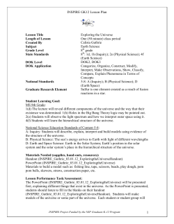
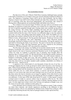
The Astronomical Journal, 144:110 (7pp), 2012 October
C 2012.
doi:10.1088/0004-6256/144/4/110
The American Astronomical Society. All rights reserved. Printed in the U.S.A.
FITTING THE UNION2.1 SUPERNOVA SAMPLE WITH THE Rh = ct UNIVERSE
F. Melia1
Department of Physics, The Applied Math Program, and Steward Observatory, The University of Arizona, Tucson, AZ 85721, USA; [email protected]
Received 2012 June 18; accepted 2012 August 2; published 2012 September 11
ABSTRACT
The analysis of Type Ia supernova data over the past decade has been a notable success story in cosmology. These
standard candles offer us an unparalleled opportunity to study the cosmological expansion out to a redshift of ∼1.5.
The consensus today appears to be that ΛCDM offers the best explanation for the luminosity–distance relationship
seen in these events. However, a significant incompatibility is now emerging between the standard model and
other equally important observations, such as those of the cosmic microwave background. ΛCDM does not provide
an accurate representation of the cosmological expansion at high redshifts (z 2). It is therefore essential to
re-analyze the Type Ia supernova data in light of the cosmology (the Rh = ct universe) that best represents the
universe’s dynamical evolution at early times. In this paper, we directly compare the distance relationship in ΛCDM
with that predicted by Rh = ct, and each with the Union2.1 sample, and show that the two theories produce
virtually indistinguishable profiles, though the fit with Rh = ct has not yet been optimized. This is because the data
cannot be determined independently of the assumed cosmology—the supernova luminosities must be evaluated by
optimizing four parameters simultaneously with those in the adopted model. This renders the data compliant to
the underlying theory, so the model-dependent data reduction should not be ignored in any comparative analysis
between competing cosmologies. In this paper, we use Rh = ct to fit the data reduced with ΛCDM, and though
quite promising, the match is not perfect. An even better fit would result with an optimization of the data using
Rh = ct from the beginning.
Key words: cosmic background radiation – cosmological parameters – cosmology: observations – cosmology:
theory – distance scale – supernovae: general
a comparative analysis. The consensus today appears to be that
ΛCDM offers the best explanation for the redshift–luminosity
distribution seen in these events, and observational work is now
focused primarily on refining the fits to improve the precision
with which the model parameters are determined.
When these efforts are viewed through the prism of a more
comprehensive cosmological study, however, the situation is
not quite so simple. The reason is that although ΛCDM does
very well in accounting for the properties of Type Ia SNe,
it does poorly in attempts to explain several other equally
important observations, particularly the angular distribution of
anisotropies in the cosmic microwave background (CMB) and
the clustering of matter. For example, the angular correlation
function of the CMB is so different from what ΛCDM predicts
that the probability of it providing the correct expansion history
of the universe near recombination is less than ∼0.03% (Copi
et al. 2009; Melia 2012b). Insofar as the matter distribution is
concerned, ΛCDM predicts a distribution profile that changes
with scale, seemingly at odds with the observed near universal
power law seen everywhere below the BAO (Baryonic Acoustic
Oscillations) scale (∼100 Mpc), leading Watson et al. (2011) to
categorize it as a “cosmic coincidence.”
This disparity is the principal topic we wish to address in this
paper, with a particular emphasis on what the Rh = ct universe
has to say about the universal expansion implied by the Type Ia
SN data. As we have shown in earlier papers (see, e.g., Melia
2007, 2012a, 2012b; Melia & Shevchuk 2012), and summarized
in Section 2, the Rh = ct universe is more effective than
ΛCDM in accounting for the properties of the CMB. This raises
the question of whether ΛCDM is really revealing something
different about the local universe—as opposed to what happened
much earlier, closer to the time of last scattering—or whether
it is possible for us to understand how and why it may simply
1. INTRODUCTION
We now have several methods at our disposal for probing
the expansion history of the universe, but none better than the
use of Type Ia supernovae (SNe; Perlmutter et al. 1998, 1999;
Garnavich et al. 1998; Schmidt et al. 1998; Riess et al. 1998).
Producing a relatively well-known luminosity, these events
function as reasonable standard candles, under the assumption
that the power of both near and distant events can be standardized
with the same luminosity versus color and lightcurve shape
relationships.
Over the past decade, the combined efforts of several groups
have led to an impressive accumulation of events and an ever
improving quality of individual measurements. More recently,
Kowalski et al. (2008) devised a framework for analyzing
such data sets in a homogeneous manner, creating an evolving
compilation currently known as the Union2.1 sample (see
Suzuki et al. 2012 for its most recent incarnation), which
contains 580 SN detections. At the highest redshifts (z > 1), the
Hubble Space Telescope plays a key role, not only in discovering
new events, but also in providing high-precision optical and
near-IR lightcurves (see, e.g., Riess et al. 2004; Kuznetsova
et al. 2008; Dawson et al. 2009). While at lower redshifts,
extensive surveys from the ground continue to grow the sample
at a sustainably high rate (see references cited in Suzuki et al.
2012).
These events constrain cosmological parameters through a
comparison of their apparent luminosities with those predicted
by models over a range of redshifts. The key point of this exercise is that models with different expansion histories predict
specific (and presumably distinguishable) distance versus redshift relationships, which one may match to the observations for
1
John Woodruff Simpson Fellow.
1
The Astronomical Journal, 144:110 (7pp), 2012 October
Melia
be mimicking the expansion history suggested by the Rh = ct
universe at low redshifts.
This is not an easy question to address, principally because of
the enormous amount of work that goes into first establishing the
SN magnitudes, and then carefully fitting the data using the comprehensive set of parameters available to ΛCDM. As we shall
see in Section 3, part of the problem is that the distance moduli themselves cannot be determined completely independently
of the assumed model. This leads to the unpalatable situation
in which the data tend to be somewhat compliant, producing
slightly better fits for the input model than might otherwise occur if they were completely model independent. But even with
these complications, we will show that ΛCDM appears to fit the
SN data well because its seven free parameters allow it to relax
to the Rh = ct universe at low redshifts. In other words, we
suggest that fits to the Union2.1 sample cannot, by themselves,
distinguish between ΛCDM and the Rh = ct universe. The preponderance of evidence therefore rests with the CMB, which
appears to favor the Rh = ct cosmology.
from observations. The problem with this, however, is that the
observations are quite varied and cover disparate properties of
the universe, some early in its history (as seen in the fossilized
CMB) and others more recently (such as the formation of
large-scale structure and the aforementioned distribution of
Type Ia SNe).
In recent work, we have demonstrated why this approach may
be useful in establishing a basis for theoretical cosmology, but
why in the end ΛCDM essentially remains an approximation to
the more precise theory embodied in the Rh = ct universe. What
is lacking in ΛCDM is the overall equation of state, p = −ρ/3,
linking the total pressure p and the total energy density ρ. This
simple relationship is required when the cosmological principle
and the Weyl postulate are adopted together. In consequence,
ΛCDM may “fit” the data in certain restricted redshift ranges,
but it fails in other limits. For example, Rh in ΛCDM fluctuates
about the mean it would otherwise always have (since it must
always be equal to ct), leading to the awkward situation in
which the value of Rh (t0 ) is equal to ct0 today, but in order to
achieve this “coincidence,” the universe had to decelerate early
on, followed by a more recent acceleration that exactly balanced
out the effects of its slowing down at the beginning. In Sections 4
and 5, we shall see how this balancing act functions in a more
quantitative manner (particularly when fitting the Type Ia SN
data), and we shall actually learn that the cancellation is even
more contrived than it seems at first blush.
The problems with ΛCDM begin right at the outset because
of its implied deceleration just after the big bang. This slowing
down brings it into direct conflict with the near uniformity of the
CMB data (see, e.g., Melia 2012a), requiring the introduction
of an ad hoc inflationary phase to rescue it. As shown in Melia
(2012b), however, the recent assessment of the observed angular
correlation function C(θ ) in the CMB simply does not support
any kind of inflationary scenario. We showed in that paper
that, whereas ΛCDM fails to account for the observed shape
of C(θ )—particularly the absence of any correlation at angles
greater than ∼60◦ —the Rh = ct universe explains where C(θ )
attains its minimum value (at θmin ), the correlation amplitude
C(θmin ) at that angle and, most importantly, why there is no
angular correlation at large angles. The chief ingredient in
ΛCDM responsible for this failure to account for the properties
of C(θ ) is inflation, which would have expanded all fluctuations
to very large scales. Instead, the Rh = ct universe did not
undergo such an accelerated expansion, so its largest fluctuations
are limited to the size of the gravitational horizon Rh (te ) at the
time of last scattering.
To be completely fair to the standard model, however, we
also point out that in spite of its failure to account for the
distribution of large-scale fluctuations in the CMB, it does very
well in explaining the large-l power spectrum associated with
fluctuations on scales below ∼1◦ . Recent observations provide
an even more convincing confirmation of the large-l spectrum
predicted by ΛCDM (see, e.g., Hlozek et al. 2012). More
work needs to be carried out to fully understand this disparity.
It could be that unlike the Sachs–Wolfe effect, the physical
processes (such as acoustic fluctuations) influencing the smallscale behavior are much less dependent on the expansion
scenario. There is a hint that this may be happening from
the analysis of Scott et al. (1995), who demonstrated that the
same large-l power spectrum can result from rather different
cosmological models.
The CMB carries significant weight in determining which of
the candidate models accounts for the universal expansion, and
2. THE Rh = ct UNIVERSE
The Rh = ct universe is an FRW cosmology that adheres
very closely to the restrictions imposed on the theory by the
cosmological principle and Weyl’s postulate (Melia 2007; Melia
& Shevchuk 2012). Most people realize that adopting the
cosmological principle means we assume that the universe is
homogeneous and isotropic. But many do not know that this is
only a statement about the structure of the universe at any given
cosmic time t. In order to complete the rationale for the FRW
form of the metric, one also needs to know how the time slices at
different t relate to each other. In other words, one needs to know
whether or not the cosmological principle is maintained from
one era to the next. This is where Weyl’s postulate becomes
essential, for it introduces the equally important assumption
about how the various worldlines propagate forward in time.
Weyl’s postulate says that no two worldlines in the Hubble flow
ever cross. Small, local crossings are, of course, always possible,
and we understand that these are due to small departures from an
overall Hubble expansion. But on large scales, the assumption
that worldlines never cross places a severe restriction on how
the distance between any two points can change with time. This
is the origin of the relationship between the so-called proper
distance R(t) in FRW cosmologies and the universal expansion
factor a(t), such that R(t) = a(t)r, in terms of the unchanging
comoving distance r.
But what has not been recognized until recently is that
when these two basic tenets are taken seriously, they force the
gravitational horizon Rh (more commonly known as the Hubble
radius) to always equal ct. (The proof of this is straightforward
and may be found, e.g., in Melia & Shevchuk 2012, and in
the more pedagogical treatment of Melia 2012a.) It is not
difficult to see that this equality in turn forces the expansion
rate to be constant, so the expansion factor a(t) appearing in
the Friedmann equations must be t/t0 (utilizing the convention
that a(t0 ) = 1 today), where t0 is the current age of the
universe.
Over the past several decades, ΛCDM has developed into
a comprehensive description of nature, which nonetheless is
not entirely consistent with this approach. Instead, ΛCDM
assumes a set of primary constituents (radiation, matter, and an
unspecified dark energy), and adopts a partitioning among these
components that is not theoretically well motivated. ΛCDM is
therefore an empirical cosmology, deriving many of its traits
2
The Astronomical Journal, 144:110 (7pp), 2012 October
Melia
here we have a situation in which ΛCDM cannot explain the
near uniformity of the CMB across the sky without inflation,
yet with inflation it cannot account for the anisotropy of the
CMB on large scales.
This distinction alone already demonstrates the superiority of
the Rh = ct universe over ΛCDM, insofar as the interpretation
of the CMB observations is concerned. But this is only one of
several crucial tests affirming the conclusion that ΛCDM is only
an approximation to the more precise Rh = ct universe. Here
are several other reasons.
again has to do with the finite fluctuation size, limited by
the gravitational horizon Rh (te ) at the time of last scattering.
3. THE UNION2.1 SUPERNOVA SAMPLE
Let us now briefly review the contents of the Union2.1 sample,
and summarize the key steps taken during its assembly. As the
samples have grown and become better calibrated, evidence
has emerged for a correlation between host galaxy properties
and SN luminosities, after corrections are made for lightcurve
width and SN color (Hicken et al. 2009). For example, Type
Ia SNe in early-type galaxies appear to be brighter (by about
0.14 mag) than their counterparts in galaxies of later type. A
similar relationship appears to exist between Hubble residuals
and host galaxy mass (Kelly et al. 2010; Sullivan et al. 2010;
Lampeitl et al. 2010). Uncorrected, such relationships can
lead to significant systematic error in determining the best-fit
cosmology.
Additional sources of uncertainty arise for astrophysical reasons, including the color correction that must be applied to SN
luminosities. The so-called redder–fainter relation apparently
arises from at least two mechanisms: extinction from interstellar dust, and probably some intrinsic relation between color
and luminosity produced by the explosion itself or by the surrounding medium. It is difficult to justify the argument that this
redder–fainter relationship should behave in the same way at
all redshifts, but there is little else one can do because the two
effects are very difficult to disentangle (see, e.g., Suzuki et al.
2012).
Combining the many available data sets into a single compilation (the Union2.1 sample) has obvious advantages, treating all
SNe on an equal footing and using the same lightcurve fitting,
but this process brings its own set of possible errors, including
the fact that the systematics may be different among the various
data sets. As we shall see shortly, this multitude of uncertainties
makes it impossible to determine the SN luminosities without some prior assumption about the underlying cosmological
model.
The procedure for determining each individual Type Ia SN
luminosity requires a fit to the lightcurve using three parameters
(aside from those arising in the cosmological model itself).
These are (1) an overall normalization, x0 , to the time-dependent
spectral energy distribution of the SN; (2) the deviation, x1 , from
the average lightcurve shape; and (3) the deviation, c, from the
mean Type Ia SN B − V color. These three parameters, along
with the assumed host mass, are then combined to form the
distance modulus
1. The Rh = ct universe explains why it makes sense to
infer a Planck mass scale in the early universe by equating
the Schwarzschild radius to the Compton wavelength. In
ΛCDM there is no justifiable reason why a delimiting
gravitational horizon should be invoked in an otherwise
infinite universe (see Melia 2012a for a more pedagogical
explanation).
2. The Rh = ct universe explains why Rh (t0 ) = ct0 today
(because they are always equal). In ΛCDM, this equality
is just one of many coincidences. As we shall see in
subsequent sections of this paper, this awkwardness will
become apparent in how the free parameters in ΛCDM
must be manipulated in order to fit the Type Ia SN data
(see, e.g., Figure 4).
3. The Rh = ct universe explains how opposite sides of
the CMB could have been in equilibrium at the time
(te ∼ 104 –105 years) of recombination, without the need
to introduce an ad hoc period of inflation. Inflation may
be useful for other reasons, but it does not appear to
be necessary in order to solve a non-existent “horizon
problem” (Melia 2012b).
4. The Rh = ct universe explains why there is no apparent
length scale below the BAO wavelength (∼100 Mpc) in the
observed matter correlation function. In their exhaustive
study, Watson et al. (2011) concluded that the observed
power-law galaxy correlation function below the BAO is
simply not consistent with the predictions of ΛCDM, which
requires different clustering profiles of matter on different
spatial scales. These authors suggested, therefore, that the
galaxy correlation function must be a “cosmic coincidence.”
But this is not the case in the Rh = ct universe because
this cosmology does not possess a Jeans length (Melia &
Shevchuk 2012). Since p = −ρ/3, the active gravitational
mass (ρ + 3p) in the Rh = ct universe is zero, so
fluctuations grow as a result of (negative) pressure only,
without any delimiting spatial scale.
5. The fact that ρ is partitioned into ≈27% matter and ≈73%
dark energy is a mystery in ΛCDM. But in the Rh = ct
universe, it is clear why Ωm must be ≈27%, because when
one forces ρ to have the specific constituents ρr , ρm , and ρΛ ,
only the value Ωm ≈ 0.27 will permit the universe to evolve
in just the right way to satisfy the condition Rh (t0 ) = ct0
today. This condition is always satisfied in the Rh = ct
universe, but not in ΛCDM. Yet the observations today
must be consistent with this constraint imposed by the
cosmological principle and the Weyl postulate, so all the
other evolutionary aspects of the ΛCDM cosmology must
comply with this requirement.
6. The observed near alignment of the CMB quadrupole and
octopole moments is a statistically significant anomaly
for ΛCDM, but merely lies within statistically reasonable
expectations in the Rh = ct universe (Melia 2012b). This
true
μB = mmax
< mthreshold
) − MB ,
B + α · x1 − β · c + δ · P (m∗
∗
(1)
where mmax
B is the integrated B-band flux at maximum light, MB
is the absolute B-band magnitude of a Type Ia SN with x1 = 0,
c = 0, and P (mtrue
< mthreshold
) = 0. Also, mthreshold
= 1010 M
∗
∗
∗
is the threshold host galaxy mass used for the mass-dependent
correction, and P is a probability function assigning a probability
that the true mass, mtrue
∗ , is less than the threshold value, when
an actual mass measurement mobs
∗ is made.
It is quite evident that the task of accurately determining μB
for each individual SN is arduous indeed. The Supernova Cosmology Project calls the parameters α, β, δ, and MB “nuisance”
parameters because they cannot be evaluated independently of
the assumed cosmology. They must be fitted simultaneously
3
The Astronomical Journal, 144:110 (7pp), 2012 October
Melia
with the other cosmological parameters, e.g., emerging from
ΛCDM.
But this is quite a serious problem that cannot be ignored, e.g.,
when comparing the overall fits to the data with ΛCDM and the
Rh = ct universe (or any other cosmology, for that matter)
because, as we have already alluded to above, this procedure
makes the data at least somewhat compliant to the assumed
cosmological model.
46
Distance Modulus
44
4. THEORETICAL FITS
The best-fit cosmology is determined by an iterative
χ 2 -minimization of the function
2
χstat
=
42
40
38
36
[μB (α, β, δ, MB ) − 5 log 10(dL (ξ, z)/10 pc)]2
,
2
2
σlc2 + σext
+ σsample
supernovae
34
ΛCDM
32
(2)
a(t0 )
,
a(te )
(4)
(5)
ρ
= Ωr + Ωm + ΩΛ ,
ρc
(6)
we may write
Ω≡
from which we get
a0
ae
da
,
Ωr + aΩm /a0 + (a/a0 )4 ΩΛ
1.2
1.4
(10)
re = ln
t0
.
te
(11)
1+z=
a(t0 )
,
a(te )
(12)
With
(7)
it is easy to see that
we get
c 1
re =
H0 a02
1
a(t0 )
t0
= ,
a(te )
te
where, in obvious notation, Ωr ≡ ρr /ρc , Ωm ≡ ρm /ρc , and
ΩΛ ≡ ρΛ /ρc .
In a spatially flat universe (k = 0), Ω = 1, so if we assume
that ρr ∼ a −4 , ρm ∼ a −3 , and ρΛ = constant then, from the
geodesic equation,
c dt = −a(t) dr,
0.8
Figure 1 shows the Union2.1 sample of 580 Type Ia SNe,
along with the best-fit ΛCDM model, in which dark energy
is a cosmological constant, Λ, its equation-of-state parameter
is w = −1 and Ωm = 0.27. As is well known by now,
the theoretical fit is excellent. In addition, for these bestfit parameters, the expansion of the universe switched from
deceleration to acceleration at z ≈ 0.75, which corresponds to a
look-back time (in the context of ΛCDM) of ≈6.6 Gyr, roughly
half the current age of the universe. Equality between ρm and ρΛ
occurred later, at z ≈ 0.39, corresponding to a look-back time
of about 4.2 Gyr.
However, the purpose of this paper is not so much to
demonstrate this well-known result but, rather, to see if our
suggested resolution of the disparity between the predictions of
ΛCDM and the CMB observations is also consistent with the
cosmological expansion implied by the Type Ia SN data. Since
the Rh = ct universe is superior to ΛCDM in at least some
fitting of the CMB data, the question now is whether it can also
account for the measured expansion at lower redshifts.
For the Rh = ct universe, we have
(3)
3c2 H02
,
8π G
0.6
where a0 ≡ a(t0 ) and ae ≡ a(te ). And changing the variable of
integration to u ≡ a/a0 , we find that in ΛCDM
1
du
c
ΛCDM
dL
=
(1 + z)
.
(9)
1
H0
Ωr + uΩm + u4 ΩΛ
1+z
where, following convention, ρr is the density due to radiation,
ρm is the matter density, and ρΛ represents dark energy, usually
assumed to be a cosmological constant Λ. Dividing through by
the critical density today,
ρc ≡
0.4
Figure 1. Hubble diagram for the Union2.1 compilation (of 580 Type Ia
supernova events). The solid curve represents the best-fitted ΛCDM model
for a flat universe and matter energy density Ωm = 0.27 (see the text). (Adapted
from Suzuki et al. 2012.)
where a(t0 ) is the expansion factor at the present cosmic time
t0 , re is the comoving distance to the source, and te is the time at
which the source at re emitted the light we see today. In ΛCDM,
the density is comprised of three primary components,
ρ = ρr + ρm + ρΛ ,
0.2
Redshift
where ξ stands for all the cosmological parameters that define
the fitted model (with the exception of the Hubble constant H0 ),
dL is the luminosity distance, and σlc is the propagated error from
the covariance matrix of the lightcurve fits. The uncertainties
due to host galaxy peculiar velocities, Galactic extinction
corrections, and gravitational lensing are included in σext (which
is evidently of order 0.01 mag), and σsample is a floating
dispersion term containing sample-dependent systematic errors.
Its value is obtained by setting the reduced χ 2 to unity for each
sample in the compilation. For the Union2.1 catalog, σsample is
approximately 0.15 mag (Suzuki et al. 2012).
The luminosity distance is defined by the relation
dL ≡ a(t0 )re
0
dLRh =ct =
(8)
c
(1 + z) ln(1 + z)
H0
(where we have also used the fact that t0 = 1/H0 ).
4
(13)
The Astronomical Journal, 144:110 (7pp), 2012 October
Melia
46
3
44
40
Residuals
Distance Modulus
2
42
38
1
0
36
-1
34
R h = ct Universe
32
0
0.2
0.4
0.6
0.8
1
1.2
R h = ct Universe
-2
1.4
0
Redshift
0.2
0.4
0.6
0.8
1
1.2
1.4
Redshift
Figure 2. Same as Figure 1, except now the solid curve represents the Rh = ct
universe. (Data are from Suzuki et al. 2012.)
Figure 3. Hubble diagram residuals where the Rh = ct universe profile has
been subtracted from the Union2.1 distance moduli. (Data are from Suzuki
et al. 2012.)
In carrying out a fit to the data, we note that the chosen value
of the Hubble constant H0 is not independent of MB . In other
words, one can vary either of these parameters, but not both
separately. Therefore, if we allow MB to remain a member of the
set of variables optimized to find the “best-fit” SN luminosities
(as described in Section 3), then the Rh = ct universe has no
free parameters. In contrast, ΛCDM has several, depending on
how one chooses to treat dark energy. These include the value
of Ωm and possibly the equation-of-state parameter w, if dark
energy is not a pure cosmological constant. In ΛCDM, these
parameters affect the location of the universe’s transition from
deceleration to acceleration, and the location where ρm = ρΛ .
It is beyond the scope of this paper to carry out a complete
2
best-fit minimization of χstat
for the Rh = ct universe, which
would require an optimization of all the parameters, including
α, β, and δ, among others. Instead, we will adopt the parameters
identified by the Supernova Cosmology Project as the best-fit
values for the ΛCDM model shown in Figure 1, save for one
variable—the absolute magnitude MB . In other words, we will
still determine a best fit to the data using the Rh = ct cosmology,
2
but only by minimizing χstat
with respect to MB . This is not
ideal, of course, because the fit would be even better, were we to
allow all of the available parameters to vary, but even this very
simplified approach is sufficient to prove our point and it is easy
to digest, so it should suffice for now.
The Rh = ct distance profile is compared to the Union2.1 data
in Figure 2. The optimization procedure we have just described
results in a “best-fit” value for MB that is 0.126 mag greater than
that obtained with ΛCDM. However, for this illustration, all the
other parameters are identical to those calculated for ΛCDM
(resulting in the fit shown in Figure 1). For completeness, we
also show the Hubble diagram residuals corresponding to the
Rh = ct cosmology in Figure 3.
50
Distance Modulus
46
ΛCDM
R h = ct Universe
42
38
34
0
1
2
3
Redshift
4
5
6
Figure 4. Side-by-side comparison of the best-fitted ΛCDM and Rh = ct
universe cosmologies shown in Figures 1 and 2, except here extended to a much
larger redshift, z → 6. The most noticeable feature of this comparison is how
closely the best-fitted ΛCDM cosmology mimics the Rh = ct universe, from the
present time, t0 , all the way back to when the universe was only t0 /7 years old.
The point is that with all their complexity, the many free parameters in ΛCDM
must be adjusted to fit the data in such a way that the universal expansion is
essentially what it would have been anyway in the Rh = ct universe.
To help with this discussion, let us look at the two distance
versus redshift profiles side by side in Figure 4.
Several characteristics of this comparison are rather striking.
First, the two curves are virtually identical, and not only at
low redshifts, but all the way out to z = 6 or more. They
differ slightly around z ∼ 1–2, which should not be surprising
given that the two luminosity distances (Equations (9) and (13))
depend quite differently on the assumed parameters. Yet, with
all the possible deviations one might have expected between
these two formulations with increasing z, one instead sees that
ΛCDM is forced to track Rh = ct over the entire redshift range.
Second, a big deal is made of the fact that in ΛCDM,
the cosmological expansion switched from deceleration to
acceleration at about half of its current age. That in itself
is a rather strange coincidence. Do we really live at such a
5. DISCUSSION
The fits are so similar that even if there were not any direct
relationship between the two cosmologies, one would have
to suspect that there exists yet another “cosmic coincidence”
in ΛCDM. But we will now argue that in fact this is not a
coincidence—that ΛCDM is merely relaxing to the Rh = ct
universe when all of its parameters are optimized to fit the data.
5
The Astronomical Journal, 144:110 (7pp), 2012 October
Melia
special time that we are privileged to have seen the universe
decelerate for half of its existence and then accelerate for the
other half, but in such a perfect balance that the two effects
exactly canceled out? The reasonable answer to this question
is clearly no. We can see in Figure 4 what must be happening.
Since the Rh = ct constraint is imposed on the universe by the
cosmological principle and the Weyl postulate, even in ΛCDM
the cosmological distance scale must comply globally with this
condition. So if the imperfect formulation of dL in Equation (9)
first forces a decelerated expansion, a compensating acceleration
must take place later in order to reduce the overall cosmological
expansion back to Rh = ct as t → t0 .
But if the Rh = ct curve should be the best fit to the data, why
does ΛCDM provide such a good fit to the Union2.1 sample,
even at z ∼ 0.7? We suggest that the problem lies with the socalled nuisance variables used to determine the SN luminosities.
When ΛCDM is fit to the data, these variables are optimized
along with the other parameters defining the cosmological model
(what we called ξ in Section 3). With so much flexibility (α, β, δ,
and MB ), the distance moduli cannot be determined without the
2
assumption of an underlying cosmology. If χstat
is minimized
by varying all of the parameters simultaneously, it should not
be surprising to see the data complying with the model.
A very important contribution to this discussion was made
recently by Seikel & Schwarz (2009), who improved the analysis
of Type Ia SN data by eliminating some of the uncertainties
arising from specific model fitting. Instead of performing a
2
routine χstat
fit using Equation (2), they considered the redshift
dependence of the quantity Δμi averaged over redshift bins.
Each Δμi is defined as the difference between the measured
distance modulus of event i and the value it would have had at
that redshift if the luminosity distance were calculated assuming
no universal acceleration, i.e., if it were given by Equation (13).
Their goal was simply to ascertain whether or not the average
Δμ is greater than zero—the “null” hypothesis. A positive
value would be taken as evidence of recent acceleration. By
comparing these quantities at redshifts greater than 0.1 to those
below, their goal was to remove as many systematic uncertainties
as possible, while at the same time not restricting their analysis
to any particular model. The attractive feature of this approach
is that one needs only to demonstrate that Δμ > 0 for
acceleration to have occurred, without relying on fits with a
particular cosmology.
Interestingly, their principal conclusion was that acceleration
emerges only if one includes the events at z < 0.1. Quite
significantly, the evidence for acceleration dramatically (to use
their own terminology) decreases if SNe with z < 0.1 are not
used for the test. In their careful assessment of this effect, they
pointed out that a redshift of 0.1 corresponds approximately to a
distance of about 400 Mpc, the size of the largest observed
structures in the universe. In other words, the evidence for
acceleration emerges only when one includes events associated
with a length scale over which the assumption of homogeneity
and isotropy is probably not justified.
Having said this, it must be pointed out that although their
2
approach appears to be superior to the simple χstat
fitting given
in Equation (2), it nonetheless also suffers from the problem we
have been describing—the model dependence of the reduced
data. Their Δμi are the differences between the measured
distance moduli μi and the values these would have at the same
redshift in a non-accelerated universe. Unfortunately, in order to
measure μi , one must pre-assume a cosmology, as described in
Section 3, for otherwise it is not possible to determine the four
nuisance parameters. When one adopts a particular cosmology,
optimizing its free parameters via the fitting procedure, the
nuisance parameters are themselves optimized to comply with
that particular cosmology. The values of μi used by Seikel
& Schwarz (2009) were therefore not model independent, as
they assumed. Instead, they had already been optimized for
ΛCDM, ensuring that they would show at least some vestige of
acceleration relative to the null case.
Their work is useful nonetheless because they were apparently able to at least eliminate some of the systematic errors, and in doing so, demonstrate quite compellingly that the
elimination of events associated with the inhomogeneous portion of the local universe greatly decreases the evidence for
acceleration.
2
In any fitting procedure, whether it be a direct χstat
fit
according to Equation (2), or a more sophisticated approach
based on Seikel & Schwarz’s null hypothesis, what is clearly
needed is a careful reduction of the data using the very same
cosmology being tested. It is not correct to optimize the nuisance
parameters using one model and then use them to test the
predictions of another. It is our hope that such an exercise will
be carried out soon for a direct comparison between ΛCDM and
the Rh = ct universe.
6. CONCLUSIONS
The analysis of Type Ia SN data over the past decade has been
one of the most notable success stories in cosmology. These are
arguably the most reliable standard candles we have to date and
offer us an unparalleled opportunity to study the cosmological
expansion, at least out to a redshift of ∼1.5. The consensus
today appears to be that ΛCDM offers the best explanation for
the luminosity–distance relationship seen in these events, and
many believe that what remains to be done is simply to refine
the best-fit values of the parameters that define this model.
One may therefore question the value of re-examining the
merit of ΛCDM in these studies, and it would be difficult to
justify re-testing the basic theory, were it not for the significant
incompatibility emerging between the standard model and other
equally important observations, such as the CMB anisotropies
mapped by the Wilkinson Microwave Anisotropy Probe (Bennett
et al. 2003). In this paper, we have documented several compelling reasons for believing that ΛCDM does not provide an
accurate representation of the cosmological expansion, at least
not at high redshift (z 2). It has therefore been essential to
re-analyze the Type Ia SN data in light of the cosmology (the
Rh = ct universe) that best represents the universe’s dynamical
evolution at early times.
By directly comparing the distance relationship in ΛCDM
with that predicted by the Rh = ct universe, and each with
the Union2.1 sample, we have demonstrated that the two
theories produce virtually indistinguishable profiles. If these
were not related, such a close empirical kinship would suggest
the emergence of yet another “cosmic coincidence” in ΛCDM.
Instead, the fact that the best-fit parameters compel ΛCDM to
track Rh = ct so closely suggests that the former cosmology is
an approximation to the latter, and relaxes to it as best as the
formulation in terms of Ωm , Ωr , ΩΛ , and w allows it to.
But because the relaxation is not perfect, ΛCDM accelerates
in certain regions and decelerates in others, though always precisely balanced in order to guarantee a net zero acceleration over
the age of the universe. Were it not for the constraint imposed
on the gravitational radius by the cosmological principle and the
Weyl postulate, this balancing act would be one more cosmic
6
The Astronomical Journal, 144:110 (7pp), 2012 October
Melia
luminosity distance can be uncertain by up to 6% (D’Andrea
et al. 2011; Konishi et al. 2011; see also Neill et al. 2009, and
Howell et al. 2009). Several of these authors have therefore
emphasized the need to include host galaxy information, such
as progenitor metallicity and the stellar population age, in any
future cosmological analyses of SN Ia samples, rendering the
inferred distance moduli even more strongly dependent on the
“nuisance” parameters than we have described here. It goes
without saying that the dependence on the assumed cosmology
of the data reduction and analysis grows in importance as our
understanding of the complexity of SN Ia lightcurves continues
to improve.
coincidence, as would the fact that the switch from deceleration
to acceleration occurs at the mid-point of the universe’s existence, endowing us with the remarkable privilege of viewing
this transition at a very special time—one that occurs once, and
once only, in the entire history of the universe.
Through this exercise, we have also highlighted the fact that
the data cannot be determined independently of the assumed
cosmological model. The fact that the SN luminosities must be
evaluated by optimizing four parameters simultaneously with
those in the adopted model means that the resultant data are
compliant to the implied cosmology. Though this approach is
highly unpalatable, there does not seem to be any reasonable
alternative at this time. However, the dependence of the data
on the assumed model suggests that one should not ignore
the model-dependent data reduction in any comparative studies
between competing theories.
It would therefore be highly desirable to carry out a full fitting
analysis of the Union2.1 sample using the Rh = ct universe, on
par with the efforts already undertaken for ΛCDM. Only then
can we see whether the Type Ia SN data reveal a cosmological
expansion at low-redshifts consistent with the dynamics implied
by the CMB anisotropies, or whether they do in fact demonstrate
a different behavior at early and late times in the universe’s
history.
REFERENCES
Bennett, C. L., Hill, R. S., Hinshaw, G., et al. 2003, ApJS, 148, 97
Childress, M., et al. 2012, ApJ, in press
Copi, C. J., Huterer, D., Schwarz, D. J., & Starkman, G. D. 2009, MNRAS, 399,
295
Dawson, K. S., Aldering, G., Amanullah, R., et al. 2009, AJ, 138, 1271
D’Andrea, C. B., Gupta, R. R., Sako, M., et al. 2011, ApJ, 743, 172
Garnavich, G., Jha, S., Challis, P., et al. 1998, ApJ, 509, 74
Gupta, R. R., D’Andrea, C. B., Sako, M., et al. 2011, ApJ, 740, 92
Hicken, M., Challis, P., Jha, S., et al. 2009, ApJ, 700, 331
Hlozek, R., Dunkley, J., Addison, G., et al. 2012, ApJ, 749, 90
Howell, D. A., Sullivan, M., Brown, E. F., et al. 2009, ApJ, 691, 661
Kelly, P. L., Hicken, M., Burke, D. L., Mandel, K. S., & Kirshner, R. P. 2010, ApJ,
715, 743
Konishi, K., Cinabro, D., Garnavick, P. M., et al. 2011, arXiv:1101.4269
Kowalski, M., Rubin, D., Aldering, G., et al. 2008, ApJ, 686, 749
Kuznetsova, N., Barbary, K., Connolly, B., et al. 2008, ApJ, 673, 981
Lampeitl, H., Smith, M., Nichol, R. C., et al. 2010, ApJ, 722, 566
Melia, F. 2007, MNRAS, 382, 1917
Melia, F. 2012a, Aust. Phys., 49, 83
Melia, F. 2012b, Phys. Rev. D, submitted
Melia, F., & Shevchuk, A. 2012, MNRAS, 419, 2579
Neill, J. D., Sullivan, M., Howell, D. A., et al. 2009, ApJ, 707, 1449
Perlmutter, S., Aldering, G., della Valle, M., et al. 1998, Nature, 391, 51
Perlmutter, S., Aldering, G., Goldhaber, G., et al. 1999, ApJ, 517, 565
Riess, A. G., Filippenko, A. V., Challis, P., et al. 1998, AJ, 116, 1009
Riess, A. G., Macri, L., Casertano, S., et al. 2004, ApJ, 730, 119
Schmidt, B. P., Suntzeff, N. B., Phillips, M. M., et al. 1998, ApJ, 507, 46
Scott, D., Silk, J., & Martin, W. 1995, Science, 268, 829
Seikel, M., & Schwarz, D. J. 2009, J. Cosmol. Astropart. Phys.,
JCAP02(2009)024
Sullivan, M., Conley, A., Howell, D. A., et al. 2010, MNRAS, 406, 782
Suzuki, N., Rubin, D., Lidman, C., et al. 2012, ApJ, 746, 85
Watson, D. F., Berlind, A. A., & Zentner, A. R. 2011, ApJ, 738, 22
This research was partially supported by ONR grant N0001409-C-0032 at the University of Arizona. I am grateful to Amherst
College for its support through a John Woodruff Simpson
Lectureship.
Note added in proof. Several recent publications produced
since this manuscript was essentially completed have solidified
the argument made earlier by Sullivan et al. (2010), Kelly
et al. (2010), and Lampeitl et al. (2010; and summarized in
Section 3) of an important correlation between various host
galaxy properties and Type Ia Sn luminosities. For example,
Gupta et al. (2011) have confirmed with a significance of 3σ
that massive galaxies tend to host overluminous SNe Ia (see
also Childress et al. 2012). Quite strikingly, several recent
studies have examined the direct connection between SNe Ia
luminosities and host-galaxy metallicity, rather than relying on
the use of photometric estimates of host mass as a proxy for
heavier elemental abundances, demonstrating that the inferred
7