1. technology and computing

Sample-Optimal Average-Case Sparse Fourier Transform in Two
Dimensions
Haitham Hassanieh
Eric Price
Badih Ghazi
Abstract— We present the first sample-optimal sublinear
time algorithms for the √
sparse√Discrete Fourier Transform
over a two-dimensional n × n grid. Our algorithms are
analyzed for the average case signals. For signals whose
spectrum is exactly sparse, we present algorithms that use
O(k) samples and run in O(k log k) time, where k is the
expected sparsity of the signal. For signals whose spectrum
is approximately sparse, we have an algorithm that uses
2
O(k
√log n) samples and runs in O(k log n) time, for k =
Θ( n). All presented algorithms match the lower bounds
on sample complexity for their respective signal models.
I. I NTRODUCTION
The Discrete Fourier Transform (DFT) is a powerful
tool whose applications encompass video and audio processing [30], [12], [5], radar and GPS systems [13], [8],
medical imaging, spectroscopy [19], [24], the processing of seismic data by the oil and gas industries [31],
and many other engineering tasks. Currently, the fastest
approach for computing the Discrete Fourier Transform
uses the FFT algorithm. Given a signal of size n, the
FFT computes its frequency representation in O(n log n)
time. However, the emergence of big data problems, in
which the processed datasets can exceed terabytes [27],
has rendered the FFT’s runtime too slow. Furthermore,
in many domains (e.g., medical imaging [22], NMR
spectroscopy [20]), data acquisition is costly or cumbersome, and hence one may be unable to collect enough
measurements to compute the desired Fourier transform.
These scenarios motivate the need for algorithms that
compute the Fourier transform faster than the FFT, and
use only a subset of the input data required by the FFT.
Recent efforts in the area of Fourier sampling have
focused on addressing the above need. The resulting
advances show that for sparse data (i.e., data that exhibits
a limited number of dominating frequencies) one can
design algorithms that operate only on a small subset of
the input data, and run in sublinear time [23], [10], [2],
[11], [17], [1], [15], [14], [21], [6], [13]. Since sparsity is
common (in video, audio, medical imaging, NMR spectroscopy, GPS, seismic data, etc.), such results promise a
significant impact on multiple application domains. The
Haitham Hassanieh, Eric Price, Badih Ghazi, Lixin Shi, Piotr Indyk and Dina Katabi are with the Department of Electrical Engineering and Computer Science, Massachusetts Institute of Technology,
Cambridge, MA 02139, USA {haithamh, ecprice, badih,
lixshi, indyk, dk}@mit.edu
Lixin Shi
Piotr Indyk
Dina Katabi
most efficient algorithms prior to this paper are given
in [14], and offer the following performance guarantees:1
• For signals that are exactly k-sparse (i.e., signals
that have exactly k nonzero Fourier coefficients), the
algorithm runs in O(k log n) time.
• For approximately sparse signals, the algorithm runs
in O(k log n log(n/k)) time, where k is the number
of large Fourier coefficients.
While those past algorithms have achieved efficient running times, they suffer from important limitations. Perhaps
the main limitation is that their sample complexity bounds
are too high. In particular, the sample complexity of the
exactly k-sparse algorithm is Θ(k log n). This bound is
suboptimal by a logarithmic factor, as it is known that one
can recover any signal with k nonzero Fourier coefficients
from O(k) samples [3], albeit in super-linear time. The
sample complexity of the approximately-sparse algorithm
is Θ(k log(n) log(n/k)). This bound is also a logarithmic
factor away from the lower bound of Ω(k log(n/k)) [26].
Reducing the sample complexity is highly desirable
as it typically implies a reduction in signal acquisition
time, measurement overhead and communication cost. For
example, in medical imaging the main goal is to reduce
the sample complexity in order to reduce the time the
patient spends in the MRI machine [22], or the radiation
dose she receives [29]. Similarly in spectrum sensing, a
lower average sampling rate enables the fabrication of
efficient analog to digital converters (ADCs) that can
acquire very wideband multi-GHz signals [32]. In fact,
the central goal of the area of compressed sensing is to
reduce the sample complexity.
A second limitation of the prior algorithms is that most
of them are designed for one-dimensional signals. This
is unfortunate, since multi-dimensional instances of DFT
are often particularly sparse. This situation is somewhat
alleviated by the fact that the two-dimensional DFT over
p × q grids can be reduced to the one-dimensional DFT
over a signal of length pq [11], [16]. However, the reduction applies only if p and q are relatively prime, which
excludes the most typical case of m × m grids where m
is a power of 2. The only prior algorithm that applies to
general m × m grids, due to [11], has O(k logc n) sample
and time complexity for a rather large value of c. If n is
1 The Related Work section discusses additional algorithms that have
different assumptions and guarantees.
a power of 2, a two-dimensional adaptation of the [15]
algorithm (outlined in [9]) has roughly O(k log3 n) time
and sample complexity.
→
A. Our Results
In this paper, we present the first sample-optimal sublinear time algorithms for√the Discrete
Fourier Transform
√
over a two-dimensional n × n grid. Our algorithms
are analyzed in the average case. Our input distributions
are natural. For the exactly sparse case, we assume the
Bernoulli model: each spectrum coordinate is nonzero
with probability k/n, in which case the entry assumes an
arbitrary value predetermined for that position.2 For the
approximately-sparse case, we assume that the spectrum
x
b of the signal is a sum of two vectors: the signal
vector, chosen from the Bernoulli distribution, and the
noise vector, chosen from the Gaussian distribution (see
Section §III Preliminaries for the complete definition).
These or similar3 distributions are often used as test cases
for empirical evaluations of sparse Fourier Transform
algorithms [18], [15], [21] or theoretical analysis of their
performance [21].
The algorithms succeed with a constant probability. The
notion of success depends on the scenario considered.
For the exactly sparse case, an algorithm is successful if
it recovers the spectrum exactly. For the approximately
sparse case, the algorithm is successful if it reports a
signal with spectrum zb such that:
kb
z−x
bk22 = O(σ 2 n) + kb
xk22 /nc ,
(1)
where σ 2 denotes the variance of the normal distributions
defining each coordinate of the noise vector, and where c
is any constant. Note that any k-sparse approximation to x
b
has error Ω(σ 2 n) with overwhelming probability, and that
the second term in the bound in Equation 1 is subsumed
by the first term as long as the signal-to-noise ratio is at
most polynomial, i.e., kb
xk2 ≤ nO(1) σ. See Section §III
for further discussion.
The running time and the sample complexity bounds
of our algorithms
are depicted in the following table
√
(assuming n is a power of 2):
Alg.
1
2
Input
Sparse
Sparse
3
Approx.
sparse
Samples
k
k+
k(log log n)O(1)
k log n
Time
k log k
k log k
Assumptions
√
k = O( n)
Any k
k log2 n
√
k = Θ( n)
2 Note that this model subsumes the scenario where the values of the
nonzero coordinates are chosen i.i.d. from some distribution.
3 A popular alternative is to use the hypergeometric distribution over
the set of nonzero entries instead of the Bernoulli distribution. The
advantage of the former is that it yields vectors of sparsity exactly equal
to k. In this paper we opted for the Bernoulli model since it is simpler
to analyze. However, both models are quite similar. In particular, for
large enough k, the actual sparsity of vectors in the Bernoulli model is
sharply concentrated around k.
→
(a) Original Spectrum
↓ ↓
(b) Step 1: Row recovery
↓ ↓ ↓
→
→
→
→
(c) Step 2: Column recovery
↓
↓
(d) Step 3: Row recovery
→
→
(e) Step 4: Column recovery
(f) Step 5: Row Recovery
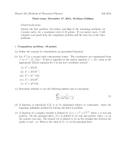
Fig. 1: An illustration of the “peeling” recovery process
on an 8 × 8 signal with 15 nonzero frequencies. In each
step, the algorithm recovers all 1-sparse columns and rows
(the recovered entries are depicted in red). The process
converges after a few steps.
The key feature of our algorithms is that their sample
complexity bounds are optimal. For the exactly sparse
case, the lower bound of Ω(k) is immediate. For the approximately sparse case, we note that the Ω(k log(n/k))
lower bound of [26] holds even if the spectrum is the sum
of a k-sparse signal vector in {0, 1, −1}n and Gaussian
noise. The latter is essentially a special case of the
distributions handled by our algorithm as shown in [9].
From the running time perspective, our algorithms are
slightly faster than those in [14], with the improvement
occurring for low values of k.
An additional feature of the first algorithm (in the table)
is its simplicity and therefore its low “big-Oh” overhead.
As a result, this algorithm is easy to adapt for practical
applications. In [28], we have customized this algorithm
and applied it to 2D Magnetic Resonance Spectroscopy
(MRS). MRS is an advanced type of medical imaging
used to detect biomarkers of diseases [4]. In this particular application, our algorithm outperformed compressive
sensing and reduced the required measurements by almost
a factor of 3x, hence reducing the overall cost and the time
the patient has to spend in the MRI machine.
B. Our Techniques
Our first algorithm for k-sparse signals is based on the
following observation: The spike-train filter (i.e., uniform
sub-sampling) is one of the most efficient ways for
mapping the Fourier coefficients into buckets. For onedimensional signals however, this filter is not amenable
to randomization. Hence, when multiple nonzero Fourier
coefficients collide into the same bucket, one cannot
efficiently resolve the collisions by randomizing the spiketrain filter. In contrast, for two-dimensional signals, we
naturally obtain two distinct spike-train filters, which
correspond to subsampling the columns and subsampling
the rows. Hence, we can resolve colliding nonzero Fourier
coefficients by alternating between these two filters.
More specifically, recall that one way to compute the
two-dimensional DFT of a signal x is to apply the onedimensional DFT to each
√ column and then to each row.
Suppose that k = a n for a < 1. In this case, the
expected number of nonzero entries in each row is less
than 1. If every row contained exactly one nonzero entry,
then the DFT could be computed via the following two
step process. In the first step, we select the first two
columns of x, denoted by u(0) and u(1) , and compute
their DFTs u
b(0) and u
b(1) . Let ji be the index of the unique
nonzero entry in the i-th row of x
b, and let a be its value.
(0)
(1)
Observe that√u
bi = a and u
bi = aω −ji (where ω is
a primitive n-th root of unity), as these are the first
two entries of the inverse Fourier transform of a 1-sparse
signal aeji . Thus, in the second step, we can retrieve
(0)
the value of the nonzero entry, equal to u
bi , as well as
(1)
(0)
the index ji from the phase of the ratio u
bi /b
ui . (this
technique was introduced in [14], [21] and was referred
to as the “OFDM trick”). The total time is dominated
by √
the cost of the two DFTs of the columns, which is
O( n log n). Since the algorithm queries only a constant
√
number of columns, its sample complexity is O( n).
In general, the distribution of the nonzero entries over
the rows can be non-uniform –i.e., some rows may have
multiple nonzero Fourier coefficients. Thus, our actual algorithm alternates the above recovery process between the
columns and rows (see Figure 1 for an illustration). Since
the OFDM trick works only on 1-sparse columns/rows,
we check the 1-sparsity of each column/row by sampling
a constant number of additional entries. We then show
that, as long as the sparsity constant a is small enough,
this process recovers all entries in a logarithmic number
steps with constant probability. The proof uses the fact
that the probability of the existence of an “obstructing
configuration” of nonzero entries which makes the process
deadlocked (e.g., see Figure 2) is upper bounded by a
small constant.
√
The algorithm is extended to the case of k = o( n)
via a reduction. Specifically,√we subsample the signal x by
the reduction ratio R = α n/k for some small enough
constant α in each dimension. The subsampled signal
↓
↓
→
↓
↓
↓
→
→
→
→
(a)
(b)
Fig. 2: Examples of obstructing sequences of nonzero
entries. None of the remaining rows or columns has a
sparsity of 1.
√
√
√
x′ has dimension m × m, where m = αk . Since
subsampling in time domain corresponds to “spectrum
folding”, i.e., adding together
all frequencies with indices
√
that are equal modulo m, the nonzero entries of x
b are
mapped into the entries of xb′ . It can be seen that, with
constant probability, the mapping is one-to-one. If this is
the case, we can use the earlier algorithm for
√ sparse DFT
m log m) =
to compute
the
nonzero
frequencies
in
O(
√
O( k log k) time, using O(k) samples. We then use the
OFDM trick to identify the positions of those frequencies.
Our second algorithm for the exactly sparse case works
for all values of k. The main idea behind it is to
decode rows/columns with higher sparsity than 1. First,
we give a deterministic, worst-case algorithm for 1dimensional sparse Fourier transforms that takes O(k 2 +
k(log log n)O(1) ) time. This algorithm uses the relationship between sparse recovery and syndrome decoding of
Reed-Solomon codes (due to [3]). Although a simple
application of the decoder yields O(n2 ) decoding time, we
show that by using appropriate numerical subroutines one
can in fact recover a k-sparse vector from O(k) samples
in time O(k 2 + k(log log n)O(1) ).4 In particular, we use
Berlekamp-Massey’s algorithm for constructing the errorlocator polynomial and Pan’s algorithm for finding its
roots. For our fast average-case, 2-dimensional sparse
Fourier transform algorithm, we fold the spectrum into
k
B = C log
k bins for some large constant C. Since the
positions of the k nonzero frequencies are random, it
follows that each bin receives t = Θ(log k) frequencies
with high probability. We then take Θ(t) samples of
the time domain signal corresponding to each bin, and
recover the frequencies corresponding to those bins in
O(t2 + t(log log n)O(1) ) time per bin, for a total time
of O(k log k + k(log log n)O(1) ).
This approach works as long as the number of nonzero
coefficients per column/row are highly √concentrated.
However, this is not the case for k ≪ n log n. We
overcome this difficulty by replacing a row by a sequence
of rows. A technical difficulty is that the process might
lead to collisions of coefficients. We resolve this issue by
using a two level procedure, where the first level returns
4 We note that, for k = o(log n), this is the fastest known worst-case
algorithm for the exactly sparse DFT.
the syndromes of colliding coefficients as opposed to the
coefficients themselves; the syndromes are then decoded
at the second level.
The above description summarizes the second algorithm. Due to space limitations, the full-description of the
second algorithm along with the proofs of the lemmas are
not included in this paper. They are available on arxiv [9].
Our third algorithm
√ works for approximately sparse
data, at sparsity Θ( n). Its general outline mimics that
of the first algorithm. Specifically, it alternates between
decoding columns and rows, assuming that they are 1sparse. The decoding subroutine itself is similar to that
of [14] and uses O(log n) samples. The subroutine first
checks whether the decoded entry is large; if not, the
spectrum is unlikely to contain any large entry, and the
subroutine terminates. The algorithm then subtracts the
decoded entry from the column and checks whether the
resulting signal contains no large entries in the spectrum
(which would be the case if the original spectrum was
approximately 1-sparse and the decoding was successful).
The check is done by sampling O(log n) coordinates and
checking whether their sum of squares is small. To prove
that this check works with high probability, we use the
fact that a collection of random rows of the Fourier matrix
is likely to satisfy the Restricted Isometry Property of [7].
A technical difficulty in the analysis of the algorithm is
that the noise accumulates in successive iterations. This
means that a 1/ logO(1) n fraction of the steps of the algorithm will fail. However, we show that the dependencies
are “local”, which means that our analysis still applies to
a vast majority of the recovered entries. We continue the
iterative decoding for log log n steps, which ensures that
all but a 1/ logO(1) n fraction of the large frequencies are
correctly recovered. To recover the remaining frequencies,
we resort to algorithms with worst-case guarantees.
C. Extensions
Our algorithms have natural extensions to dimensions
higher than 2. We do not include them in this paper as
the description and analysis are rather cumbersome.
Moreover, due to the equivalence between the twodimensional case and the one-dimensional case where n
is a product of different prime powers [11], [16], our
algorithms also give optimal sample complexity bounds
for such values of n (e.g., n = 6t ) in the average case.
II. R ELATED W ORK
As described in the introduction, the most efficient prior
algorithms for computing the sparse DFT are due to [14].
For signals that are exactly k-sparse, the first algorithm
runs in O(k log n) time. For approximately sparse signals,
the second algorithm runs in O(k log n log(n/k)) time.
Formally, the latter algorithm works for any signal x,
and computes an approximation vector x
b′ that satisfies
the ℓ2 /ℓ2 approximation guarantee, i.e., kb
x−x
b′ k2 ≤
C mink-sparse y kb
x − yk2 , where C is some approximation
factor and the minimization is over k-sparse signals. Note
that this guarantee generalizes that of Equation (1).
After this work was completed (see the arxiv version [9]), we became aware that another group has concurrently developed an efficient algorithm for the one
dimensional exactly k-sparse case where the size of the
signal n is product of primes (i.e., can be formed as a 2D
discrete Fourier transform problem) [25]. Their algorithm
is analyzed for the average case and achieves O(k) sample
complexity and runs in O(k log k). In comparison, our
algorithms achieve similar guarantees for the exactly ksparse case, but they further address the general case
where the signal is contaminated by noise.
We also mention another efficient algorithm, due
to [21], designed for the exactly k-sparse model. The
average case analysis presented in that paper also shows
that the algorithm has O(k) expected sample complexity
and runs in O(k log k) time. However, the algorithm
assumes the input signal x is specified as a function over
an interval [0, 1] that can be sampled at arbitrary positions,
as opposed to a given discrete sequence of n samples as
in our case. Thus, though very efficient, that algorithm
does not solve the Discrete Fourier Transform problem.
III. P RELIMINARIES
This section introduces the notation, assumptions and
definitions used in the rest of this paper.
√
A. Notation: Throughout the paper we assume that n is
a power of 2. We use [m] to denote the set {0, . . . , m−1},
and [m] × [m] = [m]2 to denote the m × m grid
√
{(i, j) : i ∈ [m],√
j ∈ [m]}. We define ω = e−2πi/ n
to be a primitive n-th root of unity and ω ′ = e−2πi/n
to be a primitive n-th root of unity. For any complex
number a, we use φ(a) ∈ [0, 2π)
√ to √denote the phase
of a. For a 2D matrix √
x ∈ C √n× n , its support is
denoted by supp(x) ⊆ [ n] × [ n]. We use kxk0 to
denote |supp(x)|, the number of nonzero coordinates of
x. Its 2D Fourier spectrum is denoted by x
b. Similarly, if
y is in frequency-domain, its inverse is denoted by yˇ.
B. Definitions: The paper uses the comb filter used in [17],
[15]. The filter generalizes
√ to 2√dimensions as follows:
Given
(τ
,
τ
)
∈
[
n] × [ n], and Br , Bc that dir
c
√
vide n, then for all (i, j) ∈ [Br ] × [Bc ] set yi,j =
xi(√n/Br )+τr ,j(√n/Bc )+τc Then, compute the 2D DFT yˆ
of y. Observe that yˆ is a folded version of x
ˆ:
X X
x
ˆlBr +i,mBc +j ω −τr (i+lBr )−τc (j+mBc )
yˆi,j =
√
√
] m∈[ Bn
]
l∈[ Bn
r
c
C. Distributions: In the exactly sparse case, we assume
a Bernoulli model√for the√support of x
b. This means that
for all (i, j) ∈ [ n] × [ n], Pr{(i, j) ∈ supp (b
x)} =
k/n and thus E[|supp (b
x)|] = k. We assume an unknown
predefined matrix ai,j of values in C; if x
bi,j is selected
to be nonzero, its value is set to ai,j .
In the approximately sparse case,√we√assume that the
c∗ + w
c∗ i,j
signal x
b is equal to x
b ∈ C n× n , where x
c
is the “signal” and w
b is the “noise”. In particular, x∗ is
c∗ i,j is drawn
drawn from the Bernoulli model, where x
from {0, ai,j } at random independently for each (i, j) for
c∗ )|] = k. We also
some values ai,j and with E[| supp(x
require that |ai,j | ≥ L for some parameter L. w
b is a
complex Gaussian vector with variance σ 2 in both the
real and imaginary axes independently on each coordinate;
we notate
b ∼ NC (0, σ 2 In ). We will need that
p this as w
L = Cσ n/k for a sufficiently large constant C, so that
c∗ k22 ] ≥ C E[kwk
E[kx
b 22 ].
IV. BASIC A LG . FOR THE E XACTLY S PARSE C ASE
The algorithm for the noiseless case depends on the
sparsity k where k = E[|supp (b
x)|] for a Bernoulli
distribution of the support.
√
A. Basic Exact Algorithm: k = Θ( n)
√
In this section, we focus on the regime
√ k = Θ( n).
Specifically, we will assume that k = a n for a (sufficiently small) constant a > 0.
The algorithm BASIC E XACT 2DSFFT is described as
Algorithm IV.1. The key idea is to fold the spectrum into
bins using the comb filter defined in §III and estimate
frequencies which are isolated in a bin. The algorithm
takes the FFT of a row and as a result frequencies in
the same columns will get folded into the same row
bin. It also takes the FFT of a column and consequently
frequencies in the same rows wil get folded into the same
column bin. The algorithm then uses the OFDM trick
introduced in [14] to recover the columns and rows whose
sparsity is 1. It iterates between the column bins and row
bins, subtracting the recovered frequencies and estimating
the remaining columns and rows whose sparsity is 1. An
illustration of the algorithm running on an 8×8 signal with
15 nonzero frequencies is shown in Fig. 1 in Section §I.
The algorithm also takes a constant number of extra FFTs
of columns and rows to check for collisions within a bin
and avoid errors resulting from estimating bins where
the sparsity is greater than 1. The algorithm uses three
functions:
• F OLD T O B INS . This procedure folds the spectrum
into Br ×Bc bins using the comb filter described §III.
• BASIC E ST F REQ . Given the FFT of rows or columns,
it estimates the frequency in the large bins. If there
is no collision, i.e., if there is a single nonzero
frequency in the bin, it adds this frequency to the
result w
b and subtracts its contribution to the row and
column bins.
• BASIC E XACT 2DSFFT. This performs the FFT of
the rows and columns; then iterates BASIC E ST F REQ
between the rows and columns until is recovers x
b.
Analysis of BASIC E XACT 2DSFFT: The analysis relies
on the following two lemmas which we prove in [9].
procedure F OLD T O B INS(x, Br , Bc , τr , τc )
yi,j = xi(√n/Br )+τr ,j(√n/Bc )+τc for (i, j) ∈ [Br ] ×
[Bc ],
return yb, the DFT of y
procedure BASIC E ST F REQ(b
u(T ) , vb(T ) ,T , IsCol)
w
b ← 0.
P
(τ )
Compute J = {j : τ ∈T |b
uj | > 0}.
for j ∈ J do
(1)
(0)
b←u
bj /b
uj . √
√
i ← round(φ(b) 2πn ) mod n. ⊲ φ(b) is the phase
of b.
(0)
s←u
bj .
P⊲ Test whether the row orcolumn is 1-sparse
(τ )
if
uj − sω −τ i | == 0 then
τ ∈T |b
if IsCol then ⊲ whether decoding column or row
w
bi,j ← s.
else
w
bj,i ← s.
for τ ∈ T do
(τ )
u
bj ← 0
(τ )
(τ )
vbi ← vbi − sω −τ i
return w,
b u
b(T ) , vb(T )
procedure BASIC E XACT 2DSFFT(x, k)
T ← [2c]
⊲ We set c ≥ 6
for τ ∈ T do
√
u
b(τ ) ← F OLD T O B INS(x, n,
√ 1, 0, τ ).
vb(τ ) ← F OLD T O B INS(x, 1, n, τ, 0).
zb ← 0
for t ∈ [C log n] do
⊲u
b(T ) := {b
u(τ ) : τ ∈ T }
(T ) (T )
{w,
b u
b , vb } ← BASIC E ST F REQ(b
u(T ) , vb(T ) , T,
true).
zb ← zb + w.
b
{w,
b vb(T ) , u
b(T ) } ← BASIC E ST F REQ(b
v (T ) , u
b(T ) , T,
false).
zb ← zb + w.
b
return zb
Algorithm
√ IV.1: Basic Exact 2D sparse FFT algorithm for
k = Θ( n)
Lemma 4.1: For any constant α > 0, if a > 0 is a sufficiently small constant, then assuming that all 1-sparsity
tests in the procedure BASIC E ST F REQ are correct, the
algorithm reports the correct output with probability at
least 1 − O(α).
Lemma 4.2: The probability that any 1-sparsity test
invoked by the algorithm is incorrect is at most
O(1/n(c−5)/2 ).
Theorem 4.3: For any constant
α, the algorithm BA √
SIC E XACT 2DSFFT uses O( n) samples, runs in time
√
b with probO( n log n) and returns the correct vector x
ablility at least 1 − O(α) as long as a is a small enough
constant.
Proof: From Lemma 4.1 and Lemma 4.2, the
algorithm returns the correct vector x
b with probability at
least 1 − O(α) − O(n−(c−5)/2 ) = 1 − O(α) for c > 5.
The algorithm uses only O(T
√ ) = O(1) rows and
columns of x, which yields O( n) samples. The running
time is bounded by the time needed to perform O(1) FFTs
of rows and columns (in F OLD T O B INS) procedure, and
O(log n) invocations
√ of BASIC E ST F REQ. Both components take time O( n log n).
√
B. Reduction to Basic Exact Algorithm: k = o( n)
Algorithm R EDUCE
√ E XACT 2DSFFT, which is for the
case where k = o( n), is described in Algorithm IV.2.
The key idea √
is to reduce the problem from √
the case
where k = o( n) to the case where k = Θ( n). To
do that, we subsample the √
input time domain signal x by
the reduction ratio R = a n/k for some small
√
√ enough
a. The √
subsampled signal x′ has dimension m × m,
where m = ka . This implies that the probability that
any coefficient in x
b′ is nonzero is at most R2 × k/n =
a2 /k = (a2 /k) × (k 2 /a2 )/m = k/m, since m = k 2 /a2 .
This means that we can use the algorithm BASIC N OISE LESS 2DSFFT in subsection §IV-A to recover x
b′ . Each
of the entries of x
b′ is a frequency in x
b which was folded
into x
b′ . We employ the same phase technique used in [14]
and subsection §IV-A to recover their original frequency
position in x
b.
The algorithm uses two functions:
• R EDUCE T O BASIC SFFT: This folds the spectrum
into O(k) × O(k) dimensions and performs the
reduction to BASIC E XACT 2DSFFT. Note that only
the O(k) elements of x′ which will be used in
BASIC E XACT 2DSFFT need to be computed.
• R EDUCE E XACT 2DSFFT: This invokes the reduction as well as the phase technique to recover x
b.
Analysis of R EDUCE E XACT 2DSFFT: We state the following lemma which we prove in [9].
Lemma 4.4: For any constant α, for sufficiently small
a there is a one-to-one mapping of frequency coefficients
from x
b to x
b′ with probability at least 1 − α.
Theorem 4.5: For any constant α > 0,√there exists
a constant c > 0 such that if k < c n then the
algorithm R EDUCE E XACT 2DSFFT uses O(k) samples,
runs in time O(k log k) and returns the correct vector x
b
with probablility at least 1 − α.
Proof: By Theorem 4.3 and the fact that each coefficient in x
b′ is nonzero with probability O(1/k), each invocation of the function R EDUCE T O BASIC SFFT fails with
probability at most α. By Lemma 4.4, with probability at
least 1 − α, we could recover x
b correctly if each of the
calls to R ED T O BASIC SFFT returns the correct result. By
the union bound, the algorithm R EDUCE E XACT 2DSFFT
fails with probability at most α + 3 × α = O(α).
The algorithm uses O(1) invocations of BASIC E X ACT 2DSFFT on a signal of size O(k) × O(k) in addition
procedure R EDUCE T O BASIC SFFT(x, R, τr , τc )
Define x′ij = xiR+τr ,jR+τc ⊲ With lazy evaluation
return BASIC E XACT 2DSFFT(x′ , k)
procedure
√ R EDUCE E XACT 2DSFFT(x, k)
√
R ← a k n , for some constant a < 1 such that R| n.
u
b(0,0) ← R EDUCE T O BASIC SFFT(x, R, 0, 0)
u
b(1,0) ← R EDUCE T O BASIC SFFT(x, R, 1, 0)
u
b(0,1) ← R EDUCE T O BASIC SFFT(x, R, 0, 1)
zb ← 0
L ← supp(b
u(0,0) ) ∩ supp(b
u(1,0) ) ∩ supp(b
u(0,1) )
for (ℓ, m) ∈ L do
(1,0)
(0,0)
br ← u
bℓ,m /b
uℓ,m
√
√
i ← round(φ(br ) 2πn ) mod n
(0,1)
(0,0)
bc ← u
bℓ,m /b
uℓ,m
√
√
j ← round(φ(bc ) 2πn ) mod n
(0,0)
zbij ← u
bℓ,m
return zb
Algorithm
IV.2: Exact 2D sparse FFT algorithm for k =
√
o( n)
to O(k) time to recover the support using the OFDM trick.
Noting that calculating the intersection L of supports takes
O(k) time, the stated number of samples and running time
then follow directly from Theorem 4.3.
V. A LGORITHM FOR ROBUST R ECOVERY
The algorithm for noisy recovery ROBUST 2DSFFT is
shown in Algorithm V.1. The algorithm is very similar
to the exactly sparse case. It first takes FFT of rows and
columns using F OLD T O B INS procedure. It then iterates
between the columns and rows, recovering frequencies in
bins which are 1-sparse using the ROBUST E STIMATE C OL
procedure. This procedure uses the function HIKPL O CATE S IGNAL from [14] to make the estimation of the
frequency positions robust to noise.
A. Analysis of Each Stage of Recovery
Here, we show that each step of the recovery is correct
with high probability using the following two lemmas.
The first lemma shows that with very low probability
the ROBUST E STIMATE C OL procedure generates a false
negative (misses a frequency), false positive (adds a
fake frequency) or a bad update (wrong estimate of a
frequency). The second lemma is analogus to lemma 4.2
and shows that the probability that the 1-sparse test fails
when there is noise is low. The proof of these lemmas is
long and can be found in [9].
Lemma 5.1: Consider the recovery of a column/row j
in ROBUST E STIMATE C OL, where u
b and
b are the results
√ v
of F OLD T O B INS on x
b. Let y ∈ C n denote the jth
column/row of x
b. Suppose y is drawn from a permutation
invariant distribution y = y head +y residue +y gauss , where
mini∈supp(yhead ) |yi | ≥ L, ky residue k1 < ǫL, and y gauss
procedure ROBUST E STIMATE C OL(b
u, vb, T , T ′ , IsCol,
J, Ranks)
w
b ← 0.
S ← {} ⊲ Set of changes, to be tested next round.
for j ∈ J do
continue if Ranks[(IsCol, j)] ≥ log log n.
′
i ← HIKPL OCATE S IGNAL(b
u(T ) , T ′ )
⊲ Procedure from [14]: O(log2 n) time
a ← medianτ ∈T u
bτj ω τ i .
continue if |a| < L/2
⊲ Nothing significant recovered
P
continue if τ ∈T |b
uτj − aω −τ i |2 ≥ L2 |T | /10
⊲ Bad recovery: probably not 1-sparse
b ← meanτ ∈T u
bτj ω τ i .
if IsCol then ⊲ whether decoding column or row
w
bi,j ← b.
else
w
bj,i ← b.
S ← S ∪ {i}.
Ranks[(1 − IsCol, i)] += Ranks[(IsCol, j)].
for τ ∈ T ∪ T ′ do
(τ )
(τ )
u
bj ← u
bj − bω −τ i
(τ )
(τ )
vbi ← vbi − bω −τ i
return w,
b u
b, vb, S
procedure√ROBUST 2DSFFT(x, k)
T, T ′ ⊂ [ n], |T | = |T ′ | = O(log n)
for τ ∈ T ∪ T ′ do
√
u
b(τ ) ← F OLD T O B INS(x, n,
√ 1, 0, τ ).
vb(τ ) ← F OLD T O B INS(x, 1, n, τ, 0).
zb ← 0
√
n]
R ← 1[2]×[
⊲ Rank of vertex (iscolumn, index)
√
Scol ← [ n]
⊲ Which columns to test
for t ∈ [C log n] do
{w,
b u
b, vb, Srow } ←
ROBUST E STIMATE C OL(b
u, vb, T, T ′ , true, Scol , R).
zb ← zb + w.
b
√
Srow ← [ n] if t = 0 ⊲ Try each row the first time
{w,
b vb, u
b, Scol } ←
ROBUST E STIMATE C OL(b
v, u
b, T, T ′ , false, Srow , R).
zb ← zb + w.
b
return zb
Algorithm
V.1: Robust 2D sparse FFT algorithm for k =
√
Θ( n)
√
is drawn from the n-dimensional normal distribution
NC (0, σ 2 I√n ) with standard deviation σ = ǫL/n1/4 in
each coordinate on both real and imaginary axes. We don’t
require y head , y residue , and y gauss to be independent
except for the permutation invariance of their sum.
Consider the following bad events:
head
• False negative: supp(y
) = {i} and ROBUST E S TIMATE C OL does not update coordinate i.
• False positive: ROBUST E STIMATE C OL updates
•
some coordinate i but supp(y head ) 6= {i}.
Bad update: supp(y head
{i} and coordinate i
) = head
b − y
> ky residue k1 +
is
estimated
by
b
with
i
q
log log n
log n ǫL.
For any constant c and ǫ below a small enough constant,
there exists a distribution over sets T, T ′ of size O(log n),
such that as a distribution over y and T, T ′ we have
c
• The probability of a false negative is 1/ log n.
c
• The probability of a false positive is 1/n .
c
• The probability of a bad update is 1/ log n.
m
Lemma 5.2: Let y ∈ C be drawn from a permutation
invariant distribution with r ≥ 2 nonzero values. Suppose
that all the nonzero entries of y have absolute value at
least L. Choose T ⊂ [m] uniformly at random with t :=
|T | = O(c3 log m). Then, the probability that there exists
a y ′ with ky ′ k0 ≤ 1 and
k(ˇ
y − yˇ′ )T k22 < ǫL2 t/n
c
)c−2 whenever ǫ < 1/8.
is at most c3 ( m−r
B. Analysis of Overall Recovery
Recall that we are
the recovery of a signal
√ considering
√
c∗ + w
c∗ is drawn from the
x
b = x
b ∈ C n× n , where x
√
Bernoulli model with expected k = a n nonzero entries
for a sufficiently
b ∼ NC (0, σ 2 In )
p small constant1/4a, and w
with σ = ǫL k/n = Θ(ǫL/n ) for small enough ǫ.
It will be useful to consider a bipartite graph represen√
c∗ . We construct a bipartite graph with n
tation G of x
nodes on each side, where the left side corresponds to
rows and the right side corresponds to columns. For each
c∗ ), we place an edge between left node i
(i, j) ∈ supp(x
c∗ (i,j) .
and right node j of weight x
Our algorithm is a “peeling” procedure on this graph.
It iterates over the vertices, and can with a “good probability” recover an edge if it is the only incident edge
on a vertex. Once the algorithm recovers an edge, it can
remove it from the graph. The algorithm will look at the
column vertices, then the row vertices, then repeat; these
are referred to as stages. Supposing that the algorithm
succeeds at recovery on each vertex, this gives a canonical
order to the removal of edges. Call this the ideal ordering.
In the ideal ordering, an edge e is removed based on
one of its incident vertices v. This happens after all other
edges reachable from v without passing through e are
removed. Define the rank of v to be the number of such
reachable edges, and rank(e) = rank(v) + 1 (with rank(v)
undefined if v is not used for recovery of any edge).
Lemma 5.3: Let c, α be arbitrary constants, and a a
sufficiently small constant depending on c, α. Then with
1 − α probability every component in G is a tree and at
most k/ logc n edges have rank at least log log n.
Lemma 5.4: Let ROBUST 2DSFFT’ be a modified RO BUST 2DSFFT that avoids false negatives or bad updates:
whenever a false negative or bad update would occur,
an oracle corrects the algorithm. With large constant
probability, ROBUST 2DSFFT’ recovers zb such that there
exists a (k/ logc n)-sparse zb′ satisfying
kb
z−x
b − zb′ k22 ≤ 6σ 2 n.
Furthermore, only O(k/ logc n) false negtives or bad
updates are caught by the oracle.
Lemma 5.5: For any constant α > 0, the algorithm
ROBUST 2DSFFT can with probability 1 − α recover zb
such that there exists a (k/ logc−1 n)-sparse zb′ satisfying
kb
z−x
b − zb′ k22 ≤ 6σ 2 n
using O(k log n) samples and O(k log2 n) time.
The algorithm in [14] can be generalized to the 2 dimensional case. The generalization can be found in [9]. Here,
we restate the theorem which we will use to prove the
correctness of our ROBUST 2DSFFT algorithm.
Theorem 5.6: There
√ is
√ a variant of [14] algorithm that
will, given x, zb ∈ C n× n , return xb′ with
kb
x − zb − xb′ k2 ≤ 2 ·
c∗ k22 + kb
min kb
x − zb − x
xk22 /nc
∗
c
k-sparse x
with probability 1 − α for any constants c, α > 0 in time
O(k log(n/k) log2 n + |supp(b
z )| log(n/k) log n),
using O(k log(n/k) log2 n) samples of x.
Theorem 5.7: Our overall algorithm can recover x
b′
satisfying
kb
x−x
b′ k22 ≤ 12σ 2 n + kb
xk22 /nc
with probability 1 − α for any constants c, α > 0 in
2
O(k
√ log n) samples and O(k log n) time, where k =
a n for some constant a > 0.
Proof: By Lemma 5.5, we can recover an O(k)sparse zb such that there exists an (k/ logc−1 n)-sparse zb′
with
kb
x − zb − zb′ k22 ≤ 6σ 2 n.
with arbitrarily large constant probability for any constant
c using O(k log2 n) time and O(k log n) samples. Then
by Theorem 5.6, we can recover a zb′ in O(k log2 n) time
and O(k log4−c n) samples satisfying
xk22 /nc
kb
x − zb − zb′ k22 ≤ 12σ 2 n + kb
and hence x
b′ := zb + zb′ is a good reconstruction for x
b.
R EFERENCES
[1] A. Akavia. Deterministic sparse Fourier approximation via fooling
arithmetic progressions. COLT, pages 381–393, 2010.
[2] A. Akavia, S. Goldwasser, and S. Safra. Proving hard-core
predicates using list decoding. FOCS, 44:146–159, 2003.
[3] M. Akcakaya and V. Tarokh. A frame construction and a universal
distortion bound for sparse representations. Signal Processing,
IEEE Transactions on, 56(6):2443 –2450, june 2008.
[4] O. C. Andronesi, G. S. Kim, E. Gerstner, T. Batchelor, A. A.
Tzika, V. R. Fantin, M. G. V. Heiden, and A. G. Sorensen.
Detection of 2-hydroxyglutarate in idh-mutated glioma patients
by in vivo spectral-editing and 2d correlation magnetic resonance
spectroscopy. 4:116ra4, 2012.
[5] V. Bahskarna and K. Konstantinides. Image and video compression
standards : algorithms and architectures. Kluwer Academic
Publishers, 1995.
[6] P. Boufounos, V. Cevher, A. C. Gilbert, Y. Li, and M. J. Strauss.
What’s the frequency, kenneth?: Sublinear fourier sampling off the
grid. RANDOM/APPROX, 2012.
[7] E. Candes and T. Tao. Near optimal signal recovery from
random projections: Universal encoding strategies. IEEE Trans.
on Info.Theory, 2006.
[8] Y. Chan and V. Koo. An Introduction to Synthetic Aperture Radar
(SAR). Progress In Electromagnetics Research B, 2008.
[9] B. Ghazi, H. Hassanieh, P. Indyk, D. Katabi, E. Price, and L. Shi.
Sample-Optimal Average-Case Sparse Fourier Transform in Two
Dimensions. arXiv:1303.1209, 2013.
[10] A. Gilbert, S. Guha, P. Indyk, M. Muthukrishnan, and M. Strauss.
Near-optimal sparse Fourier representations via sampling. STOC,
2002.
[11] A. Gilbert, M. Muthukrishnan, and M. Strauss. Improved time
bounds for near-optimal space Fourier representations. SPIE
Conference, Wavelets, 2005.
[12] B. G. Haskell, A. Puri, and A. N. Netravali. Digital video : an
introduction to MPEG-2. Chapman and Hall, 1997.
[13] H. Hassanieh, F. Adib, D. Katabi, and P. Indyk. Faster gps via the
sparse fourier transform. MOBICOM, 2012.
[14] H. Hassanieh, P. Indyk, D. Katabi, and E. Price. Near-optimal
algorithm for sparse Fourier transform. STOC, 2012.
[15] H. Hassanieh, P. Indyk, D. Katabi, and E. Price. Simple and
practical algorithm for sparse Fourier transform. SODA, 2012.
[16] M. Iwen. Improved approximation guarantees for sublineartime Fourier algorithms. Applied And Computational Harmonic
Analysis, 2012.
[17] M. A. Iwen. Combinatorial sublinear-time Fourier algorithms.
Foundations of Computational Mathematics, 10:303–338, 2010.
[18] M. A. Iwen, A. Gilbert, and M. Strauss. Empirical evaluation
of a sub-linear time sparse dft algorithm. Communications in
Mathematical Sciences, 5, 2007.
[19] A. Kak and M. Slaney. Principles of Computerized Tomographic
Imaging. Society for Industrial and Applied Mathematics, 2001.
[20] K. Kazimierczuk and V. YU. Accelerated nmr spectroscopy by
using compressed sensing. Angewandte Chemie International
Edition, 2011.
[21] D. Lawlor, Y. Wang, and A. Christlieb. Adaptive sub-linear time
fourier algorithms. arXiv:1207.6368, 2012.
[22] M. Lustig, D. Donoho, J. Santos, and J. Pauly. Compressed sensing
mri. Signal Processing Magazine, IEEE, 25(2):72–82, 2008.
[23] Y. Mansour. Randomized interpolation and approximation of
sparse polynomials. ICALP, 1992.
[24] D. Nishimura. Principles of Magnetic Resonance Imaging. Society
for Industrial and, 2010.
[25] S. Pawar and K. Ramchandran. Computing a k-sparse n-length
Discrete Fourier Transform using at most 4k samples and O(k log
k) complexity . In ISIT, 2013.
[26] E. Price and D. P. Woodruff. (1 + ǫ)-approximate sparse recovery.
FOCS, 2011.
[27] E. E. Schadt, M. D. Linderman, J. Sorenson, L. Lee, and G. P.
Nolan. Computational solutions to large-scale data management
and analysis. 2011.
[28] L. Shi, O. Andronesi, H. Hassanieh, B. Ghazi, D. Katabi, and
E. Adalsteinsson. MRS Sparse-FFT: Reducing Acquisition Time
and Artifacts for In Vivo 2D Correlation Spectroscopy. In
ISMRM’13, Int. Society for Magnetic Resonance in Medicine
Annual Meeting and Exhibition, 2013.
[29] E. Sidky. What does compressive sensing mean for X-ray CT
and comparisons with its MRI application. In Conference on
Mathematics of Medical Imaging, 2011.
[30] G. Wallace. The JPEG still picture compression standard. Communications of the ACM, 1991.
[31] O. Yilmaz. Seismic Data Analysis: Processing, Inversion, and Interpretation of Seismic Data. Society of Exploration Geophysicists,
2008.
[32] J. Yoo, S. Becker, M. Loh, M. Monge, E. Cand`es, and A. ENeyestanak. A 100MHz–2GHz 12.5x subNyquist rate receiver in
90nm CMOS. In IEEE RFIC, 2012.