Dealing with Packet Delay
Variation in IEEE 1588
Synchronization Using
a Sample-Mode Filter
Margaret Anyaegbu
and Cheng-Xiang Wang
Joint Research Institute for Signal and Image Processing
School of Engineering & Physical Sciences,
Heriot-Watt University Edinburgh,
EH14 4AS, UK
E-mails: {mua4, cheng-xiang.wang}@hw.ac.uk
William Berrie
TES Electronic Solutions Ltd., Research Avenue North,
Heriot-Watt University Research Park Riccarton,
Edinburgh, EH14 4AP, UK
E-mail: [email protected]
ITST 2012
© wikimedia commons & 1995 expert software
Abstract—In this paper, we characterize the delay
proﬁle of an Ethernet cross-trafﬁc network statically
loaded with one of the ITU-T network models and a
larger Ethernet inline trafﬁc loaded with uniformlysized packets, showing how the average time interval between consecutive minimum-delayed packets
increases with increased network load. We compare
three existing skew-estimation algorithms and show
that the best performance is achieved by solving a linear programming problem on “de-noised” delay samples. This skew-estimation method forms the basis of
The authors would like to acknowledge the support from the Opening Project of the Key Laboratory of Cognitive Radio and Information
Processing (Guilin University of Electronic Technology), Ministry
of Education (Grant No. 2013KF01), and the Fundamental Research
Program of Shenzhen City (Grant No.: JCYJ20120817163755061 and
JC201005250067A).
Digital Object Identifier 10.1109/MITS.2013.2267546
Date of publication: 25 October 2013
a new sample-mode algorithm for packet delay variation ﬁltering. We use numerical simulations in OPNET
to illustrate the performance of the sample-mode ﬁlter
in the networks. We compare the performance of the
proposed PDV ﬁlter with those of the existing sample
minimum, mean, and maximum ﬁlters and observe that
the sample-mode ﬁltering algorithm is able to match or
outperform other types of ﬁlters, at different levels of
network load.
I. Introduction
M
obile telecommunications operators are now
in the process of upgrading their base station backhaul networks from traditional
circuit-switched E1 links to packet-switched
networks such as Carrier Ethernet [1]–[3]. There has
also been consideration for using Digital Enhanced
Cordless Telecommunications (DECT) video systems
IEEE Intelligent transportation systems magazine •
20
• Winter 2013
1939-1390/13/$31.00©2013IEEE
connected over an Ethernet backbone in transportation
applications such as train carriages. This migration to
Ethernet has been driven by the desire to reduce installation and deployment costs, as well as the need to provide
increased bandwidth for new types of services.
Since Ethernet was not designed for the transport of
synchronization, this is an important migration consideration. Cellular systems require frequency synchronization in order to preserve connection integrity and facilitate
seamless handover, while Time Division Duplexing (TDD)
or Time Division Multiple Access (TDMA) systems need to
be synchronized in time in order to improve system capacity and reduce interference. For instance, there has been
interest in providing frame and multi-frame time synchronization for DECT base stations [4]. The authors of [5] and
[6] have also studied time synchronization in base stations
for mobile backhaul applications. For both mobile backhaul and DECT applications, the required synchronization
accuracy is in the microseconds range.
Three basic methods exist for providing precision synchronization in Ethernet networks: by means of telecoms-grade
GPS receivers deployed at each node, via the physical layer
e.g., Synchronous Ethernet (SyncE), or by exchanging timestamps using a packet protocol. The GPS solution is expensive, due to the cost of installation at each node. Additionally,
GPS receivers require a view of the sky in order to function.
SyncE [7] adds a physical-layer synchronous signal to traditional Ethernet, in order to deliver the same effect as the E1
frame. Although SyncE can deliver a high level of frequency
accuracy without susceptibility to packet delay variation
(PDV), it cannot provide time synchronization [8]. The most
popular packet-based synchronization protocols are Network
Time Protocol (NTP) [9] and IEEE 1588 Precision Time Protocol (PTP) [10]; however unlike PTP, NTP cannot deliver the
sub-microsecond synchronization accuracy required for the
DECT and mobile backhaul applications. A reserved timing
network such as the new PTP-based Ethernet Audio Video
Bridging (AVB) standard [11] can also transport synchronous
information; however our goal is to provide time synchronization on a legacy network without reservation.
When PTP is deployed in a network, the synchronization
traffic must contend for the network path and share existing network elements with the non-synchronization traffic.
This contention causes PDV at the output queue buffers of
network switches, which can adversely affect the synchronization accuracy. The PTP standard recognizes this issue and
offers some recommendations for dealing with PDV, such
as deploying PTP transparent clocks or boundary clocks at
intermediate nodes in the network, trafﬁc design, priority
tagging of synchronization trafﬁc, and PDV ﬁltering. Other
techniques in the literature deal with PDV by coordinating
the background trafﬁc packet departures with the synchronisation packet generation so as to completely eliminate PDV
[12], or by applying Kalman ﬁltering to the received synchro-
nization packets in order to estimate the master time [13],
[14]. This paper, however, focuses on PDV ﬁltering.
In general, the goal of PDV ﬁltering is to select at least
one “good” packet out of the received synchronization
trafﬁc and then use these packets to achieve synchronization. For most of the PDV ﬁltering algorithms in the literature [15]–[17], a “good” packet has been deﬁned as one with
the shortest transit time through the network.
These sample-minimum ﬁltering algorithms can work
effectively, as long as packets with minimal queuing delay
are delivered at appropriate intervals. In [18], [19], the
authors show that this is true for cross-trafﬁc networks
with moderate levels of background trafﬁc (less than 45%
utilization). However, they observed that for a heavilyloaded cross-trafﬁc network and moderately-loaded highhop in-line trafﬁc network, the probability of ﬁnding a
minimum-delay packet was reduced. They thus proposed
sample-mean and sample-maximum ﬁlters based on the
observed delay distributions in the networks.
In this paper, we characterize the delay distributions
of a cross-trafﬁc network at different network load levels
and illustrate how the time interval between consecutive
minimum-delayed packets increases with the network load.
We further consider the delay distribution of a large in-line
trafﬁc network. For observed delay distributions, we suggest
the type of existing ﬁlter that performs best. Then, we consider three existing skew-estimation algorithms and compare their performance with a new skew-estimation algorithm that uses features from two existing algorithms. This
algorithm forms the basis of a new iterative sample-mode
PDV ﬁltering technique that ﬁlters packets via a mode bin
to achieve synchronization. Finally, we compare the performance of this sample mode ﬁlter with existing ﬁlters for the
network scenarios whose delay distributions were proﬁled.
Section II of this paper deﬁnes some clock terminology
and describes how the performance of PDV ﬁltering algorithms can be impacted by the delay proﬁle of a network.
In Section III, the existing approaches to PDV ﬁltering are
summarized, while the proposed sample-mode ﬁltering
algorithm is described in Section IV. Simulation results
and analysis are presented in Section V. Finally, conclusions are drawn in Section VI.
II. Characterizing Packet Delays
In this section, we consider how network queuing delays
give rise to PDV and how the delays can be proﬁled using
Probability Distribution Functions (PDFs). But ﬁrst of all,
we introduce some of the terminology commonly used to
describe clock behavior.
A. Clock Terminology
Mathematically, a clock C ^ t h is a piecewise continuous
function of t that is twice differentiable except on a ﬁnite
set of isolated jump points where the clock is reset [20], [21].
IEEE Intelligent transportation systems magazine •
21
• Winter 2013
Switch_1
skew, then d i will also include an accumulated offset, as shown in (1).
Switch_2 Switch_3 Switch_4 Switch_5
Timing Master
(1)
This accumulated offset (M i + d i) v causes
d i to gradually increase or decrease over
time, depending on whether the slave
clock runs faster or slower than the master clock.
Timing Slave
Station_1
d i = d i + (M i + d i) v. Station_2 Station_3 Station_4 Station_5
C. Packet Delay Proﬁling
Synchronization Traffic
Background Traffic
Fig 1 5-hop network topology for cross trafﬁc.
A perfect clock or “true” clock runs at a constant rate of unity
and reports the “true” time at any time. For a “true” clock C t,
C t ^ t h = t.
Real clocks do not report “true” time. Given two real clocks
C a and C b, we can deﬁne a clock’s offset as the instantaneous
difference between the clock’s reading and “true” time. The
offset of C a is ^C a ^ t h - t h, while the relative offset of clock
C b with respect to C a at time t $ 0 is C b ^ t h - C a ^ t h . Clock
frequency refers to the rate at which the clock progresses.
The frequency of C a at time t is C la (t) . If C la (t) > 1, then
C a runs faster than the “true” clock C t; else if C la (t) < 1,
then C a runs slower than C t . Clock skew is the difference
in the frequencies of a real clock and the “true” clock. The
skew of C a is (C la (t) - 1), while the relative skew of clock
C b with respect to C a is C a is (C lb (t) - C la (t)) . Lastly, clock
drift is deﬁned as the rate at which the frequency of a clock
changes, often due to temperature variation or oscillator
aging. The drift of C a is C lla (t) . In this paper, we denote a
clock’s frequency as n and a clock’s skew as v.
B. Packet Delay Variation
In the PTP protocol, the master node multicasts a 44 byte
SYNC packet to the slaves every synchronization interval.
The SYNC packet includes the master’s origin timestamp
M i and each slave records the time S i at which it received
the i th SYNC packet. The end-to-end delay experienced by
each packet is given by:
d i = d trans + d prop + d queue .
i
Since the packet size is ﬁxed for all SYNC packets, the
transmission delay d trans is constant and if the packets follow the same route to the slave, the propagation delay d prop
will also be constant. It is the variable queuing delay d queue
that gives rise to PDV.
If the slave clock is perfectly synchronized to the master,
the difference between the two timestamps for each SYNC
packet d i = S i - M i will be equal to the end-to-end delay
d i experienced by each packet. If the clocks have a non-zero
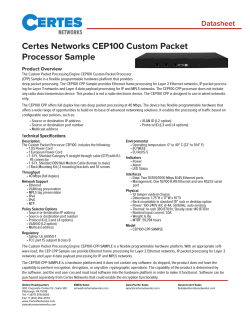
In order to characterize the delay proﬁle
and appreciate the effects of PDV on the
synchronization performance of the network, we simulated a 5 hop network with
data-centric background trafﬁc based on the ITU-T G.8261
Network Trafﬁc Model 2 [22], as illustrated in Fig. 1.
Each node generates background trafﬁc that follows the
same path as the SYNC packets. The next node extracts
the background trafﬁc and injects new (independent)
trafﬁc along the synchronization path. In the literature,
this type of trafﬁc pattern is referred to as cross-trafﬁc
[19]. Quality of Service (QoS) was implemented in the
model so that the SYNC packets were transmitted with
strict priority queuing at the switch output ports. Simulations were carried out for 20%, 40%, 60% and 80% background trafﬁc load levels. Other simulation parameters
are provided in Table 1.
For each SYNC packet received at the slave, the end-toend delay was measured and used to generate an experimental PDF of the packet delay, as shown in Fig. 2. At low
loads (typically less than 45%), most of the packets experienced no queuing in the network, as evidenced by the
very strong modes at the minimum delay value. As the load
increases, the probability of ﬁnding a packet with minimum delay decreases. For example, Fig. 3 shows that there
is no packet at the minimum delay value at 70% load, as all
the packets experience queuing in the network. In fact, the
PDFs at higher loads have well-deﬁned shapes and can be
ﬁtted to Erlang density distributions.
Inspection of the delay proﬁles in Fig. 2 suggests that
the low load scenarios are amenable to sample-minimum
ﬁltering, while the higher load scenarios might beneﬁt
from sample-mean ﬁltering.
We also consider the network scenario depicted by
Fig. 4, where the background trafﬁc follows the same
Table 1. Simulation parameters for packet delay profiling.
i
Distance
Between
Nodes
Synchronization
Interval
Fractional
Frequency
Offset of Slave
Line Rate
50 metres
3.90625 milliseconds
2 parts per million
100 Mbps
IEEE Intelligent transportation systems magazine •
22
• Winter 2013
0.02
80% Load—Experimental
80% Load—Theoretical, Erlang (0.0309, 9)
60% Load—Experimental
60% Load—Theoretical, Erlang (0.0214, 5)
40% Load—Experimental
20% Load—Experimental
0.018
0.016
0.014
PDF
0.012
0.01
0.008
0.006
0.004
0.002
0
0
100
600
700
3.5
3
2.5
2
1.5
1
0.5
0
0
10
III. Existing Packet Filtering Techniques
As previously mentioned, the performance of a PDV ﬁlter
depends on the probability of ﬁnding “good” packets among
a sequence of arriving packets within a window. Thus the
aim of PDV ﬁltering is to select packets that experienced
similar amount of delay through the network. If the distribution of the delay is known a-priori, then the best ﬁlter to
use is the one which matches the delay distribution, thus
maximizing the chances of ﬁnding good packets. However,
if the delay distribution does not quite match up with any of
the ﬁlters, then the residual clock offset after synchronization might be greater than desired.
Three main types of ﬁlters have been considered for
PDV ﬁltering, namely sample minimum, sample maximum
and sample mean.
Given a window with W SYNC packets, master origin
timestamp M i, slave reception timestamp S i, and delay
d i = S i - M i for the i th packet (0 1 i # W ), good packets
are deﬁned as those that satisfy (2) for a sample-minimum
ﬁlter [15]–[17], (3) for a sample-maximum ﬁlter, and (4)
for a sample-mean ﬁlter [19]; where d min, d max, and d mean
are the minimum, maximum, and mean, respectively, of
200 300 400 500
Sync Packet Delay (ns)
Fig 2 Packet delay distribution for a 5-hop cross trafﬁc network.
Average Interval between Fastest
Packets (s)
path as the synchronization trafﬁc. This type of trafﬁc,
termed in-line trafﬁc, has practical significance in access
aggregation networks such as in mobile backhaul systems
where a network controller provides both timing trafﬁc
and background trafﬁc (such as voice and data) to base
stations. We modelled a 16-hop network in which the size
of the packets was uniformly distributed between 64 bytes
and 1500 bytes, which are the minimum and maximum
packet sizes for Ethernet, respectively. The other simulation parameters were unchanged.
We observed that at 20% load level, the delay PDFs in
this network can again be ﬁtted to a theoretical Erlang
PDFs, as depicted in Fig. 5; however, none of the packets
experienced the minimum delay due to the long chain of
queuing elements in the network. As the load increases,
most of the packets tend to experience the maximum
amount of delay. The resulting PDFs for these increasedcongestion scenarios do not ﬁt any popular distributions,
but rather resemble mirror-images of the Erlang density
distribution with negative values of the shape parameter.
Since the delay distributions at higher loads and for
higher hop counts tend to follow an Erlang distribution,
then in theory, an optimal PDV ﬁlter can be designed
based on the Erlang distribution parameters. However, the
expected computational overhead of such a ﬁlter would
make it unsuitable for real-time use.
Inspection of the shapes of the delay proﬁles in Fig. 5
suggests that none of the scenarios would also be amenable
to sample-minimum ﬁltering. Sample-maximum ﬁltering
might beneﬁt the 80% load scenario, while the other load
scenarios might beneﬁt from sample-mean ﬁltering.
20
30
40
50
Network Load (%)
60
70
Fig 3 Average interval between minimum-delayed packets for 5-hop
cross trafﬁc network topology.
all W d i samples in the window, and the threshold value a
depends on the desired accuracy.
d i # d min + a. (2)
d i $ d max - a. (3)
(d mean - a/2) # d i # (d mean + a/2) . (4)
IV. Proposed Packet Filtering Approach
The goal of our proposed sample-mode PDV ﬁlter is to
maximize the chances of ﬁnding good packets by selecting
packets from within the mode bin. The rationale behind
this approach is that when the delay distribution does not
quite match up with any of the existing ﬁlters, the sample
mode will yield the largest number of good packets. Thus
the sample mode ﬁlter should give a good ﬁt for all trafﬁc
distributions, with a relatively low computational overhead.
IEEE Intelligent transportation systems magazine •
23
• Winter 2013
Switch_1
Switch_2
Switch_16
Timing Master
Timing Slave
Station_1
Station_2
Synchronization Traffic
Background Traffic
Fig 4 16-hop network topology for in-line trafﬁc.
5
4.5
4
f=
80% Load—Experimental
80% Load—Theoretical, Erlang (0.022, -6)
60% Load—Experimental
60% Load—Theoretical, Erlang (0.015, -7)
40% Load—Experimental
40% Load—Theoretical, Erlang (0.01, -6)
20% Load—Experimental
20% Load—Theoretical, Erlang (0.011, 14)
# 10-3
slave with respect to the master clock. After the
ﬁrst computation of the RCF, subsequent computations are done for every frequency synchronization interval, rather than for every iteration.
This is due to the well-known fact that changes
in clock rates are usually caused by aging of the
oscillators or temperature changes, and as such
they tend to occur extremely slowly. In fact, if the
maximum clock drift rate t is known, then the
frequency synchronization interval f can be
estimated from the target synchronization accuracy h as follows:
PDF
2.5
2
1.5
1
0.5
0
0
500
1000
1500
Sync Packet Delay (ns)
2000
Fig 5 Packet delay distribution for a 16-hop inline trafﬁc network.
For each SYNC packet received at the slave, d = S - M
is computed from the master origin and slave reception timestamps and stored. After W samples have been
obtained, a histogram is created to approximate the delay
distribution of the received packets. If two or more bins
have the same number of samples, the mode bin is selected
as the bin with the minimum delay value. Good packets are
deﬁned as packets selected from within the mode bin, i.e.,
(d mode - a/2) # d i # (d mode + a/2) ,
(5)
where d mode is the sample mode and a represents the
width of each histogram bin.
A. Skew Correction
The ﬁrst step in our sample mode PDV ﬁlter algorithm is
the computation of the rate compensation factor (RCF).
This RCF is used to correct for the relative clock skew at the
.
(6)
In our previous work [23], we showed that the RCF could
be calculated using the largest origin timestamp M max,
least origin timestamp M min, largest reception timestamp
S max, and least reception timestamp S min within the mode
bin as follows:
RCF =
3.5
3
h
2t
S max - S min
.
M max - M min
(7)
For an accurate computation of RCF using (7), the packets received by the slave at timestamps S max and S min must
have experienced the same delay in the network. In Appendix A, we prove that it is possible for packets that experience
different delays to end up in the same bin. If this happens
within the mode bin, the RCF computed using (7) may not
accurately reﬂect the actual amount of skew between the
master and slave. Conversely, it is also possible for packets
that experience the same delay to end up in different bins,
as shown in Appendix B. If similarly-delayed packets are
in separate bins, then it might be better to utilise all the
samples within a window when computing the RCF, rather
than selected samples from the mode bin. Thus, we have
explored other algorithms for correcting the skew.
1) Paxson’s Algorithm
Paxson’s algorithm [24], [25] was designed to remove clock
skew from a set of path delay measurements. The W d i are
partitioned into W segments, and the minimum delay
measurement from each segment is selected. The selected
measurements are referred to as the “de-noised” one-way
transit times (OTTs). The slopes of all possible pairs of the
“de-noised” OTTs are computed, and the median slope
is selected. If the median slope is negative, the algorithm
assumes that the skew is negative. On the other hand, if
the median slope is positive, a positive skew is assumed. A
cumulative minima test is then performed to see if the number of cumulative minima is large enough to indicate that
the sign of the skew is probabilistically likely. If the test is
successful, the median slope is output as the skew estimate;
otherwise the algorithm outputs a skew of zero.
IEEE Intelligent transportation systems magazine •
24
• Winter 2013
Appendix A. Proof That Packets with Different
Delays Can End Up in the Same Bin
i
1
t r is actually an estiof being greater than min i d r . Thus, d
t r is actumate of (d r + min i d r and (K
di - P
M i (nt - 1) + d
ally the variable portion of the end-to-end delay or the PDV.
Hence, the linear programming algorithm tries to minimize the sum of the PDV.
i
The standard linear regression technique can also be used
for ﬁtting a line to the set of K
M i values. For skew estid i and P
mation, the linear regression algorithm computes estimates
t r that minimize the mean square error e in
of n and d
1
2) Linear Programming
The method of [20] can be used to formulate a linear programming problem from (1). Assuming that K
d i = di - d1
and P
M i = M i - M 1 then from (1) we have
K
d i = (d i - d 1) (1 + v) + P
M i v.
(8)
Using the relation n = 1 + v, (8) can be re-written as
(9)
where d r = nd i represents the end-to-end delay of the i th
packet measured at the slave. From (9), K
d i differs from d r
by P
M i (n - 1) minus a constant d r . If n 2 1, P
M i (n - 1)
grows linearly with P
M i and K
d i gets larger. If n
t is the estit r and dt r are the estimates of d r
mate of n or RCF and d
and d r , respectively, then from (9) we can obtain
i
i
1
i
1
1
t r = Kd i - P
t r .
d
M i (nt - 1) + d
i
1
(10)
M i . Since the delay
d i and P
The goal is to estimate n, given K
t r must always be positive, the linear programming probd
lem can be formulated as
i
2
1
(13)
B. Offset Correction
a 1 nfv. (S4)
i
W
i =1
For the two packets to end up in different bins, the difference in
their d values must be greater than the bin width a, i.e.,
1
M i (nt - 1) + dt r . . / $Kd i - P
d i + n - d i = nfv. (S3)
i
1
3) Linear Regression
Again consider the i th and j th SYNC packets received within the
same window, where j - i = n and n > 0. In this case, the endto-end delay is d i = d j = d. From (1), the corresponding timestamp differences are given by d i = d + (M i + d ) v and
d j = d + (M j + d ) v, respectively. Assuming no packet loss and
equal synchronisation interval f, M i + n = M i + nf. Subtracting d i
from d j with substitution and simplification yields
K
d i = (d r - d r ) + P
M i (n - 1) ,
1
i
1
Appendix B. Proof That Packets with the Same
Delay Can End Up in Different Bins
(12)
1
1
a $ (d i + n - d i )(1 + v) + nfv. (S2)
W
t r are obtained,
It is important to note that once nt and d
the resulting estimated end-to-end delay of d r calculated
t r will be greater than zero, instead
as (K
di - P
M i (nt - 1) + d
For the two packets to end up in the same bin, the difference in
their d values must be within the bin width a, i.e.,
min ) / ^K
d i -P
M i (nt - 1) + dt r h3 . i =1
d i + n - d i = (d i + n - d i )(1 + v) + nfv. (S1)
(11)
1
The corresponding objective function is stated as
Consider the i th and j th SYNC packets received within the same
window, where j - i = n and n > 0. From (1), the corresponding
timestamp differences are given by d i = d i + (M i + d i ) v and
d j = d j + (M j + d j ) v, respectively. Assuming no packet loss and
equal synchronisation interval f, M i + n = M i + nf. Subtracting d i
from d j with substitution and simplification yields
K
t r $ 0, 1 # i # W. di - P
M i (nt - 1) + d
Once the RCF has been computed, subsequent iterations of
the algorithm aim to reduce the clock offset between the
master and the slave. At least one good packet is required
for the offset computation. The packet selection rate is
computed as the quotient of the number of packets in the
mode bin and the window size W, and then compared with
a packet selection threshold. If the selection rate exceeds
the threshold level, the window size can be reduced. On
the other hand, if no packet is found within the mode bin
after increasing the window size to the maximum, the
slave sends a management message to halve the synchronization interval at the master.
V. Simulation and Results
To determine the best skew-estimation algorithm, we used
OPNET Modeler 16.0 [26] to simulate the 5-hop cross trafﬁc
network depicted in Fig. 1. The synchronization interval
was set to 976.5625 ns, the window size was set to 10000
samples. The slave skew was ﬁxed at 2 parts per million
while the master skew was ﬁxed at 0 parts per million. The
three skew-estimation algorithms previously described
were implemented, for different levels of network load.
Additionally, we consider a new “de-noised” linear programming algorithm which applies the linear progamming algorithm described in [20] to Paxson’s [24], [25]
“de-noised” delay samples.
Fig. 6 shows the residual error after RCF estimation,
using the different algorithms. The linear regression algorithm gives unpredictable results because it is not robust in
IEEE Intelligent transportation systems magazine •
25
• Winter 2013
# 10-6
5
4
3.5
70
Relative Clock Offset (ns)
4.5
RCF Estimation Error
80
Linear Programming
Paxson Algorithm
Linear Regression
De-Noised Linear Programming
3
2.5
2
1.5
1
40
30
20
10
-10
0
10
20
30
40
50
Network Load (%)
60
70
Fig 6 RCF estimation error for 5-hop cross trafﬁc network.
20
10
0
Sample Maximum
Sample Mean
Sample Minimum
Sample Mode
-10
-20
-30
-40
-50
6
8
10
12
14
16
Simulation Time (s)
16
18
20
22
24
Simulation Time (s)
26
28
Fig 8 Relative clock offset for 16-hop inline trafﬁc network at 80% load.
30
Relative Clock Offset (ns)
Sample Maximum
Sample Mean
Sample Minimum
Sample Mode
50
0
0.5
0
60
18
20
Fig 7 Relative clock offset for 5-hop cross trafﬁc network at 40% load.
the presence of outliers. Furthermore, it is only optimal in
the mean square sense if the network delays have a normal
distribution. Paxson’s algorithm is accurate at low levels of
load, where it is possible to ﬁnd minimum-delayed packets. Since the linear programming objective function aims
to minimize the sum of the variable delays, the algorithm
works well for low levels of PDV. Combining linear programming with “de-noising” yields the best performance,
since “de-noising” gets rid of excess PDV.
We also compared the performance of the proposed
sample-mode with those of the existing ﬁlters, by simulating the networks depicted in Fig. 1 and Fig. 4. In order
to allow a like-for-like comparison of the ﬁlters, we ﬁxed
the window size at 500 samples for all ﬁlters, the threshold value a was set at 0.2 ns, the synchronization interval was 976.5625 ns and the residual fractional frequency
offset at the slave after the initial RCF estimation was 30
parts per billion.
In Fig. 7, we compare the results obtained from the
four different ﬁlters after synchronization in a 40% 5-hop
cross-trafﬁc scenario. As observed in the corresponding
delay proﬁle of Fig. 2, most of the packets experience the
minimum delay; hence the sample-minimum ﬁlter is a good
match and performs optimally. Since the mode corresponds
to the minimum delay point, the performance of our sample
mode ﬁlter is also optimal, and is in fact identical to that
of the sample-minimum. As expected, the sample-mean
and sample-maximum ﬁlters perform poorly, because they
struggle to ﬁnd “good” packets.
In Fig. 8, we compare the results obtained after synchronization in an 80% 16-hop inline-trafﬁc scenario. As observed
in the corresponding delay proﬁle of Fig. 5, none of the packets
experience the minimum delay; hence the sample-minimum
ﬁlter has the worst performance. The delay proﬁle does not
match well with the sample-mean or sample-maximum ﬁlters
either, hence their performance is also sub-optimal. Thus, the
sample-mode ﬁlter gives the best performance.
As a ﬁnal analysis, we can observe the performance
of a speciﬁc ﬁlter in both of these scenarios and see how
the performance is inﬂuenced by the corresponding delay
proﬁle. The sample-maximum ﬁlter, for example, yields
the worst performance in the ﬁrst scenario, as most packets experience the minimum delay. On the other hand,
it performs better than both the sample-minimum and
sample-mean ﬁlters in the larger heavier-loaded network
scenario which has higher levels of queuing. The converse
is true for the sample-minimum ﬁlter.
VI. Conclusions
We have characterized the IEEE 1588 PTP synchronization packet delay proﬁles for a small cross-trafﬁc network
and a large in-line trafﬁc network with different levels
of background trafﬁc and observed from the shape of the
IEEE Intelligent transportation systems magazine •
26
• Winter 2013
distributions that the existing sample-minimum, samplemaximum, and sample-mean ﬁlters perform sub-optimally
for some of the load levels in these scenarios. A new skewestimation algorithm has been proposed, by utilizing some
features of two existing algorithms. This skew-estimation
algorithm forms the basis of a low-computation samplemode ﬁltering algorithm which selects packets from the
mode bin and uses these “good” packets to achieve synchronization. Numerical simulations have shown that when the
delay proﬁle is a good match for an existing ﬁlter, the sample-mode ﬁlter performs as well as the existing ﬁlter. When
the delay proﬁle is not a good match for an existing ﬁlter, the
sample-mode ﬁlter outperforms the existing ﬁlters.
About the Authors
Margaret Anyaegbu ([email protected])
received her B.Eng. in Electronic Engineering from the University of Nigeria
in 2003, and her M.Sc.(Eng.) in Wireless
Communications from the University of
Leeds in 2006. She worked brieﬂy as a
telecommunications consultant before
embarking on an EngD degree at Heriot Watt University,
Edinburgh. Her research interest is focused on synchronisation in short-range wireless communications systems.
Cheng-Xiang Wang [S’01-M’05-SM’08]
([email protected]) received
his Ph.D. degree from Aalborg University, Denmark, in 2004. He joined
Heriot-Watt University, U.K., as a lecturer in 2005 and became a professor
in August 2011. His research interests
include wireless channel modeling and 5G wireless communication networks. He served or is serving as an editor
or guest editor for 11 international journals including IEEE
Transactions on Vehicular Technology (2011-), IEEE Transactions on Wireless Communications (2007-2009), and
IEEE Journal on Selected Areas in Communications. He has
edited one book and published one book chapter and over
180 papers in journals and conferences. He received the
Best Paper Awards from IEEE Globecom 2010, IEEE ICCT
2011, and ITST 2012.
William Berrie ([email protected]) was born in Glasgow, UK in
1958. He received the B.Sc. degree in
mathematical physics from the University of Edinburgh in 1980. He has
been awarded CEng status by the BCS.
Since 1981 he has been working in
the ﬁeld of telecommunications and since 2006 has been
working on short range wireless systems for TES Electronic Solutions Ltd.
References
[1] A. Sutton, “Building better backhaul,” Eng. Technol. Mag., vol. 6, no. 5,
pp. 72–75, June 2011.
[2] M. Howard, “Using carrier Ethernet to backhaul LTE,” White Paper,
Infonetics Research, Campbell, CA, Feb. 2011.
[3] P. Briggs, R. Chundury, and J. Olsson, “Carrier Ethernet for mobile
backhaul,” IEEE Commun. Mag., vol. 48, no. 10, pp. 94–100, Oct. 2010.
[4] C. Na, D. Obradovic, and R. Scheiterer, “Method for synchronizing clocks
in a communication network,” U.S. Patent 20 110 161 524, Sept. 2, 2008.
[5] A. Magee, “Synchronization in next-generation mobile backhaul networks,” IEEE Commun. Mag., vol. 48, no. 10, pp. 110–116, Oct. 2010.
[6] Z. Ghebretensae, J. Harmatos, and K. Gustafsson, “Mobile broadband
backhaul network migration from TDM to carrier Ethernet,” IEEE
Commun. Mag., vol. 48, no. 10, pp. 102–109, Oct. 2010.
[7] Timing Characteristics of a Synchronous Ethernet Equipment Slave
Clock, Recommendation G.8262/Y.1362, ITU-T, June 2010.
[8] J.-L. Ferrant, M. Gilson, S. Jobert, M. Mayer, M. Ouellette, L. Montini, S. Rodrigues, and S. Ruffini, “Synchronous Ethernet: A method to
transport synchronization,” IEEE Commun. Mag., vol. 46, no. 9, pp.
126–134, Sept. 2008.
[9] D. Mills, J. Martin, J. Burbank, and W. Kasch, “Network Time Protocol
(version 4) protocols and algorithms specification,” RFC 5905, June
2010.
[10] IEEE Standard for a Precision Clock Synchronization Protocol for Networked Measurement and Control Systems, IEEE Standard 1588, 2008.
[11] Timing and Synchronization for a Time-Sensitive Applications in
Bridged Local Area Networks, IEEE Standard 802.1AS, 2011.
[12] B. Mochizuki and I. Hadzic, “Improving IEEE 1588v2 clock performance through controlled packet departures,” IEEE Commun. Lett.,
vol. 14, no. 5, pp. 459–461, May 2010.
[13] C. Na, R. L. Scheiterer, D. Obradovic, and J. A. Nossek, “A Kalman filter approach to clock synchronization of cascaded network elements,”
in Proc. First IFAC Workshop Estimation Control Networked Systems,
Venice, Italy, Sept. 2009, pp. 54–59.
[14] H. Abubakari and S. Sastry, “IEEE 1588 style synchronization over
wireless link,” in Proc. IEEE Int. Symp. Precision Clock Synchronization for Measurement, Control Communication, Ann Arbor, MI, Sept.
2008, pp. 127–130.
[15] D. T. Bui, A. Dupas, and M. L. Pallec, “Packet delay variation management for a better IEEE 1588v2 performance,” in Proc. IEEE Int.Symp.
Precision Clock Synchronization Measurement, Control Communication, Brescia, Italy, Oct. 2009, pp. 75–80.
[16] T. Murakami and Y. Horiuchi, “Improvement of synchronization accuracy in IEEE 1588 using a queuing estimation method,” in Proc. IEEE
Int. Symp. Precision Clock Synchronization Measurement, Control
Communication, Brescia, Italy, Oct. 2009, pp. 12–16.
[17] S. Johannessen, “Time synchronization in a local area network,” IEEE
Control Systems Mag., vol. 24, no. 2, pp. 61–69, Apr. 2004.
[18] I. Hadzic and D. R. Morgan, “On packet selection criteria for clock recovery,” in Proc. IEEE Int. Symp. Precision Clock Synchronization Measurement, Control Communication, Brescia, Italy, Oct. 2009, pp. 35–40.
[19] I. Hadzic and D. R. Morgan, “Adaptive packet selection for clock recovery,” in Proc. IEEE Int. Symp. Precision Clock Synchronization Measurement, Control Communication, Portsmouth, NH, Sept. 2010, pp. 42–47.
[20]S. B. Moon, P. Skelly, and D. Towsley, “Estimation and Removal of clock
skew from network delay measurements,” in Proc. IEEE 18th Annu.
Joint Conf. Computer Communications Societies, New York, Mar. 1999,
vol. 1, pp. 227–234.
[21] L. Lamport, “Time, clocks and the ordering of events in a distributed
system,” Commun. ACM, vol. 21, no. 7, pp. 558–565, July 1978.
[22]Timing and Synchronization Aspects in Packet Networks, Recommendation G.8261, ITU-T, Apr. 2008.
[23]M. Anyaegbu, C.-X. Wang, and W. Berrie, “A sample-mode packet delay variation filter for IEEE 1588 synchronization,” in Proc. IEEE Int.
Conf. ITS Telecommunications, Taipei, Taiwan, Nov. 2012, pp. 1–6.
[24]V. Paxson. (1997, Apr.). Measurements and analysis of end-to-end internet dynamics. Ph.D. dissertation, Univ. California, Berkeley, CA.
[Online]. Available: ftp://ftp.ee.lbl.gov/papers/vp-thesis
[25]V. Paxson, “On calibrating measurements of packet transit times,” in
Proc. SIGMETRICS, Madison, WI, June 1998, pp. 11–21.
[26]OPNET Modeler Documentation Set, OPNET Technologies Inc.,
Bethesda, MD, 2011.
IEEE Intelligent transportation systems magazine •
27
• Winter 2013