1. art and entertainment
2. visual art and design
3. design

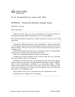
Hindawi Publishing Corporation
EURASIP Journal on Bioinformatics and Systems Biology
Volume 2008, Article ID 297945, 8 pages
doi:10.1155/2008/297945
Research Article
Which Is Better: Holdout or Full-Sample Classifier Design?
Marcel Brun,1 Qian Xu,2 and Edward R. Dougherty1, 2
1 Computational
2 Department
Biology Division, Translational Genomics Research Institute, Phoenix, AZ 85004, USA
of Electrical and Computer Engineering, Texas A&M University, College Station, TX 77843, USA
Correspondence should be addressed to Edward R. Dougherty, [email protected]
Received 26 March 2007; Revised 17 September 2007; Accepted 2 December 2007
Recommended by Yufei Huang
Is it better to design a classifier and estimate its error on the full sample or to design a classifier on a training subset and estimate its
error on the holdout test subset? Full-sample design provides the better classifier; nevertheless, one might choose holdout with the
hope of better error estimation. A conservative criterion to decide the best course is to aim at a classifier whose error is less than a
given bound. Then the choice between full-sample and holdout designs depends on which possesses the smaller expected bound.
Using this criterion, we examine the choice between holdout and several full-sample error estimators using covariance models
and a patient-data model. Full-sample design consistently outperforms holdout design. The relation between the two designs is
revealed via a decomposition of the expected bound into the sum of the expected true error and the expected conditional standard
deviation of the true error.
Copyright © 2008 Marcel Brun et al. This is an open access article distributed under the Creative Commons Attribution License,
which permits unrestricted use, distribution, and reproduction in any medium, provided the original work is properly cited.
1. Introduction
In most microarray-based classification studies, the number
of data points (microarrays) is very small (under 100) and
one has no choice but to use the full cohort of data for both
training and testing (error estimation). One must choose
among error estimators for which the full sample is used
for training. In small-sample situations, these estimators
usually suffer from either low bias (resubstitution) or high
variance (cross-validation) [1, 2]. Studies indicate that either
bootstrap [3] or bolstering [4] tend to provide better
estimation. But what happens when samples sizes are not
so small, a situation that will become more common as
technology improves? Then, rather than using full-sample
design and estimation, one has the option of holding out data
from the design and using the holdout data for estimating
the error of the classifier designed on the data not held
out.
Based upon colloquial discussions, it appears that some
people prefer to hold out data except for very small samples,
thereby splitting the sample into training and testing data;
however, these discussions usually lack any precise statistical
justification. On the other hand, when discussing holding
out test data to estimate the error of a designed classifier,
Devroye et al. state [5], “A serious problem concerning the
practical applicability of the [hold-out] estimate introduced
above is that it requires a large, independent testing sequence.
In practice, however, an additional sample is rarely available.
One usually wants to incorporate all available [sample
points] (Xi , Yi ) pairs in the decision function.” When
made by premier pattern-recognition researchers such as L.
Devroye, L. Gyorfi, and G. Lugosi, such a statement should
give pause to anyone taking a counter position. The holdout
issue arises because, even though we are assured of a smaller
true error using full-sample design, we desire a satisfactory
estimate of the error. The salient word in the Devroye et al.
quote [5] is “rarely.” Reasoning in a hyperbolic extreme, if
there were an infinite amount of data, it could be split into
infinite training and test data sets and this would constitute
one of the rare cases. But why do so? For many popular fullsample error estimators, the mean-square error between the
estimated and true errors goes to 0 as the sample size tends
to infinity. For instance, for the histogram rule with q cells,
the resubstitution estimator is low biased; nevertheless, it
εn − εn |2 ] ≤ 6q/n, where εn and εn are
satisfies the bound E[|
the estimated and true errors, respectively [5]. In the other
direction, if one has only 50 sample points, then clearly one
does not want to hold out data from training. But what is the
preferred course of action in moderate cases. Since these are
not rare, are we to conclude from the Devroye et al. statement
2
that even in these one should not hold out data for error
estimation?
Let us motivate the issue with an illustration of the
kind of pathology that can afflict holdout error estimation.
Suppose that one randomly splits the available data in the
sample, S, into training and test data samples, say Strain
and Stest , respectively. Let ψsamp and φtrain be the classifiers
trained on S and Strain , respectively. Now suppose that S
provides a faithful sampling of the feature-label distribution,
at least to the extent possible given the size of the sample;
however, owing to chance in the splitting process, Strain and
Stest represent different parts of the feature-label distribution.
Since S provides a representative sample, ψsamp should
provide good classification and this will likely be reflected
in its estimated error based on S. On the other hand, φtrain
may or may not provide good classification, depending on
how well Strain reflects the feature-label distribution, but in
either event, its estimated error will likely indicate poor
performance because the estimate will be done on data
significantly different from the training data. Splitting the
data has had two undesirable effects: poorer design and
poorer error estimation. The latter effect is pernicious: one
has the data to design a good classifier, and indeed may even
do so, but gets a high test-data error and mistakenly walks
away with nothing.
One might argue that, owing to the high variance
associated with many full-sample error estimators, it is more
conservative, and thus safer, to split the data. But even if we
desire conservativeness, this argument requires refinement.
The empirical test-data error estimator also has variance,
which is substantial for small test-data sets. Hence, to be
meaningful, the conservative holdout argument requires a
specification of the proportion of data to be held out.
Stating the matter quantitatively, given a sample Sn of
size n, is it better to design a classifier and estimate its
error on the full sample Sn or take a holdout approach by
designing on a training subset Sm of size m and testing on
a disjoint subset Sr of size r, where m + r = n? Letting ψn
and φm denote the classifiers designed using full-sample and
holdout, respectively, then the expected error of ψn on the full
feature-label distribution is less than the expected error of φm
on the full feature-label distribution: E[ε[ψn ]] < E[ε[φm ]],
where ε[•] denotes classifier error. Were we able to compute
the true error of a designed classifier, there would be no issue:
design on the full sample. In practice, this error must be
estimated and therefore we must concern ourselves with the
relation between the error estimates εsamp [ψn ] and εtest [φm ]
for ε[ψ n ] and ε[φm ], respectively, where εsamp [ψn ] is obtained
by some full-sample method and εtest [φm ] is the error rate of
φm on the test data. If εsamp [ψn ] is approximately unbiased,
meaning that E[εsamp [ψn ]] ≈ E[ε[ψn ]], then since εtest [φm ] is
unbiased, on average the full-sample-and test-sample-based
estimators agree with the true errors of the classifiers they
are estimating; however, if one of the estimators has a much
greater variance than the other, say, the variance of εsamp is
large in comparison to εtest , then we have greater confidence
in the estimated error of a particular training-data designed
classifier than the error of the corresponding particular fullsample designed classifier. Since holding out a significant
EURASIP Journal on Bioinformatics and Systems Biology
amount of data usually means that Var[εtest ] < Var[εsamp ], it
is common to trust the holdout estimate over the full-sample
estimate. This conservative approach has a price, that being
poorer performing classifiers.
To get at the key practical dilemma facing holdout design,
consider a situation in which one has 200 data points and
wishes to split the data into training and test sets. With
n = 200 given, how is one to choose m? Unless this question
is to be answered in an ad hoc manner, there needs to
be a criterion. A very conservative way to proceed is to
take a minimax approach and choose m so as to minimize
the maximum variance of the estimator. While certainly
rigorous, this minimax criterion leads to the decision m = 2:
the training data consists of one point from each class and
the resulting classifier is tested on the n − 2 points held out.
No one would opt for this minimax criterion on the variance
because the expected error of the designed classifier would be
very large. One would have an excellent error estimate for a
useless classifier.
To unravel the problem of choosing between full-sample
and holdout design, we must consider what we are trying to
accomplish. Assuming that we are using an approximately
unbiased full-sample estimator, a simplistic view of the
matter is that we use full-sample design if the main goal is
a better classifier and holdout if the main goal is better error
estimation. Such a methodological choice is dependent on
the properties of the design-test process, not on the result
of a particular design. It is certainly possible that for a
given sample, ε[ψ n ] > ε[φm ] or that |εsamp [ψn ] − ε[ψn ]| <
|εtest [φm ] − ε[φm ]|. These relations cannot be known from
the sample at hand. One chooses the holdout error estimator
because (for sufficiently large r) its expected absolute (or
square) deviation from the true error is less than the expected
absolute (or square) deviation of full-sample error estimator
from the true error,
E εtest ψn − ε[ψn < E εsamp φm − ε[φm .
(1)
But this relation alone does not provide a good criterion
for making the choice since, in analogy with the minimax
approach to holdout, the inequality can best be achieved
by letting m = 2. We are in the conundrum because the
criterion of the choice, either better classifier design or better
error estimation, is wrong. We want good classifier design
and good error estimation, so the choice should be based
on a criterion that takes the full process, design and error
estimation, into account, not just one or the other.
In proposing a criterion, we take the conservative
perspective that we want a classifier whose error is not too
large, below some tolerance bound. Given random sampling,
at best we can have some confidence, say 95%, that a bound
is satisfied. This calls for specifying (1 − α)% one-sided
confidence intervals for the true errors ε[ψn ] and ε[φm ]
based on the estimates εsamp [ψn ] = υ and εtest [φm ] = ω,
respectively. This gives rise to two conditional confidence
intervals, a (1−α)% conditional confidence interval [0, εnα (υ)]
for the true error ε[ψn ] of the full-sample designed classifier,
where
P ε ψn < εnα (υ) εsamp [ψn ] = υ = 1 − α
(2)
EURASIP Journal on Bioinformatics and Systems Biology
α (ω)]
and a (1 − α)% conditional confidence interval [0, εn,m
for the true error ε[φm ] of the training-sample designed
classifier, where
α
P ε[φm ] < εn,m
(ω)]εtest φm = ω = 1 − α.
(3)
Whereas the estimates themselves contain no information
regarding their imprecision, the confidence intervals do.
Since we have equal confidence in both intervals, [0, εnα (υ)]
α (ω)], the better classifier is the one possessing
and [0, εn,m
the smaller confidence bound. Under this criterion, the
choice between full-sample and holdout design becomes
a choice as to which is smaller, εnα (υ) = εnα (εsamp [ψn ]) or
α (ω) = εα (εtest [φ ]) .
εn,m
m
n,m
To obtain a proper criterion, the estimators must take
into account the dependence of the designed classifiers
on the random samples, not simply a particular sample.
Hence, our real interest is in comparing E[εnα (εsamp [ψn ])]
α (εtest [φ ])], where the expectations are taken
and E[εn,m
m
with respect to the appropriate spaces of samples. These
expectations can be expressed as
Msamp
n,α
α
= E εn ε
samp
[ψn ]
α
test
Mtest
φm
m,α = E εn,m ε
=
∞
=
0
εnα (υ) fsamp (υ)dυ,
∞
0
α
εn,m
(υ) ftest (υ)dυ,
(4)
3
whereby the classes are represented in each fold by the same
proportion as in the original data. For the computation of the
B632 estimator we use a technique called balanced bootstrap
resampling [6], where each sample point is made to appear
50 times in the computation. For bolstering estimators, 10
Monte Carlo samples are used for each bolstering kernel.
2.1. Model-Based Simulation
Simulated data consists in n points of dimension D = 10,
25, 50, 100, generated randomly from three different twoclasses models:
Linear Model (0)
The class-conditional distributions fX0 (x) and fX1 (x) of the
points x = (x1 , . . . , xD ) for classes S0 and S1 , respectively,
are Gaussian with identical covariance matrices Σ0 = Σ1 =
Σ (the structure of Σ to be specified) and means μ0 =
(0, 0, . . . , 0) and μ1 = (1, 1, . . . , 1):
fXi (x) =
1
(2π)D/2 |Σi |1/2
exp
(5)
where fsamp and ftest are the densities for the estimation
values εsamp [ψn ] and εtest [φm ], respectively, and we use υ in
both integrals because in this context it is a dummy variable.
M is used to denote a mean because E[εnα (εsamp [ψn ])] and
α (εtest [φ ])] are the means of the bounds εα and εα ,
E[εn,m
m
n
n,m
respectively.
Given that a full-sample error estimator is close to being
unbiased, the criterion is to choose full-sample design if and
test
only if Msamp
n,α < Mm,α , where the decision depends on n, m,
and the full-sample estimator (as well as the classification
rule and feature-label distribution). As we will see in the
examples, it does not appear that the relation is sensitive
to the choice of m. We emphasize that we only apply the
confidence-bound criterion when the error estimator is not
strongly biased. In particular, we will not apply it when
using resubstitution because we wish to avoid situations
in which we expect that the error estimate is low; indeed,
the criterion is reasonable precisely because it incorporates
variance information to discriminate between approximately
unbiased estimators.
2. Systems and Methods
Using simulations we will compare Msamp
and Mtest
n,α
m,α for
several data models and classification rules. The classification
rules used are 3-nearest neighbor (kNN), linear discriminant
analysis (LDA), quadratic discriminant analysis (QDA), and
Gaussian Kernel (Kernel).
The estimators considered are leave-one-out cross validation (Loo), 5-fold cross-validation with 20 replications
(CV), 0.632-bootstrap (B632), bolstered resubstitution (Bolster), and semi-bolstered resubstitution (S-Bolster) [4]. For
the computation of CV we use stratified cross-validation,
−
t
1
x − μi Σi−1 x − μi ,
2
i = 0, 1.
(6)
The Bayes classifier is linear and its decision boundary is a
hyperplane.
Nonlinear Model (1)
This is similar to the previous model, but the covariance
matrices differ by a scaling factor such that λΣ0 = Σ1 = Σ.
Throughout the study we use λ = 2. The Bayes classifier is
nonlinear and its decision boundary is quadratic.
Bimodal Model (2)
The class-conditional distribution of class S0 is Gaussian with
mean μ0 = (0, 0, . . . , 0) and the class-conditional distribution
of class S1 is a mixture of two equiprobable Gaussians,
fX1 (x) =
1
1 A
f (x) + fXB (x),
2 X
2
(7)
where fXA (x) and fXB (x) are defined by (6), with means at
μA = (1, 1, . . . , 1) and μB = (−1, −1, . . . , −1), respectively.
All of the Gaussians possess identical covariance matrices,
Σ0 = ΣA = ΣB = Σ.
As in a number of other studies [7–10], we use a block
structure for the covariance matrices that models a feature set
partitioned so that the features in a partition are correlated
and features in different partitions are uncorrelated. All
features have common variance, so that the D diagonal
elements have identical value σ 2 . To set the correlations
between features, the D features are equally divided into G
groups, with each group having K = D/G features. Possible
values of G are G = 2, 5, 10. Features from different groups
are uncorrelated and features from the same group possess
the same correlation ρ. When G = D, all the features are
4
uncorrelated. Values of G = 2, 5, 10, and ρ = 0, 1/8, 1/4, 1/2
are used in the simulations, varying the amount of confusion
and redundancy between the variables.
An special case is considered when using feature selection, being nF the number of features the classifier will use.
The values used are nF = 5 or nF = 10. When nF = D there
is no feature selection. Otherwise, there is feature selection,
and the error is estimated using the design described in [11]
to avoid bias introduced by the feature selection process.
In each case, the best features were obtained by applying
statistical t-test and selecting the features with the lowest pvalue.
Rather than considering a covariance matrix with a fixed
value σ 2 , for which the Bayes error will also be fixed, we
can let σ 2 vary, thereby letting the Bayes error vary, thereby
emulating the practical situation in which methods are
applied to classification problems of varying difficulty. To do
this, we assume that the Bayes error can be any value between
0 and 0.25 and that it obeys a Beta distribution B(a, b). The
expected Bayes error is 0.25 × a/(a + b). In our simulation,
we use the values a = 1, 2, 4 and b = 1, 4. These generate six
pairs (a, b) and the corresponding expected Bayes errors εa,b :
ε1,1 = 0.125, ε2,1 = 0.167, ε4,1 = 0.200, ε1,4 = 0.050, ε2,4 =
0.083, ε4,4 = 0.125.
To simulate models with specified Bayes errors, a table of
the Bayes error for each value of D, covariance matrix structure, and variance σ 2 is constructed using Monte Carlo simulations, assuming no feature selection. Six sets of simulations,
or experiments, are used to analyze the performance of
the holdout approach against full-sample approaches. Each
experiment is used to compare the expected bounds across
different conditions: experiment A tests all the classification
rules listed in Section 2; experiment B1 tests a combination
of different models and different values for the parameter
ρ; experiment B2 tests a combination of different values for
both a and b; experiment B3 tests a combination of different
models and different number of groups G; experiment B4
studies the influence of the partition size on the error rates;
and experiment C studies the influence of feature selection.
Table 1 shows the parameters used for the six experiments.
In all cases we use a fixed sample size n = 200. Additional results and experiments are available at http://www
.ece.tamu.edu/∼edward/holdout.
2.2. Patient Data
In addition to the covariance models, we consider a model
based on a microarray classification study. The microarrays
were prepared with RNA from 295 breast cancer patients
[12]. Using a previously established 70-gene prognosis
profile [13], a prognosis signature based on gene-expression
was proposed that correlates well with patient survival data
and other existing clinical measures. Of the 295 microarrays,
115 belong to the “good prognosis” class (label 1) and the
remaining 180 belong to the “poor prognosis” class (label 0).
Each data point is a 70-expression vector corresponding to a
single microarray, with expression values being log intensity.
The best 2-gene sets for linear classification (LDA) were
obtained using a full search [14] and have been selected for
EURASIP Journal on Bioinformatics and Systems Biology
1800
1600
1400
1200
1000
800
600
400
200
0
100
80
60
40
20
0
0
20
40
60
80
100
Figure 1: Marginal distributions for the two classes.
this analysis. The data are available at the supplementary data
web page cited in [14].
From the data, we generate a Gaussian distribution at
each of the 295 points, with the variances computed for each
class using the method in [4]. These are combined according
to class to produce two conditional distributions (Figure 1).
For each feature set, we select m = 100 training points for
holdout, leaving r = 100 points for the holdout testing.
To achieve good full-sample error estimation, bolstered
resubstitution is done over the n = 200 sample points. We
use more than 1 000 000 sample points from the distribution
to accurately estimate the true error. The procedure is
replicated 10 000 times.
2.3. Estimation
The expectations in (4) and (5) are estimated from sample
data drawn from the previously defined models. A sample
point consists of a feature vector X ∈ R p and a label
Y ∈ {0, 1}, the pairs (X, Y ) possessing a joint distribution
F. A sample Sn of size n is split into a training set Sm of m
independent observations and test set Sr of r independent
observations. A classification rule g maps a dataset S into
a designed classifier: g(S, ·) : R p →{0, 1}. The true error
of a designed classifier g(S, ·) is its error rate for the joint
distribution F:
ε g(S, ·) = P g(S, X) =
/ Y = EF Y − g(S, X) .
(8)
The true error is estimated using a large additional dataset
(above 2000 samples) sampled from the distribution F.
The simulation first generates the Bayes error given the
Beta distribution and the value of the variance σ 2 is taken
from a table of Bayes error versus variance. A set Sn of size
n = 200 is drawn from the feature-label distribution F and
split in two sets Sm and Sr for the holdout analysis. Each
classification rule g (and the feature selection algorithm,
when needed) is applied to both Sn and Sm to obtain the
classifiers ψn = g(Sn , ·) and φm = g(Sm , ·) (and the list
of selected features when FS is applied). These classifiers
are applied to 2000 test points independently sampled from
EURASIP Journal on Bioinformatics and Systems Biology
5
Table 1: List of experiments and their parameters: a and b are the parameters of the Beta distribution used for the Bayes error, G is the
number of groups, Alg. is the classification algorithm, Model is the two-classes model, ρ is the correlation for features in the same group, m
is the number of training samples, D is the number of features, and nF is the number of features used by the classifier.
Ex p
a
b
G
A
1
1
2
Alg.
kNN
LDA
QDA
Kernel
Model
ρ
m
(D, nF)
1
0.125
100
(10,10)
0
0.125
0.25
0.5
100
(10,10)
B1
1
1
2
kNN
0
1
2
B2
1
2
4
1
4
2
kNN
1
0.125
100
(10,10)
B3
1
1
2
5
kNN
0
1
2
0.125
100
(10,10)
0.125
20
40
..
.
160
180
(10,10)
100
(10, 10)
(10, 5)
(25, 5)
(50, 5)
(100, 5)
B4
C
1
1
1
1
2
5
kNN
1
LDA
0.125
Alg = kNN-bootstrap 632
1
0.8
0.6
0.4
0.2
0
0
0.1
0.2
r
ro
er
ue
Tr
F and the average error rates are used as the true errors
εn = ε[ψn ] and εm = ε[φm ]. Holdout error estimation is
accomplished by applying the classifier φm to the holdout
sample Sr to obtain the holdout estimated error εm =
εtest [φm ] as the proportion of errors φm makes on Sr . Fullsample error estimation for each method is evaluated using
the whole set Sn to obtain the estimated error εn = εsamp [ψn ].
When feature selection is used, each classifier design involves
feature selection. For resampling techniques it involves an
additional cost for the process, since FS is applied to each
iteration.
This procedure is repeated N = 1, 000, 000 times (25, 000
times for experiment C) to obtain N pairs (εm , εm ) and
(εn , εn ), which provide tight approximations to the joint
distributions Fεm ,εm and Fεn ,εn . From these we compute the
α = εα (ε ) and
(1 − α)% upper-confidence bounds εm
n,m m
α
α
εn = εn (εn ), and from these the expected upper-confidence
α
= E[εnα ] and Mtest
bounds Msamp
n,α
m,α = E[εm ], where the
expectations are relative to the distributions of the estimated
errors εn and εm , respectively.
Figure 2 shows an example of the estimated joint distribution Fεn ,εn for (ε[ψ n ], εn [ψn ]) of the true and full-sample
estimated errors when ψn is based on kNN and the error
estimation is .632 bootstrap. The solid line in the figure
represents the upper bound for the 95% confidence interval,
1
0.3
0.4
0.5
0.4
0.2
0.3
or
d
te err
Estima
0.1
0
Figure 2: Examples of joint distribution between true error and
estimated error. The black line shows the threshold εnα (υ) as function
of the estimated error υ.
defined by εnα (υ), α = 0.05, as a function of the estimated
error υ = εn . Equations (2) and (3) define the expected values
of this upper bound when using full-sample and holdout
error estimation, respectively.
6
EURASIP Journal on Bioinformatics and Systems Biology
Model = 2, ρ = 0.5
Model = 2, ρ = 0.25
Model = 2, ρ = 0.125
Model = 2, ρ = 0
Model = 1, ρ = 0.5
Model = 1, ρ = 0.25
Model = 1, ρ = 0.125
Model = 1, ρ = 0
Model = 0, ρ = 0.5
Model = 0, ρ = 0.25
Model = 0, ρ = 0.125
Model = 0, ρ = 0
Alg = Ker
Alg = QDA
Alg = LDA
Alg = kNN
0
0.1
0.2
0.3
0
(a)
0.1
0.2
0.3
0.1
0.2
0.3
(b)
Model = 2, G = 10
Model = 1, G = 10
a = 4, b = 4
a = 4, b = 2
a = 4, b = 1
a = 2, b = 4
a = 2, b = 2
a = 2, b = 1
a = 1, b = 4
a = 1, b = 2
a = 1, b = 1
Model = 0, G = 10
Model = 2, G = 5
Model = 1, G = 5
Model = 0, G = 5
Model = 2, G = 2
Model = 1, G = 2
Model = 0, G = 2
0
0.1
0.2
0.3
0.4
0
(c)
(d)
Train = 20, test = 180
Train = 40, test = 160
Train = 60, test = 140
Train = 80, test = 120
Dim = 100, nF = 5
Train = 100, test = 100
Dim = 50, nF = 5
Train = 120, test = 80
Train = 140, test = 60
Dim = 25, nF = 5
Train = 160, test = 40
Dim = 10, nF = 5
Train = 180, test = 20
Dim = 10, nF = 10
0
0.1
Hold-out
Loo
CV
0.2
0.3
B632
Bolster
S-Bolster
(e)
0
0.1 0.2 0.3 0.4 0.5
Hold-out
Loo
CV
B632
Bolster
S-Bolster
(f)
Figure 3: Expected 95% bounds for true error for experiments A, B1, B2, B3, B4, and C ((a) to (f), resp.).
3. Results and Discussion
3.1. Quantitative Results
The model-based experimental results are displayed in
Figure 3, parts (a) through (f) corresponding to experiments
A through C, respectively, with the bars giving the expected
95% confidence bounds for the true errors.
Tables available at http://www.ece.tamu.edu/∼edward/
holdout. provide the actual numerical values. In all cases,
holdout error estimation has the highest expected 95%
bound, meaning that holdout error estimator is outperformed by the full-sample error estimators. Among the latter,
leave-one-out cross-validation generally performs the worst.
Confidence bound graphs for the patient data are shown
in Figure 4. The full-training method yields lower bounds
than does the holdout. The expected 95% bounds for the
EURASIP Journal on Bioinformatics and Systems Biology
If we now take the expectation with respect to εest , we obtain
0.235
Mα = Eest εα |εest = Eest σ ε|εest zα + Eest E ε|εest .
0.23
95 % confidence bound
7
(13)
0.225
Finally, since Eest [E[ε|εest ]] = E[ε], we obtain
0.22
Mα = Eest σ ε|εest zα + E[ε].
0.215
Equation (14) quantifies the dichotomy between opting for
better error estimation or better actual performance.
Rather than using (4) and (5), we can express Msamp
n,α
and Mtest
m,α via (14). To do so, let εn and εn denote the error
and estimated error using full-sample design, and let εm
and εm denote the error and estimated error using holdout
design.Then, according to (14),
0.21
0.205
0.2
0.05
0.1
0.15
0.2
0.25
0.3
0.35
0.4
Estimated error
Mtest
m,α
Figure 4: 95% bounds for true error for patient data.
true error are 0.216 and 0.207 for holdout and bolstered
resubstitution, respectively.
3.2. Analysis
Holdout forces one to make a choice between low variance
and good performance, and this turns out to be a classical
“dammed if you do, dammed if you do not” decision.
This conundrum can be analytically expressed if we assume
that, given the estimated error, the true error is normally
distributed. Letting ε and εest denote the true and estimate
errors, without regard to the design and testing procedures,
the equation for the confidence bound becomes
P ε < εα |εest = 1 − α,
(9)
where εα denotes the bound for the 1 − α conditional
confidence interval. This expression can be written as
P ε|εest < εα |εest = 1 − α,
(10)
in which form we recognize that the confidence interval is for
ε|εest , the true error given the estimated error. Assuming that
ε|εest is normally distributed, the probability expression can
be written as
εα |εest − E ε|εest
P Z<
σ ε|εest
= 1 − α,
(11)
where Z is the standard normal variable, E[ε|εest ] is the
conditional expectation of ε given εest , and σ[ε|εest ] is the
conditional standard deviation of ε given εest . If ε|εest is
approximately normally distributed, then the relation is
approximate. If we let zα denote the 1 − α upper bound for
the standard normal variable, meaning P(Z < zα ) = 1 − α,
then the preceding equation implies
εn zα + E εn ,
Msamp
n,α = Eεn σ εn |
Hold-out
Bolstering
εα |εest = σ ε|εest zα + E ε|εest .
(12)
(14)
= Eεm σ εm |
εm zα + E εm .
(15)
(16)
According to (16), a large holdout reduces Eεm [σ[εm |
εm ]]zα at the cost of increasing E[εm ]. Indeed, large m
εm ]] and
decreases E[εm ] at the cost of increasing Eεm [σ[εm |
εm ]] at the cost of increasing
small m decreases Eεm [σ[εm |
E[εm ]. The combined effect is seen in Figure 3(e), where
for increasing m, Mtest
m,α first decreases and then increases.
This effect can also be seen for QDA in similar graphs
http://www.ece.tamu.edu/∼edward/holdout. None of this
should make us lose sight of the main observation: in all
cases, both for 3NN and QDA, holdout performs worse than
the full-sample estimators.
Perhaps what is most interesting about (14) is the
manner in which the variance manifests itself. It is not the
standard deviation of the estimate; rather, it is the expected
conditional standard deviation of the true error given the
estimate. To help explain the implications of this observation,
we will consider resubstution estimation. Although we would
not use the confidence-bound analysis for resubstitution
owing to its usual low bias, we can certainly compute
for resubstitution, and we believe that doing so is
Msamp
n,α
enlightening. The variance of resubstitution is significantly
less than that of cross-validation in the cases studied [1];
however, Msamp
n,α is generally larger for resubstitution than for
cross-validation (see table of resubstitution values available
at http://www.ece.tamu.edu/∼edward/holdout). Given the
approximation of (14), this can only be the result of
the conditional variance term because zα and E[εm ] are
common to both error estimators; that is, Eest [σ[ε|εest ]] is
greater for resubstitution than it is for cross-validation. This
phenomenon is illustrated for 3NN in Figure 5. Figure 5(a)
shows the conditional-variance curves for σ 2 [ε|εest ] for the
nonlinear model, with 2 feature groups, feature correlation
ρ = 0.250, and expected Bayes error 0.15, and Figure 5(b)
shows the corresponding conditional confidence bounds. In
Figure 5(b), the means of the estimated errors are marked
on the horizonal axis, the means of the 95% confidence
bounds are marked on the vertical axis, and the mean true
error is marked on the vertical axis by a red diamond. It is
clear that the resubstitution conditional variance is greater
near its center of mass than are the other estimators near
8
EURASIP Journal on Bioinformatics and Systems Biology
3.3. Concluding Remarks
Var (true error|estimated error)
0.065
We propose a confidence-based criterion to decide between
experimental designs, our particular interest being between
full-sample and holdout classifier designs. One is free to
propose other criteria, but reasonable probabilistic criteria
upon which to ground a decision are certainly needed. Given
the importance of the applications being considered, to leave
matters in an ad hoc state of affairs is unacceptable. A critical
point of the experiments is that the decision for full-sample
design holds across various models and parametric settings,
and the decision is generally clear cut. This consistency is
important for practical application, where one does not
know the feature-label models.
0.06
0.055
0.05
0.045
0.04
0.035
0.03
0
0.05 0.1 0.15 0.2
0.25 0.3
0.35 0.4
0.45 0.5
References
Estimated error
B632
Bolstered resubstitution
Semi-bolstered resubstitution
Loo
Resubstitution
CV
95 % upper-confidence bound for the true error
(a)
0.45
0.4
0.35
0.3
0.25
0.2
0.15
0.1
0
0.05 0.1 0.15 0.2 0.25 0.3 0.35 0.4
Estimated error
0.45 0.5
B632
Bolstered resubstitution
Semi-bolstered resubstitution
Loo
Resubstitution
CV
(b)
Figure 5: (a) Conditional variance for the true error for 3NN; (b)
conditional 95% bounds for the true error for 3NN.
their centers of mass, thereby leading to a greater expected
conditional standard deviation for resubstitution and thus a
greater expected confidence bound for resubstitution.
The appearance of the expected conditional standard
deviation of the true error in the partition of Mα in (14) is
not counterintuitive. If we assume that the error estimator
is unbiased, then E[εest ] = E[ε]. If we now assume that
Eest [σ[ε|εest ]] is small, then σ[ε|εest ] is small relative to the
distributional mass of εest , which in turn means that εest ≈
ε|εest relative to the mass of εest , which then implies that
Eest [|εest − ε|εest |] is small; that is, the error estimator is
performing well.
[1] U. M. Braga-Neto and E. R. Dougherty, “Is cross-validation
valid for small-sample microarray classification?” Bioinformatics, vol. 20, no. 3, pp. 374–380, 2004.
[2] A. M. Molinaro, R. Simon, and R. M. Pfeiffer, “Prediction
error estimation: a comparison of resampling methods,”
Bioinformatics, vol. 21, no. 15, pp. 3301–3307, 2005.
[3] B. Efron, “Bootstrap methods: another look at the jacknife,”
Annals of Statistics, vol. 7, pp. 1–26, 1979.
[4] U. M. Braga-Neto and E. R. Dougherty, “Bolstered error
estimation,” Pattern Recognition, vol. 37, no. 6, pp. 1267–1281,
2004.
[5] L. Devroye, L. Gyorfi, and G. Lugosi, A Probabilistic Theory of
Pattern Recognition, Springer, New York, NY, USA, 1996.
[6] M. Chernick, Bootstrap Methods: A Practitioners Guide, John
Wiley & Sons, New York, NY, USA, 1999.
[7] C. Sima, S. Attoor, U. M. Braga-Neto, J. Lowey, E. Suh,
and E. R. Dougherty, “Impact of error estimation on feature
selection,” Pattern Recognition, vol. 38, no. 12, pp. 2472–2482,
2005.
[8] C. Sima and E. R. Dougherty, “Optimal convex error estimators for classification,” Pattern Recognition, vol. 39, no. 9, pp.
1763–1780, 2006.
[9] Q. Xu, J. Hua, U. M. Braga-Neto, Z. Xiong, E. Suh, and E.
R. Dougherty, “Confidence intervals for the true classification
error conditioned on the estimated error,” Technology in
Cancer Research and Treatment, vol. 5, no. 6, pp. 579–590,
2006.
[10] Y. Xiao, J. Hua, and E. R. Dougherty, “Quantification of the
impact of feature selection on the variance of cross-validation
error estimation,” EURASIP Journal on Bioinformatics and
Systems Biology, vol. 2007, Article ID 16354, 11 pages, 2007.
[11] I. Tabus and J. Astola, “Gene feature selection,” in Genomic
Signal Processing and Statistics, pp. 67–92, Hindawi, New York,
NY, USA, 2005.
[12] L. J. van’t Veer, H. Dai, M. J. van de Vijver, et al., “Gene
expression profiling predicts clinical outcome of breast cancer,” Nature, vol. 415, no. 6871, pp. 530–536, 2002.
[13] M. J. van de Vijver, Y. D. He, L. J. van’t Veer, et al., “A
gene-expression signature as a predictor of survival in breast
cancer,” New England Journal of Medicine, vol. 347, no. 25, pp.
1999–2009, 2002.
[14] A. Choudhary, M. Brun, J. Hua, J. Lowey, E. Suh, and
E. R. Dougherty, “Genetic test bed for feature selection,” Bioinformatics, vol. 22, no. 7, pp. 837–842, 2006,
http://www.ece.tamu.edu/∼edward/fstestbed.