PhUSE 2006
ST05
(Sample) Size DOES Matter
John Salter, Oxford Pharmaceutical Sciences Ltd, Oxford, UK
ABSTRACT
One of the most commonly asked questions regarding the planning of a clinical trial (and one of the most difficult to
answer) is how many patients need to be entered into the trial in order to show statistical – and clinical –
significance.
This paper will examine some of the key considerations that need to be examined, such as design of the trial,
assumptions about the data and “risk” and “error”. It will also detail how we can utilize software packages (such as
®
®
SAS and Excel ) to program some useful sample size calculations in order to derive the number of patients required
for different types of trial.
INTRODUCTION
One of the most commonly asked questions regarding the planning of a clinical trial (and one of the most difficult to
answer) is how many patients need to be entered into the trial in order to show statistical – and clinical – significance.
Ideally, clinical trials should be large enough to detect reliably the smallest possible differences in the primary
outcome with treatment that are considered clinically worthwhile.
ICH E9 (2) states that “the number of subjects in a clinical trial should always be large enough to provide a reliable
answer to the questions addressed.” Other things being equal, the greater the sample size or the larger the
experiment, the more precise will be the estimates of their parameters and their differences. The difficulty lies in
deciding what degree of precision to aim for.
Why we need a “large enough” clinical trial is an ethical problem that is answered by considering what would happen
if we recruit too few or too many patients to a trial – in the former case, there may not be enough data to show any
meaningful difference and, if any difference is shown, the study will not be powerful enough to confirm this; in the
latter case, even with a successful outcome, we are putting more patients at risk than is necessary, as well as the
obvious cost implication to the pharmaceutical company running the trial! Thus, the sample size itself must be
planned carefully to ensure that time, effort and costs are not squandered.
This paper will examine some of the key considerations that need to be examined, such as design of the trial,
assumptions about the data and “risk and error”. It will look at the equations used in the two most common types of
sample size calculation and how we can utilize software packages to program these useful sample size calculations in
order to derive the number of patients required for different types of trial.
SAMPLE SIZE CALCULATIONS AND THE COMPONENTS THEREOF
TRIAL OBJECTIVE AND ENDPOINT(S)
Before looking at the mathematical components of a sample size calculation, we must first consider the objective of
the clinical trial – are we looking at a parallel or cross-over study? Are we looking to prove that a drug is more
effective that another (superiority) or that is as effective (non-inferiority)? These factors all have an impact on the
sample size as they require different techniques and calculations. We need to look at the objective of the trial and
“convert” this into a hypothesis, known as a null hypothesis, H0 (and its corollary, the alternative hypothesis HA); for
example, we may want to prove that a particular drug has greater effect than an existing treatment, therefore we may
set our null hypothesis H0 : X1 > X2, whereas our alternative hypothesis would state HA : X1 X2.
Similarly, our endpoint also has an impact on the sample size; we need to consider whether or not we are looking at
continuous data (e.g. diastolic blood pressure), or categorical data (e.g. incidence of disease). These, and other
types of data, need to be considered when making our assessment of sample size.
1
PhUSE 2006
We also need to consider other trial factors, such as the number of evaluable patients – we often utilize different
populations in statistical analysis, and sometimes we may want to take into account study drop-outs, as well as
implications of Per-Protocol analyses. Another factor could be the viability of the sample vs. the planned sample size
– if we are performing a trial for a rare disease (or a particularly specific form of disease), then a standard sample size
calculation may not be the best approach.
For the purposes of this paper, however, let us now review the four “statistical” factors of a sample size calculation:
1. TYPE I ERROR (SIGNIFICANCE LEVEL)
The chosen level of significance sets the likelihood of detecting a treatment effect when no effect exists (leading to a
so-called "false-positive" result) and defines the p-value. Results with a p-value above this threshold lead to the
conclusion that an observed difference may be due to chance alone, while those with a p-value below this threshold
lead to rejecting chance and concluding that the intervention has a real effect. The level of significance is most
commonly set at 5% (that is, p = 0.05). This means the investigator is prepared to accept a 5% chance of erroneously
reporting a significant effect.
2. TYPE II ERROR (POWER)
The power of a study is its ability to detect a true difference in outcome between the control group and the “test”
group. This is usually chosen to be either 80% or 90%. By definition, a study power set at 80% accepts a likelihood of
one in five (that is, 20%) of missing such a real difference. Thus, the power for large trials is occasionally set at 90%
to reduce to 10% the possibility of missing the difference – this is what is commonly referred to as the Type II error
(β), or the probability of rejecting the alternative hypothesis when it is in fact true. Hence, the power of the study is
usually written as 1-β.
Consider the two sets of errors in the following table:
TRUE DIFFERENCE
Observed Difference
No Observed Difference
Well Powered Trial
NO TRUE
DIFFERENCE
TYPE I ERROR
TYPE II ERROR
Well Designed Trial
(1)
3. SIZE OF TREATMENT EFFECT (MARGIN)
The effect of treatment in a trial can be expressed as an absolute difference. That is, the difference between the rate
of the event in the control group and the rate in the test group; or as a relative reduction, that is, the proportional
change in the event rate with treatment. If the rate in the control group is 6.3% and the rate in the intervention arm is
4.2%, the absolute difference is 2.1%; the relative reduction with intervention is 2.1%/6.3%, or 33%. This is usually
referred to as δ - we need to consider a value of δ as a clinically important effect, or the minimum value at which we
can consider the difference to be clinically significant.
4. VARIABILITY
Unlike the Type I and Type II errors, which are generally chosen by convention, the variability must be estimated,
usually from previous studies. Previous studies often provide the best information available, but may overestimate
variability (if designing a large Phase 3 study), as they can be from a different time or place, and thus subject to
changing and differing background practices.
2
PhUSE 2006
METHODOLOGY
PARALLEL TRIALS
The following shows a basic parallel trial:
Treatment A
Treatment A
PERIOD I
PERIOD II
Treatment B
Treatment B
Here a subject is assigned to a particular treatment throughout the trial, and we make a comparison between
subjects; that is, we compare the results from those subjects who received Treatment A to those who received
Treatment B. The advantages of a parallel trial are that they are easy to plan and trials can be completed relatively
quickly. The disadvantages are that we cannot measure within subject variability; inasmuch as, we do not know the
effect of Treatment A on a subject who was assigned Treatment B, and vice versa.
We now need to examine our endpoint – are we looking to prove superiority over an existing treatment, or that our
new treatment is non-inferior (or equivalent) to an existing treatment; there is also a difference class of trials called
bioequivalence trials. [NB: for the purposes of space, we will only consider the equations for superiority trials here].
In a superiority trial with normal data, we can use the following equation:
n=2
(Z
+ Z1−α / 2 ) σ 2
2
1− β
d2
where σ is the population variance (variability) and d is the size of treatment effect. The above formula is sufficient for
1:1 randomisation; if the allocation is unequal (e.g. 2:1) then we need to apply a factor of (a+1)/a in place of the 2,
where a is the allocation ratio.
We can apply a “continuity correction” to the equation to optimize for smaller sample sizes as follows:
n=2
(Z
+ Z1−α / 2 ) σ 2
2
1− β
d2
+
Z12−α / 2
4
(1)
For the purposes of most clinical trials, however, a quick approximation is as follows:
•
For 1:1 randomisation, 80% Power, 5% significance:
16σ 2
d2
•
For 1:1 randomisation, 90% Power, 5% significance:
21σ 2
d2
3
PhUSE 2006
Considering binary data (e.g. proportional response), we need to consider the relative success rates within each
treatment; assigning PA as proportion of success in Treatment A and PB as proportion of success in Treatment B, we
can use the following equation:
(Z
n=
where
P' =
P1 + P2
2
and
1−α / 2
2 P' (1 − P' ) + Z1− β P1 (1 − P1 ) + P2 (1 − P2 )
)
2
D2
D = P1 − P2
As with the normal method, we can apply a “continuity correction” to the equation to optimize for smaller sample sizes
as follows:
(Z
n=
1−α / 2
2 P' (1 − P' ) + Z1− β P1 (1 − P1 ) + P2 (1 − P2 )
D2
)
2
+
n§
4 ·
¨1 + 1 +
¸
nD ¸¹
4 ¨©
2
If the proportions are within 0.3 of each other, then we can approximate the above formula as:
(Z
n=
+ Z1− β ) (P1 (1 − P 1 ) + P2 (1 − P 2 ))
2
1−α / 2
D2
(1)
4
PhUSE 2006
CROSSOVER TRIALS
The following shows a basic cross-over trial:
Treatment A
Treatment A
PERIOD I
PERIOD II
Treatment B
Treatment B
In a cross-over trial, a subject is assigned to both treatments and only the ordering of the treatments differs between
subjects in a RCT. Here, we can make between subject comparisons as in the parallel trial, but – more importantly –
as a subject has received both treatments, we can also measure within subject variability. This is the main advantage
of a cross-over trial – all the information is within subject, so there is no between subject variability to “cloud”
assessments; however, one notable disadvantage is that the trial is almost always longer in duration than a parallel
trial. Another is that a subject needs to be present for both “periods” of treatment in order to be eligible for analysis.
There are also obvious ethical considerations to take into account.
As with the parallel trial endpoints we need to consider whether or nor we are interested in proving superiority or noninferiority (and, as before, the equations below will concentrate on the superiority methodology).
As mentioned before, the main point of interest in a cross-over trial is the within-subject variability. Accordingly, the
sample size equation is similar, but using the within-subject variability instead:
2(Z1− β + Z1−α / 2 ) σ w2
2
n=
d2
where σw is the within-subject population variance (variability) and d is the size of treatment effect.
As before, we can apply a “continuity correction” to the equation to optimize for smaller sample sizes as follows:
2(Z1− β + Z1−α / 2 ) σ w2
2
n=
d2
And, also as before, we can use a quick approximation is as follows:
•
For 80% Power, 5% significance:
16σ w2
d2
•
For 90% Power, 5% significance:
21σ w2
d2
5
+
Z12−α / 2
2
PhUSE 2006
For binary / proportional data, however, we need to take a different approach than for parallel trials. Consider the
following summary of response:
TREATMENT B
TREATMENT A
Response
No Response
NRR
NNR
NRN
NNN
Proportion of
Response
PA
1- PA
PB
1-PB
1
Response
No Response
Proportion of
Response
We need to consider the odds ratio (i.e. the probability of Treatment B responding and Treatment A not responding,
divided by the probability of Treatment A responding and Treatment B not responding).
OR =
N RN
N NR
A discordant sample size can then be derived as follows:
(Z
n=
1−α / 2
(OR + 1) + 2( Z1− β OR
)
2
(OR − 1) 2
To get a total sample size, divide this by the probability of being discordant:
2
·
§ Z
¨ 1−α / 2 (OR + 1) + 2( Z1− β OR ¸
¸
¨
(OR − 1) 2
¹
©
n=
N RN + N NR
(
)
(1)
A simpler approach is just to use the marginal probabilities PA and PB as detailed in the table above, and use these in
the parallel group methodology, using the sample size per group as the total sample size.
6
PhUSE 2006
PROGRAMMING
SAS Code can be used to derive sample sizes based on the above formula relatively easily; the PROBIT function can
be utilized to provide the Z-statistics and values can be entered by hand or programmatically.
For example, for superiority trials, the following basic macro can provide sample sizes for normal and binary data in a
parallel study:
/*************************************************************************
** Macro name: SS_S_P.sas
**
**
**
** Variables : &DATAIN - NORMal or BINary input
**
**
&SIG
- Significance level (default=5)
**
**
&POWER
- Power (default=80)
**
**
&DIFF
- Expected difference (for NORM input)
**
**
&SIGMA
- Expected variance (for NORM input)
**
**
&PA
- Prob. of success in A (for BIN input)
**
**
&PB
- Prob. of success in B (for BIN input)
**
**
**
** Function : Provides sample size calculations for parallel
**
**
superiority trials
**
**
**
** Outputs
: &SS_GP
- Group sample size
**
*************************************************************************/
%macro ss_s_p (datain=,
sig=,
power=,
diff=,
sigma=,
pa=,
pb=);
options nomprint nosymbolgen nomlogic;
/******************
* Set up defaults *
******************/
%if (%length(&datain)=0) %then %let datain=NORM;
%if (%length(&sig)=0)
%then %let sig=5;
%if (%length(&power)=0) %then %let power=80;
%let abort=0;
%if &DATAIN=NORM %then %do;
%let PA=;
%let PB=;
%if (%length(&diff)=0) %then %let abort=%EVAL(&abort+1);
%if (%length(&sigma)=0) %then %let abort=%EVAL(&abort+1);
%end;
%if &DATAIN=BIN %then %do;
%let DIFF=;
%let SIGMA=;
%if (%length(&pa)=0) %then %let abort=%EVAL(&abort+1);
%if (%length(&pb)=0) %then %let abort=%EVAL(&abort+1);
%end;
%if &ABORT>0 %then %put %str(ERROR: Not enough parameters specified);
7
PhUSE 2006
%if &ABORT=0 %then %do;
/***************************
* NORMAL calculation
*
***************************/
%if &DATAIN=NORM %then %do;
data sample;
zstat= abs(probit(&sig/200));
zpower= abs(probit((100-&power)/200));
tot=
2*((zstat+zpower)**2);
N=
ceil((tot*(&sigma**2))/&diff**2);
NC=
ceil(N + (((zstat)**2)/4));
call symput('nval',put(N,best.));
call symput('ncval',put(NC,best.));
run;
%put %STR(--------------------------------------------------);
%put %STR(Power:
&POWER);
%put %STR(Significance Level:
&SIG);
%put %STR(Expected Difference:
&DIFF);
%put %STR(Expected s²:
&SIGMA);
%put;
%put %STR(--------------------------------------------------);
%put %STR(Sample Size Per Group:
&NVAL);
%put;
%put %STR(~ with continuity correction: &NCVAL);
%put %STR(--------------------------------------------------);
%end;
/***************************
* BINary calculation
*
***************************/
%if &DATAIN=BIN %then %do;
data sample;
zstat= abs(probit(&sig/200));
zpower= abs(probit((100-&power)/200));
tot1=
(zstat+zpower)**2;
tot2=
(&pa*(1-&pa)) + (&pb*(1-&pb));
N=
ceil((tot1*tot2)/(&pa-&pb)**2);
NC=
ceil((N/4)*((1+(sqrt(1+(4/(N*abs(&pa-&pb))))))**2));
call symput('nval',put(N,best.));
call symput('ncval',put(NC,best.));
run;
%put %STR(--------------------------------------------------);
%put %STR(Power:
&POWER);
%put %STR(Significance Level:
&SIG);
%put %STR(Success on Trt A:
&PA);
%put %STR(Success on Trt B:
&PB);
%put;
%put %STR(--------------------------------------------------);
%put %STR(Sample Size Per Group:
&NVAL);
%put;
%put %STR(~ with continuity correction: &NCVAL);
%put %STR(--------------------------------------------------);
%end;
%end;
%mend;
8
PhUSE 2006
There is also a web-based interface for power and sample-size analyses available in SAS v9.1 onwards, accessible
via a Web browser (SAS/STAT Power and Sample Size [PSS]).
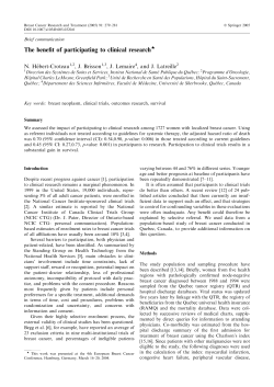
We can also use Excel to derive sample sizes – using the same functionality but in a spreadsheet, this is probably
more aesthetic than the use of a SAS macro, especially for the general population who have an aversion to code!
Example of a spreadsheet output is as follows:
Here using ActiveX controls and Visual Basic, we can set data types and limits for power and significance to provide a
sample size.
OTHER CONSIDERATIONS
There are many other types of trials that need to be considered, such as non-inferiority trials and bioequivalence
trials; we can also base sample size equations on survival data.
We also need to consider that for Phase I trials, quite often there is not enough prior information to provide for these
formula-driven methods. In these cases, a somewhat more pragmatic approach needs to be made towards sample
size – for instance, the FDA guideline (6) states that “a pilot study that documents BE [bioequivalence] can be
appropriate, provided its design and execution are suitable and that a sufficient number of subjects (e.g., 12) have
completed the study.”
Another point to consider is the use of interim analyses – it may be ethically necessary (especially with early phase
trials) for a review of data during the trial to ensure that subject safety is not compromised. To this end, various
stopping rules can be put in place to ensure that (a) the final outcome of the trial is powered effectively and (b) the
ethical constraints are in no way compromised. These methods of “alpha spending” are varied, but some of the more
common methods are detailed in the References (3,4,5).
Another available technique is “bootstrapping” – a simulation method; this is relatively user-intensive but it has the
potential to provide a better sample size estimation than the techniques detailed above (7).
9
PhUSE 2006
CONCLUSION
In general, this paper has concentrated on but a small section of sample size derivation. The examples given merely
scratch the surface of the available methods of determining a sample size. What we need to focus on is that the
study design is the key to an appropriate and robust sample size; this in turn is driven by the trial objectives and
endpoints. By ensuring that reasonable assumptions are made, we can meet ethical and regulatory conformance as
well as providing a firm sample size.
REFERENCES
1.
2.
3.
4.
5.
6.
7.
S. A. Julious (2005); Estimating Sample Sizes in Clinical Research
ICH Topic E9: Statistical Principles for Clinical Trials (1998) http://www.emea.eu.int/pdfs/human/ich/036396en.pdf
P. Armitage, G. Berry, J.N.S Matthews (2002); Statistical Methods in Clinical Research (Fourth Edition)
S. J. Pocock (1998); Clinical Trials – A Practical Approach
S. Senn (1993); Cross-over Trials in Clinical Research
Guideline for Industry – Bioavailability and Bioequivalence Studies for Orally Administered Drug Products (2003)
Efron and Tibshirani (1993); An Introduction to the Bootstrap
ACKNOWLEDGMENTS
Sincerest thanks to Dr Stephen A Julious for allowing me to source some examples from his presentation on
“Estimating Sample Sizes in Clinical Trials”. Also, thanks to Katherine Hutchinson of Oxford Pharmaceutical
Sciences Ltd. for her guidance and patience.
CONTACT INFORMATION
Your comments and questions are valued and encouraged. Contact the author at:
John Salter
Oxford Pharmaceutical Sciences Ltd.
Lancaster House
Kingston Business Park
Kingston Bagpuize
OXFORDSHIRE
OX13 5FE
Work Phone: 01865 823823
Email: [email protected]
Web: www.ops-web.com
SAS and all other SAS Institute Inc. product or service names are registered trademarks or trademarks of SAS
Institute Inc. in the USA and other countries. ® indicates USA registration.
Other brand and product names are trademarks of their respective companies.
10