
Asymptotics for High Dimension, Low Sample Size data
Asymptotics for High Dimension, Low Sample Size data
and Analysis of Data on Manifolds
Sungkyu Jung
A dissertation submitted to the faculty of the University of North Carolina at Chapel
Hill in partial fulfillment of the requirements for the degree of Doctor of Philosophy in
the Department of Statistics and Operations Research (Statistics).
Chapel Hill
2011
Approved by:
Advisor: : Dr. J. S. Marron
Reader: : Dr. Mark Foskey
Reader: : Dr. Jason Fine
Reader: : Dr. Yufeng Liu
Reader: : Dr. Jan Hannig
c 2011
⃝
Sungkyu Jung
ALL RIGHTS RESERVED
ii
ABSTRACT
SUNGKYU JUNG: Asymptotics for High Dimension, Low Sample Size data
and Analysis of Data on Manifolds.
(Under the direction of Dr. J. S. Marron.)
The dissertation consists of two research topics regarding modern non-standard data analytic situations. In particular, data under the High Dimension, Low Sample Size (HDLSS)
situation and data lying on manifolds are analyzed. These situations are related to the statistical image and shape analysis.
The first topic is an asymptotic study of the high dimensional covariance matrix. In particular, the behavior of eigenvalues and eigenvectors of the covariance matrix is analyzed, which
is closely related to the method of Principal Component Analysis (PCA). The asymptotic
behavior of the Principal Component (PC) directions, when the dimension tends to infinity
with the sample size fixed, is investigated. We have found mathematical conditions which
characterize the consistency and the strong inconsistency of the empirical PC direction vectors. Moreover, the conditions where the empirical PC direction vectors are neither consistent
nor strongly inconsistent are revealed, and the limiting distributions of the angle formed by
the empirical PC direction and the population counterpart are presented. These findings help
to understand the use of PCA in the HDLSS context, which is justified when the conditions
for the consistency occur.
The second part of the dissertation studies data analysis methods for data lying in curved
manifolds that are the features from shapes or images. A common goal in statistical shape
analysis is to understand variation of shapes. As a means of dimension reduction and visualization, there is a need to develop PCA-like methods for manifold data. We propose flexible
extensions of PCA to manifold data: Principal Arc Analysis and Analysis of Principal Nested
Spheres. The methods are implemented to two important types of manifolds. The sample
space of the medial representation of shapes, frequently used in image analysis to parameterize the shape of human organs, naturally forms curved manifolds, which we characterize
as direct product manifolds. Another type of manifolds we consider is the landmark-based
iii
shape space, proposed by Kendall. The proposed methods in the dissertation capture major
variations along non-geodesic paths. The benefits of the methods are illustrated by several
data examples from image and shape analysis.
iv
ACKNOWLEDGEMENTS
I thank Professor Steve Marron for his advice and support. His support enabled me to enjoy my
research and to complete the dissertation work successfully. He helped me explore the subject
with his keen insight, and provided many opportunities for various kinds of collaborative
research. Every result in the dissertation is indepted to his guidance.
This dissertation work would have not been completed without valuable comments and
suggestions of coauthors. Professor Arush Sen lead me to take another leap in the theoretical
part of the dissertation in Chapter 3. Dr. Mark Foskey proposed to use small circles, and
investigations since then results in the work presented in Chapter 6. Professor Ian Dryden
introduced statistical shape analysis in which Chapter 7 is rooted. Professor Steve Pizer introduced the broad area of image analysis and motivated to develop Part II of the dissertation.
I wish to express my sincere appreciation to senior researchers for their valuable advice.
Professor Steve Pizer has been a great mentor. Conversations with him on topics ranging from
personal life decisions to deep mathematical questions have helped me a lot during the Ph.D.
program. Professor Jason Fine and Professor Yufeng Liu gave me advices in making difficult
decisions. I also appreciate valuable academic discussions and conversations with Professor
Stephan Huckemann, Professor Anuj Srivastava, Professor Hongtu Zhu, Dr. Xiaoxiao Liu,
Dr. Ja-Yeon Jeong and the community of MIDAG.
My life at Chapel Hill during the program was happy and fulfilling. I can not imagin it
without friends: Classmates, gangs who flocked at Baity Hill and Finley Forest, and basketball
and tennis players I loved to play with. I must thank my family—parents, my sister and her
family—who have been very supportive in planning and achieving my life goal.
Last, my deepest gratitude goes to my wife, Seo Young, for her kindness as family and for
valuable opinions as a fellow statistician. She always believes in me and helps to reach greater
goals. For your patience and understanding, I will always love you, Seo Young.
v
Contents
ACKNOWLEDGEMENTS
v
List of Figures
x
List of Tables
xii
1 Introduction
I
1
1.1
Motivations and Problems . . . . . . . . . . . . . . . . . . . . . . . . . . . . . .
1
1.2
Summary and Contributions . . . . . . . . . . . . . . . . . . . . . . . . . . . . .
4
PCA in High Dimension, Low Sample Size Context
2 PCA consistency in HDLSS context
2.1
9
Introduction and summary . . . . . . . . . . . . . . . . . . . . . . . . . . . . .
2.1.1
8
9
General setting . . . . . . . . . . . . . . . . . . . . . . . . . . . . . . . . 12
2.2
HDLSS asymptotic behavior of the sample covariance matrix . . . . . . . . . . 14
2.3
Geometric representation of HDLSS data . . . . . . . . . . . . . . . . . . . . . 17
2.4
Consistency and strong inconsistency of PC directions . . . . . . . . . . . . . . 19
2.5
2.4.1
Criteria for consistency or strong inconsistency of the first PC direction
20
2.4.2
Generalizations . . . . . . . . . . . . . . . . . . . . . . . . . . . . . . . . 21
2.4.3
Main theorem . . . . . . . . . . . . . . . . . . . . . . . . . . . . . . . . . 23
2.4.4
Corollaries to the main theorem
2.4.5
Limiting distributions of corresponding eigenvalues . . . . . . . . . . . . 26
. . . . . . . . . . . . . . . . . . . . . . 25
Proofs . . . . . . . . . . . . . . . . . . . . . . . . . . . . . . . . . . . . . . . . . 27
vi
3 Boundary Behavior in HDLSS asymptotics of PCA
3.1
Introduction . . . . . . . . . . . . . . . . . . . . . . . . . . . . . . . . . . . . . . 41
3.2
Range of limits in the single spike model . . . . . . . . . . . . . . . . . . . . . . 43
3.3
Limits under generalized spiked covariance model . . . . . . . . . . . . . . . . . 45
3.3.1
Eigenvalues and eigenvectors . . . . . . . . . . . . . . . . . . . . . . . . 46
3.3.2
Angles between principal component spaces . . . . . . . . . . . . . . . . 51
3.4
Geometric representations of the HDLSS data . . . . . . . . . . . . . . . . . . . 56
3.5
Derivation of the density functions . . . . . . . . . . . . . . . . . . . . . . . . . 60
4 Discussions on High Dimensional Asymptotic Studies
II
41
64
4.1
Different regimes in high-dimensional asymptotics
. . . . . . . . . . . . . . . . 64
4.2
Open problems . . . . . . . . . . . . . . . . . . . . . . . . . . . . . . . . . . . . 66
Statistics on Manifold
68
5 Data on manifolds
69
5.1
Manifolds of interest . . . . . . . . . . . . . . . . . . . . . . . . . . . . . . . . . 69
5.2
Mathematical background . . . . . . . . . . . . . . . . . . . . . . . . . . . . . . 72
5.3
5.4
5.2.1
Riemannian manifold . . . . . . . . . . . . . . . . . . . . . . . . . . . . 72
5.2.2
Direct Product manifold . . . . . . . . . . . . . . . . . . . . . . . . . . . 75
Exploratory Statistics on manifolds . . . . . . . . . . . . . . . . . . . . . . . . . 78
5.3.1
Extrinsic and Intrinsic means . . . . . . . . . . . . . . . . . . . . . . . . 78
5.3.2
Examples: Geodesic Means on Various Manifolds . . . . . . . . . . . . . 80
Backward Generalization of PCA on manifolds . . . . . . . . . . . . . . . . . . 87
6 Principal Arc Analysis on direct product manifold
91
6.1
Introduction . . . . . . . . . . . . . . . . . . . . . . . . . . . . . . . . . . . . . . 91
6.2
Circle class for non-geodesic variation on S 2 . . . . . . . . . . . . . . . . . . . . 94
6.3
Suppressing small least-squares circles . . . . . . . . . . . . . . . . . . . . . . . 99
6.4
Principal Arc Analysis on direct product manifolds . . . . . . . . . . . . . . . . 106
6.4.1
Choice of the transformation hδ¯ . . . . . . . . . . . . . . . . . . . . . . . 109
vii
6.5
6.6
Application to m-rep data . . . . . . . . . . . . . . . . . . . . . . . . . . . . . . 111
6.5.1
The Medial Representation of prostate . . . . . . . . . . . . . . . . . . . 111
6.5.2
Simulated m-rep object . . . . . . . . . . . . . . . . . . . . . . . . . . . 112
6.5.3
Prostate m-reps from real patients . . . . . . . . . . . . . . . . . . . . . 113
Doubly iterative algorithm to find the least-squares small circle . . . . . . . . . 114
7 Analysis of Principal Nested Spheres
119
7.1
Introduction . . . . . . . . . . . . . . . . . . . . . . . . . . . . . . . . . . . . . . 119
7.2
Principal Nested Spheres . . . . . . . . . . . . . . . . . . . . . . . . . . . . . . . 122
7.2.1
Geometry of Nested Spheres . . . . . . . . . . . . . . . . . . . . . . . . . 122
7.2.2
The Best Fitting Subsphere . . . . . . . . . . . . . . . . . . . . . . . . . 124
7.2.3
The sequence of Principal Nested Spheres . . . . . . . . . . . . . . . . . 124
7.2.4
Euclidean-type representation . . . . . . . . . . . . . . . . . . . . . . . . 125
7.2.5
Principal Arcs . . . . . . . . . . . . . . . . . . . . . . . . . . . . . . . . 126
7.2.6
Principal Nested Spheres restricted to Great Spheres . . . . . . . . . . . 127
7.3
Visualization of nested spheres of S 3 . . . . . . . . . . . . . . . . . . . . . . . . 128
7.4
Prevention of overfitting by sequential tests . . . . . . . . . . . . . . . . . . . . 130
7.4.1
Likelihood ratio test . . . . . . . . . . . . . . . . . . . . . . . . . . . . . 130
7.4.2
Parametric bootstrap test . . . . . . . . . . . . . . . . . . . . . . . . . . 131
7.4.3
Application procedure . . . . . . . . . . . . . . . . . . . . . . . . . . . . 132
7.5
Computational Algorithm . . . . . . . . . . . . . . . . . . . . . . . . . . . . . . 134
7.6
Application to Shape space . . . . . . . . . . . . . . . . . . . . . . . . . . . . . 136
7.6.1
Planar shape space . . . . . . . . . . . . . . . . . . . . . . . . . . . . . . 136
7.6.2
Principal Nested Spheres for planar shapes . . . . . . . . . . . . . . . . 137
7.6.3
Principal Nested Spheres for spaces of m > 2 dimensional shapes . . . . 140
7.7
Real Data Analysis . . . . . . . . . . . . . . . . . . . . . . . . . . . . . . . . . . 141
7.8
Geometry of Nested Spheres . . . . . . . . . . . . . . . . . . . . . . . . . . . . . 148
7.8.1
Preliminary Transformations: Rotation matrices . . . . . . . . . . . . . 148
7.8.2
Geometry of Subsphere . . . . . . . . . . . . . . . . . . . . . . . . . . . 149
7.8.3
Geometry of Nested Spheres . . . . . . . . . . . . . . . . . . . . . . . . . 152
viii
7.9
Proofs and Additional Lemmas . . . . . . . . . . . . . . . . . . . . . . . . . . . 154
Bibliography
160
ix
List of Figures
2.1
Example showing that PCA works in the HDLSS context . . . . . . . . . . . . 10
2.2
Examples of the ϵ-conditions . . . . . . . . . . . . . . . . . . . . . . . . . . . . 17
2.3
Cartoon illustrates the consistency in HDLSS context . . . . . . . . . . . . . . 20
3.1
Density functions of the limiting distributions of the angle between u1 and u
ˆ1 . 45
3.2
The limiting distribution of the angles for the m = 2 case . . . . . . . . . . . . 55
3.3
Limiting distributions of the Euclidean sine distance . . . . . . . . . . . . . . . 56
3.4
The three different HDLSS geometric representations . . . . . . . . . . . . . . . 59
5.1
Extrinsic Mean and Intrinsic Mean on the circle . . . . . . . . . . . . . . . . . . 79
5.2
Geodesic mean set on S 1 . . . . . . . . . . . . . . . . . . . . . . . . . . . . . . . 82
5.3
Geodesic mean set on S 2 . . . . . . . . . . . . . . . . . . . . . . . . . . . . . . . 83
5.4
Geodesic mean set on S 1 × S 1 . . . . . . . . . . . . . . . . . . . . . . . . . . . . 85
5.5
Example of a geodesic mean on S 2 . . . . . . . . . . . . . . . . . . . . . . . . . 85
5.6
Forward and Backward viewpoints of PCA
6.1
S 2 -valued samples of the prostate m-reps . . . . . . . . . . . . . . . . . . . . . 93
6.2
Four generic distributions on a sphere . . . . . . . . . . . . . . . . . . . . . . . 97
6.3
Illustration of the signal+error model for a circle in S 2 . . . . . . . . . . . . . . 101
6.4
Overlaid target densities in suppressing small circles . . . . . . . . . . . . . . . 102
6.5
Simulation results for the estimation of the signal-to-noise ratio . . . . . . . . . 105
6.6
Illustration of the discontinuity between small and great circles . . . . . . . . . 107
6.7
The transformation hδ : S 2 → R2 . . . . . . . . . . . . . . . . . . . . . . . . . . 111
6.8
The prostate m-rep, revisited. . . . . . . . . . . . . . . . . . . . . . . . . . . . . 112
6.9
Scree plots and Scatter plots to compare PGA and PAA.
. . . . . . . . . . . . . . . . . . . . 88
. . . . . . . . . . . . 114
6.10 The first principal component arcs (geodesics) with data. . . . . . . . . . . . . 115
6.11 Scatter plots of PGA and PAA from real patients data. . . . . . . . . . . . . . 115
7.1
Human movement data shows more effective non-geodesic decomposition. . . . 121
x
7.2
Idea of PNS, illustrated. . . . . . . . . . . . . . . . . . . . . . . . . . . . . . . . 123
7.3
Visualization of nested spheres. . . . . . . . . . . . . . . . . . . . . . . . . . . . 129
7.4
Two different null hypothesis in prevention of overfitting of PNS. . . . . . . . . 131
7.5
Migration path of an elephant seal. . . . . . . . . . . . . . . . . . . . . . . . . . 142
7.6
Scatterplots for sand grain data. . . . . . . . . . . . . . . . . . . . . . . . . . . 144
7.7
Sand grain configurations with sea and river groups. . . . . . . . . . . . . . . . 144
7.8
Human movement data overlay. . . . . . . . . . . . . . . . . . . . . . . . . . . . 145
7.9
Human movement data with fitted curves. . . . . . . . . . . . . . . . . . . . . . 146
7.10 Rat skull growth data. . . . . . . . . . . . . . . . . . . . . . . . . . . . . . . . . 147
7.11 The first principal mode in rat skull growth data. . . . . . . . . . . . . . . . . . 147
7.12 Hierarchical structure of the sequence of nested spheres of the 3-sphere. . . . . 153
xi
List of Tables
6.1
Simulation results for the estimation of the signal-to-noise ratio . . . . . . . . . 105
xii
Chapter 1
Introduction
This dissertation demonstrates development, theoretical study, and implementation of statistical methods for non-standard data, where conventional statistical methods are sometimes
not directly applicable. The non-standard data are increasingly emerging, examples of which
are the data with High Dimension, Low Sample Size (HDLSS, or the large p, small n) and
the data that naturally lie on curved manifolds. Specifically, datasets with those properties
are frequently observed in image and shape analysis, genomics, and functional data. These
application areas together span a new statistical field in which traditional concepts need to be
re-considered and development of new methodologies is required. The dissertation addresses
two important aspects of this broad field: The HDLSS asymptotics, where the limiting operation has the dimension growing with the sample size fixed, to understand the use of Principal
Component Analysis (PCA) in the HDLSS context; Development of PCA-like methods for
manifold data, where the proposed methods intuitively capture major non-linear variations in
lower dimension.
1.1
Motivations and Problems
The work is mainly motivated by statistical problems arising in image and shape analysis. The
image analysis concerns extraction of information from an image, or set of images, usually in a
digital form. The field of image analysis is broad, where mathematician, computer scientists,
engineers, medical researchers and statisticians have contributed in different aspects of the
area, separately or in collaborative fashion. Statistical image analysis puts a distributional
assumption on images (either on the population of images or an image itself), develops sta-
tistical procedures to obtain meaningful information from the images. A subcategory of the
broad field concerns an object found in images (e.g. human brain from an image of MRI),
where the set of objects is under investigation. The statistical shape analysis focuses on the
object shape in the image.
A shape can be represented by many different methods, examples of which are the medial representations (Siddiqi and Pizer (2008)), a point correspondence model and spherical
harmonic representations (Gerig et al. (2004)), the traditional landmark-based shapes (Bookstein (1991), Dryden and Mardia (1998)) and a newly developed functional representation
for shapes (Srivastava et al. (2010)). A challenge in shape analysis is that natural sample
spaces of those shape representations are usually not Euclidean spaces but curved manifolds.
In particular, the statistical methods that benefit from Euclidean geometry are not directly
applicable for the manifold-valued objects. This motivates statistical study of manifold-valued
random variables.
Another challenge in the image analysis is that the dimensionality of the representations
is very high. Due to advances in modern technology, obtaining high resolution images became
easier. However, the sample size (i.e. the number of observations) stays low especially in the
medical image analysis because of the high cost in obtaining medical images such as MRI and
CT. Hall et al. (2005) termed the situation as High Dimension, Low Sample Size (HDLSS)
context, which becomes increasingly common and is observed not only in medical imaging but
also in genomics, chemometrics, and functional analysis.
In the broad field of image analysis, we focus on data analyses in the sample space of the
representations, called feature space. Specifically, we wish to give insight into the following
basic statistical tasks:
1. Exploratory statistics and visualization of important structure: Given a random object
or a set of observations of those in a non-Euclidean and multi-dimensional feature space,
the first task for a statistician is to provide exploratory statistics. This includes finding
a central location (mean), measure of variability (variance), and patterns in the data
set.
2. Dimension reduction: When the dimension of the Euclidean feature space is high, we
2
wish to find an affine subspace of smaller dimension in a way that we do not lose
important variation. If the feature space is a non-Euclidean curved manifold, we wish
to find a sub-manifold of smaller dimension with great variance contained.
3. Estimation of probability distribution: A probability distribution can be assumed with
fewer parameters if we choose to work with the subspace (or the sub-manifold) found in
the dimension reduction.
The Principal Component Analysis (PCA) plays an important role in all of those problems.
PCA is often used in multivariate analysis for dimension reduction and visualization of
important modes of variation. It is also understood as an estimation of the population principal components by the sample principal components. PCA is commonly credited to Hotelling
(1933) and its common references are Muirhead (1982) and Jolliffe (2002). The objective of
PCA is to capture most of the variability, of a multidimensional random vector or a set of
observations consisting of a large number of measurements, in a low dimensional subspace.
When the sample space is a Euclidean (linear) space, PCA finds a sequence of affine subspaces
or a set of orthogonal direction vectors. Optimal choice of this sequence can be characterized
in two equivalent ways: maximization of the variance captured by the affine subspace or minimization of the variance of the residuals. In the Euclidean space, PCA is usually computed
through the eigen-decomposition of covariance matrices.
We discuss two different views of the PCA, namely the forward and backward stepwise
views, later in Part II of the dissertation. These views are first introduced in Marron et al.
(2010), which stems from the work in this dissertation.
Now, consider using PCA in the image or shape analysis, which in fact is a common routine
for data analysts. While the traditional PCA is well defined for random vectors, we have two
concerns; First of all, the sample size is usually too low but the dimension of the sample space
is very high; Second, the natural sample space of the features of images or shapes is not the
flat Euclidean space, but a curved manifold. A simple application of Euclidean PCA usually
fails in the case. There are two different but related research questions:
1. What is the behavior of PCA in the high dimension low sample size context?
2. How to generalize PCA for manifold-valued objects?
3
Part I and II of the dissertation answer the first and second questions, respectively. A
short summary is given in the next section.
1.2
Summary and Contributions
In Part I of the dissertation, Euclidean PCA is asymptotically studied when the dimension d
grows, while the sample size n is fixed. In particular, we are interested in the situations when
the PCA works in the HDLSS situation and when it fails. The success and failure of PCA are
well described by the consistency of the empirical Principal Component (PC) directions u
ˆi (or
the ith eigenvector of the covariance matrix, see Section 2.1) with its population counterpart
ui , under the limiting operation d → ∞ and n fixed. Since the size of the direction vectors
ui , u
ˆi are increasing as d grows, the discrepancy between directions is measured by the angle
formed by the directions. We say u
ˆi is :
• consistent with ui if Angle(ˆ
ui , ui ) → 0 as d → ∞;
• strongly inconsistent with ui if Angle(ˆ
ui , ui ) → π/2 as d → ∞.
While the consistency is the case we desire, the strong inconsistency is somewhat counterintuitive since the angle π/2 is indeed the largest possible value of the angle. In other words,
the estimate u
ˆi of ui loses its connection to the population structure and becomes completely
arbitrary. We see that in HDLSS asymptotics when u
ˆi is not consistent, it is often not just
inconsistent but strongly inconsistent. The mathematical mechanism of these situations is the
main topic of Chapter 2. In short, when the population PC variance is large such as of order
dα , α > 1, the corresponding PC direction estimate is consistent. If not so large, i.e. α < 1,
then the corresponding PC direction estimate is strongly inconsistent.
The distributional assumptions in the study are general and intuitive. Gaussianity is
relaxed into a ρ-mixing under some permutation and a moment condition. While the ρmixing assumption is most appropriate for a time series data set (because of the ordering
of the variables), we relax the assumption by allowing any permutation of variable ordering.
Thus the assumption makes sense for gene expression microarray data and image or shape
data. See Section 2.1.1 for detailed assumptions.
4
We also considered a case where PC directions are not distinguishable, which occurs when
some eigenvalues of the covariance matrix are identical. In Chapter 2, we consider a subspace spanned by those indistinguishable PC directions, and develop a notion of subspace
consistency.
A natural question arises after we see that the exponent α in the order of PC variance
dα is the main driver between consistency (α > 1) and strong inconsistency (α < 1). What
can we expect at the boundary between two cases? Chapter 3 discusses topics related to this
question. We find that the angles do not degenerate (either to 0 or π/2) but weakly converge to
distributions with support in (0, π/2). We provide explicit forms of the limiting distributions
in Sections 3.2 and 3.3. We further extend the HDLSS geometric representation (i.e. modulo
rotation, n independent samples converge to vertices of a regular n simplex) found in Hall
et al. (2005) and Ahn et al. (2007) into three different HDLSS representations, which gives an
intuition in understanding a transition between consistency and strong inconsistency.
Part I of the dissertation is concluded with a discussion on open problems and a literature
review; see Chapter 4.
The second part of the dissertation introduces some developments in generalization of
PCA to manifold-valued data. We begin by introducing examples of specific manifolds, that
are feature spaces in image analysis (Section 5.1). This gives a motivation to focus on specific
types of manifolds. We briefly describe some basic Riemannian geometry used in the analysis
and some specific manifolds we focus in Section 5.2. In particular, we focus on spheres and
direct product of those with Euclidean space.
A common goal in analyzing these manifold data is to understand the variability. PCA,
when appropriately modified and implemented for manifolds, provides a very effective means
of analyzing the major modes of variation. The main contribution of Part II is to provide
flexible extensions of PCA to manifold data. Briefly, the main idea in improving PCA is to
make the method adaptive to certain non-linear structures of the data while the desirable
properties of PCA are inherited.
To elaborate the work intuitively, let us assume that the manifold is the usual unit sphere
S 2 := {x ∈ R3 : ∥x∥ = 1}. An analogue of a straight line on a sphere is a great circle, also
referred to as a geodesic. A principal component direction on the sphere is represented by
5
a great circle. As in the standard PCA, one may find a mean first then fit a great circle as
the first PC direction. The second and higher PC directions are found among all great circles
orthogonal to the first PC (geodesic). However, we found out that this standard approach may
lead to an ineffective representation of the data, as discussed in Section 6.2. To resolve this
issue, we took a reverse viewpoint in generalizing PCA, called backward approach, where the
dimensionality of approximating subspaces (or submanifolds) is successively reduced. That
is, analogous to the backward variable selection in regression, we remove the least important
component first. This backward approach agrees with the standard PCA in Euclidean space
but not in manifolds. The backward stepwise viewpoint gives a common root in generalization
of PCA to non-linear spaces. In Section 5.4 the two different viewpoints of the usual PCA is
discussed, and we point out that the backward approach is suitable for extension of PCA to
manifold data.
The backward approach not only works well when the standard approach fails, but also
gives a flexibility in capturing variations. The generalized PCA by the backward approach
can be relaxed to find a small circle (e.g. the Tropic of Cancer) of the sphere, adaptive to the
data. The resulting principal arcs capture the variation in the data set more succinctly and
serve as principal components for visualization and dimension reduction.
The two methods proposed in Part II are generalizations of PCA to manifold-valued variables. Chapter 6 discusses Principal Arc Analysis for direct product manifolds; Chapter
7 discusses Analysis of Principal Nested Spheres for hyperspheres and the shape spaces of
Kendall (1984).
The direct product manifold is a class of specially structured manifolds. The sample
spaces of medial shape representations, diffeomorphisms, point distribution models, points
and normals models and size-and-shapes can all be considered as a special form of direct
product manifolds. We propose to use a transformation of non-Euclidean data into Euclidean
coordinates, then a composite space of Euclidean data and the transformed non-Euclidean
data gives a space suitable for further analysis including non-linear dimension reduction,
visualization, and modeling with fewer parameters. Principal Arc Analysis consists of 1)
estimation of the principal circle, which is the basis for transformations, 2) choices of the
transformations, and 3) ad-hoc tests to suppress overfitting in principal arcs. Chapter 6 also
6
discusses an application of Principal Arc Analysis to medial shape representations data set.
Analysis of Principal Nested Spheres can be viewed as an extension of Principal Arc
Analysis to higher dimensional spheres S d and Kendall’s shape space. Since the dimension of
the sphere is now higher than the simple 2, the geometry involved is a bit more complicated
than the usual sphere. We define nested spheres, which are in a special form of sub-manifolds of
S d , as a basis for decomposition of the hypersphere. Geometry of nested spheres are discussed
in depth in Section 7.8. Simply put, Principal Nested Spheres are fitted nested spheres that
capture most of the variances in the data. We discuss application of Analysis of Principal
Nested Spheres to Kendall’s shape space in Section 7.6, as well as several real data examples
in Section 7.7. We exemplify that the proposed method results in a succinct description of
real data set in fewer dimension than alternative methods in literature.
7
Part I
PCA in High Dimension, Low
Sample Size Context
8
Chapter 2
PCA consistency in HDLSS context
Since traditional tools of multivariate statistical analysis were designed for the n > d case, it
should not be surprising that they often do not work properly for the HDLSS data. However,
the method of PCA has been seen to sometimes be very effective in the HDLSS context, and is
widely used as a dimension reduction technique. In this chapter we investigate the asymptotic
behaviors of PCA when d tends to infinity while n is fixed, which provide the appropriate
analysis to study the HDLSS context. In short, the asymptotics characterizes when Euclidean
PCA works and when it fails. The work presented in this chapter is based on Jung and Marron
(2009).
2.1
Introduction and summary
The High Dimension, Low Sample Size (HDLSS) data situation occurs in many areas of
modern science and the asymptotic studies of this type of data are becoming increasingly
relevant. We will focus on the case that the dimension d increases while the sample size n is
fixed as done in Hall et al. (2005) and Ahn et al. (2007). The d-dimensional covariance matrix
is challenging to analyze in general since the number of parameters is
d(d+1)
,
2
which increases
even faster than d. Instead of assessing all of the parameter estimates, the covariance matrix
is usually analyzed by Principal Component Analysis (PCA). PCA is often used to visualize
important structure in the data, as shown in Figure 2.1. The data in Figure 1, described in
detail in Bhattacharjee et al. (2001) and Liu et al. (2008), are from a microarray study of lung
cancer. Different symbols correspond to cancer subtypes and Figure 2.1 shows the projections
of the data onto the subspaces generated by PC1 and PC2 (left panel) and PC1 and PC3
40
20
20
PC 1
PC 1
40
0
−20
0
−20
−20
0
20
40
−40
PC 2
−20
0
20
PC 3
Figure 2.1: Scatterplots of data projected on the first three PC directions. The dataset contains 56
patients with 2530 genes. There are 20 Pulmonary Carcinoid (plotted as +), 13 Colon
Cancer Metastases (∗), 17 Normal Lung (◦), and 6 Small Cell Carcinoma (×). In spite of
the high dimensionality, PCA reveals important structure in the data.
(right panel, respectively) directions. This shows the difference between subtypes is so strong
that it drives the first three principal components. This illustrates common occurrence: the
data have important underlying structure which is revealed by the first few PC directions.
PCA is also used to reduce dimensionality by approximating the data with the first few
principal components.
For both visualization and data reduction, it is critical that the PCA empirical eigenvectors reflect true underlying distributional structure. Hence our focus is on the underlying
mechanism which determines when the sample PC directions converge to their population
counterparts as d → ∞. For example, we quantify situations where the dominant sample
eigenvectors are revealing important underlying structure in the data as in Figure 2.1. In general we assume d > n. Since the size of the covariance matrix depends on d, the population
covariance matrix is denoted as Σd and similarly the sample covariance matrix, Sd , so that
their dependency on the dimension is emphasized. PCA is done by eigen-decomposition of a
covariance matrix. The eigen-decomposition of Σd is
Σd = Ud Λd Ud′ ,
10
where Λd is a diagonal matrix of eigenvalues λ1,d > λ2,d > · · · > λd,d and Ud is a matrix of
corresponding eigenvectors so that Ud = [u1,d , u2,d , . . . , ud,d ]. Sd is similarly decomposed as
ˆd Λ
ˆ dU
ˆ′.
Sd = U
d
Ahn et al. (2007) developed the concept of HDLSS consistency which was the first investigation of when PCA could be expected to find important structure in HDLSS data. Our
main results are formulated in terms of three related concepts:
1. consistency: The direction u
ˆi,d is consistent with its population counterpart ui,d if
Angle(ui,d , u
ˆi,d ) −→ 0 as d → ∞. The growth of dimension can be understood as
adding more variation. The consistency of sample eigenvectors occurs when the added
variation supports the existing structure in the covariance or is small enough to be
ignored.
2. strong inconsistency: In situations where u
ˆi,d is not consistent, a perhaps counterintuitive HDLSS phenomenon frequently occurs. In particular, u
ˆi,d is said to be strongly
inconsistent with its population counterpart ui,d in the sense that it tends to be as
far away from ui,d as possible, that is, Angle(ui,d , u
ˆi,d ) −→
π
2
as d → ∞. Strong in-
consistency occurs when the added variation obscures the underlying structure of the
population covariance matrix.
3. subspace consistency: When several population eigenvalues indexed by j ∈ J are similar,
the corresponding sample eigenvectors may not be distinguishable. In this case, u
ˆj,d will
not be consistent for uj,d but will tend to lie in the linear span, span{uj,d : j ∈ J}. This
motivates the definition of convergence of a direction u
ˆi,d to a subspace, called subspace
consistency;
Angle(ˆ
ui,d , span{uj,d : j ∈ J}) −→ 0
as d → ∞. This definition essentially comes from the theory of canonical angles discussed by Gaydos (2008). That theory also gives a notion of convergence of subspaces,
that could be developed here.
In this chapter, a broad and general set of conditions for consistency and strong inconsis-
11
tency are provided. Section 2.2 develops conditions that guarantee the non-zero eigenvalues
of the sample covariance matrix tend to a increasing constant, which are much more general
than those of Hall et al. (2005) and Ahn et al. (2007). This asymptotic behavior of the sample
covariance matrix is the basis of the geometric representation of HDLSS data. Our result
gives broad new insight into this representation as discussed in section 2.3. The central issue
of consistency and strong inconsistency is developed in section 2.4, as a series of theorems.
For a fixed number κ, we assume the first κ eigenvalues are much larger than the others. We
show that when κ = 1, the first sample eigenvector is consistent and the others are strongly
inconsistent. We also generalize to the κ > 1 case, featuring two different types of results
(consistency and subspace consistency) according to the asymptotic behaviors of the first κ
eigenvalues. All results are combined and generalized in the main theorem (Theorem 2.5).
Proofs of theorems are given in section 2.5.
Further discussions on the boundary case where the PC directions are neither consistent
nor strongly inconsistent are deferred to Chapter 3. Relevant literatures are reviewed and
discussed later at Chapter 4.
2.1.1
General setting
Suppose we have a d × n data matrix X(d) = [X1,(d) , . . . , Xn,(d) ] with d > n, where the
d-dimensional random vectors X1,(d) , . . . , Xn,(d) are independent and identically distributed.
We assume that each Xi,(d) follows a multivariate distribution (which does not have to be
Gaussian) with mean zero and covariance matrix Σd . Define the sphered data matrix Z(d) =
−1/2
Λd
Ud′ X(d) . Then the components of the d × n matrix Z(d) have unit variances, and are
uncorrelated with each other. We shall regulate the dependency (recall for non-Gaussian data,
uncorrelated variables can still be dependent) of the random variables in Z(d) by a ρ-mixing
condition. This allows serious weakening of the assumptions of Gaussianity while still enabling
the law of large numbers that lie behind the geometric representation results of Hall et al.
(2005).
The concept of ρ-mixing was first developed by Kolmogorov and Rozanov (1960). See
Bradley (2005) for a clear and insightful discussion. For −∞ 6 J 6 L 6 ∞, let FJL denote
the σ-field of events generated by the random variables (Zi , J 6 i 6 L). For any σ-field A, let
12
L2 (A) denote the space of square-integrable, A measurable (real-valued) random variables.
For each m > 1, define the maximal correlation coefficient
j
∞
f ∈ L2 (F−∞
), g ∈ L2 (Fj+m
),
ρ(m) := sup |corr(f, g)|,
where sup is over all f , g and j ∈ Z. The sequence {Zi } is said to be ρ-mixing if ρ(m) → 0
as m → ∞.
While the concept of ρ-mixing is useful as a mild condition for the development of laws of
large numbers, its formulation is critically dependent on the ordering of variables. For many
interesting data types, such as microarray data, there is clear dependence but no natural
ordering of the variables. Hence we assume that there is some permutation of the data which
is ρ-mixing. In particular, let {Zij,(d) }di=1 be the components of the jth column vector of Z(d) .
We assume that for each d, there exists a permutation πd : {1, . . . , d} 7−→ {1, . . . , d} so that
the sequence {Zπd (i)j,(d) : i = 1, . . . , d} is ρ-mixing.
In the following, all the quantities depend on d, but the subscript d will be omitted for
the sake of simplicity when it does not cause any confusion. The sample covariance matrix is
defined as S = n−1 XX ′ . We do not subtract the sample mean vector because the population
mean is assumed to be 0. Since the dimension of the sample covariance matrix S grows, it
is challenging to deal with S directly. A useful approach is to work with the dual of S. The
dual approach switches the role of columns and rows of the data matrix, by replacing X by
X ′ . The n × n dual sample covariance matrix is defined as SD = n−1 X ′ X. An advantage of
1
this dual approach is that SD and S share non-zero eigenvalues. If we write X as U Λ 2 Z and
use the fact that U is a unitary matrix,
′
1
2
′
′
1
2
nSD = (Z Λ U )(U Λ Z) = Z ΛZ =
d
∑
λi,d zi′ zi ,
(2.1)
i=1
where the zi ’s, i = 1, . . . , d, are the row vectors of the matrix Z. Note that nSD is commonly
referred to as the Gram matrix, consisting of inner products between observations.
13
2.2
HDLSS asymptotic behavior of the sample covariance matrix
In this section, we investigate the behavior of the sample covariance matrix S when d → ∞
and n is fixed. Under mild and broad conditions, the eigenvalues of S, or the dual SD , behave
asymptotically as if they are from the identity matrix. That is, the set of sample eigenvectors
tends to be an arbitrary choice. This lies at the heart of the geometric representation results
of Hall et al. (2005) and Ahn et al. (2007) which are studied more deeply in section 2.3. We
will see that this condition readily implies the strong inconsistency of sample eigenvectors, see
Theorem 2.5.
The conditions for the theorem are conveniently formulated in terms of a measure of
sphericity
∑
( di=1 λi,d )2
tr2 (Σ)
= ∑d
,
ϵ≡
dtr(Σ2 )
d i=1 λ2i,d
proposed and used by John (1971, 1972) as the basis of a hypothesis test for equality of
eigenvalues. Note that these inequalities always hold:
1
6 ϵ 6 1.
d
Also note that perfect sphericity of the distribution (i.e. equality of eigenvalues) occurs only
when ϵ = 1. The other end of the ϵ range is the most singular case where in the limit as the
first eigenvalue dominates all others.
Ahn et al. (2007) claimed that if ϵ ≫ d1 , in the sense that ϵ−1 = o(d), then the eigenvalues
of SD tend to be identical in probability as d → ∞. However, they needed an additional
assumption (e.g. a Gaussian assumption on X(d) ) to have independence among components
of Z(d) , as described in example 2.1. We extend this result to the case of arbitrary distributions
with dependency regulated by the ρ-mixing condition as in section 2.1.1, which is much more
general than either a Gaussian or an independence assumption. We also explore convergence
in the almost sure sense with stronger assumptions. Our results use a measure of sphericity for
part of the eigenvalues for conditions of a.s. convergence and also for later use in section 2.4.
14
In particular, define the measure of sphericity for {λk,d , . . . , λd,d } as
ϵk ≡
(
∑d
d
i=k
∑d
λi,d )2
i=k
λ2i,d
.
For convenience, we name several assumptions used in this chapter made about the measure
of sphericity ϵ:
• The ϵ-condition: ϵ ≫ d1 , i.e.
∑d
−1
(dϵ)
=
2
i=1 λi,d
∑
( di=1 λi,d )2
→ 0 as d → ∞.
(2.2)
• The ϵk -condition: ϵk ≫ d1 , i.e.
∑d
2
i=k λi,d
(dϵk )−1 = ∑d
→ 0 as d → ∞.
( i=k λi,d )2
• The strong ϵk -condition: For some fixed l > k, ϵl ≫
1
d− 2 ϵ−1
l
√1 ,
d
(2.3)
i.e.
1 ∑
d 2 di=l λ2i,d
= ∑d
→ 0 as d → ∞.
( i=l λi,d )2
(2.4)
Remark 2.1. Note that the ϵk -condition is identical to the ϵ-condition when k = 1. Similarly,
the strong ϵk -condition is also called the strong ϵ-condition when k = 1. The strong ϵk condition is stronger than the ϵk condition if the minimum of l’s which satisfy (2.4), lo , is as
small as k. But, if lo > k, then this is not necessarily true. We will use the strong ϵk -condition
combined with the ϵk -condition.
Note that the ϵ-condition is quite broad in the spectrum of possible values of ϵ: It only
avoids the most singular case. The strong ϵ-condition further restricts ϵl to essentially in the
range ( √1d , 1].
The following theorem states that if the (strong) ϵ-condition holds for Σd , then the sample
eigenvalues behave as if they are from a scaled identity matrix. It uses the notation In for the
n × n identity matrix.
15
Theorem 2.1. For a fixed n, let Σd = Ud Λd Ud′ , d = n+1, n+2, . . . be a sequence of covariance
matrices. Let X(d) be a d × n data matrix from a d-variate distribution with mean zero and
ˆd Λ
ˆ dU
ˆ ′ be the sample covariance matrix estimated from X(d)
covariance matrix Σd . Let Sd = U
d
for each d and let SD,d be its dual.
−1
(1) Assume that the components of Z(d) = Λd 2 Ud′ X(d) have uniformly bounded fourth
moments and are ρ-mixing under some permutation. If (2.2) holds, then
c−1
d SD,d −→ In ,
in probability as d → ∞, where cd = n−1
(2.5)
∑d
i=1 λi,d .
−1
(2) Assume that the components of Z(d) = Λd 2 Ud′ X(d) have uniformly bounded eighth
moments and are independent to each other. If both (2.2) and (2.4) hold, then c−1
d SD,d → In
almost surely as d → ∞.
The (strong) ϵ-condition holds for quite general settings. The strong ϵ-condition combined
with the ϵ-condition holds under;
(a) Null case: All eigenvalues are the same.
(b) Mild spiked model: The first m eigenvalues are moderately larger than the others, for
example, λ1,d = · · · = λm,d = C1 · dα and λm+1,d = · · · = λd,d = C2 , where m < d, α < 1
and C1 , C2 > 0.
The ϵ-condition fails when;
(c) Singular case: Only the first few eigenvalues are non-zero.
(d) Exponential decrease: λi,d = c−i for some c > 1.
(e) Sharp spiked model: The first m eigenvalues are much larger than the others. One
example is the same as (b) but α > 1.
The polynomially decreasing case, λi,d = i−β , is interesting because it depends on the
power β;
(f-1) The strong ϵ-condition holds when 0 6 β < 34 .
16
Figure 2.2: The ϵ-condition is satisfied by the mild spike and polynomial decrease case, but is satisfied
by the exponential decrease.
(f-2) The ϵ-condition holds but the strong ϵ-condition fails when
3
4
6 β 6 1.
(f-3) The ϵ-condition fails when β > 1.
Another family of examples that includes all three cases is the spiked model with the
number of spikes increasing, for example, λ1,d = · · · = λm,d = C1 · dα and λm+1,d = · · · =
λd,d = C2 , where m = ⌊dβ ⌋, 0 < β < 1 and C1 , C2 > 0;
(g-1) The strong ϵ-condition holds when 0 6 2α + β < 23 ;
(g-2) The ϵ-condition holds but the strong ϵ-condition fails when
3
2
6 2α + β < 2;
(g-3) The ϵ-condition fails when 2α + β > 2.
Figure 2.2 shows some examples depicting when the ϵ-condition holds and fails.
2.3
Geometric representation of HDLSS data
Suppose X ∼ Nd (0, Id ). When the dimension d is small, most of the mass of the data lies
near origin. However with a large d, Hall et al. (2005) showed that Euclidean distance of X
to the origin is described as
∥X∥ =
√
√
d + op ( d).
17
(2.6)
Moreover the distance between two samples is also rather deterministic, i.e.
∥X1 − X2 ∥ =
√
√
2d + op ( d).
(2.7)
These results can be derived by the law of large numbers. Hall et al. (2005) generalized those
∑
results under the assumptions that d−1 di=1 Var(Xi ) → 1 and {Xi } is ρ-mixing.
Application of part (1) of Theorem 2.1 generalizes these results. Let X1,(d) , X2,(d) be
two samples that satisfy the assumptions of Theorem 2.1 part (1). Assume without loss of
∑
generality that limd→∞ d−1 di=1 λi,d = 1. The scaled squared distance between two data
points is
d
d
d
∑
∑
∥X1,(d) − X2,(d) ∥2 ∑
˜ i,d z 2 +
˜ i,d z 2 − 2
˜ i,d zi1 zi2 ,
=
λ
λ
λ
∑d
i1
i2
λ
i=1 i,d
i=1
i=1
i=1
˜ i,d =
where λ
λi,d
∑d
.
i=1 λi,d
Note that by (2.1), the first two terms are diagonal elements of c−1
d SD,d
in Theorem 2.1 and the third term is an off-diagonal element. Since c−1
d SD,d → In , we have
(2.7). (2.6) is derived similarly.
Remark 2.2. If limd→∞ d−1
∑d
i=1 λi,d
= 1, then the conclusion (2.5) of Theorem 2.1 part (1)
holds if and only if the representations (2.6) and (2.7) hold under the same assumptions in
the theorem.
In this representation, the ρ-mixing assumption plays a very important role. The following
example, due to John Kent, shows that some type of mixing condition is important.
Example 2.1 (Strong dependency via a scale mixture of Gaussian). Let X = Y1 U +σY2 (1−U ),
where Y1 , Y2 are two independent Nd (0, Id ) random variables, U = 0 or 1 with probability
1
2
and independent of Y1 , Y2 , and σ > 1. Then,
∥X∥ =
d 12 + Op (1)
w.p.
1
2
σd 12 + Op (1) w.p.
1
2
Thus, (2.6) does not hold. Note that since Cov(X) =
1+σ 2
2 Id ,
the ϵ-condition holds and
the variables are uncorrelated. However, there is strong dependency, i.e. Cov(zi2 , zj2 ) =
1−σ 2
−2
2 2
( 1+σ
2 ) Cov(xi , xj ) = ( 1+σ 2 ) for all i ̸= j which implies that ρ(m) > c for some c > 0, for
2
2
all m. Thus, the ρ-mixing condition does not hold for all permutation. Note that, however,
18
under Gaussian assumption, given any covariance matrix Σ, Z = Σ− 2 X has independent
1
components.
Note that in the case X = (X1 , . . . , Xd ) is a sequence of i.i.d. random variables, the results
√
(2.6) and (2.7) can be considerably strengthened to ∥X∥ = d + Op (1), and ∥X1 − X2 ∥ =
√
2d + Op (1). The following example shows that strong results are beyond the reach of
reasonable assumption.
Example 2.2 (Varying sphericity). Let X ∼ Nd (0, Σd ), where Σd = diag(dα , 1, . . . , 1) and
−1
α ∈ (0, 1). Define Z = Σd 2 X. Then the components of Z, zi ’s, are independent standard
∑
1
Gaussian random variables. We get ∥X∥2 = dα z12 + di=2 zi2 . Now for 0 < α < 12 , d− 2 (∥X∥2 −
d) ⇒ N (0, 1) and for
1
2
< α < 1, d−α (∥X∥2 − d) ⇒ z12 , where ⇒ denotes convergence in
distribution. Thus by the delta-method, we get
√
d + Op (1),
if 0 < α < 21 ,
∥X∥ =
√
d + Op (dα− 12 ), if 1 < α < 1.
2
In both cases, the representation (2.6) holds.
2.4
Consistency and strong inconsistency of PC directions
In this section, conditions for consistency or strong inconsistency of the sample PC direction
vectors are investigated, in the general setting of section 2.1.1. The generic eigen-structure
of the covariance matrix that we assume is the following. For a fixed number κ, we assume
the first κ eigenvalues are much larger than others. (The precise meaning of large will be
addressed shortly.) The rest of eigenvalues are assumed to satisfy the ϵ-condition, which is
very broad in the range of sphericity. We begin with the case κ = 1 and generalize the result
for κ > 1 in two distinct ways. The main theorem (Theorem 2.5) contains and combines those
previous results and also embraces various cases according to the magnitude of the first κ
eigenvalues. We also investigate the sufficient conditions for a stronger result, i.e. almost sure
convergence, which involves use of the strong ϵ-condition.
19
Figure 2.3: Projection of a d-dimensional random variable X onto u1 and Vd−1 . If α > 1, then the
subspace Vd−1 becomes negligible compared to u1 when d → ∞
2.4.1
Criteria for consistency or strong inconsistency of the first PC direction
Consider the simplest case that only the first PC direction of S is of interest. Section 2.3
gives some preliminary indication of this. As an illustration, consider a spiked model as in
Example 2.2 but now let α > 1. Let {ui } be the set of eigenvectors of Σd and Vd−1 be the
subspace of all eigenvectors except the first one. Then the projection of X onto u1 has a
√
√
α
norm ∥Proju1 X∥ = ∥X1 ∥ = Op (d 2 ). The projection of X onto Vd−1 has a norm d + op ( d)
α
by (2.6). Thus when α > 1, if we scale the whole data space Rd by dividing by d 2 , then
ProjVd−1 X becomes negligible compared to Proju1 X. (See Figure 2.3.) Thus for a large d,
Σd ≈ λ1 u1 u′1 and the variation of X is mostly along u1 . Therefore the sample eigenvector
corresponding to the largest eigenvalue, u
ˆ1 , will be similar to u1 .
To generalize this, suppose the ϵ2 condition holds. The following proposition states that
under the general setting in section 2.1.1, the first sample eigenvector u
ˆ1 converges to its population counterpart u1 (consistency) or tends to be perpendicular to u1 (strong inconsistency)
according to the magnitude of the first eigenvalue λ1 , while all the other sample eigenvectors
are strongly inconsistent regardless of the magnitude λ1 .
Proposition 2.2. For a fixed n, let Σd = Ud Λd Ud′ , d = n + 1, n + 2, . . . be a sequence of
covariance matrices. Let X(d) be a d × n data matrix from a d-variate distribution with mean
ˆd Λ
ˆ dU
ˆ ′ be the sample covariance matrix estimated
zero and covariance matrix Σd . Let Sd = U
d
from X(d) for each d. Assume the following:
20
−1
(a) The components of Z(d) = Λd 2 Ud′ X(d) have uniformly bounded fourth moments and are
ρ-mixing for some permutation.
For an α1 > 0,
(b)
λ1,d
−→ c1
d α1
for some c1 > 0,
(c) The ϵ2 -condition holds and
∑d
i=2 λi,d
= O(d).
If α1 > 1, then the first sample eigenvector is consistent and the others are strongly inconsistent in the sense that
p
Angle(ˆ
u1 , u1 ) −→ 0 as d → ∞,
p
Angle(ˆ
ui , ui ) −→
π
as d → ∞ ∀i = 2, . . . , n.
2
If α1 ∈ (0, 1), then all sample eigenvectors are strongly inconsistent, i.e.
p
Angle(ˆ
ui , ui ) −→
π
as d → ∞ ∀i = 1, . . . , n.
2
Note that the gap between consistency and strong inconsistency is very thin, i.e. if we
avoid α1 = 1, then we have either consistency or strong inconsistency. Thus in the HDLSS
context, asymptotic behavior of PC directions is mostly captured by consistency and strong
inconsistency. Now it makes sense to say λ1 is much larger than the others when α1 > 1,
which results in consistency. Also note that if α1 < 1, then the ϵ-condition holds, which is in
fact the condition for Theorem 2.1.
2.4.2
Generalizations
In this section, we generalize Proposition 2.2 to the case that multiple eigenvalues are much
larger than the others. This leads to two different types of result.
First is the case that the first p eigenvectors are each consistent. Consider a covariance
structure with multiple spikes, that is, p eigenvalues, p > 1, which are much larger than the
others. In order to have consistency of the first p eigenvectors, we require that each of p
eigenvalues has a distinct order of magnitude, for example, λ1,d = d3 , λ2,d = d2 and sum of
the rest is order of d.
21
Proposition 2.3. For a fixed n, let Σd , X(d) , and Sd be as before. Assume (a) of Proposition 2.2. Let α1 > α2 > · · · > αp > 1 for some p < n. Suppose the following conditions
hold:
(b)
λi,d
−→ ci
dαi
for some ci > 0, ∀i = 1, . . . , p
(c) The ϵp+1 -condition holds and
∑d
i=p+1 λi,d
= O(d).
Then, the first p sample eigenvectors are consistent and the others are strongly inconsistent
in the sense that
p
Angle(ˆ
ui , ui ) −→ 0 as d → ∞ ∀i = 1, . . . , p,
p
Angle(ˆ
ui , ui ) −→
π
as d → ∞ ∀i = p + 1, . . . , n.
2
Consider now a distribution having a covariance structure with multiple spikes as before.
Let k be the number of spikes. An interesting phenomenon happens when the first k eigenvalues are of the same order of magnitude, i.e. limd→∞
λ1,d
λk,d
= c > 1 for some constant c. Then
the first k sample eigenvectors are neither consistent nor strongly inconsistent. However, all
of those random directions converge to the subspace spanned by the first k population eigenvectors. Essentially, when eigenvalues are of the same order, the eigen-directions can not be
separated but are subspace consistent with the proper subspace.
Proposition 2.4. For a fixed n, let Σd , X(d) , and Sd be as before. Assume (a) of Proposition 2.2. Let α1 > 1 and k < n. Suppose the following conditions hold:
(b)
λi,d
−→ ci
d α1
for some ci > 0, ∀i = 1, . . . , k
(c) The ϵk+1 -condition holds and
∑d
i=k+1 λi,d
= O(d).
Then, the first k sample eigenvectors are subspace-consistent with the subspace spanned by
the first k population eigenvectors and the others are strongly inconsistent in the sense that
p
Angle(ˆ
ui , span{u1 , . . . , uk }) −→ 0 as d → ∞ ∀i = 1, . . . , k,
p
Angle(ˆ
ui , ui ) −→
π
as d → ∞ ∀i = k + 1, . . . , n.
2
22
2.4.3
Main theorem
Propositions 2.2 - 2.4 are combined and generalized in the main theorem. Consider p groups
of eigenvalues, which grow at the same rate within each group as in Proposition 2.4. Each
group has a finite number of eigenvalues and the number of eigenvalues in all groups, κ, does
not exceed n. Also similar to Proposition 2.3, let the orders of magnitude of the p groups be
different to each other. We require that the ϵκ+1 -condition holds. The following theorem states
that a sample eigenvector of a group converges to the subspace of population eigenvectors of
the group.
Theorem 2.5 (Main theorem). For a fixed n, let Σd , X(d) , and Sd be as before. Assume (a)
of Proposition 2.2. Let α1 , . . . , αp be such that α1 > α2 > · · · > αp > 1 for some p < n. Let
∑
.
k1 , . . . , kp be nonnegative integers such that pj=1 kj = κ < n. Let k0 = 0 and kp+1 = d − κ.
Let J1 , . . . , Jp+1 be sets of indices such that
Jl =
l−1
∑
j=0
kj + 1,
l−1
∑
kj + 2, . . . ,
j=0
l−1
∑
kj + kl
j=0
,
l = 1, . . . , p + 1.
Suppose the following conditions hold:
(b)
λi,d
−→ ci
d αl
for some ci > 0, ∀i ∈ Jl , ∀l = 1, . . . , p
(c) The ϵκ+1 -condition holds and
∑
i∈Jp+1
λi,d = O(d).
Then, the sample eigenvectors whose label is in the group Jl , for l = 1, . . . , p, are subspaceconsistent with the space spanned by the population eigenvectors whose labels are in Jl and the
others are strongly inconsistent in the sense that
p
Angle(ˆ
ui , span{uj : j ∈ Jl }) −→ 0 as d → ∞ ∀i ∈ Jl , ∀l = 1, . . . p,
(2.8)
and
p
Angle(ˆ
ui , ui ) −→
π
as d → ∞ ∀i = κ + 1, . . . , n.
2
(2.9)
Remark 2.3. If the cardinality of Jl , kl , is 1, then (2.8) implies u
ˆi is consistent for i ∈ Jl .
Remark 2.4. The strongly inconsistent eigenvectors whose labels are in Jp+1 can be considered
to be subspace-consistent. Let Γd be the subspace spanned by the population eigenvectors
23
whose labels are in Jp+1 for each d, i.e. Γd = span{uj : j ∈ Jp+1 } = span{uκ+1 , . . . , ud }.
Then
p
Angle(ˆ
ui,d , Γd ) −→ 0 as d → ∞,
for all i ∈ Jp+1 .
Note that the formulation of the theorem is similar to the spiked covariance model but
much more general. The uniform assumption on the underlying eigenvalues, i.e. λi = 1 for
all i > κ, is relaxed to the ϵ-condition. We also have catalogued a large collection of specific
results according to the various sizes of spikes.
These results are now illustrated for some classes of covariance matrices that are of special
interest. These covariance matrices are easily represented in factor form, i.e. in terms of
1
Fd = Σd2 .
Example 2.3. Consider a series of covariance matrices {Σd }d . Let Σd = Fd Fd′ , where Fd is a
d × d symmetric matrix such that
Fd = (1 − ρd )Id + ρd Jd =
.
···
..
.
..
.
ρd · · ·
ρd
1
ρd
ρd
..
.
1
..
ρd
..
.
,
ρd
1
where Jd is the d × d matrix of ones and ρd ∈ (0, 1) depends on d. The eigenvalues of
Σd are λ1,d = (dρd + 1 − ρd )2 , λ2,d = · · · = λd,d = (1 − ρd )2 . The first eigenvector is u1 =
√1 (1, 1, . . . , 1)′ ,
d
while {u2 , . . . , ud } are any orthogonal sets of direction vectors perpendicular to
∑d
u1 . Note that i=2 λi,d = d(1 − ρd )2 = O(d) and the ϵ2 -condition holds. Let Xd ∼ Nd (0, Σd ).
By Theorem 2.5, if ρd ∈ (0, 1) is a fixed constant or decreases to 0 slowly so that ρd ≫ d− 2 ,
1
then the first PC direction u
ˆ1 is consistent. Else if ρd decreases to 0 so quickly that ρd ≪ d− 2 ,
1
then u
ˆ1 is strongly inconsistent. In both cases all the other sample PC directions are strongly
inconsistent.
Example 2.4. Consider now a 2d × 2d covariance matrix Σd = Fd Fd′ , where Fd is a block
24
diagonal matrix such that
F1,d O
Fd =
,
O F2,d
where F1,d = (1 − ρ1,d )Id + ρ1,d Jd and F2,d = (1 − ρ2,d )Id + ρ2,d Jd . Suppose 0 < ρ2,d 6 ρ1,d < 1.
Note that λ1,d = (dρ1,d + 1 − ρ1,d )2 , λ2,d = (dρ2,d + 1 − ρ2,d )2 and the ϵ3 -condition holds.
Let X2d ∼ N2d (0, Σd ). Application of Theorem 2.5 for various conditions on ρ1,d , ρ2,d is
summarized as follows. Denote, for two non-increasing sequences µd , νd ∈ (0, 1), µd ≫ νd for
νd = o(µd ) and µd ≽ νd for limd→∞
µd
νd
= c ∈ [1, ∞).
1. ρ1,d ≫ ρ2,d ≫ d− 2 : Both u
ˆ1 ,ˆ
u2 consistent.
1
2. ρ1,d ≽ ρ2,d ≫ d− 2 : Both u
ˆ1 ,ˆ
u2 subspace-consistent to span{u1 , u2 }.
1
3. ρ1,d ≫ d− 2 ≫ ρ2,d : u
ˆ1 consistent, u
ˆ2 strongly inconsistent.
1
4. d− 2 ≫ ρ1,d ≫ ρ2,d : Both u
ˆ1 ,ˆ
u2 strongly inconsistent.
1
2.4.4
Corollaries to the main theorem
The result can be extended for special cases.
1
First of all, consider constructing X(d) from Zd by X(d) ≡ Ud Λd2 Zd where Zd is a truncated
set from an infinite sequence of independent random variables with mean zero and variance
1. This assumption makes it possible to have convergence in the almost sure sense. This is
mainly because the triangular array {Z1i,(d) }i,d becomes the single sequence {Z1i }i .
Corollary 2.6. Suppose all the assumptions in Theorem 2.5, with the assumption (a) replaced
by the following:
−1
(a′ ) The components of Z(d) = Λd 2 Ud′ X(d) have uniformly bounded eighth moments and are
independent to each other. Let Z1i,(d) ≡ Z1i for all i, d.
If the strong ϵκ+1 -condition (2.4) holds, then the mode of convergence of (2.8) and (2.9) is
almost sure.
Second, consider the case that both d, n tend to infinity. Under the setting of Theorem 2.5,
we can separate PC directions better when the eigenvalues are distinct. When d → ∞, we
25
have subspace consistency of u
ˆi with the proper subspace, which includes ui . Now letting
n → ∞ makes it possible for u
ˆi to be consistent.
Corollary 2.7. Let Σd , X(d) , and Sd be as before. Under the assumptions (a), (b) and (c) in
Theorem 2.5, assume further for (b) that the first κ eigenvalues are distinct, i.e. ci > cj for
i > j and i, j ∈ Jl for l = 1, . . . , p. Then for all i 6 κ,
p
Angle(ˆ
ui , ui ) −→ 0 as d → ∞, n → ∞,
(2.10)
where the limits are applied successively.
If the assumption (a) is replaced by the assumption (a′ ) of Corollary 2.6, then the mode
of convergence of (2.10) is almost sure.
This corollary can be viewed as the case when d, n tend to infinity together, but d increases
at a much faster rate than n, i.e. d ≫ n. When n also increases in the particular setting
of the corollary, the sample eigenvectors, which were only subspace-consistent in the d → ∞
case, tend to be distinguishable and each of the eigenvectors is consistent. We conjecture that
the inconsistent sample eigenvalues are still strongly inconsistent when d, n → ∞ and d ≫ n.
2.4.5
Limiting distributions of corresponding eigenvalues
The study of asymptotic behavior of the sample eigenvalues is an important part in the proof
of Theorem 2.5, and also could be of independent interest. The following lemma states that
the large sample eigenvalues increase at the same speed as their population counterpart and
the relatively small eigenvalues tend to be of order of d as d tends to infinity. Let φi (A)
denote the ith largest eigenvalue of the symmetric matrix A and φi,l (A) = φi∗ (A) where
∑
i∗ = i − l−1
j=1 kj .
Lemma 2.8. If the assumptions of Theorem 2.5 hold, and let Zl be a kl × n matrix from
blocks of Z as defined in (2.12), then
ˆ i /dαl =⇒ ηi
λ
p
ˆ i /d −→
λ
K
as d → ∞ if i ∈ Jl , ∀l = 1, . . . , p,
as d → ∞ if i = κ + 1, . . . , n,
26
where each ηi is a random variable whose support is (0, ∞) almost surely and indeed ηi =
1
∑
1
φi,l (n−1 Cl2 Zl Zl′ C 2 ) for each i ∈ Jl , where Cl = diag{cj : j ∈ Jl } and K = limd→∞ (dn)−1 i∈Jp+1 λi,d .
If the data matrix X(d) is Gaussian, then the first κ sample eigenvalues converge in distribution to some quantities, which have known distributions.
Corollary 2.9. Under all the assumptions of Theorem 2.5, assume further that X(d) ∼
Nd (0, Σd ) for each d. Then, for i ∈ Jl , l = 1, . . . p
ˆi
λ
=⇒ φi,l (n−1 Wkl (n, Cl )) as d → ∞,
dαl
where Wkl (n, Cl ) denotes a kl × kl random matrix distributed as the Wishart distribution with
degree of freedom n and covariance Cl .
If kl = 1 for some l, then for i ∈ Jl
ˆi
λ
χ2
=⇒ n as d → ∞,
λi
n
where χ2n denotes a random variable distributed as the χ2 distribution with degree of freedom
n.
This generalizes the results in section 4.2 of Ahn et al. (2007).
2.5
Proofs
This section contains the proofs of theorems in this chapter.
Proof of Theorem 2.1. First we give the proof of part (1). By (2.1), the mth diagonal entry
∑
2
where zim,d is the (i, m)th entry of the matrix Z(d) .
of nSD can be expressed as di=1 λi,d zim,d
˜ i,d as λ
˜ i,d ≡
Define the relative eigenvalues λ
λi,d
∑d
.
i=1 λi,d
Let πd denote the given permutation
for each d and let Yi = zπ2d (i)m,d − 1. Then the Yi ’s are ρ-mixing, E(Yi ) = 0 and E(Yi2 ) 6 B
for all i for some B < ∞. Let ρ(m) = sup |corr(Yi , Yi+m )| where the sup is over all i. We shall
use the following lemma.
27
Lemma 2.10. For any permutation πd∗ ,
d
∑
lim
d→∞
˜ π∗ (i),d ρ(i) = 0.
λ
d
i=1
Proof. For any δ > 0, since limi→∞ ρ(i) = 0, we can choose N such that ρ(i) < 2δ for all
∑
∑N ˜
˜2 ∗
i > N . Since limd→∞ di=1 λ
i=1 λπd∗ (i),d = 0. Thus we can choose
πd (i),d = 0, we get limd→∞
∑N ˜
∑
˜ i,d = 1 for all d and
d0 satisfying i=1 λπd∗ (i),d < 2δ for all d > d0 . With the fact di=1 λ
ρ(i) < 1, we get for all d > d0 ,
d
∑
˜ π∗ (i),d ρ(i) =
λ
d
i=1
N
∑
˜ π∗ (i),d ρ(i) +
λ
d
i=1
d
∑
˜ π∗ (i),d ρ(i) < δ.
λ
d
i=N +1
Now let πd−1 be the inverse permutation of πd . Then by Lemma 2.10 and the ϵ-condition,
there exists a permutation πd∗ such that
d
d
d
d
∑
∑
∑
∑
2
2
2
˜
˜
˜
˜ −1
E(
λπ−1 (i),d Yi ) =
λπ−1 (i),d EYi + 2
λπ−1 (i),d
λ
π (j),d EYi Yj
i=1
d
d
i=1
6
d
∑
˜2 B + 2
λ
i,d
i=1
d
i=1
d
∑
i=1
˜ i,d
λ
d
∑
j=i+1
d
˜ π∗ (j),d ρ(j)B 2 → 0,
λ
d
j=1
as d → ∞. Then Chebyshev’s inequality gives us, for any τ > 0,
(∑
)2
[ d
]
d
˜ −1
∑
E
λ
Y
i
i=1
πd (i),d
˜ i,d z 2 − 1 > τ 6
λ
P → 0,
im
τ2
i=1
as d → ∞. Thus we conclude that the diagonal elements of nSD converge to 1 in probability.
∑
The off-diagonal elements of nSD can be expressed as di=1 λi,d zim zil . Similar arguments
to those used in the diagonal case, together with the fact that zim and zil are independent,
gives that
d
d
d
d
∑
∑
∑
∑
2
2
2
˜
˜
˜
˜ −1
E(
λi,d zim zil ) 6
λi,d + 2
λi,d
λ
π (j),d ρ (j − i) → 0,
i=1
i=1
i=1
j=i+1
d
as d → ∞. Thus by Chebyshev’s inequality, the off-diagonal elements of nSD converge to 0
28
in probability.
Now, we give the proof for part (2). We begin with the mth diagonal entry of nSD ,
∑d
∑k−1 ˜
2
i=1 λi,d zim . Note that since
i=1 λi,d → 0 by the ϵ-condition, we assume k = 1 in (2.4)
without loss of generality.
2 − 1. Note that the Y ’s are independent, E(Y ) = 0 and E(Y 4 ) 6 B for all i
Let Yi = zim
i
i
i
for some B < ∞. Now
E
( d
∑
)4
˜ i,d Yi
λ
=E
i=1
d
∑
˜ i,d λ
˜ j,d λ
˜ k,d λ
˜ l,d Yi Yj Yk Yl .
λ
(2.11)
i,j,k,l=1
Note that terms in the sum of the form EYi Yj Yk Yl , EYi2 Yj Yk , and EYi3 Yj are 0 if i, j, k, l
are distinct. The only terms that do not vanish are those of the form EYi4 , EYi2 Yj2 , both of
˜ 2 ’s are non-negative and hence the sum of squares is
which are bounded by B. Note that λ
i,d
∑d ˜ 4
∑
˜ 2 )2 . Also note that by the strong
less than the square of sum, we have i=1 λi,d 6 ( di=1 λ
i,d
∑d ˜ 2
1
ϵ-condition, i=1 λi,d = (dϵ)−1 = o(d− 2 ). Thus (2.11) is bounded as
E
( d
∑
i=1
)4
˜ i,d Yi
λ
6
d
∑
˜4 B +
λ
i,d
i=1
∑
˜2 λ
˜2
λ
i,d k,d B
i=j̸=k=l
( )∑
d
d
∑
4
2 2
˜ 2 )2 B
˜
λ
λi,d ) B +
(
6 (
i,d
2
i=1
−1
= o(d
i=1
).
Then Chebyshev’s inequality gives us, for any τ > 0,
)4
(∑
]
[ d
d
˜ i,d Yi
∑
λ
E
i=1
o(d−1 )
˜ i,d z 2 − 1 > τ 6
λ
P 6
.
im
τ4
τ4
i=1
]
[∑
d ˜ 2
λ
z
−
1
>
τ
< ∞ and by Borel-Cantelli Lemma,
P
i,d
im
i=1
d=1
∑d ˜ 2
we conclude that a diagonal element i=1 λi,d zij converges to 1 almost surely.
Summing over d gives
∑∞
The off-diagonal elements of nSD can be expressed as
29
∑d
i=1 λi,d zim zil .
Using similar ar-
guments to those used in the diagonal case, we have
(∑
)4
]
[ d
d
˜ i,d zim zil
∑
E
λ
i=1
o(d−1 )
˜ i,d zim zil > τ 6
λ
P 6
,
τ4
τ4
i=1
and again by the Borel-Cantelli Lemma, the off-diagonal elements converge to 0 almost surely.
The proof of Theorem 2.5 is divided in two parts. Since eigenvectors are associated to eigenvalues, at first, we focus on asymptotic behavior of sample eigenvalues (proof of Lemma 2.8)
and then investigate consistency or strong inconsistency of sample eigenvectors (proof of Theorem 2.5).
Proof of Lemma 2.8. We summarize a few definitions and lemmas that are useful to prove
this lemma. Let Sm be the set of all m × m real symmetric matrices. Let φ(A) be a vector of
eigenvalues of A for A ∈ Sm arranged in non-increasing order and let φi (A) be the ith largest
eigenvalue of A. Let ∥ • ∥2 be the usual 2-norm of vectors, and ∥ • ∥F be the Frobenius norm
∑
of matrices defined by ∥A∥F = ( i,j A2ij )1/2 .
Lemma 2.11 (Wielandt-Hoffman inequality). If A, B ∈ Sm , then
∥φ(A + B) − φ(A)∥2 6 ∥φ(B)∥2 = ∥B∥F .
This inequality is known as Wielandt-Hoffman inequality. See Wilkinson (1988) for detailed discussion and proof.
Corollary 2.12 (Continuity of eigenvalues). The mapping of eigenvalues φ : Sm 7−→ Rm is
uniformly continuous.
Proof. By Lemma 2.11, ∀ϵ > 0, ∀A, B ∈ Sm , ∃ δ = ϵ such that ∥A − B∥F 6 δ, then
∥φ(A) − φ(B)∥2 6 ∥φ(A − B)∥2 6 δ = ϵ.
The proof relies heavily on the following lemma.
30
Lemma 2.13 (Weyl’s inequality). If A, B are m × m real symmetric matrices, then for all
k = 1, . . . , m,
φk (A) + φ1 (B)
φk−1 (A) + φ2 (B)
φk+1 (A) + φm−1 (B)
6
φ
(A
+
B)
6
k
..
..
.
.
φ (A) + φ (B)
φm (A) + φk (B)
1
k
φk (A) + φm (B)
This inequality is discussed in Rao (1973) and its use on asymptotic studies of eigenvalues
of a random matrix appeared in Eaton and Tyler (1991).
Since S and its dual SD share nonzero eigenvalues, one of the main ideas of the proof is
working with SD . By our decomposition (2.1), nSD = Z ′ ΛZ. We also write Z and Λ as block
matrices such that
Z1
Z2
Z= .
.
.
Zp+1
, Λ =
Λ1
O
···
O
O
..
.
Λ2 · · ·
.. . .
.
.
O
..
.
O
O
···
,
(2.12)
Λp+1
where Zl is a kl × n matrix for each l = 1, . . . , p + 1 and Λl (≡ Λl,d ) is a kl × kl diagonal matrix
for each l = 1, . . . , p + 1 and O denotes a matrix where all elements are zeros. Now we can
write
nSD = Z ′ ΛZ =
p+1
∑
Zl′ Λl Zl .
(2.13)
l=1
Note that Zl depends on d. We will, however, simplify notation Zl for representing for all
d = 1, . . . , ∞.
Note that Theorem 2.1 implies that when the last term in equation (2.13) is divided by d,
it converges to an identity matrix, namely,
p
′
d−1 Zp+1
Λp+1 Zp+1 −→ nK · In ,
31
(2.14)
where K ∈ (0, ∞) is such that (dn)−1
nd
−α1
−α1
SD = d
Z1′ Λ1 Z1
∑
λi,d → K. Moreover dividing by dα1 gives us
i∈Jp+1
+d
−α1
p
∑
′
Zl′ Λl Zl + d1−α1 d−1 Zp+1
Λp+1 Zp+1 .
l=2
By the assumption (b), the first term on the right hand side converges to Z1′ C1 Z1 where C1
is the k1 × k1 diagonal matrix such that C1 = diag{cj ; j ∈ J1 } and the other terms tend to a
zero matrix. Thus, we get
nd−α1 SD =⇒ Z1′ C1 Z1 as d → ∞.
Note that the non-zero eigenvalues of Z1′ C1 Z1 are the same as the nonzero eigenvalues of
1
1
C12 Z1 Z1′ C12 which is a k1 × k1 random matrix with full rank almost surely. Since eigenvalues
are continuous, we have for i ∈ J1 ,
φi (nd−α1 SD ) =⇒ φi (Z1′ C1 Z1 ) as d → ∞
1
1
φi (C12 Z1 Z1′ C12 ).
=
ˆ i /dα1 = φi (d−α1 SD )
Thus, we conclude that for the sample eigenvalues in the group J1 , λ
1
1
converges in distribution to φi (n−1 C12 Z1 Z1′ C12 ) for i ∈ J1 .
Let us focus on eigenvalues whose indices are in the group J2 , . . . , Jp . Suppose we have
ˆ i = Op (dαj ) for all i ∈ Jj , for j = 1, . . . , l − 1. Pick any i ∈ Jl . We will provide upper and
λ
ˆ i by Weyl’s inequality (Lemma 2.13). Dividing both sides of (2.13) by dαl ,
lower bounds on λ
we get
nd−αl SD = d−αl
l−1
∑
Zj′ Λj Zj + d−αl
j=1
p+1
∑
Zj′ Λj Zj
j=l
and apply Weyl’s inequality for the upper bound,
φi (nd−αl SD ) 6 φ1+∑l−1 kj (d−αl
j=1
= φi−∑l−1 kj (d−αl
l−1
∑
Zj′ Λj Zj ) + φi−∑l−1 kj (d−αl
j=1
j=1
p+1
∑
j=1
p+1
∑
Zj′ Λj Zj )
j=l
Zj′ Λj Zj ).
j=l
32
(2.15)
∑l−1
Note that the first term vanishes since the rank of d−αl
′
j=1 Zj Λj Zj
is at most
∑l−1
j=1 kj .
Also
note that the matrix in the upper bound (2.15) converges to a simple form
d
−αl
p+1
∑
Zj′ Λj Zj
=
d
−αl
Zl′ Λl Zl
+d
−αl
j=l
p+1
∑
Zj′ Λj Zj
j=l+1
Zl′ Cl Zl
=⇒
as d → ∞,
where Cl is the kl × kl diagonal matrix such that Cl = diag{cj ; j ∈ Jl }.
ˆ i , Weyl’s inequality is applied to the expression
In order to have a lower bound of λ
d
−αl
l
∑
Zj′ Λj Zj
+d
j=1
so that
−αl
φi (d
l
∑
Zj′ Λj Zj )
p+1
∑
−αl
Zj′ Λj Zj = nd−αl SD ,
j=l+1
+ φn (d
p+1
∑
−αl
j=1
Zj′ Λj Zj ) 6 φi (nd−αl SD ).
(2.16)
j=l+1
It turns out that the first term of the left hand side is not easy to manage, so we again use
Weyl’s inequality to get
φ∑l
j=1
−αl
kj (d
l−1
∑
Zj′ Λj Zj ) 6 φi (d−αl
j=1
l
∑
Zj′ Λj Zj ) + φ1−i+∑l−1 kj (−d−αl Zl′ Λl Zl ),
j=1
where the left hand side is 0 since the rank of the matrix inside is at most
1
2
(2.17)
j=1
∑l−1
j=1 kj .
Note that
1
2
since d−αl Zl′ Λl Zl and d−αl Λl Zl Zl′ Λl share non-zero eigenvalues, we get
φ1−i+∑l
j=1
−αl ′
Zl Λl Zl ) = φ1−i+∑l
kj (−d
j=1
1
1
−αl 2
Λl Zl Zl′ Λl2 )
kj (−d
1
1
= φkl −i+1+∑l−1 kj (−d−αl Λl2 Zl Zl′ Λl2 )
j=1
1
1
= −φi−∑l−1 kj (d−αl Λl2 Zl Zl′ Λl2 )
j=1
= −φi−∑l−1 kj (d−αl Zl′ Λl Zl ).
(2.18)
j=1
Here we use the fact that for any m × m real symmetric matrix A, φi (A) = −φm−i+1 (−A)
for all i = 1, . . . , m.
33
Combining (2.16), (2.17), and (2.18) gives the lower bound
φi−∑l−1 kj (d−αl Zl′ Λl Zl ) + φn (d−αl
p+1
∑
Zj′ Λj Zj ) 6 φi (nd−αl SD ).
j=1
(2.19)
j=l+1
Note that the matrix inside of the first term of the lower bound (2.19) converges to Zl′ Cl Zl
in distribution. The second term converges to 0 since the matrix inside converges to a zero
matrix.
The difference between the upper and lower bounds of φi (nd−αl SD ) converges to 0 since
φi−
∑l−1
j=1
−αl
kj (d
p+1
∑
Zj′ Λj Zj ) − φi−∑l−1 kj (d−αl Zl′ Λl Zl ) → 0,
j=1
j=l
as d → ∞. This is because φ is a continuous function and the difference between the two
matrices converges to zero matrix. Therefore φi (nd−αl SD ) converges to the upper or lower
bound as d → ∞.
Now since both upper and lower bound of φi (nd−αl SD ) converge in distribution to same
quantity, we have
φi (nd−αl SD ) =⇒ φi−∑l−1 kj (Zl′ Cl Zl ) as d → ∞.
j=1
1
1
φi−∑l−1 kj (Cl2 Zl Zl′ Cl2 ).
=
(2.20)
j=1
ˆ i /dαl converges in distribution
Thus, by induction, we have the scaled ith sample eigenvalue λ
1
1
to φi−∑l−1 kj (n−1 Cl2 Zl Zl′ Cl2 ) for i ∈ Jl , l = 1, . . . , p as desired.
j=1
ˆ i , i = κ + 1, . . . , n. For any i, again
Now let us focus on the rest of the sample eigenvalues λ
by Weyl’s upper bound inequality we get
φi (nd
−1
SD ) 6 φi−κ (d
−1
′
Zp+1
Λp+1 Zp+1 )
−1
′
Zp+1
Λp+1 Zp+1 ),
+ φκ+1 (d
−1
p
∑
Zj′ Λj Zj )
j=1
= φi−κ (d
where the second term on the right hand side vanishes since the matrix inside is of rank at
34
most κ. Also for lower bound, we have
φi (nd
−1
SD ) > φi (d
−1
′
Zp+1
Λp+1 Zp+1 )
−1
′
Zp+1
Λp+1 Zp+1 ),
+ φn (d
−1
p
∑
Zj′ Λj Zj )
j=1
= φi (d
where the second term vanishes since κ < n. Thus we have complete bounds for φi (nd−1 SD )
such that
′
′
φi (d−1 Zp+1
Λp+1 Zp+1 ) 6 φi (nd−1 SD ) 6 φi−κ (d−1 Zp+1
Λp+1 Zp+1 ),
for all i = κ + 1, . . . , n. However, by (2.14), the matrix in both bounds converges to nK · In
in probability. Thus lower and upper bounds of φi (d−1 SD ) converge to K in probability for
i = κ + 1, . . . , n, which completes the proof.
Proof of Theorem 2.5. We begin by defining a standardized version of the sample covariance
matrix, not to be confused with the dual SD , as
1
1
S˜ = Λ− 2 U ′ SU Λ− 2
ˆΛ
ˆU
ˆ ′ )U Λ− 2
= Λ− 2 U ′ (U
1
1
1
ˆ ′ Λ− 21 ,
= Λ− 2 P ΛP
(2.21)
ˆ = {u′ u
where P = U ′ U
i ˆj }ij ≡ {pij }ij . Note that elements of P are inner products between
population eigenvectors and sample eigenvectors. Since S˜ is standardized, we have by S =
1
n−1 XX ′ and X = U Λ 2 Z,
S˜ = n−1 ZZ ′ .
(2.22)
Note that the angle between two directions can be formulated as an inner product of the
two direction vectors. Thus we will investigate the behavior of the inner product matrix P as
d → ∞, by showing that
∑
p
p2ji −→ 1 as d → ∞,
j∈Jl
35
(2.23)
for all i ∈ Jl , l = 1, . . . , p, and
p
p2ii −→ 0 as d → ∞,
(2.24)
for all i = κ + 1, . . . , n.
Suppose for now we have the result of (2.23) and (2.24). Then for any i ∈ Jl , l = 1, . . . , p,
Angle(ˆ
ui , span{uj : j ∈ Jl })
=
arccos(
u
ˆ′i [Projspan{uj :j∈Jl } u
ˆi ]
∥ˆ
ui ∥2 · ∥[Projspan{uj :j∈Jl } u
ˆi ]∥2
∑
′
′
ˆi )uj )
u
ˆi ( j∈Jl (uj u
∑
arccos(
)
∥ˆ
ui ∥2 · ∥ j∈Jl (u′j u
ˆi )uj ∥2
∑
′ ˆ )2
i
j∈Jl (uj u
arccos(
∑
1 )
1 · ( j∈Jl (u′j u
ˆi )2 ) 2
∑
1
p2ji ) 2 )
arccos((
=
=
=
)
j∈Jl
p
−→ 0 as d → ∞,
by (2.23) and for i = κ + 1, . . . , n,
Angle(ˆ
ui , u i )
=
arccos(|u′i u
ˆi |)
=
arccos(|pii |)
p
π
as d → ∞,
2
−→
by (2.24), as desired.
Therefore, it is enough to show (2.23) and (2.24). We begin with taking jth diagonal entry
˜ s˜jj , from (2.21) and (2.22),
of S,
s˜jj = λ−1
j
n
∑
ˆ i p2 = n−1 zj z ′ ,
λ
ji
j
i=1
where zj denotes the jth row vector of Z. Since
−1
′
ˆ 2
λ−1
j λi pji 6 n zj zj ,
36
(2.25)
we have at most
p2ji = Op (
λj
),
ˆi
λ
for all i = 1, . . . , n, j = 1, . . . , d. Note that by Lemma 2.8, we have for i ∈ Jl1 , j ∈ Jl2 where
1 6 l1 < l2 6 p + 1,
p2ji = Op (
Op (dαl2 −αl1 ), if l2 6 p,
λj
)=
ˆi
λ
Op (d1−αl1 ),
(2.26)
if l2 = p + 1,
p
so that p2ji → 0 as d → ∞ in both cases.
Note that the inner product matrix P is also a unitary matrix. The norm of the ith
∑d
2
column vector of P must be 1 for all d, i.e.
j=1 pji = 1. Thus (2.23) is equivalent to
∑
p
2
j∈{1,...,d}/Jl pji −→ 0 as d → ∞.
Now for any i ∈ J1 ,
∑
∑
p2ji =
j∈J2 ∪···∪Jp
j∈{1,...,d}/J1
∑
p2ji +
p2ji .
j∈Jp+1
Since the first term on the right hand side is a finite sum of quantities converging to 0, it
converges to 0 almost surely as d tends to infinity. By (2.25), we have an upper bound for the
second term,
∑
p2ji =
j∈Jp+1
∑
ˆ 2
λ−1
j λi pji
j∈Jp+1
∑
6
j∈Jp+1
λj
ˆi
λ
n−1 zj zj′ λj d
=
ˆi
d
λ
∑n
∑d
k=1
2
j=κ+1 zj,k λj
nd
d
,
ˆ
λi
where the zj,k ’s are the entries of a row random vector zj . Note that by applying Theorem 2.1
∑
p
2 λ /d →
1 as d → ∞. Also by Lemma 2.8,
with Σd = diag{λκ+1 , . . . , λd }, we have dj=κ+1 zj,k
j
the upper bound converges to 0 in probability. Thus we get
∑
p
p2ji −→ 0 as d → ∞,
j∈{1,...,d}/J1
37
which is equivalent to
∑
p
p2ji −→ 1 as d → ∞.
(2.27)
j∈J1
Let us focus on the group J2 , . . . , Jp . For any l = 2, . . . , p, suppose we have
∑
j∈Jm
p
p2ji → 1
as d → ∞ for all i ∈ Jm , m = 1, . . . , l − 1. Note that it implies that for any j ∈ Jm ,,
m = 1, . . . , l − 1,
∑
p
p2ji −→ 0 as d → ∞,
(2.28)
i∈{1,...,d}/Jm
since
∑
∑
p2ji
d
∑ ∑
=
p2ji −
j∈Jm i=1
j∈Jm i∈{1,...,d}/Jm
∑ ∑
p
p2ji −→
j∈Jm i∈Jm
∑
1−
j∈Jm
∑
1 = 0,
i∈Jm
as d → ∞.
Now pick i ∈ Jl . We have
∑
∑
p2ji =
j∈J1 ∪···∪Jl−1
j∈{1,...,d}/Jl
∑
p2ji +
∑
p2ji +
j∈Jl+1 ∪···∪Jp
p2ji .
j∈Jp+1
Note that the first term is bounded as
∑
p2ji 6
∑
∑
p2ji 6
i∈Jl j∈J1 ∪···∪Jl−1
j∈J1 ∪···∪Jl−1
l−1 ∑
∑
∑
m=1 j∈Jm
p2ji −→ 0
p
i∈{1,...,d}/Jm
by (2.28). The second term also converges to 0 by (2.26). The last term is also bounded as
∑
j∈Jp+1
p2ji
=
∑
ˆ 2 λj
λ−1
j λi pji ˆ
λi
j∈Jp+1
∑
6
so that it also converges to 0 in probability. Thus, we have
which implies that
∑
n−1 zj zj′ λj d
,
ˆi
d
λ
j∈Jp+1
∑
p
j∈{1,...,d}/Jl
p
p2ji −→ 1 as d → ∞.
j∈Jl
Thus, by induction, (2.23) is proved.
−1
′
ˆ 2
For i = κ + 1, . . . , n, We have λ−1
i λi pii 6 n zi zi , and so
ˆ −1 λi n−1 zi z ′ = Op (λ
ˆ −1 λi ),
p2ii 6 λ
i
i
i
38
p2ji −→ 0 as d → ∞
which implies (2.24) by the assumption (c) and Lemma 2.8, and the proof is completed.
Proof of Corollary 2.6. The proof follows the same lines as the proof of Theorem 2.5, with
convergence in probability replaced by almost sure convergence.
Proof of Corollary 2.7. From the proof of Theorem 2.5, write the inner product matrix P of
(2.21) as a block matrix such that
P =
P11
..
.
···
..
.
P1p
..
.
P1,p+1
..
.
Pp1
···
Ppp
Pp,p+1
Pp+1,1 · · ·
,
Pp+1,p Pp+1,p+1
where each Pij is a ki × kj random matrix. In the proof of theorem 2.5 we have shown that
Pii , i = 1, . . . , p, tends to be a unitary matrix and Pij , i ̸= j, tends to be a zero matrix as
ˆ can be blocked similarly as Λ = diag{Λi : i = 1, . . . , p + 1} and
d → ∞. Likewise, Λ and Λ
ˆ = diag{Λ
ˆ i : i = 1, . . . , p + 1}.
Λ
˜ S˜ll , is expressed as S˜ll = ∑p+1 Λ− 2 Plj Λ
ˆ l P ′ Λ− 2 .
Now pick l ∈ {1, . . . , p}. The lth block diagonal of S,
j=1 l
lj l
1
Since Pij → 0, i ̸= j, we get
−1
−1
p
ˆ l P ′ Λ 2 ∥F −→ 0
∥S˜ll − Λl 2 Pll Λ
ll l
as d → ∞.
Note that by (2.22), S˜ll can be replaced by n−1 Zl Zl′ . We also have d−αl Λl → Cl by the
1
p
1
ˆ l → diag{φ(n−1 C 2 Zl Z ′ C 2 )} by (2.20). Thus we get
assumption (b) and d−αl Λ
l l
l
− 12
∥n−1 Zl Zl′ − Cl
1
1
− 12
Pll diag{φ(n−1 Cl2 Zl Zl′ Cl2 )}Pll′ Cl
p
∥F −→ 0
as d → ∞.
1
1
Also note that since n−1 Zl Zl′ → Ikl almost surely as n → ∞, we get n−1 Cl2 Zl Zl′ Cl2 → Cl
1
1
and diag{φ(n−1 Cl2 Zl Zl′ Cl2 )} → Cl almost surely as n → ∞. Using the fact that the Frobenius
norm is unitarily invariant and ∥AB∥F 6 ∥A∥F ∥B∥F for any square matrices A and B, we
39
1
get
1
1
∥Pll′ Cl Pll − Cl ∥F 6 ∥Pll′ Cl Pll − diag{φ(n−1 Cl2 Zl Zl′ Cl2 )}∥F + op (1)
1
2
(2.29)
1
2
= ∥Cl − Pll diag{φ(n−1 Cl Zl Zl′ Cl )}Pll′ ∥F + op (1)
1
1
1
1
6 ∥n−1 Cl2 Zl Zl′ Cl2 − Pll diag{φ(n−1 Cl2 Zl Zl′ Cl2 )}Pll′ ∥F + op (1)
− 12
1
6 ∥Cl2 ∥2F ∥n−1 Zl Zl′ − Cl
1
− 12
1
Pll diag{φ(n−1 Cl2 Zl Zl′ Cl2 )}Pll′ Cl
∥F + op (1)
p
−→ 0 as d, n → ∞.
Note that in order to have (2.29), Pll must converge to diag{±1, ±1, . . . , ±1} since diagonal
entries of Cl are distinct and a spectral decomposition is unique up to sign changes. Let l = 1
for simplicity. Now suppose for any δ > 0, limd,n P (p2m1 > δ) > 0 for m = 2, . . . , k1 . Then for
any m = 2, . . . , k1 ,
′
∥P11
C1 P11 − C1 ∥F >
k1
∑
(c1 − cj )p2j1 > (c1 − cm )p2m1 ,
j=1
p
which contradicts (2.29) since c1 − cm > 0. Thus p2m1 → 0 for all m = 2, . . . , kl which implies
p
p
p211 → 1 as d, n → ∞. Now by induction, p2ii → 1 for all i ∈ Jl , l = 1, . . . , p. Therefore
p
Angle(ˆ
ui , ui ) = arccos(|pii |) → 0 as d, n → ∞.
If the assumptions of Corollary 2.6 also hold, then every convergence in the proof is
replaced by almost sure convergence, which completes the proof.
1
1
Proof of Corollary 2.9. With Gaussian assumption, noticing Cl2 Zl Zl′ Cl2 ∼ Wkl (n, Cl ) gives
1
1
the first result. When kl = 1, The assumption (b) and that Cl2 Zl Zl′ Cl2 ∼ ci χ2n imply that
ˆi
ˆi
λ
λ
ci dαl
χ2n
=
·
=⇒
as d → ∞.
λi
ci dαl
λi
n
40
Chapter 3
Boundary Behavior in HDLSS asymptotics
of PCA
The work presented here is based on a paper Jung, Sen and Marron (2011c).
3.1
Introduction
In this chapter, we continue to answer theoretical questions regarding the principal component
analysis (PCA) in the High Dimension, Low Sample Size (HDLSS) context.
A central question is whether the sample principal components reflect true underlying
distributional structure in the HDLSS context. This is well described in a spiked covariance
model, originally proposed by Johnstone (2001). A simplified version of the framework we
used in the previous chapter falls into this category. A spiked covariance model assumes that
the first few eigenvalues are distinctively larger than the others. We focus on a generalized
version of the spike model, as described in Section 3.3, which is different from that of Johnstone
(2001) and Paul (2007). Let Σ(d) denote the population covariance matrix and S(d) denote the
sample covariance matrix. The eigen-decomposition of Σ(d) is Σ(d) = Ud Λd Ud′ , where Λd is a
diagonal matrix of eigenvalues λ1,d > λ2,d > · · · > λd,d in non-increasing order, Ud is a matrix
of corresponding eigenvectors so that Ud = [u1,d , . . . , ud,d ], and ′ denotes the transpose of the
ˆd Λ
ˆ dU
ˆ′.
preceding matrix. The eigen-decomposition of S(d) is similarly defined as S(d) = U
d
As a simple example of the spiked model, consider λ1,d = σ 2 dα , λ2,d = · · · = λd,d = τ 2 , for
α, σ 2 , τ 2 > 0 fixed. The first eigenvector of S(d) corresponding to the largest eigenvalue is of
interest, as it contains the most important variation of the data. The first sample eigenvector
u
ˆ1,d is assessed with the angle formed by itself and its population counterpart u1,d . The
direction u
ˆ1,d is said to be consistent with u1,d if Angle(ˆ
u1,d , u1,d ) → 0 as d → ∞. However in
the HDLSS context, a perhaps counter-intuitive phenomenon frequently occurs, where the two
directions tend to be as far away as possible. We say the direction u
ˆ1,d is strongly inconsistent
with u1,d if Angle(ˆ
u1,d , u1,d ) →
π
2
as d → ∞. In the one spike model above, the order of
magnitude α of the first eigenvalue is the key condition for these two limiting phenomena. In
Chapter 2, we have shown that
Angle(ˆ
u1,d , u1,d ) →
0,
α > 1;
α < 1,
π
2,
(3.1)
in probability (or almost surely) under some conditions. Although the gap between consistency
and strong inconsistency is relatively thin, the case α = 1 has not been investigated, and is a
main focus of this chapter.
It is natural to conjecture from (3.1) that when α = 1, the angle does not degenerate
but converges to a random quantity in (0, π2 ). This claim is established in the simple one
spike model in the next section, where we describe a range of limits of the eigenvalues and
eigenvectors, depending on the order of magnitude α of λ1,d . In Section 3.3, the claim is generalized for multiple spike cases, and is proved in a much more general distributional setting.
In a multiple spike model with m > 1 spikes, where the first m principal components contain
the important signal of the distribution, the sample PCA can be assessed by simultaneously
comparing the first m principal components. In particular, we investigate the limits of distance between two subspaces: the subspace generated by the first m sample PC directions
u
ˆ1,d , . . . , u
ˆm,d and the subspace by the first m population PC directions. The distance can
be measured by canonical angles and metrics between subspaces, the limiting distributions of
which will be investigated for the α = 1 case, as well as the cases α ̸= 1, in Section 3.3.2.
The probability density functions of the limiting distributions for α = 1 are also derived and
illustrated under Gaussian assumption, to show the effect of parameters in the distributions.
The HDLSS data set has an interesting geometric representation in the limit d → ∞,
as shown in Section 2.3. In Section 3.4, we extend the result and show that there are three
different geometric representations, which coincide with the range of limits depending on α.
The three different representations may be understood in connection to the phase transition
42
phenomenon in random matrix theories (Baik et al. (2005), Nadler (2008) and Rao et al.
(2008)). This is further discussed in Section 3.4.
3.2
Range of limits in the single spike model
Suppose we have a data matrix X(d) = [X1,d , . . . , Xn,d ], with d > n, where the d dimensional
random vectors Xi,d are independent and identically distributed. We assume for now that
Xi,d is normally distributed with mean zero and covariance matrix Σ(d) , but the Gaussian
assumption will be relaxed in the next section. The population covariance matrix Σ(d) is
assumed to have one spike, that is, the eigenvalues of Σ(d) are λ1,d = σ 2 dα , λ2,d = · · · =
λd,d = τ 2 . The corresponding eigenvectors of Σ(d) are denoted by ui,d . The sample covariance
′ with its ith eigenvalue and eigenvector denoted by λ
ˆ i,d
matrix is defined as S(d) = n1 X(d) X(d)
and u
ˆi,d , respectively.
The following theorem summarizes the spectrum of the limiting distributions of the eigenvalues and eigenvectors of S(d) , depending on the different order α of λ1,d . Note that the
angle between the two vectors u, u
ˆ is represented by the inner product through Angle(u, u
ˆ) =
cos−1 (u′ u
ˆ). We also assume that the eigenvectors ui,d , i > 2, are fixed.
Theorem 3.1. Under the Gaussian assumption and the one spike case above, (i) the limit of
the first eigenvalue depends on α:
2
σ 2 χnn ,
ˆ 1,d
λ
2
2 χn +
−→
σ
α
n
max(d , d)
τ2 ,
n
α > 1;
τ2
n
, α = 1;
α < 1,
as d → ∞, where −→ denotes the convergence in distribution, and χ2n denotes a random
variable with the χ2 distribution with degree of freedom n. The rest of the eigenvalues converge
to the same quantity when scaled, that is for any α ∈ [0, ∞), j = 2, . . . , n,
ˆ j,d
λ
τ2
→ , as d → ∞,
d
n
in probability.
43
(ii) The limit of the first eigenvector depends on α:
u′1,d u
ˆ1,d −→
1
(
1+
0,
τ2
σ 2 χ2n
)− 1
2
α > 1;
α = 1;
α < 1,
as d → ∞. The rest of the eigenvectors are strongly inconsistent with their population counterpart, for any α ∈ [0, ∞), j = 2, . . . , n,
u′j,d u
ˆj,d → 0, as d → ∞,
in probability.
The case α = 1 bridges the other two cases. In particular, the ratio of the sample and popˆ 1,d /λ1,d is asymptotically unbiased to 1 when α > 1. It is asymptotically
ulation eigenvalue λ
biased when α = 1, and becomes completely deterministic in the case α < 1, where the effect
ˆ 1,d becomes negligible. Moreover, the angle Angle(u1,d , u
of σ 2 on λ
ˆ1,d ) to the optimal direction
converges to a random quantity which is defined on (0, π/2) and depends on σ 2 , τ 2 , and n.
The effect of those parameters on the limiting distribution of Angle(u1,d , u
ˆ1,d ) is illustrated in
Fig. 3.1. The ratio σ 2 /τ 2 can be understood as a signal to noise ratio. A high value of σ 2 /τ 2
means that the major variation along the first PC direction is strong. Therefore, for larger
values of σ 2 /τ 2 , Angle(u1,d , u
ˆ1,d ) should be closer to zero than smaller values of the ratio, as
depicted in the upper panel of Fig. 3.1. Moreover, the sample PCA with larger sample size n
should perform better than with smaller sample size. The sample size n becomes the degrees
of freedom of the χ2 distribution in the limit, and the bottom panel of Fig. 3.1 shows that the
u
ˆi,d is closer to ui,d for larger values of n.
The Gaussian assumption in the previous theorem appears as a driver of the limiting χ2
distributions. Under the general non-Gaussian assumption we state in the next section, the χ2
will be replaced by a distribution that depends heavily on the distribution of the population
principal component scores, which may not be Gaussian in general.
Remark 3.1. The results in Theorem 3.1 can be used to estimate the parameters σ 2 and τ 2 in
ˆ j,d
λ
n ∑n
ˆ 1,d /d−
ˆ2 = λ
the model with α = 1. As a simple example, one can set τˆ2 = n−1
j=2 d and σ
44
PCA Angle density, d.f. = 20, α = 1, τ = 1
0.8
σ=4
density
0.6
σ=2
0.4
σ=1
0.2
0
0
10
σ = 0.5
20
30
σ = 0.25
40
50
θ = angle to optimal
60
70
PCA Angle density, α = 1, τ = 1, σ = 1
1
d.f. = 100
density
0.8
0.6
d.f. = 50
0.4
d.f. = 20
d.f. = 10
0.2
0
0
10
20
d.f. = 5
30
40
50
θ = angle to optimal
60
70
80
90
Figure 3.1: Angle densities for the one spike case. The top panel shows an overlay of the densities
with different σ 2 , with other parameters fixed. The bottom panel shows an overlay of the
densities with different degrees of freedom n of the χ2 distribution. For a larger signal to
2
noise ratio στ 2 , and for a larger n, the angle to optimal is smaller.
2
τˆ2 /n. Then τˆ2 → τ 2 and σ
ˆ 2 −→ σ 2 χnn as d → ∞ by Theorem 1 and Slutsky’s theorem. The
estimator σ
ˆ 2 is not consistent but asymptotically unbiased. This can be extended to provide
an asymptotically unbiased prediction of principal component scores. A similar estimation
scheme can be found in a related but different setting where d, n → ∞ together; see for example
Paul (2007) and Lee et al. (2010). These papers do not discuss eigenvector estimation. The
sample eigenvector, u
ˆ1,d is difficult to improve upon mainly because the direction of deviation
u
ˆ1,d from u1,d is quite random and difficult to estimate unless a more restrictive assumption
(e.g. sparsity) is made.
3.3
Limits under generalized spiked covariance model
The results in the previous section will be generalized to much broader situations, including a
generalized spiked covariance model and a relaxation of the Gaussian assumption. We focus
45
on the α = 1 case, and describe the limiting distributions for eigenvalues and eigenvectors.
We also point out that the subspace generated by the first few principal components is an
important notion for assessing PCA, discuss measures of closeness between two subspaces,
and present limit theory for measures of this type.
3.3.1
Eigenvalues and eigenvectors
In the following, all the quantities depend on the dimension d, but the subscript d is omitted if
it does not cause any confusion. We first describe some elementary facts from matrix algebra,
that are useful throughout this chapter. The dimension of the sample covariance matrix S
increases as d grows, so it is challenging to deal with S directly. A useful approach is to use
the dual of S, defined as the n × n symmetric matrix
1 ′
X X,
n
SD =
by switching the role of rows and columns of X. The (i, j)th element of SD is
1 ′
n Xi Xj .
An
advantage of working with SD is that for large d, the finite dimensional matrix SD is positive
definite with probability one, and its n eigenvalues are the same as the non-zero eigenvalues
of S. Moreover, the sample eigenvectors u
ˆi are related to the eigen-decomposition of SD , as
ˆ1, . . . , λ
ˆ n ) and Vˆn is the n × n orthogonal
ˆ n Vˆn , where Λ
ˆ n = diag(λ
shown next. Let SD = Vˆn Λ
ˆ i . Recall S = U
ˆΛ
ˆU
ˆ ′ . Since S is at most rank n,
matrix of eigenvectors vˆi corresponding to λ
ˆn Λ
ˆ nU
ˆ ′ , where U
ˆn = [ˆ
ˆ . The
we can write S = U
u1 , . . . , u
ˆn ] consists of the first n columns of U
n
singular value decomposition of X is given by
ˆn Λ
ˆ n Vˆn′ =
X=U
n
∑
ˆ i )− 21 u
ˆi vˆi′ .
(nλ
i=1
Then the kth sample principal component direction u
ˆk for k 6 n is proportional to X vˆk ,
ˆ k )− 12 X vˆk .
u
ˆk = (nλ
(3.2)
Therefore the asymptotic properties of the eigen-decomposition of S, as d → ∞, can be
studied via those of the finite dimensional matrix SD .
46
It is also useful to represent SD in terms of the population principal components. Let Z(d)
be the standardized principal components of X, defined by
Z(d) =
Z1′
..
.
Zd′
= Λ−1/2 U ′ X,
d
d
where Zi′ = (Zi1 , . . . , Zin ) is the ith row of Z(d) , so that
−1
Zi′ = λi 2 u′i X.
(3.3)
Under the Gaussian assumption of the previous section, each element of Z(d) is independently
distributed as the standard normal distribution. By X = Ud Λ1/2 Z(d) ,
1 ′
1 ′
1∑
X X = Z(d)
ΛZ(d) =
λi Zi Zi′ .
n
n
n
d
SD =
i=1
The Gaussian assumption on X is relaxed as done in the previous chapter. We assume
that each column Xi of X follows a d dimensional multivariate distribution with mean zero
and covariance matrix Σ. Each entry of the standardized principal components, or the sphered
variables Z(d) is assumed to have finite fourth moments, and is uncorrelated but in general
dependent with each other. The dependency of the principal components are regulated by
the ρ-mixing condition under some permutation as done Section 2.1.1. We denote these
distributional assumptions as (c1).
We then define a generalized spiked covariance model, which is a simplified version of the
model used in Chapter 2. Recall that a simple one spike model was defined on the eigenvalues
of the population covariance matrix Σ, for example, λ1 = σ 2 dα , λ2 = · · · = λd = τ 2 . This is
generalized by allowing multiple spikes, and by relaxing the uniform eigenvalue assumption
in the tail to a decreasing sequence. The tail eigenvalues are regulated by a measure of
sphericity ϵk in the limit d → ∞. The ϵk condition holds for quite general settings (see
Section 2.2). In the generalized spiked model, the eigenvalues are assumed to be of the form
2 dα , for σ 2 > · · · > σ 2 > 0 for some m > 1, and the ϵ
λ1 = σ12 dα , . . . , λm = σm
m+1 condition
m
1
47
holds for λm+1 , . . . , λd . Also assume that
1 ∑d
i=m+1 λi
d
→ τ 2 as d → ∞. These conditions for
spike models are denoted by (c2).
The following theorem gives the limits of the sample eigenvalues and eigenvectors under
the general assumptions in this section. We use the following notations. Let φ(A) be a vector
of eigenvalues of a real symmetric matrix A arranged in non-increasing order and let φi (A)
be the ith largest eigenvalue of A. Let vi (A) denote the ith eigenvector of the matrix A
corresponding to the eigenvalue φi (A) and vij (A) be the jth loading of vi (A). Also note
that there are many choices of eigenvectors of S including the sign changes. We use the
convention that the sign of u
ˆi will be chosen so that u
ˆ′i ui > 0. Recall that the vector of the ith
standardized principal component scores is Zi = (Z1i , . . . , Zni )′ . Denote the n × m matrix of
the first m principal component scores as W = [σ1 Z1 , · · · , σm Zm ]. The limiting distributions
heavily depend on the finite dimensional random matrix W.
Theorem 3.2. Under the assumptions (c1) and (c2) with fixed n > m > 1, if α = 1, then (i)
the sample eigenvalues
ˆ i,d −→
d−1 nλ
φi (W′ W) + τ 2 , i = 1, . . . , m;
τ 2,
i = m + 1, . . . , n,
as d → ∞ jointly for all i.
(ii) The inner products between the sample and population eigenvectors have limiting distributions:
u
ˆ′i,d uj,d −→ √
vij (W′ W)
1 + τ 2 /φi (W′ W)
as d → ∞ jointly for i, j = 1, . . . , m.
The rest of eigenvectors are strongly inconsistent with their population counterpart, i.e.
u
ˆ′i,d ui,d → 0 as d → ∞ for i = m + 1, . . . , n,
in probability.
The theorem shows that the first m eigenvectors are neither consistent nor strongly inconsistent to the population counterparts. The limiting distributions of angles Angle(ˆ
ui,d , ui,d ) to
48
optimal directions are supported on (0, π/2) and depend on the magnitude of the noise τ 2 and
the distribution of W′ W. Note that the m × m symmetric matrix W′ W is the scaled covariance matrix of the principal component scores in the first m directions. When the underlying
distribution of X is assumed to be Gaussian, then W′ W is the Wishart matrix Wm (n, Λm ),
2 ). If m = 1, the matrix becomes a scalar random variable, and is
where Λm = diag(σ12 , . . . , σm
χ2n under the Gaussian assumption, which leads to Theorem 3.1.
The limiting distributions of the cases α ̸= 1 can be found in a similar manner, which we
only state the result for the case α > 1 and for the first m components. For more general
ˆ i,d −→ ϕi (W′ W) and the
results, see Chapter 2. For i, j = 1, . . . , m, the eigenvalues d−α nλ
inner products u
ˆ′i,d uj,d −→ vij (W′ W) as d → ∞. In comparison to the α = 1 case, if we set
τ 2 to be zero, the result becomes identical for all α > 1.
Remark 3.2. When the sample size n also grows, consistency of sample eigenvalues and eigenvectors can be achieved. In particular, for i = 1, . . . , m, we have as d grows
ˆ i,d
ˆ i,d
λ
d d−1 nλ
φi (W′ W/n)
τ2
=
−→
+
λi,d
n σi2 d
σi2
nσi2
2 ) by a law of large numbers, we get
by Theorem 3.2. Since W′ W/n → diag(σ12 , . . . , σm
ˆ i,d /λi,d → 1 as d, n → ∞, where the limits are applied
the consistency of eigenvalues, i.e. λ
successively. For the sample eigenvectors, from Theorem 3.2(ii) and because vij (WT W) → δij
as n → ∞ and φi (W′ W) = O(n), we get u
ˆ′i,d uj,d → 1 if i = j, 0 otherwise as d, n →
∞. Therefore, the sample PC directions are consistent to the corresponding population PC
directions, i.e. Angle(ˆ
ui,d , ui,d ) → 0 as d, n → ∞, for i 6 m.
Proof of Theorem 3.2. The following lemma shows a version of the law of large numbers for
matrices, that is useful in the proof. Note that the lemma is obtained by rephrasing Theorem 2.1. Recall that Zi′ ≡ (Z1i , . . . , Zni ) is the ith row of Z(d) .
Lemma 3.3. If the assumption (c1) and the ϵk -condition holds, then
c−1
d
d
∑
λi,d Zi Zi′ → In , as d → ∞
i=k
in probability, where cd = n−1
∑d
i=1 λi,d
and In denotes the n×n identity matrix. In particular,
49
if d−1
∑d
i=k
λi,d → τ 2 , then
1∑
λi,d Zi Zi′ → τ 2 In , as d → ∞
d
d
i=k
in probability.
This lemma is used to show that the spectral decomposition of d−1 nSD ,
d−1 nSD = d−1
m
∑
d
∑
σi2 Zi Zi′ + d−1
i=1
λi Zi Zi′ ,
i=m+1
can be divided into two parts, and the latter converges to a deterministic part. Applying
Lemma 3.3, we have d−1 nSD −→ S0 as d → ∞, where
S0 = WW′ + τ 2 In .
Then since the eigenvalues of a symmetric matrix A are a continuous function of elements of
A, we have
φ(d−1 nSD ) −→ φ(S0 ),
as d → ∞. Noticing that for i = 1, . . . , m,
φi (S0 ) = φi (WW′ ) + τ 2 = φi (W′ W) + τ 2 ,
and for i = m + 1, . . . , n, φi (S0 ) = τ 2 gives the result.
For the eigenvectors, note that the eigenvectors vˆi of d−1 nSD can be chosen so that they
are continuous (Acker (1974)). Therefore, we also have that vˆi = vi (d−1 nSD ) −→ vi (S0 ) as
d → ∞, for all i. Also note that vi (S0 ) = vi (WW′ ) for i 6 m.
Similar to the dual approach for covariance matrices, the eigenvectors of the n × n matrix
WW′ can be evaluated from the dual of the matrix. In particular, let W = Uw Λw Vw′ =
∑m
′
2
′
′
i=1 λiw uiw viw , where λiw = φi (W W) and viw = vi (W W). Then
v1 (S0 ) = uiw =
Wviw
Wvi (W′ W)
= √
.
λiw
φi (W′ W)
50
Now from (3.2),(3.3) and the previous equation, for 1 6 i, j 6 m,
u′j u
ˆi
=
−→
√
σj2 dZj′ vˆi
σj Zj′ vˆi
= √
= √
=√
ˆi
ˆi
ˆi
ˆi
nλ
nλ
nλ
d−1 nλ
σj Zj′ Wvi (W′ W)
√
√
.
φi (W′ W) + τ 2 φi (W′ W)
X vˆi
u′j √
u′j X vˆi
(3.4)
Note that σj Zj′ W = [σj σ1 Zj′ Z1 · · · σj σm Zj′ Zm ] is the jth row of W′ W and W′ Wvi (W′ W) =
φi (W′ W)vi (W′ W). Therefore, the limiting form (3.4) becomes
φi (W′ W)vij (W′ W)
√
√
.
φi (W′ W) + τ 2 φi (W′ W)
For i = m + 1, . . . , n, again from (3.2) and (3.3), we get
u′i u
ˆi
3.3.2
√
1
1
λi Z ′ vˆi
τ Z ′ vˆi
= √ i = d− 2 √ i
= O(d− 2 ).
ˆi
ˆ i /d
nλ
nλ
Angles between principal component spaces
Under the generalized spiked covariance model with m > 1, the first m population principal
directions provide a basis of the most important variation. Therefore, it would be more
informative to investigate the deviation of each u
ˆi from the subspace Lm
1 (d) spanned by
{u1,d , . . . , um,d }. Also, denote the subspace spanned by the first m sample principal directions
as Lˆm
u1,d , . . . , u
ˆm,d }. When performing dimension reduction, it is critical for
1 (d) ≡ span{ˆ
m
the sample PC space Lˆm
1 to be close to the population PC space L1 . The closeness of two
subspaces can be measured in terms of canonical angles.
We briefly introduce the notion of canonical angles and metrics between subspaces, detailed
discussions of which can be found in Stewart and Sun (1990) and Gaydos (2008). As a simple
case, the canonical angle between a 1-dimensional subspace and an m-dimensional subspace
is defined as follows. Let Lˆi be the 1-dimensional linear space with basis u
ˆi . Infinitely many
angles can be formed between Lˆi and Lm
1 with m > 1. The canonical angle, denoted by
Angle(Lˆi , Lm
ˆi and its
1 ), is defined by the smallest angle formed, that is the angle between u
51
projection u
ˆPi onto Lm
1 . This angle is represented in terms of an inner product as
(
−1
Angle(Lˆi , Lm
1 ) = cos
u
ˆ′ u
ˆP
i i
u
ˆPi ∥ˆ
ui ∥
)
.
(3.5)
When two multi-dimensional subspaces are considered, multiple canonical angles are defined.
m
Among angles between Lˆm
1 and L1 , the first canonical angle is geometrically defined as
m
θ1 (Lˆm
Angle(x, y) for ∥x∥ , ∥y∥ > 0,
1 , L1 ) = max min
m
y∈L1
x∈Lˆm
1
(3.6)
where Angle(x, y) is the angle formed by the two vectors x, y. One can show that the
second canonical angle is defined by the same geometric relation as above with Lˆ−x and L−y
for x, y from (3.6), where Lˆ−x is the orthogonal complement of x in Lˆm
1 . In practice, the
ˆm and Um
canonical angles are found by the singular value decomposition of a matrix. Let U
m
ˆ′
be orthonormal bases for Lˆm
1 , L1 and γi ’s be the singular values of Um Um . Then the canonical
angles are
m
−1
θi (Lˆm
1 , L1 ) = cos (γi )
in descending order.
Distances between two subspaces can be defined using the canonical angles. We point out
two metrics from Chapter II.4 of Stewart and Sun (1990):
m
1. gap metric ρg (Lˆm
1 , L1 ) = sin(θ1 ),
∑m
1
2
m
2
2. Euclidean sine metric ρs (Lˆm
1 , L1 ) = { i=1 sin (θi )} .
The gap metric is simple and only involves the largest canonical angle. The Euclidean sine
metric makes use of all canonical angles and thus gives more comprehensive understanding of
the closeness between the two subspaces. We will use both metrics in the following discussion.
At first, we examine the limiting distribution of the angle between the sample PC direction
u
ˆi and Lm
1 .
Theorem 3.4. Under the assumptions (c1) and (c2) with fixed n > m > 1, if α = 1, then for
52
i = 1, . . . , m, the canonical angle converges in distribution:
(
)
cos Angle(Lˆi , Lm
1 ) −→ √
Proof. Since u
ˆPi =
1
1+
τ 2 /φ
i (W
′ W)
as d → ∞.
∑m
u′i uj )uj ,
j=1 (ˆ
P √
u
ˆ′ u
ˆP
i i
u′i u1 )2 + · · · + (ˆ
u′i um )2 .
= u
ˆi = (ˆ
u
ˆPi ∥ˆ
ui ∥
The result follows from (3.5), Theorem 3.2(ii) and the fact that
∑m
j=1 (vij (W
′ W))2
= ∥vi (W′ W)∥2 =
1.
m
We then investigate the limiting behavior of the distances between Lˆm
1 and L1 , in terms of
ˆm = [ˆ
either the canonical angles or the distances. From the fact that U
u1 , . . . , u
ˆm ] and Um =
m
[u1 , . . . , um ] are orthonormal bases of Lˆm
1 and L1 respectively, cosines of the canonical angles
ˆ ′ Um . Since the (i, j)th element of U
ˆ ′ Um is u
are the singular values of U
ˆ′i uj , Theorem 3.2
m
m
leads to
(
′
ˆm
U
Um
[
]
′
′
−→ v1 (W W) · · · vm (W W)
1+
τ2
φ1 (W′ W)
)− 1
2
0
..
0
.
(
1+
τ2
φm (W′ W)
)− 1
2
,
m
as d → ∞. Therefore the canonical angles (θ1 , . . . , θm ) between Lˆm
1 and L1 converge to the
arccosines of
(
)− 1
(
)− 1
( 1 + τ 2 /φm (W′ W) 2 , . . . , 1 + τ 2 /φ1 (W′ W) 2 ),
(3.7)
as d → ∞. Notice that these canonical angles between subspaces converge to the same limit
as in Theorem 3.4, except that the order is reversed. In particular, the limiting distribution
of the largest canonical angle θ1 is the same as that of the angle between u
ˆm and Lm
1 , and the
smallest canonical angle θm corresponds to the angle between the first sample PC direction
u
ˆ1 and the population PC space Lm
1 .
The limiting distributions of the distances between two subspaces are readily derived by
53
the discussions so far. When using the gap metric,
(
) 1
m
′
2 −2
as d → ∞.
ρg (Lˆm
1 , L1 ) −→ 1 + φm (W W)/τ
And by using the Euclidean sine metric,
(
m
ρs (Lˆm
1 , L1 ) −→
m
∑
i=1
1
1 + φi (W′ W)/τ 2
)1
2
as d → ∞.
(3.8)
Remark 3.3. The convergence of the canonical angles for the case α > 1 has been shown earlier
in the previous chapter. Recall the notion of subspace consistency, where the direction u
ˆi may
ˆ m
not be consistent to ui but will tend to lie in Lm
1 , i.e. Angle(Li , L1 ) → 0 as d → ∞, for i 6 m.
m
In this case, the canonical angles between Lˆm
i and L1 and the distances will converge to 0 as
m
d grows. In that sense, the empirical PC space Lˆm
i is consistent to L1 . On the other hand,
when α < 1, all directions u
ˆi tend to behave as if they were from the eigen-decomposition of
the identity matrix. Therefore, all angles tend to be π/2 and the distances will converge to
their largest possible values, leading to the strong inconsistency.
We now focus back on the α = 1 case, and illustrate the limiting distributions of the canonical angles and the Euclidean sine distance, to see the effect of parameters in the distribution.
For simplicity and clear presentation, the results corresponding to m = 2 are presented under
the Gaussian assumption. Note that the limiting distributions depend on the marginal distributions of the first few principal component scores. Therefore no common distribution is
evaluated in the limit.
Denote σ 2 (= σ12 + σ22 ) for the (scaled) total variance of the first two principal components.
The ratio
σ2
τ2
is understood as a signal to noise ratio, similar to the single spike case. Since the
ratio of σ12 and σ22 affects the limiting distributions, we use (λ1 , λ2 ) with λ1 + λ2 = 1 so that
σ 2 (λ1 , λ2 ) = (σ12 , σ22 ). Note that for W′ W ∼ W2 (n, diag(σ12 , σ22 )), φ(W′ W) has the same law
as σ 2 φ(W2 (n, diag(λ1 , λ2 )).
The joint limiting distribution of the two canonical angles in (3.7), also in Theorem 3.4, is
illustrated in Fig. 3.2, with various values of (σ 2 /τ 2 , λ1 /λ2 ) and fixed n. Note that for large
d, the first canonical angle θ1 ≈ Angle(ˆ
u2,d , Lm
u1,d , Lm
1 ) and θ2 ≈ Angle(ˆ
1 ), and that θ1 > θ2 .
54
2
2
Joint densities of angles with n = 30, Σ = σ diag(λ , λ ), τ = 1
w
1
2
90
← (0.0625,49)
80
θ1 = Canonical Angle 1
70
← (0.0625,9)
60
50
← (0.0625,1)
40
↑ (0.25,9)
30
↑ (1,9)
20
10
0
0
10
20
30
40
50
60
θ = Canonical Angle 2
70
80
90
2
Figure 3.2: Overlay of contours of densities of canonical angles for the m = 2 case, corresponding to
different (σ 2 /τ 2 , λ1 /λ2 ). Larger signal to noise ratios σ 2 /τ 2 lead to the diagonal shift of the
density function, and both canonical angles will have smaller values. For a fixed σ 2 /τ 2 , the
ratio λ1 /λ2 between the first and second PC variances is a driver for different distributions,
depicted as the vertical shift of the density function.
• The diagonal shift of the joint densities in Fig. 3.2 is driven by different σ 2 s with other
parameters fixed. Both θ1 and θ2 are smaller for larger signal to noise ratios.
• For fixed σ 2 /τ 2 , several values of the ratio between the first and second variances (λ1 /λ2 )
are considered, and the overlay of densities according to different λ1 /λ2 is illustrated as
the vertical shift in Fig. 3.2. When the variation along the first PC direction is much
stronger than that along the second, i.e. when λ1 /λ2 is large, θ2 becomes smaller but
θ1 tends to be much larger. In other words, u
ˆ1 is a reasonable estimate of u1 , but u
ˆ2
becomes a poor estimate of u2 .
See (3.15) in the appendix for the probability density function of the canonical angles.
m
The limiting distribution of the Euclidean sine distance between Lˆm
1 and L1 is also de-
picted in Fig. 3.3, again with various values of (σ 2 , λ1 , λ2 ). It can be checked from the top
panel of Fig. 3.3 that the distance to the optimal subspace is smaller when the signal to noise
55
PC space distance: n = 20, τ = 1, λ1 = 0.7, λ2 = 0.3
30
σ=4
σ=2
density
25
σ=1
σ = 0.5
σ = 0.25
20
15
10
5
0
0
0.2
0.4
0.6
0.8
1
ρS = Euclidean Sine distance
1.2
1.4
PC space distance: n= 20, σ = 1, τ = 1
10
λ1/ λ2 = 4
density
8
λ /λ =1
1 2
6
λ / λ = 999
1 2
λ1/ λ2 = 9
4
2
0
0
0.2
0.4
0.6
0.8
1
ρ = Euclidean Sine distance
1.2
1.4
S
Figure 3.3: Overlay of densities of the distance between the sample and population PC spaces, measured by ρs for the m = 2 case. The top panel shows a transition of the density function
corresponding to different signal to noise ratios. The bottom panel illustrates the effect of
the ratio λ1 /λ2 between the first two eigenvalues. For a larger signal to noise ratio σ 2 /τ 2 ,
and for a smaller value of λ1 /λ2 , the Euclidean sine distance is smaller.
ratio is larger. The bottom panel illustrates the densities corresponding to different ratios of
λ1 /λ2 . The effect of λ1 /λ2 is relatively small compared to the effect of different σ 2 s, unless
λ2 is too small.
3.4
Geometric representations of the HDLSS data
Hall et al. (2005) first showed that the HDLSS data has an interesting geometric representation
in the limit d → ∞. In particular, for large d, the data tend to appear at vertices of a regular
simplex and the variability is contained in the random rotation of the simplex. In the spike
model we consider, this geometric representation of the HDLSS data holds when α < 1, as
shown earlier in Section 2.3. The representation in mathematical terms is
√
√
√
√
∥Xi ∥ = τ d + op ( d), ∥Xi − Xj ∥ = τ 2d + op ( d),
56
(3.9)
for d dimensional Xi , i = 1, . . . , n. This simplified representation has been used to show some
high dimensional limit theory for discriminant analysis, see Ahn et al. (2007), Qiao et al.
(2010) and Huang et al. (2010).
Similar types of representation can be derived in the α > 1 case. When α > 1, where
consistency of PC directions happens, we have
∥Xi ∥ /dα/2 −→ ∥Yi ∥ , ∥Xi − Xj ∥ /dα/2 −→ ∥Yi − Yj ∥
(3.10)
where Yi = (σ1 Z1i , . . . σm Zmi )′ s are m-dimensional independent random vectors with mean
2 ). To understand Y , let X P be the projection of
zero and covariance matrix diag(σ12 , . . . , σm
i
i
∑
m
−1/2 X P =
Xi onto the true PC space Lm
1 . It can be checked from d
i
j=1 (σj Zji )uj that Yi is
the vector of loadings of the scaled XiP in the first m principal component coordinates. When
α = 1, a deterministic term is added:
∥Xi ∥2 /d1 −→ ∥Yi ∥2 + τ 2 , ∥Xi − Xj ∥2 /d −→ ∥Yi − Yj ∥2 + 2τ 2 ,
(3.11)
These results can be understood geometrically, as summarized and discussed in the following;
α > 1: The variability of samples is restricted to the true PC space Lm
1 for large d, which
coincides with the notion of subspace consistency discussed in Remark 3.3. The ddimensional probability distribution degenerates to the m-dimensional subspace Lm
1 .
α = 1: (3.11) is understood with a help of Pythagorean theorem, that is, the norm of Xi is
asymptotically decomposed into orthogonal random and deterministic parts. Thus, data
√
m⊥ = span{u
tend to be τ d away from Lm
m+1 , . . . , ud }, the
1 , and Xi s projected on L1
orthogonal complement of Lm
1 , will follow the representation similar to α < 1 case.
α < 1: The geometric representation (3.9) holds.
Note that the case α = 1 smoothly bridges the others.
An example elucidating these ideas is shown in Fig. 3.4. Each panel shows scatter of 10
different samples (shown as different symbols) of n = 3 Gaussian random vectors in dimensions
d = 3, 30, 3000 (shown in respective columns of Fig. 3.4. In the spiked model, we take σ =
57
τ = 1 and m = 1 for simplicity and investigate three different orders of magnitude α = 12 , 1, 2
of the first eigenvalue λ1 = dα . For each pair of (d, α), each sample Xi is projected onto the
first true PC direction u1 , shown as the vertical axis. In the orthogonal d − 1 dimensional
subspace, the 2-dimensional hyperplane that is generated by the data is found, and the data
are projected onto that. Within the hyperplane, variation due to rotation is removed by
optimally rotating the data onto edges of a regular triangle by a Procrustes method, to give
the horizontal axes in each part of Fig. 3.4. These axes are scaled by dividing by max(dα , d)
and the 10 samples give an impression of the various types of convergence as a function of d,
for each α.
The asymptotic geometric representations summarized above can be confirmed by investigation of the figure. For α = 21 , it is expected from (3.9) that the data are close to the vertices
√
of the regular triangle, with edge length 2d. The vertices of the triangle (in the horizontal
plane) with vertical rays (representing u1 , the first PC direction) are shown as the dashed
lines in the first two rows of Fig. 3.4. Note that for d = 3, in the top row, the points appear to
be quite random, but for d = 30, there already is reasonable convergence to the vertices with
notable variation along u1 . The case d = 3000 shows more rigid representation with much
less variation along u1 . On the other hand, for the case α = 2 in the last row of Fig. 3.4,
most of the variation in the data is found along u1 , shown as the vertical dotted line, and the
variation perpendicular to u1 becomes negligible as d grows, which confirms the degeneracy
to L11 in (3.10). From these examples, conditions for consistency and strong inconsistency can
be checked heuristically. The sample eigenvector u
ˆ1 is consistent with u1 when α > 1, since
the variation along u1 is so strong that u
ˆ1 should be close to that. u
ˆ1 is inconsistent with u1
when α < 1, since the variation along u1 becomes negligible so that u
ˆ1 will not be near u1 .
For the α = 1 case, in the middle row of Fig. 3.4, it is expected from (3.11) that each
data point will be asymptotically decomposed into a random and a deterministic part. This
is confirmed by the scatterplots, where the order of variance along u1 remains comparable to
that of horizontal components, as d grows. The convergence to the vertices is noticeable even
for d = 30, which becomes stronger for larger d, while the randomness along u1 remains for
large d. Also observe that the distance from each Xi to the space spanned by u1 becomes
deterministic for large d, supporting the first part of (3.11).
58
α = 1/2, d = 3,000
α = 1/2, d = 30
α = 1/2, d = 3
2
2
2
0
0
0
−2
−2
−2
1
1
1
1
0
0
−1
0
0
−1
1
1
−1
−1
−1
α = 1, d = 30
α = 1, d = 3
2
2
0
0
0
−2
−2
1
1
1
1
0
0
−1
−1
1
1
0
0
−1
−1
−1
2
2
0
0
0
−2
−2
1
0
0
−1
−1
−1
α = 2, d = 3,000
2
1
0
0
α = 2, d = 30
α = 2, d = 3
−2
−1
α = 1, d = 3,000
2
−2
0
0
1
1
0
0
−1
−1
1
1
0
0
−1
−1
Figure 3.4: Gaussian toy example, showing the geometric representations of HDLSS data, with n = 3,
for three different choices of α = 1/2, 1, 2 of the spiked model and increasing dimensions
d = 3, 30, 3000. For α ̸= 1, data converge to vertices of a regular 3-simplex (case α < 1)
or to the first PC direction (case α > 1). When α = 1, data are decomposed into the
deterministic part on the horizontal axes and the random part along the vertical axis.
We conclude the discussion by pointing a connection to the phase transition phenomenon
investigated in the random matrix theories. The phase transition phenomenon refers that,
simply put, the eigenvalue and eigenvector of the sample covariance matrix S lose their connection of the population eigen-structure of Σ = ES if the signal variance is not much larger
than the noise variance as d, n → ∞ together. See Baik et al. (2005), Nadler (2008) and Rao
et al. (2008) and references therein. The nature of the difference of the geometric representations in HDLSS asymptotics is similar to the phase transition in that the true eigenvector
59
is drowned by large amount of noises when α 6 1. Although these two different asymptotic
studies share a same message, they do not overlap to each other. For example, Nadler’s result
√n
τ2
for the one spike model is that if
u1 , u1 ) degenerates to zero in the
d < λ1,d then Angle(ˆ
limit. However, putting λ1,d = dα the condition turns to α < 1/2 which does not coincide
with the observation α < 1 in the n fixed results. An inspection of the difference may be an
interesting investigation.
3.5
Derivation of the density functions
The probability density functions of the limiting distributions in (3.7) and (3.8) will be derived
for the case m = 2, under the normal assumption. The argument is readily generalized to all
m, but the normal assumption is essential.
We first recall some necessary notions for treating the Wishart matrix W′ W and eigendecompositions. Most of the results are adopted from Muirhead (1982). Let A ∼ Wm (n, Σm )
and denote its eigen-decomposition as A = HLH ′ with L = diag(l1 , . . . , lm ). Assume Σm
is positive definite and n > m so that l1 > l2 > · · · > lm > 0 with probability 1. Denote
O(m) = {Hm×m : H ′ H = Im } for the set of orthonormal m × m matrices and (dH) for
H ∈ O(m) as the differential form representing the uniform probability measure on O(m).
The multivariate gamma function is defined as
Γm (a) = π
m(m−1)/4
)
(
m
∏
1
Γ a − (i − 1) ,
2
i=1
where Γ(·) is the usual gamma function. For H ≡ [h1 , . . . , hm ] ∈ O(m),
(dH) ≡
where (H ′ dH) ≡
∏m
i>j
Γm ( m )
1
(H ′ dH) = m m22 /2 (H ′ dH),
Vol(O(m))
2 π
(3.12)
h′i dhj .
We are now ready to state the density function of φ(W′ W) for m = 2. Note that under
the Gaussian assumption W′ W is the 2 × 2 Wishart matrix with degree of freedom n and
covariance matrix ΣW = diag(σ12 , σ22 ). For simplicity, write (L1 , L2 ) = φ(W′ W), and L =
diag(L1 , L2 ). Then the joint density function of L1 and L2 is given by e.g. Theorem 3.2.18 of
60
Muirhead (1982) with m = 2, and
n−3
π2−n (σ12 σ22 )− 2
(l1 l2 ) 2 (l1 − l2 )
fL (l1 , l2 ) =
n
Γ2 ( 2 )
n
( (
))
1 −1
′
exp tr − ΣW HLH
(dH).
2
O(2)
∫
(3.13)
The integral can not be solved analytically but can be simplified by using the special orthogonal
group SO(2) = {H ∈ O(2) : detH = 1}. We can parameterize H ∈ SO(2) as
cos θ − sin θ
H=
= [h1 , h2 ]
sin θ cos θ
(0 < θ 6 2π).
Then (H ′ dH) = h′2 dh1 = dθ. Moreover the integral in (3.13) over O(2) is twice as large as
the integral over SO(2). This fact and the definition (3.12) together with the parametrization
above give
( (
))
1 −1
′
exp tr − ΣW HLH
(dH)
2
O(2)
))
( (
∫
1
1 −1
′
=
(H ′ dH)
exp tr − ΣW HLH
2π SO(2)
2
)
(
∫ 2π
]
1
1[
2
2
=
exp − A cos θ + B sin θ dθ
2π 0
2
(
)
∫ 2π
1
1 − A+B
4
e
exp
(B − A) cos t dt,
=
2π
4
(0
)
A+B
1
= e− 4 I0
(B − A)
4
∫
where A =
l1
σ12
+
l2
,
σ22
B=
l2
σ12
+
l1
σ22
and
1
I0 (x) =
2π
∫
2π
exp (x cos t) dt
0
is the modified Bessel function of the first kind. Note that the integral can also be represented
by the hypergeometric function of matrix arguments (see Section 7.3 of Muirhead (1982)).
We chose to use I0 (x) since it is numerically more stable than the hypergeometric function.
61
Then (3.13) becomes
n−3
A+B
π2−n (σ12 σ22 )− 2
(l1 l2 ) 2 (l1 − l2 )e− 4 I0
fL (l1 , l2 ) =
n
Γ2 ( 2 )
n
(
)
1
(B − A) .
4
(3.14)
Now the distribution of the canonical angles (in (3.7) and Theorem 3.4) is obtained by applying
the change of variable on the density (3.14). Let Y1 , Y2 be the two canonical angles, in the
reverse order. Then from
(
)
cos−1 {(1 + τ 2 /L1 )−1/2 }, cos−1 {(1 + τ 2 /L2 )−1/2 }
)
(
√
√
=
tan−1 ( τ 2 /L1 ), tan−1 ( τ 2 /L2 ) ,
(Y1 , Y2 ) =
the joint density function of Y1 , Y2 becomes
fY1 ,Y2 (y1 , y2 ) = fL (τ 2 cot2 y1 , τ 2 cot2 y2 ) · (2τ 2 )2
cos y1 cos y2
sin3 y1 sin3 y2
(3.15)
on 0 < y1 < y2 < π2 .
The limiting distribution of the distances between the empirical and population principal
m
subspace, measured by the Euclidean sine metric, ρs (Lˆm
1 , L1 ) in (3.8) is obtained as follows.
√
Let
Z1 =
τ2
τ2
τ2
+
,
Z
=
2
τ 2 + L1 τ 2 + L2
τ 2 + L2
so that
L1 =
τ2
τ2
2
−
τ
,
L
=
− τ 2.
2
Z2
Z12 − Z2
The distribution of Z1 is the limiting distribution of interest. Note that the eigenvalues
(L1 , L2 ) ∼ fL must satisfy 0 < L2 < L1 < ∞. This leads to the support for the joint
distribution of (Z1 , Z2 ):
D = {Z1 , Z2 ∈ R : Z2 < Z12 , Z12 < 2Z2 , Z2 < 1}.
62
By the change of variable on fL (3.14), we get
τ2
τ2
1
fZ1 ,Z2 (z1 , z2 ) = fL ( 2
− τ 2,
− τ 2 ) · 2z1 4
z2
τ
z1 − z2
(
τ2 τ2
z2 z12 − z2
)2
1(z1 ,z2 ∈D) .
(3.16)
The marginal density of Z1 can be obtained by numerical integration of fZ1 ,Z2 . The support
√
of the density is then (0, 2).
63
Chapter 4
Discussions on High Dimensional
Asymptotic Studies
4.1
Different regimes in high-dimensional asymptotics
The high dimension, low sample size data situation or the so called “large p, small n” situation
becomes a common subject in statistics. In recent years substantial work has been done on
the statistical inference in high dimensional sample spaces (or the space of parameters). A
useful framework to organize these works is, using notations d for the dimension and n for the
sample size:
1. Classical: d/n → 0 as n → ∞.
2. Random matrices: d/n → c ∈ (0, ∞), as n → ∞.
3. HDLSS: d/n → ∞ as d → ∞.
The classical regime can be sub-divided into 1-i) d fixed, n → ∞ (the classical large sample
theory), and 1-ii) d, n → ∞, d/n → 0. (e.g. d(n) ≍ log n.) Likewise, the HDLSS situations
can also be further categorized into 3-i) d, n → ∞, d/n → ∞ (e.g. n(d) ≍ log d), and 3-ii)
d → ∞ while n is fixed (the HDLSS asymptotics).
We view all of these as informative. Which is most informative will depend on the particular data analytic setting, in the same way that either the Normal or Poisson approximation
can be most informative about the Binomial distribution. The theoretical findings and messages from different categories sometimes overlap with each other, but many times the results
are completely different. Our focus is on the HDLSS asymptotics, which gives mathematical
convenience and also is relatively easy to interpret the message.
The term “HDLSS” was first coined by the seminal paper of Hall et al. (2005), which
introduced the geometric representation of the HDLSS data (cf. Section 3.4). The asymptotic direction was first studied a couple of decades back in a different context; Casella and
Hwang (1982) studied the Stein estimator of a mean vector with d growing and n fixed. Continued from the Hall et al. (2005), Ahn et al. (2007) explored general conditions which give
the geometric representation of HDLSS data, as well as strong inconsistency of eigenvectors.
Discussions in Chapters 2–3 can be seen as an improvement of the theory glimpsed in Ahn
et al. (2007). Similar sets of problems concerning estimation of PCA and covariance matrices are also studied by Yata and Aoshima (2009, 2010a), whose work can be categorized
into the HDLSS asymptotics. The classification or discriminant analysis is also often under
investigation along the HDLSS asymptotic directions (Hall et al. (2005), Lee (2007), Huang
et al. (2010) and Qiao et al. (2010)). In Pesarin and Salmaso (2010a) and Chapter 4.5 of
Pesarin and Salmaso (2010b) interesting HDLSS works on nonparametric permutation tests
are discussed.
Some researchers have considered the situations that d, n both grow but d grows much
faster than n (i.e. the category 3-i ). For example, Bickel and Levina (2004) showed that Fisher
linear discriminant analysis performs poorly when d/n → ∞. Variable selection problems in
high dimensional space are widely investigated and we refer to Fan and Lv (2010) who reviewed
recent advances in the area.
In the random matrix theory, substantial work has been done on the asymptotic behavior
of eigenvalues of the sample covariance matrix in the limit n, d → ∞ together, see Baik et al.
(2005), Johnstone (2001) and Paul (2007) for Gaussian assumptions and Baik and Silverstein
(2006) for non-Gaussian results when
n
d
→ c > 0. See also Nadler (2008), Lee et al. (2010)
and references therein for more recent advances. Majority of results are well described in a
spiked covariance model, proposed by Johnstone (2001). An exception we point out is a work
by El Karoui (2008), where he proposed to estimate the spectral distribution of eigenvalues
without assuming a spike model.
65
4.2
Open problems
The theoretical work in the previous chapters is a foundation of further study. Some future
research directions are following:
1. Extension of the results for generalized assumptions on covariance structures: For example, exponential or polynomial decays of eigenvalues may be more realistic. The
basic covariance model in Chapters 2 and 3 is not so much different than a simple spike
covariance model where the first eigenvalue is of order dα and all the other eigenvalues are 1. If we assume that the sequence of the tail eigenvalues {λ2 , . . . , λd } decrease
exponentially, then the ϵ-condition does not hold anymore. However, it is natural to
conjecture that a large first eigenvalue will make the estimation of the first eigenvector
more accurate. Measuring how accurate the estimate is an important question, but is
not yet investigated .
2. The study of eigen-analysis for covariance estimates which are not the standard sample
covariance matrix. There are many regularized covariance estimates proposed in literature to avoid singularity of the matrix, but there is no unified framework for analyzing
eigen-decomposition of such estimates. We suggest to use theories of matrix perturbation (Stewart and Sun (1990)), by which we achieve bounds on the discrepancy between
eigenvalues (and eigenvectors) of the estimated and population covariance matrices.
3. Time-varying PCA. High dimensional data set is frequently observed along different time
points (or on the space) longitudinally or cross-sectionally. Examples of such situations
include time course gene expression data (see for example Storey et al. (2005), who
analyzed in a variable by variable fashion), and brain MRI data taken longitudinally
(Thambisetty et al. (2010)). While a nonparametric estimation of the mean function
of time can be done by a standard technique, changes in the second moments (i.e. the
covariance matrix function) are not investigated. Instead of estimating all elements of
covariance matrix, one can pursue to estimate PCs smoothly that vary along time.
4. Estimation of the number of important components, or the intrinsic dimensionality.
When reducing the dimensionality in practice, determining the number of components
66
is an important issue. Moreover, in HDLSS situation, this can be used to determine an
appropriate sample size. This problem is heavily investigated in the machine learning
community. We refer to Levina and Bickel (2005) who tackled this in the statistical side.
Yata and Aoshima (2010b) investigated this issue in the view of the HDLSS context.
67
Part II
Statistics on Manifold
68
Chapter 5
Data on manifolds
In this chapter we introduce special forms of data, which lie in curved manifolds. Direct
application of traditional statistics based on Euclidean space often fails to have legitimate
answers. As a simple illustration, the arithmetic mean of the angles 2◦ , 4◦ , 356◦ , and 358◦ ,
as numbers, is 180◦ which is the opposite point of the intuitive notion of center which is 0◦ .
The latter is easily justified by considering the angles as points on the unit circle, which is a
1-dimensional curved manifold in R2 .
We begin with a list of interesting manifold data types (Section 5.1). Some preliminary
mathematical background that is essential in dealing with the manifold data is provided in
Section 5.2. We then discuss some exploratory statistics on manifolds in Section 5.3 as well
as a general idea in extensions of principal component analysis to manifolds.
5.1
Manifolds of interest
A growing number of data types are non-Euclidean. In terms of object oriented data analysis,
proposed by Wang and Marron (2007), there is a useful distinction between mildly and strongly
non-Euclidean data, depending on the existence of approximating Euclidean spaces for the
data space. The term strongly non-Euclidean refers mostly to tree-structured data (see e.g.
Billera et al. (2001) for phylogenetic trees, Bullitt and Aylward (2002) for blood vessel trees,
and Tschirren et al. (2002) for lung airway trees), where development of appropriate statistical
methods is more challenging (see e.g. Aydin et al. (2009)). We focus on the mildly nonEuclidean data, which are also referred to as manifold data, as in that context, the data
objects are on the surface of a curved manifold forming a feature space.
Although there are infinitely many manifolds with different topological features, we are
only interested in certain types of manifolds that form sample spaces of real objects. This
section contains a brief (not complete) list of those manifolds of interest, first labeled by their
application area then by their geometric features.
Data on curved manifolds have long been investigated. Among these the following are
best studied;
Directional data 2-D or 3-D directions lie in the unit circle or the unit sphere (or a hemisphere), which include wind or ocean current directions, orientation of cracks on rocks,
and directions from the earth to celestial objects. A substantial amount of literature
can be found in the area of circular, angular or directional statistics, see Fisher (1993),
Fisher et al. (1993), and Mardia and Jupp (2000) for a good introduction and further
discussion of this topic.
Landmark-based shape spaces A landmark based shape analysis analyzes data lying on
special manifolds. A shape is defined as an equivalence class under translation and rotation, scaling in many cases and sometimes reflection. Thus, shape spaces are constructed
by removing the translation, scale, and rotation from the set of landmarks, as proposed
and investigated by both Kendall (1984; 1999) and Bookstein (1986; 1991). A clear and
detailed introduction can be found in Dryden and Mardia (1998).
Due to advances in technology, a demand to analyze different types of manifold data is
growing. These modern data are mostly from medical imaging and include
Medial shape representations Shapes of 2-D or 3-D objects are represented in a parametric model, called m-reps in short, including directions and angles as parameters.
The data space here is a manifold that is a direct product of Euclidean space and unit
spheres. This type of data intrigued the research presented in Chapter 6, and thus we
illustrate the m-reps in more detail, later in Section 6.5. A complete discussion on the
subject can be found in Siddiqi and Pizer (2008).
DTI Diffusion Tensor Magnetic Resonance Imaging (Basser et al. (1994), Pennec et al.
(2006)) is a recently developed and widely studied MRI technique that measures the
70
diffusion of water molecules in a biological object. Random motion of water molecules
in 3-D for each voxel of an image is represented by a 3-D tensor, i.e. a symmetric positive definite 3 × 3 matrix. Similar to a variance-covariance matrix, each tensor lies in
a lower dimensional sub-manifold of R9 since it has to be symmetric positive definite.
DTI data, consisting of multiple tensors, thus naturally lie in a manifold.
Diffeomorphisms A common methodology for comparing shapes in image analysis is to
use diffeomorphisms (Joshi and Miller (2000), Joshi et al. (2004)), i.e. smooth space
warping functions. This method delivers a new approach to shape analysis. A shape is
considered as a distortion (i.e. diffeomorphism) of some template. Thus a set of shapes
is represented as a set of diffeomorphisms and the variation in the population of diffeomorphisms can be studied to understand variation in shapes. The set of diffeomorphisms
forms a very high dimensional manifold.
Shapes of curves A modern approach to analyze space curves, outlines of objects, and
surfaces is to consider shapes of those, invariant to similarity transformations and reparametrization of the curves. The space of these invariant shapes form an infinite
dimensional manifold that can be thought of as an extension of the landmark-based
shape spaces. See e.g. Srivastava et al. (2010).
The list provided here contains most common manifolds of interest. To develop statistical
methods on these different manifolds, it is helpful to classify the manifolds of interest by their
topological features, as follows.
1. Hyperspheres are related to many types of manifolds yet easy to work on. For example,
the shape space of landmarks or curves is a quotient space of hyperspheres under some
actions of groups. A widely used technique in shape analysis is to lift (i.e. approximate)
samples in shape space to its corresponding hypersphere and to work on the much
simpler manifold, the sphere.
2. Direct product manifolds are identified with direct (Cartesian) products of other simple
manifolds. For example, a torus can be understood as a direct product of two circles
(S 1 × S 1 ). Interesting data types are found in forms of generalized tori and direct
71
products of spheres and Euclidean spaces. The space of m-reps and the size-and-shape
space (see Ch. 8 of Dryden and Mardia (1998)) belong to the class of direct product
manifolds.
3. Space of Symmetric Positive Definite matrices is topologically a cone, and thus has
different characteristics than spheres. Loosely speaking, the space is a generalization
of the positive real line. The sample spaces of the diffusion tensors and the covariance
matrices (as observed samples) belong to this category.
4. Implicitly defined manifolds. Some manifolds are only defined implicitly (i.e. through
tangent spaces and metrics), an example of which is the space of diffeomorphisms.
Distances and geodesics (an analog of lines) between two objects are found only through
heavy optimization processes.
Throughout the discussion in the dissertation, we focus on direct product manifolds and
spheres (and quotient spaces of those), in Chapters 6 and 7, respectively. Implementation
of the proposed methods to other types of manifolds would be interesting and useful future
work.
As an aside, Chikuse (2003) contains a detailed introduction to the statistics on special
manifolds, including the Stiefel and Grassmann manifolds.
5.2
5.2.1
Mathematical background
Riemannian manifold
We begin with introducing well-known definitions and facts from differential geometry. Precise
definitions and geometric discussions on the manifold can be found in Boothby (1986); Lee
(1997); Helgason (2001).
A d-dimensional manifold can be thought of as a curved surface embedded in a Euclidean
space of higher dimension d′ (> d). The manifold is required to be smooth, i.e. infinitely
differentiable, so that a sufficiently small neighborhood of any point on the manifold can be
well approximated by a linear space. The tangent space at a point p of a manifold M , Tp M ,
72
is defined as a linear space of dimension d which is tangent to M at p. The notion of distance
on manifolds is handled by a Riemmanian metric, which is a metric of tangent spaces.
Definition 5.1. A Riemmanian metric on a manifold M is a function that smoothly assigns
to each point p ∈ M an inner product ⟨·, ·⟩ defined on the tangent space Tp M . A Riemmanian
manifold is a smooth manifold equipped with such a Riemmanian metric.
Given a smooth curve segment γ : [a, b] −→ M , the length of γ can be defined by the
Riemmanian metric as
∫
γ ′ (t) dt,
b
L(γ) =
a
where γ ′ (t) lies in the tangent space at γ(t) and ∥·∥ =
√
⟨·, ·⟩. In contrast to the Euclidean
space, the shortest path between two points is in general not a line segment but a curve. The
shortest path is closely related to the concept of geodesics, whose trajectory is (locally) the
shortest path between two points. Geodesics are formally defined as follows.
Definition 5.2. A geodesic is a constant-velocity curve γ that locally minimizes L(γ) among
curves whose endpoints are fixed.
Note that a geodesic between two points may not be unique. Furthermore a geodesic may
not be the same as the global shortest path. A natural metric on manifolds, the geodesic
distance function ρ(p, q), is the length of shortest geodesic segment between two points. In
case there exists no such geodesic, ρ is defined by the infimum of lengths of all paths from p
to q. The geodesic distance is formally defined as follows.
Definition 5.3. The geodesic distance function ρ(p, q) is defined as the infimum of the lengths
of all smooth curves γ between p and q, i.e. ρ(p, q) = inf γ L(γ).
A geodesic γ is said to be a minimal geodesic if L(γ) = ρ(p, q). Minimal geodesics are
guaranteed to exists under certain conditions as stated in the following (Theorem 7.7 and
Lemma 7.8 of Boothby (1986))).
Theorem 5.1 (Hopf-Rinow). For a manifold M , The following are equivalent;
(i) Any geodesic γ : [a, b] −→ M can be extended to a geodesic from R to M .
(ii) With the metric ρ(p, q), (M, ρ) is a complete metric space.
73
Furthermore, if (i) or (ii) is true, any point p of M can be joined to q ∈ M by a minimal
geodesic (whose length is necessarily ρ(p, q)).
In what follows we assume that our manifold M is a complete Riemmanian manifold with
a metric ρ. Since the formulation of the Riemmanian manifold (and its metric) is closely
related to its tangent spaces, mappings between the manifold and a tangent space are useful.
For any p ∈ M and v ∈ Tp M , there exists a unique geodesic γ whose initial location is p
with initial direction v, i.e. γ(0) = p and γ ′ (0) = v (Thoerem 5.8 of Boothby (1986)). If (M, ρ)
is complete, then the geodesic γ is defined for all of R. Now we can define the exponential
map Expp , a mapping from Tp M to M , as
Expp (v) = γ(1),
where γ is the unique geodesic defined by v. The exponential map is carefully chosen so that
a geodesic in M through p is an image of a straight line in Tp M through the origin of Tp M .
The exponential map Expp is a diffeomorphism (a smooth bijective function whose inverse is
also smooth) in some neighborhood U ∈ Tp M (Theorem 6.9 of Boothby (1986)). Thus Expp
has an inverse at least in some neighborhood of Expp (U ). Denote the inverse exponential
map as Logp : Expp (U ) −→ Tp M , sometimes called the log map.
The geodesic distance ρ of M can be formulated as the norm of a tangent vector by use
of the exponential map.
Theorem 5.2. For any two points p, q of a complete Riemmanian manifold M , there exists
a tangent vector v of Tp M such that Expp (v) = q and
ρ(p, q) = ∥v∥ .
Proof. Since M is complete, there exists a minimal geodesic γ between p and q which can
be parametrized as γ(0) = p and γ(1) = q. Let v = γ ′ (0) ∈ Tp M . By the definition of the
exponential map, Expp (v) = q. Noting that ∥γ ′ (t)∥ = ∥γ ′ (0)∥ for all t ∈ R because of its
74
constant-velocity property, we have
∫
ρ(p, q) = L(γ) =
1
γ ′ (t) dt =
∫
1
∥v∥ dt = ∥v∥ .
0
0
Remark 5.1. For the tangent vector v in Theorem 5.2, the unique geodesic γ defined by v is
minimal.
Note that by the theorem, if q is in the domain of Logp , then Logp q = v so that ρ(p, q) =
Logp q .
Remark 5.2. In many practical applications, a manifold can be represented as a Lie group
or a quotient space of a Lie group. In this case, the exponential map is easily found by Lie
algebra. We do not restate general Lie theory, but mention earlier work: Boothby (1986) and
Fletcher (2004).
5.2.2
Direct Product manifold
Simple manifolds include some low dimensional manifolds such as S 1 , S 2 , R+ , and R. A direct
product manifold, consisting of the direct product of simple manifolds, can be thought of as a
metric space. In this section, a geodesic distance, an appropriate metric for the direct product
manifold, is established.
In this section a direct product manifold is defined as a complete metric space with the
geodesic distance as its metric. We begin by illustrating the main idea using simple manifolds,
since they form a basis for direct product manifolds.
[S1 ] The unit circle S 1 is a complete 1-dimensional manifold embedded in R2 . The geodesic
distance is defined by the length of the shortest arc. Let θ ∈ R denote an element of Tp S 1
where p is set to be (1, 0) ∈ S 1 . Then the exponential map is defined as
Expp (θ) = (cos θ, sin θ).
The corresponding log map of x = (x1 , x2 ), Logp (x) = sign(x2 ) · arccos(x1 ), is defined on
S 1 /{−p}.
Note that S 1 can be thought of as a manifold embedded in a complex plane. Then the
75
exponential map at p = 1 + 0i is just a complex exponential, i.e. Expp (θ) = eiθ .
[S2 ] The unit sphere S 2 is a complete 2-dimensional manifold embedded in R3 . The
geodesics at the north pole p = (0, 0, 1) are the great circles passing through p. The geodesic
distance between p and q ∈ S 2 , ρ(p, q) is the length of the shortest great circle segment and
is computed by
ρ(p, q) = arccos(< p, q >),
where <, > is the Euclidean inner product. Let v = (v1 , v2 ) denote a tangent vector in Tp S 2 .
Then the exponential map Expp : Tp S 2 −→ S 2 is defined by
(
Expp (v) =
)
v1
v2
sin ∥v∥,
sin ∥v∥, cos ∥v∥ .
∥v∥
∥v∥
This equation can be understood as a rotation of the base point p to the direction of v with
angle ∥v∥. The corresponding log map for a point x = (x1 , x2 , x3 ) ∈ S 2 is given by
(
Logp (x) =
θ
θ
x1
, x2
sin θ
sin θ
)
,
where θ = arccos(x3 ) is the geodesic distance from p to x. Note that the antipodal point of p
is not in the domain of the log map, i.e. the domain of Logp is S 2 /{−p}.
[R+ ] The set of positive real numbers R+ needs special treatment. In many practical
applications, R+ represents a space of scale parameters. A desirable property for a metric on
scale parameters is the scale invariance, ρ(rx, ry) = ρ(x, y) for any x, y, r ∈ R+ . This can be
achieved by differencing the logs, i.e.
x ρ(x, y) = log ,
y
for x, y ∈ R+ .
(5.1)
It can be checked that the metric ρ is a complete geodesic distance function. Let geodesics
of R+ be of the form γ(t) = aebt , for a ∈ R+ , b ∈ R so that it can be extended for all
t ∈ R. The geodesic distance (5.1) is given by a Riemmanian metric at p ∈ R+ , ⟨v, w⟩p =
y
v·w
.
p2
One may verify that a minimal geodesic between x, y ∈ R+ is γ(t) = xet log x . Then L(γ) =
∫1 ′
∫1
log y dt implies (5.1). The geodesic distance ρ is a complete metric by
∥γ
(t)∥
dt
=
γ(t)
x
0
0
Theorem 5.1.
76
Note that another metric d(x, y) = |x − y| on R+ is possible but is neither scale invariant
nor complete. The exponential map of R+ is defined by the standard real exponential function.
The domain of the inverse exponential map, the log map, is R+ itself.
[R] The real line is a linear space. The exponential map on R is the identity map. The
geodesic distance on R is the same as the Euclidean distance.
Note that the result of Theorem 5.2 can be applied to each of four simple manifolds.
However, its major use for our development is on direct product manifolds, which will be
stated shortly.
The direct product manifold is defined by the direct product of simple manifolds. Let
M = ⊗m
i=1 Mi be a d (> m) dimensional manifold, where ⊗ denotes the direct product
of spaces. Let each Mi be one of the simple manifolds, that is, Mi = S 1 , S 2 , R+ , or R.
The tangent space at p = (p1 , . . . , pm ) of M , Tp M is the d-dimensional vector space. Let
v = (v1 , . . . , vm ), w = (w1 , . . . , wm ) be tangent vectors of Tp M . Define the Riemmanian
metric at p by the inner product
⟨v, w⟩p = ⟨v1 , w1 ⟩p1 + · · · + ⟨vm , wm ⟩pm ,
(5.2)
where each ⟨·, ·⟩pi is the Riemmanian metric at pi of Mi .
Then geodesics between x, y ∈ M are denoted as γ(t) = (γ1 (t), · · · , γm (t)) where each γi (t)
is the geodesic between xi and yi . Since each γi (t) is defined for all R, γ(t) is also defined for
all R, and thus by Theorem 5.1, M with the geodesic distance ρ is complete. The exponential
map at p ∈ M is defined by the exponential maps of each component, i.e.
Expp (v) = (Expp1 (v1 ), . . . , Exppm (vm )),
v ∈ Tp M.
Likewise, the log map is defined as Logp (x) = (Logp1 (x1 ), . . . , Logpm (xm )), for x in the domain
of Logp , D = D1 × · · · × Dd , where Di is the domain of the log map of Mi , Logpi .
By Theorem 5.2 and (5.2), for any x, y ∈ M , there exists a tangent vector v ∈ Tx M such
that Expx (v) = y and
(
ρ(x, y) = ∥v∥x =
m
∑
i=1
77
)1/2
∥vi ∥2xi
,
(5.3)
where the norm ∥·∥xi on Mi is defined by the Riemmanian metric ⟨·, ·⟩xi . Moreover, there
exists a minimal geodesic γ = (γi , . . . , γm ) associated with v. By using the constant-velocity
property of geodesics, one may prove that each γi is also minimal. By a similar argument to
the proof of Theorem 5.2, the geodesic distance between xi , yi of Mi is
∫
1
γi′ (t) dt =
ρi (xi , yi ) = L(γi ) =
∫
0
0
1
∥vi ∥xi dt = ∥vi ∥xi .
(5.4)
Using (5.4), the geodesic distance on M , defined by (5.3), can be written as
(
ρ(x, y) =
m
∑
)1/2
ρ2i (xi , yi )
,
x, y ∈ M,
(5.5)
i=1
where each ρi is the geodesic distance function of Mi . The direct product manifold M with
the metric ρ is a complete metric space.
5.3
5.3.1
Exploratory Statistics on manifolds
Extrinsic and Intrinsic means
Finding a center point that best represents the data is a natural starting point of a statistical
analysis. In general there are two different notions of mean on manifolds. One of these is
popular in directional statistics, which treats S d−1 as a subset of Rd (See e.g. Fisher et al.
(1993), Mardia and Jupp (2000)). As an illustration, a set of angles {θ1 , . . . , θn } is represented
as a set of vectors of length 1, i.e. θ⃗ = (cos θ, sin θ). The mean of these angles is defined by
the direction of the addition of the vectors, i.e.
∑n ⃗
i=1 θi ˜
θ=
∑n ⃗ .
i=1 θi Note that the arithmetic mean of these vectors,
1
n
(5.6)
∑n
⃗ , may not lie on the unit circle.
i=1 θi
So it is divided by its length to project back to the unit circle. This notion of mean can be
generalized for general manifolds as follows. Given a d-dimensional manifold M , let Rd0 be
the d0 -dimensional Euclidean space in which M is embedded. Define a distance function ρ0
on M as ρ0 (x, y) := ∥x − y∥, where ∥·∥ is the usual norm of Rd0 . This definition of distance
78
Figure 5.1: Illustration of the extrinsic and intrinsic means of the angular data (depicted as blue xs).
The means may be the same as shown in the left panel, but in general different as shown
in the right panel. It also shows that the simple average (black circle) leads to a point that
is not on the circle, but the projection of the average onto the manifold is the extrinsic
mean (red circle). The intrinsic mean is the green circle.
is extrinsic to M , that is, it depends on the choice of embedding space. Then, define the
extrinsic mean of a set of points x1 , . . . , xn ∈ M as
x
˜ = argmin
x∈M
n
∑
ρ20 (x, xi ).
(5.7)
i=1
The extrinsic mean can also be obtained by finding the arithmetic mean of the embedded
points (in Rd0 ) and then projecting this mean onto the manifold M (Srivastava and Klassen
(2002)). Specifically, when the manifold is taken to be S 1 , this definition is the same as (5.6).
A more natural choice of mean is obtained by using the geodesic distance ρ which is
intrinsic to M . Define the geodesic mean of x1 , . . . , xn ∈ M as the minimizer in M of the sum
of squared geodesic distances to the data. Thus the geodesic mean is defined as
x
¯ = argmin
x∈M
n
∑
ρ2 (x, xi ),
(5.8)
i=1
which is often called the intrinsic mean.
The idea of intrinsic mean comes from that of the Fr´echet mean (Fr´echet (1944), Fr´echet
(1948), Karcher (1977), Le and Kume (2000), Bhattacharya and Patrangenaru (2003)), named
after the famous mathematician Maurice Fr´echet. The Fr´echet mean generalizes the notion
of the arithmetic mean of a vector space, preserving the property of minimizing the sum
79
of squared distances to data. In a vector space, the Fr´echet mean with the usual Euclidean
distance is the same as the arithmetic mean. In a manifold, the Fr´echet mean with its distance
as the geodesic distance ρ is the geodesic mean. The existence and uniqueness of the geodesic
mean is not in general guaranteed. However, Karcher (1977) showed that the geodesic mean
exists and is unique when the given data are contained in a sufficiently small region of M . In
case there are multiple geodesic means, the set of those will be called a geodesic mean set.
Note that those definitions of extrinsic and intrinsic means apply only to finite samples.
We can also define extrinsic and intrinsic means of a distribution by substituting the sum by
integration from (5.7) and (5.8), i.e. the extrinsic mean
∫
ρ20 (p, x)dF (x),
µE = argmin
p∈M
M
where F denotes a distribution function on M , and the intrinsic mean
∫
ρ2 (p, x)dF (x).
µI = argmin
p∈M
M
The extrinsic mean and the intrinsic mean are not in general the same, an example of
which can be found in Srivastava and Klassen (2002). Bhattacharya and Patrangenaru (2003,
2005) studied the asymptotic properties of the sample means (5.7) and (5.8) when the sample
size tends to infinity, including consistency and limiting distributions.
The extrinsic mean is easier and faster to compute and sometimes is used as an approximation of the intrinsic mean in practice (Bhattacharya and Patrangenaru (2003); Srivastava
and Klassen (2002)). On the other hand, the intrinsic mean is widely used in the field of
image analysis since any embedding is thought of as unnatural choice.
Figure 5.1 exemplifies the extrinsic and intrinsic means of angular data. A detailed investigation on the intrinsic mean is presented next.
5.3.2
Examples: Geodesic Means on Various Manifolds
Evaluating the geodesic mean on a manifold is an optimization problem, and usually there is
no closed form solution. In this section aspects of evaluating geodesic means are discussed in
the case of the direct product manifold. Evaluating geodesic means of data in S 1 or S 2 , i.e.
80
directional data, are illustrated at first.
Geodesic mean of directional data
We begin with investigating geodesic means of directional data, particularly in S 1 or S 2 .
These manifolds are considered as spaces of angles, 2-D or 3-D directions.
The unit circle S 1 can be considered as a wrapping of the real line such that θ and θ+2π ∈ R
are wrapped to the same location of the unit circle. The wrapping of the real line coincides
with the exponential map from the tangent space as defined in section 5.2.2. Conversely
for a given set of data points on S 1 , it is possible to unwrap the unit circle to the real line
so that there are infinitely many periodic copies of the data points. Figure 5.2 illustrates
the procedure of finding the geodesic mean set via the wrapping approach. The top panel
illustrates the unit circle, or S 1 embedded in R2 , together with data points {x1 , . . . , x4 } ⊂ S 1
as blue crosses. The unwrapped circle and data points (with replications) are described in
the bottom panel. The bottom panel also shows the squared geodesic distances to each of the
∑
data points, ρ2 (x, xi ), as green curves and the sum of squared distances 4i=1 ρ2 (x, xi ) as a red
curve. By (5.8) the geodesic mean set (red dots) is found where the red curve is minimized.
Figure 5.2a shows a particular example with multiple geodesic means. Figure 5.2b shows a
particular example with a local minima of the object function, i.e. the red curve, that we
want to minimize. It is clear that iterative algorithms to find geodesic means may fail because
of these two cases.
A direct calculation for a geodesic mean set of angles, first developed by Moakher (2002)
as an example of the geodesic mean of rotation matrices, can be used as a remedy for these
problems. He showed that for a set of angles {θ1 , . . . , θn } the geodesic mean set is contained
in the candidate set {θ¯j }n−1
j=0 where
∑n
θ¯j =
i=1 θi
n
+ 2jπ
,
j = 0, . . . , n − 1.
(5.9)
A simple proof of this can be found at Lu and Kulkarni (2008). Moreover, all local minima
of the object function are found at the candidate set.
The movie Geodmean2d.avi at Jung (2008) describes aspects of the geodesic mean set
with four data points moving around the circle.
81
(a) Not unique geodesic mean
(b) local minima
Figure 5.2: Geodesic mean set on S 1 . Four blue crosses (+) represent data points. The red curve in
the bottom panel shows the sum of squared distances to the data. A geodesic mean set
(shown as red dots) is found where the red curve is minimized. Examples are chosen to
show (a) multiple geodesic means and (b) local minima of the object function.
Let us move on to geodesic means on S 2 . One way to parameterize S 2 is by a spherical coordinate system using the longitude θ and the latitude ϕ. That is, a point on S 2 is represented
by (θ, ϕ) ∈ [0, 2π) × [ π2 , − π2 ]. Note that in this parametrization, the poles are each represented
by infinitely many points, e.g. the north pole is represented by (θ, π2 ) for any θ ∈ [0, 2π).
Similar to the wrapping approach in the S 1 case, consider unwrapping S 2 transversely (i.e.,
along the equator) so that (θ, ϕ) and (θ + 2π, ϕ) are located at the same point on the sphere.
These ideas are used to illustrate the procedure of finding a geodesic mean set on S 2 as in
Figure 5.3. The top left and right show a sphere with its equator and three data points as
red dots, viewed from the front and back sides. The bottom panel illustrates a part of the
transversely unwrapped sphere with the longitude-latitude parameters. Note that a geodesic
of S 2 is still a curve (not a line) in the parameter space. Thus a geodesic distance is not the
same as the Euclidean distance in the parameter space. This parameter space does not agree
with the tangent space defined in Section 5.2.2. Nevertheless, the sum of squared distances
∑ 2
to the data,
ρ (xi , x), can be evaluated and illustrated based on the parameters. Contours
∑ 2
of the object function (i.e.
ρ (xi , x)) together with a heat map (high as red, low as blue)
are plotted in the bottom panel. The geodesic mean set is found where the object function is
minimized. The middle panel shows the sphere colored by the heat map of the object function.
For more examples, movies at Jung (2008) illustrate various aspects of geodesic means of S 2 .
Finding a geodesic mean set is an optimization problem. Similar to the S 1 case, a geodesic
82
(a) Not unique geodesic mean
(b) local minima
Figure 5.3: Geodesic mean set on S 2 . Three red points represent the location of data on the unit
sphere. The heat map and contours of the object function evaluated on the latitudelongitude parameter space are illustrated in the bottom panel. The geodesic mean set
(shown as yellow dots) is found where the object function is minimized. Examples are
chosen to show (a) multiple geodesic means and (b) local minima of the object function.
mean of S 2 may not be unique (Figure 5.3a). Moreover, it is possible to have infinitely many
geodesic means. For example, the geodesic mean set of two points in the north and south
poles is the whole equator. Also, the object function that we want to minimize might have
local minima (Figure 5.3b), which suggests that iterative algorithms may fail to find geodesic
means.
Remark 5.3 (Uniqueness of geodesic mean in S 1 and S 2 ). As mentioned earlier, the uniqueness
of a geodesic mean on manifolds is guaranteed when the support of data is sufficiently small.
Specifically, Theorem 7.3 of Kendall (1990), also found in Karcher (1977) and Le (2001),
applied to the case S 1 and S 2 gives the following. When the data in S 1 are contained in an
arc which is a strict subset of the half circle, a geodesic mean is unique and found in the arc.
Similarly, if the data in S 2 are contained in a geodesic ball B(p, δ) = {x ∈ S 2 : ρ(x, p) 6 δ},
for some δ <
π
2
so that B(p, δ) is strictly contained in a hemisphere, then there exists a unique
geodesic mean of the data, contained in B(p, δ).
Extension to direct product manifolds
In the previous section we have focused on rather simple cases, S 1 and S 2 . These special
cases in fact form a fundamental basis for direct product manifolds. Finding a geodesic mean
set on the direct product manifolds heavily relies on the geodesic mean set of each of the
83
simple manifolds.
We begin by illustrating this idea on a 2-dimensional manifold S 1 × S 1 . For x ∈ S 1 × S 1 ,
denote x = (x1 , x2 ), where x1 , x2 ∈ S 1 . Let ρ1 be the geodesic distance function defined on
S 1 . Then from the result of Section 5.2.2 the geodesic distance function on S 1 × S 1 is defined
as
√
ρ(x, y) =
ρ21 (x1 , y 1 ) + ρ21 (x2 , y 2 ),
x, y ∈ S 1 × S 1 .
Now consider finding a geodesic mean set of x1 , . . . , xn ∈ S 1 × S 1 , where xi = (x1i , x2i ),
i = 1, . . . , n. Let A1 , A2 be the component-wise geodesic mean sets, i.e. the geodesic mean
sets of {x11 , . . . , x1n } and {x21 , . . . , x2n } respectively. Then the geodesic mean set of x1 , . . . , xn ∈
S 1 × S 1 , say A, will be the direct product of the component-wise mean sets, i.e.
A = {argmin
n
∑
x∈(S 1 )2 i=1
ρ2 (x, xi )} = A1 × A2 .
Figure 5.4 depicts a particular example of a geodesic mean set on S 1 × S 1 with two data
points
0
x1 = ,
π
π
x2 = ∈ S 1 × S 1 ,
π
2
where each component of S 1 is parametrized by the angle from the positive x-axis. The
geodesic mean sets of the first and second components are A1 = { π2 , 32 π}, A2 = { 34 π} respectively. The geodesic mean set A = {( π2 , 34 π), ( 32 π, 34 π)} ⊂ S 1 × S 1 can be found via minimizing
the sum of squared distances, which is in fact the same as the set A1 × A2 .
Noting that S 2 is also a 2-dimensional manifold, we may hope that we could break further
down the geodesic mean set of S 2 as done in S 1 × S 1 . However, the component-wise mean
of points on S 2 does not in general give the geodesic mean. As an illustration, consider data
points along the equator as in Figure 5.5. If we parameterize S 2 with the longitude-latitude
parameters as done in previous section, then the component-wise mean of latitude angles is
near zero. However, the geodesic mean is located near the north pole, which implies that the
latitude angle of the geodesic mean is near
π
2
(far from zero).
The component-wise mean idea illustrated, in Figure 5.4, on S 1 ×S 1 is in fact generalizable
for more complicated direct product spaces. The following proposition shows that the geodesic
84
Geodesic mean set A2
1
0.5
0.5
0
2pi
0
−0.5
−0.5
−1
−1
Geodesic mean set A
φ ∈ S1
1
sin(φ)
sin(θ)
Geodesic mean set A1
0
−1
0
cos(θ)
1
−1
0
cos(φ)
1
0
2pi
θ ∈ S1
Figure 5.4: Geodesic mean set on S 1 × S 1 . Two data points are depicted as blue cross(+) and blue
diamond (⋄) signs, respectively. The left and middle panels show the component-wise
geodesic mean sets A1 and A2 (red circles) as well as the data for each component. The
right panel is a part of the parametrization of S 1 × S 1 via unwrapping and shows replicated
data points and two geodesic means. It is easily seen that A = A1 × A2 .
Figure 5.5: Plot of 10 points (red dots) along the equator with random perturbation and the geodesic
mean (black dot) near the north pole illustrates that geodesic means on S 2 can not be
calculated in the component-wise fashion, and that the geodesic mean may be located far
from all data points.
85
mean set of data in a direct product manifold is the same as the direct product of componentwise geodesic means.
Proposition 5.3. Let M = ⊗m
i=1 Mi be a d(> m) dimensional manifold. Let each Mi be a
simple manifold as defined in Section 5.2.2. Let {x1 , . . . xn } be n points in M , where xj =
(x1j , . . . , xm
j ) for each j = 1, . . . , n. Suppose Ai is the component-wise geodesic mean set of
xi1 , . . . , xin ∈ Mi for each i. Then the geodesic mean set of x1 , . . . xn ∈ M , say A, is the same
as the direct product of component-wise geodesic means, i.e.
A = ⊗m
i=1 Ai .
Proof. Let ρi be the geodesic distance function defined on Mi respectively. Then from the
result of Section 5.2.2 the geodesic distance function ρM on M is defined as
ρM (x1 , x2 ) =
(m
∑
)1/2
ρ2i (xi1 , xi2 )
,
x1 , x2 ∈ M.
(5.10)
i=1
For any x
¯ = (¯
x1 , . . . , x
¯m ) ∈ A, we have by definition of the geodesic mean,
∑
ρ2M (¯
x, xj ) 6
j
∑
ρ2M (y, xj ),
∀y ∈ M.
j
Plugging in (5.10) on both sides, we get for all y 1 ∈ M1 ,
∑
ρ21 (¯
x1 , xj ) +
j
∑∑
i>1
ρ2i (¯
xi , xj ) 6
j
∑
j
ρ21 (y 1 , xj ) +
∑∑
i>1
ρ2i (¯
xi , xj ),
j
which shows that x
¯1 ∈ A1 . Since this is true for all x
¯i , we get A ⊂ ⊗m
i=1 Ai . It can be proved
similarly that A ⊃ ⊗m
i=1 Ai .
Remark 5.4. The uniqueness of a geodesic mean on M is guaranteed by the uniqueness of
every component-wise geodesic mean of Mi . Thus sufficiently small support of a data set in
each Mi will give a unique geodesic mean. Note that a geodesic mean for R or R+ is always
unique. For S 1 and S 2 , see Remark 5.3. If there exist multiple geodesic means for each simple
manifolds Mi , then the cardinality of the geodesic mean set of M grows exponentially.
86
5.4
Backward Generalization of PCA on manifolds
The rest of the dissertation is devoted to generalize Principal Component Analysis (PCA) to
some types of manifold data. A main idea in generalization is to take a reverse viewpoint in
understanding Euclidean PCA.
In Euclidean space, or simply a vector space of dimension d, let X1 , . . . , Xn be column vectors that are inputs for Classical (Euclidean) PCA. The data matrix is formed by aggregating
the data vectors: X = [X1 , , . . . , Xn ]. Euclidean PCA can be understood as an operation of
finding affine subspaces AS i , where i = 1, . . . , d represents the dimension of AS i .
A traditional forward stepwise view to Euclidean PCA is understood by increasing the
¯ ≡ AS 0 . In particular, given AS i , the
dimension i of AS i , starting from the empirical mean X
direction ⃗ui+1 of great variance is added to AS i , resulting in AS i+1 . Therefore, we have
AS 0 ⊂ AS 1 ⊂ AS 2 ⊂ · · · ⊂ AS d ,
where each AS i is the best fit containing AS i−1 in the whole space AS d . A simple example of
¯ is plotted as a black dot with
the forward operation in depicted in Figure 5.6. In 3-space, X
the AS 1 drawn as a line segment. AS 2 is found by adding an orthogonal direction to AS 1 ,
resulting in an affine plane AS 2 plotted in the right panel.
The viewpoint that seems more useful for generalization of PCA to manifold data is the
backward stepwise view. In backward PCA, principal components are found in reverse order,
i.e., AS i s are fitted from the largest dimension, which leads to
Rd = AS d ⊃ AS d−1 ⊃ · · · ⊃ AS 1 ⊃ AS 0 .
In particular, AS d−1 is found from AS d by removing the direction ⃗ud of least variance from all
of the data points. Successively, AS i is the best fit in AS i+1 (not in AS d ). In the toy example
in Figure 5.6, the backward operation can be understood by viewing the plots from right to
left. From R3 , AS 2 is fitted by removing a direction ⃗u3 , the direction of least variance. Then
a line (AS 1 ) is found within AS 2 in the same fashion, and so on.
In Euclidean space the forward and backward approaches are equivalent. In practice, the
87
Figure 5.6: Sample points in 3-space with mean and PC1 direction, and the affine subspace formed by
PC1–2 directions.
basis of AS i is formed by the eigenvectors ⃗uj , j = 1, . . . , i, of the sample covariance matrix
S=
1
n−1 (X
¯
¯ T or the left singular vectors of the centered data matrix (X − X).
¯
− X)(X
− X)
However, in non-Euclidean spaces the choice of viewpoint affects the generalizations of
PCA, discussed next.
In curved manifolds we need to generalize important notions such as the sample mean and
straight lines (or directions) as they are not defined in general manifolds. A useful notion for
generalization of mean is the Fr´echet mean or the geodesic mean (5.8). The Fr´echet mean is
widely applicable, since it only requires a metric on the manifold. In Euclidean space, the
sample mean is the Fr´echet mean with the usual metric ρ(x, y) = ∥x − y∥.
A widely used approach to manifold PCA, called Principal Geodesic Analysis (PGA,
Fletcher et al. (2004)), generalizes PCA in a forward stepwise manner. The first step in
PGA is to find a center point for the manifold data. Having the geodesic mean as the center
point in PGA, the second step is to find a geodesic (instead of a line) that best represents
the data, among all geodesics that pass through the geodesic mean. The higher order components are again geodesics that are orthogonal to the lower order geodesics. In practice, these
geodesic components are computed through a projection of the data onto the tangent space at
the geodesic mean. PGA and similarly defined forward approaches are developed for various
types of data; see e.g. Fletcher et al. (2004) for m-reps data, Fletcher and Joshi (2007) for
DTI data, and Dryden and Mardia (1998) for landmark shape data.
However, there has been a concern that the geodesic mean and tangent space approximation can be very poor. As a simple example, consider the usual unit sphere S 2 and the data
distributed uniformly along the equator of the sphere as illustrated in Figure 5.5. In this case,
88
the equator itself is the geodesic that best represents the data. However, the geodesic mean is
located near the north or the south pole, far from any data. PGA, as a forward method, finds
principal geodesics through this geodesic mean, which fail to effectively describe the variation
in the data.
This observation motivated Huckemann et al. (2010) to propose Geodesic PCA (GPCA).
In GPCA, the geodesic mean or any pre-determined mean is no longer used; instead it finds
the best approximating geodesic among all possible candidates. A center point of the data
is then found in the first geodesic component, and all other components must be geodesics
through the center point. In the equator example above, GPCA finds the equator as the
first component. GPCA can be viewed as a backward approach, particularly when applied
to S 2 , since the center point is found last. In higher dimensional manifolds, for example in
hyperspheres S p with p > 2 and Kendall’s shape spaces Dryden and Mardia (1998), GPCA
is not fully backward, since the method is built by considering lower dimensional components
first, only with an exception for center point. Nevertheless, the advantage of the method
indeed comes from the backward viewpoint, i.e., from reversing the order of the first two
steps.
Another method that can be viewed as the backward stepwise approach is Principal Arc
Analysis (PAA), presented in Chapter 6, which is a non-geodesic generalization of PCA. PAA
is motivated by data distributed along a small circle on S 2 . Since the major variation is no
longer along a geodesic, no geodesic based methods including PGA and GPCA capture the
variation effectively. PAA begins with the full sphere S 2 and finds the small circle as the best
fitting 1-d approximation of the data, followed by a center point contained in the small circle.
PAA was shown to provide just this type of effective data approximation in S 2 and also in
m-reps data.
In generalizations of PCA for higher dimensional manifolds, including hyperspheres S p and
Kendall’s shape spaces, the backward stepwise principle led to a fully backward generalization
of PCA: Principal Nested Spheres (PNS, see Chapter 7). In taking the backward approach,
it inherits the advantages of GPCA. Moreover, this allows the successive submanifolds to be
non-geodesic. PNS has been shown to provide more representative description of the data
(compared to other forward stepwise approaches) in a number of standard examples.
89
Many kernel PCA (Schlkopf et al. (1998)) methods can also be used for dimension reduction
and feature extraction, but the nature of these methodologies is quite different from PCA
extensions for manifold data. Kernel PCA maps the data implicitly into a Hilbert space,
then PCA is applied to the mapped data. While this approach gives a wide possibility of
non-linear feature extraction, the interpretation of the result is difficult and reconstruction of
components in the original space is impossible.
90
Chapter 6
Principal Arc Analysis on direct product
manifold
The work presented in this chapter is based on and contained in Jung et al. (2011b).
6.1
Introduction
Principal Component Analysis (PCA) has been frequently used as a method of dimension
reduction and data visualization for high dimensional data. For data that naturally lie in
a curved manifold, application of PCA is not straightforward since the sample space is not
linear. Nevertheless, the need for PCA-like methods is growing as more manifold data sets
are encountered and as the dimensions of the manifolds increase.
In this chapter, we introduce a new approach for an extension of PCA on a special class
of manifold data. We focus on direct products of simple manifolds, in particular, of the unit
circle S 1 , the unit sphere S 2 , R+ and Rp , as defined in the previous chapter. Many types of
statistical sample spaces are special cases of the direct product manifold. A widely known
example is the sample space for directional data (Fisher (1993), Fisher et al. (1993) and
Mardia and Jupp (2000)), and their direct products. Applications include analysis of wind
directions, orientations of cracks, magnetic field directions and directions from the earth to
celestial objects. For example, when we consider multiple 3-D directions simultaneously, the
sample space is S 2 ⊗ · · · ⊗ S 2 , which is a direct product manifold. Another example is the
medial representation of shapes (m-reps, Siddiqi and Pizer (2008)) that provides a powerful
parametrization of 3-D shapes of human organs and has been extensively studied in the image
analysis field. The space of m-reps is usually a high-dimensional direct product manifold; see
Section 6.5.
Our approach to a manifold version of PCA builds upon earlier work, especially the principal geodesic analysis proposed by Fletcher (2004) and the geodesic PCA proposed by Huckemann and Ziezold (2006) and Huckemann et al. (2010). A detailed catalogue of current
methodologies can be found in Huckemann et al. (2010). An important approach among
these is to approximate the manifold by a linear space. Fletcher et al. (2004) take the tangent
space of the manifold at the geodesic mean as the linear space, and work with appropriate
mappings between the manifold and the tangent space. This results in finding the best fitting
geodesics among those passing through the geodesic mean. This was improved in an important way by Huckemann, who found the best fit over the set of all geodesics. Huckemann
went on to propose a new notion of center point, the PCmean, which is an intersection of
the first two principal geodesics. This approach gives significant advantages especially when
the curvature of the manifold makes the geodesic mean inadequate, an example of which is
depicted in Figure 6.2b.
Our method inherits advantages of these methods and improves further by effectively
capturing more complex non-geodesic modes of variation. Note that the curvature of direct
product manifolds is mainly due to the spherical part, which motivates careful investigation of
S 2 -valued variables. We point out that (small) circles in S 2 , including geodesics, can be used
to capture the non-geodesic variation. We introduce the principal circles and principal circle
mean, analogous to, yet more flexible than, the geodesic principal component and PCmean
of Huckemann et al.. These become principal arcs when the manifold is indeed S 2 . For more
complex direct product manifolds, we suggest transforming the data points in S 2 into a linear
space by a special mapping utilizing the principal circles. For the other components of the
manifold, the tangent space mappings can be used to map the data into a linear space as done
in Fletcher et al. (2004). Once manifold-valued data are mapped onto the linear space, then
the classical linear PCA can be applied to find principal components in the transformed linear
space. The estimated principal components in the linear space can be back-transformed to
the manifold, which leads to principal arcs.
We illustrate the potential of our method by an example of m-rep data in Figure 6.1. Here,
92
Figure 6.1: S 2 -valued samples (n = 60) of the prostate m-reps with 15 medial atoms. One sample
in this figure is represented by a 30-tuple of 3-D directions (two directions at each atom),
2
2
which lies in the manifold ⊗15
i=1 (S ⊗ S ). Small and great circles are fitted and plotted in
the rightmost atoms to emphasize the sample variation along small circles.
m-reps with 15 sample points called atoms model the prostate gland (an organ in the male
reproductive system) and come from the simulator developed and analyzed in Jeong et al.
(2008). Figure 6.1 shows that the S 2 components of the data tend to be distributed along
small circles, which frequently are not geodesics. We emphasize the curvature of variation
along each sphere by fitting a great circle and a small circle (by the method discussed in
Section 6.2). Our method is adapted to capture this nonlinear (non-geodesic) variation of the
data. A potential application of our method is to improve accuracy of segmentation of objects
from CT images. Detailed description of the data and results of our analysis can be found in
Section 6.5.
Note that the previous approaches (Fletcher et al. (2004), Huckemann and Ziezold (2006))
are defined for general manifolds, while our method focuses on these particular direct product
manifolds. Although the method is not applicable for general manifolds, it is useful for this
common class of manifolds that is often found in applications. Our results inform our belief
that focusing on specific types of manifolds allow more precise and informative statistical
modeling than methods that attempt to be fully universal. This happens through using
special properties (e.g. presence of small circles) that are not available for all other manifolds.
The rest of the chapter is organized as follows. We begin by introducing a circle class
93
on S 2 as an alternative to the set of geodesics. Section 6.2 discusses principal circles in S 2 ,
which will be the basis of the special transformation. The first principal circle is defined by
the least-squares circle, minimizing the sum of squared residuals. In Section 6.3, we introduce
a data-driven method to decide whether the least-squares circle is appropriate. A recipe for
principal arc analysis on direct product manifolds is proposed in Section 6.4 with discussion
on the transformations. A detailed introduction of the space of m-reps, and the results from
applying the proposed method follow. A novel computational algorithm for the least-squares
circles is presented in Section 6.6.
6.2
Circle class for non-geodesic variation on S 2
Consider a set of points in R2 . Numerous methods for understanding population properties
of dataset in linear space have been proposed and successfully applied, which include rigid
methods such as linear regression and principal components and very flexible methods such
as scatterplot smoothing and principal curves (Hastie and Stuetzle (1989)). We make use of a
parametric class of circles, including small and great circles, which allows much more flexibility
than either methods of Fletcher (2004) or Huckemann et al. (2010), but less flexibility than
a principal curve approach. Although this idea was motivated by examples such as those in
Figure 6.1, there are more advantages gained from using the class of circles;
(i) The circle class includes the simple geodesic case.
(ii) Each circle can be parameterized, which leads to an easy interpretation.
(iii) There is an orthogonal complement of each circle, which gives two important advantages:
(a) Two orthogonal circles can be used as a basis of a further extension to principal
arc analysis.
(b) Building a sensible notion of principal components on S 2 alone is easily done by
utilizing the circles.
The idea (iii-b) will be discussed in detail after introducing a method of circle fitting. A
circle on S 2 is conveniently parameterized by center c ∈ S 2 and geodesic radius r, and denoted
94
by δ(c, r) = {x ∈ S 2 |ρ(c, x) = r}. It is a geodesic when r = π/2. Otherwise it is a small
circle.
A circle that best fits the points x1 , . . . , xn ∈ S 2 is found by minimizing the sum of squared
residuals. The residual of xi is defined as the signed geodesic distance from xi to the circle
δ(c, r). Then the least-squares circle is obtained by
min
c,r
n
∑
(ρ(xi , c) − r)2
(6.1)
i=1
subject to c ∈ S 2 , r ∈ (0, π),
Note that there are always multiple solutions of (6.1). In particular, whenever (c, r) is a
solution, (−c, π − r) also solves the problem as δ(c, r) = δ(−c, π − r). This ambiguity does
not affect any essential result. Our convention is to use the circle with smaller geodesic radius.
The optimization task (6.1) is a constrained nonlinear least squares problem. We propose
an algorithm to solve the problem that features a simplified optimization task and approximation of S 2 by tangent planes. The algorithm works in a doubly iterative fashion, which has
been shown by experience to be stable and fast. Section 6.6 contains a detailed illustration of
the algorithm.
Analogous to principal geodesics in S 2 , we can define principal circles in S 2 by utilizing
the least-squares circle. The principal circles are two orthogonal circles in S 2 that best fit the
data. We require the first principal circle to minimize the variance of the residuals, so it is
the least-squares circle (6.1). The second principal circle is a geodesic which passes through
the center of the first circle and thus is orthogonal at the points of intersection. Moreover, the
second principal circle is chosen so that one intersection point is the intrinsic mean (defined
in (6.2) later) of the projections of the data onto the first principal circle.
Based on a belief that the intrinsic (or extrinsic) mean defined on a curved manifold may
not be a useful notion of center point of the data (see e.g. Huckemann et al. (2010). and
Figure 6.2b), the principal circles do not use the pre-determined means. To develop a better
notion of center point, we locate the best 0-dimensional representation of the data in a datadriven manner. Inspired by the PCmean idea of Huckemann et al., given the first principal
95
circle δ1 , the principal circle mean u ∈ δ1 is defined (in intrinsic way) as
u = argmin
u∈δ1
n
∑
ρ2 (u, Pδ1 xi ),
(6.2)
i=1
where Pδ1 x is the projection of x onto δ1 , that is the point on δ1 of the shortest geodesic
distance to x. Then
Pδ1 (c,r) x =
x sin(r) + c sin(ρ(x, c) − r)
,
sin(ρ(x, c))
(6.3)
as in Eq. (3.3) of Mardia and Gadsden (1977). We assume that c is the north pole e3 , without
losing generality since otherwise the sphere can be rotated. Then
(
ρ(u, Pδ1 x) = sin(r)ρS 1
(u , u ) (x , x )
√1 2 , √1 2
1 − u23
1 − x23
)
,
(6.4)
where u = (u1 , u2 , u3 )′ , x = (x1 , x2 , x3 )′ and ρS 1 is the geodesic (angular) distance function
on S 1 . The optimization problem (6.2) is equivalent to finding the geodesic mean in S 1 . See
Eq. (5.9) for computation of the geodesic mean in S 1 .
The second principal circle δ2 is then the geodesic passing through the principal circle
¯ 1 , . . . , xn ) as a combined representation of
mean u and the center c of δ1 . Denote δ¯ ≡ δ(x
(δ1 , u) or equivalently (δ1 , δ2 ).
As a special case, we can force the principal circles to be great circles. The best fitting
geodesic is obtained as a solution of the problem (6.1) with r = π/2 and becomes the first
principal circle. The optimization algorithm for this case is slightly modified from the original
algorithm for the varying r case, by simply setting r = π/2. The principal circle mean u
and the δ2 for this case are defined in the same way as in the small circle case. Note that
the principal circles with r = π/2 are essentially the same as the method of Huckemann and
Ziezold (2006).
Figure 6.2 illustrates the advantages of using the circle class to efficiently summarize
variation. On four different sets of toy data, the first principal circle δ1 is plotted with
principal circle mean u. The first principal geodesics from the methods of Fletcher and
Huckemann are also plotted with their corresponding mean. Figure 6.2a illustrates the case
where the data were indeed stretched along a geodesic. The solutions from the three methods
96
(a)
(b)
(c)
(d)
Figure 6.2: Toy examples on S 2 with n = 30 points showing the first principal circle (red) as a small
circle and the first geodesic principal component (dotted green) by Huckemann, and the
first principal geodesic (black) by Fletcher. Also plotted are the geodesic mean, PCmean
and principal circle mean of the data as black, green and red diamonds, respectively. (a)
The three methods give similar satisfactory answers when the data are stretched along
a geodesic. (b) When the data are stretched along a great circle, covering almost all of
it, the principal geodesic (black circle) and geodesic mean (black diamond) fail to find a
reasonable representation of the data, while the principal circle and Huckemann’s geodesic
give sensible answers. (c) Only the principal circle fits well when the data are not along a
geodesic. (d) For a small cluster without principal modes of variation, the principal circle
gets too small. See Section 6.3 for discussion of this phenomenon.
97
are similar to one another. The advantage of Huckemann’s method over Fletcher’s can be
found in Figure 6.2b. The geodesic mean is found far from the data, which leads to poor
performance of the principal geodesic analysis, because it considers only great circles passing
through the geodesic mean. Meanwhile, the principal circle and Huckemann’s method, which
do not utilize the geodesic mean, work well. The case where geodesic mean and any geodesic
do not fit the data well is illustrated in Figure 6.2c, which is analogous to the Euclidean
case, where a non-linear fitting may do a better job of capturing the variation than PCA. To
this data set, the principal circle fits best, and our definition of mean is more sensible than
the geodesic mean and the PCmean. The points in Figure 6.2d are generated from the von
Mises–Fisher distribution with κ = 10, thus having no principal mode of variation. In this
case the first principal circle δ1 follows a contour of the apparent density of the points. We
shall discuss this phenomenon in detail in the following section.
Fitting a (small) circle to data on a sphere has been investigated for some time, especially
in statistical applications in geology. Those approaches can be distinguished in three different
ways, where our choice fits into the first category.
1. Least-squares of intrinsic residuals: Gray et al. (1980) formulated the same problem as
in (6.1), finding a circle that minimizes sum of squared residuals, where residuals are
defined in a geodesic sense.
2. Least-squares of extrinsic residuals: A different measure of residual was chosen by Mardia
and Gadsden (1977) and Rivest (1999), where the residual of x from δ(c, r) is defined
by the shortest Euclidean distance between x and δ(c, r). Their objective is to find
argmin
δ
n
∑
i=1
∥xi − Pδ xi ∥2 = argmin
δ
n
∑
−x′i Pδ xi = argmin
i=1
δ
n
∑
− cos(ξi ),
i=1
where ξi denotes the intrinsic residual. This type of approach can be numerically close
to the intrinsic method as cos(ξi ) = 1 − ξi2 /2 + O(ξi4 ).
3. Distributional approach: Mardia and Gadsden (1977) and Bingham and Mardia (1978)
proposed appropriate distributions to model S 2 -valued data that cluster near a small
circle. These models essentially depend on the quantity cos(ξ), which is easily interpreted
98
in the extrinsic sense, but not in the intrinsic sense.
Remark 6.1. The principal circle and principal circle mean always exist. This is because the
objective function (6.1) is a continuous function of c, with the compact domain S 2 . The
minimizer r has a closed-form solution (see Section 6.6). A similar argument can be made
for the existence of u. On the other hand, the uniqueness of the solution is not guaranteed.
We conjecture that if the manifold is approximately linear or equivalently the data set is
well-approximated by a linear space, then the principal circle will be unique. However, this
does not lead to the uniqueness of u, whose sufficient condition is that the projected data on
δ1 is strictly contained in a half-circle (Karcher (1977)). Note that a sufficient condition for
the uniqueness of the principal circle is not clear even in Euclidean case (Chernov (2010)).
6.3
Suppressing small least-squares circles
When the first principal circle δ1 has a small radius, sometimes it is observed that δ1 does
not fit the data in a manner that gives useful decomposition, as shown in Figure 6.2d. This
phenomenon has been also observed for the related Principal curve fitting method of Hastie
and Stuetzle (1989). We view this as unwanted overfitting, which is indeed a side effect caused
by using the full class of circles with free radius parameter instead a class of great circles. In
this section, a data-driven method to flag this overfitting is discussed. In essence, the fitted
small circle is replaced by the best fitting geodesics when the data do not cluster along the
circle but instead tend to cluster near the center of the circle.
We first formulate the problem and solution in R2 . This is for the sake of clear presentation and also because the result on R2 can be easily extended to S 2 using a tangent plane
approximation.
Let fX be a spherically symmetric density function of a continuous distribution defined on
R2 . Whether the density is high along some circle is of interest. By the symmetry assumption,
density height along a circle can be found by inspecting a section of fX along a ray from
the origin (the point of symmetry). A section of fX coincides with the conditional density
fX1 |X2 (x1 |x2 = 0) = κ−1 fX (x1 , 0). A random variable corresponding to the pdf fX1 |X2 =0 is
not directly observable. Instead, the radial distance R = ∥X∥ from the origin can be observed.
99
For the polar coordinates (R, Θ) such that X = (X1 , X2 ) = (R cos Θ, R sin Θ), the marginal
pdf of R is fR (r) = 2πrfX (r, 0) as fX is spherically symmetric. A section of fX is related
to the observable density fR as fR (r) ∝ rfX1 |X2 =0 (r), for r > 0. This relation is called the
length-biased sampling problem (Cox (1969)). The relation can be understood intuitively by
observing that a value r of R can be observed at any point on a circle of radius r, circumference
of which is proportional to r. Thus sampling of R from the density fX1 |X2 =0 is proportional
to its size.
The problem of suppressing a small circle can be paraphrased as “how to determine whether
a nonzero point is a mode of the function fX1 |X2 =0 , when observing only a length-biased
sample.”
The spectrum from the circle-clustered case (mode at a nonzero point) to the centerclustered case (mode at origin), can be modeled as
data = signal + error,
(6.5)
where the signal is along a circle with radius µ, and the error accounts for the perpendicular
deviation from the circle. (see Figure 6.3) Then, in polar coordinates (R, Θ), Θ is uniformly
distributed on (0, 2π] and R is a positive random variable with mean µ. First assume that
R follows a truncated Normal distribution with standard deviation σ, with the marginal pdf
proportional to
(
fR (r) ∝ ϕ
r−µ
σ
)
, for r > 0,
(6.6)
where ϕ is the standard Normal density function. The conditional density fX1 |X2 =0 is then
(
)
1
1
(r − µ)2
fX1 |X2 =0 (r) ∝ fR (r) ∝
exp −
, for r > 0.
r
rσ
σ2
Non-zero local extrema of fX1 |X2 =0 can be characterized as a function of (µ, σ) in terms of
√
r+ , r− = {µ ± (µ − 2σ)(µ + 2σ)}/2 as follows:
• When µ > 2σ, fX1 |X2 =0 has a local maximum at r+ , minimum at r− .
• When µ = 2σ, r+ = r− = µ2 .
100
small st.dev.
large st.dev
signal
error
c
Figure 6.3: Illustration of the conceptual model (6.5) on R2 , which can also be understood as a local
approximation of S 2 . The signal is along the circle centered at c and radius µ. The error is
perpendicular to the signal. When the deviation σ is large, it is possible that the amount
of error is even greater than the radius µ. This is incorporated in the wrapping approach
(6.7).
• When µ < 2σ, fX1 |X2 =0 is strictly decreasing, for r > 0.
Therefore, whenever the ratio µ/σ > 2, fX1 |X2 =0 has a mode at r+ .
This idea can be applied for circles in S 2 with some modification, shown next. We point out
that the model (6.5) is useful for understanding the small circle fitting: signal as a circle with
radius µ, and error as the deviation along geodesics perpendicular to the circle. Moreover,
a spherically symmetric distribution centered at c on S 2 can be mapped to a spherically
symmetric distribution on the tangent space at c, preserving the radial distances by the log
map (defined in the Appendix). A modification need to be made on the truncated density fR .
It is more natural to let the error be so large that the deviation from the great circle is greater
than µ. Then the observed value may be found near the opposite side of true signal, which is
illustrated in Figure 6.3 as the large deviation case. To incorporate this case, we consider a
wrapping approach. The distribution of errors (on the real line) is wrapped around the sphere
along a great circle through c, and the marginal pdf fR in (6.6) is modified to
fRw (r)
)
(
)]
∞ [ (
∑
r + 2πk − µ
r − 2πk + µ
∝
ϕ
+ϕ
, for r ∈ [0, π].
σ
σ
(6.7)
k=0
w
The corresponding conditional pdf, fX
, is similar to fX1 |X2 =0 and a numerical calculation
1 |X2 =0
w
shows that fX
has a mode at some nonzero point whenever µ/σ > 2.0534, for µ < π/2.
1 |X2 =0
101
w
Figure 6.4: (left) Graph of fX
(r) for µ/σ = 1, 2, 3, 4. The density is high at a non-zero point
1 |X2 =0
when µ/σ > 2.0534. (center, right) Spherically symmetric distributions f corresponding
to µ/σ = 2, 3. The ratio µ/σ > 2 roughly leads to a high density along a circle.
In other words, we use the small circle when µ/σ is large. Note that in what follows, we only
consider the first term (k = 0) of (6.7) since other terms are negligible in most situations. We
w
have plotted fX
for some selected values of µ and σ in Figure 6.4.
1 |X2 =0
With a data set on S 2 , we need to estimate µ and σ, or the ratio µ/σ. Let x1 , . . . , xn ∈ S 2
ˆ be the samples and the center of the fitted circle, respectively. Denote ξi for the
and let c
ˆ) = |µ + ξi |, which has the
errors of the model (6.5) such that ξi ∼ N (0, σ 2 ). Then ri ≡ ρ(xi , c
folded normal distribution (Leone et al. (1961)). Estimation of µ and σ based on unsigned ri
is not straightforward. We present two different approaches to this problem.
Robust approach The observations r1 , . . . , rn can be thought of as a set of positive
numbers contaminated by the folded negative numbers. Therefore the left half (near zero) of
the data are more contaminated than the right half. We only use the right half of the data,
which are less contaminated than the other half. We propose to estimate µ and σ by
µ
ˆ = med(r1n ),
σ
ˆ = (Q3 (r1n ) − med(r1n ))/Q3 (Φ),
(6.8)
where Q3 (Φ) is the third quantile of the standard normal distribution. The ratio can be
estimated by µ
ˆ/ˆ
σ.
Likelihood approach via EM algorithm The problem may also be solved by a likelihood approach. Early solutions can be found in Leone et al., Elandt (1961) and Johnson
102
(1962), in which the MLEs were given by numerically solving nonlinear equations based on
the sample moments. As those methods were very complicated, we present a simpler approach
based on the EM algorithm. Consider unobserved binary variables si with values −1 and +1
so that si ri ∼ N (µ, σ 2 ). The idea of the EM algorithm is that if we have observed si , then the
maximum likelihood estimator of ϑ = (µ, σ 2 ) would be easily obtained. The EM algorithm
is an iterative algorithm consisting of two steps. Suppose that the kth iteration produced an
estimate ϑˆk of ϑ. The E-step is to impute si based on ri and ϑˆk by forming a conditional
expectation of log-likelihood for ϑ,
[
Q(ϑ) = E log
=
n [
∑
n
∏
f (ri , si |ϑ)ri , ϑˆk
]
i=1
]
log f (ri |si = +1, ϑ)P (si = +1|ri , ϑˆk ) + log f (ri |si = −1, ϑ)P (si = −1|ri , ϑˆk )
i=1
n
∑
[
]
log ϕ(ri |ϑ)pi(k) + log ϕ(−ri |ϑ)(1 − pi(k) ) ,
=
i=1
where f is understood as an appropriate density function, and pi(k) is easily computed as
pi(k) = P (si = +1|ri , ϑˆk ) =
ϕ(ri |ϑˆk )
ϕ(ri |ϑˆk ) + ϕ(−ri |ϑˆk )
.
The M-step is to maximize Q(ϑ) whose solution becomes the next estimator ϑˆk+1 . Now the
k + 1th estimates are calculated by a simple differentiation and given by;
[
]
n
∑
(ri − µ)2 pi(k) (ri + µ)2 (1 − pi(k) )
1
2
Q(ϑ) = Q(µ, σ ) =
log 2πσ +
2
2σ 2
2σ 2
2
i=1
∂Q(ϑ)
1∑
= 0 ⇐⇒ µ
ˆk+1 =
(2pi(k) − 1)ri
∂µ
n
n
i=1
∂Q(ϑ)
2
= 0 ⇐⇒ σ
ˆk+1
=
∂σ 2
=
1∑
(ri − µ
ˆk+1 )2 pi(k) + (ri + µ
ˆk+1 )2 (1 − pi(k) )
n
n
i=1
n
)
1 ∑( 2
ri − µ
ˆ2k+1 .
n
i=1
103
With the sample mean and variance of r1 , . . . , rn as an initial estimator ϑˆ0 , the algorithm
iterates E-steps and M-steps until the iteration changes the estimates less than a pre-defined
criteria (e.g. 10−10 ). µ/σ is estimated by the ratio of the solutions.
Comparison Performance of these estimators are now examined by a simulation study.
Normal random samples are generated with ratios µ/σ being 0, 1, 2, or 3, representing the
transition from the center-clustered to circle-clustered case. For each ratio, n = 50 samples
are generated, from which µ
ˆ/ˆ
σ is estimated. These steps are repeated 1000 times to obtain
the sampling variation of the estimates. We also study n = 1000 case in order to investigate
the consistency of the estimators. The results are summarized in Figure 6.5 and Table. 6.1.
The distribution of estimators are shown for n = 50, 1000 in Figure 6.5 and the proportion
of estimators greater than 2 is summarized in Table. 6.1. When n = 1000, both estimators are
good in terms of the proportion of correct answers. In the following, the proportions of correct
answers are corresponding to n = 50 case. The top left panel in Figure 6.5 illustrates the
circle-centered case with ratio 3. The estimated ratios from the robust approach give correct
solutions (greater than 2) 95% of the time (98.5% for likelihood approach). For the borderline
case (ratio 2, top right), the small circle will be used about half the time. The center-clustered
case is demonstrated with the true ratio 1, that also gives a reasonable answer (proportion of
correct answers 95.3% and 94.8% for the robust and likelihood answers respectively). It can be
observed that when the true ratio is zero, the robust estimates are far from 0 (the bottom right
in Figure 6.5). However, this is expected to occur because the proportion of uncontaminated
data is low when the ratio is too small. However, those ‘inaccurate’ estimates are around 1
and less than 2 most of the time, which leads to ‘correct’ answers. The likelihood approach
looks somewhat better with more hits near zero, but an asymptotic study (Johnson (1962))
showed that the variance of the maximum likelihood estimator converges to infinity when the
ratio tends to zero, as glimpsed in the long right tail of the simulated distribution.
In summary, we recommend use of the robust estimators (6.8), which are computationally
light, straightforward and stable for all cases.
In addition we point out that Gray et al. (1980) and Rivest (1999) proposed to use a
goodness of fit statistic to test whether the small circle fit is better than a geodesic fit. Let rg
and rc be the sums of squares of the residuals from great and small circle fits. They claimed
104
Distribution of estimates for ratio 3
Distribution of estimates for ratio 2
3
4
2.5
3
density
density
2
1.5
2
1
1
0.5
0
0
2
4
ratio
6
0
8
0
Distribution of estimates for ratio 1
6
8
10
Distribution of estimates for ratio 0
10
4
8
3
6
density
density
4
ratio
5
2
1
0
2
Robust, n = 50
LKHD, n = 50
Robust, n = 1000
LKHD, n =1000
4
2
0
1
2
ratio
3
0
4
0
1
2
ratio
3
4
Figure 6.5: Simulation results of the proposed estimators for the ratio µ/σ. Different ratios represent
different underlying distributions. For example, estimators in the top left are based on
random samples from a folded Normal distribution with mean µ = 3, standard deviation
σ = 1. Curves are smooth histograms of estimates from 1000 repetitions. The thick black
curve represents the distribution of the robust estimator from n = 50 samples. Likewise,
the thick red curve is for the MLE with n = 50, the dotted black curve is for the robust
estimator with n = 1000, and the dotted red curve is for the MLE with n = 1000. The
smaller sample size represents a usual data analytic situation, while n = 1000 case shows
an asymptotic situation.
Method
MLE, n = 50
Robust, n = 50
MLE, n = 1000
Robust, n = 1000
µ/σ = 3
98.5
95.0
100
100
µ/σ = 2
55.2
50.5
51.9
50.5
µ/σ = 1
5.2
4.7
0
0
µ/σ = 0
6.8
1.4
0
0
Table 6.1: Proportion of estimates greater than 2 from the data illustrated in Figure 6.5. For µ/σ = 3,
shown are proportions of correct answers from each estimator. For µ/σ = 1 or 0, shown are
proportions of incorrect answers.
105
that V = (n − 3)(rg − rc )/rc is approximately distributed as F1,n−3 for a large n if the great
circle was true. However this test does not detect the case depicted in Figure 6.2d. The
following numerical example shows the distinction between our approach and the goodness of
fit approach.
Example 6.1. Consider the sets of data depicted in Figure 6.2. The goodness of fit test gives
p-values of 0.51, 0.11359, 0, and 0.0008 for (a)-(d), respectively. The estimated ratios µ/σ are
14.92, 16.89 , 14.52 and 1.55. Note that for (d), when the least-squares circle is too small, our
method suggests to use a geodesic fit over a small circle while the goodness of fit test gives
significance of the small circle. The goodness of fit method is not adequate to suppress the
overfitting small circle in a way we desire.
Remark 6.2. Note that the transition of the principal circle between great circle and small
circle is not continuous. Specifically, when the data set is perturbed so that the principal circle
becomes too small, then the principal circle and principal circle mean are abruptly replaced
by a great circle and geodesic mean. As an example, we have generated a toy data set spread
along a circle with some radial perturbation. The perturbation is continuously inflated, so that
d changes
with large inflation, the data are no longer circle-clustered. In Figure 6.6, the µ/σ
smoothly, but once the estimate hits 2 (our criterion), there is a sharp transition between small
and great circles. Sharp transitions do naturally occur in the statistics of manifold data. For
example, even the simple geodesic mean can exhibit a major discontinuous transition resulting
from an arbitrarily small perturbation of the data. However, the discontinuity between small
and great circles does seem more arbitrary and thus may be worth addressing. An interesting
d near 2,
open problem is to develop a blended version of our two solutions, for values of µ/σ
which could be done by fitting circles with radii that are smoothly blended between the small
circle radius and π/2.
6.4
Principal Arc Analysis on direct product manifolds
The discussions of the principal circles in S 2 play an important role in defining the principal
arcs for data in a direct product manifold M = M1 ⊗ M2 ⊗ · · · ⊗ Md , where each Mi is one of
the simple manifolds S 1 , S 2 , R+ , and R. We emphasize again that the curvature of the direct
106
d decreases smoothly as the perturbation is inflated. (center, right)
Figure 6.6: (left) The estimate µ/σ
Snapshots of the toy data on a sphere. A very small perturbation of the data set leads to
a sharp transition between small circle (center) and great circle (right).
product manifold M is mainly due to the spherical components.
Consider a dataset x1 , . . . , xn ∈ M , where xi ≡ (x1i , . . . , xdi ) such that xji ∈ Mj . Denote
d0 > d for the intrinsic dimension of M . The geodesic mean x
¯ of the data is defined componentwise for each simple manifold Mj . Similarly, the tangent plane at x
¯, Tx¯ M , is also defined
marginally, i.e. Tx¯ M is a direct product of tangent spaces of the simple manifolds. This
tangent space gives a way of applying Euclidean space-based statistical methods, by mapping
the data onto Tx¯ M . We can manipulate this approximation of the data component-wise. In
particular, the marginal data on the S 2 components can be represented in a linear space by
a transformation hδ¯, depending on the principal circles, that differs from the tangent space
approximation.
Since the principal circles δ¯ capture the non-geodesic directions of variation, we use the
principal circles as axes, which can be thought of as flattening the quadratic form of variation.
In principle, we require a mapping hδ¯ : S 2 → R2 to have the following properties: For
δ¯ = (δ1 , δ2 ) = ((δ1 (c, r), u),
• u is mapped to the origin,
• δ1 is mapped onto the x-axis, and
• δ2 is mapped onto the y-axis.
Two reasonable choices of the mapping hδ¯ will be discussed in Section 6.4.1, in detail.
The mapping hδ¯ and the tangent space projection together give a linear space represen-
107
tation of the data, where the Euclidean PCA is applicable. The line segments corresponding
to the sample principal component direction of the transformed data can be mapped back to
M , and become the principal arcs.
A procedure for principal arc analysis is as follows:
¯ j , . . . , xj ) and the ratio
(1) For each j such that Mj is S 2 , compute principal circles δ¯ = δ(x
1
2
d If the ratio is greater than the pre-determined value ϵ = 2, then δ¯ is adjusted to
µ/σ.
be great circles as explained in Section 6.2.
(2) Let h : M → Rd0 be a transformation h(x) = (h1 (x1 ), . . . , hd (xd )). Each component of
h is defined as
hj (xj ) =
h ¯(xj )
δ
for Mj = S 2 ,
Logx¯j (xj ) otherwise,
where Logx¯j and hδ¯ are defined in the Appendix and Section 6.4.1, respectively.
(3) Observe that h(x1 ), . . . , h(xn ) ∈ Rd0 always have their mean at the origin. Thus, the
singular value decomposition of the d0 × n data matrix X ≡ [h(x1 ) · · · h(xn )] can be
used for computation of the PCA. Let v1 , v2 , . . . vm be the left singular vectors of X
corresponding to the largest m singular values.
(4) The kth principal arc is obtained by mapping the direction vectors vk onto M by the
inverse of h, which can be computed component-wise.
The principal arcs on M are not, in general, geodesics. Nor are they necessarily circles, in
the original marginal S 2 . This is because hδ¯ and its inverse h−1
are nonlinear transformations
δ¯
and thus a line on R2 may not be mapped to a circle in S 2 . This is consistent with the fact
that the principal components on a subset of variables are different from projections of the
principal components from the whole variables.
Principal arc analysis for data on direct product manifolds often results in a concise summary of the data. When we observe a significant variation along a small circle of a marginal
S 2 , that is most likely not a random artifact but, instead, the result of a signal driving the
circular variation. Non-geodesic variation of this type is well captured by our method.
Principal arcs can be used to reduce the intrinsic dimensionality of M . Suppose we want
to reduce the dimension by k, where k can be chosen by inspection of the scree plot. Then
108
each data point x is projected to a k-dimensional submanifold M0 of M in such a way that
(
−1
h
k
∑
)
vi vi′ h(x)
∈ M0 ,
i=1
where the vi ’s are the principal direction vectors in Rd0 , found by Step 3 above. Moreover,
the manifold M0 can be parameterized by the k principal components z1 , . . . , zk such that
∑
M0 (z1 , . . . , zk ) = h−1 ( ki=1 zi vi )
6.4.1
Choice of the transformation hδ¯
The transformation hδ¯ : S 2 → R2 leads to an alternative representation of the data, which
differs from the tangent space projection. The hδ¯ transforms non-geodesic scatters along δ1
to scatters along the x-axis, which makes a linear method like the PCA applicable. Among
many choices of transformations that satisfy the three principles we stated, two methods are
discussed here. Recall that δ¯ = (δ1 , δ2 ) = (δ1 (c, r), u).
Projection The first approach is based on the projection of x onto δ1 , defined in (6.3),
and a residual ξ. The signed distance from u to Pδ1 x, whose unsigned version is defined in
(6.4), becomes the x-coordinate, while the residual ξ becomes the y-coordinate. This approach
has the same spirit as the model for the circle class (6.5), since the direction of the signal is
mapped to the x-axis, with the perpendicular axis for errors.
The projection hδ¯(x) that we define here is closely related to the spherical coordinate
system. Assume c = e3 , and u is at the Prime meridian (i.e. on the x − z plane). For x and
its spherical coordinates (ϕ, θ) such that x = (x1 , x2 , x3 ) = (cos ϕ sin θ, cos ϕ sin θ, cos θ),
hδ¯(x) = (sin(r)ϕ, θ − θu ),
(6.9)
where θu = cos−1 (u3 ) is the latitude of u. The set of hδ¯(xi ) has mean zero because the
principal circle mean u has been subtracted.
Conformal map A conformal map is a function which preserves angles. We point out
two conformal maps that can be combined to serve our purpose. See Chapter 9 of Churchill
and Brown (1984) and Krantz (1999) for detailed discussions of conformal maps. A conformal
109
map is usually defined in terms of complex numbers. Denote the extended complex plane
C ∪ {∞} as C∗ . Let ϕc : S 2 → C∗ be the stereographic projection of the unit sphere when
the point antipodal from c is the projection point. Then ϕc is a bijective conformal mapping
defined for all S 2 that maps δ1 as a circle centered at the origin in C∗ . The linear fractional
transformation, sometimes called M¨obius transformation, is a rational function of complex
numbers, that can be used to map a circle to a line in C∗ . In particular, we define a linear
fractional transformation fu∗ : C∗ → C∗ as
fu∗ (z) =
αi(z−u∗ )
−z−u∗
∞
if z ̸= −u∗
if z =
−u∗ ,
(6.10)
where u∗ = ϕc (u), and α is a constant scalar. Then the image of δ1 under fu∗ ◦ ϕc is the
real axis, while the image of δ2 is the imaginary axis. The mapping hδ¯ : S 2 → R2 is defined
by fu∗ ◦ ϕc with the resulting complex numbers understood as members of R2 . Note that
orthogonality of any two curves in S 2 is preserved by the hδ¯ but the distances are not. Thus
we use the scale parameter α of the function fu∗ to match the resulting total variance of hδ¯(xi )
to the geodesic variance of xi .
In many cases, both projection and conformal hδ¯ give better representations than just
using the tangent space. Figure 6.7 illustrates the image of hδ¯ with the toy data set depicted
in Figure 6.2c. The tangent space mapping is also plotted for comparison. The tangent space
mapping leaves the curvy form of variation, while both hδ¯s capture the variation and leads to
an elliptical distribution of the transformed data.
The choice between the projection and conformal mappings is a matter of philosophy. The
image of the projection hδ¯ is not all of R2 , while the image of the conformal hδ¯ is all of R2 .
However, in order to cover R2 completely, the conformal hδ¯ can grossly distorts the covariance
structure of the data. In particular, the data points that are far from u are sometimes
overly diffused when the conformal hδ¯ is used, as can be seen in the left tail of the conformal
mapped image in Figure 6.7. The projection hδ¯ does not suffer from this problem. Moreover,
the interpretation of projection hδ¯ is closely related to the circle class model. Therefore we
recommend the projection hδ¯, which is used in the following data analysis.
110
Projection
Conformal
Tangent space
0.3
0.3
0.3
0.2
0.2
0.2
0.1
0.1
0.1
0
0
0
−0.1
−0.1
−0.1
−0.2
−0.2
−0.2
−0.3
−0.3
−0.3
−1
0
1
−1
0
1
−1
0
1
Figure 6.7: Illustration of projection hδ¯ (left, Eq. (6.9)) and conformal hδ¯ (center, Eq. (6.10)) compared to a tangent plane projection at the geodesic mean (right) of the data in Figure 6.2c.
The hδ¯ maps the variation along δ1 to the variation along the x-axis, while the tangent
plane mapping fails to do.
6.5
Application to m-rep data
In this section, an application of Principal Arc Analysis to the medial representation (m-rep)
data is described.
6.5.1
The Medial Representation of prostate
The m-rep gives an efficient way of representing 2 or 3-dimensional objects. The m-rep
consists of medial atoms. A medial atom consists of the location of the atom combined with
two equal-length spokes, defined as a 4-tuple:
• location in R3
• spoke direction 1, in S 2
• spoke direction 2, in S 2
• common spoke length in R+
as shown in Figure 6.8. The size of the regular lattice is fixed for each object in practice. For
example, the shape of a prostate is usually described by a 3 × 5 grid of medial atoms, across
all samples. The collection of the medial atoms is called the medial representation (m-rep).
An m-rep corresponds to a particular shape of prostate, and is a point in the m-rep space M.
111
Figure 6.8: (left) An m-rep model with 3 × 5 grids of medial atoms. Each atom has its location (R3 ),
and two equal-length spokes (R+ ⊗S 2 ⊗S 2 ) (right) The implied surface of the m-rep model,
showing a prostate shape.
The space of prostate m-reps is then M = (R3 ⊗ R+ ⊗ S 2 ⊗ S 2 )15 , which is a 120-dimensional
direct product manifold with 60 components. The m-rep model provides a useful framework
for describing shape variability in intuitive terms. See Siddiqi and Pizer (2008) and Pizer
et al. (2003) for detailed introduction to and discussion of this subject.
An important topic in medical imaging is developing segmentation methods of 3D objects
from CT images, see Cootes and Taylor (2001) and Pizer et al. (2007). A popular approach
is similar to a Bayesian estimation scheme, where the knowledge of anatomic geometries is
used (as a prior) together with a measure of how the segmentation matches the image (as a
likelihood). A prior probability distribution is modeled using m-reps as a means of measuring
geometric atypicality of a segmented object. PCA-like methods (including PAA) can be used
to reduce the dimensionality of such a model. A detailed description can be found in Pizer
et al. (2007).
6.5.2
Simulated m-rep object
The data set partly plotted in Figure 6.1 is from the generator discussed in Jeong et al. (2008).
It generates random samples of objects whose shape changes and motions are physically modeled (with some randomness) by anatomical knowledge of the bladder, prostate and rectum in
the male pelvis. Jeong et al. have proposed and used the generator to estimate the probability
distribution model of shapes of human organs.
In the dataset of 60 samples of prostate m-reps we studied, the major motion of prostate
is a rotation. In some S 2 components, the variation corresponding to the rotation is along a
112
small circle. Therefore, PAA should fit better for this type of data than principal geodesics.
To make this advantage more clear, we also show results from a dataset by removing the
location and the spoke length information from the m-reps, the sample space of which is then
{S 2 }30 .
We have applied PAA as described in the previous section. The ratios µ/σ, estimated for
the 30 S 2 components, are in general large (with minimum 21.2, median 44.1, and maximum
118), which suggests use of small circles to capture the variation.
Figure 6.9 shows the proportion of the cumulative variances, as a function of number
of components, from the Principal Geodesic Analysis (PGA) of Fletcher et al. (2004) and
PAA. In both cases, the first principal arc leaves smaller residuals than the first principal
geodesic. What is more important is illustrated in the scatterplots of the data projected onto
the first two principal components. The quadratic form of variation that requires two PGA
components is captured by a single PAA component.
In Figure 6.10, the first principal arc is plotted in some marginal components of the m-rep
space M. Note that for the first and third S 2 s (Figs 6.10a and 6.10c), the first principal arc
fits the data very well, while the first principal geodesic does not. When the radius of the
principal circle is close to π/2 (Figure 6.10b), two methods give similar results.
The probability distribution model estimated by principal geodesics is qualitatively different from the distribution estimated by PAA. Although the difference in the proportion of
variance captured is small, the resulting distribution from PAA is no longer elliptical. In this
sense, PAA gives a convenient way to describe a non-elliptical distribution by e.g. a Normal
density.
6.5.3
Prostate m-reps from real patients
We also have applied PAA to a prostate m-rep data set from real CT images. Our data
consist of five patients’ image sets each of which is a series of CT scans containing prostate
taken during a series of radiotherapy treatments. (Merck et al. (2008)) The prostate in each
image is manually segmented by experts and an m-rep model is fitted. The patients, coded
as 3106, 3107, 3109, 3112, and 3115, have different numbers of CT scans (17, 12, 18, 16, and
15 respectively). We have in total 78 m-reps.
113
2
m−reps
S parts of m−reps
100
Cumulative variance (%)
Cumulative variance (%)
99.5
99
98.5
Principal Arcs
Principal Geodesics
98
2
4
6
8
99.5
99
98.5
98
10
5
PC
Principal Geodesic Analysis
0.01
0.005
0.005
PA 2
0.01
PG 2
0.015
0
−0.005
−0.01
−0.01
0
PG 1
20
0
−0.005
−0.05
15
Principal Arc Analysis
0.015
−0.015
10
PC
0.05
−0.015
−0.05
0
PA 1
0.05
Figure 6.9: (Top) The proportion of variances captured by the first few components of PAA are compared to those from PGA for the simulated prostate m-reps. (Bottom) Scatter plots of
the data on {S 2 }30 show that the major variation is explained more concisely by the first
principal arc.
The proportion of variation captured in the first principal arc is 40.89%, slightly higher
than the 40.53% of the first principal geodesic. Also note that the estimated probability distribution model from PAA is different from that of PGA. In particular, PAA gives a better
separation of patients in the first two components, as depicted in the scatter plots (Figure 6.11).
6.6
Doubly iterative algorithm to find the least-squares small
circle
We propose an algorithm to fit the least-squares small circle (6.1), which is a constrained nonlinear minimization problem. This algorithm is best understood in two iterative steps: The
outer loop approximates the sphere by a tangent space; The inner loop solves an optimization
problem in the linear space, which is much easier than solving (6.1) directly. In more detail,
114
(a)
(b)
(c)
Figure 6.10: The first principal arc projected on the 5, 10, 15th S 2 -components of the simulated
prostate m-reps. Each sphere is magnified. The principal arc (more curved) is plotted from −2 to +2 standard deviation passing through the principal circle mean. The
principal geodesic also covers ±2 standard deviations.
Principal Arc Analysis
0.06
0.06
0.04
0.04
0.02
0.02
PA2
PG2
Principal Geodesic Analysis
0
0
−0.02
−0.02
−0.04
−0.04
−0.06
−0.06
−0.05
0
PG1
0.05
−0.05
0
PA1
0.05
Figure 6.11: The scatter plots of the real prostate m-rep data. Different symbols represent different
patients. PAA (right) gives a better separation of different patients in the first two
components compared to PGA (left).
115
the k + 1th iteration works as follows. The sphere is approximated by a tangent plane at
ck , the kth solution of the center of the small circle. For the points on the tangent plane,
any iterative algorithm to find a least-squares circle can be applied as an inner loop. The
solution of the inner iteration is mapped back to the sphere and becomes the k + 1th input
of the outer loop operation. One advantage of this algorithm lies in the reduced difficulty of
the optimization task. The inner loop problem is much simpler than (6.1) and the outer loop
is calculated by a closed-form equation, which leads to a stable and fast algorithm. Another
advantage can be obtained by using the exponential map and log map (6.12) for the tangent
projection, since they preserve the distance from the point of tangency to the others, i.e.
ρ(x, c) = ||Logc (x)|| for any x ∈ S 2 . This is also true for radii of circles. The exponential
map transforms a circle in R2 centered at the origin with radius r to δ(c, r). Thus whenever
(6.1) reaches its minimum, the algorithm does not alter the solution.
We first illustrate necessary building blocks of the algorithm. A tangent plane Tc at c can
be defined for any c in S 2 , and an appropriate coordinate system of Tc is obtained as follows.
Basically, any two orthogonal complements of the direction c can be used as coordinates of
Tc . For example, when c = (0, 0, 1)′ ≡ e3 , a coordinate system is given by e1 and e2 . For a
general c, let qc be a rotation operator on R3 that maps c to e3 . Then a coordinate system
for Tc is given by the inverse of qc applied to e1 and e2 , which is equivalent to applying qc to
each point of S 2 and using e1 , e2 as coordinates.
The rotation operator qc can be represented by a rotation matrix For c = (cx , cy , cz )′ ,
the rotation qc is equivalent to rotation through the angle θ = cos−1 (cz ) about the axis
√
u = (cy , −cx , 0)′ / 1 − c2z , whenever c ̸= ±e3 . When c = ±e3 , u is set to be e1 . It is
well known that a rotation matrix with axis u = (ux , uy , uz )′ and angle θ in radians is, for
c = cos(θ), s = sin(θ) and v = 1 − cos(θ),
u x u y v − u z s u x uz v + uy s
c+
Rc =
uy u z v − u x s
c + u2y v
u x u y v + uz s
u x u z v − u y s u y uz v + u x s
c + u2z v
u2x v
,
(6.11)
so that qc (x) = Rc x, for x ∈ R3 .
With the coordinate system for Tc , we shall define the exponential map Expc , a mapping
116
2
from Tc to S 2 , and the log map Logc = Exp−1
c . These are defined for v = (v1 , v2 ) ∈ R and
x = (x1 , x2 , x3 )′ ∈ S 2 , as
Expc (v) = qc ◦ Expe3 (v), Logc (x) = Loge3 ◦ qc (x),
(6.12)
for θ = cos−1 (x3 ). See Section 5.2.2 for Expe3 and Loge3 . Note that Logc (c) = 0 and Logc is
not defined for the antipodal point of c.
˜ i , the inner loop finds the minimizer
Once we have approximated each xi by Logc (xi ) ≡ x
(v, r) of
min
n
∑
(||˜
xi − v|| − r)2 ,
(6.13)
i=1
which is to find the least-squares circle centered at v with radius r. The general circle fitting
problem is discussed in e.g. Umbach and Jones (2003) and Chernov (2010). This problem is
much simpler than (6.1) because it is an unconstrained problem and the number of parameters
to optimize is decreased by 1. Moreover, optimal solution of r is easily found as
1∑
||˜
xi − v||,
rˆ =
n
n
(6.14)
i=1
when v is given. Note that for great circle fitting, we can simply put rˆ = π/2. Although the
problem is still nonlinear, one can use any optimization method that solves non-linear least
squares problems. We use the Levenberg-Marquardt algorithm, modified by Fletcher (1971)
(see Chapter 4 of Scales (1985) and Chapter 3 of Bates and Watts (1988)), to minimize (6.13)
with r replaced by rˆ. One can always use v = 0 as an initial guess since 0 = Logc (c) is the
solution from the previous (outer) iteration.
The algorithm is now summarized as follows.
1. Given {x1 , . . . , xn }, c0 = x1 .
˜i =
2. Given ck , find a minimizer v of (6.13) with r replaced by (6.14), with inputs x
Logck (xi ).
ˆ = ck , r = rˆ as in (6.14). Otherwise,
3. If ∥v∥ < ϵ, then iteration stops with the solution c
ck+1 = Expck (v) and go to step 2.
117
Note that the radius of the fitted circle in Tc is the same as the radius of the resulting small
circle. There could be many variations of this algorithm: as an instance, one can elaborate
the initial value selection by using the eigenvector of the sample covariance matrix of xi ’s,
corresponding to the smallest eigenvalue as done in Gray et al. (1980). Experience has shown
that the proposed algorithm is stable and speedy enough. Gray et al. proposed to solve (6.1)
directly, which seems to be unstable in some cases.
The idea of the doubly iterative algorithm can be applied to other optimization problem
on manifolds. For example, the geodesic mean is also a solution of a nonlinear minimization,
where the nonlinearity comes from the use of the geodesic distance. This can be easily solved
by an iterative approximation of the manifold to a linear space (See Chapter 4 of Fletcher
(2004)), which is the same as the gradient descent algorithms (Pennec (1999), Le (2001)).
Note that the proposed algorithm, like other iterative algorithms, only finds one solution even
if there are multiple solutions.
118
Chapter 7
Analysis of Principal Nested Spheres
The work presented in this chapter is based on and contained in Jung et al. (2011a).
7.1
Introduction
A general framework for a novel decomposition of hypersphere is introduced.The hypersphere
is the sample space of directions (Fisher et al. (1993), Fisher (1993), Mardia and Jupp (2000))
and pre-shapes in Kendall’s statistical theory of landmark shapes (Kendall (1984), Dryden
and Mardia (1998)). The proposed decomposition method, Principal Nested Spheres (PNS),
is a flexible extension of Principal Component Analysis (PCA) for curved manifolds. PCA
provides an effective means of analyzing the main modes of variation of the dataset and also
gives a basis for dimension reduction. There have been a number of extensions of PCA to
manifold-valued data, most of which find principal geodesics (Fletcher (2004), Huckemann
and Ziezold (2006), Huckemann et al. (2010), Kenobi et al. (2010)).
There has been a concern that when non-geodesic variation is major and apparent, the
geodesic based PCA does not give a fully effective decomposition of the space. As an example, a dataset of shapes representing human movements, discussed later in Section 7.7 and
introduced in Kume et al. (2007), is plotted in Figure 7.1, using the first two principal component directions. In this dataset and many other interesting real data sets, the major one
dimensional variation of the data curves through at least two components, and thus at least
two dimensions are needed to explain the major variation. PNS decomposes the data space
in a way that the major one dimensional variation is linearly represented, as shown in the
bottom of Figure 7.1.
For a unit d-sphere S d , which is the set of unit vectors in Rd+1 , PNS gives a decomposition
of S d that captures the non-geodesic variation in a lower dimensional sub-manifold. The
decomposition sequentially provides the best k-dimensional approximation Ak of the data for
each k = 0, 1, . . . , d − 1. Ak is called the k-dimensional PNS, since it is essentially a sphere
and is nested within (i.e. a sub-manifold of) the higher dimensional PNS. The sequence of
PNS is then
A0 ⊂ A1 ⊂ · · · ⊂ Ad−1 ⊂ S d .
Since the preshape space of two dimensional landmark based shapes is also a hypersphere,
the method can be readily applied to shape data, with some modifications (see Section 7.6).
The analysis of PNS provides intuitive approximations of the directional or shape data for
every dimension, captures the non-geodesic variation, and provides intuitive visualization of
the major variability in terms of shape changes.
The procedure of fitting PNS involves iterative reduction of the dimensionality of the
data. We first fit a d − 1 dimensional subsphere Ad−1 of S d that best approximates the data.
This subsphere is not necessarily a great sphere (i.e. a sphere with radius 1, analogous to
the great circle for S 2 ), which makes the resulting decomposition non-geodesic. Nevertheless,
Ad−1 can be treated as if it was the unit (d − 1)-sphere by some geometric facts discussed in
Section 7.2.1 and in Appendix 7.8 in greater detail. Each data point has an associated residual,
which is the geodesic distance to its projection on Ad−1 . Then for the data projected onto
the subsphere, we continue to search for the best fitting d − 2 dimensional subsphere. These
steps are iterated to find lower dimensional PNS. A detailed discussion of the procedure is in
Section 7.2. For visualization and further analysis, we obtain an Euclidean-type representation
of the data, essentially consisting of the residuals of each level. The first two coordinates of this
representation, related to the one and two dimensional PNS, applied to the human movement
data are plotted in Figure 7.1.
In Figure 7.1, PNS (bottom panel) has less curving variation. The proportion of variance
in the 1-d PNS is almost the proportion of the sum of the first two geodesic component
variances. That is, the variation explained by two geodesic components is attained in only
120
Figure 7.1: Human movement data: (top) Scatter plot of two major geodesic components, where the
different symbols represent different tasks, and samples for each task are interpolated.
(bottom) Scatter plot of the first two PNS. The number% is the percent variance explained.
The first PNS captures more of the interesting variation.
one component of the PNS. Moreover, the graph in the top panel is indeed obtained by a
special case of PNS analysis, which is similar to the geodesic-based PCA, as discussed in
Section 7.2.6.
In Section 7.3, a visualization of a particular sphere is presented to give a way of understanding the decomposition. The procedure of PNS tends to find smaller spheres than the
great sphere. Since this may cause an overfitting of the data, we developed a test procedure
that can be applied to each layer to prevent the overfitting (see Section 7.4). A computational
scheme for fitting PNS is proposed in Section 7.5. Necessary considerations and modifications
for planar shape data are discussed in Section 7.6. In Section 7.7, we describe applications of
the method to several interesting real datasets. We conclude with some geometric background
to help define PNS, and proofs of the theorems.
121
7.2
Principal Nested Spheres
In this section, we provide a detailed procedure for fitting PNS to data on S d , and discuss
a Euclidean-type representation and principal arcs by PNS. Moreover, an important special
case of PNS, Principal Nested Great spheres, is discussed.
7.2.1
Geometry of Nested Spheres
We begin with describing essential geometric background for nested spheres. More detailed
discussion of the arguments in this section can be found in Section 7.8.
For a unit sphere S d , a geodesic joining any two points is a great circle joining the two
points. A natural distance function on S d is the Riemannian (geodesic) distance function
ρd (·, ·) defined as the length of the shortest great circle segment joining x, y ∈ S d , ρd (x, y) =
cos−1 (xT y).
A sequence of nested spheres of S d is roughly a set of lower dimensional submanifolds that
are essentially spheres. In the following, the precise form of nested spheres is introduced. We
first define a subsphere of S d , which induces the nested spheres.
Definition 7.1. A subsphere Ad−1 of S d is defined by an orthogonal axis v ∈ S d and a
distance r ∈ (0, π/2], as follows:
Ad−1 (v, r) = {x ∈ S d : ρd (v, x) = r},
where ρd (·, ·) is the geodesic distance function on S d , d > 2.
The subsphere Ad−1 can be viewed as an intersection of S d ⊂ Rd+1 and an affine d
dimensional hyperplane, {x ∈ Rd+1 : vT x − cos(r) = 0}. In other words, Ad−1 is identified
with a “slicing” of S d with the affine hyperplane, an example of which is illustrated as a
shaded plane in Fig 7.2. A subsphere Ad−1 is indeed a d − 1 dimensional nested sphere Ad−1
of S d .
The subsphere Ad−1 is isomorphic to S d−1 , as shown in Proposition 7.7, so we can treat
the subsphere as a unit sphere S d−1 . This is done by an isomorphism f1 : Ad−1 → S d−1 and
its inverse f1−1 , defined in Eq. 7.1 below and also depicted in Figure 7.2. Now a subsphere
122
Figure 7.2: The subsphere Ad−1 (v1 , r1 ) in S d and its relation to S d−1 , through the isomorphism f1 .
Recursively, Ad−2 (v2 , r2 ) is found in S d−1 , and is isomorphic to S d−2 with the isomorphism
f2 .
Ad−2 of S d−1 can be obtained by applying Def. 7.1 with dimension d reduced by 1. For
a general subsphere Ad−k of S d−k+1 , where k = 1, . . . , d − 1 , we also use the isomorphic
transformation fk : Ad−k → S d−k and its inverse fk−1 . Let m = d−k +1, so that the subsphere
Ad−k ∈ S m ⊂ Rm+1 . The transformations are defined by vk ∈ S m and rk ∈ (0, π/2] as
fk (x) =
fk−1 (x† )
=
1
R− (vk )x, x ∈ Ad−k ,
sin(rk )
RT (vk )
sin(rk ) · x†
, x† ∈ S d−k ,
cos(rk )
(7.1)
where R(vk ) is the (m + 1) × (m + 1) rotation matrix that moves vk to the north pole (see
Appendix 7.8), and R− (vk ) is the m × (m + 1) matrix consisting of the first m rows of R(vk ).
The subspheres Ad−k are defined in different spaces (in S d−k+1 for each k). A nested
sphere is defined by the subsphere located in the original space S d .
Definition 7.2. A d − k dimensional nested sphere Ad−k of S d is defined as
Ad−k =
f −1 ◦ · · · ◦ f −1 (Ad−k ) if k = 2, . . . , d − 1
1
k−1
Ad−1
if k = 1
A d − k dimensional nested sphere Ad−k is indeed identified with a slicing of S d by a
d − k + 1 dimensional affine hyperplane. Note that, however, we work with each S d−k , as it
is logically simple in terms of dimensionality reduction as described in Section 7.2.3.
123
7.2.2
The Best Fitting Subsphere
Let x1 , . . . , xn be samples in S d , d > 2. We first define the residual ξ of x from a subsphere
Ad−1 (v1 , r1 ) of S d as the signed length of the minimal geodesic that joins x to Ad−1 . Then
ξ = ρd (x, v1 ) − r1 . The sign of ξ is negative if x is in the interior of the geodesic ball
corresponding to Ad−1 , and is positive if x is in the exterior.
bd−1 ≡ Ad−1 (ˆ
The best fitting subsphere A
v1 , rˆ1 ) is found by minimizing the sum of squares
bd−1 . In other words, v
ˆ 1 and rˆ1 minimize
of residuals of the data points to A
n
∑
ξi (v1 , r1 )2 =
i=1
n
∑
{ρd (xi , v1 ) − r1 }2 ,
(7.2)
i=1
among all v1 ∈ S d , r1 ∈ (0, π/2].
Note that the method can be extended using other objective functions, e.g. sum of absolute
deviations for more robust fitting.
bd−1 along the minimal geodesic that joins x to A
bd−1 . The
Each xi can be projected on A
projection of x onto Ad−1 is defined as
P (x; Ad−1 (v, r)) =
sin(r)x + sin(ρd (x, v) − r)v
.
sin{ρd (x, v)}
(7.3)
bd−1 ) ∈ A
bd−1 for the projected x. We use the isomorphism fˆ1 ≡
Denote xP = P (x; A
bd−1 to S d−1 so that fˆ1 (xP ) ∈ S d−1 .
f (ˆ
v1 , rˆ1 ), as defined in Eq. (7.1), to transform A
i
7.2.3
The sequence of Principal Nested Spheres
The sequence of PNS are fully meaningful when they are in the same space. On the other
hand, utilizing the isomorphic spaces of the nested spheres, i.e. the unit spheres, makes the
process simpler. Therefore the procedure to find the sample PNS consists of iteratively finding
the best fitting subsphere and mapping to the original space.
v1 , rˆ1 )
The d−1 dimensional sample PNS Abd−1 is the same as the best fitting subsphere Ad−1 (ˆ
because both are in the original space S d . The second layer, the d − 2 dimensional sample
PNS, is obtained from the subsphere that best fits fˆ1 (xPi ) ∈ S d−1 . The best fitting subsphere
Ad−2 (ˆ
v2 , rˆ2 ) is then mapped to S d by the relevant isomorphism f1−1 and becomes Abd−2 .
124
In general, we recursively find the sequence of best fitting subspheres from the projected
bd−k )). In the ‘kth level’, where we fit a subsphere
and transformed samples, i.e. x 7→ fˆk (P (x; A
bd−k ≡ Ad−k (ˆ
from S d−k+1 , we denote the best fitting subsphere as A
vk , rˆk ) and keep residuals
ξi ≡ ξi,d−k , i = 1, . . . , n, for later use as analogs of principal component scores.
b1 is then a small circle isomorphic to S 1 . No further
The lowest level best fitting subsphere A
sphere or circle can be used to reduce the dimensionality. Instead, we find the Fr´echet mean
b0 of x† , . . . , x†n (the projected and transformed
(Fr´echet (1944, 1948) and Karcher (1977)) A
1
samples in S 1 ) which can be thought of as a best 0-dimensional representation of the data
b0 is defined as the minimizer of the squared
in the framework of PNS. The Fr´echet mean A
distances to the x†i s, i.e.
b0 = argmin
A
x∈S 1
n
∑
ρ1 (x, x†i )2 .
i=1
The Fr´echet mean is unique when the support of x†i is a proper subset of a half circle in S 1 ,
which is often satisfied in practice. If there are multiple Fr´echet means, then careful inspection
of the data must be followed. A typical case for having multiple means is that the data are
b0 can be chosen to be any solution
uniformly distributed on the circle. If this is the case, then A
of the above criterion, and since it does not summarize the data well we may not lay much
b0 .
emphasis on A
b0 can be located in the original
The sequence of best fitting subspheres including the A
space S d , as follows.
Definition 7.3. The sequence of sample Principal Nested Spheres in S d is then {Ab0 , Ab1 , . . . , Abd−1 },
where
Abd−k =
fˆ−1 ◦ · · · ◦ fˆ−1 (A
bd−k ) if k = 2, . . . , d,
1
k−1
bd−1
A
if k = 1.
We call Ab0 the PNSmean.
7.2.4
Euclidean-type representation
We wish to represent the data in an Euclidean space for visualization and further analysis.
Recall that in the kth level of the procedure, we have collected the signed residuals which
we denote by ξi,d−k , i = 1, . . . , n. These were measured by the metric ρd−k in a space different
∏
from S d . Therefore we scale these residuals by multiplying k−1
ri ) which makes the
i=1 sin(ˆ
125
magnitude of residuals commensurate (see Proposition 7.9). We put the scaled residuals in a
row vector
Ξ(d − k)1×n
k−1
. ∏
sin(ˆ
ri )[ξ1,d−k , . . . , ξn,d−k ].
=
i=1
b0 measured by ρ1 . Similar
We further define ξi,0 as the ith sample’s signed deviation from A
to before, rescale the deviations and let
d−1
. ∏
sin(ˆ
ri )[ξ1,0 , . . . , ξn,0 ].
Ξ(0)1×n =
i=1
These commensurate residuals are combined into a d × n data matrix
bP N S
X
=
Ξ(0)
Ξ(1)
..
.
Ξ(d − 1)
,
where each column is the corresponding sample’s coordinates in terms of the sample PNS.
Each entry in row k works like the kth principal component score.
bP N S can be used to visualize the structure of the data. For example,
The data matrix X
the graph in Figure 7.1 is a scatterplot of Ξ(0) and Ξ(1). The variance of each component is
defined by the variance of the corresponding residuals. Moreover, conventional multivariate
bP N S for further analysis (e.g. PCA
statistics based on Euclidean space can be applied to X
and classification methods).
7.2.5
Principal Arcs
In analogy to the principal component directions in Euclidean space, or the manifold extension
principal geodesics, the principal arcs that represent the direction of major variations are
defined by PNS. These arcs are space curves lying in the manifold S d , which frequently are
not equivalent to any geodesic.
Given a sequence of PNS {Ab0 , Ab1 , . . . , Abd − 1}, the first principal arc coincides with the
1-d PNS Ab1 . This arc may be parameterized by the signed distance from the PNSmean Ab0 .
126
bP N S , the first principal arc coincides with
In the space of the Euclidean-type representation X
the direction e1 = (1, 0, . . . , 0)T .
The second principal arc lies in Ab2 and is orthogonal to the first principal arc at all points
in common. The first and second arcs cross at Ab0 and also at the farthest point from Ab0 on
Ab1 . The second arc is in general a small cirle in S d but is identified with a great circle in S 2 ,
the isomorphic space of Ab2 . The second principal arc in S 2 must pass through the axis vd−1
in order to be orthogonal to the first. This arc may be parameterized by the signed distance
bP N S .
from Ab0 , and coincides with the direction e2 in the space of X
The higher order principal arcs are defined in the same manner. The kth principal arc
bP N S . The kth arc is then
can be defined and identified with the direction ek in the space of X
orthogonal to the principal arcs of order 1, . . . , k − 1, and passes through the PNSmean.
In addition, a space curve in S d may be parameterized by the coordinates of the Euclideantype representation. Fitting a space curve that further smooths the data is a separate issue.
7.2.6
Principal Nested Spheres restricted to Great Spheres
An important special case of the PNS is obtained by setting r = π/2 for each subsphere
fitting. This restriction leads to the nested spheres being great spheres, and the principal arcs
become geodesics. In all data sets we tested, the resulting principal geodesics are similar to
the previous geodesic-based PCA methods. In the following, we indicate this special case as
Principal Nested Great spheres (PNG).
We conjecture that the principal geodesics, found by PNG, are more similar to the Geodesic
Principal Component of Huckemann et al. (2010) than the usual tangent space projection
methods. This is mainly because any pre-determined mean (either geodesic mean or Procrustes mean) is not used in PNG nor Huckemann’s. The PNSmean in this special case is
similar to the notion of mean of Huckemann, and is identical when the sphere has dimension
d = 2. Although we have not yet found a significant difference of PNG than previous methods, we point out that the PCA extension approach of PNG (and PNS) is different from those
methods.
127
7.3
Visualization of nested spheres of S 3
In this section, a visualization of nested spheres of S 3 is used to give insight into the meaning
of fitting A2 from S 3 in a non-geodesic way, i.e. r < π/2. This gives a low dimensional answer
to a central question: what is the meaning of Ad−k (v, r) with r < π/2? Note that it is difficult
to visualize a space with dimension greater than 3.
A stereographic projection can be used for visualization of the 3-sphere S 3 . Specifically, to
visualize the nested spheres of S 3 , we use the stereographic projection with projection point
p as the antipodal point from the PNSmean. With p = (0, 0, 0, −1) ∈ S 3 , the stereographic
coordinates of x = (x1 , x2 , x3 , x4 ) ∈ S 3 are given by
1
(x1 , x2 , x3 ).
1 + x4
Note that one can move the PNSmean (and all other points) to the north pole without losing
any information, which is done by the rotation operator R(p) defined in Section 7.8. The
stereographic projection defined above maps the PNSmean at the north pole to the origin of
the new coordinates. Moreover, any geodesic (great circle) passing through the PNSmean is
mapped to a straight line, and any great sphere containing the PNSmean is mapped to a flat
plane through the origin. On the other hand, a small sphere or small circle passing through
the PNSmean is mapped to a sphere or circle.
Decomposition of S 3 by PNS is a sequential reduction of dimensionality. We first find
a two dimensional PNS A2 . When the underlying variation of the data is along a surface
with more curvature than great spheres, then PNS shall use a small sphere for A2 . This
corresponds to the projected images in Figure 7.3, cases c and d, where the meshed surface is
the image of A2 . Likewise, when fitting A1 from A2 , whether to use a geodesic or small circle
depends on the underlying variation. The one dimensional PNS A1 is depicted as a line or
arc in Figure 7.3.
There are four different possible situations for the PNS decomposition of S 3 . Recall that
from S 3 , r1 determines the radius of the two dimensional nested sphere A2 (2-sphere), and
r2 together with r1 determines the radius of the A1 (circle). The image of A1 (⊂ A2 ) by
f1 is A1 , which is the fitted subsphere in S 2 , the isomorphic space of A2 . The four possible
128
Figure 7.3: Stereographic projection of S 3 , with four different decompositions by PNS. The two dimensional PNS A2 is depicted as the meshed surface. The one dimensional PNS A1 is
nested in A2 and is illustrated as a line or arc. In the first level of PNS fitting, where we fit
A2 from S 3 , the cases a and b correspond to A2 with r = π/2 (great sphere), while cases
c and d correspond to A2 being a small sphere. Furthermore, in the level of fitting A1 , as
part of the PNS fitting we test whether the major variation A1 is along a geodesic in A2
(cases a and c), or along a small circle (cases b and d ).
decompositions are characterized as:
(a) r1 = π/2 (A2 great sphere), r2 = π/2 (A1 great circle).
(b) r1 = π/2 (A2 great sphere), r2 < π/2 (A1 small circle).
(c) r1 < π/2 (A2 small sphere), r2 = π/2 (A1 great circle).
(d) r1 < π/2 (A2 small sphere), r2 < π/2 (A1 small circle).
These four cases are illustrated in Figure 7.3 with ri = π/3 for the small sphere/circle
case. Case (a) corresponds to PNG, i.e. major variation in any dimension is along a geodesic
or a great sphere. Case (b) is when the best two dimensional approximation is a great sphere,
but the best one dimensional approximation is not a geodesic. A2 being small sphere (cases
c and d) can be understood as the major two dimensional variation is along a small 2-sphere
with more curvature than the great sphere. Once we reduce the dimensionality to two by A2 ,
we find either a geodesic of A2 (case c) or a small circle of A2 (case d) as A1 , according to
the curvature of underlying variation.
Similar understanding follows for S d with any d, when fitting Ad−1 . In particular, when
the underlying variation in S d is best captured by a (d − 1) dimensional curved sub-manifold
129
(with more curvature than a great sphere), we then use Ad−1 with r < π/2.
7.4
Prevention of overfitting by sequential tests
In this section, the significance of small spheres against the great sphere is discussed. We
propose a test procedure consisting of two different tests for each level of subsphere fitting.
Similar to the backward regression procedure, sequentially testing small spheres at each layer
may prevent overfitting.
There are two cases where a great sphere provides more appropriate fit to the data, yet
the sum of squared residuals is minimized by a small sphere. The first case is where a true
major variation is along a great sphere, an example of which on S 2 is illustrated in Fig 7.4a.
The second case is when the underlying distribution is isotropic with a single mode, so that
there is no major variation along any direction. An example of such a distribution is N (0, Ik )
(in linear space), or the von Mises–Fisher distribution on S d (Fisher (1953), Mardia and Jupp
(2000)), as illustrated in Fig 7.4b. In this situation, small spheres centered at the point of
isotropy are frequently obtained, which do not give a useful decomposition.
We have developed two different tests to handle these cases. The first is a likelihood ratio
test (LRT) for the detection of the first case above (Fig 7.4a), which tests the significance
of the reduction of residual variances. The second is a parametric bootstrap test aimed at
the second case above(Fig 7.4b), which tests the isotropy of the underlying distribution. A
detailed description of the tests is given in the following subsections. A procedure to apply
these tests to PNS fitting is then discussed in Section 7.4.3.
7.4.1
Likelihood ratio test
We define a likelihood ratio statistic for each level to sequentially test the significance of small
sphere fitting against the great sphere.
For the kth level of the procedure, where Ad−k is fitted to x1 , . . . , xn ∈ S d−k+1 , we assume
that the deviations of the samples xi from the subsphere Ad−k (v, r) are independent N (0, σ 2 ).
It makes more sense when a truncated Normal distribution on a range [−π/2, π/2] is assumed.
However unless the data spread too widely (e.g. Uniform on the sphere), the distribution will
130
(a)
(b)
(c)
Figure 7.4: Simulated data examples on S 2 projected by an equal area projection, and the fitted best
small (solid) and great (dotted) spheres, which are arcs in this two dimensional case. (a)
The LRT gives the p-value 0.338, while p-value of the bootstrap test is 0. The LRT detects
the overfitting. (b) The LRT leads to p-value ≈ 0), and the bootstrap p-value is 0.3.
The bootstrap test detects the overfitting. (c) When the fitted small sphere (circle) is not
overfitted, both tests give very small p-values (≈ 0). This assures that the small sphere is
not overly fitted.
be approximately Normal. Thus we use the approximate likelihood function of (v, r, σ 2 ), given
by
L(v, r, σ
2
|xn1 )
(
)
n
1 ∑
1
2
exp − 2
(ρ(xi , v) − r) ,
=
2σ
(2πσ 2 )n/2
i=1
where ρ is the geodesic distance function on S d−k+1 . The approximate maximum likelihood
estimator (m.l.e.) of (v, r) coincides with (ˆ
v, rˆ), the solution of Eq. (7.2), and the approximate
∑
m.l.e. of σ 2 is given by σ
ˆ 2 = n−1 ni=1 ξi (ˆ
v, rˆ)2 , which is obtained by differentiating the loglikelihood function and setting the derivative equal to zero.
We can test H0a : r = π/2 (i.e. the great sphere), versus H1a : r < π/2 (i.e. some
small sphere), using a likelihood ratio test. The m.l.e. of (v, r, σ 2 ) under H0a is given by
ˆ 0 minimizes the sum of squared residuals of Eq. (7.2) with r = π/2,
(ˆ
v0 , π/2, σ
ˆ02 ), where v
∑
v0 , π/2)2 . The log-likelihood ratio is (ˆ
σ 2 /ˆ
σ02 )−n/2 . Then using Wilks’
and σ
ˆ02 = n−1 ni=1 ξi (ˆ
theorem, for large samples n log(ˆ
σ 2 /ˆ
σ02 ) ≈ χ21 under H0a , and the test rejects H0a in favor of
H1a for large values of n log(ˆ
σ 2 /ˆ
σ02 ).
7.4.2
Parametric bootstrap test
For each level of PNS fitting, suppose X ∈ S m has a distribution function FX . We wish to
test for the underlying distribution FX , H0b : FX is an isotropic distribution with a single
mode, versus H1b : not H0b (i.e. anisotropic). We develop a parametric bootstrap test with
131
an assumption of the von Mises-Fisher distribution. The von Mises-Fisher distribution is
an analogue of Normal distribution on the unit sphere with concentration parameter κ and
directional parameter µ, denoted as vMF(µ, κ).
We build a test statistic that is large when FX is neither isotropic nor having a single mode.
For this purpose, we derive the following test statistic. Given x1 , . . . , xn ∈ S m , estimate the
ˆ ) = cos−1 (xTi v
ˆ ) be the
best fitting subsphere A(ˆ
v, rˆ) as done in Eq. (7.2). Let ζi = ρd (xi , v
radial distances from the axis of the subsphere. Then the test statistic to use is the coefficient
of variation of ζ,
ζ¯
Z = Z(x1 , . . . , xn ) =
=√
std(ζ)
1
n
1
n−1
∑n
i=1 ζi
∑n
¯2
i=1 (ζi − ζ)
.
The next step is to estimate a null distribution of this statistic. We have assumed that
under H0b , FX is vMF(µ, κ). The unknown parameters are estimated from the data. µ is
estimated by a standard likelihood approach, see Mardia and Jupp (2000). For an estimate
of κ, Banerjee et al. (2005) empirically derived an approximation of the m.l.e. of κ. The
estimates are
M LE
µ
ˆ
where r¯ =
∥r∥
n .
∑n
r¯(d + 1) − r¯3
r
i=1 xi
∑
, κ
ˆ M LE ≈
=
=
,
n
∥r∥
∥ i=1 xi ∥
1 − r¯2
Then we generate B > 100 random samples of size n from vMF(ˆ
µM LE , κ
ˆ M LE )
and calculate Z1 , . . . , ZB . The test rejects H0b with a significance level α if
B
1 ∑
1{Zi >Z} < α.
B
i=1
7.4.3
Application procedure
As discussed in section 7.2.3, a sequence of sample PNS is obtained by iterative fitting of
subspheres. In each layer of subsphere fitting, both of the tests developed in this section will
be used, due to the observation in Figure 7.4. We first illustrate how these tests are applied
to the examples in Figure 7.4, then propose a procedure to apply the tests to the PNS fitting
procedure.
Some typical data examples on the 2-sphere and the results of the two tests are illustrated
132
in Figure 7.4. When the true major variation is along a great circle, as in Figure 7.4a, the
LRT works well and accepts H0a (great sphere) but the bootstrap test rejects H0b . On the
other hand, when the underlying distribution is von Mises–Fisher, the LRT rejects H0a in
favor of H1a : small sphere. However, the best fitting small sphere is frequently inappropriate,
as shown in Figure 7.4b. The bootstrap test accepts H0b and thus can be used to detect
such a case. Therefore, in order to prevent an overfitting, we proposed to sequentially apply
both tests in each level of subsphere fitting. In a case where a true variation is along a small
sphere, both tests reject the null hypotheses, and we assure that the small subsphere is not
overfitting.
In each level of subsphere fitting, we use the following testing procedure to test the significance of “small” subsphere fitting.
1. Test H0a versus H1a by the likelihood ratio test. If H0a is accepted, then fit a great
sphere with r = π/2 and proceed to the next layer.
2. If H0a is rejected, then test the isotropy of the distribution by the parametric bootstrap
test. If H0b is accepted, then use great spheres for ‘all’ further subsphere fittings.
3. If both tests do not reject the null hypotheses, then use the fitted small sphere for
decomposition.
Note that in step 2, when H0b is accepted, we use great sphere fitting not only for the level,
but also for all further levels with smaller dimensions. This is because once H0b is accepted,
the underlying distribution at the level is assumed to be a von Mises-Fisher. An analogy in
Euclidean space is N (0, Ik ) where a non-linear mode of variation is meaningless. Therefore,
great spheres are used for all further nested spheres, without further application of tests.
Note that for S d , we test at most 2(d − 1) hypotheses. This brings us a multiple testing
problem, i.e. using significance level α = 0.05 for every test may result in a larger overall
type I error. This phenomenon can be treated by, for example, using Bonferroni’s correction.
Deeper discussion of more advanced treatments, such as False Discovery Rate, might be an
interesting open problem.
133
7.5
Computational Algorithm
The computation of sample PNS involves iterative applications of minimization, projection
and transformation. We have given explicit formulas for the projection (Eq. 7.3) and the
transformation (Eq. 7.1). The least squares problem (Eq. 7.2) is a constrained non-linear
minimization problem. It can be solved by the doubly iterative algorithm described in Section 6.6 with some modifications. The algorithm is best understood in two iterative steps:
The outer loop finds the point of tangency to approximate S d by a tangent space; the inner
loop solves an optimization problem in the linear space.
We make use of the exponential map and its inverse for mappings between the manifold
and tangent spaces (see Helgason (2001) and Buss and Fillmore (2001)). A tangent space at
p ∈ S m , Tp S m , is an affine m-dimensional vector space and can be identified by Rm . Without
loss of generality set the point of tangency p = em+1 = (0, . . . , 0, 1), because one can use
the rotation operator R(p) to transform p to em+1 while preserving all data structure. The
exponential map Expp : Tp S m −→ S m is defined for z ∈ Rm ∼
= Tp S m ,
(
Expp (z) =
)T
sin(∥z∥) T
z , cos(∥z∥)
∈ Sm.
∥z∥
The inverse exponential map (log map) Logp : S m −→ Tp S m is defined for x = (x1 , . . . , xm+1 )T ∈
Sm,
Logp (x) =
θ
(x1 , . . . , xm )T ∈ Rm ,
sin(θ)
where cos(θ) = xm+1 . These mappings preserve the distances to the point of tangency. By
using the exponential mapping and its inverse, a hypersphere with radius r in the tangent
space corresponds to a subsphere in S m with distance r. In particular, Am−1 (v, r) is equivalent
to the image of {x ∈ Rm : ∥x∥ = r} by Expv .
The algorithm finds a suitable point of tangency v, which is also the center of the fitted
subsphere. Given a candidate v0 , the data are mapped to the tangent space Tv0 S m by the
log map. Write x†i = Logv0 (xi ), then the inner loop finds the minimizer of
n
∑
min
(∥x†i − v† ∥ − r)2 ,
v† ,r
i=1
134
which is a non-linear least-squares problem and can be solved numerically by e.g.
the
Levenberg-Marquardt algorithm (see e.g. Ch.4 of Scales (1985)). The solution v† is then
mapped to S m by the exponential map, and becomes the v1 . This procedure is repeated until
v converges.
A main advantage of this approach is the reduced difficulty of the optimization task. The
inner loop solves an unconstrained problem in a vector space, which is much simpler than the
original constrained problem on manifolds. Experience has shown that with a carefully chosen
initial value, the algorithm has worked well in a wide range of simulated and real applications.
It becomes increasingly common in modern applied problems that the sample size is less
than the dimension of the manifold, i.e. x1 , . . . , xn ∈ S d with n 6 d, which is frequently
referred to as the high dimension, low sample size situation (Hall et al. (2005), Dryden (2005)).
In Euclidean space, the dimensionality of the data can be reduced to n without losing any
information. Likewise, the intrinsic dimensionality of the data on the hypersphere can be
reduced to n − 1, where additional reduction of 1 occurs because there is no ‘origin’ in S d .
For the simplest yet intuitive example, let n = 2. Then there is a geodesic joining the two
points, which is the sub-manifold containing all information. A generalization of this fact can
be made for any n > 2, by the following theorem.
Theorem 7.1. There exists an n − 1 dimensional nested sphere An−1 of S d satisfying xi ∈
An−1 for all i = 1, . . . , n. Moreover, there exist Ad−1 ⊃ · · · ⊃ An−1 , all of which are great
spheres (i.e. with radius 1).
As can be seen in the proof of the theorem in the Appendix, the singular value decomposition of the data matrix [x1 · · · xn ] gives the appropriate An−1 . Let Ln1 be the vector space
of dimension n that all data points span. Then, the intersection of Ln1 and S d is the n − 1
dimensional manifold An−1 .
For a faster computation (when n < d), we reduce the dimensionality to An−1 by the
singular value decomposition, and use the proposed algorithm to fit An−2 , and so on.
135
7.6
Application to Shape space
The shape of an object is what is left after removing location, scale, and rotation. The
classical approach in shape analysis (see e.g. Dryden and Mardia (1998)) is to work with
(biological) landmarks of the objects. Each shape determined by a set of landmarks can be
represented by a point in Kendall’s (1984) shape space. A useful approach to understanding
the non-Euclidean shape space is through preshape space, which is a high dimensional sphere.
In this section, we discuss necessary considerations to apply PNS to shape space through the
preshape space.
7.6.1
Planar shape space
Consider a set of k > 2 landmarks in R2 and the corresponding configuration matrix X, which
is a k × 2 matrix of Cartesian coordinates of landmarks. The preshape of the configuration X
is invariant under translation and scale, which is given by Z = HX/ ∥HX∥, where H is the
(k − 1) × k Helmert sub-matrix with elements
√
−1/ i(i + 1), 1 6 i 6 j
√
hij =
1/ i(i + 1),
i=j+1
0,
i > j + 1.
Provided that ∥HX∥ > 0, Z ∈ S 2(k−1)−1 . The unit sphere S 2(k−1)−1 in R2(k−1) is the space
of all possible preshapes, and is called the preshape space. Conversely, a configuration matrix
corresponding to a preshape Z is given by HT Z since HT H = Ik − k1 1k 1′k , often referred to
as the centering matrix.
The shape of a configuration matrix X can be represented by the equivalence set under
rotation, [Z] = {ZΓ : Γ ∈ SO(2)}, where SO(2) is the set of all 2 × 2 rotation matrices.
The space of all possible shapes is then a non-Euclidean space called the shape space and is
denoted by Σk2 .
We also write the preshape Z as a vectorized version z = vec(ZT ), where vec(A) is obtain
by stacking the columns of the matrix A on top of one another. Then the following facts are
well-known (see e.g. Kume et al. (2007) and Dryden and Mardia (1998)).
136
Suppose that v, w ∈ S 2(k−1)−1 are preshapes satisfying vT w > 0 and vT Mw = 0, where
M is the 2(k − 1) × 2(k − 1) skew-symmetric matrix consisting of k − 1 diagonal blocks
0 −1
.
1 0
Then
M =
0 −1 0
0
···
0
0
1
0
0
0
···
0
0
0
0
0 −1 · · ·
0
0
0
..
.
0
..
.
1
..
.
0
..
.
···
..
.
0
..
.
0
..
.
0
0
0
0
···
0 −1
0
0
0
0
···
1
.
0
Then the geodesic that joins v to w, Q(v → w, θ)v, θ ∈ [0, π/2] is said to be a horizontal
geodesic, and the Riemannian distance between v, w is the same as the Riemannian distance
between the corresponding shapes [v] and [w] in Σk2 .
For the preshapes w, z1 , z2 , . . . , zn , as long as the shapes of those are of interest, we assume
without loss of generality that wT vi > 0 and wT Mvi = 0.
7.6.2
Principal Nested Spheres for planar shapes
The intrinsic dimension of the shape space is 2k − 4, since the degrees of freedom are reduced
from 2k (of the set of landmarks) by 2 for translation, 1 for scale, and 1 for rotation. This
is less than the dimension of the preshape space d = 2k − 3. It is thus desired that the
d − 1 dimensional PNS of S d leaves no residuals. This is achieved by the theory and practical
modifications in this section. In short, Procrustes fit of configurations or preshapes to a
common alignment base (e.g. the Procrustes mean) results in the desired decomposition of
the shape space.
Theorem 7.2. Suppose the preshapes w, z1 , z2 , . . . , zn ∈ S d satisfy wT zi > 0 and wT Mzi = 0
for all i = 1, . . . , n. Let w∗ = Mw for M defined above. Then w, zi ∈ Ad−1 (w∗ , π/2).
137
Moreover, define hAd−1 = {z ∈ Ad−1 : zT w > 0} as a hyper-hemisphere. Then w, zi ∈
hAd−1 (w∗ , π/2).
We have the following comments:
• The dimension of preshape space can be reduced by 1 without loss of any shape information.
• For the nested hemisphere hAd−1 ,
1. the intrinsic distance ρ∗d−1 (w, z) defined on hAd−1 (see Proposition 7.7(b) in Appendix 7.8) is the same as the Riemannian distance ρ([w], [z]) in Σk2 for any
z ∈ hAd−1 .
2. the tangent space of hAd−1 at w is in fact identical to the horizontal subspace of
the tangent space of S d at w.
• The hAd−1 is closely related to Σk2 , but is not identical.
When k = 3, the preshape space has dimension d = 2(k − 1) − 1 = 3. The corresponding
shape space of planar triangles Σ32 is S 2 ( 21 ). hA2 obtained from some w ∈ S 3 is isometric to
a unit hemisphere in R3 . A geodesic in Σ32 may or not be identified with a geodesic in hA2 .
A geodesic in Σ32 through [w] is identified with a geodesic in hA2 through w. On the other
hand, a set of points in distance π/4 from [w] in Σ32 is a geodesic, but is identified with a
small circle with center w and radius π/4 in hA2 .
The choice of the alignment base w is an important issue because the Riemannian distance
in hAd−1 is the same as the Riemannian distance in the shape space Σk2 when compared to
w, i.e.
ρd (w, z) = ρΣ ([w], [z]), for z ∈ hAd−1 .
Moreover, ρd (z1 , z2 ) for z1 , z2 ∈ hAd−1 is closer to ρΣ ([z1 ], [z2 ]) when z1 , z2 are close to w.
In general, we wish to set the alignment base w as a center of the data. Among many
reasonable options of w, we recommend to use the preshape of the Procrustes mean of the
data. Other reasonable candidates for w are the geodesic mean and the PNSmean. We have
tested these options to a number of real and simulation datasets. Setting w as the PNSmean
138
or the geodesic mean usually takes longer computation time than using the full Procrustes
mean, and the resulting decompositions are virtually the same in most cases.
In the following, we describe all candidates of w in more detail, giving the advantages and
disadvantages of each option.
We have first considered use of the PNSmean A0 as the alignment base. A0 is identified
bP N S . Since
with the origin of the coordinate system for the Euclidean representation of data X
the PNSmean is estimated from the data, we begin with the preshape of the full Procrustes
mean as an initial guess for A0 and recursively update Ab0 on which preshapes are aligned.
The algorithm consists of the following steps.
1. Initialize w as the preshape of the Procrustes mean of zi .
2. Align z1 , . . . , zn to w and compute the sample PNSmean Ab0 of aligned zi .
3. If ρd (w, Ab0 ) < ϵ, then set w = Ab0 and stop. Otherwise update w = Ab0 and go to Step
2.
Note that in practice, there is no guarantee that this algorithm should converge.
Other candidates of w are the full Procrustes mean preshape and the geodesic mean of the
preshapes. These are relevant to the Fr´echet mean, where the geodesic mean is the Fr´echet
mean with the intrinsic (Riemannian) distance and the Procrustes mean is using the full
Procrustes distance which is extrinsic to S d . Recently, it has been observed that the curvature
of the manifold S d sometimes makes the Fr´echet mean inadequate, see e.g. Huckemann et al.
(2010). When the Fr´echet mean is indeed a useful representation of the data, the PNSmean
is usually found at a point close to the Fr´echet mean. Note that even if the Fr´echet mean is
far from the data, the PNSmean is nevertheless located at the appropriate center of the data.
†
We have also considered vd−1
, which is relevant to the axis for the 1-dimensional subsphere
†
A1 (vd−1 , rd−1 ) and defined in Lemma 7.8. Since vd−1
is in the same distance to any points
†
in A1 , where the most important variation will be captured, choosing vd−1
for w makes
the criteria for the PNS adequate in the sense that residual distance in S d is the same as
the distance in the shape space. However, there is a substantial drawback that if {zi } were
†
aligned to vd−1
, then the fitted A1 is not a great circle in S d even though the shapes of {zi }
are along a geodesic in Σk2 .
We have tried these options to a number of real and simulation datasets. Setting w as
139
the PNSmean or the geodesic mean usually takes longer computation time than using the
full Procrustes mean, and the resulting decompositions are virtually the same in most cases.
Therefore, we recommend to use the full Procrustes mean as the alignment base.
Finally, the tests for overfitting discussed in Section 7.4 can be applied for the planar
shapes case too, as the residuals are all obtained after optimal procrustes rotation.
7.6.3
Principal Nested Spheres for spaces of m > 2 dimensional shapes
Shapes in three or more dimensional space can also be analyzed PNS, with a similar treatment
as in the planar case.
Consider a set of k landmarks in Rm , m > 2, and the corresponding configuration matrix
X, which is a k × m matrix of Cartesian coordinates of landmarks. The preshape of the
configuration X is invariant under translation and scale. The preshape Z of X is obtained
by centering HX, where H is the (k − 1) × k Helmert sub-matrix, and then scaling Z =
HX/ ∥HX∥. All such Z form the unit sphere S m(k−1)−1 embedded in Rm(k−1) , which we call
the preshape space.
The shape of a configuration matrix X can be represented by the equivalence set under
rotation, [Z] = {ZΓ : Γ ∈ SO(m)}, where SO(m) is the set of all m × m rotation matrices.
The space of all possible shapes is then a non-Euclidean space called the shape space and is
denoted by Σkm . Since the dimension of the set SO(m) is
of Σkm is
d = m(k − 1) − 1 −
m(m−1)
,
2
the intrinsic dimensionality
m(m − 1)
.
2
Therefore, we wish to find the d dimensional PNS Ad of S m(k−1)−1 without losing any
information. Similar to the m = 2 case, this is achieved by the Procrustes fit of configurations or preshapes to a common alignment base W. In the following theorem, preshapes are
represented by (k − 1) × m matrices. These are understood as a member of Rm(k−1) without
vectorizing the matrix.
Theorem 7.3. Suppose the preshapes W, Z1 , . . . , Zn ∈ S m(k−1)−1 satisfy the following:
(a) tr(WT Zi ) > 0,
(b) WT Zi = ZTi W,
140
(c) W has rank at least m − 1,
(d) k > m + 1.
Then, there exists the d dimensional PNS Ad of S m(k−1)−1 such that W, Zi ∈ Ad . Moreover,
define hAd = {Z ∈ Ad : tr(ZT W) > 0 as a hyper-hemisphere. Then W, Zi ∈ hAd .
The theorem tells that when preshapes Z1 , . . . , Zn are aligned to a common preshape W
(i.e. satisfying (a-b)), then the dimension of preshape space can be reduced by m(m − 1)/2.
As long as the shape is of interest, the Procrustes fit of Zi to W results in (a-b), without
losing any shape information.
The assumptions (c) and (d) are very reasonable in practice. For example, when m = 3
and the rank of W is 1, the corresponding landmarks do not form a legitimate shape, since
they are aligned in a line. Similarly, k 6 3 landmarks do not span the 3-space.
The hyper-hemisphere hAd is similar to the horizontal tangent space of S m(k−1)−1 in the
sense that the distance ρd (W, Z) is the same as the Riemannian distance ρ([W], [Z]) in Σkm
for any Z ∈ hAd and the tangent space of hAd at W is identical to the horizontal tangent
space of S m(k−1)−1 at W.
Similar to the m = 2 case, for general m, we recommend to set the alignment base W as
the Procrustes mean of the data.
7.7
Real Data Analysis
Four datasets are analyzed by the proposed method. The first two are spherical data, i.e. on
S d , and the latter two are shape data. For those shape datasets, we have used Procrustes
mean as the alignment base w.
Migration path of an elephant seal: As a simplest example, consider a dataset on the
usual sphere S 2 . The dataset consists of n = 73 daily location measurements of a migrating
female elephant seal, presented in Brillinger and Stewart (1998) and also discussed in Rivest
(1999). The seal migrates from the southern California coast to the eastern mid-north Pacific
Ocean. Of interest is to investigate whether the seal migrates along a great circle path, i.e.
the shortest distance path. Note that Brillinger and Stewart (1998) and Rivest (1999) have
141
Migration of Elephant Seal
latitude
60
Raw data
Great Circle fit
Small Circle fit
North America
45
North Pacific Ocean
30
210
240
longitude
Figure 7.5: Daily observations of migration path of an elephant seal, in the latitude-longitude coordinates, and the great circle and small circle fit of the data.
analyzed this dataset in greater detail. We briefly re-analyze this data set with our hypothesis
test.
Figure 7.5 shows the path of the migration, including both forward journey and return
trip. Since the dataset in the latitude-longitude coordinates can be converted to points on
the unit sphere, it is viewed as a set of points on S 2 and we fitted PNS, with only one nested
sphere (circle in this case). We fit the best fitting great circle and small circle with fitted
distance rˆ = 75.45◦ . The likelihood ratio test developed in Section 7.4.1 results in p-value
0.0851 (with H0a : r = 90◦ , the great circle). Therefore, the migration is not significantly
different at the level α = 0.05 from a great circle path, which is consistent with the results
from Brillinger and Stewart (1998) and Rivest (1999).
River and sea sand grains: We consider sand grain outlines that can be parameterized
as a set of points in a hypersphere. The dataset was originally analyzed in Kent et al. (2000),
and consists of outlines of sand grains in two dimensional view. There are n1 = 25 river and
n2 = 24 sea sand grains. We illustrate an application of PNS, and use of the Euclidean-type
representation to test for group mean difference.
The outline of each sand grain is represented in polar coordinates (r1 , . . . , rk ) at each
∑
equally spaced angle (θ1 , . . . , θk ), with k = 20. The scale is removed so that ki=1 ri2 = 1. The
origin for each sand grain is its center of gravity, and we keep the grains fixed in the orientation
142
that they were recorded. With θi fixed throughout the samples (as θi = (i − 1)2π/k), r =
(r1 , . . . , rk ) on the unit (k − 1)-sphere represents the shape of sand grain. Note that the size
of river sand grains are typically larger than that of sea sand (see Kent et al. (2000)), but this
analysis focuses on the variability in the scale invariant profiles of sand grains.
To the 49 (= n1 + n2 ) data points on the 19-sphere, we have applied the procedure of
sample PNS, with significance level α = 0.05 for every test applied. The small sphere is
significant for only three layers of the procedure, when fitting A18 , A17 and A11 , with both pvalues less than 0.05. The smallest dimension nested sphere A1 has radius 0.8738, suggesting
that the captured principal variation is not so much curved than geodesics. The PNS leads
to the Euclidean-type representation XP N S of the dataset, in a way that the curved principal
arcs are flattened. The first three coordinates in XP N S are used for visualization of major
variation as in Figure 7.6.
To test the group mean difference between river and sea sand grains, we can use any
Euclidean space based test procedure applied to XP N S . Since we do not have any prior
information on the underlying distribution, it makes sense to use a nonparametric permutation
test. In particular, we use the DiProPerm test (Di rection-Projection-Permutation), described
in Wichers et al. (2007). The test finds a direction vector pointing from one group to the other,
and computes a t-statistic of the projected values onto the direction. The null distribution
of the t-statistic is found by permutation of group labels. We have used the DiProPerm test
with the Distance Weighted Discrimination (DWD) direction (Marron et al. (2007)). The
DWD is a classification tool that separates two groups with more generalizability than e.g.
the popular SVM (Vapnik (1995)). The subspace found by the DWD direction and first three
coordinates of XP N S is illustrated as a scatterplot matrix in Figure 7.6. Although the first
three coordinates of XP N S do not give a visual separation between the groups, XP N S turns
out to be a useful Euclidean space for linear classification methods such as DWD.
DiProPerm tests the null hypothesis of equal group means. In our analysis, the test with
1000 permutations rejects the null hypothesis with p-value 0.0292. The difference of shapes
in the overlay of the outlines of sand grains (Figure 7.7) is statistically significant.
Human movement: A human movement dataset, introduced in Kume et al. (2007),
contains 50 samples of k = 4 landmarks (lower back, shoulder, wrist, and index finger). The
143
Figure 7.6: Scatterplot matrix of sand grain data set, by the DWD direction and the first three coordinates of XP N S . (+: river sand grains, ◦: sea sand grains) Diagonal entries are jitter plots
of one dimensional projections with kernel density estimates for each group. The DWD
direction separating the two groups is found in the Euclidean space, XP N S .
Group means of River and Sea sand grain
0.3
0.2
0.1
0
−0.1
−0.2
−0.3
−0.2
−0.1
0
0.1
0.2
Figure 7.7: Overlaid outlines of 25 river sand grains (+) and 24 sea sand grains (◦) with the group
means (thick outlines) identified with the geodesic mean of each group. The DiProPerm
test rejects a null hypothesis of equal group means with p-value 0.0292
144
Human data overlay
PNS: 1st mode of variation
PNG: 1st mode of variation
Figure 7.8: (left) Procrusted fitted human data, (center) The first principal mode of variation by
PNS, showing ±2 standard deviation from PNSmean. (right) The first principal mode of
variation by Principal Nested Great sphere (PNG). PNS allows to capture curving variation.
In particular, the variation in the bottom left landmark is more precisely captured in PNS
than PNG.
dataset consists of shape configurations in the plane of a table, of one person performing
five different tasks, each observed at ten different time points. The raw data are plotted in
Figure 7.8.
In the left panel of Figure 7.8, overlaid are 50 quadrilaterals, each of which is a shape
configuration. Vertices of the quadrilateral are the locations of the landmarks. These 50
samples are Procrustes fitted to each other, i.e. translated, scaled, and rotated to each other
so that they are as close as possible.
We have applied PNG and PNS. The fitted nested spheres of PNS have radii 1, 0.7019,
0.3967, and 0.2473 (from the 4-sphere to the 1-sphere, respectively). Note that since the
dimension of the corresponding shape space is 4, the 4-d PNS is a great sphere and leaves
no residuals, as expected. P-values of the sequential LRT are at most 0.0013, supporting the
significance of the fitted PNS. The quadratic form of variation in the PNG coordinates is
captured by the 1-d PNS, as illustrated in Figure 7.1. The principal mode of variation found
by PNS is plotted in Figure 7.8, where the four bold dots together represent the shape of the
PNSmean, and the curves through the PNSmean illustrate the shape change captured in the
first PNS. The curvy form of variation apparent in the raw data are well captured.
Each task can be modeled as a 1-d arc, by applying PNS to the samples corresponding to
each task. The results are plotted in Figure 7.9. Each task is curving through at least three
geodesic components, and is well approximated by the separately fitted PNS.
Rat skull growth: The shape and size changes of rat skulls are described in Bookstein
(1991) and studied by several other authors including Kenobi et al. (2010). The data are eight
145
d
0.04
c
PNG 2
e
a
0.02
0
b
−0.02
−0.04
−0.2
−0.15
−0.1
−0.05
0
0.05
0.1
0.02
0.02
0.01
0.01
PNG 3
PNG 3
PNG 1
0
−0.01
−0.02
−0.2 −0.15 −0.1 −0.05
0
PNG 1
0
−0.01
−0.02
0.05
0.1
−0.04
−0.02
0
0.02
PNG 2
0.04
Figure 7.9: Human movement data—fitted curves (solid curves) for different tasks labeled a, b, c, d,
and e, plotted in PNG coordinates.
landmark locations for skulls of 21 laboratory rats observed at eight ages (days 7, 14, 21, 30,
40, 60, 90, and 150). We discard 4 missing samples, and analyze the remaining 164 samples.
A non-geodesic variation curving through three geodesic components, in Figure 7.10(a-b),
is captured in the 2-d PNS (Figure 7.10(c)). The first two principal arcs are plotted in PNG coordinates, showing the non-geodesic variation captured by PNS. The PNS coordinates capture
more interesting variability in fewer components and give concise and useful representation
of the data. In particular, the shape change due to the growth of the rat is well captured by
the first PNS, which can be checked by inspecting the relation to the size of the rat skulls
(Figure 7.10(d)). The skull size is naturally larger for older rats. The first PNS coordinates
are strongly associated with the size with the sample correlation coefficient 0.9705.
The shape change due to the first PNS is illustrated in Figure 7.11. The two extreme
shape configurations are also overlaid, which shows a typical effect of age.
146
Figure 7.10: Rat skull growth: (a-b) data plotted by PNG coordinates. (—) represents the first principal arc, and (· · · ) represents the second principal arc. (c) data plotted by PNS coordinates.
(d) scatterplot with centroid size and the regression line.
Figure 7.11: Rat skull growth: the first principal mode of variation by PNS, (· · · ) represents the shape
of a typical young skull (at −2 s.d.), and (—) represents the shape of a typical old rat
skull (at +2 s.d.).
147
7.8
Geometry of Nested Spheres
Geometric properties of nested spheres are discussed in this section. Initially it will be necessary to introduce a particular type of transformation on the sphere in order to help define
PNS. Specifically, we describe a rotation matrix for moving a dataset on a sphere along a
particular minimal geodesic which retains the interpoint geodesic distances after the transformation. We then describe the subsphere and the sequence of nested spheres as defined in
section 7.2.1, and discuss the geometric properties of these.
7.8.1
Preliminary Transformations: Rotation matrices
Suppose that a and b are unit vectors in Rm and we wish to “move b to a along the geodesic
path on the unit sphere in Rm which connects b to a.” Amaral et al. (2007) showed that a
rotation matrix is determined in a natural way.
Define c = {b − a(aT b)}/ b − a(aT b), where ∥·∥ denotes the Euclidean norm on Rm .
Provided that |aT b| < 1, c is well defined. Let A = acT − caT . The following lemma is
proved in Amaral et al. (2007).
Lemma 7.4. Assume that a, b ∈ Rm are unit vectors such that |aT b| < 1, and let A and c
be defined as earlier. Then for θ ∈ (0, π], the matrix
Q(θ) = exp(θA) = Id +
∞
∑
θj
j=1
j!
Aj
has the following properties:
(a) Q(θ) is an m × m rotation matrix,
(b) Q(θ) can be written as
Q(θ) = Id + sin(θ)A + (cos(θ) − 1)(aaT + ccT ),
(c) Q(α)b = a for α = cos−1 (aT b) and
(d) for any z ∈ Rm such that aT z = 0 and bT z = 0, we have Qz = z.
148
The path of minimum length on the surface of the unit sphere in Rm connecting b to a is
given by {x(θ) = Q(θ)b : θ ∈ [0, cos−1 (aT b)}. We write this Q(θ) as Q(b → a, θ) and denote
.
Q(b → a) = Q(b → a, cos−1 (aT b)) for the rotation matrix that moves b to a. The path
defined here is indeed a minimal geodesic on the sphere. If b and a were orthogonal, then
Q(θ)b = cos(θ)b + sin(θ)a, −π/2 < θ 6 π/2,
(7.4)
which corresponds to a definition of the unit speed geodesic (Kendall et al. (1999)).
We also define R(v), for v ∈ Rm , as a rotation matrix that rotates v to the north pole
em = (0, . . . , 0, 1)T , i.e.
R(v) = Q(v → em ).
Note that the last row of R(v) is vT . If v = em , then R(v) = Im .
Lemma 7.5. Assume that a, b ∈ Rm are unit vectors such that |aT b| < 1, and let θ ∈ (0, 2π].
(a) Let R be an m × m rotation matrix. Then, Q(Rb → Ra, θ) = RQ(b → a, θ)RT .
Equivalently, Q(RT b → RT a, θ) = RT Q(b → a, θ)R.
(b) Let a′ = (aT , 0)T , b′ = (bT , 0)T . Then the (m + 1) × (m + 1) rotation matrix that
moves b′ to a′ is given by
Q(b → a, θ) 0m×1
Q(b′ → a′ , θ) =
,
01×m
1
where 0m×n is the m × n matrix of zeros.
7.8.2
Geometry of Subsphere
The nested spheres of S d are lower dimensional submanifolds of S d , each of which is isomorphic
to the unit spheres in different dimensions. We first define a subsphere of S m , m > 2 and
discuss the relevant geometry, which induces the nested spheres.
Definition (7.1). A subsphere Am−1 of S m is defined by an orthogonal axis v ∈ S m and a
149
distance r ∈ (0, π/2], as follows:
Am−1 (v, r) = {x ∈ S m : ρm (v, x) = r},
where ρm (·, ·) is the great circle distance function on S m .
Note that Am−1 (v, r) is the boundary of the geodesic ball in S m with center v and radius
r. The v is said to be orthogonal to Am−1 in a sense of the following lemma.
Lemma 7.6. (a) For any x, y ∈ Am−1 , (x − y)T v = 0.
(b) x ∈ Am−1 if and only if vT (x − cos(r)v) = 0 and ∥x∥ = 1.
A subsphere Am−1 of S m is essentially an (m − 1) dimensional sphere. The following
properties of subspheres give the mathematical background to treat Am−1 as S m−1 .
Proposition 7.7. Let Am−1 (v, r) be a subsphere in S m . Then
(a) (Am−1 , ρm ) is isomorphic to (S m−1 , ρm−1 ) with an isomorphism f : Am−1 −→ S m−1
defined by
f (x) =
with inverse
1
R− (v)x, x ∈ Am−1
sin(r)
x†
sin(r) ·
f −1 (x† ) = RT (v)
cos(r)
†
m−1
,
, x ∈ S
where R(v) is the (m + 1) × (m + 1) rotation matrix that moves v to the north pole,
R− (v) is the m × (m + 1) matrix consisting of the first m rows of R(v).
(b) Let ρ∗m−1 (x, y) = sin(r)ρm−1 (f (x), f (y)). Then ρ∗m−1 is a metric on Am−1 .
(c) (Am−1 , ρ∗m−1 ) is isometric to (S m−1 , sin(r)ρm−1 ).
(d) The two metrics ρm and ρ∗m−1 are equivalent, in a sense that the following inequalities
ρm (x, y) 6 ρ∗m−1 (x, y) 6
π sin(r)
ρm (x, y)
2r
hold for all x, y ∈ Am−1 and both equalities hold if and only if r = π/2 or x = y.
150
(e) ρ∗m−1 (x, y) − ρm (x, y) 6 π sin(r) − 2r for all x, y ∈ Am−1 .
The ρ∗m−1 (x, y) can be interpreted as the length of a minimal arc in Am−1 that joins x, y.
Precisely, the minimal arc is the image by f −1 of the minimal geodesic segment joining f (x)
and f (y). Let x† = f (x), y† = f (y). Then the geodesic segment is given by
Γ = {γ(θ) = Q(x† → y† , θ)x† : θ ∈ [0, cos−1 (x†T y† )]}.
By Lemma 7.5, we have for any θ ∈ [0, cos−1 (x†T y† )],
f −1 (γ(θ)) = R(v)T
sin(r)Q(x†
cos(r)
= R(v)T
→
y† , θ)x†
Q(x†
→
y† , θ)
0m×1
sin(r)x†
01×m
T
R(v)R(v)
1
cos(r)
= Q(xp → yp , θ)x,
where
xp = R(v)T
x†
x − cos(r)v
,
=
sin(r)
0
and yp is defined similarly. One can check that ρm (xp , yp ) = ρm−1 (x† , y† ) and Q(xp →
yp )x = y. Thus the arc {Q(xp → yp , θ)x : θ ∈ [0, cos−1 (xTp yp )]} joins x to y and is minimal
in Am−1 because it is isomorphic to the minimal geodesic Γ. Note that Lemma 7.4(d) leads
to Q(xp → yp , θ)v = v for all x, y ∈ Am−1 , θ.
The difference between ρm and ρ∗m−1 is due to the fact that the minimal arc for ρ∗m−1 is
not a geodesic in S m . If r < π/2, then the geodesic segment joining x, y is always shorter
than the minimal arc in Am−1 . Since the difference is relatively small for close points (by
Proposition 7.7(d-e)), this difference does not obscure much the underlying structure of the
points in S m .
151
7.8.3
Geometry of Nested Spheres
We now define a sequence of nested spheres {Ad−1 , Ad−2 , . . . , A1 } of S d , d > 2, with decreasing intrinsic dimensions. We first introduce a sequence of subspheres Ad−1 , Ad−2 , . . . , A1 of
S d , which are in different spaces. The d − 1 dimensional subsphere Ad−1 of S d , defined in
Definition 7.1, is in S d ∈ Rd+1 . The second subsphere Ad−2 is defined from the isomorphic
space S d−1 of Ad−1 . Similarly, the lower dimensional subspheres are defined recursively.
Definition 7.4. A sequence {Ad−1 , Ad−2 , . . . , A1 } of subspheres is defined recursively as follows:
(i) Ad−1 is defined as the subsphere with v1 ∈ Rd+1 , r ∈ (0, π/2] by Definition 7.1.
(ii) For each k = 2, . . . , d − 1, Ad−k is the subsphere defined with vk ∈ Rd−k+2 , rk ∈ (0, π/2]
from S d−k+1 , which is isomorphic to Ad−k+1 .
We also define transformations fk : Ad−k −→ S d−k with (vk , rk ), for k = 1, . . . , d − 1, as
done in Proposition 7.7, i.e.
fk (x) =
1
R− (vk )x, x ∈ Ad−k ,
sin(rk )
†
sin(rk ) · x
fk−1 (x† ) = RT (vk )
, x† ∈ S d−k .
cos(rk )
Definition (7.2). A d − k dimensional nested sphere Ad−k of S d is defined as
Ad−k =
f −1 ◦ · · · ◦ f −1 (Ad−k ) if k = 2, . . . , d − 1
1
k−1
Ad−1
if k = 1
The geometric interpretation and hierarchical structure of the nested spheres are illustrated
in Figure 7.2 and 7.12. The nested sphere Ad−k can be understood as a shifted (d − k)-sphere,
which is orthogonal to k orthogonal directions in the sense of Lemma 7.8. The following
properties summarize some geometric facts of the nested spheres. xp,k in the lemma can be
∗ .
understood as the projection of x onto the subspace that is orthogonal to v1∗ , . . . , vd−k
Lemma 7.8. Let Ad−1 , . . . , A1 be nested spheres of S d from a sequence of subspheres Ad−k (vk , rk ).
∗
∈ Rd+1 such that for each k = 1, . . . , d − 1,
Then, there exists an orthogonal basis v1∗ , . . . , vd−1
152
Isomorphic
space of NS
Nested
Subspheres
Sqeuence of
Nested
Spheres
Figure 7.12: Hierarchical structure of the sequence of nested spheres of the 3-sphere.
(a) (x − y)T vi∗ = 0 for all i = 1, . . . , k, x, y ∈ Ad−k ,
(b) x ∈ Ad−k if and only if xTp,k vj∗ = 0, for all j = 1, . . . , k, and ∥xp,k ∥ =
xp,k = x − cos(r1 )v1∗ − sin(r1 ) cos(r2 )v2∗ − · · · −
k−1
∏
∏k
i=1 sin(ri )
where
sin(ri ) cos(rk )vk∗ .
i=1
Moreover, an explicit expression for vj∗ can be obtained from v1 , . . . , vj as
−1
vj† = f1−1 ◦ · · · ◦ fj−1
(vj ) ∈ Ad−j+1 ,
vj∗ =
j−1
∏
(7.5)
sin−1 (ri ){vj† − cos(r1 )v1∗ − sin(r1 ) cos(r2 )v2∗ − · · · −
i=1
j−2
∏
∗
(7.6)
sin(ri ) cos(rj−1 )vj−1
}
i=1
A direct consequence of this lemma is that for any nested sphere Ad−k of S d can be
understood as the intersection of a hyperplane Hk and S d . The hyperplane Hk is a d − k
∗ .
dimensional affine subspace that is orthogonal to v1∗ , . . . , vd−k
Proposition 7.9. Let Ad−1 , . . . , A1 be nested spheres of S d from subspheres Ad−k (vk , rk ).
Then,
(a) A1 ( A2 ( · · · ( Ad−1 ( S d , where A ( B means that A is a proper subset of B,
(b) Let ρ∗d−k (x, y) =
∏k
′
′
i=1 sin(ri )ρd−k (x , y ),
where x′ = fk ◦ · · · ◦ f1 (x). Then ρ∗d−k is a
metric on Ad−k .
(c) (Ad−k , ρ∗d−k ) is isometric to (S d−k ,
∏k
i=1 sin(ri )ρd−k ).
The ρd and ρ∗d−k are indeed equivalent metrics. Moreover, one can show that ρ∗d−k (x, y)
is the length of a minimal arc in Ad−k that joins x and y.
153
7.9
Proofs and Additional Lemmas
Proofs for Appendix 7.8 will be given first. We then return to give proofs for the main results.
Proof of Lemma 7.5. (a) Let a0 = Ra, b0 = Rb and c0 = {b0 −a0 (aT0 b0 )}/ b0 − a0 (aT0 b0 ).
Then c0 = Rc, where c = {b − a(aT b)}/ b − a(aT b), since RRT = RT R = Im . Then,
Q(Rb → Ra, θ) = R{Id +sin(θ)(acT −caT )+(cos(θ)−1)(aaT +ccT )}RT = RQ(b → a, θ)RT .
(b) Let c′ be defined similarly for a′ , b′ . We have
a
a′ a′T =
0
[
]
aT
0
aaT
=
01×m
0m×1
,
0
and c′ c′T ,a′ c′T and c′ a′T can be expressed in a similar fashion. Then the expression of Q in
Lemma 1(b) gives the desired result.
Proof of Lemma 7.6. For x ∈ Rm such that ∥x∥ = 1, x ∈ Am−1 if and only if ρm (v, x) =
cos−1 (vT x) = r. This is equivalent to vT x − cos(r)vT v = 0 since vT v = 1. This proves (b).
Write x − y = (x − cos(r)v) − (y − cos(r)v), then the result (a) follows from (b).
Proof of Proposition 7.7. We first show that f is a well-defined bijective function. Proofs for
(b-e) will follow. (a) is then given by (c) and (d).
First note that since sin(r) > 0, f is well defined. For any x ∈ Am−1 , let x† = f (x). Then
x† ∈ Rm , and since R− (v)T R− (v) = Im+1 − vvT , we get
2
†
x =
1
1
1 R− (v)x2 =
{xT x − (xT v)2 } =
{1 − cos2 (r)} = 1
2
2
sin (r)
sin (r)
sin2 (r)
Thus, x† ∈ S m−1 . Conversely, for any x† ∈ S m−1 , let x = f −1 (x† ). Then ∥x∥ = 1 and
vT x = (R(v)v)T
sin(r)x†
= cos(r).
cos(r)
By Lemma 7.6(b), x ∈ Am−1 . One can easily show that f ◦ f −1 (x† ) = x† , f −1 ◦ f (x) = x.
154
Therefore, f is a well defined bijective function.
Since ρm−1 is a metric and sin(r) > 0, the metric ρ∗m−1 is nonnegative and symmetric, and
the triangle inequality holds. In addition, since f is bijective, we have ρ∗m−1 (x, y) = 0 if and
only if x = y. This proves (b). With the metric ρ∗m−1 , f is an isometry and (c) follows.
To prove (d) and (e), the difference between two metrics for a fixed r ∈ (0, π/2] is given
by
ρ∗m−1 (x, y) − ρm (x, y) = sin(r) cos−1
(
cos(ρm (x, y)) − cos2 (r)
sin2 (r)
)
− ρm (x, y) := hr {ρm (x, y)},
for any x, y ∈ Am−1 . Note that maxx,y ρm (x, y) = 2r. Then hr is a strictly increasing function
on [0, 2r] with minimum hr (0) = 0 and the maximum hr (2r) = π sin(r) − 2r. This proves (e)
and leads to the first inequality of (d). The second inequality is obtained from observing that
π sin(r)
ρm (x, y) − ρ∗m−1 (x, y)
2r
is nonnegative and is zero if and only if ρm (x, y) = 0 or 2r.
The following lemmas are useful to prove Lemma 7.8 and also could be of independent
interest.
Lemma 7.10. Let vj† and vj∗ be as defined in (7.5-7.6). For any x ∈ S d and k = 1, . . . , d − 1,
the following are equivalent:
(i) x ∈ Ad−k .
(ii) vkT [fk ◦ · · · ◦ f1 (x)] = cos(rk ).
(iii) For all j = 1, . . . , k,
T
x
vj†
=
j−1
∏
2
sin (ri ) cos(rj ) +
i=1
j−2
∏
sin2 (ri ) cos2 (rj−1 ) + · · · + cos2 (r1 ).
i=1
(iv) For all j = 1, . . . , k,
xT vj∗ =
j−1
∏
sin(ri ) cos(rj ).
i=1
155
Proof of Lemma 7.10. [(i) ⇔ (ii)] By Definition 7.2 and since each fi is bijective, x ∈ Ad−k
is equivalent to fk ◦ · · · ◦ f1 (x) ∈ Ad−k . By Lemma 7.6(b), this is also equivalent to (ii).
[(i) ⇔ (iii)] First note that for any k = 1, . . . , d − 1, for y ∈ S d−k ,
sin(r1 ){f2−1
f1−1 ◦ · · · ◦ fk−1 (y) = RT (v1 )
◦ ··· ◦
fk−1 (y)}
cos(r1 )
∏k
i=1 sin(ri )y
∏k−1
i=1 sin(ri ) cos(rk−1 )
= [R(v1 , . . . , vk )]T
..
.
cos(r1 )
,
where R(v1 , . . . , vk ) is a rotation matrix defined as
R(v1 , . . . , vk )T = RT (v1 )
RT (v
2)
01×d
RT (vk )
0(d+2−k)×1
0d×1
···
.
1
01×(d+2−k)
1
Then
xT vj† =
=
(
)T
−1
−1
f1−1 ◦ · · · ◦ fj−1
{fj−1 ◦ · · · ◦ f1 (x)} f1−1 ◦ · · · ◦ fj−1
(vj )
j−1
∏
sin (ri ){fj−1 ◦ · · · ◦ f1 (x)} vj +
2
T
i=1
j−2
∏
sin2 (ri ) cos2 (rj−1 ) + · · · + cos2 (r1 )
i=1
and the result follows from (ii).
[(i) ⇒ (iv)] Since x ∈ Ad−k , we have xT v1∗ = cos(r1 ) by definition. Suppose xT vȷ∗ =
∏ȷ−1
i=1
sin(ri ) cos(rȷ ) for all ȷ = 1, . . . , j − 1, then (iii) and canceling terms give
(
xT vj∗ = xT
vj† − cos(r1 )v1∗ − · · · −
j−2
∏
i=1
=
j−1
∏
sin(r1 ) cos(rj ).
i=1
Thus by induction, (iv) holds.
156
∗
sin(r1 ) cos(rj−1 )vj−1
) j−1
∏
i=1
sin−1 (ri )
[(iv) ⇒ (iii)] Suppose (iv) holds, then for j = 1, . . . , k,
xT vj∗ −
=
j−1
∏
sin(ri ) cos(rj )
i=1
j−1
∏
(
sin−1 (ri ) xT vj† − cos2 (r1 ) − · · · −
i=1
j−2
∏
sin2 (ri ) cos2 (rj−1 ) −
i=1
j−1
∏
)
sin2 (ri ) cos(rj ) ,
i=1
which equals to zero if and only if (iii) holds.
Proof of Lemma 7.8. We first show that {vi∗ ; i = 1, . . . , d − 1} is an orthonormal basis. Note
that v1∗ = v1 , and v2∗ = sin−1 (r1 ){v2† − cos(r1 )v1∗ }. Since v2† ∈ Ad−1 , by Lemma 7.10, we have
v2∗T v1 = sin−1 (r1 ){v2†T v1 − cos(r1 )} = 0,
and
v2∗T v2∗ = sin−1 (r1 )v2∗T v2† = sin−1 (r1 ){v2†T v2† − cos(r1 )v2† v1∗ } = 1.
Suppose vi∗T vj∗ = 0 and ∥vi∗ ∥ = ∥vi∗ ∥ = 1 for 1 6 i < j 6 k − 1. Since vk† ∈ Ad−k+1 , by
Lemma 7.10, we have
vj∗T vk∗ =
k−1
∏
sin−1 (ri )vj∗T {vk† −
i=1
j−1
∏
sin(ri ) cos(rj )vj∗ } = 0,
i=1
and
∥vk∗ ∥ =
=
k−1
∏
i=1
k−1
∏
sin−1 (ri )vk∗T vk†
−2
sin
(ri )vk†T {vk†
−
cos(r1 )v1∗
i=1
− ··· −
k−2
∏
∗
sin(ri ) cos(rk−1 )vk−1
} = 1.
i=1
Thus, by induction, vi∗ , i = 1, . . . , d − 1, are orthonormal.
Now for (b), suppose first that x ∈ Ad−k . Then by Lemma 7.10, we get for all j = 1, . . . , k
xTp,k vj∗
T
=x
vj†
−
j−1
∏
sin(ri ) cos(rj ) = 0
i=1
157
and
2
∥xp,k ∥
= x xp,k = x {x −
T
T
cos(r1 )v1∗
− ··· −
k−1
∏
sin(ri ) cos(rk )vk∗ }
i=1
= 1 − cos2 (r1 ) − · · · −
k−1
∏
sin2 (ri ) cos2 (rk ).
i=1
Thus by rearranging terms, ∥xp,k ∥ =
∏k
i=1 sin(ri ).
Conversely, suppose that xTp,k vj∗ = 0 for all j = 1, . . . , k and ∥xp,k ∥ =
∏k
i=1 sin(ri ).
Then
since xp,k , v1∗ , . . . , vk∗ are orthogonal to each other,
2
∥x∥
2
k−1
∏
∗
∗
= xp,k + cos(r1 )v1 + · · · +
sin(ri ) cos(rk )vk i=1
k−1
∏
= xTp,k xp,k + cos2 (r1 ) + · · · +
sin2 (ri ) cos2 (rk ) = 1.
i=1
One can check that for all j = 1, . . . , k
xT vj∗ = {xp,k +
j−1
∏
sin(ri ) cos(rj )vj∗ }T vj∗ =
i=1
j−1
∏
sin(ri ) cos(rj ),
i=1
and again by Lemma 7.10, the result follows. (a) is directly obtained from (b).
Proof of Proposition 7.9. (a) is readily derived by either Lemma 7.8 or the fact that Am−1 (
S m for all m = 2, . . . , d.
For (b) and (c), it can be easily checked that fk ◦ · · · ◦ f1 : Ad−k −→ S d−k is a well defined
bijective function. Since ρd−k is a metric and sin(ri ) > 0, the metric ρd−k is nonnegative and
symmetric, and the triangle inequality holds. In addition, since f is a bijection, ρ∗d−k (x, y) = 0
if and only if x = y. This proves (b). Then by the definition of ρ∗d−k , fk ◦ · · · ◦ f1 is an isometry
and (c) follows.
Proof of Theorem 7.1. Let the singular value decomposition of the (d + 1) × n data matrix
X = [x1 · · · xn ] be
X=
n
∑
λi ui viT ,
i=1
where λi s are the singular values, V = [v1 · · · vn ] is such that VT V = VVT = In , and U =
158
[u1 · · · un un+1 · · · ud+1 ] is such that UT U = UUT = Id+1 . Then U = {un+1 , . . . , ud+1 } is a an
orthogonal basis set that complements {u1 , . . . , un }. For any u ∈ U, uT X = [uT x1 · · · uT xn ] =
0. Therefore, ρ(u, xi ) = cos−1 (uxi ) = π/2 for all i = 1, . . . , n. Write the orthogonal basis U
∗
as {v1∗ , . . . , vd−n+1
} and let r1 = · · · = rd−n+1 = π/2. Then by Lemma 7.8(b), there exist
Ad−1 ⊃ · · · ⊃ An−1 such that xi ∈ An−1 .
Proof of Theorem 7.2. Note that wT w∗ = wT Mw = 0, and for all z ∈ S d such that wT z > 0
and wT Mz = 0, zT w∗ = zT Mw = wT Mz = 0. Thus ρd (w, w∗ ) = cos−1 (wT w∗ ) = π/2 and
ρd (z, w∗ ) = π/2. Moreover, since wT z > 0, we have w, z ∈ hAd−1 .
Proof of Theorem 7.3. Let VW = {WΛ : ΛT = −Λ}, which is known as the vertical subspace
of W (Kendall et al., 1999, p. 109), where such Λ is the m × m skew-symmetric matrix.
Observe that the assumption (b) is equivalent to
tr(ZTi WΛ) = 0,
for all Λ s.t. ΛT = −Λ.
Then for any X ∈ VW , tr(ZTi X) = tr(ZTi WΛ) = 0, i.e. VW is orthogonal to any Zi . The
assumptions (c-d) assure that VW is
m(m−1)
2
dimensional subspace of Rm(k−1) (Kendall et al.,
1999, p. 109).
∗
Let v1∗ , . . . , vm(m−1)/2
be a basis set of VW , and let r1 = · · · = rm(m−1)/2 = π/2. Then by
Lemma 7.8(b), there exists Ad = Ak(m−1)−1−m(m−1)/2 such that Zi ∈ Ad . By checking that
W is also orthogonal to VW , W ∈ Ad . It is clear by the assumption (a) that W, Zi ∈ hAd .
159
Bibliography
Acker, A. F. (1974), “Absolute continuity of eigenvectors of time-varying operators,” Proc.
Amer. Math. Soc., 42, 198–201.
Ahn, J., Marron, J. S., Muller, K. M., and Chi, Y.-Y. (2007), “The high-dimension, lowsample-size geometric representation holds under mild conditions,” Biometrika, 94, 760–
766.
Amaral, G. J. A., Dryden, I. L., and Wood, A. T. A. (2007), “Pivotal bootstrap methods for
k-sample problems in directional statistics and shape analysis,” J. Amer. Statist. Assoc.,
102, 695–707.
Aydin, B., Pataki, G., Wang, H., Bullitt, E., and Marron, J. S. (2009), “A principal component
analysis for trees,” to appear in Annals of Applied Statistics.
Baik, J., Ben Arous, G., and P´ech´e, S. (2005), “Phase transition of the largest eigenvalue for
nonnull complex sample covariance matrices,” Ann. Probab., 33, 1643–1697.
Baik, J. and Silverstein, J. W. (2006), “Eigenvalues of large sample covariance matrices of
spiked population models,” J. Multivariate Anal., 97, 1382–1408.
Banerjee, A., Dhillon, I. S., Ghosh, J., and Sra, S. (2005), “Clustering on the Unit Hypersphere
using von Mises-Fisher Distributions,” Journal of Machine Learning Research, 6, 1345–1382.
Basser, P. J., Mattiello, J., and Le Bihan, D. (1994), “MR diffusion tensor spectroscopy and
imaging,” Biophysics Journal, 66, 259–267.
Bates, D. M. and Watts, D. G. (1988), Nonlinear regression analysis and its applications, Wiley
Series in Probability and Mathematical Statistics: Applied Probability and Statistics, New
York: John Wiley & Sons Inc.
Bhattacharjee, A., Richards, W., Staunton, J., Li, C., Monti, S., Vasa, P., Ladd, C., Beheshti,
J., Bueno, R., Gillette, M., Loda, M., Weber, G., Mark, E. J., Lander, E. S., Wong, W.,
Johnson, B. E., Golub, T. R., Sugarbaker, D. J., and Meyerson, M. (2001), “Classification
of human lung carcinomas by mRNA expression profiling reveals distinct adenocarcinoma
subclasses,” Proc. Natl. Acad. Sci. USA, 98(24):13790-5.
Bhattacharya, R. and Patrangenaru, V. (2003), “Large sample theory of intrinsic and extrinsic
sample means on manifolds. I,” Ann. Statist., 31, 1–29.
— (2005), “Large sample theory of intrinsic and extrinsic sample means on manifolds. II,”
Ann. Statist., 33, 1225–1259.
160
Bickel, P. J. and Levina, E. (2004), “Some theory of Fisher’s linear discriminant function,
‘naive Bayes’, and some alternatives when there are many more variables than observations,”
Bernoulli, 10, 989–1010.
Billera, L. J., Holmes, S. P., and Vogtmann, K. (2001), “Geometry of the space of phylogenetic
trees,” Adv. in Appl. Math., 27, 733–767.
Bingham, C. and Mardia, K. V. (1978), “A small circle distribution on the sphere,”
Biometrika, 65, 379–389.
Bookstein, F. L. (1986), “Size and Shape Spaces for Landmark Data in Two Dimensions,”
Statist. Sci., 1, 181–242.
— (1991), Morphometric tools for landmark data, Cambridge: Cambridge University Press,
geometry and biology, Reprint of the 1991 original.
Boothby, W. M. (1986), An Introduction to Differentiable Manifolds and Riemannian Geometry, Academic Press, 2nd ed.
Bradley, R. C. (2005), “Basic properties of strong mixing conditions. A survey and some open
questions,” Probab. Surv., 2, 107–144 (electronic), update of, and a supplement to, the 1986
original.
Brillinger, D. R. and Stewart, B. S. (1998), “Elephant-seal movements: Modelling migration,”
Canad. J. Statist., 26, 431–443.
Bullitt, E. and Aylward, S. (2002), “Volume rendering of segmented image objects,” IEEE
Trans. Medical Imaging, 21, 998–1002.
Buss, S. R. and Fillmore, J. P. (2001), “Spherical Averages and Applications to Spherical
Splines and Interpolation,” ACM Transactions on Graphics, 20, 95–126.
Casella, G. and Hwang, J. T. (1982), “Limit expressions for the risk of James-Stein estimators,” Canad. J. Statist., 10, 305–309.
Chernov, N. (2010), Circular and Linear Regression: Fitting Circles and Lines by Least
Squares, Chapman & Hall.
Chikuse, Y. (2003), Statistics on special manifolds, vol. 174 of Lecture Notes in Statistics, New
York: Springer-Verlag.
Churchill, R. V. and Brown, J. W. (1984), Complex variables and applications, New York:
McGraw-Hill Book Co., 4th ed.
Cootes, T. F. and Taylor, C. J. (2001), “Statistical models of appearance for medical image
analysis and computer vision,” in Proc. of SPIE Medical Imaging, vol. 4322, pp. 236–248.
161
Cox, D. R. (1969), “Some Sampling Problems in Technology,” in New Developments in Survey
Sampling, eds. Johnson, U. L. and Smith, H., New York: Wiley Interscience.
Dryden, I. L. (2005), “Statistical analysis on high-dimensional spheres and shape spaces,”
Ann. Statist., 33, 1643–1665.
Dryden, I. L. and Mardia, K. V. (1998), Statistical shape analysis, Wiley Series in Probability
and Statistics: Probability and Statistics, Chichester: John Wiley & Sons Ltd.
Eaton, M. L. and Tyler, D. E. (1991), “On Wielandt’s inequality and its application to the
asymptotic distribution of the eigenvalues of a random symmetric matrix,” Ann. Statist.,
19, 260–271.
El Karoui, N. (2008), “Spectrum estimation for large dimensional covariance matrices using
random matrix theory,” Ann. Statist., 36, 2757–2790.
Elandt, R. C. (1961), “The folded normal distribution: two methods of estimating parameters
from moments,” Technometrics, 3, 551–562.
Fan, J. and Lv, J. (2010), “A selective overview of variable selection in high dimensional
feature space,” Statistica Sinica, 20, 101–148.
Fisher, N. I. (1993), Statistical analysis of circular data, Cambridge: Cambridge University
Press.
Fisher, N. I., Lewis, T., and Embleton, B. J. J. (1993), Statistical analysis of spherical data,
Cambridge: Cambridge University Press, revised reprint of the 1987 original.
Fisher, R. (1953), “Dispersion on a sphere,” Proc. Roy. Soc. London. Ser. A., 217, 295–305.
Fletcher, P. T. (2004), “Statistical Variability in Nonlinear spaces: Application to Shape
Analysis and DT-MRI,” Ph.D. thesis, University of North Carolina at Chapel Hill.
Fletcher, P. T. and Joshi, S. (2007), “Riemannian geometry for the statistical analysis of
diffusion tensor data,” Signal Processing, 87, 250–262.
Fletcher, P. T., Lu, C., Pizer, S. M., and Joshi, S. (2004), “Principal geodesic analysis for the
study of nonlinear statistics of shape,” IEEE Trans. Medical Imaging, 23, 995–1005.
Fletcher, R. (1971), “A modified Marquardt subroutine for non-linear least squares,” Tech.
Rep. AERE-R 6799.
Fr´echet, M. (1944), “L’int´egrale abstraite d’une fonction abstraite d´
une variable abstraite et
son application `a la moyenne d’un ´el´ement al´eatoire de nature quelconque,” Revue Scientifique, 483512.
162
— (1948), “Les ´el´ements al´eatoires de nature quelconque dans un espace distanci´e,” Ann.
Inst. H. Poincar´e, 10, 215310.
Gaydos, T. L. (2008), “Data Representation and Basis Selection to Understand Variation of
Function Valued Traits,” Ph.D. thesis, University of North Carolina at Chapel Hill.
Gerig, G., Styner, M., and Szekely, G. (2004), “Statistical shape models for segmentation and
structural analysis,” Proceedings of IEEE International Symposium on Biomedical Imaging
(ISBI), I, 467–473.
Gray, N. H., Geiser, P. A., and Geiser, J. R. (1980), “On the least-squares fit of small and
great circles to spherically projected orientation data,” Mathematical Geology, 12, 173–184.
Hall, P., Marron, J. S., and Neeman, A. (2005), “Geometric representation of high dimension,
low sample size data,” J. R. Stat. Soc. Ser. B Stat. Methodol., 67, 427–444.
Hastie, T. and Stuetzle, W. (1989), “Principal curves,” J. Amer. Statist. Assoc., 84, 502–516.
Helgason, S. (2001), Differential geometry, Lie groups, and symmetric spaces, vol. 34 of Graduate Studies in Mathematics, American Mathematical Society.
Hotelling, H. (1933), “Analysis of a complex of statistical variables into principal components,”
J. Educ. Psychol., 24, 417–441, 498–520.
Huang, H., Liu, Y., and Marron, J. S. (2010), “Bi-Directional Discrimination with application
to data visualization,” submitted to J. Amer. Statist. Assoc.
Huckemann, S., Hotz, T., and Munk, A. (2010), “Intrinsic shape analysis: Geodesic PCA for
Riemannian manifolds modulo isometric lie group actions,” Statistica Sinica, 20, 1–58.
Huckemann, S. and Ziezold, H. (2006), “Principal component analysis for Riemannian manifolds, with an application to triangular shape spaces,” Adv. in Appl. Probab., 38, 299–319.
Jeong, J.-Y., Stough, J. V., Marron, J. S., and Pizer, S. M. (2008), “Conditional-Mean Initialization Using Neighboring Objects in Deformable Model Segmentation,” in SPIE Medical
Imaging.
John, S. (1971), “Some optimal multivariate tests,” Biometrika, 58, 123–127.
— (1972), “The distribution of a statistic used for testing sphericity of normal distributions,”
Biometrika, 59, 169–173.
Johnson, N. L. (1962), “The folded normal distribution: accuracy of estimation by maximum
likelihood,” Technometrics, 4, 249–256.
Johnstone, I. M. (2001), “On the distribution of the largest eigenvalue in principal components
analysis,” Ann. Statist., 29, 295–327.
163
Jolliffe, I. (2002), Principal Component Analysis, Springer, New York.
Joshi, S., Davis, B., Jomier, M., and Gerig, G. (2004), “Unbiased diffeomorphic atlas construction for computational anatomy,” Neuroimage, 23, S151–160.
Joshi, S. C. and Miller, M. I. (2000), “Landmark matching via large deformation diffeomorphisms,” IEEE Trans. Image Process., 9, 1357–1370.
Jung, S. (2008), “Additional web materials,” URL http://www.unc.edu/~sungkyu.
Jung, S., Dryden, I. L., and Marron, J. S. (2011a), “Analysis of Principal Nested Spheres,”
Submitted in Biometrika.
Jung, S., Foskey, M., and Marron, J. S. (2011b), “Principal Arc Analysis on direct productmanifolds,,” to appear in Annals of Applied Statistics.
Jung, S. and Marron, J. S. (2009), “PCA consistency in high dimension, low sample size
context,” Ann. Statist., 37, 4104–4130.
Jung, S., Sen, A., and Marron, J. S. (2011c), “Boundary behavior in high dimension, low
sample size asymptotics of PCA in a spiked covariance model,” submitted to Ann. Statist.
Karcher, H. (1977), “Riemannian center of mass and mollifier smoothing,” Comm. Pure Appl.
Math., 30, 509–541.
Kendall, D. G. (1984), “Shape manifolds, Procrustean metrics, and complex projective
spaces,” Bull. London Math. Soc., 16, 81–121.
Kendall, D. G., Barden, D., Carne, T. K., and Le, H. (1999), Shape and shape theory, Wiley
Series in Probability and Statistics, Chichester: John Wiley & Sons Ltd.
Kendall, W. S. (1990), “Probability, convexity, and harmonic maps with small image. I.
Uniqueness and fine existence,” Proc. London Math. Soc. (3), 61, 371–406.
Kenobi, K., Dryden, I. L., and Le, H. (2010), “Shape curves and geodesic modelling,” To
appear in Biometrika.
Kent, J. T., Dryden, I. L., and Anderson, C. R. (2000), “Using circulant symmetry to model
featureless objects,” Biometrika, 87, 527–544.
Kolmogorov, A. N. and Rozanov, Y. A. (1960), “On Strong Mixing Conditions for Stationary
Gaussian Processes,” Theory Probab. Appl., 5, 204–208.
Krantz, S. G. (1999), Handbook of complex variables, Boston, MA: Birkh¨auser Boston Inc.
Kume, A., Dryden, I. L., and Le, H. (2007), “Shape-space smoothing splines for planar landmark data,” Biometrika, 94, 513–528.
164
Le, H. (2001), “Locating Fr´echet means with application to shape spaces,” Adv. in Appl.
Probab., 33, 324–338.
Le, H. and Kume, A. (2000), “The Fr´echet mean shape and the shape of the means,” Adv. in
Appl. Probab., 32, 101–113.
Lee, J. (1997), Riemannian Manifolds: An Introduction to Curvature, Springer.
Lee, M. H. (2007), “Continuum direction vectors in high dimensional low sample size data,”
Ph.D. thesis, University of North Carolina.
Lee, S., Zou, F., and Wright, F. A. (2010), “Convergence and Prediction of Principal Component Scores in High-Dimensional Settings,” to appear in Ann. Statist.
Leone, F. C., Nelson, L. S., and Nottingham, R. B. (1961), “The folded normal distribution,”
Technometrics, 3, 543–550.
Levina, E. and Bickel, P. (2005), “Maximum Likelihood Estimation of Intrinsic Dimension,”
Advances in NIPS, 17.
Liu, Y., Hayes, D. N., Nobel, A., and Marron, J. S. (2008), “Statistical significance of clustering
for high dimension low sample size data.” J. Amer. Statist. Assoc., 103, 1281–1293.
Lu, S. and Kulkarni, V. G. (2008), “Geodesic mean of directional data on the circle,”
Manuscript.
Mardia, K. V. and Gadsden, R. J. (1977), “A circle of best fit for spherical data and areas of
vulcanism,” J. Roy. Statist. Soc. Ser. C, 26, 238–245.
Mardia, K. V. and Jupp, P. E. (2000), Directional statistics, Wiley Series in Probability and
Statistics, John Wiley & Sons Ltd.
Marron, J. S., Jung, S., and Dryden, I. L. (2010), “Speculation on the Generality of the
Backward Stepwise View of PCA,” in Proceedings of MIR 2010: 11th ACM SIGMM International Conference on Multimedia Information Retrieval, Association for Computing
Machinery, Inc., Danvers, MA, 227-230.
Marron, J. S., Todd, M. J., and Ahn, J. (2007), “Distance-weighted discrimination,” J. Amer.
Statist. Assoc., 102, 1267–1271.
Merck, D., Tracton, G., Saboo, R., Levy, J., Chaney, E., Pizer, S., and Joshi, S. (2008),
“Training models of anatomic shape variability,” Med. Phys., 35, 3584–3596.
Moakher, M. (2002), “Means and averaging in the group of rotations,” SIAM J. Matrix Anal.
Appl., 24, 1–16 (electronic).
165
Muirhead, R. J. (1982), Aspects of multivariate statistical theory, New York: John Wiley &
Sons Inc., wiley Series in Probability and Mathematical Statistics.
Nadler, B. (2008), “Finite sample approximation results for principal component analysis: a
matrix perturbation approach,” Ann. Statist., 36, 2791–2817.
Paul, D. (2007), “Asymptotics of sample eigenstructure for a large dimensional spiked covariance model,” Statistica Sinica, 17, 1617–1642.
Pennec, X. (1999), “Probabilities and Statistics on Riemannian Manifolds: Basic Tools for
Geometric measurements,” in International Workshop on Nonlinear Signal and Image Processing.
Pennec, X., Fillard, P., and Ayache, N. (2006), “A Riemannian Framework for Tensor Computing,” International Journal of Computer Vision, 66, 41–66.
Pesarin, F. and Salmaso, L. (2010a), “Finite-sample consistency of combination-based permutation tests with application to repeated measures designs,” J. Nonparametr. Stat., 22,
669–684.
— (2010b), Permutation tests for complex data : theory, applications and software, Chichester,
U.K.: Wiley.
Pizer, S., Fletcher, P., Fridman, Y., Fritsch, D., Gash, A., Glotzer, J., Joshi, S., Thall, A.,
Tracton, G., Yushkevich, P., and Chaney, E. (2003), “Deformable M-Reps for 3D Medical
Image Segmentation,” International Journal of Computer Vision - Special UNC-MIDAG
issue, 55, 85–106.
Pizer, S. M., Broadhurst, R. E., Levy, J., Liu, X., Jeong, J.-Y., Stough, J., Tracton, G., and
Chaney, E. L. (2007), “Segmentation by Posterior Optimization of M-reps: Strategy and
Results,” Unpublished.
Qiao, X., Zhang, H. H., Liu, Y., Todd, M., and Marron, J. S. (2010), “Weighted Distance
Weighted Discrimination and its asymptotic properties,” J. Amer. Statist. Assoc., 105,
401–414.
Rao, C. R. (1973), Linear statistical inference and its applications, John Wiley & Sons, New
York-London-Sydney, 2nd ed., wiley Series in Probability and Mathematical Statistics.
Rao, N. R., Mingo, J. A., Speicher, R., and Edelman, A. (2008), “Statistical eigen-inference
from large Wishart matrices,” Ann. Statist., 36, 2850–2885.
Rivest, L.-P. (1999), “Some linear model techniques for analyzing small-circle spherical data,”
Canad. J. Statist., 27, 623–638.
Scales, L. E. (1985), Introduction to nonlinear optimization, New York: Springer-Verlag.
166
Schlkopf, B., Smola, A. J., and Mller, K.-R. (1998), “Nonlinear component analysis as a kernel
Eigenvalue problem,” Neural Computation, 10, 1299–1319.
Siddiqi, K. and Pizer, S. (2008), Medial Representations: Mathematics, Algorithms and Applications, Springer.
Srivastava, A. and Klassen, E. (2002), “Monte Carlo extrinsic estimators of manifold-valued
parameters,” IEEE Trans. Signal Process., 50, 299–308.
Srivastava, A., Klassen, E., Joshi, S. H., and Jermyn, I. H. (2010), “Shape Analysis of Elastic
Curves in Euclidean Spaces,” IEEE Transactions on Pattern Analysis and Machine Intelligence, 99.
Stewart, G. W. and Sun, J. G. (1990), Matrix perturbation theory, Computer Science and
Scientific Computing, Boston, MA: Academic Press Inc.
Storey, J. D., Xiao, W., Leek, J. T., Tompkins, R. G., and Davis, R. W. (2005), “Significance
analysis of time course microarray experiments,” Proc Natl Acad Sci USA., 102, 1283712842.
Thambisetty, M., Wan, J., Carass, A., An, Y., Prince, J. L., and Resnick, S. M. (2010),
“Longitudinal changes in cortical thickness associated with normal aging,” NeuroImage,
52, 1215 – 1223.
Tschirren, J., Pal´agyi, K., Reinhardt, J. M., Hoffman, E. A., and Sonka, M. (2002), “Segmentation, skeletonization and branchpoint matching—A fully automated quantitative evaluation of human intrathoracic airway trees,” Proc. Fifth International Conterence on Medical
Image Computing and Computer-Assisted Intervention, Part II. Lecture Notes in Comput.
Sci., 2489, 12–19.
Umbach, D. and Jones, K. N. (2003), “A few methods for fitting circles to data,” IEEE
Transactions on Instrumentation and Measurement, 52, 1881– 1885.
Vapnik, V. N. (1995), The Nature of Statistical Learning Theory, New York: Springer.
Wang, H. and Marron, J. S. (2007), “Object oriented data analysis: sets of trees,” Ann.
Statist., 35, 1849–1873.
Wichers, L., Lee, C., Costa, D., Watkinson, P., and Marron, J. S. (2007), “A Functional Data
Analysis Approach for Evaluating Temporal Physiologic Responses to Particulate Matter,”
Tech. Rep. 5, University of North Carolina at Chapel Hill, Department of Statistics and
Operations Research.
Wilkinson, J. H. (1988), The algebraic eigenvalue problem, Monographs on Numerical Analysis, New York: The Clarendon Press Oxford University Press, oxford Science Publications.
Yata, K. and Aoshima, M. (2009), “PCA consistency for non-Gaussian data in high dimension,
low sample size context,” Comm. Statist. Theory Methods, 38, 2634–2652.
167
— (2010a), “Effective PCA for high-dimension, low-sample-size data with singular value decomposition of cross data matrix,” to appear in Journal of Multivariate Analysis.
— (2010b), “Intrinsic Dimensionality Estimation of High-Dimension, Low Sample Size Data
with D-Asymptotics,” Communications in Statistics - Theory and Methods, 39, 1511–1521.
168

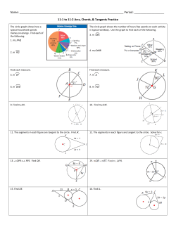


© Copyright 2026