Elements of Statistical Methods
2-Sample Location Problems (Ch 11)
Fritz Scholz
Spring Quarter 2010
May 18, 2010
The Basic 2-Sample Problem
It is assumed that we observe two independent random samples
X1, . . . , Xn1 iid ∼ P1
and Y1, . . . ,Yn2 iid ∼ P2
of continuous r.v.’s.
Let θ1 and θ2 be location parameters of P1 and P2, respectively.
For a meaningful comparison of such location parameters it makes sense to require
them to be of the same type, i.e., they should both be means (θ1 = µ1 = EXi and
θ2 = µ2 = EY j ) or both be medians (θ1 = q2(Xi) and θ2 = q2(Y j )).
∆ = θ1 − θ2 measures the difference in location between P1 and P2,
and such a difference is of main interest in the two sample problem.
The sample sizes n1 and n2 do not need to be the same, and there is
no implied pairing between the Xi and the Y j .
1
Sampling Awareness Questions
1. What are the experimental units, i.e., the objects being measured?
2. From what population(s) are the experimental units drawn?
3. What measurements were taken on each unit?
4. What random variables are relevant to a specific inference question?
2
Alzheimer’s Disease (AD) Study
The study purpose is to investigate the performance of AD patients in a
confrontation naming test relative to comparable non-AD patients.
60 mildly demented patients were selected, together with a “normal” control group
of 60, more or less matched (as a group) in age and other relevant characteristics.
Each was given the Boston Naming Test (BNT): high score = better performance.
1) Experimental unit is a person.
2) Experimental units belong to one of two populations:
AD patients and normal, comparable elderly persons.
3) One measurement (BNT score) per experimental unit.
4) Xi = BNT score for AD patient i, and Y j = BNT score for control subject j.
X1, . . . , X60 iid ∼ P1 and Y1, . . . ,Yn2 iid ∼ P2,
∆ = θ1 − θ2 = parameter of interest. Test H0 : ∆ ≥ 0 vs H1 : ∆ < 0.
3
Blood Pressure Medication
A drug is supposed to lower blood pressure.
n1 + n2 hypertensive patients are recruited for a double-blind study.
They are randomly divided into two groups of n1 and n2 patients,
the first group gets the drug the second group gets a look alike placebo.
Neither the patients nor the measuring technician know who gets what.
1) Experimental unit is a hypertensive patient.
2) Experimental unit belongs to one of two populations, a hypertensive population
that gets the drug and a hypertensive population that gets the placebo.
Randomization makes it possible to treat them as samples from the same set of
hypertensive patients. Each patient could come from either population (trick).
3) Two measurements (before and after treatment) on each experimental unit.
4
Blood Pressure Medication(continued)
4) B1i and A1i are the before and after blood pressure measurements on patient i
in the treatment group.
Similarly, B2i and A2i are the corresponding measurements for the control group.
Xi = B1i − A1i = decrease in blood pressure for patient i in the treatment group
Yi = B2i − A2i = decrease in blood pressure for patient i in the control group
X1, . . . , Xn1 iid ∼ P1
and
Y1, . . . ,Yn2 iid ∼ P2
Want to make inference about ∆ = θ1 − θ2. ∆ > 0 ⇐⇒ θ1 > θ2.
To show that the drug lowers the blood pressure more than the placebo
we want to test H0 : ∆ ≤ 0 against H1 : ∆ > 0.
We reject H0 when we have sufficient evidence for the drug’s effectiveness.
5
Two Important 2-Sample Location Problems
1. Assume that both sampled populations are normal
X ∼ P1 = N (µ1, σ21)
and
Y ∼ P2 = N (µ2, σ22)
This is referred to as the normal 2-sample location problem.
Normal shape, with possibly different means and standard deviations.
2. The two sampled populations give rise to continuous random variables
X and Y .
We assume that the two poulations differ only in the location of their median,
but are otherwise the same (same spread, same shape).
This is referred to as the general two-sample shift problem.
Same shape and variability, possible difference in locations (shift).
Here the median is the natural location parameter (it always exists).
6
The Normal 2-Sample Location Problem
The plug-in estimator of ∆ = µ1 − µ2 naturally is
∆ˆ = µˆ 1 − µˆ 2 = X¯ − Y¯
It is unbiased, since
E ∆ˆ = E(X¯ − Y¯ ) = E X¯ − EY¯ = µ1 − µ2 = ∆
∆ˆ is consistent, i.e.,
P
∆ˆ −→ ∆ as n1, n2 −→ ∞
∆ˆ is asymptotically efficient, i.e., best possible within the normal model.
7
The Distribution of X¯ − Y¯
In the context of the normal 2-sample problem we have from before
X¯ ∼ N
σ21
µ1,
n1
!
and
Y¯ ∼ N
σ22
µ2 ,
n2
!
Based on earlier results on sums of independent normal random variables
=⇒
∆ˆ = X¯ − Y¯ ∼ N
σ21 σ22
µ1 − µ2, +
n1 n2
!
=N
σ21 σ22
∆, +
n1
!
n2
We address three different situations for testing and confidence intervals:
1) σ1 and σ2 known. Rare but serves as stepping stone, exact solution.
2) σ1 and σ2 unknown, but σ1 = σ2 = σ. Ideal but rare, exact solution.
3) σ1 and σ2 unknown, but not assumed equal. Most common case in practice,
with good approximate solution.
8
Testing H0 : ∆ = ∆0 Against H1 : ∆ 6= ∆0
(σ1, σ2 Known)
Our previous treatment of the normal 1-sample problem suggests using
∆ˆ − ∆0
X¯ − Y¯ − ∆0
= r
Z=r
σ21
n1
σ22
+n
2
σ21
n1
as the appropriate test statistic.
σ22
+n
2
Reject H0 when |Z| ≥ qz, where qz is the 1 − α/2 quantile of N (0, 1).
When H0 is true, then Z ∼ N (0, 1) and we get
PH0 (|Z| ≥ qz) = α
the desired probability of type I error. If |z| denotes the observed value of |Z| then
the significance probability of |z| is
p(|z|) = PH0 (|Z| ≥ |z|) = 2Φ(−|z|) = 2 ∗ pnorm(−abs(z))
i.e., reject H0 at level α when p(|z|) ≤ α or |z| ≥ qz.
9
Confidence Intervals for ∆ (σ1, σ2 Known)
Again we can obtain (1 − α)-level confidence intervals for ∆ as consisting of all
values ∆0 for which the corresponding hypothesis H0 = H0(∆0) : ∆ = ∆0
cannot be rejected at significance level α. Or, more directly

s

σ21 σ22
+ 
1 − α = P(|Z| < qz) = P∆0 |∆ˆ − ∆0| < qz
n1 n2


s
s
σ21 σ22
σ21 σ22
= P∆0 −qz
+
< ∆0 − ∆ˆ < qz
+ 
n1 n2
n1 n2


s
s
σ21 σ22
σ21 σ22
= P∆0 ∆ˆ − qz
+
< ∆0 < ∆ˆ + qz
+ 
n1 n2
n1 n2
s
with desired (1 − α)-level confidence interval
ˆ
∆±q
z
σ21 σ22
+
n1 n2
which contains ∆0 if and only if p(|z|) > α or |z| < qz.
10
Example
Suppose we know σ1 = 5 and observe x¯ = 7.6 with n1 = 60 observations and
have σ2 = 2.5 and observe y¯ = 5.2 with n2 = 15 observations.
For a 95% confidence interval for ∆ = µ1 − µ2 we compute
=⇒
qz = qnorm(.975) = 1.959964 ≈ 1.96
s
52 2.52
(7.6 − 5.2) ± 1.96 ·
+
= 2.4 ± 1.79 = (0.61, 4.19)
60
15
Test H0 : ∆ = 0 against H1 : ∆ 6= 0 we find
(7.6 − 5.2) − 0
z=q
= 2.629
52/60 + 2.52/15
z(|z|) = P0(|Z| ≥ |2.629|) = 2 ∗ pnorm(−2.629) = 0.008563636 < 0.05
agreeing with the interval above not containing zero.
11
Estimating σ2 = σ21 = σ22
We have two estimates for the common unknown variance σ2
n1
1
¯ 2
(Xi − X)
S12 =
∑
n1 − 1 i=1
and
n2
1
S22 =
(Yi − Y¯ )2
∑
n2 − 1 i=1
Either one could be used in the standardization of a T statistic (not efficient).
Rather use the appropriate weighted average, the pooled sample variance
2 + (n − 1)S2
2
2
(n
−
1)S
(n
−
1)S
(n
−
1)S
1
2
1
2
2=
1
2=
1
2
SP
+
(n1 − 1) + (n2 − 1)
(n1 − 1) + (n2 − 1) (n1 − 1) + (n2 − 1)
2 = E
ESP
(n1 − 1)S12
(n1 − 1) + (n2 − 1)
!
+E
(n2 − 1)S22
!
(n1 − 1) + (n2 − 1)
(n1 − 1)ES12
(n2 − 1)ES22
=
+
(n1 − 1) + (n2 − 1) (n1 − 1) + (n2 − 1)
(n1 − 1)σ2
(n2 − 1)σ2
=
+
= σ2
(n1 − 1) + (n2 − 1) (n1 − 1) + (n2 − 1)
2 is unbiased
i.e., SP
12
2 when σ2 = σ2
More on SP
1
2
2 is a consistent and efficient estimator of σ2 .
SP
Recall
(n1 − 1)S12
2 (n − 1)
V1 =
∼
χ
1
σ2
and
(n2 − 1)S22
2 (n − 1)
V2 =
∼
χ
2
σ2
S12 and S22 are independent.
Previous results about sums of independent χ2 random variables
2
(n1 − 1)S12 (n2 − 1)S22
(n1 + n2 − 2)SP
2 (n + n − 2)
=⇒ V1 +V2 =
=
+
∼
χ
1
1
σ2
σ2
σ2
ˆ and S2 .
The independence of X¯ , Y¯ , S12 and S22 implies the independence of ∆
P
13
Standardization when σ21 = σ22
For testing H0 : ∆ = ∆0 against H1 : ∆ 6= ∆0 we use
T = r
∆ˆ − ∆0
1 + 1 S2
P
n1 n2
= r
∆ˆ − ∆0
1
1 + 1 σ2
n1 n2
q
2 1
SP
2
=q
σ
Z
V1 +V2
n1 +n2 −2
When ∆ = ∆0, then
Z = r
∆ˆ − ∆0
∼ N (0, 1)
and
V1 +V2 = χ2(n1 + n2 − 2)
1
1
2
n1 + n2 σ
Z and V1 +V2 are independent of each other and thus under H0 : ∆ = ∆0
T ∼ t(n1 + n2 − 2), by definition of the Student t distribution.
14
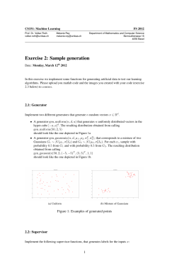
Testing H0 : ∆ = ∆0 Against H1 : ∆ 6= ∆0
(σ1, σ2 Unknown)
Of course, we reject H0 when the observed value |t| of |T | is too large.
The significance probability of |t| is
p(|t|) = PH0 (|T | ≥ |t|) = 2PH0 (T ≤ −|t|) = 2 ∗ pt(−abs(t), n1 + n2 − 2)
Again note that p(|t|) ≤ α ⇐⇒ |t| ≥ qt ,
where qt is the (1 − α/2)-quantile of the t(n1 + n2 − 2) distribution.
0.0
0.2
α 2
−4
− t
− qt
α 2
−2
0
2
qt
t
4
15
Standard Error
The standard error of an estimator is its estimated standard deviation.
√
¯
The standard error of X is S/ n when σ is unknown and estimated by S.
√
¯
When σ is known the standard error of X is σ/ n. (nothing to estimate)
p
ˆ
The standard error of ∆ when σ1 = σ2 = σ is unknown is SP 1/n1 + 1/n2.
p
When σ1 = σ2 = σ is known it is σ 1/n1 + 1/n2. (nothing to estimate)
Note that our test statistics in Z or T form always look like
estimator − hypothesized mean of estimator
standard error of the estimator
16
Confidence Interval for ∆ when σ21 = σ22
Let qt = qt (1 − α/2) denote the (1 − α/2)-quantile of t(n1 + n2 − 2).
Then for any ∆0


 ∆ˆ − ∆ 


0
1 − α = P∆0 (|T | < qt ) = P∆0  r
<
q

t


1 + 1 S2
P
n1 n2


s
s
1
1
1
1
2
2
ˆ
ˆ

= P∆0 ∆ − qt
+
SP < ∆0 < ∆ + qt
+
SP
n1 n2
n1 n2
=⇒
∆ˆ ± qt
s
1
1
2
SP
+
n1 n2
ˆ and SP)
(a random interval through ∆
is a (1 − α)-level confidence interval for ∆.
Again it consists of all acceptable ∆0 when testing H0 : ∆ = ∆0 against H1 : ∆ 6= ∆0.
17
Example (continued)
In our previous example instead of known σ’s assume that s1 = 5 and s2 = 2.5.
Inspite of this discrepancy in s1 and s2 assume that σ1 = σ2.
59 · 52 + 14 · 2.52
2
sP =
= 21.40411
59 + 14
For a 95% confidence interval we compute qt = qt(.975, 73) = 1.992997 ≈ 1.993
=⇒
(7.6−5.2)±1.993·
p
21.40411 · (1/60 + 1/15) = 2.4±2.66 = (−0.26, 5.06)
For testing H0 : ∆ = 0 against H1 : ∆ 6= 0 we find
t=p
with
(7.6 − 5.2) − 0
≈ 1.797
21.40411 · (1/60 + 1/15)
p(|t|) = P0(|T | ≥ |1.797|) = 2 ∗ pt(−1.797, 73) = 0.07647185 > 0.05
agreeing with the inference from the confidence interval.
18
σ1, σ2 Unknown, But Not Necessarily Equal
Under H0 : ∆ = ∆0
Z = q
but
TW = q
∆ˆ − ∆0
σ21/n1 + σ22/n2
∆ˆ − ∆0
∼ N (0, 1)
∼ ???
S12/n1 + S22/n2
Welch (using Satterthwaite’s approximation) argued that TW ≈ t(ν) with
ν=
[σ21/n1 + σ22/n2]2
(σ21 /n1 )2 (σ22 /n2 )2
n1 −1 + n2 −1
estimated by νˆ =
[s21/n1 + s22/n2]2
(s21 /n1 )2 (s22 /n2 )2
n1 −1 + n2 −1
provides good approximate significance probabilities and confidence intervals
when using t(νˆ ) in the calculation of p(|t|) and qt .
Fractional values of νˆ present no problem in qt and pt.
This has been explored via simulation with good results in coverage
and false rejection rates for a wide range of (σ1, σ2)-scenarios.
19
Example (continued)
vˆ =
[52/60 + 2.52/15]2
(52 /60)2
60−1 +
(2.52 /15)2
= 45.26027 ≈ 45.26
15−1
For a 95% confidence interval we compute
qt = qt(.975, 45.26) = 2.013784 ≈ 2.014 and get
q
(7.6 − 5.2) ± 2.014 · 52/60 + 2.52/15 = 2.4 ± 1.84 = (0.56, 4.24)
For testing H0 : ∆ = 0 against H1 : ∆ 6= 0 we get
(7.6 − 5.2) − 0
tW = q
≈ 2.629
52/60 + 2.52/15
p(|tW |) = P0(|TW | ≥ |tW |) ≈ 2 ∗ pt(−2.629, 45.26) = 0.01165687 < 0.05
Note the difference in results to when we assumed σ1 = σ2.
20
Comments on Using Student’s t -Test
• if n1 = n2 then t = tW (verify by simple algebra).
• If the population variances (and hence the sample variances) tend to be
approximately equal, then t and tW tend to be approximately equal.
• If the larger sample is drawn from the population with the larger variance,
then |t| will tend to be less than |tW |.
All else equal, Student’s t -test will give inflated significance probabilities.
• If the larger sample is drawn from the population with the smaller variance,
then |t| will tend to be larger than |tW |.
All else equal, Student’s t -test will give understated significance probabilities.
Don’t use Student’s t -test, use tW with νˆ instead.
21
TW Test for Large Samples
Again we can appeal to large sample results to claim
P
S12 −→ σ21 ,
P
S22 −→ σ22
and
TW ≈ N (0, 1)
These limiting results hold even when the sampled distributions are not normal,
as long as the variances σ21 and σ22 exist and are finite.
Just use the N (0, 1) distribution to calculate approximate significance probabilities
for testing H0 : ∆ = µ1 − µ2 = ∆0 against H1 : ∆ 6= ∆0
PH0 (|TW | ≥ |tW |) ≈ 2 ∗ pnorm(−abs(tW))
Use qz = qt(1 − α/2) in place of qt for ≈ (1 − α)-level confidence intervals
s
∆ˆ ± qz ·
s21 s22
+
n1 n2
22
2-Sample Shift Problem
Definition: A family of distributions P = {Pθ : θ ∈ R } is a shift family iff
X ∼ Pθ
=⇒
X0 = X − θ ∼ P0
=⇒
X = X0 + θ ∼ Pθ
Example: For fixed σ2 the family {N (θ, σ2) : θ ∈ R } is a shift family.
The 2-sample location problem started with 2 normal shift families with common
variance. We relaxed that to unequal variances, but kept the normality assumption.
Relax this in the other direction:
Let P0 denote the family of all continuous distributions on R with median 0.
For any P0 ∈ P0 we take as our shift family PP0 = {Pθ : θ ∈ R , Pθ=0 = P0}.
The extra P0 in the notation indicates which distribution shape is shifted around.
We observe two independent random samples
X1, . . . , Xn1 ∼ Pθ1 ∈ PP0
and
Y1, . . . ,Yn2 ∼ Pθ2 ∈ PP0
They arise from the same shape P0 with possibly different shifts.
We wish to make inferences about ∆ = θ1 − θ2.
23
Testing in the 2-Sample Shift Problem
Test H0 : ∆ = 0 against H1 : ∆ 6= 0. The case H0 : ∆ = ∆0 against H1 : ∆ 6= ∆0
can be reduced to the previous case by subtracting ∆0 from the X -sample:
Xi0 = Xi − ∆0 ∼ Pθ1−∆0 = Pθ0
1
∆0 = θ01 − θ2 = θ1 − ∆0 − θ2 = 0 ⇐⇒ ∆ = θ1 − θ2 = ∆0
Since the distributions of the X ’s and Y ’s are continuous, they have n1 + n2 = N
distinct values with probability 1.
Rank the (assumed distinct) values in the pooled sample of N observations, e.g.,
X3 gets rank 5 iff X3 is the 5th in the ordered sequence of N pooled sample values,
Y6 gets rank 1 if it is is the smallest of all N pooled values.
Let Tx be the sum of the X -sample ranks and Ty be the sum of the Y -sample ranks.
N
Tx + Ty =
∑ k = N(N + 1)/2
k=1
24
Null Distribution of the Wilcoxon Rank Sum
Under H0 : ∆ = 0 both samples come from the same continuous distribution Pθ.
We may view the sampling process as follows: Select N values Z1, . . . , ZN iid Pθ.
Out of Z1, . . . , ZN randomly select n1 as the X -sample, the remainder being
the Y -sample.
N
All n X -sample selections (and corresponding rank sets) are equally likely.
1
Some of these rank sets will give the same Tx .
By enumerating all rank sets (choices of n1 numbers from 1, 2, . . . , N ) it is in
principle possible to get the null distribution of Tx .
Naturally, we would reject H0 when Tx is either too high or too low.
This is the Wilcoxon Rank Sum Test.
Significance probabilities are computed from the null distribution of Tx .
25
Using rank and combn
> x <-c(9.1,8.3); y <- c(11.9,10.0,10.5,11.3)
> rank(c(x,y)) # ranking the pooled samples
[1] 2 1 6 3 4 5 # Tx = 2+1 = 3
> combn(1:6,2) # all sets of 2 taken from 1,2,...,6
[,1] [,2] [,3] [,4] [,5] [,6] [,7] [,8]
[1,]
1
1
1
1
1
2
2
2
[2,]
2
3
4
5
6
3
4
5
[,9] [,10] [,11] [,12] [,13] [,14] [,15]
[1,]
2
3
3
3
4
4
5
[2,]
6
4
5
6
5
6
6
> combn(1:6,2,FUN=sum) # sum of those 15 = choose(6,2) sets of 2
[1] 3 4 5 6 7 5 6 7 8 7 8 9 9 10 11
> table(combn(1:6,2,FUN=sum)) # tabulate distict sums with frequencies
3 4 5 6 7 8 9 10 11
1 1 2 2 3 2 2 1 1 # null distribution is symmetric around 7
Significance probability is 2 · 1/15 = 0.1333333 > 0.05
mean(abs(combn(1 : 6, 2, FUN = sum) − 7) >= abs(3 − 7)) = 0.1333333
26
Symmetry of Tx Null Distribution
The null distribution of Tx is symmetric around n1(N + 1)/2 = E0Tx
with variance var0(Tx ) = n1n2(N + 1)2/12.
Let Ri and R0i = N + 1 − Ri be the Xi rankings in increasing and decreasing order.
n1
Tx =
∑ Ri
and
Tx0 =
i=1
n1
n1
i=1
i=1
∑ R0i = ∑ (N + 1 − Ri) = n1(N + 1) − Tx
Tx and Tx0 have the same distribution, being sums of n1 ranks randomly chosen
from 1, 2, . . . , N .
D
Using = to denote equality in distribution we have
n1(N + 1) D n1(N + 1)
=
− Tx
=⇒ Tx −
2
2
n (N + 1)
n (N + 1)
P0 Tx = 1
+x
= P0 Tx − 1
=x
2
2
n (N + 1)
n (N + 1)
= P0 1
− Tx = x = P0 Tx = 1
−x
2
2
D
Tx = Tx0 = n1(N + 1) − Tx
27
The Mann-Whitney Test Statistic
Let X(1) < . . . < X(n1) be the ~
X sample in increasing order.
Let Rk denote the rank of X(k) in the pooled sample. Then
n
o
Rk = k + # Y j : Y j < X(k)
and
n1
n1
n1
n
o n (n + 1)
Tx = ∑ Rk = ∑ k + ∑ # Y j : Y j < X(k) = 1 1
+WY X
2
k=1
k=1
k=1
where n1(n1 + 1)/2 = 1 + . . . + n1 is the smallest possible value for Tx and
WY X = # (Xi,Y j ) : Y j < Xi
Since Tx = WY X −
is the Mann-Whitney test statistic
n1 (n1 +1)
the test can be carried out using either test statistic.
2
The value set of WY X is 0 (no Y j < any Xi),1, 2, . . . , n1 · n2 (all Y j < all Xi).
The distribution of WY X is symmetric around n1 · n2/2.
28
Four Approaches to the Null Distribution
1. Null distribution using explicit enumeration via combn
2. Null distribution using the R function pwilcox
3. Null distribution using simulation
4. Null distribution using normal approximation
29
Null Distribution Using combn
1. Exact null distribution of Tx via combn, for choose(n1+n2,n1) not too large
P0(Tx ≤ tx) = mean(combn(n1 + n2, n1, FUN = sum) <= tx)
n
(N
+
1)
n
(N
+
1)
1
1
p(tx) = P0 Tx −
≥ tx −
2
2
= 2 ∗ mean(abs(combn(n1 + n2, n1, FUN = sum) − n1 ∗ (N + 1)/2)
<= −abs(tx − n1 ∗ (N + 1)/2))
30
Null Distribution Using pwilcox
2. R has a function pwilcox that efficiently calculates
P0(Tx ≤ tx) = P0(WY X ≤ tx − n1 ∗ (n1 + 1)/2)
= pwilcox(tx − n1 ∗ (n1 + 1)/2, n1, n2)
n1(N + 1) n1(N + 1) p(tx) = P0 Tx −
≥ tx −
2
2
n1(N + 1)
n
(N
+
1)
1
= 2P0 Tx −
≤ − tx −
2
2
= 2 ∗ pwilcox(−abs(tx − n1 ∗ (N + 1)/2)
−n1 ∗ (n1 + 1)/2 + n1 ∗ (N + 1)/2, n1, n2)
31
Null Distribution Using Simulation
3. It is easy to simulate random samples of n1 ranks taken from 1, 2, . . . , n1 + n2
N <- n1+n2; Nsim <- 10000; Tx.sim <- numeric(Nsim)
for(i in 1:Nsim){ Tx.sum[i] <- sum(sample(1:N,n1))}
n1(N + 1) n1(N + 1) ≥ tx −
p(tx) = P0 Tx −
2
2
≈ mean(abs(Tx.sim − n1 ∗ (N + 1)/2) >= abs(tx − n1 ∗ (N + 1)/2))
The accuracy of this approximation is completely controlled by Nsim (LLN).
See also the function W2.p.sim <- function(n1,n2,tx,draws=1000){...}
given as part of shift.R on the text book web site. (draws=Nsim)
32
Null Distribution Using Normal Approximation
4. The normal approximation, good for larger sample sizes n1 and n2, gives
Tx − E0Tx
tx − E0Tx
P0 (Tx ≤ tx) = P0 p
≤p
var0(Tx)
var0(Tx)


!
tx − E0Tx
≈Φ p
var0(Tx)
!
 tx − n1(N + 1)/2 
= Φ q

2
n1n2(N+1)
12
= pnorm((tx − n1 ∗ (N + 1)/2)/sqrt(n1 ∗ n2 ∗ (N + 1)ˆ2/12))
n
(N
+
1)
n
(N
+
1)
1
1
≥ tx −
p(tx) = P0 Tx −
2
2
≈ 2 ∗ pnorm(−abs(tx − n1 ∗ (N + 1)/2)/sqrt(n1 ∗ n2 ∗ (N + 1)ˆ2/12))
See also W2.p.norm <- function(n1,n2,tx) {...}
given as part of shift.R on the text book web site.
33
Example
For our previous example, where we illustrated complete enumeration via combn,
we had
P0(|Tx − 7| ≥ |3 − 7|) =
2
≈ 0.1333
15
Using pwilcox we get
> 2*pwilcox(-abs(3-2*7/2)-2*3/2+2*7/2,2,4)
[1] 0.1333333
In 5 applications of W2.p.sim(2,4,3) we get: 0.135, 0.114, 0.110, 0.114, 0.151,
W2.p.norm(2,4,3)=0.1051925, reasonably close for such small sample sizes.
34
The Case of Ties
When there are ties in the pooled sample we add tiny random amounts to the
sample values to break the ties.
Then compute the significance probability for each such breaking of ties.
Repeat this process many times and average all these significance probabilities.
Alternatively, compute the significance probabilities for the breaking of ties
least (or most) in favor of H0 and base decisions on these two extreme cases.
We could also use complete enumeration or simulation while working with the
pooled vector of midranks returned by rz <- rank(c(x,y)) and then use
combn(rz,n1,FUN=sum) to get all possible midrank sums.
From that get the exact significance probability, conditional on the tie pattern.
Observations tied at ranks 6, 7, 8 and 9 get midrank 7.5 each.
35
Example with Ties
~x
6.6
14.7
15.7
11.1
7.0
9.0
9.6
8.2
6.8
7.2
~y
4.2
3.6
2.3
2.4
13.4
1.3
2.0
2.9
8.8
3.8
Test H0 : ∆ = 3 versus H1 : ∆ 6= 3 at α = 0.05. Replacing xi by xi0 = xi − 3 and
assigning the pooled ranks
> c(x0-3,y0)
[1] 3.6 11.7 12.7 8.1 4.0 6.0 6.6 5.2 3.8 4.2
[11] 4.2 3.6 2.3 2.4 13.4 1.3 2.0 2.9 8.8 3.8
> rz <- rank(c(x0-3,y0)); rz
[1] 6.0 18.0 19.0 16.0 10.0 14.0 15.0 13.0 8.5 11.5
[11] 11.5 7.0 3.0 4.0 20.0 1.0 2.0 5.0 17.0 8.5
> sort(c(x0-3,y0))
[1] 1.3 2.0 2.3 2.4 2.9 3.6 3.6 3.8 3.8 4.0
[11] 4.2 4.2 5.2 6.0 6.6 8.1 8.8 11.7 12.7 13.4
We recognize three pairs of tied values (3.6, 3.6), (3.8, 3.8) and (4.2, 4.2),
receiving respective midranks (6, 7) (???), (8.5, 8.5) and (11.5, 11.5).
36
What Happened to Midrank 6.5?
> x0[1]-3==3.6
[1] FALSE
> x0[1]-3-3.6
[1] -4.440892e-16
> y0[2]==3.6
[1] TRUE
> round(x0[1]-3,1)==3.6
[1] TRUE
> round(x0[1]-3,1)-3.6
[1] 0
> rank(c(round(x0-3,1),y0))
[1] 6.5 18.0 19.0 16.0 10.0 14.0 15.0 13.0 8.5 11.5
[11] 11.5 6.5 3.0 4.0 20.0 1.0 2.0 5.0 17.0 8.5
Computer arithmetic is done in binary form and it sometimes produces surprises.
If we are aware of this we can avoid it as above by a proper rounding procedure.
37
Significance Probability
Using the fix we have a midrank sum of
tx = sum(rank(c(round(x0 − 3, 1), y0))[1 : 10]) = 131.5
Depending on how the ties are broken, tx could have taken values as low as 130
and as high as 133.
Comparing 130 and 133 with n1(N + 1)/2 = 105 it would give us
p(130) = P0(|Tx − 105| ≥ |130 − 105|) = 2 · P0(Tx ≤ 105 − 25) = 2 · P0(Tx ≤ 80)
= 2 ∗ pwilcox(80 − n1 ∗ (n1 + 1)/2, n1, n2) = 0.06301284
p(133) = P0(|Tx − 105| ≥ |133 − 105|) = 2 · P0(Tx ≤ 105 − 28) = 2 · P0(Tx ≤ 77)
= 2 ∗ pwilcox(77 − n1 ∗ (n1 + 1)/2, n1, n2) = 0.03546299
Not sufficiently strong evidence against H0 at level α = 0.05.
38
Using W2.p.sim and W2.p.norm
Instead of using pwilcox we could, as suggested in the text, also use W2.p.sim
or W2.norm to get the significance probabilities of tx=130 and tx=133.
> W2.p.sim(10,10,130,10000)
[1] 0.0662
> W2.p.sim(10,10,133,10000)
[1] 0.037
> W2.p.norm(10,10,130)
[1] 0.0640221
> W2.p.norm(10,10,133)
[1] 0.03763531
Note the quality of these two approximations.
39
Significance Probability
Since choose(20, 10) = 184756 we can dare to compute all possible midrank
sums of 10 taken from the above set of 20 midranks.
We want to assess the significance probability of tx = 131.5 in relation to the
average of all pooled midranks. That average is again 105. Thus
p(131.5) = mean(abs(combn(rz, 10, FUN = sum) − 105) >= abs(131.5 − 105))
= 0.04523804
This is barely significant at level α = 0.05, i.e., we should reject H0 : ∆ = 3
when testing it against H1 : ∆ 6= 3.
On the other hand, averaging many simulated random breaking of ties we get
> W2.p.ties(x0,y0,3,100000)
[1] 0.05412
40
Point Estimation of ∆
Following our previous paradigm, we should use that value ∆0 as estimate of ∆
which makes the hypothesis H0 : ∆ = ∆0 least rejectable.
This would be that ∆0 for which the rank sum Tx (∆0) of the Xi0 = Xi − ∆0
comes closest to the center n1(N + 1)/2 of the null distribution.
recall the equivalent form Tx (∆0) = WY X 0 −
n (n + 1)
n1(n1 + 1)
= WY,X−∆0 − 1 1
2
2
WY,X−∆0 = #{(Xi0,Y j ) : Y j < Xi0} = #{(X − ∆0,Y j ) : Y j < Xi − ∆0}
n2n2
= #{(Xi,Y j ) : ∆0 < Xi −Y j } =
= center of the W null distribution
2
when ∆0 = median{Xi −Y j : i = 1, . . . , n1, j = 1, . . . , n2}.
e = median(Xi −Y j ) is also known as the Hodges-Lehmann estimator of ∆.
∆
As in interesting contrast compare it with this alternate form of X¯ − Y¯
n1
n2
n1 n2
1
1
1
∆ˆ = X¯ − Y¯ =
Xi −
Yj =
(Xi −Y j )
∑
∑
∑
∑
n1 i=1
n2 j=1
n1n2 i=1 j=1
41
e
Computation of ∆
e can be computed by using W2.hl, see shift.R on the text book web site.
∆
> W2.hl(x0,y0)
[1] 5.2
or alternatively
> median(outer(x0,y0,"-"))
[1] 5.2
where outer produces a matrix of all pairwise operations "-" on the input vectors.
> outer(1:3,3:2,"-")
[,1] [,2]
[1,]
-2
-1
[2,]
-1
0
[3,]
0
1
42
Set Estimation of ∆
By the well practiced paradigm, the confidence set consists of all those ∆0 for which
we cannot reject H0 : ∆ = ∆0 at level α when testing it against H1 : ∆ 6= ∆0.
We accept H0 whenever k ≤ WY,X−∆0 ≤ n1n2 − k = M − k, where the integers
k = 1, 2, 3, . . . ≤ (M + 1)/2 govern the achievable significance levels αk
αk = 2P∆0 (WY,X−∆0 ≤ k − 1) = 2P0(WY X ≤ k − 1)
With probability 1 all the M = n1 · n2 differences Di j = Xi −Y j are distinct.
Denote their ordered sequence by D(1) < D(2) < . . . < D(M) and note
k ≤ WY,X−∆0 = #{(Xi − ∆0,Y j ) : Y j < Xi − ∆0} = #{(Xi,Y j ) : ∆0 < Xi −Y j }
⇐⇒ D(M−k+1) > ∆0.
(using a = M − k)
Similarly, WY,X−∆0 ≤ a ⇐⇒ D(M−a) ≤ ∆0. Thus
WY,X−∆0 ≤ M −k ⇐⇒ D(k) ≤ ∆0
[D(k), D(M−k+1)] is our (1 − αk )-level confidence interval for ∆.
We can use exact calculation (pwilcox), simulation approximation or normal
approximation to get the appropriate (k, αk ) combination.
43
Confidence Interval for ∆: Example
For the previous example of 10 and 10 obs. get a 90% confidence interval for ∆.
k = qwilcox(1 − 0.05/2, 10, 10) = 72 = smallest k such P0(WY X ≤ k) ≥ 0.95.
In fact, pwilcox(72, 10, 10) = 0.9553952 and pwilcox(71, 10, 10) = 0.9474388
P0(WY X ≥ 73) = 1 − 0.9553952 = 0.0446048 = P0(WY X ≤ 27) = α28/2
[D(28), D(73)] = [3.4, 7.2]
is a 1 − α28 = 0.9108 level confidence interval for ∆
P0(WY X ≥ 72) = 1 − 0.9474388 = 0.0525612 = P0(WY X ≤ 28) = α29/2
[D(29), D(72)] = [3.4, 7.0]
is a 1 − α29 = 0.8949 level confidence interval for ∆
We apparently have ties among the Di j , since D(28) = D(29) = 3.4.
44
Using W2.ci in Example
The text explains how to use the normal approximation for finding a range of
k values such that P0(WY X ≤ k) ≈ α/2 and uses simulation to get a better
approximation to the actual P0(WY X ≤ k) for each of these k values.
This is implemented in the function W2.ci provided in shift.R.
> W2.ci(x0,y0,.1,10000)
k Lower Upper Coverage
[1,] 27
3.2
7.3
0.9261
[2,] 28
3.4
7.2
0.9115
[3,] 29
3.4
7.0
0.8944
[4,] 30
3.6
6.9
0.8728
[5,] 31
3.7
6.9
0.8615
This agrees fairly well with our intervals based on exact calculations.
45
How to Deal With Rounding
In our example we observed ties.
Such ties often are due to rounding data that are intrinsically of continuous nature.
Rounding confines the reported data to a grid of values consisting of 0, ±ε, ±2ε, ±3ε, . . . .
Let X 0 denote the continuous data value corresponding to the rounded value X .
=⇒ |X − X 0| ≤ ε/2 and |Di j − D0i j | = |Xi −Y j + Xi0 −Y j0| ≤ ε/2 + ε/2 = ε
=⇒ D(i) − ε ≤ D0(i) ≤ D(i) + ε
Since our confidence procedure is correct in terms of truly continuous data, i.e.,
P∆(∆ ∈ [D0(k), D0(M−k+1)]) = 1 − αk ,
we can view [D(k) − ε, D(M−k+1) + ε]
as a proper confidence interval for ∆ with confidence level
P∆(∆ ∈ [D(k) − ε, D(M−k+1) + ε]) ≥ P∆(∆ ∈ [D0(k), D0(M−k+1)]) = 1 − αk
46