IERG5290 Network Coding Theory
Lecture 0 - 07/01/2014
A Sample of Scribe Note – Pagerank algorithm
Lecturer: Kenneth Shum
Scribe: K. Shum
The Pagerank algorithm was invented by Page and Brin around 1998 and used in the prototype of
Google’s search engine. The objective is to estimate the popularity, or the importance, of a webpage, based
on the interconnection of the web. The rationale behind it is (i) a page with more incoming links is more
important than a page with less incoming links, (ii) a page with a link from a page which is known to be of
high importance is also important.
In this note, we study the convergence of the Pagerank algorithm from matrix’s point of view. In practice
the number of web pages is huge. In this notes, only examples of small size will be given.
1
Simplified Pagerank algorithm
The connections between pages is represented by a graph. A node represents a webpage and an arrow from
page A to page B means that there is a link from page A to page B. The number of out-going links is an
important parameter. We use the notation “out-degree of a node” to stand for the number of out-going links
contained in a page. This graph is usually referred to as the web graph. Each node in the graph is identiﬁed
with a page. We will use the term “node” and “page” interchangeably.
We following the notations in the wikipedia page for the Pagerank algorithm and let L(p) be the number
of out-going links in a page p (http://en.wikipedia.org/wiki/PageRank).
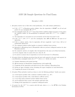
Example 1: There are four pages. Page A contains a link to page B, a link to page C, and a link to page
D. Page B contains one single link to page D. Page C points to pages A and D, and page D points to pages
A and C. They are represented by the following graph. We have L(A) = 3, L(B) = 1 and L(C) = L(D) = 2.
Let N be the total number of pages. We create an N × N matrix A by deﬁning the (i, j)-entry as
{
1
if there is a link from j to i,
aij = L(j)
0
otherwise.
In Example 1, the matrix A is the 4 × 4 matrix


0 0 1/2 1/2
1/3 0
0
0 

.
1/3 0
0
1/2
1/3 1 1/2 0
1
Note that the sum of the entries in each column is equal to 1.
In general, a matrix is said to be column-stochastic if the entries are non-negative and the sum of the
entries in each column is equal to 1. The matrix A is by design a column-stochastic matrix, provided that
each page contains at least one out-going link.
The simpliﬁed Pagerank algorithm is:
Initialize x to an N ×1 column vector with non-negative components, and then repeatedly replace
x by the product Ax until it converges.
We call the vector x the pagerank vector. Usually, we initialize it to a column vector whose components
are equal to each other.
We can imagine a bored surfer who clicks the links in a random manner. If there are k links in the page,
he/she simply picks one of the links randomly and goes the selected page. After a suﬃciently long time, the
N components of the pagerank vector are directly proportional to the number of times this surfer visits the
N web pages.
For example, in Example 1, we let the components of the vector x be xA , xB , xC and xD . Initialize x to
be the all-one column vector, i.e.,
   
xA
1
xB  1
  
x=
 xC  = 1 .
xD
1
The evolution of the pagerank vector is shown in the following table.
iteration
0
1
2
3
4
5
6
7
xA
1
1
1.3333
1.667
1.1944
1.2083
1.1968
1.2002
xB
1
0.3333
0.3333
.4444
0.3889
0.3981
0.4028
0.3989
xC
1
0.8333
1.25
.9861
1.0903
1.0613
1.0689
1.0647
xD
1
1.8333
1.0833
1.4028
1.3264
1.3322
1.3316
1.3361
We observe that the algorithm converges quickly in this example. Within 10 iterations, we can see that page
D has the highest rank. In fact, page D has 3 incoming links, while the others have either 1 or 2 incoming
links. It conforms with the rationale of the pagerank algorithm that a page with larger incoming links has
higher importance.
2
How to handle dangling node
A node is called a dangling node if it does not contain any out-going link, i.e., if the out-degree is zero. For
instance, node D in the next example is a dangling node.
Example 2:
2

0 0 1/2 0
1/3 0
0
0

.
1/3 0
0
0
1/3 1 1/2 0
We note that the entries in the last column are all zero, hence this matrix is not column-stochastic.
The simpliﬁed Pagerank algorithm collapses if there is dangling node in the web graph. As an example,
if we initialize the vector x to the all-one vector, the simpliﬁed Pagerank algorithm gives
The associated matrix A is

iteration
xA
xB
xC
xD
0
1
1
1
1
1
0.5
0.3333 0.8333 1.8333
2
0.1667 0.1667 0.1667 0.6667
3
0.0833 0.0556 0.0556 0.3056
4
0.0278 0.0278 0.0278 0.1111
5
0.0139 0.0093 0.0098 0.0509
The pagerank vector will converge to zero ultimately.
One remedy is to modify the simpliﬁed Pagerank algorithm by replacing any all-zero column by


1/N
1/N 


 ..  .
 . 
1/N
This adjustment is justiﬁed by modeling the behaviour of a web surfer, who after reading a page with no
out-going link, he/she will jump to a random page. He/she simply picks one of the N pages randomly with
equal probability. This model may not be realistic, but it simpliﬁes the computation of the algorithm.
¯ whose column is the same as A except the columns corresponding
In matrix format, we create a matrix A,
¯ by
to the dangling pages. Formally, we deﬁne the entries of matrix A

1

 L(j) if there is a link from node j to node i,
1
a
¯ij = N
if node j is a dangling node,


0
otherwise,
where N is the total number of pages.
¯ is
In Example 2, the matrix A

0
1/3

1/3
1/3
0 1/2
0
0
0
0
1 1/2
3

1/4
1/4
.
1/4
1/4
¯
In the Pagerank algorithm, we use A
¯ we get
use A,
iteration
0
1
2
3
4
5
¯ instead. In Example 2, if we
instead of A, and replace x by Ax
xA
1
0.75
0.8125
0.7969
0.8008
0.7998
xB
1
0.5833
0.7708
0.6823
0.7253
0.7041
xC
1
0.5833
0.7708
0.6823
0.7253
0.7041
xD
1
2.0833
1.6458
1.8385
1.7487
1.7920
We see that page D has the highest ranking.
3
How to handle reducible web graph
Consider the following web graph consisting of eight web pages.
Example 3:
There is no dangling node. But, once a surfer arrives at pages E, F, G or H, he/she will get stuck in these
four pages. The matrix A of this web graph is


0
0
1/2
0
0
0
0
0
1/3
0
0
1/2 0
0
0
0 


1/3
0
0
0
0
0
0
0 


1/3 1/2 1/2
0
0
0
0
0 


 0 1/2 0
0
0 1/2 0
0 


 0
0
0
0
0
0
1 1/2


 0
0
0
1/2 1
0
0 1/2
0
0
0
0
0 1/2 0
0
If we initialize the pagerank vector x to be the 8 × 1 column vector with components all equal to 1/8,
then the Pagerank algorithm gives
iteration
0
1
2
3
4
5
6
7
8
xA
0.125
0.0625
0.0208
0.0104
0.0035
0.0017
0.0006
0.0003
0.0001
xB
0.125
0.1042
0.1042
0.0538
0.0382
0.0181
0.0116
0.0053
0.0032
xC
0.125
0.0417
0.0208
0.0069
0.0035
0.0012
0.0006
0.0002
0.0001
xD
0.125
0.1667
0.0937
0.0697
0.0339
0.0220
0.0102
0.0063
0.0028
4
xE
0.125
0.125
0.1458
0.1927
0.1701
0.1740
0.1937
0.1739
0.1801
xF
0.125
0.1875
0.2813
0.2865
0.3099
0.3694
0.3362
0.3549
0.3752
xG
0.125
0.25
0.2396
0.2396
0.2977
0.2587
0.2625
0.2912
0.2610
xH
0.125
0.0625
0.0938
0.1406
0.1432
0.1549
0.1847
0.1681
0.1774
We can see that the ranking of pages A to D drop to zero eventually. But page D has three incoming links
and should have some nonzero importance. The Pagerank algorithm does not work in this example.
This pathological web graph belongs to the category of reducible graph. In general, a graph is called
irreducible if for any pair of distinct nodes, we can start from one of them, follow the links in the web graph
and arrive at the other node, and vice versa. A graph which is not irreducible is called reducible. In Example
3, there is no path from E to B, and no path from G to D. The graph is therefore reducible.
In order to calculate page ranks properly for a reducible web graph, Page and Brin proposed that take
¯ with an all-one N × N matrix. Deﬁne the matrix
a weighted average of the matrix A


1 1 1 ... 1
1 1 1 . . . 1

¯ + 1−d
M = dA
. . .
.
N  .. .. .. . . . .. 
1 1 1 ... 1
¯ is the modiﬁed matrix deﬁned in the previous section, and d is
where A
constant d is usually called the damping factor or the damping constant.
Google.
With d set to 0.85, the matrix M for the web graph in Example 3 is

0.0187 0.0187 0.4437 0.0187 0.0187 0.0187
0.3021 0.0187 0.0187 0.4437 0.0187 0.0187

0.3021 0.0187 0.0187 0.0187 0.0187 0.0187

0.3021 0.4437 0.4437 0.0187 0.0187 0.0187
M=
0.0187 0.4437 0.0187 0.0187 0.0187 0.4437

0.0187 0.0187 0.0187 0.0187 0.0187 0.0187

0.0187 0.0187 0.0187 0.4437 0.8688 0.0187
0.0187 0.0187 0.0187 0.0187 0.0187 0.4437
a number between 0 and 1. The
The default value of d is 0.85 in
0.0187
0.0187
0.0187
0.0187
0.0187
0.8688
0.0187
0.0187

0.0187
0.0187

0.0187

0.0187

0.0187

0.4437

0.4437
0.0187
Using this matrix in each iteration, the evolution of the pagerank vector is
iteration
0
1
2
3
4
5
6
7
8
xA
0.125
0.0719
0.0418
0.0354
0.0317
0.0310
0.0305
0.0304
0.0304
xB
0.125
0.1073
0.1073
0.0764
0.0682
0.0593
0.0568
0.0548
0.0543
xC
0.125
0.0542
0.0391
0.0306
0.0288
0.0277
0.0275
0.0274
0.0274
xD
0.125
0.1604
0.1077
0.0928
0.0742
0.0690
0.0645
0.0633
0.0623
xE
0.125
0.1250
0.1401
0.1688
0.1571
0.1588
0.1662
0.1598
0.1615
xF
0.125
0.1781
0.2459
0.2491
0.2613
0.2877
0.2752
0.2811
0.2867
xG
0.125
0.2313
0.2237
0.2237
0.2541
0.2368
0.2382
0.2474
0.2392
xH
0.125
0.0719
0.0945
0.1232
0.1246
0.1298
0.1410
0.1357
0.1382
We see that the page ranks of pages A to D do not vanish.
4
Convergence of the Pagerank algorthm
The matrix M is column-stochastic by the design of the Pagerank algorithm. Also, all entries are positive.
We can invoke the Perron-Frobenius theorem of matrix in the analysis of the convergence of the Pagerank
algorithm. The Perron-Frobenius theorem states that for any column-stochastic matrix with positive entries,
we can always ﬁnd 1 as an eigenvalue, and all other eigenvalues have magnitude strictly less than 1. Moreover,
1 is a simple eigenvalue (“simple” means that 1 is a root, but not a repeated root, of the characteristic
polynomial.)
5
The Perron-Frobenius theorem is a fundamental theorem for matrices with positive entries. We shall
take it for granted in this notes.
Let λi , for i = 1, 2, . . . , N be the eigenvalues of the matrix M, sorted in decreasing order of absolute
values. (The eigenvalues may be complex, so we have to take the absolute value.) By Perron-Frobenius
theorem, we have
1 = λ1 > |λ2 | ≥ |λ3 | ≥ |λ4 | ≥ · · · ≥ |λN |.
At this point, we make a simplifying assumption that all eigenvalues are distinct, i.e., we can ﬁnd N
distinct eigenvalues for the N × N matrix M. We use a fact from linear algebra that if the eigenvalues of a
matrices are distinct, we can ﬁnd an eigenvector for each of the N eigenvalues, and the N eigenvectors are
linearly independent.
Let vi , for i = 1, 2, . . . , N , be the eigenvectors, corresponding to the eigenvalues λi , respectively. Let P
be an N × N matrix with the j-th column equal to vj , for j = 1, 2, . . . , N ,
[
]
P := v1 v2 . . . vN ,
Since the column of P are linearly independent, by the last theorem in Lecture notes 9, the determinant of
P is non-zero, and hence the inverse of P exists.
Let D be a diagonal matrix, whose diagonal entries are the eigenvalues λi ,


1


λ2




λ3
D := 



..


.
λN
We can put the deﬁning equation of eigenvectors, Mvi = λi vi , for i = 1, 2, . . . , N , together in a single matrix
equation
MP = PD,
or equivalently
M = PDP−1 .
The last line relies on the fact that P is invertible. The factorization of M as PDP−1 is called the diagonalization of M.
Let x0 be the initial pagerank vector. The pagerank vector after k iterations is given by
Mk x0 = (PDP−1 )k x0
= (PDP−1 )(PDP−1 ) · · · (PDP−1 ) x0
|
{z
}
k times
k
−1
= PD P
x0 .
When k → ∞, all diagonal entries in Dk , except the ﬁrst

1 0 0
0 0 0


lim Dk = 0 0 0
 .. .. ..
k→∞
. . .
0 0 0
6
one, converge to zero.

0 0
0 0

0 0
.
.. .. 
. .
0
0
After running the Pagerank

1
0


P 0
 ..
.
algorithm for a long time, the pagerank vector will converge to

0 0 0 0
0 0 0 0

[
]
0 0 0 0
 P−1 x0 = v1 0 0 0 0 P−1 x0 ,
.. .. .. .. 
. . . .
0 0
0
0 0
which is a scalar multiple of the eigenvector v1 . Hence, we can conclude that the Pagerank with damping
factor, under the assumption that all eigenvalues of M are distinct, converges to an eigenvector corresponding
to the largest eigenvalue λ1 = 1.
We can ﬁnd the eigenvalues of M in Matlab by the command eig. After typing the matrix M in Matlab,
we can type
eig(M)
to get the eigenvalues of M. For the matrix M in Example 3 with damping constant 0.85, the eigenvalues
are
1.0000
-0.4250 + 0.6010i
-0.4250 - 0.6010i
0.4250
0.3470
-0.4250
-0.3470
0.0000
As expected, the largest eigenvalue is 1, and the rests have absolute value strictly less than 1.
7
If we want the matrix P, we can also get it by the Matlab command
[P D] = eig(M)
This will return two matrices. The matrix D is a diagonal matrix whose diagonal entries are the eigenvalues.
The columns in the matrix P are the corresponding eigenvectors, normalized so that the norm of each column
is equal to 1. The ﬁrst column of P is the eigenvector corresponding to eigenvalue 1. We can extract the
ﬁrst column by P(:,1), and normalize it by division by sum(P(:,1))
>> P(:,1)/sum(P(:,1))
ans =
0.0304
0.0536
0.0274
0.0618
0.1621
0.2836
0.2419
0.1393
We can compare it with the last row in the last table in the previous section.
What happens when the eigenvalues are not distinct? More complicated analysis involving the Jordan
canonical form will be needed in this case, but we will not go into the details.
A successful algorithm or method usually has a rigorous mathematical theory behind it. In probability
theory, the Pagerank algorithm is essentially a Markov chain. The Perron-Frobenius theorem is a standard
tool in the analysis of convergence in Markov chain.
8