1. business and industrial
2. energy
3. oil

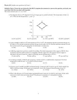
SCA2003-40: NEW REPRESENTATIVE SAMPLE
SELECTION CRITERIA FOR SPECIAL CORE ANALYSIS
Shameem Siddiqui, Taha M. Okasha, James J. Funk, Ahmad M. Al-Harbi
Saudi Aramco, Dhahran, KSA
This paper was prepared for presentation at the International Symposium of th e Society of Core
Analysts held in Pau, France, 21-24 September 2003
Abstract
To this date there is hardly any specific industry guideline for selecting representative samples for
special core analysis (SCAL) tests. No one can deny the importance of SCAL data in the
development of appropriate reservoir engineering models. This paper describes some of the
effective criteria and tests required for the selection of representative samples for use in SCAL
tests. The proposed technique is essential to insure that high quality core plugs are chosen to
represent appropriate flow compartments or facies within the reservoir. The absence of a
petrophysical input in the selection of SCAL plugs can result in SCAL data being NOT
representative of the reservoir or its flow compartments. Often, visual inspection and sometimes,
computerized tomography (CT) images are the only techniques used for assessing and selecting
native state core plugs for SCAL studies. Although it is possible to measure the effective brine
permeability (Kb ), there is no routine method for determining the porosity (φ) of the SCAL plugs
without compromising their wettability. Some of the existing selection criteria involve using the
conventional core analysis data (k and φ) on ‘sister plugs’ as a general indicator of the properties
of the SCAL samples. However, the uncertainties surrounding the extent of heterogeneity as
well as the exact depth of the plugs make it difficult to ascertain plugs as representative of a
particular flow compartment. The proposed technique identifies intervals with similar
porosity/permeability relationships. It uses a combination of wireline logs, gamma scan,
quantitative CT and preserved state brine permeability data to calculate appropriate depth-shifted
reservoir quality index (RQI) and flow zone indicator (FZI) data, which are then used to select
representative plug samples from each reservoir compartment.
Introduction
Coring is a very expensive operation. The main goal of coring is to retrieve core samples from
the well in order to get maximum amount of information about the reservoir. Core samples
collected provide very important petrophysical, petrographic, paleontological, sedimentological,
and diagenetic information. From a petrophysical point-of-view, the whole core and plug
samples typically undergo the following tests: CT-scan, gamma-scan, conventional tests, special
core analysis (SCAL) tests, rock mechanics and other special tests. The data are combined to get
information on heterogeneity; depth-shift between core and log data; whole core and plug
porosity and permeability; porosity-permeability relationship; fluid content (Dean Stark),
Reservoir Quality Index (RQI); Flow Zone Indicator (FZI), wettability, relative permeability,
capillary pressure, stress-strain relationship, compressibility, etc. The petrophysical data
generated this way play very important roles in reservoir characterization and modeling, log
calibration, reservoir simulation, and overall field production and development planning.
1
Among all the petrophysical tests, the SCAL tests which include wettability, capillary pressure,
relative permeability and capillary pressure determination are very important and timeconsuming. A reservoir condition relative permeability test can sometimes run for several
months when mimicking the actual flow mechanisms taking place in the field. So, it is very
important to design these tests properly and in particular to select the samples that ensure
meaningful results. In short, the samples must be ‘representative samples,’ which can capture the
overall variability within the reservoir in a more scientific way. Unfortunately, the most
important aspect of all SCAL procedures, the sample selection is one of the least talked about
subjects. According to Corbett et al. [2001], the API’s RP40 (Recommended Practices for Core
Analysis) makes very little reference to sampling and similarly, textbooks on Petrophysics do not
have sections on sampling. They [Corbett et al., 2001] made a good review of some of the
statistical, petrophysical and geological issues for sampling and proposed a series of
considerations. This has led to the development of a method using Hydraulic Units in a relatively
simple clastic reservoir [Mohammed and Corbett, 2002].
In this paper some issues related to sample selection criteria, with special focus on carbonate
reservoirs will be discussed. A large data set of conventional, whole core, and special core
analyses on a well in an Upper Jurassic carbonate reservoir was used to characterize
‘representative samples’ for special core analysis tests.
Reservoir Quality Index and Flow Zone Indicator
Core porosity and permeability measurements are extremely important for proper selection of
flow zones within a particular reservoir. Stiles [1949], Testerman [1962], and Nelson [1994] are
among researchers who worked extensively on porosity, permeability and reservoir zonation
issues using synergistic information that can be obtained from routine core analysis data and
elements of reservoir layering techniques.
The method proposed by Amaefule et al. [1993] is frequently used for characterizing flow zones
having similar hydraulic properties. The method uses a modified version of the Carman-Kozeny
equation and the mean hydraulic radius concept. The method is widely applied on scales from
the pore level through the inter-well level. Amaefule et al. [1993], defined three terms that are
convenient for use with conventional core analysis data. These are the reservoir quality index
(RQI), The normalized porosity (NPI), and the flow zone indicator (FZI). They are defined by:
RQI = 0.0314×
K …………...…………………………….……………..1
φ
φ ………………..……………………………….………….…2
NPI =
1 −φ
FZI =
RQI
………………………………………………………..……..3
NPI
Where,
RQI
K
φ
= Reservoir quality index (µm),
= Permeability (md), and
= Porosity (fraction).
2
According to Tiab and Donaldson [1996], samples with the same FZI values have similar pore
throat size, and thus constitute a flow unit. FZI is typically calculated using conventional core
analysis derived porosity and permeability data on the so-called ‘sister-plugs’ but that information
may not apply to the wettability-preserved actual SCAL plugs. Although it is not so difficult to
get the brine permeability data for a SCAL plug, it is almost impossible to determine its porosity
without compromising the wettablility state of the sample. CT provides a solution to this problem
by allowing the calculation of porosity values without taking the samples out of the brine.
CT-Scanning
Until the early 80’s special core analysis samples were chosen using visual inspection. The
introduction of Computerized Tomography (CT) in petrophysical analysis revolutionized the
sample selection process as it became possible to look at the ‘inside of the core plugs’ and to
select ‘good’ plugs before using them in long-duration SCAL tests, thus reducing rates of failure.
CT is a very powerful tool for detailed characterization and fluid flow visualization for evaluating
reservoir rocks in a non-destructive manner. During scanning, the X-ray source and detectors
move around the object to cover the entire 360 degrees at each scan location to make a ‘slice’ of
attenuation data. At high X-ray energies, the attenuation becomes mainly a function of the
electron density of the materials present in the object being scanned. CT number, the parameter
measured by all medical-based CT-scanners, is a relative scale of attenuation coefficients (uses
the value of -1000 for air and 0 for water). For a properly calibrated artifact-free system, the CT
number varies linearly with the bulk density of a rock [Vinegar and Wellington, 1987]. By using
appropriate brine and grain density data, very accurate porosity values can be obtained for every
slice of a wetta bility-preserved SCAL sample [Siddiqui, 2000].
Reservoir Zonation Using Cumulative RQI
The combination of φ and k data in terms of reservoir quality index (RQI) provides a convenient
starting point to address the differences between samples and between reservoir zones. If the
total productivity of a well is assumed to be a linear combination of individual flow zones, then a
simple summation and normalization of permeability, RQI, or FZI starting at the bottom of the
well provides a convenient comparison with the normalized cumulative plot of an open-hole flow
meter test. In such a plot consistent zones are characterized by straight lines with the slope of the
line indicating the overall reservoir quality within a particular depth interval. The lower the slope
the better the reservoir quality. In general these lines will coincide with Testerman’s [1962]
layers [Funk et al., 1999]. The equation used for calculating Normalized Cumulative RQI
(NCRQI), in this paper is as follows.
NCRQI
i Κi
∑
x =1 φ i
=
n Κi
∑
x =1 φ i
…………………………………………………... 4
where,
n = total number of data
i = number of data points at sequential steps of calculation
3
By plotting NCRQI versus depth it is possible to divide the reservoir into several zones by
observing changes in the slope. Consistent RQI zones are characterized by straight lines with
slope of the line indicating the overall reservoir quality within a particular depth interval. The
smaller the slope, the better the reservoir quality. Typically this type of zonation technique works
better in carbonate reservoirs where the typical RQI vs. NPI values [Amaefule et al., 1993] don’t
line up properly along parallel straight lines.
Heterogeneity Classification
In reservoir characterization heterogeneity specifically applies to the variability that affects flow
[Jensen et al., 1997]. One of the commonly used techniques for measuring the static
heterogeneities is the Lorenz (sometimes known as the Stile’s) Plot, which gives the Lorenz
Coefficient, Lc. The technique involves ordering the product of permeability and the
representative thickness (kh) in the descending order along with the corresponding porosityrepresentative thickness product (φh) for a well (or wells). The normalized cumulative values of
kh, which also known as the fraction of total flow capacity (between 0 and 1) are then plotted
against the normalized cumulative values of φh, which is also known as the fraction of the total
volume (between 0 and 1). The Lc is calculated by comparing the area under the curve above a
45° line between (0,0 and 1,1) and 0.5. Lc can theoretically vary between 0 and 1, with 1
representing the highest degree of heterogeneity. Details of the procedure for calculating Lc can
be found in the literature [Craig, 1971; Jensen et al., 1997].
The coefficient of variation, Cv is another measure of heterogeneity. It is a dimensionless
measure of sample variability or dispersion [Jensen et al., 1997], and is given by,
Cv =
Var( x )
…………………………………………......……..……. 5
E( x )
where, the numerator is the sample standard deviation and the denominator is the sample mean.
Cv is being increasingly applied in geological and engineering studies as an assessment of
permeability heterogeneity (Saner and Sahin, 1999). For data from different populations, the
mean and standard deviation often tend to change together such that Cv stays relatively constant.
Any large changes in Cv between two samples indicate a dramatic difference in the populations
associated with those samples [Jensen et al., 1997].
Results
For this study, a well from an Upper Jurassic carbonate reservoir was chosen on which extensive
log, and core data were available. The core tubes were gamma-scanned first, from which it was
found that the core depths needed to be shifted down by 6.5 ft for the entire cored length to match
with the log depths. Then the entire cored section was plugged thoroughly to collect about 375
SCAL plugs, which were kept preserved in brine, and about 180 other plugs, which were leached
and dried for conventional core analysis tests.
Brine permeability was run on most of the SCAL plugs under the wettability-preserved condition.
The 375 SCAL samples were then CT-scanned (full coverage, about 9 slices per plug) and the
raw data were transferred to a SUN workstation for generating statistical data (typically, mean,
standard deviation, minimum and maximum CT number) on circular regions-of-interest
4
representing the core materials. Then appropriate conversion equations were applied to obtain
porosity data for each slice of a plug and their average was recorded. The depth-shifted core data
were then compared with the logs, which showed a very good agreement between these two
independent sets of data (see Figure 1).
Using the CT-derived porosity and brine permeability data on the SCAL plugs, the RQI, NPI, FZI
and NCRQI values were calculated. Figure 2 shows the NCRQI values plotted as a function of
depth for the SCAL plugs as well as the more continuous conventional core analysis generated
NCRQI vs. depth data. By closely observing these two sets of data, a total of eight zones were
identified within the cored section, each with a different slope, as shown by the solid line
segments. For reference, the cumulative production data from a PLT test are also shown and it
shows trends similar to what was seen by Funk et al. [1999]. Figure 2 also shows demarcations
(dotted horizontal lines) based on original geological facies data.
The SCAL plugs were then subjected to screening based on various heterogeneity and related
criteria. Typically plugs with large inter-slice and intra-slice heterogeneities are eliminated from
SCAL tests. Figure 3 shows one example each of inter-slice and inter-slice heterogeneities. The
image on the left contains an anhydrite nodule in the last three slices, rendering it unsuitable for
SCAL tests. The image on the right shows a case of intra-slice heterogeneities where each slice
looks alike but there is a large variation of CT numbers within each slice. For eliminating the
plugs with inter-slice variations the ratio between the maximum and minimum CT numbers
within each plug was calculated and plugs having a ratio of 1.09 or more were discarded. For
eliminating the samples with intra-slice variations the plugs with average of the Cv of CT
numbers for each slice (standard deviation divided by mean) above 0.08 were eliminated as
heterogeneous. Additionally, plugs having a porosity of 5% or less were also eliminated and a
final list of 134 plugs was created that were suitable for SCAL studies.
Figure 4 is the classic RQI versus FZI plot [Amaefule et al., 1993] for the suitable plugs, which
are also classified according to the zone using different symbols. It also shows six diagonal lines,
each pair of which representing a range of FZI values. Upon close examination a total of five bin
sizes were chosen to group the core plugs into different FZI ranges. These are 0 to 1 inclusive, 1
to 2 inclusive, 2 to 3 inclusive, 3 to 4 inclusive, and greater than 4. Table 1 shows the SCAL
plugs listed according to these FZI bin sizes as well as the zones identified previously. In order to
make a representative composite core plug for say Zone 1, one can have several choices of FZI
ranges. Once an FZI range is selected, one composite plug for each zone should be sufficient for
conducting representative SCAL tests. It is also possible to mix plugs with different FZI values
but within the same zone in order to get an idea about the overall variations possible within the
zone. It may be noted that in this particular case Zones 6 and 8 have the steepest slope and they
contribute almost nothing to the production. Therefore testing samples from these two zones can
be avoided.
The use of the so-called sister plugs is common in making inferences about the behavior of the
plugs used for SCAL tests because of unavailability of some critical data such as porosity and
permeability. It was found that while porosity data didn’t vary so much for the short distance
(typically within one foot between the SCAL and the corresponding ‘sister’ conventional plug
sample), the permeability varied sometimes by one or two orders of magnitude. This is evident in
Figure 5, where the Lorenz plots are generated for the SCAL and conventional core analysis
plugs on which permeability data were available. Results showed a large difference between the
5
two Lorenz coefficient values, with the coefficient for the SCAL plugs having a value of 0.57
compared to the coefficient for conventional plugs having a value of 0.72. Although some of the
difference may be due to the sampling or experimental bias, one should be careful in using sister
plug data in serious calcula tions especially when permeabilities and overall heterogeneities are
concerned.
Conclusions
1. A set of guidelines has been established to select the ‘representative’ core plug samples
for special core analysis tests based on a combination of reservoir zonation, heterogeneity
analysis and application of RQI and FZI-based techniques.
2. This research finds CT-scanning to be an extremely useful tool for quantifying
heterogeneities within small plugs.
3. Samples picked up from a zone based on the normalized cumulative RQI based technique
demonstrated here have a better chance of representing that zone than samples picked up
at random from the entire cored section.
4. Using the properties of the sister plugs, especially for permeability and heterogeneity,
may lead to strange results.
Acknowledgments
The authors wish to thank Saudi Aramco to present and publish this paper. Special thanks also go
to their colleagues at the Petrophysics Unit of the Saudi Aramco Research and Development
Center in Dhahran, Saudi Arabia.
References
Amaefule, J. O., Altunbay, M., Tiab, D., Kersey, D. G., and Keelan, D. K: “Enhanced Reservoir
Description: Using core and log data to identify Hydraulic (Flow) Units and predict permeability
in uncored intervals/wells,” SPE 26436, presented at 68th Ann. Tech. Conf. and Exhibition,
Houston, TX, 1993.
Corbett, P. Potter, D., Mohammed, K., and Liu S.: “Forget Better Statistics - Concentrate on
Better Sample Selection,” Proceedings of the 6th Nordic Symposium of Petrophysics held in
Trondheim, Norway, May 15-16, 2001, 4 pp.
Craig Jr., F. F.: The Reservoir Engineering Aspects of Waterflooding, SPE of A.I.M.E., Dallas,
1971, pp. 64-66.
Jensen, J. L., Lake, L. L., Corbett, P. W. M. and Goggin, D. J.: Statistics for Petroleum Engineers
and Geoscientists, Prentice Hall, Upper Saddle River, New Jersey, 1997, pp. 144-166.
Mohammed, K. and Corbett, P.: “How Many Relative Permeability Measurements Do You
Need? A Case Study from a North African Reservoir,” SCA Paper No. 2002-03, Presented at the
2002SCA Symposium held in Monterey, California, September 23-26, 2002.
6
Nelson, P. H.: “Permeability-Porosity Relationships in Sedimentary Rocks,” The Log Analyst,
May-June, 1994, p. 38.
Funk J. J., Balobaid, Y. S., Al-Sardi, A. M. and Okasha, T. M.: Enhancement of Reservoir
Characteristics Modeling, Saudi Aramco Engineering Report No. 5684, Saudi Aramco, Dhahran,
November, 1999.
Saner, S., Sahin A.: “Lithological and Zonal Porosity-Permeability Distributions in the Arab-D
Reservoir, Uthmaniyah Field, Saudi Arabia,” AAPG Bull V 83, No 2, February 1999, pp 230243.
Siddiqui, S.: “Application of Computerized Tomography in Core Analysis at Saudi Aramco,”
Saudi Aramco Journal of Technology, Winter, 2000-2001, pp. 2-14.
Siddiqui, S., Funk, J., and Khamees A.: "Static and Dynamic Measurements of Reservoir
Heterogeneities in Carbonate Reservoirs," SCA paper No. 2000-06, presented at the 2000 SCA
Symposium held in Abu Dhabi, UAE, October 18 - 22, 2000
Stiles, W. E.: “Use of Permeability Distribution in Water Flood Calc ulations,” Petroleum
Transactions, A.I.M.E. (1949) 186, pp. 9-13.
Testerman, J. D.: “A Statistical Reservoir-Zonation Technique,” The Journal of Petroleum
Technology, (August, 1962), Trans., A.I.M.E. 225. pp. 889-893.
Tiab, D., and Donaldson, E. C., Petrophysics: Theory and practice of measuring reservoir rock
and fluid transport properties, Gulf Publishing, Houston, TX, 1996, 706 pp.
Vinegar, H. J. and Wellington, S. J.: “Tomographic Imaging of Three-Phase Flow Experiments,”
Rev. Sci. Instrum., 58 (1), January, 1987, p. 96-107.
7
6460
6480
6469
6475
6480
6500
6495
6500
6504
6520
Zone 1
Zone 2
6520
6540
6540
6560
6560
Zone 3
Zone 4
6562
6580
Depth (ft)
Depth (ft)
6580
6600
6620
Zone 5
6600
Zone 6
6620
6640
Zone 7
6647
6660
6640
Zone 8
6680
6660
6700
6680
6705
Norm. Cum. RQI (Conv plug)
6720
Norm. Cum. RQI (CT Plugs)
PHIT
6700
Geological Zone
6760
6720
0.00
Fraction of Cum. Production
6740
Avg. CT Porosity for Plug
0.05
0.10
0.15
0.20
0.25
0.30
0.35
0.0
0.40
Porosity (fraction)
0.1
0.2
0.3
0.4
0.5
0.6
0.7
0.8
0.9
1.0
Normalized RQI
Figure 2: Normalized Cumulative RQI vs. depth for the SCAL and conventional
core analysis plugs showing the existence of eight distinct zones within the cored
section (shown by solid line segments). The cumulative production data and the
geological zone markers (dotted horizontal lines) are also shown for reference.
Figure 1: CT-derived SCAL plug porosity data compared against the logs show a
very good agreement between the two independently derived sets of data.
8
10.00
RQI Zone 1
RQI Zone 2
RQI Zone 3
RQI Zone 4
RQI Zone 5
RQI Zone 6
RQI Zone 7
RQI Zone 8
FZI=4
1.00
FZI=3
FZI=2
FZI=1
FZI=0.5
RQI
FZI=0.1
0.10
Figure 3: CT-Scan slices showing case of inter-slice heterogeneity (left image), and
intra-slice heterogeneity (right image). The image on the left shows the presence of
a distinct anhydrite nodule in the last three slices, making it unsuitable for SCAL
tests. The image on the right shows large variations within each slice, with
relatively small channels available for flow and therefore unsuitable for SCAL tests.
0.01
0.010
0.100
1.000
NPI
Figure 4: RQI versus NPI plot for the small subset of plugs suitable for SCAL tests
after eliminating the heterogeneous or low-porosity plugs. The diagonal lines
correspond to six FZI values.
9
1.0
Lc (Conv-Plug) = 0.725
0.9
Lc (SCAL-Plug) = 0.566
Fraction of Total Flow Capacity
0.8
0.7
0.6
0.5
0.4
0.3
0.2
Fraction of Flow Cap (Routine Core)
Fraction of Flow Cap (CT-Plug)
0.1
0.0
0.0
0.1
0.2
0.3
0.4
0.5
0.6
0.7
0.8
0.9
1.0
Fraction of Total Flow Volume
Figure 5: Lorenz plots illustrating the difference between the sister plugs used for
SCAL and conventional core analysis tests.
10
Table 1: The final grouping of the SCAL plugs according to various FZI bin sizes and zones
FZI Range: 0 to 1
FZI Range: 1 to 2
FZI Range: 2 to 3
FZI Range: 3 to 4
FZI Range: >4
Plug Zo Avg.
kb
RQI FZI Plug Zo Avg. k b
RQI FZI Plug Zo Avg. k b
RQI FZI Plug Zo Avg.
kb
RQI FZI Plug Zo Avg. k b
RQI FZI
No. ne CT (md)
No. ne CT (md)
No. ne CT (md)
No. ne
CT (md)
No. ne CT (md)
Poro
Poro
Poro
Poro
Poro
1004 1 0.394
2.3 0.076 0.12 1016 1 0.313 75.5 0.488 1.07 1025 1 0.219 121.2 0.739 2.63 1037 2 0.258 309.4 1.087 3.13 1042 2 0.264 626.2 1.529 4.26
1006 1 0.424
3.8 0.095 0.13 1031 2 0.278 143.7 0.714 1.85 1029 1 0.252 218.4 0.925 2.75 1039 2 0.239 251.6 1.019 3.25 1147 4 0.216 281.5 1.134 4.12
1011 1 0.392 65.4 0.405 0.63 1032 2 0.280 164.1 0.760 1.96 1030 1 0.276 184.4 0.811 2.12 1071 4 0.231 273.9 1.081 3.60 1151 4 0.229 496.5 1.462 4.92
1012 1 0.306 22.6 0.270 0.61 1034 2 0.302 57.7 0.434 1.01 1033 2 0.269 153.4 0.750 2.04 1091 4 0.248 248.6 0.994 3.01 1152 4 0.221 425.1 1.377 4.85
1015 1 0.141
2.0 0.117 0.71 1041 2 0.284 143.8 0.707 1.79 1036 2 0.246 211.1 0.920 2.83 1098 4 0.229 200.1 0.927 3.12 1156 4 0.229 374.5 1.269 4.26
1023 1 0.164
4.2 0.159 0.81 1044 2 0.251 93.1 0.604 1.80 1040 2 0.271 196.0 0.845 2.28 1113 4 0.229 241.3 1.019 3.43 1165 4 0.225 646.0 1.682 5.78
1026 1 0.301
2.9 0.097 0.23 1053 3 0.306 102.3 0.574 1.30 1043 2 0.251 183.9 0.849 2.53 1117 4 0.230 215.7 0.961 3.21 1172 5 0.194 367.8 1.366 5.67
1027 1 0.258 14.4 0.234 0.67 1076 4 0.292 58.5 0.445 1.08 1047 3 0.262 235.6 0.942 2.65 1127 4 0.192 118.6 0.781 3.29 1270 7 0.181 623.0 1.840 8.30
1045 2 0.304 23.4 0.275 0.63 1079 4 0.296 74.8 0.499 1.19 1066 4 0.300 341.0 1.058 2.46 1132 4 0.217 184.2 0.915 3.30 1271 7 0.163 468.1 1.682 8.64
1046 3 0.294 26.7 0.299 0.72 1084 4 0.265 82.4 0.553 1.53 1067 4 0.265 269.0 1.001 2.78 1135 4 0.233 228.5 0.983 3.23 1272 7 0.169 715.1 2.044 10.07
1048 3 0.279 37.9 0.366 0.94 1085 4 0.254 105.5 0.640 1.88 1069 4 0.237 149.5 0.789 2.54 1136 4 0.229 276.7 1.093 3.69 1275 8 0.181 541.7 1.719 7.79
1049 3 0.306 12.2 0.198 0.45 1094 4 0.245 34.3 0.372 1.15 1072 4 0.279 229.0 0.900 2.33 1137 4 0.238 323.2 1.157 3.70 1286 8 0.149 120.1 0.891 5.07
1050 3 0.301 54.6 0.423 0.98 1115 4 0.253 110.9 0.657 1.94 1074 4 0.233 187.3 0.890 2.93 1139 4 0.230 222.9 0.978 3.28 1288 8 0.144 222.6 1.232 7.30
1051 3 0.305
2.6 0.092 0.21 1116 4 0.259 95.9 0.604 1.72 1083 4 0.272 276.6 1.000 2.67 1140 4 0.229 254.6 1.047 3.53
1052 3 0.303
4.2 0.117 0.27 1123 4 0.247 82.4 0.574 1.75 1086 4 0.279 173.2 0.783 2.03 1141 4 0.239 276.7 1.069 3.41
1054 3 0.299 35.5 0.342 0.80 1128 4 0.145 15.0 0.320 1.89 1087 4 0.264 196.0 0.855 2.38 1144 4 0.226 270.2 1.085 3.71
1055 3 0.276 18.3 0.256 0.67 1159 4 0.169
9.6 0.237 1.16 1088 4 0.271 245.4 0.946 2.55 1145 4 0.224 254.2 1.058 3.67
1059 3 0.256
1.7 0.081 0.23 1163 4 0.164 13.9 0.289 1.47 1089 4 0.258 190.4 0.853 2.45 1153 4 0.236 257.7 1.038 3.37
1062 4 0.277
2.1 0.087 0.23 1198 6 0.251 84.9 0.578 1.72 1090 4 0.242 200.0 0.902 2.82 1164 4 0.207 184.1 0.937 3.59
1063 4 0.284 10.1 0.188 0.47 1210 6 0.217 18.0 0.286 1.03 1093 4 0.228 175.1 0.870 2.94 1197 5 0.245 259.5 1.022 3.15
1064 4 0.232
1.4 0.076 0.25 1289 8 0.119
3.9 0.179 1.32 1095 4 0.235 123.9 0.720 2.34
1065 4 0.265
0.9 0.058 0.16 1318 8 0.105
1.9 0.135 1.14 1099 4 0.224 84.7 0.611 2.12
1080 4 0.286 40.8 0.375 0.94 1326 8 0.143
5.0 0.186 1.12 1100 4 0.223 83.9 0.609 2.12
1092 4 0.241
9.2 0.194 0.61 1331 8 0.127
7.7 0.246 1.69 1125 4 0.253 199.0 0.881 2.60
1096 4 0.253 12.8 0.223 0.66 1364 8 0.099
1.9 0.136 1.23 1138 4 0.233 190.0 0.897 2.95
1104 4 0.238
5.0 0.144 0.46
1146 4 0.232 164.3 0.835 2.76
1105 4 0.231
6.2 0.162 0.54
1155 4 0.246 208.4 0.914 2.80
1114 4 0.252
3.8 0.123 0.36
1199 6 0.245 179.3 0.850 2.62
1118 4 0.250 19.6 0.278 0.84
1317 8 0.096
9.5 0.312 2.95
Background Color Legend
1120 4 0.218
1.5 0.081 0.29
1323 8 0.159 44.0 0.523 2.76
1122 4 0.209
6.7 0.178 0.68
1324 8 0.148 26.4 0.419 2.41
Zone1
1133 4 0.233 14.8 0.250 0.82
1360 8 0.151 23.5 0.392 2.21
Zone2
1143 4 0.159
1.3 0.091 0.48
Zone3
1149 4 0.152
0.9 0.074 0.41
Zone4
1154 4 0.245 12.7 0.226 0.70
Zone5
1157 4 0.210
1.1 0.072 0.27
Zone6
1158 4 0.200
3.1 0.124 0.49
Zone7
1167 4 0.248
3.2 0.112 0.34
Zone8
1169 4 0.190
1.0 0.072 0.31
1171 5 0.170
3.7 0.146 0.71
1200 6 0.256
0.6 0.048 0.14
1204 6 0.264
1.2 0.066 0.18
1274 7 0.142
2.9 0.143 0.87
1290 8 0.113
1.2 0.104 0.81
11