CVTree3 User’s Manual
Guanghong ZUO and Bailin HAO
30 January 2014
Contents
1 Introduction
3
2 Web Server Structure
3
3 Web Interface
3.1 Getting Started . . . . . . . . . . . . . . . . . . . . .
3.2 Setting Up A Project . . . . . . . . . . . . . . . . . .
3.2.1 Basic Parameters . . . . . . . . . . . . . . . .
3.2.2 Choosing Inbuilt Genomes . . . . . . . . . . .
3.2.3 Upload Genomes . . . . . . . . . . . . . . . .
3.2.4 Run Project . . . . . . . . . . . . . . . . . . .
3.3 Result Page . . . . . . . . . . . . . . . . . . . . . . .
3.3.1 Monophyleticity, Collapsing, and Convergence
3.3.2 Summary of Taxa Monophyleticity with K . .
3.4 CVTree Viewer . . . . . . . . . . . . . . . . . . . . .
3.4.1 Use of Circles and Colors . . . . . . . . . . . .
3.4.2 Search Query . . . . . . . . . . . . . . . . . .
3.4.3 Select Node . . . . . . . . . . . . . . . . . . .
3.4.4 Output Tree Figure . . . . . . . . . . . . . . .
3.5 Taxonomy Revision and Recollapsing . . . . . . . . .
3.5.1 Taxonomic References . . . . . . . . . . . . .
3.5.2 Taxonomic Revision file . . . . . . . . . . . .
3.5.3 User Uploaded Genomes . . . . . . . . . . . .
3.6 Example Project . . . . . . . . . . . . . . . . . . . .
3.7 Keep and Reload a Project . . . . . . . . . . . . . . .
4 Source Code Availability
.
.
.
.
.
.
.
.
.
.
.
.
.
.
.
.
.
.
.
.
.
.
.
.
.
.
.
.
.
.
.
.
.
.
.
.
.
.
.
.
.
.
.
.
.
.
.
.
.
.
.
.
.
.
.
.
.
.
.
.
.
.
.
.
.
.
.
.
.
.
.
.
.
.
.
.
.
.
.
.
.
.
.
.
.
.
.
.
.
.
.
.
.
.
.
.
.
.
.
.
4
4
5
5
7
8
8
9
9
10
12
12
13
13
14
14
15
15
16
17
18
18
1
5 Development History and
Acknowledgements
18
Appendices
20
A Inbuilt Genome Data Sets
A.1 Prokaryote Genomes . .
A.2 Fungi Genomes . . . . .
A.3 Eukaryote Genomes . . .
A.4 Tiny Genomes . . . . . .
.
.
.
.
20
20
20
21
21
.
.
.
.
21
21
22
22
24
.
.
.
.
.
.
.
.
.
.
.
.
.
.
.
.
.
.
.
.
.
.
.
.
.
.
.
.
.
.
.
.
.
.
.
.
.
.
.
.
.
.
.
.
.
.
.
.
.
.
.
.
.
.
.
.
.
.
.
.
.
.
.
.
B Algorithm
B.1 Frequency or Probability of Appearance of K-Strings
B.2 Subtraction of Random Background . . . . . . . . . .
B.3 Composition Vectors and Dissimilarity Matrix . . . .
B.4 Tree Construction . . . . . . . . . . . . . . . . . . . .
References
.
.
.
.
.
.
.
.
.
.
.
.
.
.
.
.
.
.
.
.
.
.
.
.
.
.
.
.
.
.
.
.
24
2
1
Introduction
CVTree3 is an effective tool for inferring phylogeny from whole genome
sequences and comparing the result with taxonomy. The alignment-free
method based on K-tuple counting and background subtraction was termed
composition vector (CV) approach. It was introduced in 2004 [Qi et al.
(2004b)] with applications to prokaryote phylogeny. The first web server was
published in the same year in the NAR Web Server issue [Qi et al. (2004a)].
Since then it has been applied to Archaea and Bacteria [Gao et al. (2007);
Qi et al. (2004b); Sun et al. (2010)], viruses [Gao and Qi (2007); Gao et al.
(2003)], chloroplasts [Yu et al. (2005)] and fungi [Choi et al. (2013); O’Connell
et al. (2012); Wang et al. (2009)]. An essential update of the CVTree web
server was published in the 2009 NAR Web Server issue [Xu and Hao (2009)].
As the CV algorithm is CPU and memory demanding, the previous
CVTree web servers could hardly catch up with the ever increasing amount
of genomic data. Therefore, we have redesigned the data processing strategy
and made the core program parallel. The new CVTree3 pipeline resides in a
dedicated cluster with 64 cores. An interactive, collapsible and expandable,
CVTree Viewer based on HTML5 has been added to the new web server.
These new features enable biologists to study phylogeny inferred from thousands of genomes and to compare the result directly with taxonomy at all
taxonomic ranks.
CVTree3 is accessed without login requirement in most browsers, e.g., IE,
FireFox, or google Chrome. However, the use of HTML5 makes IE browser
lower than IE 9.0 not fully supported.
Please cite CVTree as:
1. Qi J, Wang B, Hao BL (2004) Whole proteome prokaryote phylogeny
without sequence alignment, J. Mol. Evol. 58(1): 1 – 11.
2. Zuo GH, Hao BL (2014) CVTree3: An effective genome-based and
alignment-free phylogenetic tool with interactive tree display and taxonomic comparison, Nucl. Acids Res. Web Server issue, (submitted).
2
Web Server Structure
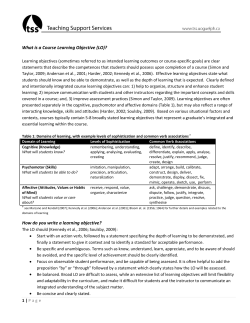
The structure of the CVTree3 web server is given schematically in Figure
1. The blocks with green background are visible and accessible to the user.
These will be explained in more details in the subsequent sections. The rest
of Figure 1 consists of three parts: monthly updating of the built-in dataset,
processing of user-uploaded data, and the project central. The blocks within
3
a dashed frame make the core of the CV algorithm, which has been parallelized in CVTree3. Arrows in the figure indicate the direction of execution.
Dashed-lines indicate optional operations.
The web server blocks serviceable to the user are described one by one in
what follows.
Figure 1: The structure of the CVTree3 web server
3
3.1
Web Interface
Getting Started
The Start Page of CVTree3 is shown in Figure 2. If a project has already been
created, it can be reloaded by entering the Project Number in the textbox
and clicking the “Load/Create Project’ button. To create a new project, just
leave the textbox blank and click “Load/Create Project”.
4
Figure 2: The Start Page of CVTree3
3.2
Setting Up A Project
After Load/Create a project, a Setup Page (see Figure 3) in “Setting parameters” status is opened. A unique Project Number shows up at the top of
the page. Please remember the Project Number for subsequent reloading.
The Setup Page starts with a Project Status bar which may indicate one of
three states: “Setting parameters”, “Running · · · ”, and “Project completed”
(see Figure 4).
The main body of the Setup Page consists of three titled fields, namely,
“Basic Parameters”, “Select Inbuilt Genomes”, and “Upload User’s Genomes”.
3.2.1
Basic Parameters
Basic Parameters are set by the user in the first field “Basic Parameters” of
the Setup Page.
Sequence Type: Though Protein sequences are preferred, DNA sequences
may be used as well.
K-tuple length: CVTree3 is capable to generate trees for all choosen K5
Figure 3: The Setup Page of CVTree3
Figure 4: The status of a project
tuple lengths in one run. The default Ks are from 3 to 7 for proteins and 6
to 18 with increment 3 for DNAs, though any single K value may be picked
up. We note that when protein sequences are used the best K range is 4 and
5 for viruses, 5 and 6 for prokaryotes, 6 and 7 for fungi [Li et al. (2010)]. The
K-values 8 and 9 are avaiable but usually not necessary.
An essentially new feature of the CVTree3 web server consists in allowing
the user to compare the tree branchings with taxonomy and to see the effect
of trial taxonomic revisions. For the Inbuilt Genomes the initial lineage
information is downloaded from the NCBI taxonomy and a default taxonomy
6
revision file is provided to modify a few apparently incorrect or incomplete
lineages. If a user would not like to invoke these revisions and a comparison
report would solely be based on the initial NCBI taxonomy, the Revised
Taxonomy box should be unchecked. For more about taxonomic revisions
please see Section 3.5.
Optionally, a user may enter an email and be notified when the project is
completed. Otherwise, the result may be reloaded at a later time using the
Project Number explained above.
3.2.2
Choosing Inbuilt Genomes
The CVTree3 web server possesses a comprehensive built-in database of
genomes. These genomes are subdivided into several groups as reflected
by the names of the selectable buttons: Archaea(165), Bacteria(2587), Tiny
Genomes(26), Fungi(83), and Eukarya(4), numerals in parentheses indicating the number of genomes in each group as of 1 January 2014. For more
about these genome groups, please see the Appendix A.
By clicking the checkbox in front of each group, one can select or unselect
a whole group. The outgroup will be chosen by the web server “at random”.
If one wants to select genomes one by one and set an outgroup by oneself, please get into the Select Inbuilt Genomes Page, shown in Figure 5, by
clicking on the “See Details” button.
This page consists of a long list of all builtin genomes. Entries in this
table is sortable by clicking on the head of the table. For example, by clicking
on “Genome name” all the genomes would appear in alphabetic order of their
names; by clicking on “Proteome” the genomes will be ordered by the total
number of amino acids in fraction of M (106 ) (this is so even when Sequence
type on the previous page was chosen to be DNA (FFN) ), just giving an
idea about the genome size.
The first column ”Out-group” is a toggle switch. Only one entry may be
selected while all others be unselected.
The last column of the table possesses a pull-down list of taxonomic ranks
with number of taxa in each rank: from Domian{3} to Species{1581} for the
time of writing these lines. A user can pick up an item from the list to
facilitate the selection of genomes.
After completing the selection one returns to the Project Set page (Figure 3) by clicking on “Done & Back to Project page”.
7
Figure 5: Select Inbuilt Genomes Page
3.2.3
Upload Genomes
In the functional field “Upload Genomes” a user can upload one’s own
genomes (see Figure 6). A list of all uploaded genomes appears in the
field, but only checked ones are used when the project is submitted for running. Note that all genomes are selected by default when uploaded. All user
genomes, checked or unchecked, together with the configured project will be
kept for 7 days after the last run.
User genomes may be uploaded as one or more compressed files (no more
than 100MB in total). They can be uploaded one by one or as a group.
Figure 6: Upload Genomes
3.2.4
Run Project
When all paramenters are set the project is submitted for processing by clicking the button “All parameters are fine, Run Project”. After submission the
8
“Setting parameters” status will be locked and the project status changes to
that shown in the middle of Figure 4, namely, “Running · · · ”. The project
will be done in a few minutes if only the inbuilt genomes are used. If many
new genomes are uploaded, the waiting time might be much longer, depending on the size and number of genomes. One can safely close the page and
the completion of job be notified later by email if an email has been entered
when setting parameters. Otherwise, one may revisit the web server and
reload the project by entering the Project Number.
If necessary one can cancel the project and reset parameters by clicking
the button “Cancel Project”.
3.3
Result Page
When the project is completed, the Project Status bar changes to that shown
in the bottom of Figure 4. By clicking on the “See Result” button one is led
to the Result Page.
The Result Page almost entirely consists of a long table summarizing taxa
convergence except for two buttons in the upper-right corner: “See Tree” and
“Download Result”.
“See Tree” is the portal to the interactive tree display to be described in
Section 3.4.
“Download Result” is where the user can download the results to the
local computer for further analysis and archiving. It may be used any time
while on-line or after reloading a project.
3.3.1
Monophyleticity, Collapsing, and Convergence
A prominent feature of the CVTree approach consists in that the resulted
trees are justified by direct comparison with taxonomy rather than by statistical resampling tests such as bootstrap or jackknife. Statistical resampling
tests tell at most the stability and self-consistency of the tree with respect
to small variations of the input data, by far not the objective correctness of
the trees. We note, nevertheless, the CVTree results have also successfully
passed various statistical resampling tests [Zuo et al. (2010)].
A central notion in comparing a tree with taxonomy is monophyleticity.
The notion of monophyleticity applies to phylogeny as well as to taxonomy,
see, e.g., discussion by James Farris [Farris (1974, 1990)]. However, we use
it in a pragmatic way by restricting to the classification of genomes in the
input dataset and to the collection of genomes in various tree branches.
If all genomes in a certain tree branch come from one and the same
taxon and no genomes from other taxa having mixed in, the branch is said
9
to be monophyletic at this taxonomic rank. For example, this happens to
Cyanobacteria as all the 74 genomes designated to this phylum in the input
dataset appear entirely and exclusively in one and the same branch. Now the
branch may be fully collapsed into one leave labeled by Cyanobacteria{74}.
In this way, the total number of leaves seen in a tree may be greatly reduced.
From a taxonomic point of view a taxon is monophyletic only when all
species listed in it are descendants of one and the same ancester. As this
is a hardly provable fact, monphyleticity has to be deduced from some phylogenetis study. For example, according to vol. 3 of The Bergey’s Manual,
77 species out from 167 listed in the genus Clostridium form a cluster in a
16S rRNA gene tree. These are considered members of Costridium senso
stricto, whereas the remaining 90 species are distributed in 10 different clusters. Naturally, one cannot expect a monophyletic branch of Clostridium
genomes for the time being. In CVTrees, there is a branch made of 31 out
from 43 genomes designated to Clostridium in the input data. This branch
may only be collapsed to Clostridium{31/41}.
When a branch is collapsed monophyletically to a leave made of genomes
from one and the same taxon, it is said to be convergent at this taxonomic
rank. In other words, only when collapsing leads to a monophyletic leave, the
taxon is considered convergent at the corresponding K. Usually this happens
at one or more K-values. Convergence at most or all K-values adds confidence
to the result, although the branching topology may be slightly different.
3.3.2
Summary of Taxa Monophyleticity with K
Convergence of taxa at various K-values provides an additional angle to look
at the phylogeny. That is why CVTree3 calculates trees at several Ks in one
run and produces a summary automatically.
The taxa convergence summary may be displayed in three ways: “Total”,
“Monophyly”, and “None”.
The “Total” way generates an alphabetic list of all taxa in taxonomic
order. Abbreviations are used for the ranks: ⟨P⟩ Phylum, ⟨C⟩ Class, ⟨O⟩
Order, ⟨F⟩ Family, ⟨G⟩ Genus, and ⟨S⟩ Species. The same set of abbreviations
with an additional ⟨T⟩ for sTrains are used in the CVTree Viewer.
A typical page is shown in the top part of Figure 7. A taxon name is
followed by the number of genomes belonging to the taxon. One can choose to
show the list from Domain down to a certain taxonomic rank, e.g., Family, by
setting “Show Taxonomy to Family”. The monophyly status of the taxon is
given at the right. For example, the archaeal class Halobacteria is represented
by 27 genomes and it is monophyletic at all K’s except for K = 4, then the
corresponding line in the list reads:
10
⟨C⟩ Halobacteria: 27
K3- -K5K6K7
Figure 7: The Taxa Convergence Summary
The option “Monophyly” lists taxa which are monophyletic at least for
one K, as shown in the middle of Figure 7. If one would like to see a list of
taxa which are not monophyletic for all K, the option “None” serves for this
purpose, see the lowest part of Figure 7.
When “Monophyly” is chosen, each taxonomic rank as a subtitle carries
a statistic. For example, a line
Class (24 + 45 /79)
tells that the totall number of classes is 79 in the input dataset (after taking
into account taxonomic revision, if any); among these 79 classes 24 are represented by only one genome hence are trivially monophyletic; the other 45
are represented by two or more genomes and are monophyletic at least for
one K.
11
In the “None” option, the corresponding line reads
Class (10/79)
indicating that there are 79−24−45 = 10 classes, which are not monophyletic
for whatsoever K. In a sense, these non-monophyletic taxa are worth further
studying as they may hint on possible txonomic revisions.
3.4
CVTree Viewer
It is extremely difficult, if not impossible, to comprehend a tree made of
thousands of leaves. To this end an interactive, collapsible and expandable,
display has been developed for the CVTree3 web server. As skillful manipulation of the display is the key point to make the most of CVTree3. Therefore,
we explain the interactive display in more details.
By clicking the button “See Tree” in the upper-right corner of the Result
Page (see Figure 7), a CVTree Viewer page with default K = 6 opens up. A
typical tree, plotted by using HTML5, is shown in Figure 8.
Figure 8: A typical page of CVTree Viewer
3.4.1
Use of Circles and Colors
If a node is denoted by a blank circle (◦), it is collapsible. One may click
on the circle to have all the lower branchings shrinked; the collapsed branch
is labeled by the highest-rank common taxon name. At the lowest level, a
12
rightmost node may be marked by a solid circle (•) preceding a taxon name;
it tells that there are more than one genomes in that branch and it may be
expanded by clicking on the solid circle. In contrast, a short line (—) in place
of a would-be circle means that there is only one genome and it cannot be
further expanded.
Taxon names may appear in one of three basic colors: red, blue, and
green. A red name indicates that the branch is monophyletic and collapsed.
This includes the case when a taxon is represented by a single genome, i.e.,
the taxon is trivially monophyletic.
A collapsed but not convergent branch such as Clostridium{31/43} is
shown in blue. A taxon name in green matches the word in “Search Query”
(see below).
3.4.2
Search Query
For the best K value 5 or 6 the CVtree Viewer first opens in a maximally
collaped state with 3 leaves: •⟨D⟩Bacteria⟨K⟩Bacteria{2587}, •⟨D⟩Archaea
⟨K⟩Archaea{165}, and •⟨D⟩Eukaryota{7}, representing the three main domains of life and witnessing the correctness of Carl Woese.
The quickest way to get to the point of interest in a tree is typing a taxon
name in place of the “Search Query”. For example, one may type Helicobacter and select an item from the pull-down list. Then Helicobacter{63} will
be highlighted in green with all the other branches maximally collapsed.
One can cut a branch and let it fills up the whole display window.
For example, to single out the branch Helicobacter{63} one holds the shift
key and clicks on the solid circle in front of the genus name. The leave
•Helicobacter{63} will move to the leftmost position in the display and further clicking on the solid circle expands it to the whole window.
3.4.3
Select Node
The aforementioned operation of cutting a branch may be performed in another way, namely, by using the “Select Node” option in the top line of
the CVTree Viewer. By selecting a taxon name in the pull-down list, e.g.,
⟨P⟩Aquificae{12}, the phylum Aquificae represented by 12 genomes for the
time being is displayed in the whole window. By selecting an higher taxon,
e.g., ⟨D⟩Bacteria{2587} the display restores to that for the whole domain
Bacteria.
13
3.4.4
Output Tree Figure
When a tree view has been adjusted by appropriately collapsing and expanding, a print quality figure can be obtained by clicking on the “output” button
in the upper-right corner of the CVTree Viewer page (Figure 8). It opens an
output preview page (Figure 9).
One may select a format to save a figure. The default format is SVG
(Scalable Vector Graphics), as the underlying plot is done in SVG. Before
saving, a figure may be monochromatized. One may choose PDF, eps, and
png formats as well. If a user wishes to modify the output figure, say, by
adding texts or changing color, the SVG format is recommended, especially,
when convenient SVG tools such as Inkscape is avalable.
Figure 9: The Output Preview Page of CVTree3
Please do not forget to quit the preview page in order to continue working
with the CVTree Viewer.
3.5
Taxonomy Revision and Recollapsing
Now we return to the prominent feature of CVTree approach, namely, justification of the resulted trees by direct comparison with taxonomy. For
prokaryotes this kind of comparison has become feasible only quite recently.
On one hand, the completion of the second edition of The Bergey’s Manual
of Systematic Bacteriology [Bergey’s Manual Trust (2012)], which has been
considered by many microbiologists as the best approximation to an official
14
classification [Konstntinidis and Tiedje (2005)], provides a state-of-the-art
framework for taxonomy together with current literature such as as International Journal of Systematic and Evolutionary Microbiology. On the other
hand, the development of the CVTree approach has provided prokaryotic
phylogeny a convenient and comprehensible platform [Hao (2011); Li et al.
(2010)].
3.5.1
Taxonomic References
Speaking about taxonomy one must admit that there is no generally accepted
standard for prokaryotic taxonomy. The temptation to become a standard
makes the Bergey’s systematics a more conservative source. There were
deadlines and other restrictions for inclusion in The Manual. Many newly
sequenced genomes do not have neither a standing in bacterial nomenclature
nor a validly published name. These organisms are not reflected in Bergey’s
Manual or in current literature. In contrast, the NCBI taxonomy, though
disclaimed to be a taxonomic reference, is, in fact, more dynamic and up-todate. At least, for any sequence deposited into GenBank there is a piece of
taxonomic information, no matter how imcomplete it might be.
3.5.2
Taxonomic Revision file
Therefore, the NCBI Taxonomy serves as an initial source for taxonomic information. In order to see this initial lineage information one should uncheck
the Revised taxonomy box in the Setup Page (Figure 3) during parameter
setting. Then in the Convergence of Taxa table in the Result Page one might
see a line
⟨P⟩Archaea:1
K3K4K5K6K7
among other lines. It is a bit strange as Archaea represents a ⟨D⟩, not a ⟨P⟩.
By entering ⟨P⟩Archaea into “Search Query” one sees that this comes from
halophilic archaeon DL31 uid72619{1}
Clearly, this was an organism without a validly published name. By moving the cursor to this name, a pull-down window with lineage information
appears for a few seconds. Indeed, it shows a lineage without proper assignment from ⟨P⟩ to ⟨F⟩ (the genus name “halophilic” was assigned during the
pre-processing of the NCBI taxonomic information, see the upper-left block
of Figure 1)
⟨D⟩Archaea⟨K⟩Archaea⟨P⟩Archaea⟨C⟩ Archaea⟨O⟩Archaea⟨F⟩Archaea⟨G⟩halophilic· · ·
However, the position of this genome in the tree clearly shows that it
belongs to the family Halobacteriaceae. One would like to see the effect of
15
making appropriate taxonomic revisions. The option “Taxonomy Revision”
in the CVTree Viewer provides this function. By clicking on this option an
empty “Taxonomy Revision” window opens up: it looks like Figure 10 but
without any content.
At this point one may see the effect of suggesting a revision. We use the
syntax of the UNIX/LINUX stream editor command “sed -f commandfile”,
i.e., by writing a line in the “commandfile”:
s/⟨P⟩Archaea· · · ⟨F⟩Archaea⟨G⟩halophilic/
⟨P⟩Euryachaeota⟨C⟩Halobacteria⟨O⟩Halobacteriales⟨F⟩Halobacteriaceae⟨G⟩halophilic/g
When the Taxonomy Revision file is ready, one clicks on the “Submit”
button in the bottom line. The system shows “Recollapsing is running.
Please wait.“ It takes a minute or two. Then it says “Recollapse successfully”.
Both the “Summary of taxa monophyleticity versus K” and the CVTree
Viewer have been renewed. One sees, e.g., a former line
⟨C⟩Halobacteria:26
-----------becomes
⟨C⟩Halobacteria:27
K3- -K4K5K6K7
and in the CVTrees the whole Halobacteria branch can be collapsed at all K
except for K=4.
As there are many explicit taxonomic problems in the initial NCBI information, we have prepared a default Taxonomic Revision file. If the Revised
taxonomy box is checked in the beginning the default file will be used for
comaprison with taxonomy; otherwise, the initial NCBI information is used.
Alternatively, one may use the buttons “Clear Text”, “Reset”, “Default”,
“Save”, and “Submit”, to manage the revision process. For example, “Clear
Text” makes the Taxonomy Revision file empty and “Default” restores it to
the default file. An user-generated Taxonomy Revision file, saved to the local
computer, may be used in subsequent new projects.
We emphasize that actual taxonomic revisions must comply with the
International Code of Nomenclature of Bacteria [Lapage et al. (1992)] and
follow the established practice in the microbiological community. The Taxonomy Revision function provided by CVTree3 is solely for trial purpose.
3.5.3
User Uploaded Genomes
No taxonomic information is required when uploading user supplied genomes,
because one would like to use CVTree3 to predict taxonomic position of
newly sequenced genomes. In the CVTree Viewer if the cursor is put on such
a genome, the lineage information would look like
16
Figure 10: A Taxonomy Revision file
⟨D⟩Todefine⟨K⟩Todefine⟨P⟩Todefine⟨C⟩Todefine ⟨O⟩Todefine⟨F⟩Todefine⟨G⟩Todefine· · ·
(A non-standard word “Todefine” is chosen instead of, say, “Undefined”,
to avoid possible confusion in background parsing.) Such genomes are not
counted in checking monopyleticity and generating convergence statistics.
However, known pieces of taxonomic information may be included in user’s
Taxonomy Revision file. For example, the four uploaded genomes shown in
Figure 6 are taken from the “microbial dark matter” [Rinke et al. (2013)]. By
inspecting the CVTree one can infer some taxonomic knowledge and insert
the following lines into the Taxonomy Revision file:
s/⟨D⟩Todefine⟨K⟩Todefine⟨P⟩Todefine∠C⟩Todefine⟨O⟩Todefine⟨F⟩Todefine⟨G⟩Todefine⟨S⟩/
⟨D⟩Archaea⟨K⟩Archaea⟨P⟩Euryarchaeota⟨O⟩Todefine⟨F⟩Todefine⟨G⟩Todefine⟨S⟩/g
3.6
Example Project
One can easily generate an example project by clicking “Load/Create Project”
button in the Start Page (see Figure 2), and then run the project by clicking
the button “Run Project” without changing any parameters in the Setup
17
Page (see Figure 3). The project will complete in a few minute, and the
status bar changes from what shown in the middle of Figure 4 to that in the
bottom of Figure 4. The result is ready for viewing by clicking the button
“See Result”.
3.7
Keep and Reload a Project
The unique Project Number assigned at setting up a new project is used for
reloading the project at a later time. After reloading one may adjust the
parameters and rerun the job. A project is kept for 7 days after the last run.
What kept includes
1. The parameter setting.
2. The user uploaded genomes.
3. The Taxonomic Revision file, usually produced by modifying the default file.
4
Source Code Availability
For academic users who are interested in the inner workings of the CVTree
algorithm we can provide a stand-alone CVTree program. It is capable to
calculate CVs and dissimilarity between CV pairs in comand window mode.
It does not contain web interface, automatic updating machinery, and parallelization. To get a free copy of the source code with a manual please write
to Dr. Guanghong Zuo at [email protected] with your full name and
affiliation indicated.
5
Development History and
Acknowledgements
The CV approach was first announced in 2002 at C. N. Yang’s 80th Birthday Conference [Hao et al. (2003)] and applied to coronovivuses [Gao et al.
(2003)] and prokaryotes [Qi et al. (2004b)]. Stand-alone CVTree programs
were written from scratch by Ji Qi, Lei Gao, Jiandong Sun, and Zhao Xu
independently at different times. The first CVTree web server was built by
Ji Qi and Hong Luo in 2004 [Qi et al. (2004a)]. An essentially improved update was constructed by Zhao Xu in 2009 [Xu and Hao (2009)]. The present
parallelized CVTree3 has been implemented by Guanghong Zuo since 2012
and tested by many colleagues.
18
The CVTree project has been supported by National Basic Research
Project of China (973 Programs No. 2007CB814800 and No. 2013CB834100),
and by the State Key Laboratory of Applied Surface Physics and Department
of Physics, Fudan University.
19
Appendices
A
Inbuilt Genome Data Sets
The Inbuilt Genome dataset consists of two major parts, a monthly updated
prokaryote genome set from NCBI [NCBI Resource Coordinators (2013)], and
a manually collected fungi genome set from FGI (Fungal Genome Initiative),
JGI (DOE Joint Genome Institute ), RFCG and other sources. As of 1
January 2014 there are in total 2865 organisms, including 2613 Bacteria, 165
Archaea, 83 Fungi and 4 non-fungal Eukaryotes.
User can either study phylogenetic relationship among Inbuilt Genomes or
upload their own data to the CVTree3 web server to be studied separately or
together with selected genomes from the inbuilt dataset. User can download
the inbuilt genomes from this web server but it is time consuming.
A.1
Prokaryote Genomes
There are two available sets of prokaryote complete genomes. Those in GenBank [Benson et al. (2013)] are the original data submitted by their authors.
Those at the National Center for Biotechnological Information (NCBI) are
reference genomes curated by NCBI staff. Since the latter represents the approach of one and the same group using the same set of tools, it may provide
a more consistent background for comparison. Therefore, we used all the
translated amino acid sequences (the .faa files with NC accession numbers)
from NCBI. This part of data is updated monthly.
A.2
Fungi Genomes
Fungal genomes are provided from the past and for the future. Historically,
82 genomes were listed because CVTree was applied to construct a fungal
phylogeny based on 82 genomes [Wang et al. (2009)]. Since then we have
updated some of these genomes, incidentally keeping the same total number.
The fungal genomes are provided mostly for the future as there is great
potential of applying CVTree to study their phylogeny. As nomenclature
and classification of fungi have not reached a state comparable with that of
prokaryotes, the extension and updating of fungal genomes will be carried
out only occasionally with a brief announcement on the fist page of the web
server.
20
A.3
Eukaryote Genomes
Currently we only provide 4 non-fungal Eukaryote genomes. They are Caenorhabditis elegans, Arabidopsis thaliana, Plasmodium falciparum and Drosophila
melanogaster. These genomes as used as outgroup in our prvious phylogenetic studies, e.g., [Gao et al. (2007)].
At present time thousands of eukaryotic genome sequencing projects are
under way. Accordingly we expect to enlarge the collection of eukaryote
genomes in anticipation of more phylogenetic studies using CVTree in the
future.
A.4
Tiny Genomes
There are a few highly degenerated genomes of bacterial endosymbiont bacteria in the inbuilt database. Their proteomes are very small (< 10000 amino
acids), hence the adjective “Tiny”. Due to lacking of many genes the position of these species in the phylogeny often turns out to be questionable,
e.g., they tend to the root and occasionally violate the trifurcation of the
three main domains of life. This is why we suggest not to include the “Tiny
Genomes” in a study of mostly “free-living” organisms.
On the other hand, if one is interested in these highly degenerated genomes,
then it should be reminded that the cut-off at 104 amino acids is artificial
and many slightly larger genomes, i.e., those from some insect symbionts in
the family Enterobacteriaceae must be taken into account as well.
B
Algorithm
Since the CVTree method has been described many times in the literature
[Hao (2011); Li et al. (2010); Qi et al. (2004b)], here we only present a brief
overview.
B.1
Frequency or Probability of Appearance of K-Strings
The alignment-free way of genome comparison is realized by extending single
nucleotide or single amino acid counting to that of longer K-strings. Among
early work along this line we mention the use of dinulceotide relative abundance as a genomic signature [Karlin and Burge (1995)]. Given a DNA or
amino acid sequence of length L, we count the number of appearance of
(overlapping) strings of a fixed length K in the sequence. The counting may
be performed for a complete genome or for a collection of translated amino
21
acid sequences. There are in total N possible types of such strings: N = 4K
for DNA and N = 20K for amino acid sequences.
For concreteness consider the case of one protein sequence of length L.
Denote the frequency of appearance of the K-String a1 a2 · · · aK by f (a1 a2 · · · aK ),
where each ai is one of the 20 amino acid single-letter symbols. This frequency divided by the total number (L − K + 1) of K-Strings in the given
protein sequence may be taken as the probability p(a1 a2 · · · aK ) of appearance
of the string a1 a2 · · · aK in the protein:
p(a1 a2 · · · aK ) =
f (a1 a2 · · · aK )
(L − K + 1)
(1)
The collection of such frequencies or probabilities reflects both the result of
random mutations and selective evolution in terms of K-strings as building
blocks.
B.2
Subtraction of Random Background
Mutations happen in a more or less random manner at the molecular level,
while selections shape the direction of evolution. Neutral mutations lead
to some randomness in the K-string composition. In order to highlight the
selective diversification of sequence composition one must subtract a random
background from the simple counting results. This is done as follows.
Suppose we have done direct counting for all strings of length (K −1) and
(K − 2). The probability of appearance of K-strings is predicted by using a
Markov model:
p(a1 a2 · · · aK−1 )p(a2 a3 · · · aK )
p0 (a1 a2 · · · aK ) =
(2)
p(a2 a3 · · · aK−1 )
The superscript 0 on p0 indicates the fact that it is a predicted quantity. We
note that the denominator comes from the frequency of (K − 2)-strings. This
kind of Markov model prediction has been used in biological sequence analysis
since long [Brendel et al. (1986)]. It can be justified by virtue of a maximal
entropy principle with appropriate constraints [Hu and Wang (2001)].
B.3
Composition Vectors and Dissimilarity Matrix
It is the difference between the actual counting result p and the predicted
value p0 that really reflects the shaping role of selective evolution. Therefore,
we collect
{
p(a1 a2 ···aK )−p0 (a1 a2 ···aK )
when p0 ̸= 0
p0 (a1 a2 ···aK )
ai (a1 a2 · · · aK ) =
(3)
0
when p0 = 0
22
for all possible strings a1 a2 · · · aK as components to form a composition vector
for a species. To further simplify the notations, we write ai for the i-th
component corresponding to the string type i, where i runs from 1 to N =
20K . Putting these components in a fixed order, we obtain a composition
vector for the species A:
A = (a1 , a2 , · · · , aN )
Likewise, for the species B we have a composition vector
B = (b1 , b2 , · · · , bN )
In principle there are different ways to construct the composition vectors.
First, one may use the whole genome sequence. Second, one may just collect
the coding sequences in the genome. Third, one makes use of the translated
amino acid sequences from the coding segments of DNA. As mutation rates
are higher and more variable in non-coding segments and protein sequences
change at a more or less constant rate, one expects that the third choice is
the best and the second is better than the first. We tried all three choices and
the requirement of consistency served as a criterion. By consistency we mean
the topology of the trees constructed with growing K should converge. This
is best realized with phylogenetic relations obtained from protein sequences.
Therefore, in what follows we concentrate on results based on amino acid
sequences.
The correlation C(A, B) between any two species A and B is calculated
as the cosine function of the angle between the two representative vectors in
the N -dimensional space of composition vectors:
∑N
a i × bi
C(A, B) = ∑N i=1 ∑N
(4)
1
2
( i=1 ai × i=1 b2i ) 2
The distance D(A, B) between the two species is defined as
D(A, B) =
1 − C(A, B)
2
(5)
Since C(A, B) may vary between -1 and 1, the distance is normalized to the
interval (0, 1). The collection of distances for all species pairs comprises a
dissimilarity matrix. We prefer dissimilarity to distance, because the D(A, B)
defined above does not guarantee the fullfilment of all triangle inequalities
[Li et al. (2010)].
23
B.4
Tree Construction
Once a distance matrix has been calculated it is straightforward to construct
phylogenetic trees by using the neighbor-joining (NJ) method [Saitou and
Nei (1987)].
References
Benson, D., Clark, K., Karsch-Mizrachi, I., Lipman, D. J., Ostell, J., and
W., S. S. E. (2013). Genbank. Nucleic Acids Research, 41, D36–D42.
Brendel, V., Beckmann, J. S., and Trifonov, E. N. (1986). Linguistics of
nucleotide sequences: morphology and comparison of vocabularies. Journal
of Biomolecular Structure & Dynamics, 4(1), 11–21. PMID: 3078230.
Choi, J., Kim, K. T., Jeon, J., and Lee, Y. H. (2013). Fungal plant cell walldegrading enzyme database: a platform for comparative and evolutionary
genomics in fungi and Oomycetes. BMC Genomics, 14(Suppl. 5), 57.
NCBI Resource Coordinators, (2013). Database resources of the national
center for biotechnology information. Nucleic Acids Research, 41, D8–
D20.
Farris, J. S. (1974). Formal definitions of paraphyly and polyphyly. Systematic Zoology, 23(4), 548–554.
Farris, J. S. (1990). Haeckel, history, and Hull. Systematic Zoology, 39(1),
81–88.
Gao, L. and Qi, J. (2007). Whole genome molecular phylogeny of large dsdna
viruses using composition vector method. BMC Evolutionary Biology, 7,
41.
Gao, L., Qi, J., Wei, H. B., Sun, Y. G., and Hao, B. L. (2003). Molecular
phylogeny of coronaviruses including human sars-cov. Chinese Science
Bulletin, 48(12), 1170–1174.
Gao, L., Qi, J., Sun, J. D., and Hao, B. L. (2007). Prokaryote phylogeny
meets taxonomy: An exhaustive comparison of composition vector trees
with systematic bacteriology. Science in China Series C: Life Sciences,
49(5), 587–599.
24
Hao, B. L. (2011). Cvtrees support the bergey’s systematics and provide
high resolution at species level and below. Bulletin of BISMiS, 2(Part 2),
189–196.
Hao, B. L., Qi, J., and Wang, B. (2003). Prokaryote phylogeny based on
complete genomes without sequence alignment. Modern Physics Letters
B , 17, 91–94.
Hu, R. and Wang, B. (2001). Statistically significant strings are related to
regulatory elements in the promoter regions of saccharomyces cerevisiae.
Physica A: Statistical Mechanics and its Applications, 290(3-4), 464–474.
Karlin, S. and Burge, C. (1995). Dinucleotide relative abundance extremes:
a genomic signature. Trends in Genetics: TIG, 11(7), 283–90. PMID:
7482779.
Konstntinidis, K. T. and Tiedje, J. V. (2005). Towards a genome-based
taxonomy for prokaryotes. Journal of Bacteriology, 187, 6258–6264.
Lapage, S. P., Sneath, P. H. A., and Lessal, E. F. (1992). International
Code of Nomenclature of Bacteria: Bacteriological Code 1990 . ASM Press,
Washington, DC.
Li, Q., Xu, Z., and Hao, B. L. (2010). Composition vector approach to
whole-genome-based prokaryote phylogeny: success and foundations.
O’Connell, R. J., Thon, M. R., Hacquard, S., and Amyotte, S. G. (2012).
Lifestyle transition in plant pathogenic collectotrichum fungi deciphered
by genome and transcriptome analyses. Nature Genetics, 44, 1060–1065.
Qi, J., Luo, H., and Hao, B. (2004a). Cvtree: a phylogenetic tree reconstruction tool based on whole genomes. Nucleic acids research, 32(Web Server
issue), W45–7. PMID: 15215347.
Qi, J., Wang, B., and Hao, B. L. (2004b). Whole proteome prokaryote
phylogeny without sequence alignment: A k-string composition approach.
Journal of Molecular Evolution, 58(1), 1–11.
Rinke, G., Schwientek, P., Sczyrba, A., Ivanova, N. N., Anderson, I. J.,
Cheng, J.-F., Darling, A., Malfatti, S., Swan, B. K., Gies, E. A.,
Dodsworth, J. A., P., H. B., Tsiamis, G., Sievert, S. M., Liu, W.-T., Eisen,
J. A., Hallam, S. J., Kyrpides, N. C., Stepanauskas, R., Rubin, E. M.,
Hugenholtz, P., and Woyke, T. (2013). Insights into the phylogeny and
coding potential of microbial dark matter. Nature, 499(7459), 431–437.
25
Saitou, N. and Nei, M. (1987). The neighbor-joining method: a new method
for reconstructing phylogenetic trees. Mol Biol Evol , 4(4), 406–425.
Sun, J. D., Xu, Z., and Hao, B. L. (2010). Whole-genome based archaea
phylogeny and yaxonomy: a composition vector approach. Chinese Science
Bulletin, 55(24), 2323–2328.
Bergey’s Manual Trust, (2001-2012). The Bergey’s Manual of Systematic
Bacteriology. Springer-Verlag, New York, Heidelberg, second edition.
Wang, H., Xu, Z., Gao, L., and L., H. B. (2009). A fungal phylogeny based
on 82 complete genomes using the composition vector method. BMC Evolutionary Biology, 9, 195.
Xu, Z. and Hao, B. L. (2009). Cvtree update: a newly designed phylogenetic
study platform using composition vectors and whole genomes. Nucleic
Acids Research, 37, W174–W178.
Yu, Z. G., Zhou, L. Q., Anh, V. V., Chu, K. H., Long, S. C., and Deng, J. Q.
(2005). Phylogeny of prokaryotes and chloroplasts revealed by a simple
composition approach on all protein sequences from complete genomes
without sequence alignment. Journal of Molecular Evolution, 60(4), 538–
45. PMID: 15883888.
Zuo, G. H., Xu, Z., Yu, H. J., and Hao, B. L. (2010). Jackknife and bootstrap
tests of the composition vector trees. Genomics, Proteomics & Bioinformatics, 8(4), 262 –267.
26