
User’s Manual for RESRAD Version 6 Environmental Assessment Division Argonne National Laboratory
ANL/EAD-4 User’s Manual for RESRAD Version 6 Environmental Assessment Division Argonne National Laboratory Operated by The University of Chicago, under Contract W-31-109-Eng-38, for the United States Department of Energy Argonne National Laboratory Argonne National Laboratory, with facilities in the states of Illinois and Idaho, is owned by the United States Government and operated by The University of Chicago under the provisions of a contract with the Department of Energy. This technical report is a product of Argonne’s Environmental Assessment Division (EAD). For information on the division's scientific and engineering activities, contact: Director, Environmental Assessment Division Argonne National Laboratory Argonne, Illinois 60439-4815 Telephone (630) 252-3107 Publishing support services were provided by Argonne’s Information and Publishing Division (for more information, see IPD’s home page: http://www.ipd.anl.gov/). Disclaimer This report was prepared as an account of work sponsored by an agency of the United States Government. Neither the United States Government nor any agency thereof, nor The University of Chicago, nor any of their employees or officers, makes any warranty, express or implied, or assumes any legal liability or responsibility for the accuracy, completeness, or usefulness of any information, apparatus, product, or process disclosed, or represents that its use would not infringe privately owned rights. Reference herein to any specific commercial product, process, or service by trade name, trademark, manufacturer, or otherwise does not necessarily constitute or imply its endorsement, recommendation, or favoring by the United States Government or any agency thereof. The views and opinions of document authors expressed herein do not necessarily state or reflect those of the United States Government or any agency thereof, Argonne National Laboratory, or The University of Chicago. Available electronically at http://www.doe.gov/bridge Available for a processing fee to U.S. Department of Energy and its contractors, in paper, from: U.S. Department of Energy Office of Scientific and Technical Information P.O. Box 62 Oak Ridge, TN 37831-0062 phone: (865) 576-8401 fax: (865) 576-5728 email: [email protected] ANL/EAD-4 User’s Manual for RESRAD Version 6 by C. Yu, A.J. Zielen, J.-J. Cheng, D.J. LePoire, E. Gnanapragasam, S. Kamboj, J. Arnish, A. Wallo III,* W.A. Williams,* and H. Peterson* Environmental Assessment Division Argonne National Laboratory, 9700 South Cass Avenue, Argonne, Illinois 60439 July 2001 Work sponsored by U.S. Department of Energy, Assistant Secretary for Environment, Safety and Health, Office of Environmental Policy and Assistance, and Assistant Secretary for Environmental Management, Office of Site Closure * Wallo and Peterson are affiliated with the Office of Environmental Policy and Assistance and Williams with the Office of Site Closure, U.S. Department of Energy, Washington, D.C. This report is printed on recycled paper. CONTENTS PREFACE . . . . . . . . . . . . . . . . . . . . . . . . . . . . . . . . . . . . . . . . . . . . . . . . . . . . . . . . . . . . . . xi ACKNOWLEDGMENTS . . . . . . . . . . . . . . . . . . . . . . . . . . . . . . . . . . . . . . . . . . . . . . . . . . xv DOE FOREWORD . . . . . . . . . . . . . . . . . . . . . . . . . . . . . . . . . . . . . . . . . . . . . . . . . . . . . . . xvii NOTATION . . . . . . . . . . . . . . . . . . . . . . . . . . . . . . . . . . . . . . . . . . . . . . . . . . . . . . . . . . . . . xxi ABSTRACT . . . . . . . . . . . . . . . . . . . . . . . . . . . . . . . . . . . . . . . . . . . . . . . . . . . . . . . . . . . . . 1-1 1 INTRODUCTION . . . . . . . . . . . . . . . . . . . . . . . . . . . . . . . . . . . . . . . . . . . . . . . . . . . . . 1-3 2 PATHWAY ANALYSIS . . . . . . . . . . . . . . . . . . . . . . . . . . . . . . . . . . . . . . . . . . . . . . . . 2-1 2.1 3 Source Terms . . . . . . . . . . . . . . . . . . . . . . . . . . . . . . . . . . . . . . . . . . . . . . . . . . . . 2.1.1 Geometry of the Contaminated Zone . . . . . . . . . . . . . . . . . . . . . . . . . . . . 2.1.2 Time Dependence . . . . . . . . . . . . . . . . . . . . . . . . . . . . . . . . . . . . . . . . . . . 2.1.3 Redistribution . . . . . . . . . . . . . . . . . . . . . . . . . . . . . . . . . . . . . . . . . . . . . . 2.2 Pathways . . . . . . . . . . . . . . . . . . . . . . . . . . . . . . . . . . . . . . . . . . . . . . . . . . . . . . . . 2.2.1 Pathway Identification . . . . . . . . . . . . . . . . . . . . . . . . . . . . . . . . . . . . . . . 2.2.2 External Radiation Pathways . . . . . . . . . . . . . . . . . . . . . . . . . . . . . . . . . . 2.2.3 Inhalation Pathways . . . . . . . . . . . . . . . . . . . . . . . . . . . . . . . . . . . . . . . . . 2.2.4 Ingestion Pathways . . . . . . . . . . . . . . . . . . . . . . . . . . . . . . . . . . . . . . . . . . 2.2.4.1 Food Pathways . . . . . . . . . . . . . . . . . . . . . . . . . . . . . . . . . . . . . . 2.2.4.2 Water Pathway Segments . . . . . . . . . . . . . . . . . . . . . . . . . . . . . . 2.2.4.3 Drinking Water Pathway . . . . . . . . . . . . . . . . . . . . . . . . . . . . . . 2.2.4.4 Soil Ingestion Pathway . . . . . . . . . . . . . . . . . . . . . . . . . . . . . . . . 2.3 Dose Conversion Factors . . . . . . . . . . . . . . . . . . . . . . . . . . . . . . . . . . . . . . . . . . . 2.3.1 Ingestion and Inhalation . . . . . . . . . . . . . . . . . . . . . . . . . . . . . . . . . . . . . . 2.3.2 External Radiation . . . . . . . . . . . . . . . . . . . . . . . . . . . . . . . . . . . . . . . . . . 2.4 Exposure Scenarios . . . . . . . . . . . . . . . . . . . . . . . . . . . . . . . . . . . . . . . . . . . . . . . . 2.4.1 Resident Farmer Scenario . . . . . . . . . . . . . . . . . . . . . . . . . . . . . . . . . . . . . 2.4.2 Suburban Resident, Industrial Worker, and Recreationist Scenarios . . . . 2-2 2-2 2-3 2-3 2-3 2-3 2-6 2-6 2-7 2-7 2-9 2-12 2-12 2-12 2-13 2-15 2-16 2-16 2-20 GUIDELINES FOR RADIONUCLIDE CONCENTRATIONS IN SOIL . . . . . . . . . . 3-1 3.1 3.2 Radiological Release Criteria . . . . . . . . . . . . . . . . . . . . . . . . . . . . . . . . . . . . . . . . Dose/Source Concentration Ratios for Uniform Contamination . . . . . . . . . . . . . 3.2.1 Dose Conversion Factors . . . . . . . . . . . . . . . . . . . . . . . . . . . . . . . . . . . . . 3.2.2 Environmental Transport Factors . . . . . . . . . . . . . . . . . . . . . . . . . . . . . . . 3.2.3 Source Factors . . . . . . . . . . . . . . . . . . . . . . . . . . . . . . . . . . . . . . . . . . . . . . 3.3 Guidelines for Inhomogeneous Contamination . . . . . . . . . . . . . . . . . . . . . . . . . . iii 3-1 3-11 3-14 3-15 3-16 3-16 CONTENTS (Cont.) 4 3.3.1 Inhomogeneous Criteria for Project Planning and Review . . . . . . . . . . . . 3.3.2 Hot Spot Criterion for Field Application . . . . . . . . . . . . . . . . . . . . . . . . . 3-17 3-18 RESRAD USER’S GUIDE . . . . . . . . . . . . . . . . . . . . . . . . . . . . . . . . . . . . . . . . . . . . . . 4-1 4.1 Introduction . . . . . . . . . . . . . . . . . . . . . . . . . . . . . . . . . . . . . . . . . . . . . . . . . . . . . . 4.2 Installation . . . . . . . . . . . . . . . . . . . . . . . . . . . . . . . . . . . . . . . . . . . . . . . . . . . . . . . 4.2.1 Requirements . . . . . . . . . . . . . . . . . . . . . . . . . . . . . . . . . . . . . . . . . . . . . . 4.2.2 Installing from Disks . . . . . . . . . . . . . . . . . . . . . . . . . . . . . . . . . . . . . . . . . 4.2.3 Installing from the Web Site . . . . . . . . . . . . . . . . . . . . . . . . . . . . . . . . . . . 4.2.4 Uninstalling . . . . . . . . . . . . . . . . . . . . . . . . . . . . . . . . . . . . . . . . . . . . . . . . 4.3 Navigation . . . . . . . . . . . . . . . . . . . . . . . . . . . . . . . . . . . . . . . . . . . . . . . . . . . . . . . 4.3.1 RESRAD-DOS Emulator . . . . . . . . . . . . . . . . . . . . . . . . . . . . . . . . . . . . . 4.3.2 Windows Navigator . . . . . . . . . . . . . . . . . . . . . . . . . . . . . . . . . . . . . . . . . 4.3.3 Menu . . . . . . . . . . . . . . . . . . . . . . . . . . . . . . . . . . . . . . . . . . . . . . . . . . . . . 4.3.4 Toolbars . . . . . . . . . . . . . . . . . . . . . . . . . . . . . . . . . . . . . . . . . . . . . . . . . . 4.4 Input Windows . . . . . . . . . . . . . . . . . . . . . . . . . . . . . . . . . . . . . . . . . . . . . . . . . . . 4.4.1 Title . . . . . . . . . . . . . . . . . . . . . . . . . . . . . . . . . . . . . . . . . . . . . . . . . . . . . . 4.4.2 Initial Concentrations of Principal Radionuclides . . . . . . . . . . . . . . . . . . 4.4.3 Radionuclide Transport Factors . . . . . . . . . . . . . . . . . . . . . . . . . . . . . . . . 4.4.4 Calculation Parameters . . . . . . . . . . . . . . . . . . . . . . . . . . . . . . . . . . . . . . . 4.4.5 Contaminated Zone Parameters . . . . . . . . . . . . . . . . . . . . . . . . . . . . . . . . 4.4.6 Cover and Contaminated Zone Hydrological Data . . . . . . . . . . . . . . . . . . 4.4.7 Saturated Zone Hydrological Data . . . . . . . . . . . . . . . . . . . . . . . . . . . . . . 4.4.8 Uncontaminated Unsaturated Zone Parameters . . . . . . . . . . . . . . . . . . . . 4.4.9 Occupancy, Inhalation, and External Gamma Data . . . . . . . . . . . . . . . . . 4.4.10 External Radiation Area Factors . . . . . . . . . . . . . . . . . . . . . . . . . . . . . . . . 4.4.11 Ingestion Pathway, Dietary Data . . . . . . . . . . . . . . . . . . . . . . . . . . . . . . . . 4.4.12 Ingestion Pathway, Nondietary Data . . . . . . . . . . . . . . . . . . . . . . . . . . . . . 4.4.13 Plant Factors . . . . . . . . . . . . . . . . . . . . . . . . . . . . . . . . . . . . . . . . . . . . . . . 4.4.14 Radon Data . . . . . . . . . . . . . . . . . . . . . . . . . . . . . . . . . . . . . . . . . . . . . . . . 4.4.15 Storage Times before Use Data . . . . . . . . . . . . . . . . . . . . . . . . . . . . . . . . 4.4.16 Carbon-14 Data . . . . . . . . . . . . . . . . . . . . . . . . . . . . . . . . . . . . . . . . . . . . . 4.4.17 Dose Conversion Factor Editor . . . . . . . . . . . . . . . . . . . . . . . . . . . . . . . . . 4.4.18 Dose Factors . . . . . . . . . . . . . . . . . . . . . . . . . . . . . . . . . . . . . . . . . . . . . . . 4.4.19 Risk and Dose Factors for Radon . . . . . . . . . . . . . . . . . . . . . . . . . . . . . . . 4.5 Output Windows . . . . . . . . . . . . . . . . . . . . . . . . . . . . . . . . . . . . . . . . . . . . . . . . . . 4.5.1 Standard Textual Reports . . . . . . . . . . . . . . . . . . . . . . . . . . . . . . . . . . . . . 4.5.2 Report Viewer . . . . . . . . . . . . . . . . . . . . . . . . . . . . . . . . . . . . . . . . . . . . . . 4.5.3 Graph Viewer . . . . . . . . . . . . . . . . . . . . . . . . . . . . . . . . . . . . . . . . . . . . . . 4.6 Enhancements and Help . . . . . . . . . . . . . . . . . . . . . . . . . . . . . . . . . . . . . . . . . . . . 4.6.1 Sensitivity Analysis . . . . . . . . . . . . . . . . . . . . . . . . . . . . . . . . . . . . . . . . . . 4-1 4-3 4-3 4-3 4-3 4-4 4-5 4-7 4-10 4-11 4-14 4-15 4-17 4-19 4-21 4-23 4-25 4-26 4-28 4-29 4-30 4-31 4-33 4-34 4-35 4-36 4-37 4-38 4-39 4-41 4-43 4-44 4-44 4-46 4-49 4-52 4-53 iv CONTENTS (Cont.) 4.6.2 Uncertainty Analysis . . . . . . . . . . . . . . . . . . . . . . . . . . . . . . . . . . . . . . . . . 4.6.2.1 Procedures for Using Probabilistic Analysis . . . . . . . . . . . . . . . . 4.6.2.2 Four Input Windows . . . . . . . . . . . . . . . . . . . . . . . . . . . . . . . . . . 4.6.2.3 Output Results . . . . . . . . . . . . . . . . . . . . . . . . . . . . . . . . . . . . . . . 4.6.3 Soil Graphic Feedback . . . . . . . . . . . . . . . . . . . . . . . . . . . . . . . . . . . . . . . 4.6.4 General Help . . . . . . . . . . . . . . . . . . . . . . . . . . . . . . . . . . . . . . . . . . . . . . . 4.6.5 Parameter Descriptions . . . . . . . . . . . . . . . . . . . . . . . . . . . . . . . . . . . . . . . 4.6.6 Graphic Help . . . . . . . . . . . . . . . . . . . . . . . . . . . . . . . . . . . . . . . . . . . . . . . 4.6.7 Web Site . . . . . . . . . . . . . . . . . . . . . . . . . . . . . . . . . . . . . . . . . . . . . . . . . . 4.6.8 Data Collection Handbook . . . . . . . . . . . . . . . . . . . . . . . . . . . . . . . . . . . . 4.6.9 Message Log . . . . . . . . . . . . . . . . . . . . . . . . . . . . . . . . . . . . . . . . . . . . . . . 4-55 4-55 4-56 4-62 4-63 4-65 4-66 4-67 4-68 4-70 4-71 5 VERIFICATION AND VALIDATION . . . . . . . . . . . . . . . . . . . . . . . . . . . . . . . . . . . . . 5-1 5.1 5.2 5.3 5.4 Verification of RESRAD . . . . . . . . . . . . . . . . . . . . . . . . . . . . . . . . . . . . . . . . . . . Benchmarking of RESRAD . . . . . . . . . . . . . . . . . . . . . . . . . . . . . . . . . . . . . . . . . Validation of RESRAD . . . . . . . . . . . . . . . . . . . . . . . . . . . . . . . . . . . . . . . . . . . . . Discussion and Conclusions . . . . . . . . . . . . . . . . . . . . . . . . . . . . . . . . . . . . . . . . . 5-1 5-2 5-4 5-6 REFERENCES . . . . . . . . . . . . . . . . . . . . . . . . . . . . . . . . . . . . . . . . . . . . . . . . . . . . . . . 6-1 APPENDIX A: External Ground Radiation Pathway Factors . . . . . . . . . . . . . . . . . . . . . . A-1 APPENDIX B: Inhalation Pathway Factors . . . . . . . . . . . . . . . . . . . . . . . . . . . . . . . . . . . . B-1 APPENDIX C: Radon Pathway Model . . . . . . . . . . . . . . . . . . . . . . . . . . . . . . . . . . . . . . . C-1 APPENDIX D: Ingestion Pathway Factors . . . . . . . . . . . . . . . . . . . . . . . . . . . . . . . . . . . . D-1 APPENDIX E: Water Pathway Factors . . . . . . . . . . . . . . . . . . . . . . . . . . . . . . . . . . . . . . . E-1 APPENDIX F: Soil Ingestion Pathway Factors . . . . . . . . . . . . . . . . . . . . . . . . . . . . . . . . . F-1 APPENDIX G: Source Factors . . . . . . . . . . . . . . . . . . . . . . . . . . . . . . . . . . . . . . . . . . . . . . G-1 APPENDIX H: Distribution Coefficients . . . . . . . . . . . . . . . . . . . . . . . . . . . . . . . . . . . . . . H-1 APPENDIX I: Radioactive Decay Product Transfer Function . . . . . . . . . . . . . . . . . . . . . I-1 APPENDIX J: Estimation of the Effective Distribution Coefficient from the Solubility Constant . . . . . . . . . . . . . . . . . . . . . . . . . . . . . . . . . . . J-1 APPENDIX K: Estimation of Individual Off-Site Doses . . . . . . . . . . . . . . . . . . . . . . . . . . K-1 6 v CONTENTS (Cont.) APPENDIX L: Tritium and Carbon-14 Pathway Models . . . . . . . . . . . . . . . . . . . . . . . . . L-1 APPENDIX M: Uncertainty Analysis . . . . . . . . . . . . . . . . . . . . . . . . . . . . . . . . . . . . . . . . . M-1 APPENDIX N: Calculation of Time-Integrated Cancer Risks . . . . . . . . . . . . . . . . . . . . . . N-1 TABLES 2.1 Potential Pathways . . . . . . . . . . . . . . . . . . . . . . . . . . . . . . . . . . . . . . . . . . . . . . . . . . . 2-4 2.2 Pathways to be Considered for the Resident Farmer, Suburban Resident, Industrial Worker, and Recreationist Scenarios . . . . . . . . . . . . . . . . . . . . . . . . . . . . . 2-21 2.3 Comparison of Key Parameters Used in the Resident Farmer, Suburban Resident, Industrial Worker, and Recreationist Scenarios . . . . . . . . . . . . . 2-22 3.1 Principal and Associated Radionuclides with a Cutoff Half-Life of Six Months . . . . . . . . . . . . . . . . . . . . . . . . . . . . . . . . . . . . . . . . . . . . . . . . . . . . . . . 3-3 3.2 Principal and Associated Radionuclides with a Cutoff Half-Life of One Month . . . . . . . . . . . . . . . . . . . . . . . . . . . . . . . . . . . . . . . . . . . . . . . . . . . . . . . 3-7 3.3 Ranges for Hot Spot Multiplication Factors . . . . . . . . . . . . . . . . . . . . . . . . . . . . . . . . 3-20 A.1 Effective Dose Equivalent Conversion Factors for External Gamma Radiation from Contaminated Ground . . . . . . . . . . . . . . . . . . . . . . . . . . . . . . . . . . . . A-4 A.2 Fitted Parameters Ai, Bi, KAi, and KBi Used to Calculate Depth and Cover Factors for 84 Radionuclides . . . . . . . . . . . . . . . . . . . . . . . . . . . . . . . . . . . A-10 A.3 Dependent Variables and Discrete Values Used in Area Factor Calculations . . . . . . A-16 B.1 Committed Effective Dose Equivalent Conversion Factors for Inhalation . . . . . . . . B-4 B.2 Coefficients for the Inhalation Pathway Area Factor for a Particle Size of 1 µm . . . . . . . . . . . . . . . . . . . . . . . . . . . . . . . . . . . . . . . . . . . . . B-8 C.1 Ranges of Parameters Affecting Radon Concentrations in Air from Water Use in the Home . . . . . . . . . . . . . . . . . . . . . . . . . . . . . . . . . . . . . . . . . . . C-15 C.2 Summary of K Factors for Bronchial Dose Calculated for the General Public Relative to Underground Miners . . . . . . . . . . . . . . . . . . . . . . . . . . . . . . . . . . . . . . . . . C-22 vi TABLES (Cont.) D.1 Committed Effective Dose Equivalent Conversion Factors for Internal Radiation from Ingestion . . . . . . . . . . . . . . . . . . . . . . . . . . . . . . . . . . . . . D-4 D.2 Dietary Factors for Human Food Consumption . . . . . . . . . . . . . . . . . . . . . . . . . . . . . D-10 D.3 Vegetable/Soil Transfer Factors for Root Uptake . . . . . . . . . . . . . . . . . . . . . . . . . . . . D-11 D.4 Meat and Milk Transfer Factors . . . . . . . . . . . . . . . . . . . . . . . . . . . . . . . . . . . . . . . . . D-16 D.5 Aquatic Bioaccumulation Factors for Fresh Water . . . . . . . . . . . . . . . . . . . . . . . . . . . D-19 D.6 RESRAD Default Storage Times for Food . . . . . . . . . . . . . . . . . . . . . . . . . . . . . . . . . D-21 E.1 Runoff Coefficient Values . . . . . . . . . . . . . . . . . . . . . . . . . . . . . . . . . . . . . . . . . . . . . E-7 E.2 Representative Values of Saturated Hydraulic Conductivity, Saturated Water Content, and the Soil-Specific Exponential Parameter . . . . . . . . . . . . . . . . . . . . . . . . E-9 E.3 Summary of Geometric Mean Kd Values for Each Element by Soil Type . . . . . . . . . . . . . . . . . . . . . . . . . . . . . . . . . . . . . . . . . . . . . . . . . . . . . . . . E-10 E.4 Comparison of RESRAD Default Kd Values with Values from Other Sources . . . . . . . . . . . . . . . . . . . . . . . . . . . . . . . . . . . . . . . . . . . . . . . . . . . E-12 E.5 Distribution Coefficients for Strontium and Cesium . . . . . . . . . . . . . . . . . . . . . . . . . E-14 E.6 Distribution Coefficients for Thorium and Uranium . . . . . . . . . . . . . . . . . . . . . . . . . E-15 E.7 Distribution Coefficients for Several Radionuclides from Various Sources . . . . . . . E-16 E.8 Representative Porosity Values . . . . . . . . . . . . . . . . . . . . . . . . . . . . . . . . . . . . . . . . . E-21 J.1 Estimated Saturated Solubilities for Different Solution pH’s . . . . . . . . . . . . . . . . . . . J-9 J.2 Calculated Effective Distribution Coefficients at Different Solution pH’s for Uranium-238 . . . . . . . . . . . . . . . . . . . . . . . . . . . . . . . . . . . . . . . . . . . . . . . . . . . . . J-10 Constants of Atomic Weight and Specific Activity for Radionuclides in the Current RESRAD Database . . . . . . . . . . . . . . . . . . . . . . . . . . . . . . . . . . . . . . . J-11 L.1 Water Content of Food Types . . . . . . . . . . . . . . . . . . . . . . . . . . . . . . . . . . . . . . . . . . . L-12 L.2 Carbon-14 Evasion Rate Factor . . . . . . . . . . . . . . . . . . . . . . . . . . . . . . . . . . . . . . . . . L-16 J.3 vii TABLES (Cont.) L.3 Carbon Content of Food Types and Water . . . . . . . . . . . . . . . . . . . . . . . . . . . . . . . . . L-22 M.1 Statistical Distributions Used in RESRAD and Their Defining Parameters . . . . . . . M-9 N.1 Slope Factors for Radon and Its Progeny . . . . . . . . . . . . . . . . . . . . . . . . . . . . . . . . . . N-7 N.2 FGR-13 Morbidity and Mortality Risk Coefficients for External Exposure . . . . . . . N-10 N.3 FGR-13 Morbidity and Mortality Risk Coefficients for Inhalation . . . . . . . . . . . . . . N-14 N.4 FGR-13 Morbidity and Mortality Risk Coefficients for Ingestion of Food and Tap Water . . . . . . . . . . . . . . . . . . . . . . . . . . . . . . . . . . . . . . . . . . . . . . . . . . . . . . . N-24 N.5 Slope Factors for Principal Radionuclides . . . . . . . . . . . . . . . . . . . . . . . . . . . . . . . . . N-29 FIGURES 1.1 Exposure Pathways Considered in RESRAD . . . . . . . . . . . . . . . . . . . . . . . . . . . . . . . 1-5 2.1 Geometry of Contaminated Zone . . . . . . . . . . . . . . . . . . . . . . . . . . . . . . . . . . . . . . . . 2-2 2.2 Schematic Representation of RESRAD Pathways . . . . . . . . . . . . . . . . . . . . . . . . . . . 2-5 2.3 Schematic Representation of the Water Pathway Segments . . . . . . . . . . . . . . . . . . . . 2-10 5.1 Observed and RESRAD-Predicted Beef Concentrations . . . . . . . . . . . . . . . . . . . . . . 5-6 5.2 Estimated and Predicted Lifetime Ingestion Dose . . . . . . . . . . . . . . . . . . . . . . . . . . . 5-7 A.1 Exposure Geometry Considered for Area Factor Calculation . . . . . . . . . . . . . . . . . . A-14 A.2 Cross Section of Exposure Geometry Showing Element of Integration for Area Factor Calculation . . . . . . . . . . . . . . . . . . . . . . . . . . . . . . . . . . . . . . . . . . . . . A-15 C.1 Decay Scheme of Rn-222 . . . . . . . . . . . . . . . . . . . . . . . . . . . . . . . . . . . . . . . . . . . . . . C-16 C.2 Decay Scheme of Rn-220 . . . . . . . . . . . . . . . . . . . . . . . . . . . . . . . . . . . . . . . . . . . . . . C-17 E.1 Dilution of Contaminated Inflow by Uncontaminated Inflow in the Nondispersion Model for a Well Adjacent to the Contaminated Area . . . . . . . . . . . . E-23 viii FIGURES (Cont.) H.1 Flow Diagram for the Iterative Calculations . . . . . . . . . . . . . . . . . . . . . . . . . . . . . . . . J.1 H-11 Relative Stability of Various Americium Solids in an Oxidizing Soil Environment . . . . . . . . . . . . . . . . . . . . . . . . . . . . . . . . . . . . . . . . . . . . . . . . . . . . J-13 Activity of SbO+ in Equilibrium with Various Antimony Solids in an Oxidizing Soil Environment . . . . . . . . . . . . . . . . . . . . . . . . . . . . . . . . . . . . . . . J-14 Activity of Ce3+ in Equilibrium with Phosphate Levels from Variscite and Gibbsite, Dicalcium Phosphate Dihydrate, and Octacalcium Phosphate . . . . . . . J-15 Relative Stability of Cobalt Solids in an Oxidizing Soil Environment with Phosphate Levels in Equilibrium with Variscite and Gibbsite, Dicalcium Phosphate Dihydrate, and Octacalcium Phosphate . . . . . . . . . . . . . . . . . . J-16 J.5 Relative Stability of Various Europium Solids at pSO42- = 2.5 . . . . . . . . . . . . . . . . . J-17 J.6 Relative Stability of Various Neptunium Solids in an Oxidizing Soil Environment . . . . . . . . . . . . . . . . . . . . . . . . . . . . . . . . . . . . . . . . . . . . . . . . . . . . J-18 Relative Stability of Various Plutonium Solids in an Oxidizing Soil Environment, pF- = 3.5, with Phosphate Levels in Equilibrium with Variscite and Gibbsite, Dicalcium Phosphate Dihydrate, and Octacalcium Phosphate . . . . . . . . . . . . . . . . . . J-19 Relative Stability of Various Ruthenium Solids in an Oxidizing Soil Environment . . . . . . . . . . . . . . . . . . . . . . . . . . . . . . . . . . . . . . . . . . . . . . . . . . . . J-20 Relative Stability of Various Strontium Solids at pCa2+ = pSO42- = 2.5, pH4SiO4 = 3.1, and pCO2(g) = 1.52 atm in Equilibrium with Variscite and Gibbsite, Dicalcium Phosphate Dihydrate, and Octacalcium Phosphate . . . . . . . . . . J-21 J.10 Relative Stability of Various Thorium Solids in Equilibrium with Variscite and Gibbsite, Dicalcium Phosphate Dihydrate, and Octacalcium Phosphate . . . . . . . J-22 J.11 Relative Stability of Various Uranium Solids in an Oxidizing Soil Environment with Phosphate Levels in Equilibrium with Varisite and Gibbsite . . . . . . . . . . . . . . . . . . . . . . . . . . . . . . . . . . . . . . . . . . . . . J-23 K.1 Representation of the Idealized Saturated Zone Transport System . . . . . . . . . . . . . . K-18 L.1 Absolute Humidity by Geographical Region . . . . . . . . . . . . . . . . . . . . . . . . . . . . . . . L-8 J.2 J.3 J.4 J.7 J.8 J.9 ix x PREFACE In 1993, a manual on using Version 5 of the RESRAD code to implement the U.S. Department of Energy’s (DOE’s) residual radioactive material guidelines was released. Since then, as part of the RESRAD quality assurance (QA) program, the RESRAD code has undergone extensive review, benchmarking, verification, and validation. The manual and code have been used widely by DOE and its contractors, the U.S. Nuclear Regulatory Commission, U.S. Environmental Protection Agency (EPA), U.S. Army Corps of Engineers, industrial firms, universities, and foreign government agencies and institutions. New features, some in response to comments received from users, have been incorporated into the code to form RESRAD 6. These improvements have increased RESRAD’s capabilities and flexibility and enabled users to interact with the code more easily. With the improvements, the code has become more realistic in terms of the models and default parameters it uses. RESRAD 6 represents the sixth major version of the RESRAD code since it was first issued in 1989. The RESRAD code can now perform uncertainty/probabilistic analyses with an improved probabilistic interface.1 It uses a preprocessor and a postprocessor to perform probabilistic dose and risk analyses.2 It incorporates default parameter distributions (based on national average data) for selected parameters. The code can provide analysis results as text reports, interactive output, and graphic output. The results of an uncertainty analysis can be used as a basis for determining the costeffectiveness of obtaining additional information or data on input parameters (variables).3 The RESRAD code now allows users to calculate the time-integrated dose and risk at userspecified times. The instantaneous dose/risk can be calculated by setting the time integration point to one. The other major changes in the code are a new external exposure model, new area factor 1 Yu, C., et al., 2000, Development of Probabilistic RESRAD 6.0 and RESRAD-BUILD 3.0 Computer Codes, ANL/EAD/TM-98, NUREG/CR-6697, prepared by Argonne National Laboratory, Argonne, Ill., for U.S. Nuclear Regulatory Commission, Washington, D.C., Dec. 2 LePoire, D., et al., 2000, Probabilistic Modules for the RESRAD and RESRAD-BUILD Computer Codes, User Guide, ANL/EAD/TM-91, NUREG/CR-6692, prepared by Argonne National Laboratory, Argonne, Ill., for U.S. Nuclear Regulatory Commission, Washington, D.C., Nov. 3 Kamboj, S., et al., 2000, Probabilistic Dose Analysis Using Parameter Distributions Developed for RESRAD and RESRAD-BUILD Codes, ANL/EAD/TM-89, NUREG/CR-6676, prepared by Argonne National Laboratory, Argonne, Ill., for U.S. Nuclear Regulatory Commission, Washington, D.C., July. xi model for the inhalation pathway, and New Dose Conversion Factor (DCF) Editor. The DCF Editor gives users the ability to change dose conversion factors, transfer factors, and slope factors. Moreover, the RESRAD database was updated. It now includes inhalation and ingestion dose conversion factors from the EPA’s Federal Guidance Report No. 11 (FGR-11), direct external exposure dose conversion factors from FGR-12, risk slope factors primarily from the latest health effects and summary tables, and radionuclide half-lives from International Commission on Radiological Protection Publication 38. The risk coefficients from FGR-13 are also available in the code. Version 6 of RESRAD incorporates many improvements made since Version 5 was released. These include the addition of seven new radionuclides: selenium-79, zirconium-93, neodymium-93m, barium-133, curium-245, curium-246, and curium-247. The code was also modified to account for radioactive decay and ingrowth during food storage times. The code now has an improved groundwater model to ensure convergence for Kd calculations when water concentrations are known; has an improved radon pathway to reduce execution time; allows sensitivity analyses of many more parameters, such as transfer factors, leach rate, and solubility; has a modified user interface to better check the sensitivity ranges; and contains many updates in its graphics. The code now allows users to input radionuclide activity in SI units, and the resultant doses can also be reported in SI units. QA files are now distributed along with the code so that users can ensure that the code is properly installed and verify RESRAD calculations on their computers. The latest RESRAD code works only on computers with Windows operating systems. The DOS version of RESRAD is no longer supported. To help users familiar with the DOS interface to use the Windows interface, the new interface incorporates many features similar to those used in DOS, including a DOS main menu emulator, mapping of parameters to screens (windows), navigation (tab/F10/ESC), sensitivity settings and graphics, the format for results reports, and context-specific help. The new features of RESRAD for Windows (95, 98, 2000, and NT) include a graphical display of active pathways, a sensitivity summary bar, integrated plot options and results, color-coded default settings, an uncertainty summary window, button prompts to interpret icons, and soil strata graphic feedback. Furthermore, in order to take advantage of the latest computer technology, the RESRAD FORTRAN programs are now compiled by using the FORTRAN 95 xii (LAHEY/FUJITSU LF95) compiler. Also, the Windows interface, which was initially developed in 16-bit Visual Basic 4.0, is now upgraded to 32-bit Visual Basic 6.0. The RESRAD code now has its own Web site (http://web.ead.anl.gov/resrad). The site has information on the updates to the code. The site enables users to download the most recent releases of RESRAD, information on upcoming training workshops, and many documents relevant to the application of the code. Users can get technical assistance via e-mail ([email protected]). The entire user’s manual is also found on the RESRAD Web site in Adobe pdf format. This manual is a user’s guide on the operation of RESRAD 6 and a reference manual on the algorithms and formulas used in RESRAD. To reflect the changes in the RESRAD code, this version is very different from previous versions. Some parts were removed (such as DOE guidance on procedures and requirements for obtaining approval for releases of material and property and an appendix on performing ALARA [as low as reasonably achievable] analyses). Other parts were added (such as a section on verification and validation, an appendix on uncertainty analysis, and an appendix on calculating time-integrated cancer risk). Many parts were extensively modified (such as the section describing the RESRAD user’s guide and the appendixes on external ground radiation pathway factors, inhalation pathway factors, and the estimation of individual off-site doses). The discussion on exposure scenarios was expanded to include suburban resident, industrial worker, and recreationist scenarios. xiii xiv ACKNOWLEDGMENTS Six years ago, the Manual for Implementing Residual Radioactive Material Guidelines Using RESRAD, Version 5, was published. Since then, the RESRAD code has undergone various modifications and enhancements, resulting in the release of Version 6. Although Version 6 includes new, improved models, many of the models used in previous releases have been retained. Numerous individuals who contributed to the previous versions of the code and manual have not been listed as coauthors of the current manual. The authors would like to thank the following individuals for their past contributions and continued interest in the development and improvement of RESRAD: Scott Dovel, Ernie Faillace, Tom Gilbert, Lynn Jones, Celso Loureiro, Ying-Ya Wang, and Yu-Chien Yuan. The authors also would like to thank Tony Dvorak, Director of Argonne National Laboratory’s Environmental Assessment Division, and S.Y. Chen, Strategic Area Manager of Risk and Waste Management for the division, for their continued support and encouragement. The authors would like to thank Don Mackenzie and the late John Russell, who have made important and useful contributions to the RESRAD effort. Editorial and document preparation services were provided by Pat Hollopeter, Marita Moniger, Louise Kickels, Judith Robson, Lorenza Salinas, Kerri Schroeder, and Vicki Skonicki of Argonne’s Information and Publishing Division. xv xvi DOE FOREWORD RESRAD is a computer model designed to estimate radiation doses and risks from RESidual RADioactive materials. RESRAD 6 represents the sixth major version of the RESRAD code since it was first issued in 1989. Since this time, RESRAD has been used widely by the U.S. Department of Energy (DOE), its operations and area offices, and its contractors for deriving limits for radionuclides in soil. RESRAD has also been used by the U.S. Environmental Protection Agency (EPA), U.S. Army Corps of Engineers, U.S. Nuclear Regulatory Commission (NRC), industrial firms, universities, and foreign government agencies and institutions. Work on the RESRAD family of codes is sponsored jointly by the Office of Environmental Policy and Assistance in DOE's Office of Environment, Safety and Health and the Office of Site Closure in DOE’s Office of Environmental Management. There is also independent support for the RESRAD code from the NRC. The RESRAD code is continually evolving. Many improvements have resulted from feedback from RESRAD users. This version of RESRAD is approved by DOE for use by DOE contractors and field offices for evaluating compliance with DOE Orders, regulations, and guidance documents and should supersede earlier versions. RESRAD is the forerunner of a family of computer codes for more specific evaluations of environmental pollutants. These codes were generally developed on the basis of the fundamental algorithms used in RESRAD. They are as follows: • RESRAD-BUILD: Calculates doses to persons inside structures from radioactive materials on or in the walls, ceiling, or floors. • RESRAD-CHEM: Performs environmental transport and risk analyses of hazardous chemicals similar to those performed by RESRAD. • RESRAD-BASELINE: Calculates doses and risks from radionuclide and chemical concentrations measured in environmental media. • RESRAD-OFFSITE: Couples an atmospheric dispersion model and a groundwater transport model with RESRAD, thereby permitting calculation of doses to persons located beyond the boundary of the site. xvii • RESRAD-RECYCLE: Calculates doses to workers and members of the general public from the recycle of materials containing traces of radioactive materials. • RESRAD-ECORISK: Calculates risks to ecological receptors from exposure to hazardous chemicals. This manual is a user’s guide to the operation of the RESRAD 6 code and a reference manual on the algorithms and formulas used by RESRAD. Previous versions of this manual contained DOE guidance on procedures, requirements, and processes for obtaining DOE approval of releases of material and property. This information has been removed from this version of the manual and issued as a separate DOE guidance document.1 Similarly, the previous version of the manual also contained an appendix on performing ALARA (as low as reasonably achievable) analyses; this guidance has also been removed from this manual, expanded, and issued as a separate document.2 The RESRAD code has become popular because of its adaptability to specific exposure situations. A more detailed discussion of the selection of the default parameter values is presented in two other publications.3,4 Default dose conversion factors for ingestion and inhalation are derived from the EPA’s Federal Guidance Report No. 11.5 User-specified factors also can be specified in lieu of the default parameters for most of the environmental bioaccumulation and transfer factors and for ingestion and inhalation dose factors. 1 U.S. Department of Energy, 2000, Implementation Guide for the Release of Property and Materials Containing Radioactive Materials. 2 U.S. Department of Energy, 2000, Procedures for Applying the ALARA Process to Environmental Radiation Protection Programs. 3 Yu, C., et al., 1993, Data Collection Handbook to Support Modeling the Impacts of Radioactive Material in Soil, ANL/EAIS-8, Argonne National Laboratory, Argonne, Ill., Apr. 4 Wang, Y.-Y., et al., 1993, A Compilation of Radionuclide Transfer Factors for the Plant, Meat, Milk, and Aquatic Food Pathways and Suggested Default Values for the RESRAD Code, ANL/EAIS/TM-103, Argonne National Laboratory, Argonne, Ill., Aug. 5 Eckerman, K.F., et al., 1988, Limiting Values of Radionuclide Intake and Air Concentration and Dose Conversion Factors for Inhalation, Submersion and Ingestion, EPA-520/1-88-020, Federal Guidance Report No. 11, prepared by Oak Ridge National Laboratory, Oak Ridge, Tenn., for U.S. Environmental Protection Agency, Office of Radiation Programs, Washington, D.C. xviii In some cases, it might be desirable to modify one of the models or algorithms used in the code to meet a specific need. Because the RESRAD code is used for determining regulatory compliance, DOE maintains strict control over such modifications. For this reason, the source code for any of the RESRAD family of codes cannot be obtained without prior authorization from DOE. Persons wishing to make such modifications should provide a justification for obtaining the source code; it should specify in detail the modifications that are intended, the purpose of the modifications, and the use of the code output. If the modifications are significant, the resulting code name may have to be separate from “RESRAD,” and a warning that the results cannot be used to comply with DOE regulatory requirements may need to be included in the output. xix xx NOTATION The following is a list of the acronyms, initialisms, and abbreviations (including units of measure) used in this document. Acronyms and abbreviations used only in tables and figures are defined in the respective tables and figures. ACRONYMS, INITIALISMS, AND ABBREVIATIONS ALARA AMAD ANL BEIR BIOMASS BIOMOVS BRF CEC CEDE CERE CFR CG CIRRPC DCF DCPD DandD DE DF DL DOE DOS DSR EDE EGA EH-1 EPA ETF FGR FS FUSRAP GI HEAST HTO as low as reasonably achievable activity median aerodynamic diameter Argonne National Laboratory Committee on the Biological Effects of Ionizing Radiation Biosphere Modeling and Assessment (program) Biosphere Model Validation Study branching factor Commission of the European Communities committed effective dose equivalent Consortium for Environmental Risk Evaluation Code of Federal Regulations correlated/uncorrelated grouping Committee on Integrating Radiation Research and Policy Coordination dose conversion factor dicalcium phosphate dihydrate decontamination and decommissioning (code) dose/exposure-parameter dietary factor dilution length U.S. Department of Energy disk operating system dose/source ratio effective dose equivalent enhanced graphics adapter Office of the Assistant Secretary for Environment, Safety and Health U.S. Environmental Protection Agency environmental transport factor Federal Guidance Report shape factor Formerly Utilized Sites Remedial Action Program gastrointestinal Health Effects Assessment Summary Tables tritiated water xxi IAEA ICRP LHS LLD MARSSIM MB MPA NAS NCRP ND NRC OCP ORNL PC RESRAD RG SF SRS TDS TEDE USLE VAMP VGA WL WLM International Atomic Energy Agency International Commission on Radiological Protection Latin hypercube sampling lower limit of detection Multi-Agency Radiation Survey and Site Investigation Manual Mass Balance (model) Multiple Pathways Assessment National Academy of Sciences National Council on Radiation Protection and Measurements nondispersion (model) U.S. Nuclear Regulatory Commission octacalcium phosphate Oak Ridge National Laboratory personal computer Residual Radioactivity (model) random grouping source factor simple random sampling total dissolved solids total effective dose equivalent Universal Soil Loss Equation (model) Validation of Environmental Model Predictions video graphics array working level working level month UNITS OF MEASURE atm Bq o C cm cm2 cm3 d g h ha keV kg L atmosphere(s) becquerel(s) degree(s) Celsius centimeter(s) square centimeter(s) cubic centimeter(s) day(s) gram(s) hour(s) hectare(s) thousand electronvolts kilogram(s) liter(s) m m2 m3 MB MeV mg mi min mL mm mM mo mol xxii meter(s) square meter(s) cubic meter(s) megabyte million electronvolts milligram mile(s) minute(s) milliliter(s) millimeter(s) millimole(s) month(s) mole(s) mrem ms mSv pCi ppm s yr µm µs millirem(s) millisecond(s) millisievert picocurie(s) part(s) per million second(s) year(s) micrometer microsecond(s) xxiii xxiv 1-1 USER’S MANUAL FOR RESRAD VERSION 6 by C. Yu, A.J. Zielen, J.-J. Cheng, D.J. LePoire, E. Gnanapragasam, S. Kamboj, J. Arnish, A. Wallo III, W.A. Williams, and H. Peterson ABSTRACT This manual provides information on the design and application of the RESidual RADioactivity (RESRAD) code. It describes the basic models and parameters used in the RESRAD code to calculate doses and risks from residual radioactive materials and the procedures for applying these models to calculate operational guidelines for soil contamination. RESRAD has undergone many improvements to make it more realistic in terms of the models used in the code and the parameters used as defaults. Version 6 contains a total of 145 radionuclides (92 principal and 53 associated radionuclides), and the cutoff half-life for associated radionuclides has been reduced to 1 month. Other major improvements to the RESRAD code include its ability to run uncertainty analyses, additional options for graphical and text output, a better dose conversion factor editor, updated databases, a better groundwater transport model for long decay chains, an external ground radiation pathway model, an inhalation area factor model, time-integration of dose and risk, and a better graphical user interface. In addition, RESRAD has been benchmarked against other codes in the environmental assessment and site cleanup arena, and RESRAD models have been verified and validated. 1-2 1-3 1 INTRODUCTION The RESidual RADioactivity (RESRAD) model and computer code was developed as a multifunctional tool to assist in developing cleanup criteria and assessing the dose or risk associated with residual radioactive material. This manual presents information on using RESRAD to: • Compute soil guidelines (concentrations that will comply with dose- or riskbased cleanup or release requirements set forth in various federal and state regulations), • Compute potential annual doses or lifetime risks to workers or members of the public resulting from exposures to residual radioactive material in soil, • Compute concentrations of radionuclides in various media (air, surface water, and groundwater) resulting from residual activity in soil, and • Support an ALARA (as low as reasonably achievable) analysis or a cost benefit analysis that can help in the cleanup decision-making process. “Radiation dose” is defined here as the effective dose equivalent (EDE) from external radiation and the committed effective dose equivalent (CEDE) from internal radiation (Section 2.1 in International Commission on Radiological Protection [ICRP] 1984). “Total dose” is the sum of the external radiation EDE and the internal radiation CEDE and is referred to as the total effective dose equivalent (TEDE). The dose limit or dose constraint used as a basis for the guidelines depends on the requirements of the regulation, as does the selection of the land use scenario for demonstrating compliance. Both the U.S. Department of Energy (DOE) and the U.S. Nuclear Regulatory Commission (NRC) use 0.25 mSv (25 mrem) per year as the general limit or constraint for soil cleanup or site decontamination. The controlling principles for all guidelines are as follows. First, the annual radiation dose received by a member of the general public from residual radioactive material — predicted by a realistic but reasonably conservative analysis of the actual or likely future use of the site and calculated as the TEDE — should not exceed the dose constraint of 0.25 mSv (25 mrem)/yr. Second, doses should be ALARA when health and environmental impacts, economics, 1-4 cultural and natural resources, and other appropriate factors are taken into account. DOE guidance indicates that the final authorized limits should be based on a realistic assessment of future use of the subject property yet be sufficiently protective to ensure that the other less likely, but plausible, use scenarios would not cause potential doses to exceed 1 mSv (100 mrem)/yr. The worst-case use scenario is typically the resident farmer scenario. In cases in which this scenario is not realistic but is plausible, it can generally be assumed to be the most restrictive use and, therefore, may be used to demonstrate that the potential uses for all plausible scenarios will not exceed the 1-mSv (100-mrem)/yr dose limit. In cases in which the resident farmer scenario is the likely future use, the 0.25-mSv (25-mrem)/yr constraint should be used in developing the guideline values. All significant exposure pathways for the critical population group need to be considered in deriving soil guidelines. These pathways include the following: • Direct exposure to external radiation from the contaminated soil material; • Internal dose from inhalation of airborne radionuclides, including radon progeny; and • Internal dose from ingestion of - Plant foods grown in the contaminated soil and irrigated with contaminated water, - Meat and milk from livestock fed with contaminated fodder and water, - Drinking water from a contaminated well or pond, - Fish from a contaminated pond, and - Contaminated soil. These exposure pathways are illustrated in Figure 1.1. Detailed discussions of the exposure pathways considered in the RESRAD code are presented in Section 2. The primary purpose of this manual is to provide guidance for the use of RESRAD in estimating the individual dose from the reuse of property having residual radioactive material in the soil. Although regulations applicable to decontamination of property containing residual radioactive material require that applicable individual dose limits be met, meeting that requirement alone is not sufficient; all requirements need to be met. Typically, alternative actions need to be evaluated to ensure that the action chosen is the most effective or cost beneficial one. Both DOE and NRC require that actions reduce public doses through application of the ALARA process when socioeconomic 1-5 FIGURE 1.1 Exposure Pathways Considered in RESRAD factors and technical feasibility are taken into account. This requirement frequently necessitates the evaluation of alternative actions and their costs and benefits. Collective dose is an important parameter in such comparisons. Estimates of collective dose from current and future use of the site can be derived with RESRAD by applying the appropriate site-specific parameters and integrating over the appropriate site occupancy. Calculation of the potential off-site collective dose can be accomplished by using the RESRAD-OFFSITE code. RESRAD-OFFSITE uses the methodology provided in Appendix K for calculating off-site doses and links with the CAP88 computer code for performing air dispersion calculations (Parks 1997). Specifically, Order DOE 5400.5 (DOE 1990) and the proposed Part 834 on Title 10 of the Code of Federal Regulations (10 CFR Part 834; DOE 1997) require that authorized limits for control of residual radioactive material be established and that they be established through the ALARA process. RESRAD is recommended for use in completing the pathway analyses necessary to support the development of guidelines and completion of ALARA evaluations. To complete an ALARA evaluation and select the authorized limits for a site, a number of alternative remedial actions should be evaluated against the no action alternative (DOE 2000 1-6 ALARA Guidance Volumes 1 and 2). DOE goals are to reduce potential radiation doses due to residual radioactive material to levels that are as near to background levels as is practicable. While it is not possible to reduce residual radioactive material levels to background levels in most cases, remedial actions (including necessary controls) should reduce levels such that potential doses under “actual” or “likely use” conditions would be a small fraction of the primary dose limits. While the pathway analyses conducted with RESRAD should consider and evaluate viable alternative remedial measures that reduce annual doses to a member of the general public from 1 mSv (100 mrem) to a fraction of 1 mSv (a few mrem or less), the 1-mSv (100-mrem)/yr limit is for all pathways and sources combined (excluding background and medical exposures). Therefore, in order to comply with DOE Order 5400.5 and the proposed 10 CFR 834 requirements, potential doses from residual radioactive material must be well below the primary dose limit. Consistent with the recommendations of the ICRP regarding the establishment of dose constraints that are lower than the 1-mSv (100-mrem)/yr dose limit, DOE recommends in the proposed 10 CFR Part 834 (DOE 1997) and DOE Order 5400.5 (see DOE guidance for control of residual radioactive material [DOE 2000]) that the 0.25-mSv (25-mrem)/yr limit generally be applied as a constraint for dose to any individual under the actual use or likely use scenarios. That is, remedial measures selected through the ALARA process must be sufficiently protective to ensure that likely potential doses from a year of exposure will be less than 0.25 mSv (25 mrem). Models for deriving soil concentration guidelines from dose limits are simplified representations of complex processes. It is not feasible to obtain sufficient data to fully or accurately characterize transport and exposure processes. Similarly, it is not possible to predict future conditions with certainty. Consequently, the derived guideline values will include a degree of uncertainty. The built-in sensitivity and uncertainty analysis capability of RESRAD can be used to study the sensitivity of input parameters and the uncertainty of results. The sensitivity information on input parameters can be used to set priorities for the collection of data for a particular site (Cheng et al. 1991). The uncertainty analysis methodology is discussed in Appendix M. The models and input parameters described in this manual and incorporated into RESRAD have been chosen so as to be realistic but reasonably conservative, and the calculated doses corresponding to guideline values of the radionuclide concentrations are expected to be reasonably conservative estimates (overestimates) of the actual doses. The methodology for collecting data for input into RESRAD and 1-7 the ranges and typical values of input parameters are discussed in detail in the RESRAD Data Collection Handbook (Yu et al. 1993a). The derivation of guideline values for radionuclide concentrations in soil is based on a pathway analysis method known as the concentration factor method (NRC 1977; ICRP 1979–1982; Till and Meyer 1983; National Council on Radiation Protection and Measurements [NCRP] 1984). With this method, the relationship between radionuclide concentrations in soil and the dose to a member of a critical population group is expressed as a sum of the products of “pathway factors.” Pathway factors correspond to pathway segments connecting compartments in models of the environment between which radionuclides can be transported or radiation transmitted. Most pathway factors are assumed to be steady-state ratios of concentrations in adjoining compartments. Some are factors for conversion from a radionuclide concentration to a radiation level or radiation dose; others are use and occupancy factors that affect exposure. Each term in the sum corresponds to a pathway of connected segments. In most cases, a pathway product or pathway factor may be added, deleted, or replaced without affecting the other pathways or pathway factors. This structuring facilitates the use of alternative models for different conditions or transport processes and the incorporation of additional pathways. Thus, in most cases, RESRAD can easily be modified or tailored to model any given situation by merely adding or replacing factors or terms in the pathway sum. This report covers only those procedures for deriving site-specific guidelines for radionuclide concentrations in soil. It does not cover problems associated with procedures for collecting and interpreting field measurements of residual radioactive material or with protocols for determining whether the guidelines have been met. Guidance on these topics may be found in the RESRAD Data Collection Handbook (Yu et al. 1993b) and the Multi-Agency Radiation Survey and Site Investigation Manual (MARSSIM) (U.S. Environmental Protection Agency [EPA] et al. 1977). Other sources of supporting information include the summary protocol for identification, characterization, designation, remedial action, and certification of Formerly Utilized Sites Remedial Action Program (FUSRAP) sites (DOE 1984, 1986a,b) and the procedures manual for remedial action survey and certification activities (Oak Ridge National Laboratory [ORNL] 1982). 1-8 The information presented in this manual is organized as follows: • Pathways and scenarios by which a member of the critical population group can be exposed to radiation — Section 2; • Derivation and application of soil guidelines — Section 3; • User’s guide for the Windows version of RESRAD — Section 4; • Verification and validation of RESRAD — Section 5; • References cited in this report — Section 6; • Models, formulas, and data used in RESRAD to calculate the pathway factors — Appendixes A through J; • Off-site models and formulas — Appendix K; • Special models for tritium and carbon-14 — Appendix L; • Uncertainty analysis — Appendix M; and • Calculation of cancer risk — Appendix N. 2-1 2 PATHWAY ANALYSIS The pathway analysis for deriving soil concentration guidelines from a dose limit has four parts: (1) source analysis, (2) environmental transport analysis, (3) dose/exposure analysis, and (4) scenario analysis. Source analysis addresses the problem of deriving the source terms that determine the rate at which residual radioactivity is released into the environment. This rate is determined by the geometry of the contaminated zone, the concentrations of the radionuclides present, the ingrowth and decay rates of the radionuclides, and the removal rate by erosion and leaching. Qualitative aspects of these topics are discussed in Section 2.1; quantitative aspects are covered in Section 3 and Appendixes A through G. Environmental transport analysis addresses the problems of (1) identifying environmental pathways by which radionuclides can migrate from the source to a human exposure location and (2) determining the migration rate along these pathways. The significant environmental pathways are identified and described in Section 2.2. The derivation of environmental transport factors that characterize the rate of migration is covered in Section 3 and Appendixes A through F, I, K, and L. Dose/exposure analysis addresses the problem of the derivation of dose conversion factors (DCFs) for the radiation dose that will be incurred by exposure to ionizing radiation. This problem is discussed in Section 2.3. Appendixes A, B, and D include tabulations of the DCFs used to determine the EDE incurred by exposure to external radiation or the CEDE incurred by exposure to internal radiation from inhalation or ingestion of radionuclides. The parameters that control the rate of radionuclide release into the environment and the severity and duration of human exposure at a given location are determined by patterns of human activity referred to as exposure scenarios. The credible scenarios, including the one likely to result in the largest exposure to individuals, are discussed in Section 2.4. 2-2 2.1 SOURCE TERMS 2.1.1 Geometry of the Contaminated Zone A contaminated zone, defined as a belowground region within which radionuclides are present in above-background concentrations, is the common source term and starting point for all pathways. The derivation of soil guidelines is based on distinct regions of clean cover and the contaminated zone, as shown in Figure 2.1. It is assumed that radionuclides are uniformly distributed within the contaminated zone. A shape factor is used to correct for the difference between dose estimates for the actual and idealized areas. The shape factor is used for the external radiation exposure pathway (see Appendix A and Kamboj et al. [1998]). The cover depth (Cd) corresponds to the distance from the surface to the uppermost contaminated soil sample; the cover depth plus contaminated zone thickness (Cd + T) corresponds to the distance to the lowest contaminated soil sample. If radionuclide distributions are approximately uniform throughout the contaminated region, the source geometry is a single cylinder that specifies a homogeneous contaminated zone. If the distributions are not approximately uniform, the source geometry consists of two or more cylinders that specify an inhomogeneous contaminated zone. Limiting radionuclide concentrations, referred to as single-radionuclide soil guidelines, are derived for each cylindrical volume. The manner in which the cylindrical volumes and soil guidelines are determined is described in Sections 3.1 and 3.3. Finite Source Thickness Finite Radius Cd Cover Depth T Cover Thickness Source Thickness Irregular Shape CYA12902 FIGURE 2.1 Geometry of Contaminated Zone 2-3 2.1.2 Time Dependence The time dependence of the annual dose incurred by a member of the critical population group is controlled by the (1) rate at which radionuclides are leached from the contaminated zone, (2) rate of ingrowth and decay of the radionuclides, (3) rate of erosion of the cover and contaminated soil material, and (4) rate of contaminant transport through the environmental pathways. The first and third processes occur within, or primarily within, the contaminated zone; the last process occurs outside the contaminated zone; and the second process occurs in all zones. The models used to account for the time dependence of different transport and erosion processes are described in Appendixes A through F and H through L; the models used to account for the rate of ingrowth and decay and leaching are described in Appendixes G and I. 2.1.3 Redistribution A contaminated zone is treated as a single homogeneous or inhomogeneous source of changing thickness and radionuclide concentrations as the result of leaching, erosion, and ingrowth and decay. Erosion or human activities (such as excavation for a building being erected in the contaminated zone) can result in redistribution of the contaminated soil that, in turn, creates new contaminated zones. Such zones are not explicitly incorporated into RESRAD. If the topography and circumstances are such that redistribution is likely to occur, the new contaminated zone should be taken into account. This objective can be accomplished by estimating the initial area and thickness of the new contaminated zone and then deriving its contribution to the soil guidelines in the same manner as that used for the original contaminated zone (see Section 2.3). Radionuclides also can be redistributed when irrigation water that has been contaminated by radionuclides leached from the original contaminated zone is used. This contribution is taken into account in the derivation of the contribution from food pathways. 2.2 PATHWAYS 2.2.1 Pathway Identification Potential pathways are identified in Table 2.1. The three major headings correspond to the three exposure pathways by which radionuclides can enter the body. In the first pathway, exposure is by external radiation from radionuclides outside the body. In the second and third pathways, 2-4 TABLE 2.1 Potential Pathways External radiation Ground Volume sourcea Surface sourcea,b Air Dust Radon and radon decay products Other gaseous airborne radionuclides Water Inhalation Dusta Radon and radon decay productsa Other gaseous airborne radionuclidesa,c Ingestion Food Plant foods (vegetables, grains, and fruits)a,d Meata Milka Aquatic foods (fish, crustacea, and mollusks)a Water Groundwater (well)a Surface watera a Soil a Pathway used to derive site-specific soil guidelines. b The surface source can be approximated by assuming a very thin layer of contamination (e.g., 0.001 m). c Special model for tritium since tritiated water includes the contribution from dermal absorption of vapor. d Special model for C-14 since CO2 includes incorporation by photosynthesis. exposure is by internal radiation from radionuclides that are inhaled or ingested. These three types of exposure correspond to the three kinds of dose conversion factors discussed in Section 2.3. For each exposure pathway, radionuclides can migrate from a source to a human exposure location by many environmental pathways. The major categories of environmental pathways are listed in Table 2.1. The items listed should be regarded as environmental pathway categories rather 2-5 than individual pathways, because many of the items can correspond to more than one pathway and some of the items can occur as segments in more than one pathway. For example, there are many different plant food pathways, and contaminated groundwater can contribute to the human drinking water pathway and also to several food pathways if contaminated water is used to irrigate crops or water livestock. Major pathways used to derive site-specific soil guidelines in the RESRAD code are footnoted in Table 2.1 and illustrated in Figure 2.2. Minor pathways for on-site exposure are not taken into account in deriving soil guidelines because the dose contribution from these pathways is expected to be insignificant. External radiation from a surface layer formed by redeposition of airborne radionuclides carried by the wind from an exposed contaminated zone is expected to be insignificant compared with external radiation from the residual radioactive material in its original location. External radiation from contaminated water is expected to be insignificant compared with internal exposure from radionuclides ingested in drinking water. The external radiation dose from airborne dust is much smaller than the inhalation dose from dust (by a factor of 100 or more for FIGURE 2.2 Schematic Representation of RESRAD Pathways 2-6 radionuclides in the U-238 series [Tables 5.6-5.8 in Gilbert et al. 1983]). The external radiation dose from airborne radon decay products is negligible compared with (1) the internal inhalation dose to the lungs, (2) the external radiation dose from the parent radium in the soil, or (3) the internal radiation dose from ingestion of plant foods grown in the radium-contaminated soil (Gilbert et al. 1983). The transport and dosimetry for gaseous airborne radionuclides other than radon decay products (e.g., C-14 occurring in CO2 or tritium occurring in tritiated water vapor) require special consideration (see Appendix L). Some of the minor pathways not considered in the RESRAD code are considered in other codes of the RESRAD family of codes (Yu et al. 1994, Cheng et al. 1998). 2.2.2 External Radiation Pathways Gamma and beta radiations from radionuclides distributed throughout the contaminated zone are the dominant external radiation pathways and the only external radiation pathways taken into account in calculating soil guidelines.1 The dose due to external radiation is first calculated for an individual exposed continuously to radiation from an infinite contaminated zone at a distance of 1 m from the ground surface. Correction factors are then applied for the finite area and the thickness of the contaminated zone, shielding by a cover of uncontaminated soil (if Cd > 0; see Figure 2.1), irregular shape, shielding by the floors and walls of a house, and less-than-continuous occupancy. Quantitative details are presented in Appendix A and in Kamboj et al. (1998). 2.2.3 Inhalation Pathways Inhalation exposure results primarily from inhalation of radon decay products and contaminated dust. An inhalation pathway consists of two segments: (1) an airborne exposure segment linking the source (contaminated zone) with the airborne radionuclides at an exposure location and (2) an inhalation segment linking the airborne radionuclides with the exposed individual. The inhalation segment is characterized by an occupancy factor (i.e., an equivalent fraction of time during which an individual inhales contaminated air) and a factor for the inhalation rate. Numerical values for these factors can be obtained by using well-established procedures (ICRP 1975). The airborne exposure pathway segment is the critical segment. It is characterized by the 1 The dose contribution from neutron radiation can be significant for some transuranic radionuclides and should be considered if neutron-emitting radionuclides are known to be present. 2-7 air/soil concentration ratio, which is defined as the ratio of the airborne concentration of a radionuclide at a human exposure location to the concentration in the soil. The air/soil concentration ratio for contaminated dust depends on the complex processes by which soil particles become airborne by resuspension and are transported to an exposure location. This ratio is used in the food chain pathways (for the foliar deposition subpathways) as well as in the inhalation pathways. For the radon pathway, the air/soil concentration ratio is calculated by solving radon diffusion equations for the soil and for the atmosphere. Modeling the airborne exposure pathway segment consists of two steps: (1) modeling the process by which radionuclides become airborne and (2) modeling the process by which the airborne radionuclides are transported to a human exposure location and diluted before inhalation. The first step gives the ratio of the airborne emission near the source before it is dispersed and diluted to the concentration in the resuspendable layer of dust; the second step gives the ratio of the airborne concentration at the point of exposure to the airborne emission at the source. Quantitative details are presented in Appendix B and in Cheng et al. (1998) for dust particles and in Appendix C for radon and its progeny. Special models for tritium as tritiated water vapor and C-14 as CO2 are presented in Appendix L. 2.2.4 Ingestion Pathways 2.2.4.1 Food Pathways Four food pathway categories are considered: plant foods, meat, milk, and aquatic foods. The plant food pathway category is divided into four subcategories corresponding to (1) root uptake from crops grown in the contaminated zone, (2) foliar uptake from contaminated dust deposited on the foliage, (3) root uptake from contaminated irrigation water, and (4) foliar uptake from contaminated irrigation water. A special model for the incorporation of C-14 in CO2 as a result of photosynthesis is presented in Appendix L. The plant food pathway subcategories are applicable to livestock fodder; hence, they are applicable to the pathways through which meat and milk become contaminated by ingestion of contaminated fodder. A fifth subcategory for the meat and milk pathways corresponds to ingestion of contaminated water by livestock. A sixth subcategory corresponds to ingestion of contaminated soil by livestock. The aquatic food pathway is for ingestion 2-8 of fish, crustacea, and mollusks from a nearby pond that has been contaminated by radionuclides that have been leached from the contaminated zone. The food pathways are activated by scenarios in which crops are grown in or close to the contaminated zone. Plant crops grown in the contaminated zone will be the dominant and most frequent contributor, especially if the crops are irrigated with contaminated water. Contributions from the meat and milk pathways, which involve an additional pathway segment for transfer of radionuclides from fodder, soil, or water to the meat or milk, will generally be smaller but not insignificant. Planting vegetable gardens is common in urban and suburban areas as well as rural areas, whereas raising livestock is generally limited to rural areas. The aquatic food pathway will occur only in areas where the topography and soil characteristics are favorable for a human-made pond. The food pathways may be classified as water-independent or water-dependent. The direct root uptake and foliar dust deposition pathways for plant foods, meat, and milk are waterindependent, as is the soil intake by livestock (here water refers to the water that has been contaminated by radionuclides that have been leached from the contaminated zone). Waterdependent pathways are the irrigation water pathway for plant foods, meat, and milk; the livestock water pathway for meat and milk; and the aquatic food pathway. In regions where natural rainfall is the only source of water used in raising crops, the only water-dependent pathways are the livestock water branch of the meat and milk pathways and the aquatic food pathway. If ditch irrigation is used, the contribution from root uptake of contaminated irrigation water by plant foods and fodder is added. If overhead irrigation is used, the contribution from the subpathways for foliar and root uptake from irrigation water is added. The water-independent pathways are assumed to contribute to the dose as soon as a family establishes a residence and a garden on the site. The time dependence of these pathways is determined by the time dependence of the cover, the thickness of the contaminated zone, and the radionuclide concentrations in the contaminated zone. The contribution from water-dependent pathways will be delayed until radionuclides transported by groundwater reach a point of water withdrawal (i.e., well or pond). The time dependence of these pathways is determined by the time dependence of the radionuclide concentrations in the contaminated water, as determined by the 2-9 hydrological model used for the groundwater pathway segment. A fraction of a radionuclide will have been leached from the root zone before the radionuclide first reaches a point of water withdrawal in above-background concentrations (the breakthrough time); hence, the contributions to the dose from the water-independent and water-dependent pathways will occur at different times. After the breakthrough time, the contaminated irrigation water will create a new contaminated zone as it percolates down through the soil. The contribution of this secondary contaminated zone to pathways other than the food pathway is not taken into account in the current version of RESRAD because it is assumed to be small compared with the contributions of the food pathway. This secondary pathway is considered, however, in the RESRAD-OFFSITE model (see Appendix K). Radionuclide transport through the food pathways is determined by the quantities of different foods consumed (dietary factors), the fraction of the diet from foods that are contaminated by radionuclides from the contaminated zone (which is determined by the fraction raised locally and the area of the contaminated zone), the cover depth and contaminated zone thickness relative to the root zone of the plants, the various transfer factors from root or foliage to plants and from fodder or water to meat or milk, and the concentrations of radionuclides in water that have percolated through the contaminated zone. The factors used to take these effects into account are discussed in Section 3 and Appendixes D and E. 2.2.4.2 Water Pathway Segments A water pathway segment connects the contaminated zone with a point of water withdrawal for drinking or irrigation or with a pond where aquatic foods are raised for human consumption. This segment is characterized by a water/soil concentration ratio for each radionuclide, which is defined as the ratio of the radionuclide concentration in the water at the point of withdrawal or use to the radionuclide concentration in the contaminated zone. Irrigation and drinking water are assumed to be taken from a well or pond. The well is assumed to be either in the center of or at the downgradient edge of the contaminated zone (see Appendix E). The pond water is assumed to be contaminated by water that seeps to the surface after percolating through the contaminated zone. Figure 2.3 2-10 Ground Surface Cd T Precipitation Radionuclide Paths Contaminated Zone Well Unsaturated (Vadose) Zone h Water Table dw Surface Water Groundwater Flow Saturated Zone (Aquifer) Aquitard CYA4707 FIGURE 2.3 Schematic Representation of the Water Pathway Segments schematically represents the process by which natural precipitation or irrigation water infiltrates the contaminated zone and transports radionuclides through the unsaturated (vadose) zone and saturated zone (aquifer) to a well or point of seepage into surface water. Groundwater Pathway Segment. Two models are used for calculating the water/soil concentration ratio for the groundwater pathway segment: a mass balance (MB) model and a nondispersion (ND) model. The MB model assumes that all of the radionuclides released annually from the contaminated zone are withdrawn through a well located at the center of the contaminated zone. The ND model assumes that the dispersivity is nil, that the vadose zone and aquifer are homogeneous, and that the well is located at the downgradient edge of the contaminated zone. If the well is not located at the edge of the contaminated zone (i.e., if it is located off site), then both 2-11 advection and dispersion of contaminants in the groundwater system must be considered. The RESRAD-OFFSITE model (see Appendix K) considers these dispersion and advection processes. The MB model is used for smaller contaminated areas (e.g., 1,000 m2 or less), and the ND model can be used for contaminated areas of any size. The MB and ND models are discussed in more detail in Appendix E. The groundwater pathway segment is analyzed in terms of parameters that are usually used in more sophisticated models. These parameters consist of the breakthrough time, rise time, and dilution factor. The breakthrough time is the time from a radionuclide’s release into infiltrating water at the contaminated zone until its detection at the point of withdrawal or use. The rise time is the time from initial detection until the concentration reaches a maximum value. The dilution factor is the steady-state ratio of the concentration a radionuclide at the point of withdrawal or use to the concentration of the same radionuclide in infiltrating water as it leaves the contaminated zone. Formulas for calculating the breakthrough times, rise times, and dilution factors for the MB and ND models are given in Section 3 and Appendix E. The groundwater pathway models implemented in the RESRAD code apply only to situations for which the hydrological strata can reasonably be approximated by a sequence of uniform, horizontal strata. For sites having more complicated strata, such as fracture zones, simple models may be used to provide reasonable estimates if a set of effective hydrogeologic flow parameters are used. However, the accuracy of the results predicted is determined by the accuracy of the effective input parameters used (Yu et al. 1986). Surface Water Pathway Segment. The surface water is assumed to be a pond for which (1) the water inflow and outflow are in steady-state equilibrium and (2) the annual inflow of radioactive material into the pond equals the annual quantity of radioactive material leached from the contaminated zone. The dilution factor is assumed to be the ratio of the annual volume of water that infiltrates the contaminated zone to the annual total inflow of water into the pond. If, as is also assumed, the infiltrating water flows vertically downward through the contaminated zone, the surface water dilution factor is given by the ratio of the area of the contaminated zone to the area of the watershed that supplies the pond. Breakthrough time and rise time are assumed to be the same as for an on-site well; no credit is taken for the additional time for radionuclides to be transported from the 2-12 edge of the contaminated zone to the point of seepage. This simplified model will give a conservative estimate of the water/soil concentration ratio for a pond. 2.2.4.3 Drinking Water Pathway The concentration factor that characterizes the drinking water pathway is obtained by multiplying the water/soil concentration ratio by the annual quantity of contaminated drinking water consumed by an individual. Both well water and surface water can be used for drinking. The fraction of well water blended with or supplemented by surface water is used to calculate the total contribution from groundwater and surface water. The default value for this fraction is unity, that is, 100% of the drinking water is drawn from a well. 2.2.4.4 Soil Ingestion Pathway The soil ingestion pathway corresponds to direct ingestion of soil (Healy 1977). This pathway is especially significant for a child afflicted with pica (a compulsive craving for nonfood objects) (EPA 1984). The dose due to ingestion of soil depends on the amount of soil ingested and the concentration of soil. Quantitative details are presented in Appendix F. 2.3 DOSE CONVERSION FACTORS The distribution of dose within the body depends on the type of radiation involved and the location of the radionuclides emitting the radiation (i.e., whether they are within or external to the body). The ICRP has provided a useful quantity that, on a risk scale, can be applied to any radiation pattern (ICRP 1977, 1978, 1979–1982, 1991a,b). This quantity, the EDE, is the weighted sum of the dose equivalent in various organs. The weighting factors for the organs are proportional to the potential risk associated with the irradiation of those organs. All dose factors used for deriving soil concentration guidelines are based on the EDE. Internal radiation doses to organs and tissues of the body are frequently estimated with factors representing the committed dose equivalent2 for a unit intake of a radionuclide via inhalation or ingestion. In the case of external radiation, the dose rate in organs depends on the concentration 2 The committed dose equivalent is the dose equivalent to organs or tissues that will be received by an individual from an intake of radioactive material during the 50-year period following the intake. 2-13 of the radionuclide in the environment. These relationships are expressed as dose/exposure ratios called dose conversion factors (DCFs). For internal exposure, a DCF is the ratio of the CEDE to the quantity of a radionuclide inhaled or ingested. For external exposure, a DCF is the ratio of the EDE rate to the concentration of a radionuclide in the air, water, or ground. 2.3.1 Ingestion and Inhalation The radiation dose from inhalation and ingestion of radionuclides has been systematically evaluated in ICRP Publication 30 (ICRP 1979–1982). This effort was undertaken to compute secondary limits for occupational exposures corresponding to the primary radiation protection guidance of ICRP Publication 26 (ICRP 1977). Dose equivalents in organs or tissues of the body are calculated with models that (1) describe the entrance of materials into the body (respiratory and gastrointestinal [GI] tract) and the deposition and subsequent retention of the radionuclides in body organs (referred to as metabolic models) and (2) estimate the energy deposition in tissues of the body (ICRP 1979–1982). In applying the results of these calculations, some insight into the details of models for the lung and GI tract is required because these models serve as the interface between humans and the environment. Inhalation of radionuclides attached to airborne particles is a potential route for intake of radionuclides into the body. The ICRP model of the respiratory tract divides the tract into three regions: nasopharyngeal, tracheobronchial, and pulmonary (ICRP 1966). These regions are connected with one another as well as with body fluids and the GI tract. The fraction of inhaled radioactivity deposited in these regions is a function of the size of the airborne particles. The activity median aerodynamic diameter (AMAD) is the measure most widely used to characterize the aerosol. The rate at which the deposited material is removed from the regions is considered to be independent of particle size; the rate is, however, related to the chemical form of the particles. Chemical compounds are assigned to one of three classes to characterize their removal rate from the lung. The inhalation classes are denoted as D, W, and Y — corresponding to clearance or removal times from the pulmonary region of the lung in days, weeks, or years, respectively. Different models apply to the inhalation of gaseous radionuclides such as radon, tritiated water vapor, or C-14 as CO2. Details are provided in the ICRP task group’s report (ICRP 1966) and subsequent ICRP publications (ICRP 1968, 1979–1982, 1991a,b, 1994, 1995a,b, 1996a,b). 2-14 A portion of the material initially deposited in the lung enters the GI tract, and, of course, ingested radionuclides enter the GI tract directly. The ICRP model of the GI tract divides the tract into four compartments: stomach, small intestine, upper large intestine, and lower large intestine (Eve 1966). Absorption of materials into body fluids is generally considered to occur within the small intestine. The fraction of the ingested material absorbed into body fluids from the tract is denoted as f1. The numerical value of f1 depends on the chemical form of the ingested material (ICRP 1979–1982). Radionuclides that enter body fluids from either the lung or the GI tract may be deposited within the various organs of the body. Metabolic processes and radioactive decay reduce the radioactivity in the body. These removal processes are modeled in a rather simple manner in which the organs are represented by a number of mathematical compartments from which the removal rate is directly proportional to the amount of radionuclide present (ICRP 1979–1982). This approach leads to functions involving a sum of exponentials to describe the time course of activity within the body. An exception to this representation occurs for radium, for which the more detailed metabolic model of ICRP Publication 20 (ICRP 1972) is used. In calculating the dose from intake of radionuclides into the body, the occurrence of radioactive decay products must be considered. When an atom undergoes radioactive decay, the new atom formed may also be radioactive and thus contribute to the dose. Although these decay products may be treated as independent radionuclides in external exposures, they must be considered in conjunction with the parent in the evaluation of radionuclides inhaled or ingested, because their distribution among the organs of the body depends on the metabolism of the parent (ICRP 1979–1982). Thus, the contributions to dose from decay products formed within the body are included in the DCF for any radionuclide with radioactive decay products. Factors representing the CEDE per unit intake of radionuclides are given in Appendix B (Table B.1) for inhalation and Appendix D (Table D.1) for ingestion. These values were taken from Federal Guidance Report No. 11 (FGR-11) (Eckerman et al. 1988). The DCFs for inhalation of radon and its decay products are discussed in Appendix C. In many instances, several chemical forms have been considered; that is, more than one clearance class (inhalation) or f1 (ingestion) value is given for the radionuclide. If a user of this manual has information indicating the chemical forms expected 2-15 in the particular environment being considered, then the appropriate value should be selected after ICRP Publication 30 (ICRP 1979–1982) is consulted. If no information on the relevant chemical forms is available, then the most conservative value (i.e., the highest estimate of dose) should be used. Dose conversion factors identified with “+D” in Tables B.1 and D.1 are the sums of DCFs for a principal radionuclide (i.e., a radionuclide with a half-life greater than the 1- or 6-month cutoff) and its associated decay chain (i.e., all short-lived decay products of a principal radionuclide down to, but not including, the next principal radionuclide or the final nonradioactive nuclide in the chain). These aggregated DCFs correspond to ingestion or inhalation of the principal radionuclide together with its associated decay product radionuclides, which are assumed to be in secular equilibrium at the time of intake (see Section 3.1 and Tables 3.1 and 3.2). 2.3.2 External Radiation Organs of the body may be irradiated by radiation emitted from radionuclides present in the environment. Gamma and beta radiations are taken into account in calculating soil guidelines (see Section 2.2.2). Gamma radiation is of particular concern because this radiation is sufficiently penetrating that the dose at a given location depends on the spatial distribution of the source over considerable distances. In addition, the dose distribution pattern within the body is rather uniform. The actual distribution of dose in the body depends somewhat on the distribution pattern of the radionuclide in the environment. An idealized distribution pattern that is often assumed is a uniform distribution of the radionuclide within an infinite or semi-infinite region. By considering such idealized distributions, DCFs relating the EDE rate to the radionuclide concentration can be tabulated. For other situations, the details of radionuclide distribution must be included in the numerical calculation of dose. Kocher (1983) has published extensive tabulations of dose-rate factors for radionuclides distributed in air, in water, and on the ground surface. Chen (1991) used the Monte Carlo method to generate dose-rate factors for radionuclides in soil. Eckerman and Ryman (1993) published the dose-rate factors for soil volume contamination and surface contamination in FGR-12. Kamboj et al. (1998) extended FGR 12 external dose-rate factors to any shape and thickness of contamination, with 2-16 or without a cover, and contaminated materials other than soil. Dose conversion factors for exposure from radionuclides in or on the ground are presented in Appendix A (Table A.1). 2.4 EXPOSURE SCENARIOS Exposure scenarios are patterns of human activity that can affect the release of radioactivity from the contaminated zone and the amount of exposure received at the exposure location. There are many potential exposure scenarios, such as subsistence farming and industrial worker. The actual scenario of a site depends on numerous factors, including the location of the site, zoning of the land, physical characteristics of the site, etc. Soil guidelines are usually based on a resident farmer exposure scenario. This scenario includes all environmental pathways for on-site or near-site exposure and is expected to result in the highest predicted lifetime dose. Other scenarios, such as the suburban resident, industrial worker, and recreationist, can be taken into account by adjusting the scenario parameters in formulas for calculating the transport of radionuclides through the pathways (see Sections 3 and 4 and Appendixes A through L). These scenarios are discussed further in Sections 2.4.1 and 2.4.2. 2.4.1 Resident Farmer Scenario In the resident farmer scenario, a family is assumed to move onto the site after it has been released for use without radiological restrictions, build a home, and raise crops and livestock for family consumption. Members of the family can incur a radiation dose by (1) direct radiation from radionuclides in the soil, (2) inhalation of resuspended dust (if the contaminated area is exposed at the ground surface), (3) inhalation of radon and its decay products, (4) ingestion of food from crops grown in the contaminated soil, (5) ingestion of milk from livestock raised in the contaminated area, (6) ingestion of meat from livestock raised in the contaminated area, (7) ingestion of fish from a nearby pond contaminated by water percolating through the contaminated zone, (8) ingestion of water from a well or pond contaminated by water percolating through the contaminated zone, and (9) ingestion of contaminated soil. The basis for selecting a resident farmer scenario for the critical population group is summarized below. 2-17 Permanent residents, rather than individuals exposed by activities not associated with residential living, are chosen as the primary critical population group because the exposure for permanent residents is more likely to be long term and generally involves exposure by more pathways. The nonresident group most likely to receive significant exposure consists of construction workers. An individual involved in recreational activities (e.g., a baseball field built on the site) receives a much smaller dose than a permanent resident because the former person spends less time on site. Scavenging can also occur, although this is not very likely considering the lack of economic value of the contaminated material. The exposure of scavengers can reasonably be assumed to be comparable with that of construction workers. The exposure of construction workers or scavengers is unlikely to last longer than a few months and is generally limited to working hours. The lifetime exposure for construction workers and scavengers is, therefore, unlikely to exceed the lifetime dose for a permanent on-site resident. (The basic dose limit for members of the general public from all sources of radiation — except natural background and radiation received as a patient — is 1 mSv [i.e., 100 mrem] per year [DOE 1990, 1992].) With adequate justification and approval from DOE’s Office of the Assistant Secretary for Environment, Safety and Health (EH-1), this limit may be exceeded for a fixed period of time (not to exceed a few years), provided that the annual dose is kept below 5 mSv (500 mrem)/yr. Exposure of workers in on-site industrial or commercial buildings can also occur, but this exposure is generally less than that of residents because the exposure is limited to working hours and does not include contributions from ingestion of foods grown on site. Soil guidelines are based on on-site exposure because on-site residents receive a radiation dose that is at least as large as the dose to off-site residents and is generally larger. The external radiation dose decreases rapidly with distance from the site, and secondary off-site sources — such as surface deposits of airborne contaminated soil or water contaminated by radionuclides leached from the soil — have lower radionuclide concentrations. The contributions from inhalation pathways decrease with distance from the site for the same reasons. The largest contribution from the groundwater pathway is for drinking water from the unconfined aquifer tapped by a well at the downgradient boundary of the contaminated area. This contribution can be the same for on-site and near-site residents but decreases for wells at greater distances from the boundary. The situation is more complicated for food chain pathways because reconcentration can occur along these pathways. 2-18 However, the predominant contribution is from on-site crops and domestic animals, and this contribution is greatest for on-site residents who raise food for their own consumption. Exposure scenarios used for establishing soil guidelines should be bounding in the sense that they correspond to actions, events, and processes that will result in the largest exposure likely to occur to individuals and groups. However, they must also be credible, which implies that the probability of occurrence should be above some threshold value. The basis for specifying a credible bounding scenario is ill defined because a threshold probability for distinguishing between a credible and a noncredible scenario has not been established, and it is usually not possible to assign a meaningful probability of occurrence for a scenario (unless the scenario is physically impossible, in which case a zero probability can be assigned). A resident farmer scenario, in which a family constructs a home on the contaminated site and raises an appreciable fraction of its food on this site, is considered to be a credible bounding scenario for the purpose of this manual.3 Even though such a scenario may be unlikely in the foreseeable future for a site located in an industrial or urban area, it cannot be excluded as noncredible at some time several hundred years in the future. The assignment of appropriate values to the scenario parameters is based on existing patterns of human activity that can be expected to persist for an indefinite time. For most scenario parameters, this criterion enables a straightforward determination of parameter values on the basis of data for current conditions. Scenario parameters and parameter values required for the RESRAD code are given in Appendixes A through J. The parameters and models that can be used to estimate the off-site dose are discussed in Appendix K. Models and parameters for carbon-14 and tritium are discussed in Appendix L. The basis for selecting some of the key parameter values used in the RESRAD code is discussed below. One scenario parameter is the fraction of the family diet that consists of contaminated foodstuffs. This parameter will be determined by the fraction of food that is raised on site and the fraction of the on-site crops grown in contaminated soil. The fraction of food raised on site will be determined by the living and farming style and the area of land available to a family for gardening. 3 This scenario is referred to as the intruder-agriculture scenario when used for analyzing the long-term radiological impacts of a low-level radioactive waste disposal site (NRC 1982). This terminology is not used in this manual because a resident cannot be regarded as an intruder after a site has been released for use without radiological restrictions. 2-19 Farms or residential gardens that provide a significant fraction of the family diet are fairly common; it is not uncommon for families in rural areas to raise livestock to provide most of their meat and milk. A fully self-sufficient farm is rare. For a “self-sufficient” scenario to apply, the family would have to raise all of its vegetables on site — that is, grow its own potatoes or rice, get all fruit from an on-site fruit orchard, can or freeze enough of the summer crop to provide all food during the winter, and raise all grain used for bread and cereal. A scenario that is considered to be bounding and credible is for a family to have a garden that provides half of the total plant food diet if the area available for gardens and orchards is 0.1 ha or larger. This value is based on the following estimates for the area for a year’s supply of food for an individual: 50 m2 for leafy and other aboveground vegetables, 200 m2 for root vegetables and grains, and a somewhat larger area for fruit trees. These figures indicate that 0.1 ha would be sufficient for half of the plant food diet for a family of four. It is also assumed, as noted above, that half the diet would be food purchased from a market even if sufficient land were available for a larger garden. The area required for livestock, including summer pasture and forage for winter use, is somewhat larger. A single pig requires a food supply from an area of about 2,000 m2; a single milk cow needs a forage supply that may require an area of 1 ha or more. It is assumed that an area of 2 ha would be needed to provide sufficient meat and milk, including all forage, for a family of four. Thus, if the contaminated area exceeds 2 ha, the scenario diet factors specify that all of the meat and milk and 50% of the plant foods in the family diet are potentially contaminated. The fraction of the meat and milk diet that is contaminated is assumed to decrease linearly from 1 to 0 as the area decreases from 2 to 0 ha. The fraction of the plant food diet that is contaminated is assumed to decrease linearly from 0.5 to 0 as the area decreases from 0.1 to 0 ha. If the contaminated material is initially underneath a protective cover of uncontaminated material, one should take into account the dose that might be incurred from radioactive material that is redistributed during excavation for the basement of a residence. The excavation may result in the mixing of the uncontaminated cover material with the contaminated material underneath and the redistribution of the mixed material on the surface. However, no credit for concentration reduction as the result of mixing should be taken if the undisturbed contaminated layer is exposed at the surface or if the redistributed layer would result in a predicted potential dose less than the potential dose predicted for the undisturbed layer. 2-20 2.4.2 Suburban Resident, Industrial Worker, and Recreationist Scenarios Other potential exposure scenarios include, but are not limited to, suburban resident, industrial worker, and recreationist scenarios. For these scenarios, the exposed individual usually spends less time on site, and fewer exposure pathways usually are involved than for the resident farmer scenario. For example, industrial workers usually work 8 hours a day and do not ingest meat and milk from livestock raised on site. A recreationist, such as jogger, baseball player, or hunter usually spends even less time on site (e.g., 2 hours a day, 3 days a week). However, an industrial worker or a recreationist may have a higher inhalation rate than a resident farmer. Table 2.2 lists the pathways that need to be considered for the resident farmer, suburban resident, industrial worker, and recreationist scenarios. Pathways not applicable to a scenario can easily be suppressed in the RESRAD code so that parameters related only to those suppressed pathways need not be entered (see Section 4 for details). In the suburban resident scenario, it is assumed that municipal water (i.e., uncontaminated water) is used for drinking and irrigation purposes. If well water is used, however, these pathways can be activated in RESRAD. In an EPA study (EPA 1994), an on-site well is assumed for drinking in the suburban resident scenario. In the industrial worker scenario, it is assumed that no water or food obtained from the site is consumed. In the EPA industrial worker scenario, it is assumed that drinking water comes from an onsite well. However, the drinking water ingestion rates for the industrial worker and resident are different. Recreational land use addresses exposure to people who spend a limited amount of time at or near a site while playing, fishing, hunting, hiking, or engaging in other outdoor activities. Because not all sites provide the same opportunities, recreational scenarios must be developed on a sitespecific basis. Recreational exposure should account for hunting and fishing seasons where appropriate, and other activities also should be scaled according to the amount of time they could actually occur. The exposure pathways shown in Table 2.2 are reasonably conservative and may be modified according to the site. Table 2.3 compares the key parameters used in the resident farmer, industrial worker, and recreationist scenarios. These parameters are user-changeable input parameters. Input data files for 2-21 TABLE 2.2 Pathways to be Considered for the Resident Farmer, Suburban Resident, Industrial Worker, and Recreationist Scenarios Pathway Resident Farmera Suburban Residentb Industrial Workerc Recreationistd External gamma exposure Inhalation of dust Radon inhalation Ingestion of plant foods Ingestion of meat Ingestion of milk Ingestion of fish Ingestion of soil Ingestion of water Yes Yes Yes Yes Yes Yes Yes Yes Yes Yes Yes Yes Yes No No No Yes No Yes Yes Yes No No No No Yes No Yes Yes Yes No Yes No Yes Yes No a Resident Farmer: water used for drinking, household purposes, irrigation, and livestock watering is from a local well in the area. b Suburban Resident: no consumption of meat and milk obtained from the site, and the water used for drinking is from offsite sources. c Industrial Worker: no consumption of water or food obtained on the site. Note: the EPA’s industrial worker is assumed to drink water from an onsite well (EPA 1994). However, the drinking water ingestion rates for the industrial worker and resident are different. d Recreationist: no consumption of food except meat (game animals) and/or fish obtained from the onsite pond, and the water used for drinking is from offsite sources. these scenarios are distributed with the RESRAD code. Additional parameters may need to be changed under some circumstances. For instance, the dust particle size for the industrial or recreationist scenario may not be the default size of 1 µm as assumed in the inhalation dose conversion factors (see Appendix B). If the actual particle size is known, the correct dose conversion factor can be input into RESRAD by using the Dose Conversion Factor Editor in the RESRAD code. Detailed discussion on the use of the edit function can be found in Section 4. 2-22 TABLE 2.3 Comparison of Key Parameters Used in the Resident Farmer, Suburban Resident, Industrial Worker, and Recreationist Scenarios Parameter Unit Resident Farmer Suburban Resident Industrial Worker Recreationist Exposure duration Inhalation ratea Fraction of time indoorsb Fraction of time outdoorsd Contaminated fractions of foode Plant food Milk Meat Aquatic food Soil ingestionf Drinking water intakeg yr m3/yr -c - 30 8,400 0.50 0.25 30 8,400 0.50 0.25 25 11,400 0.17 0.06 30 14,000 0.006 g/yr L/yr 0.5 1.0 1.0 0.5 36.5 510 0.1 Not used Not used Not used 36.5 Not used Not used Not used Not used Not used 36.5 Not used Not used Not used 1.0 0.5 36.5 Not used a RESRAD assumes an average inhalation rate of 8,400 m3/yr for the resident farmer and suburban resident scenarios. The average inhalation rate of 15.2 m3/d is given in the EPA Exposure Factor Handbook (EPA 1997). For the industrial worker scenario, an hourly average worker inhalation rate (1.3 m3/h) is assumed (EPA 1997). For the recreationist scenario, it is assumed that the individual would be involved in moderate activity on site; therefore, an inhalation rate of moderate activity (1.6 m3/h) is assumed (EPA 1997). b RESRAD assumes that the resident farmer and suburban resident spend 50% of their time inside on the contaminated site. For the industrial worker, it is assumed that he/she would spend 6 h/d (1,500 h total in one year) inside on the contaminated site. The EPA Exposure Factor Handbook (EPA 1997) assumes that the resident spends an average of 16.4 h/d inside. c A hyphen indicates that the parameter is dimensionless. d RESRAD assumes that the resident farmer and suburban resident spend 25% of their time outside on the contaminated site. For the industrial worker, it is assumed that he/she would spend 2 h/d (500 h total in one year) outside on the contaminated site. The EPA Exposure Factor Handbook (EPA 1997) assumes that the resident spends an average of 2 h/d outside. For the recreationist scenario, it is assumed that he/she spends 50 h outdoors on the contaminated site in one year. e RESRAD corrects the contaminated fractions for plant, meat, and milk food on the basis of the contaminated area. The values in the table are for a very large contaminated area (>20,000 m2 for the meat and milk pathway and >1,000 m2 for the plant food pathway). f RESRAD uses 36.5 g/yr as the soil ingestion rate. The actual resident soil ingestion rate is corrected by the occupancy factor, which is the sum of the time spent on site (time fraction inside + time fraction outside). The average value suggested in the EPA Exposure Factor Handbook (EPA 1997) is 50 mg/d. g RESRAD considers water ingestion only for the rural resident, and the ingestion rate is 510 L/yr. The EPA also considers water ingestion for the suburban resident and industrial worker; the EPA Exposure Factor Handbook (EPA 1997) recommends an average drinking water intake of 1.4 L/d. 3-1 3 GUIDELINES FOR RADIONUCLIDE CONCENTRATIONS IN SOIL The basic criterion for releasing a site for use without radiological restrictions is the dose limit. The dose limit is converted to soil guidelines — specified as radionuclide concentrations — by means of dose/source ratios (DSRs) that are expressed in terms of three primary factors: dose conversion factors (DCFs), environmental transport factors (ETFs), and source factors (SFs). This section presents definitions of these factors and describes how they are used to derive soil guidelines. Tables, detailed models, and formulas for calculating the factors are given in Appendixes A through L. The typical ranges, measurement methodologies, and default values used for RESRAD input parameters are discussed in the RESRAD Data Collection Handbook (Yu et al. 1993a). 3.1 RADIOLOGICAL RELEASE CRITERIA The basic criterion that must be satisfied before a site can be released for use without radiological restrictions is HE (t) # HEL , tr # t # t h , (3.1) where4 HE(t) = average annual TEDE received by a member of the critical population group at time t following the radiological survey of the site (mSv/yr [mrem/yr]), HEL = basic dose limit (0.25 mSv/yr [25 mrem/yr]), tr = time at which the site is released for use without radiological restrictions following the radiological survey (1 yr), and th = time horizon (1,000 yr). The time at which a radiological survey is performed is the time of origin, or time 0. The time at which a site is released after the radiological survey has been performed is the release time, 4 Units are specified in parentheses following the variable description. Numerical values are given for input variables to which default values are assigned. Default values are assigned to all input variables except radionuclide concentrations. If the total dose is sensitive to the variable (Cheng et al. 1991), then a site-specific value should be used if its determination is feasible. 3-2 or time tr. The default value used in the RESRAD code for tr is 1 year; for th, the default value is 1,000 years. If the radionuclides are uniformly distributed within the contaminated zone, Equation 3.1 may be transformed into the inequality M(t) = j Si (0)/Gi(t) # 1, i t r # t # th , (3.2) where M(t) / HE (t)/HEL = fraction of the basic dose limit received by an average member of the critical population group at time t following the radiological survey (dimensionless), Si(0) = initial concentration of the ith principal radionuclide in a uniformly contaminated zone at time 0 (Bq/g [pCi/g]), and Gi(t) = single-radionuclide soil concentration guideline for the ith principal radionuclide in a uniformly contaminated zone at time t (Bq/g [pCi/g]). The variable M(t) is referred to as the mixture sum or sum of fractions. Principal radionuclides are radionuclides with half-lives greater than a certain cutoff half-life. In RESRAD, the user can select either a six- or one-month cutoff half-life. The decay products of any principal radionuclide down to, but not including, the next principal radionuclide in its decay chain are called associated radionuclides and consist of radionuclides with half-lives less than the cutoff half-life. It is assumed that a principal radionuclide is in secular equilibrium with its associated radionuclides at the point of exposure. This assumption is reasonable because it usually takes about three years or longer to clean up a site. Principal and associated radionuclides included in the current version of RESRAD are listed in Tables 3.1 and 3.2. When the six-month cutoff half-life is selected, 74 principal and 53 associated radionuclides are available. A total of 144 radionuclides (i.e., 91 principal and 53 associated radionuclides) are available in RESRAD, Version 6. A contaminated zone is defined as a belowground volume within which the radionuclide concentrations in soil samples clearly exceed the background concentrations. Background 3-3 TABLE 3.1 Principal and Associated Radionuclides with a Cutoff Half-Life of Six Months Principal Radionuclidea Species Half-life (yr) Terminal Nuclide or Radionuclidec Associated Decay Chainb H-3 C-14 Na-22 Al-26 Cl-36 12.35 5,730 2.602 7.16 × 10⁵ 3.01 × 10⁵ -d - K-40 1.28 × 10⁹ - Ca-41 Mn-54 Fe-55 Co-57 Co-60 Ni-59 Ni-63 Zn-65 Ge-68 Se-79 Sr-90 Zr-93 Nb-93m Nb-94 Tc-99 Ru-106 Ag-108m 1.4 × 10⁵ 0.8556 2.7 0.7417 5.271 7.5 × 10⁴ 96 0.6678 0.7885 6.5 × 10⁴ 29.12 1.53 × 10⁶ 13.6 2.03 × 10⁴ 2.13 × 10⁵ 1.0081 127 - Ag-110m 0.6842 Ag-110 (1.33%, 24.6 s) Cd-109 Sb-125 I-129 Cs-134 1.270 2.77 1.57 × 10⁷ 2.062 Te-125m (22.8%, 58 d) - Cs-135 2.3 × 10⁶ Ga-68 (68 min) Y-90 (64.0 h) Rh-106 (29.9 s) Ag-108 (8.90%, 2.37 min) - Species He-3 N-14 Ne-22 Mg-26 Ar-36 (1.9%) S-36 (98.1%) Ca-40 (89.3%) Ar-40 (10.7%) K-41 Cr-54 Mn-55 Fe-57 Ni-60 Co-59 Cu-63 Cu-65 Zn-68 Br-79 Zr-90 Nb-93m Nb-93 Mo-94 Ru-99 Pd-106 Pd-108 (91.1%) Cd-108 (97.65%) Pd-108 (2.35%) Cd-110 (98.67%) Cd-110 (99.7%) Pd-110 (0.3%) Ag-109 Te-125 Xe-129 Ba-134 (99.9997%) Xe-134 (0.0003%) Ba-135 Half-life (yr) * * * * * * * * * * * * * * * * * * * 13.6 * * * * * * * * * * * * * * * * 3-4 TABLE 3.1 (Cont.) Principal Radionuclidea Species Half-life (yr) Terminal Nuclide or Radionuclidec Associated Decay Chainb Cs-137 Ba-133 Ce-144 30.0 10.74 0.7784 Ba-137m (94.6%, 2.552 min) [Pr-144 (100%, 17.28 min) Pr-144m (1.78%, 7.2 min)] - Pm-147 Sm-147 Sm-151 Eu-152 2.6234 1.06 × 10¹¹ 90 13.33 Eu-154 8.8 - Eu-155 Gd-152 Gd-153 Au-195 Tl-204 4.96 1.08 × 10¹⁴ 0.6626 0.501 3.779 - Pb-210 22.3 Bi-207 Ra-226 38 1.60 × 10³ Ra-228 Ac-227 5.75 21.773 Bi-210 (5.012 d) Po-210 (138.38 d) Rn-222 (3.8235 d) Po-218 (3.05 min) [Pb-214 (99.98%, 26.8 min) At-218 (0.02%, 2 s)] Bi-214 (19.9 min) [Po-214 (99.98%, 1.64 × 10⁻⁴ s) Tl-210 (0.02%, 1.3 min)] Ac-228 (6.13 h) [Th-227 (98.62%, 18.718 d) Fr-223 (1.38%, 21.8 min)] Ra-223 (11.434 d) Rn-219 (3.96 s) Po-215 (1.78 ms) Pb-211 (36.1 min) Bi-211 (2.15 min) [Tl-207 (99.72%, 4.77 min) Po-211 (0.28%, 0.516 s)] Species Half-life (yr) Ba-137 Cs-133 Nd-144 Sm-147 Nd-143 Eu-151 Sm-152 (72.08%) Gd-152 (27.92%) Gd-154 (99.98%) Sm-154 (0.02%) Gd-155 Sm-148 Eu-153 Pt-195 Pb-204 (97.42%) Hg-204 (2.58%) Pb-206 Pb-207 Pb-210 Th-228 Pb-207 * * * 1.06 × 10¹¹ * * * 1.08 × 10¹⁴ * * * * * * * * * * 22.3 1.9131 * 3-5 TABLE 3.1 (Cont.) Principal Radionuclidea Species Half-life (yr) Th-228 1.9131 Th-229 7.34 × 10³ Th-230 Th-232 Pa-231 U-232 U-233 U-234 U-235 U-236 U-238 7.7 × 10⁴ 1.405 × 10¹⁰ 3.276 × 10⁴ 72 1.585 × 10⁵ 2.445 × 10⁵ 7.038 × 10⁸ 2.3415 × 10⁷ 4.468 × 10⁹ Np-237 Pu-238 Pu-239 Pu-240 Pu-241 2.14 × 10⁶ 87.74 2.4065 × 10⁴ 6.537 × 10³ 14.4 Pu-242 Pu-244 3.763 × 10⁵ 8.26 × 10⁷ Terminal Nuclide or Radionuclidec Associated Decay Chainb Ra-224 (3.66 d) Rn-220 (55.6 s) Po-216 (0.15 s) Pb-212 (10.64 h) Bi-212 (60.55 min) [Po-212 (64.07%, 0.305 µs) Tl-208 (35.93%, 3.07 min)] Ra-225 (14.8 d) Ac-225 (10.0 d) Fr-221 (4.8 min) At-217 (32.3 ms) Bi-213 (45.65 min) [Po-213 (97.84%, 4.2 µs) Tl-209 (2.16%, 2.2 min)] Pb-209 (3.253 h) Th-231 (25.52 h) Th-234 (24.10 d) [Pa-234m (99.80%, 1.17 min) Pa-234 (0.33%, 6.7 h)] Pa-233 (27.0 d) [U-237 (2.45 × 10⁻³%, 6.75 d)]e U-240 (99.88%, 14.1 h) Np-240m (7.4 min) Species Half-life (yr) Pb-208 * Bi-209 * Ra-226 Ra-228 Ac-227 Th-228 Th-229 Th-230 Pa-231 Th-232 U-234 1.60 × 10³ 5.75 21.773 1.9131 7.34 × 10³ 7.7 × 10⁴ 3.276 × 10⁴ 1.405 × 10¹⁰ 2.445 × 10⁵ U-233 U-234 U-235 U-236 Np-237 (2.45 × 10⁻³%) Am-241 (99.9976%) U-238 Pu-240 1.585 × 10⁵ 2.445 × 10⁵ 7.038 × 10⁸ 2.3415 × 10⁷ 2.14 × 10⁶ 432.2 4.468 × 10⁹ 6.537 × 10³ 3-6 TABLE 3.1 (Cont.) Principal Radionuclidea Species Half-life (yr) Terminal Nuclide or Radionuclidec Associated Decay Chainb Am-241 Am-243 Cm-243e 432.2 7.38 × 10³ 28.5 Np-239 (2.355 d) Cm-244 Cm-245 Cm-246 Cm-247 Cm-248 18.11 8.5 × 10³ 4.73 × 10³ 1.56 × 10⁷ 3.39 × 10⁵ Pu-243 (4.956 h) - Cf-252 2.638 - Species Np-237 Pu-239 Pu-239 (99.76%) Am-243 (0.24%) Pu-240 Pu-241 Pu-242 Am-243 Pu-244 (91.74%) SFf (8.26%) Cm-248 (96.908%) SFf (3.092%) Half-life (yr) 2.14 × 10⁶ 2.4065 × 10⁴ 2.4065 × 10⁴ 7.38 × 10³ 6.537 × 10³ 14.4 3.763 × 10⁵ 7.38 × 10³ 8.26 × 10⁷ 3.39 × 10⁵ a Radionuclides with half-lives greater than six months. b The chain of decay products of a principal radionuclide extending to (but not including) the next principal radionuclide or a stable nuclide. Half-lives are given in parentheses. Branches are indicated by square brackets with branching ratios in parentheses. c The principal radionuclide or stable nuclide that terminates an associated decay chain. Stable nuclides are indicated by an asterisk (*) in place of the half-life. d A hyphen indicates that there are no associated decay products. e The branching decay for Pu-241 and Cm-243 involves multiple principal radionuclides and associated radionuclides. For a detailed description of the decay chain, see ICRP Publication 38 (ICRP 1983) and Appendix G. f Spontaneous fission. concentrations are determined from measurements in soil samples taken at several nearby off-site locations where contamination is very unlikely. The concentration of a radionuclide is considered to clearly exceed the background concentration if it is larger than the mean background concentration plus twice the standard deviation of the background measurements. If the concentrations in the samples used for determining the background concentration are below the lower limit of detection (LLD) of the instrument used, the concentration of that radionuclide is considered to exceed background if it exceeds the LLD of the instrument. 3-7 TABLE 3.2 Principal and Associated Radionuclides with a Cutoff Half-Life of One Month Terminal Nuclide or Radionuclidec Principal Radionuclidea Species Half-life (yr) Associated Decay Chainb S-35 Ca-45 Sc-46 Fe-59 Se-75 Sr-85 Sr-89 Zr-95 Nb-95 Sn-113 Sb-124 Te-125me I-125 Ce-141 Ta-182 Ir-192 0.2394 0.446 0.22951 0.12191 0.3280 0.17752 0.1383 0.17517 0.09624 0.3151 0.1648 0.1588 0.16465 0.08898 0.3149 0.20266 -d Nb-95m (0.7%, 3.61 d) In-113m (1.658 h) - Po-210e 0.37886 - Species Cl-35 Sc-45 Ti-46 Co-59 As-75 Rb-85 Y-89 Nb-95 (99.3%) Mo-95 In-113 Te-124 Te-125 Te-125 Pr-141 W-182 Pt-192 (95.3%) Os-192 (4.7%) Pb-206 Half-life (yr) * * * * * * * 0.09624 * * * * * * * * * a Radionuclides with half-lives between one and six months. b The chain of decay products of a principal radionuclide extending to (but not including) the next principal radionuclide or a stable nuclide. Half-lives and branching ratios are given in parentheses. c The principal radionuclide or stable nuclide that terminates an associated decay chain. Stable nuclides are indicated by an asterisk (*) in place of the half-life. d A hyphen indicates that there are no associated decay products. e Te-125m and Po-210 become associated radionuclide daughters of Sb-125 and Pb-210, respectively, when the cutoff half-life is changed to six months. 3-8 A distinction should be made between a uniformly contaminated zone and a homogeneously contaminated zone. A uniformly contaminated zone is a mathematical construct used to calculate soil guidelines. In a uniformly contaminated zone, radionuclide concentrations are exactly the same at every point. A homogeneously contaminated zone is a volume within which deviations from uniformity of the actual radionuclide concentrations are considered small enough to allow the volume to be treated as if it were uniformly contaminated. Actual radionuclide distributions are nonuniform. The potential annual individual dose received through a particular pathway is an areal average of the nonuniform residual radioactivity over an area determined by the scenario activities (e.g., the area of daily activities for external radiation or the size of the garden for plant food pathways). For the purpose of comparing average concentrations with soil guidelines, it is assumed that this area is 100 m2 for all pathways. The effect of vertical nonuniformities is taken into account by averaging over the radionuclide concentrations in a 0.15-m–thick layer. Thus, the criterion for releasing a site for use without radiological restrictions is as follows: for any 100-m2 area and 0.15-m–thick layer within the contaminated zone, ¯ M(t) / j S¯ i (0)/Gi(t) # 1, i t r # t # th , (3.3) where _ M (t) = average mixture sum at time t (dimensionless), _ S i(0) = initial concentration of the ith principal radionuclide averaged over a 100-m2 area and 0.15-m–thick layer (Bq/g [pCi/g]), and Gi(t) = single-radionuclide soil concentration guideline for the ith principal radionuclide in a uniformly contaminated zone at time t (Bq/g [pCi/g]). Equation 3.3 is the homogeneous release criterion. It is directly applicable to homogeneous contamination, which is defined as contamination in a volume within which radionuclide concentrations in individual soil samples do not exceed the average concentrations by a factor greater than three. For a contaminated site, if the number and distribution of soil samples required by characterization and certification protocols result in only one soil sample from a contaminated region that is 100 m2 in area and 0.15 m thick, then the contamination within the volume is assumed to be homogeneous, and the average radionuclide concentrations are assumed to equal the concentrations 3-9 in that sample. If no soil samples are taken from the volume, the radionuclide concentrations are assumed to be averages of concentrations in soil samples from the nearest neighboring volumes from which samples are taken. (See ORNL [1982], DOE [1984], Ahrends [1987], and EPA [1997] for sampling protocols.) For field applications, the homogeneous criterion as specified by Equation 3.3 may be replaced by the criterion ¯ = ¯ M j S i (0)/Gi(t m) # 1 , i (3.4) where _ Si(0) = as defined for Equation 3.3 and Gi(tm) = single-radionuclide soil guideline for the ith principal radionuclide in a homogeneous contaminated zone at time t = tm within the interval tr # t # th, at which the time-dependent value Gi(t) is minimal (Bq/g [pCi/g]). The variable Gi(tm) should be obtained from RESRAD prior to the field actions. Equations 3.3 and 3.4 are equivalent when the minima in Gi(t) for different principal radionuclides all occur at the same time. Equation 3.4 is more restrictive than Equation 3.3 because the minima in Gi(t), that is, Gi(tm), usually occur at different times for different principal radionuclides. For inhomogeneous contamination, defined as contamination in a volume within which the above-background concentration of a radionuclide at one or more sampling locations exceeds three _ times the average concentration, the average concentration S i(0) in Equation 3.3 may be conservatively replaced by Öi(0)/3, where Öi(0) is the maximum concentration in a soil sample taken from within the area. Alternatively, when sufficient data are available and conditions warrant, one may apply less conservative, inhomogeneous contamination criteria in place of homogeneous contamination criteria. The purpose of the inhomogeneous contamination criteria is to provide a more realistic guideline for cleanup in cases in which the conservatism inherent in the homogeneous assumptions would cause excessive expenditures in comparison to the benefits associated with the more conservative 3-10 approach. The inhomogeneous contamination criteria, which are discussed in Section 3.3.1, should not be confused with the hot spot criterion for field application, which is described in Section 3.3.2. The purpose of the hot spot criterion is to ensure that applying the homogeneous criteria, in which the concentrations of residual radioactive material are averaged over a 100-m2 area, does not result in the release of small areas that, because of averaging, contain unacceptably high concentrations of residual radioactive material. Although the inhomogeneous criteria may, under appropriate conditions, be used in place of the general guidelines, the hot spot criteria must be used along with the general guidelines or authorized limits resulting from the homogeneous criteria. A single-radionuclide soil concentration guideline for a uniformly contaminated zone is defined as Gi(t) / HEL/DSRi(t) , (3.5) where HEL = basic dose limit (0.25 mSv/yr [25 mrem/yr]), DSRi(t) = j DSRip(t) ' dose/soil-concentration ratio for the ith principal p radionuclide in the contaminated zone at time t [(mSv/yr)/(Bq/g) or (mrem/yr)/(pCi/g)], and DSRip(t) = dose/soil-concentration ratio for the ith principal radionuclide and pth environmental pathway [(mSv/yr)/(Bq/g) or (mrem/yr)/(pCi/g)]. The dose/soil-concentration ratios for individual principal radionuclides and pathways are defined as DSRip(t) / HE,ip(t)/S i(0) , where HE,ip(t) = average annual TEDE received at time t by a member of the critical population group from the ith principal radionuclide transported through the pth environmental pathway together with its associated decay products (mSv/yr [mrem/yr]), and Si(0) = initial concentration of the ith principal radionuclide in a uniformly contaminated zone (Bq/g [pCi/g]). (3.6) 3-11 The total annual EDE to an individual is HE(t) = j j HE,ip(t) . i p (3.7) By substituting Equations 3.5 through 3.7 into Equation 3.1 and rearranging terms, Equation 3.2 is obtained. 3.2 DOSE/SOURCE CONCENTRATION RATIOS FOR UNIFORM CONTAMINATION For the radon pathway (p = 9), RESRAD calculates the indoor and outdoor air concentrations for radon and its decay products; the concentrations are then converted to the working level (WL) values, which, in turn, are converted to the average annual TEDE. Therefore, the dose/source (D/S) concentration ratios for the radon pathway are calculated by a different method than that used for the other pathways. In short, the dose/source concentration ratios can be written as DSRi9(t) = HE,9(t)/Si(0) , (3.8) where HE,9 = the average annual CEDE received at time t by a member of the critical population group from the radon pathway (mSv/yr [mrem/yr]) and Si(0) = initial concentration of the principal radionuclide i, which is a radon source, at time 0 (Bq/g [pCi/g]). The D/S concentration ratios for the other pathways are calculated by first expressing them as the products of DCFs [dose/exposure-parameter (D/E) ratios], ETFs [exposure-parameter/ source-concentration (E/S) ratios], and modified SFs (ratios of the concentration of a radionuclide to the initial concentration). The factored expression for a D/S ratio is DSRip(t) = j DCFj,x(p) × BRFi,j × j j j t%t int m ETFij,pq(τ) × SF 'ij,pq(τ)dτ , t where DCFj,x (p) = DCF for the jth principal radionuclide and x(p)th exposure pathway (mSv/yr per Bq/g [mrem/yr per pCi/g] for external (3.9) 3-12 radiation from the contaminated zone; mSv/Bq [mrem/pCi] for internal radiation from ingestion or inhalation of radionuclides). BRFi, j = a branching factor (dimensionless) that is the fraction of the total decay of radionuclide i that results in the ingrowth of radionuclide j. ETFij,pq(t) = ETFj,p(t), (dimensionless), the environmental transport factor for the jth principal radionuclide, at time t, for the external radiation pathway (p =1) (see Appendix A); = ETFj,p(t), (g/yr), the environmental transport factor for the jth principal radionuclide, at time t, for the dust inhalation and soil ingestion pathways (p = 2 and 8) (see Appendixes B and F, respectively); = ETFij,pq(t), (g/yr), the environmental transport factor for the jth principal radionuclide originating from the transformation of the ith principal radionuclide, at time t, for the qth component of the plant, meat, and milk pathways (p = 3, 4, and 5) (see Appendix D); = ETFij,p(t), (g/yr), the environmental transport factor for the jth principal radionuclide originating from the transformation of the ith principal radionuclide, at time t, for the aquatic food and water pathways (p = 6 and 7) (see Appendix D). SF'ij,pq(t) = SFij(t), the factor for ingrowth and decay and leaching of the jth principal radionuclide originating from the transformation of the ith principal radionuclide, at time t, for water-independent pathway components (see Appendix G); = 1, for the water-dependent pathway components, since the factor for ingrowth and decay and leaching is intertwined inextricably with the ETF. 3-13 x(p) = index label for exposure pathways, which is a function of the environmental pathway p. For p = 1 (external radiation from the ground), x(p) = 1. For p = 2 or 9 (inhalation of dust and radon), x(p) = 2. For p = 3, 4, 5, 6, 7, or 8 (ingestion of plants, meat, milk, fish, water, or soil, respectively), x(p) = 3. p = index label for environmental pathways. q = index label for pathway components. For p = 1, 2, 6, 7, or 8, q = 1; that is, there is no further division of the pathway p. For p = 3, q ranges from 1 to 4. For p = 4 or 5, q ranges from 1 to 6. Indexes are q = 1 for root uptake, q = 2 for foliar deposition, q = 3 for ditch irrigation, q = 4 for overhead irrigation, q = 5 for livestock water, and q = 6 for livestock intake of soil. i,j = index labels for principal radionuclides, where i refers to radionuclides that exist initially at time t, and j refers to radionuclides in the decay chain of radionuclide i. tint = ED, the user-specified exposure duration if it is less than one year; = one year, if the user-specified exposure duration is greater than one year. If the user specifies a single time point, then the values of ETF and SF at time t are used to obtain the instantaneous dose to source ratios. If the user selects the time- integrated dose option by specifying an upper limit for the number of time points to be used for the integration, then the timeintegrated value is evaluated as follows, by using Simpson’s formula. The code starts out by performing the numerical time integration by using 3 and 5 points. If the user has specified a limit of more than 5 points, the results of the 3- and 5-point integrations are compared for each of the pathways (p = 1 to 9) and for each of the parent progeny combinations (i, j). If any of the results do not agree within 1%, then the 9-point integration is evaluated. If the user has specified a limit of more than 9 points, then the results of the 5- and 9-point integrations are compared. If the results do not agree within 1%, then the 17-point integration is evaluated. Numerical integration is stopped 3-14 when either the user-specified maximum number of points is reached or a convergence of better than 1% is achieved. 3.2.1 Dose Conversion Factors A DCF is the ratio DCFix = HE,ix/Eix , (3.10) where HE,ix = annual EDE resulting from exposure to external radiation (x = 1) from the ith principal radionuclide and its associated radionuclides (mSv/yr [mrem/yr]) or the annual CEDE resulting from exposure for 50 years to internal radiation from the amount of the ith principal radionuclide and its associated radionuclides inhaled (x = 2) or ingested (x = 3) in one year (mSv/yr [mrem/yr]); and Eix = exposure parameter for the ith principal radionuclide (concentration of the ith principal radionuclide in a standard source [for external radiation pathways] or the annual quantity of the ith principal radionuclide inhaled or ingested [for internal radiation pathways]) (Bq/g [pCi/g] for external radiation [x = 1] from the contaminated zone; Bq/yr [pCi/yr] for internal radiation from inhalation [x = 2] or ingestion [x = 3]). An internal DCF for any radionuclide includes the contribution from ingrowth following ingestion or inhalation. The internal DCF for a principal radionuclide includes, in addition, the contribution from inhalation or ingestion of associated radionuclides with half-lives greater than 10 minutes, along with the principal radionuclide. The additional contribution is significant only for associated radionuclides with half-lives that are not small compared with the biological half-life. The DCF for external radiation for a principal radionuclide is defined here as including the dose from all of its associated radionuclides, which are assumed to be in secular equilibrium. DCFs for external radiation from the contaminated zone, internal radiation from inhalation of airborne radionuclides, and internal radiation from ingestion are given in Tables A.1, B.1, and 3-15 D.1, respectively, of Appendixes A, B, and D. The DCFs for internal radiation from inhalation of radon and its decay products are discussed in Appendix C. 3.2.2 Environmental Transport Factors An ETF is the time-dependent ratio ETFij, pq(t) = Eij, pq(t)/[Si(0) × SF 'ij, pq(t)] , where Eij,pq(t) = exposure parameter value at time t for the jth principal radionuclide (or radiation therefrom) transported through the pqth environmental pathway as a result of the decay of the initially existent radionuclide i in the soil (Bq/g [pCi/g] for external radiation from the contaminated zone; Bq/yr [pCi/yr] for internal radiation). For p = 1, 2, or 8 (external radiation, dust inhalation, or soil ingestion pathways), Eij,pq = Ejp. For p = 3, 4, or 5 (ingestion of plant food, meat, or milk pathways), when q = 1 or 2 (root uptake or foliar deposition), Eij,pq = Ejpq. For p = 4 or 5, when q = 6 (livestock ingestion of soil), Eij,pq = Ejpq. For p = 6 or 7 (ingestion of seafood or drinking water pathways), Eij,pq = Eijp. p = index label for environmental pathways. q = index label for the component of the environmental pathway p. Si(0) = average concentration of the ith principal radionuclide in a uniformly contaminated zone at time 0 (Bq/g [pCi/g]). SF 'ij,pq(t) = an adjusting factor to modify the soil concentration. For p = 1, 2, or 8, SF 'ij,pq(t) = SFij(t); SFij(t) is the source factor, which, when multiplied by Si(0), will give the soil concentration of radionuclide j at time t, Sj(t). For p = 3, 4, or 5, when q = 1 or 2, SF 'ij,pq(t) = SFij(t); when q = 3 or 4, SF 'ij,pq(t) = 1. For p = 4 or 5, (3.11) 3-16 when q = 5, SF 'ij,pq(t) = 1, and when q = 6, SF 'ij,pq(t) = SFij(t). For p = 6 or 7, SFij,pq(t) = 1. The exposure parameter for external radiation from the contaminated zone is the concentration of the jth principal radionuclide in the ground, adjusted for occupancy and the size and depth of the contaminated zone by means of multiplying factors. The exposure parameter for internal radiation pathways is the annual quantity of the jth principal radionuclide that is inhaled or ingested after migrating through the pqth environmental pathway. There are only two internal exposure pathways (inhalation and ingestion); several environmental pathways can contribute to each. Models and formulas for calculating environmental transport factors are given in Appendixes A through F and H through L. 3.2.3 Source Factors A source factor is the time-dependent ratio SFij (t) = Sij(t)/Si(0) , (3.12) where Sij (t) = concentration at time t of the jth principal radionuclide remaining in the contaminated zone after leaching and ingrowth from the ith principal radionuclide, if j =/ i (Bq/g [pCi/g], or the concentration at time t of the ith principal radionuclide remaining in the contaminated zone after leaching and decaying (or transforming), excluding contributions from ingrowth from other radionuclides, if j = i (Bq/g [pCi/g]); and Si(0) = initial concentration of the ith principal radionuclide in the contaminated zone (Bq/g [pCi/g]). Formulas for calculating source factors are given in Appendix G. 3.3 GUIDELINES FOR INHOMOGENEOUS CONTAMINATION Two separate formulations of inhomogeneous release criteria have been developed: (1) the inhomogeneous criteria intended for use during project planning and review as an alternative to the 3-17 homogeneous criteria and (2) the hot spot criterion, intended for field use in conjunction with the homogeneous criteria or for when determination of compliance must be made immediately. 3.3.1 Inhomogeneous Criteria for Project Planning and Review A contaminated zone is inhomogeneous if it contains a contaminated region within which the concentration of a radionuclide exceeds three times the average for the contaminated zone. The inhomogeneous release criteria, described below, are generally more realistic and hence less restrictive than the homogeneous release criteria. In general, inhomogeneous contamination should be remediated in order to meet homogeneous contamination limits. However, the inhomogeneous contamination criteria may be used in cases in which it is inappropriate to use the homogeneous contamination criteria. For example, homogeneous criteria might be inappropriate if the contamination exists under a roadway, railroad right-of-way, or building. Inhomogeneous criteria can also be used if an area of elevated contamination is discovered during the verification survey after equipment and crews have left the site. An area of elevated contamination must always be remediated before a site can be released for use without radiological restrictions, if that area does not comply with inhomogeneous criteria. The mixture-sum release criterion for any zone of inhomogeneous contamination is ¯ M ((t) + M(t) # 1, tr # t # t h , (3.13) where M*(t) = mixture sum for area of elevated contamination (dimensionless) and _ M (t) = mixture sum for averaging zone (dimensionless), and tr and th are as defined for Equation 3.1. The averaging zone for inhomogeneous contamination is a 100-m2 area that encloses the elevated contamination. The two mixture sums are defined as follows: ( ( M ((t) = j [S i (0) – S¯ i(0)]/Gi (t) (3.14) i and ¯ M(t) = j S¯ i(0)/Gi(t) , i (3.15) 3-18 where Si*(0) = initial concentration of the ith principal radionuclide in the area of elevated contamination (Bq/g [pCi/g]); Gi*(t) = single-radionuclide, time-dependent soil guideline for the ith principal radionuclide in the area of elevated contamination (Bq/g [pCi/g]); S¯ i(0) = average initial concentration of the ith principal radionuclide in the averaging zone over a 100-m2 area and a 0.15-m-thick layer, excluding the area of elevated contamination (Bq/g [pCi/g]); and Gi(t) = single-radionuclide, time-dependent soil guideline for the ith principal radionuclide in a uniformly contaminated zone (Bq/g [pCi/g]). Both Gi*(t) and Gi(t) can be derived by using RESRAD with the appropriate area of contamination; that is, Gi*(t) can be used for the area of elevated contamination, and Gi(t) can be used for the total area of the contaminated zone. If the area of elevated contamination is inhomogeneous, one of two approaches may be used: (1) the area may be treated as if it were homogeneous with a concentration Öi(0)/3, where Öi(0) is the peak concentration of the ith principal radionuclide in a sample from within the area of elevated contamination, or (2) the area may be divided into subzones by using the same procedure as that used for an inhomogeneous contaminated zone. When inhomogeneous release criteria are used, Equation 3.13 must be satisfied for every area of inhomogeneous contamination; in addition, Equation 3.3 must be satisfied for any region within the homogeneous portion of the contaminated zone. 3.3.2 Hot Spot Criterion for Field Application Hot spots are small areas that have levels of residual radioactive material considerably above the levels in the surrounding area. The derivation of remedial action criteria generally assumes homogeneous contamination of large areas (several hundred square meters or more), and the derived concentration guide is stated in terms of concentrations averaged over a 100-m2 area. Because of this averaging process, hot spots can exist within these 100-m2 areas that contain radionuclide concentrations significantly higher than the authorized limit. Therefore, the presence of hot spots 3-19 could potentially pose a greater risk of exposure to individuals using the site than the risk associated with homogeneous contamination. To ensure that individuals are adequately protected and to ensure that the ALARA process is satisfied, the following hot spot criterion must be applied, along with the general criterion for homogeneous contamination. The hot spot criterion for field application is M (( / j S i /Gi # 1 , ( (( (3.16) i where M** = hot spot mixture sum (dimensionless), Si* = measured concentration of the ith principal radionuclide in the hot spot (Bq/g [pCi/g]), and Gi** = single-radionuclide soil guideline for the ith principal radionuclide in the hot spot (Bq/g [pCi/g]). The measured hot spot concentrations Si* are the peak concentrations if the hot spot area is 1 m2 or less or the average concentrations if the hot spot area is larger than 1 m2. In principle, the hot spot soil guideline, Gi**, can be derived with RESRAD by using the area of the hot spot. For field applications, however, when a computer is not available for deriving Gi**, the following formula for single-radionuclide, hot spot soil guidelines can be used: (( Gi = Gi(t m) × (100/A)1/2 , (3.17) where Gi(tm) = as defined for Equation 3.4, A = area of the hot spot (m2), and (100/A)½ = hot spot multiplication factor. Equations 3.16 and 3.17 apply to hot spots with areas of 25 m2 or less. For larger hot spot areas, the homogeneous release criterion is sufficient. An area of A = 1 m2 is used in Equation 3.17 if the actual hot spot area is less than 1 m2. The average radionuclide concentrations for any 100-m2 area must always comply with the homogeneous release criterion, irrespective of hot spot criteria. In general, the Gi** derived with Equation 3.17 is more conservative than that derived with RESRAD. 3-20 In field applications, the hot spot multiplication factors listed in Table 3.3 may be used to derive the TABLE 3.3 Ranges for Hot Spot Multiplication Factors hot spot guideline. The hot spot guideline for radionuclide i should be calculated for each specific Range site with either the RESRAD code or Equation 3.17. The term Gi(tm) in Equation 3.17 can be substituted by Gi, the authorized limit at a specific site for the ith principal radionuclide. The authorized limit is considered adequate to protect the public for areas larger than 25 m2; hence, no special hot spot limits are required for <1 m2 1 – <3 m2 3 – <10 m2 10 – 25 m2 a Factor (multiple of authorized limit) 10a 6 3 2 Areas less than 1 m2 are to be averaged over a 1-m2 area, and that average shall not exceed 10 times the authorized limit. areas larger than 25 m2. Averaging of hot spots less than or equal to 25 m2 should be performed only over the local hot spot area. Every reasonable effort should be made to identify and remove any source that has a radionuclide concentration exceeding 30 times the authorized limit, irrespective of area. 4-1 4 RESRAD USER’S GUIDE 4.1 INTRODUCTION RESRAD for Windows was designed with many features that facilitate using and understanding the software. The previous disk operating system (DOS) version of RESRAD is no longer being supported, and new features will not be incorporated into the DOS versions of RESRAD. This decision was made by DOE because of the widespread use of Windows and a decline in the use of DOS as an operating system for personal computers. One new feature of RESRAD for Windows is enhanced feedback, which includes: • Graphical display of active pathways, • Sensitivity summary bar, • Integrated plot options and results, • Color-coded default settings, • Uncertainty summary window, • Button prompts to interpret icons, and • Soil strata graphic feedback. To facilitate use of the Windows interface for users familiar with the DOS interface, many features similar to those used in DOS were designed: • DOS main menu emulator, • Similar mapping of parameters to screens (windows), • Similar navigation (tab/F10/ESC), • Similar sensitivity settings and graphics, • Same format for results report, • Same calculational code, • Compatibility with DOS data set files, and • Context-specific help. 4-2 Users can find information on updates to the RESRAD code and obtain further assistance by going to the RESRAD Web site (http://web.ead.anl.gov/resrad). The Web site also includes: • Capability to download the most recent release of RESRAD, • A history of version releases and corresponding changes, • Upcoming training workshop locations and dates, • Application documents such as the Data Collection Handbook (Yu et al. 1993a), and • Technical assistance via e-mail ([email protected]). This user’s guide directs the user through the following areas: • Installation: Various installation procedures for distribution media are discussed. • Navigation: Instructions on moving around the interface to accomplish various tasks and to save input and output are presented. • Input windows: The parameters on the input windows are discussed in detail. • Output windows: Instructions on finding results in the textual and graphical output are provided. • Enhancements and help: Use of the sensitivity and uncertainty analysis features is explained, and the areas in which help is available are discussed. The entire user’s manual is also found on the RESRAD Web site (http://web.ead.anl.gov/resrad) in Adobe pdf format. 4-3 4.2 INSTALLATION 4.2.1 Requirements • Windows 95 or later; • Pentium-compatible processor; • 16 MB of RAM; • 16 MB of disk space; and • A printer driver. The driver must be installed, but an actual printer does not need to be attached. 4.2.2 Installing from Disks • Insert Disk 1 into the appropriate floppy drive. • Run SETUP.EXE program from the disk drive (e.g., A:SETUP). • Enter the information requested by the standard installation program. • After installation, a new RESRAD icon will be placed in the RESRAD group. Double-click this icon to start RESRAD. 4.2.3 Installing from the Web Site • Register at the RESRAD Web site: http://web.ead.anl.gov/resrad/register. • Download the latest RESRAD self-extracting executable to your computer. • Run this executable. • Enter the information requested by the standard installation program. • After installation, a new RESRAD icon will be placed in the RESRAD group. Double-click this icon to start RESRAD. 4-4 4.2.4 Uninstalling When RESRAD is installed, an Uninstall RESRAD icon is also placed in the RESRAD group. To uninstall RESRAD, • Click on the Uninstall RESRAD icon. • Files will be removed from the system. 4-5 4.3 NAVIGATION Most Windows-based user interfaces provide many ways to accomplish a task. RESRAD has been developed to provide a suite of tools to help users assess potential radiological exposures. These tools include model options, default data values, scenario (active pathway) definitions, result visualizations, intermediate result tables, sensitivity analyses, probabilistic analyses, data management, and file management. Additional tools can be found on the RESRAD Web site, including further documentation, a dynamic tutorial, and code history. Three independent ways of accessing information through the RESRAD interface are available: through the RESRAD-DOS Emulator buttons, graphic images on the Windows Navigator window, or icons and text options on the main menu and toolbar. These navigational tools can be used simultaneously, depending on the user’s preference. The tools are shown following page and described more fully in the text that follows. 4-6 • RESRAD-DOS Emulator: A set of window menus with textual command buttons, similar to the RESRAD for DOS interface, to ease the transition for the user familiar with the DOS version. • Windows Navigator: A tabbed window that allows access to the information through more graphical means. • Menu and Toolbar: Standard Windows tools to manipulate files and other windows; include definitions of shortcut keys for advanced users. 4-7 4.3.1 RESRAD-DOS Emulator One way to approach a case is to follow the list of buttons shown on the left side of the interface. • File: Begin by bringing in an existing case or set the parameters back to default values by selecting a new file. • Change Title: The window that appears after selecting this button includes other case-specific information besides the title. Generally these other parameters can be kept at their default values. For more information, please refer to the descripton provided in this window. • Set Pathways: Exposure pathways can be activated or deactivated depending on the land-use scenarios being modeled. For example, a residential farming sceanario might include all pathways. An industrial scenario might rule out consideration of many ingestion pathways. • Modify Data: When this button is clicked, a second column of buttons appears. Each button in this second column gives access to a group of data parameters for defining the case. After data in a window are changed, the data are saved in memory when the “Save” button is clicked. • Run: After the case has been specified, the file is saved to disk and the specified calculations are started. A window showing the progress of the calculations pops up. When the calculations are completed, a window allowing the user to view the output results report pops up. • View Output: Although, by default, the output results report appears after a calculation, other reports and an interactive graphics window are also available. These can be chosen from the buttons on the column that appears to the right of the main column. • Dose Factors: If the user wants to perform the calculations with a different dose conversion set, the Dose Factors window allows a new set to be edited and documented. 4-8 • Quit: Exit the RESRAD software by clicking this button. This action yields the same result as selecting File/Exit or clicking the close window button on the main RESRAD interface window. • Other Tools: Sensitivity Analysis and Probabilistic Analysis are optional analysis tools. Menu options under Form Options show that these tools are invoked on a parameter by pressing, respectively, the F9 or F8 key. These tools allow the user to identify parameters that are important in determining dose and to identify how the parameter uncertainty might affect dose uncertainty. The figure that follows shows the navigation from the main DOS emulator column. To access the data input windows, click the buttons on the Modify Data column. 4-9 4-10 4.3.2 Windows Navigator Problem: The tab on this window can be used to set up a problem case in RESRAD. Each button will bring up windows to continue the process. Pathways/Input: The tab on this window can be used to view and set pathways activation. All pathway buttons are in the black boxes. Inhalation pathways are located above the person icon. Ingestion pathways are to the left. The single external pathway is at the lower right. To access the input windows, click the icons. If the View/ButtonPrompts option was selected from the main menu, prompts display what the icon represents. Results: The top two buttons allow access to the main results in report and graphical forms. The next two buttons are for accessing the supplementary reports. If an uncertainty analysis was run, three more buttons appear below the line to access the two reports and a set of graphics. Help: The tab on this window can be used to access all help features, including parameter descriptions, selected slides from the RESRAD workshop, the Data Collection Handbook (Yu et al. 1993a), and the RESRAD Web site. 4-11 4.3.3 Menu The main window menu offers access to many common software tasks. These tasks include file handling, accessing data input windows, toggling the visibility of windows, assisting with data input, and finding help. The options are described more fully below and illustrated in the figure that follows. • File: This option gives the user access to common file tasks, such as setting parameters back to defaults (New), opening a previously defined input file (Open), and saving the current settings in the currently opened file (Save) or a different file (Save As). These functions have defined shortcut keys and hot keys. For example, the “save” task can be performed by clicking File and Save; by entering the key sequence Alt-F, S; or by simultaneously pressing the and Ctrl and S keys. Other tasks that can be done through the File options include executing the code with the current settings (Run RESRAD), displaying the Title windows (Title), accessing the Dose Conversion Factor Library (Dose Factors), and exiting the code (Exit). • Pathways: This option on the main menu allows the user to toggle on and off the nine pathways. A checkmark next to the pathway indicates that it is currently active. • Site Data: This option allows access to the various data input windows. • View: This option provides access to various results and feedback windows. The Text output option allows access to the text reports after a successful completion of a RESRAD calculation. The Message Log option displays messages if something in the calculation needs attention. The user is notified when there is something of importance in the message log. The Graphic Output and Uncertainty Graphics options display the graphic output window for the deterministic and probabilistic analysis respectively. The “Navigator” window is discussed in the previous section. The Pathways toolbar allows quick access to activate or deactivate pathways and is displayed just below the standard toolbar. Sensitivity Summary is a gray bar near the bottom of the screen that shows the number of parameters set for sensitivity analysis and provides buttons to access each parameter’s settings. The Uncertainty Summary displays the window with the current input settings for probabilistic 4-12 analysis. The Soil Strata Graphic displays a window with a cross section of the zones with scaled thicknesses. The Button Prompts are the yellow boxes displayed as the mouse moves over some user interface elements. The Variable Information is a gray bar near the bottom of the screen that shows the selected variable name and values for the default and range of acceptable values. • Form Options: This option allows the user to input data and conduct window-related tasks such as saving and cancelling Windows changes (Save current form and Cancel current form), setting sensitivity and uncertainty analysis on the selected parameter, and setting the value of the selected parameter to its lower, default, or upper bound values. • Help: This option allows access to general help, context-specific help for the selected parameter, and the About RESRAD screen. The About RESRAD screen contains information about the current versions identification and release date. 4-13 4-14 4.3.4 Toolbars Primary Toolbar: The icons are explained below. • Turn the Sensitivity Analysis Summary on or off Turn the pathway button bar on or off Toggle Soil Strata Graphic View Uncertainty Graphics View Standard Graphics View the latest Summary Report Display or close uncertainty analysis window Results Display or close sensitivity analysis window Save changes to the current form Generate reports Input Save data to the current data file Open an existing data file Reset all parameters to the defaults Files Cancel changes to the current form • Sensitivity Info and Variable Info Bars: These two toolbars are displayed at the bottom of the RESRAD window when they have been chosen from the View Menu option. The Sensitivity Info Bar shows the number of variables set for sensitivity and a button for each of those parameters. To view the sensitivity settings and to change them or delete the analysis, click on the button. Sensitivity Info Bar Variable Info Bar 4-15 4.4 INPUT WINDOWS Nineteen input windows are available for entering the parameters concerning site data, assumptions, problem identification, and calculation specifications: (1) Title; (2) Initial Concentrations of Principal Radionuclides; (3) Radionuclide Transport Factors; (4) Calculation Parameters; (5) Contaminated Zone Parameters; (6) Cover and Contaminated Zone Hydrological Data; (7) Saturated Zone Hydrological Data; (8) Uncontaminated Unsaturated Zone Parameters; (9) Occupancy, Inhalation, and External Gamma Data; (10) External Radiation Area Factors; (11) Ingestion Pathway, Dietary Data; (12) Ingestion Pathway, Nondietary Data; (13) Plant Factors; (14) Radon Data; (15) Storage Times before Use Data; (16) Carbon-14 Data; (17) Dose Conversion Factor Editor; (18) Dose Factors; and (19) Risk and Dose Factors for Radon. The subsections that follow describe each screen in detail. Most input is through numerical entry into boxes, although some selections are through standard Windows list boxes, check boxes, and option boxes. The following features are common to all input windows. • • Saving Information to Memory: Two levels of saving information are available in RESRAD. Temporarily saving information to memory is the first level and can be executed with any of the following commands: - Function Keys: Press the F10 function key to save, the ESC key to cancel. - Window: Press the Save button to save, the Cancel button to cancel. - Menu: Select Form Options/Form Save from the main menu to save, Form Options/Form Cancel to cancel. - Toolbar: Press the Folder button to save, the Canceled Folder button to cancel. Saving Information to File: Saving the settings to a disk file is the second level and can be executed with any of the following commands. - Window: Press the File button in the DOS Emulator or Navigator. - Menu: Select File/Save or Save As. 4-16 • - Toolbar: Press the Disk button. - Run: The file must be saved to disk before a run. Follow the prompts to save in the desired place. Numerical Entries (Some entry boxes may be grayed out because they are not applicable to the current case.) - Defaults: To set the selected parameter back to its default, either select Form Options/Default from the main menu or press the F6 function key. - Bounds: To set the selected parameter to its upper (or lower) bound, either select the Form Options/Upper Bound (Lower Bound) from the main menu or press the F7 (F5) function key. - Help: Context-specific help will be shown anytime the F2 function key is pressed. For further sources of help, see Section 4.6. 4-17 4.4.1 Title Title: Text to describe the problem being modeled. This text will appear at the top of each report page. Dose Factor Library: Set of factors to use. Libraries of dose conversion factors can be set up by using the Dose Conversion Factor Editor. Cutoff Half-Life: Indicates the assumption about secular equilibrium for principal and associated radionuclides. See Section 3.1 for further details. Graphics Parameters: Number of Points: Number of times in addition to the user-specified evaluation times that will be used to generate smoother data plots. A higher number means higher graphic resolution but also longer execution times. Spacing: Distribution of the extra graphic points between 0 and the maximum user-specified evaluation time. 4-18 Time Integration Parameters: Dose Integration over Time: The maximum number of integration points for the time integration of dose. Up to 17 points may be used over a one-year period. Risk Integration over Time: The maximum number of integration points for the time integration of risk. Up to 513 points may be used over the exposure duration. User Preferences: Use Line Draw Character: It is recommended that the MS Line Draw Font be used for the reports because it produces well-formatted tables and quality lines. Find Peak Pathway Doses: To include the pathway-specific peaks in the calculation, check this box. If it is unchecked, only the total dose peak will be found. Save All Files After Each Run: By default, all output files have a fixed name and therefore get overwritten for each run. When this option is checked, the output files have the input file’s base name with a descriptive extension. Time Integrated Probabilistic Risk: By default, the probabilistic risk is not time integrated (the probabilistic dose is time integrated). When this option is checked, the probabilistic risk will be time integrated, and the calculations will take longer to complete. 4-19 4.4.2 Initial Concentrations of Principal Radionuclides Radiological Units: Select the prefix and unit type for the Activity and Dose. Basic Radiation Dose Limit: Set the dose limit to be used for soil guidelines. Nuclide Concentration: Radionuclide concentration averaged over an appropriate depth and area. See Section 3.3 and the RESRAD Data Collection Handbook (Yu et al. 1993a) for more details. To Change an Existing Radionuclide Concentration: Click on the radionuclide in the left scroll box and enter the concentration. To Change the Default Concentration When Adding New Radionuclides: Click on the right scroll box. Enter the concentration in the top center box. To add radionuclides with this concentration, see the instructions above. 4-20 Principal Radionuclide: A radionuclide with a half-life longer than the cutoff half-life (one-half year by default). See Section 3.1 for discussion on associated radionuclides. To Add a Radionuclide: Either click the radionuclide name in the right scroll box and then click the Add Nuclide button, or just double-click the radionuclide name. The radionuclide will appear in the left scroll box with a concentration that is specified in the top center input box. All potential decay products will be added to the left scroll box; the decay products will have a default concentration of 0, if they are not already present in the scroll box. To Delete a Radionuclide: Click on the radionuclide name on the left scroll box and then click the Delete Nuclide button. All potential decay products that arise only from the deleted radionuclide and that have a zero initial concentration will be automatically deleted also. To View or Edit Transport Parameters: Click on the radionuclide name on the left scroll box and then click the Transport button. Perform Uncertainty or Probabilistic Analysis on Transfer Factor: Highlight a nuclide in the contaminant box on the left and then click a button to set the probabilistic analysis parameters for the transfer factor. Note: The single radionuclide soil guidelines do not depend on the soil concentration; the mixture sum, however, does depend on the soil concentration. Thus, calculated mixture sum values are valid only if the concentrations are known. 4-21 4.4.3 Radionuclide Transport Factors Distribution Coefficients: The ratio of the mass of solute adsorbed or precipitated on the soil (per unit of dry mass) to the solute concentration in the liquid. Defaults are provided for each radionuclide; however, site-specific values can vary over many orders of magnitude, depending on the chemical form, soil type, pH, redox potential, and presence of other ions. Therefore, the use of site-specific distribution coefficients is highly recommended. Options: Values for the distribution coefficients can be directly entered; in addition, four options are available for nondirect estimation. Some estimates might give unrealistic (negative) values. The first valid value from the ordered list below is used in the calculations. Use of Water Concentrations: A distribution coefficient will be estimated on the basis of the consistency of the soil concentration, water concentration, and time since placement. This estimate is attempted when both the time since placement and the water concentration are nonzero. For nuclides in a chain, the parent radionuclide distribution coefficients should be determined before their progeny. Use of Solubility Limit: See Appendix J. Attempted when the solubility limit is nonzero. 4-22 Use of Leach Rate: The distribution coefficient will be set for all zones to the value from Equation E.3 in Appendix E. Attempted when the nonzero leach rate is entered. Use of Plant/Soil Ratios: Derived distribution coefficients. Attempted when the check box is checked. See Appendix D, Table D.3, Plant/Soil Concentrations for Root Uptake Ratio. Direct Input of Distribution Coefficient: If none of the four options were applied or given a valid value, then the entered value should be used. 4-23 4.4.4 Calculation Parameters Times for Calculation: Times following the radiological survey at which results will be generated. Graphical output will supply intermediate values between the first and last userspecified times. A time horizon of 1,000 years is commonly used; however, calculations can be carried out to longer periods to identify potential problems from delayed contributions from the groundwater or other pathways. Results are always calculated for year 0. To Add a Time: • Press the Add button. A new clock icon and a time box will appear. Set the time following the change time procedure, or • Click the right mouse button while in the frame containing the clock icons. To Remove a Time: Click the appropriate time box or click the clock icon, then press the Remove button. 4-24 To Change a Time: • Click the appropriate time box and enter the new value, or • Click the appropriate clock icon and drag to the desired time location. 4-25 4.4.5 Contaminated Zone Parameters Area of Contaminated Zone: A compact area that contains the locations of all soil samples with radionuclide concentrations that are clearly (two standard deviations) above background. Thickness of Contaminated Zone: The distance between the shallowest and the deepest depth of contamination. Length Parallel to Aquifer Flow: The distance between two parallel lines perpendicular to the direction of the aquifer flow; one is at the upgradient edge of the contaminated zone, and the other is at the downgradient edge. 4-26 4.4.6 Cover and Contaminated Zone Hydrological Data Cover Depth: Distance from the ground surface to the location of the uppermost soil sample with radionuclide concentrations that are clearly above background. Erosion Rate: The rate at which soil is removed by erosion. The rate can be estimated by means of the universal soil loss equation described in Appendix A. The contaminated zone erosion rate is only significant if and when the cover depth becomes zero. Humidity in Air: Used only for the tritium model discussed in Appendix L, which also contains a map of average U.S. humidity values. Wind Speed: Annual average wind speed used to calculate the area factor for inhalation and foliar deposition (Appendixes B and D). Also used for dispersion calculations for the radon pathway (Appendix C) and in the tritium and carbon-14 models (Appendix L). 4-27 All Other Parameters: Discussed in Appendix E, including typical values for various soil materials. 4-28 4.4.7 Saturated Zone Hydrological Data Nuclide-Independent Parameters: Six hydrological strata characteristics are discussed further in Appendix E. The nuclide-dependent Kd values are found in the Transport window of each radionuclide. The b parameter for the saturated zone is used only if the water table drop rate is greater than 0. Nondispersion Option: The well water radionuclide concentration is derived by using a dilution factor based on a more complicated geometry. For more details on this model, see Appendix E. Mass-Balance Option: All radionuclides released from the contaminated zone are withdrawn through the well. For more details on this model, see Appendix E. 4-29 4.4.8 Uncontaminated Unsaturated Zone Parameters Unsaturated Zone: The portion of the uncontaminated zone that lies below the contaminated zone and above the groundwater table. Number of Unsaturated Zones: The code has provisions for up to five different horizontal strata. Nuclide-Independent Parameters: Six hydrological strata characteristics are discussed further in Appendix E. Each stratum is also characterized by the nuclide-dependent Kd values found in the Transport window of each radionuclide. 4-30 4.4.9 Occupancy, Inhalation, and External Gamma Data Exposure Duration: Length of time the receptor is exposed. This parameter is used only for risk calculations, not for dose calculations. If the exposure duration is greater than one year, the risk will be estimated by using up to a 513-point integral over the exposure duration. However, doing so increases the computation time. Indoor Time Fraction: Fraction of the year the receptor spends in a building situated on top of the contaminated zone. Outdoor Time Fraction: Fraction of the year the receptor spends outside on top of the contaminated zone. Shape of the Contaminated Zone: By default, the receptor is assumed to be placed in the middle of a circularly shaped contaminated zone for purposes of the external gamma exposure. If the receptor is not in the middle, or if the contaminated area is not circular, the “Noncircular” option can be selected. Then the receptor location and contamination shape can be set by clicking on the Shape button. 4-31 4.4.10 External Radiation Area Factors Set Contaminated Area Shape and Receptor Location: Follow these steps. Set Scale: Enter the dimension of the graphic square in the central bottom part of the window. Draw Contaminated Area: Follow the instructions in the lower right box. Indicate the vertices with the left mouse button; the current line length and points are shown in the lower left box. Click the right mouse button to specify the last vertex. Specify the Receptor Location: Click the left mouse button to set and change the receptor location. Calculate the Area Fractions: Press the Calculate button to complete the calculations for the contaminated fraction of the 12 annular regions. 4-32 Save the Setup: Press the Save Form button on the toolbar or use the menu selections FormOptions/Save Current Form. 4-33 4.4.11 Ingestion Pathway, Dietary Data Parameters in Top Half of Window: National averages that are usually site independent. Adjustments for regional differences in diet may sometimes be appropriate. Contaminated Fractions of Foodstuffs: Drinking, Household, Livestock, and Irrigation Water: Fraction of water used that originates from the contaminated site. No mass balance is maintained between these parameters and the well pumping rate. Plant, Meat, and Milk: The –1 default value indicates that the area factor method discussed in Appendix D, Section D.2.1.2, will be used. 4-34 4.4.12 Ingestion Pathway, Nondietary Data Parameters in Top Half of Window: National averages that are usually site independent. Adjustments for regional differences in farming practices may sometimes be appropriate. Groundwater Fractional Usage Parameters: Indicates the fraction of contaminated water from groundwater (well or spring). The remainder of the contaminated water is from surface water (pond or river). Not to be confused with the contaminated fractions of foodstuffs discussed in Section 4.4.11. For example, selecting a drinking water Contaminated Fraction of 0.6 and a Groundwater Fractional Usage of 0.5 would result in 40% of drinking water coming from an uncontaminated source, 30% from an on-site well or spring, and 30% from an on-site pond or river. 4-35 4.4.13 Plant Factors Plant Factors: Additional parameters discussed in Appendix D that are usually site-independent but that may depend on regional farming practices. 4-36 4.4.14 Radon Data Radon Pathway: Discussed in detail in Appendix C. These parameters are only used when a radon parent for either Rn-222 (U-238, U-234, Th-230, or Ra-226) or Rn-220 (Th-232, Ra-228, or Th-228) is present as a contaminant. The Wind Speed found on the Cover and Contaminated Zone Hydrological Data window is also used for the outdoor radon dose component calculation. Building Indoor Area Factor: Fraction of the floor area built on the contaminated area. Values greater than 1.0 indicate a contribution from walls penetrating the contaminated zone. The default value 0 indicates that the time-dependent area factor is derived from an assumed floor area of 100 m2 and the amount of wall extending into the contaminated zone. Foundation Depth Below Ground Surface: Depth from the surface to the basement slab bottom. The default –1 indicates that the slab will be placed directly on top of the contaminated zone. 4-37 4.4.15 Storage Times before Use Data Storage Times: Time during which foodstuffs are stored, thus allowing for radionuclide decay before consumption. These parameters usually have very minor effects on results. See Appendix D for more details. 4-38 4.4.16 Carbon-14 Data C-14 Parameters: See discussion in Appendix L. 4-39 4.4.17 Dose Conversion Factor Editor Dose Conversion Factor (DCF) Editor: A tool used to develop and edit user-specific dose conversion, transfer, and slope factor libraries for use in RESRAD. After a user library is created, this tool is immediately available for use in RESRAD by selecting it in the Title window. The “Default Library” cannot be overwritten. To View the Default Library (Read Only): Select this option to view the default dose conversion, food transfer, and slope factors. The default values are contained in the Default Library, which users cannot modify. New libraries created by the user automatically use data from the Default Library as a starting point. To view the Default Library, click View the Default Library (Read Only) and then click the Forward button. To Create a New DCF Library: Select this option to create a new DCF Library on the basis of the default values. You must provide a name for the new library. You can also enter a description of the library. The description may contain references or other helpful information. After entering the name and description, click the Forward button to continue. 4-40 To Edit an Existing DCF Library: Select this option to edit a previously created DCF Library (or one imported into the database). To edit an existing DCF Library, select the library from the drop-down list. To edit the library description or proceed to the edit window, click the Forward button. To Make a Copy of an Existing DCF Library: Select this option to make a copy of an already existing DCF Library. This option is similar to the Create a New DCF Library option. This feature is used to create a new DCF Library on the basis of another user-defined library. To copy an existing library, select the existing library from the drop-down list and enter the name of the new library in the text box. Then press the Forward button to copy the dose conversion, transfer, and risk factors from the existing library to the new library. To Rename an Existing DCF Library: Select this option to rename an existing DCF Library. Select an existing DCF Library from the drop-down list, type the name of the new library in the text box, and click the Rename Library button. 4-41 4.4.18 Dose Factors Ingestion Dose Conversion Factors: All EPA FGR-11 (Eckerman et al. 1988) factors for various GI tract fractions are shown. The maximum factor is selected as the default. To select another DCF, click the option button for the DCF or enter a user-specific value. If a user-specific value is entered, a reference can be inserted into the text box under references. Inhalation Dose Conversion Factors: All EPA FGR-11 factors for various lung clearance classes are shown. The maximum factor is selected as the default. To select another DCF, click the option button for the DCF or enter a user-specific value. If a user-specific value is entered, a reference can be inserted into the text box under references Slope Factors: From EPA FGR-13 report (Eckerman et al. 1999). To change these values, enter a new value in the text box. To select the default value, click the D button; to enter references for user-specific values, click the R button. External Dose Conversion Factors: From EPA FGR-12 (Eckerman and Ryman 1993). These are not available for editing and are reported in the detailed dose report in Appendix A. 4-42 Transfer Factors: See detailed discussion in Appendix D. These values can be changed by entering a new value in the text box. To select the default value, click the D button; to enter references for user-specific values, click the R button. 4-43 4.4.19 Risk and Dose Factors for Radon Slope Factors: From EPA HEAST report (EPA 1994). To change these values, enter a new value in the text box. To select the default value, click the D button; to enter references for userspecific values, click the R button. Dose Conversion Factors: See discussion in Appendix C for use. To change these values, enter a new value in the text box. To select the default value, click the D button; to enter references for user-specific values, click the R button. 4-44 4.5 OUTPUT WINDOWS RESRAD produces five textual reports and features many graphical options for standard problems. The first page of each report consists of the table of contents. Sensitivity analysis results can be viewed as an option in the standard graphics window. Uncertainty analysis results are produced in a report and in uncertainty graphics. In this section, the contents of the textual reports, use of the report viewer, and graphics windows are reviewed. 4.5.1 Standard Textual Reports • Summary Report Input Dose conversion factors Site-specific input Doses User-specified times summary Peak dose summary Dose components for various times Guideline information Dose/source ratios Soil guidelines • Detailed Report Source factors Ground pathway Inhalation pathway Radon pathway Fluxes Working levels Water pathways Transport times Rise time Dilution factors 4-45 Food pathways Environmental transport factors Dose/source ratios Concentration ratios Soil ingestion • Concentration Report Concentrations at user-specified times in media Soils (contaminated and surface) Air Water (well and surface) Foodstuffs (milk, meat, vegetables, and fish) Fodder • Risk Report Cancer risk slope factors Excess cancer risks and intake quantities • Progeny (Daughter) Report Dose contributions by daughter products 4-46 4.5.2 Report Viewer The Report Viewer is launched automatically at the end of each run and displays the Summary Report. The Report Viewer may be accessed, however, at any time from the Menu, Toolbar, DOS Emulator, or Navigator. If the viewer is minimized before the code is run, the new report will be loaded in the viewer, but the viewer will remain minimized. Getting to the Report Viewer From Menu: Select View/Text Reports/Summary or any other report. From Toolbar: Press the report page icon (Summary Report only). From DOS Emulator: Press the View Results button and then the Summary Report or any other button. From Navigator: Press the Summary Report or Other Report button when in the Results Tab Window. 4-47 Moving Around Pages: To go to another page, choose one of the following methods: • Enter the page number in the page text box and hit return. • Pull down the page list and click the desired page. • Advance a page by pressing the Page Down key; click the double down arrows. • Press the Page Up key or click the double up arrows to go back a page. Within a Page: Use scroll bars to position text. Between Reports: Select the File/Open Another File option from the main menu to view another report, or close the viewer and go back to the main window to select a different file. Saving Files Note: Every time a calculation is run, the previous reports and graphics files are overwritten. The results can be saved under different names, thus allowing for later retrieval. Save All Files: Select File/Save All under the Report Viewer menu. This will save all textual reports to files. If the input filename is xxxx.rad, the reports will be saved as xxxx.yyy, where the extension yyy is “sum” for a summary report, “det” for a detailed report, “dau” for a daughter report, “con” for a concentration report, and “int” for a time-integrated risk report. Save the Open Report: Select File/Save under the Report Viewer menu. This will prompt for a name to save the currently displayed report. 4-48 Copying Selections Copy the Highlighted Section: Select Edit/Copy under the Report Viewer menu. The selected text will be placed on the windows clipboard and can be placed into any document such as a spreadsheet or text report. Copy the Current Page: Select Edit/Select All followed by Edit/Copy. Or press the icon that looks like two pages. Copy to Excel: If MS Excel is installed on the computer, a table can be highlighted and automatically placed into an Excel spreadsheet. Printing Set up the Printer: RESRAD uses the standard windows printer. The setup for the printer can be accessed through the File/Printer/Setup menu option. Options include printer selection and paper size and orientation selection. Set up the Report for Printing: Press the single page icon button to automatically select the best font size to fit the report to a single page width. Print: Select the File/Print menu option or press the printer icon button. A dialogue box will appear that will allow printing of the whole report, specific pages, or the currently highlighted text. 4-49 4.5.3 Graph Viewer Getting to Graph Viewer From DOS Emulator: Click View Output to bring up the output form. Click Standard Graphics. From Windows Navigator: Click the Results tab, then click the Standard Graphics icon. From Menu: Click View on the menu and select Graphic Output. From Toolbar: Click the icon with the button prompt, View RESRAD Standard Graphics. If the Graph Viewer is minimized prior to a run, the previous data will remain in the viewer even after the run is complete. To view the correct data, close the graph viewer window and perform one of the actions listed above. 4-50 Setting Up Data to Plot: Data for radionuclides and pathways can be manipulated to produce a variety of plots. The following parameters can be specified to select a plot. • Type Dose: Select Dose to view a graphical representation of the dosage contributions of selected radionuclides taken over a user-specified number of years (mrem/yr or mSv/yr). Conc.: Displays a plot of the concentration of individual radionuclides in various media (pCi/g or Bq/g). Dose/Src Ratio: Displays a graphical representation of an individual radionuclide’s ratio of dose contribution (mrem/yr or mSv/yr) over concentration ([mrem/yr] / [pCi/g] or [mSv/yr]/[Bq/g]). Soil Guidelines: Select Soil Guidelines to view a graph. • Radionuclide Summed: Plots the sum of all user-selected radionuclides. Individual: Plots a single user-selected radionuclide. • Pathways Summed: Plots all pathways summed. Components: Plots all pathways as individual components. Water Ind/Dep: Plots summed water-dependent and summed waterindependent pathways only. Individual: Plots a single selected pathway. 4-51 • Sensitivity Base Case: Indicates not to plot sensitivity results. This is the default setting. Parameter: Plots sensitivity results on a user-selected parameter. Feedback Print: Clicking Select from the menu presents two options: Print and Print Setup. Select Print to print the current plot displayed with preset print options. Select Print Setup to change these printer options. Title: The plot’s title is divided into three parts; for example, see the title in the figure at the beginning of this subsection — “DOSE: Co-60, All Pathways Summed.” The first part before the colon represents the current Type option selected; in this case, DOSE. The second part after the colon represents the current Radionuclide option selected; in this case, the individual radionuclide Co-60. The last part of the title after the comma represents the current pathway selected; in this case, all pathways are summed. 4-52 4.6 ENHANCEMENTS AND HELP RESRAD for Windows was designed with many features to enhance normal calculations, increase understanding of specific applications, and identify important input parameters, as follows: 1. Sensitivity Analysis 2. Uncertainty Analysis 3. Soil Graphic Feedback 4. General Help 5. Parameter Descriptions 6. Graphical Help 7. Data Collection Handbook 8. Connection to Web Site 9. Message Log 4-53 4.6.1 Sensitivity Analysis Getting to the Sensitivity Analysis From Menu: While maintaining focus on the parameter of interest, click View Sensitivity Analysis. From Toolbar: While maintaining focus on the parameter of interest, click the Sensitivity Analysis button. From Input Window: Click the parameter of interest, then press the F9 function key. From Status Bar: If the sensitivity for a parameter has already been set, the sensitivity summary bar (shown if View/Sensitivity Summary has been selected) will include a button for each sensitivity analysis. The title of the button includes the variable’s name and an indicator of the factor to multiply and divide by (*/). Click any button to review, set, or cancel the sensitivity analysis on the parameter. 4-54 Setting Factor: Choose one of the options for the multiplication and division factor. The resultant values for the two sensitivity runs will be shown at the right, along with the base value. If you choose Other, enter any value greater than 1. If a selection causes a parameter value to exceed its bounds, the sensitivity factor will be reset to the maximum or minimum allowable. Add: Choose OK to add sensitivity analysis for the parameter. Delete: Choose No Analysis to cancel or remove sensitivity analysis. Output Sensitivity analysis results are only shown in the graphics, not in any textual report. After a case has been run with sensitivity analysis, the left-hand column of options should have a Sensitivity Analysis frame at the bottom. 4-55 4.6.2 Uncertainty Analysis 4.6.2.1 Procedures for Using Probabilistic Analysis • Users run the standard software interface (i.e., RESRAD) to set deterministic values for parameters not involved with probabilistic analysis. • Probabilistic analysis is set by finding parameters in the standard interface and pressing the F8 function key. The probabilistic input window with four tab screens will appear. The parameter, with its default distribution, will be automatically added to the list of parameters for probabilistic analysis. • If the probabilistic analysis is activated, after the standard software is run, the probabilistic runs will begin. • After completion of the calculations, the interactive output window for creating tables and graphics will appear. Access is available to both the textual report and the detailed data dump files. The probabilistic modules have been designed to be flexible and quite independent of the original RESRAD application. They are, however, easily applied and integrated with the application, and they utilize previously written software for Latin hypercube sampling (LHS) and correlation analysis (Inman et al. 1985). • Input: The input Window takes information from the default distribution database and from the user’s commands to construct the list of parameters, their distributions and correlations, and general sampling options. At run time, the LHS code is activated to perform the sampling. • Output: The code is then run on these samplings, and the results are stored for incorporation into interactive text and graphs, textual reports, and formatted output for user-controlled processing. 4-56 4.6.2.2 Four Input Windows Window 1. Sample Specifications Sampling Technique: The LHS option will split the distribution to be sampled into a number of equally probable distribution segments (the number is equal to the desired number of observations) and will obtain one sample at random from within each segment. This ensures that the samples cover the entire range of the distribution. The Monte Carlo option will obtain the specified number of samples; each one is obtained randomly from the whole distribution. Grouping of Observations: Correlated or uncorrelated grouping will order the samples for each variable so that (1) the correlations between the specified variables are as close as possible to the specified input correlations and (2) the correlations between the variables that are not specified to be correlated will be as close to zero as possible. Random grouping will group the variables in the order that they were obtained. It is possible that some of the variables so sampled will be correlated just by chance. 4-57 Window 2. Parameter Distributions Purpose: The parameter distribution tab screen allows the user to view and edit all currently specified parameter distributions for probabilistic analysis. The parameters are listed in the left frame. The detailed distribution properties are shown in the right frame. Navigation: Navigation to other parameter distributions is achieved either by clicking the parameter on the left side or by using the Up-Down arrow control on the left side. Parameter List for Probabilistic Analysis: The list of the currently chosen parameters is shown on the left in a three-column table showing the variable description, variable name in the code, and the distribution type. By clicking on any element in the row, complete distribution properties for the variable will appear for review and edit on the right. Statistics of Uncertain Variable: The properties are the distribution type, shape parameters concerning the specific distribution type, and upper and lower truncation bounds. In this 4-58 example, the shape parameters are for the normal distribution (i.e., the mean and standard deviation). If the user wishes to accept the default distribution for this parameter, the “Default for assumptions” can be selected. These assumptions also include those specified on the “Sample Specification” tab, which are beyond the input specifications of the deterministic RESRAD codes. The user can also remove the parameter from further probabilistic consideration by clicking the Remove Parameter button. 4-59 Window 3. Input Rank Correlations Purpose: The input correlations tab screen allows the user to view and edit all correlations between input parameters for probabilistic analysis. The paired parameters with nonzero correlations are listed in the left frame. Correlations can be modified, added, or deleted in the right frame. Navigation: The user can select an existing correlation pair by clicking on its row in the left frame. New pairs are chosen on the right side by selecting the two variables. The edits in this frame are incorporated after clicking on the Update Correlation Table button. The pair is removed by selecting the Remove Correlation button. Parameter List for Correlation: The currently chosen pairs of parameters are listed in the left frame in a three-column table that shows the variable names in the code and the correlation coefficient. By clicking any element in any row of the table, the correlation can be modified or deleted in the right frame. The range of correlation coefficient is –1.00 to 1.00. The correlation for all pairs not specified here is assumed to be 0.0. The user can check the results of the 4-60 sampling correlation after the run has been completed. Full descriptions of the variables can be seen in the right frame. If more parameters are chosen for correlation than fit in the window, the left side becomes a scrolling table. Correlation Edit: The two parameters in the correlation and the correlation coefficient are shown in the right frame and can be edited there. The user can also remove the parameter from further probabilistic consideration by clicking the Remove Correlation button. 4-61 Window 4. Output Specifications Purpose: The user selects what type of output should be generated. More detailed output options (e.g., by pathway, by nuclide, or by user-specified times) take longer to run. Navigation: The output options are selected with the check boxes on the left side. These are the only inputs on this tab screen. The columns on the right show what output options the user will be able to obtain for each of the checked options after running RESRAD. The user will be able to specify and view these options from the interactive table and interactive graphic screens. Various correlation types are available: PCC (partial correlation coefficient), PRCC (partial ranked correlation coefficient), SPRC (standardized partial regression coefficient, also known as SBC), and PRRC (partial ranked regression coefficient). 4-62 4.6.2.3 Output Results The probabilistic analysis output results are being improved. Currently, a basic uncertainty report and limited types of graphics are available. 4-63 4.6.3 Soil Graphic Feedback Getting to the Soil Strata Parameters Window • Select the View/Soil Graphics option from the menu bar. Information Feedback • Scale set by the 1-m-high corn stalk • Number of layers considered • Depth of layers considered • Depth of the mixing layer (solid red line) 4-64 • Depth of plant roots • Well depth Navigation To open the data input window for a specific soil layer, click on that soil layer. For example, the window below is shown when the first unsaturated zone is clicked. 4-65 4.6.4 General Help Getting To • Press the F1 function key. • If the Help window is open, click Contents to get to the first page. • Choose Help/Contents from the main menu. Contents • Simple description of the input parameter. For more information, refer to the RESRAD Data Collection Handbook (Yu et al. 1993). • Differences from other versions. • Interface operational features. • Output help. • Contacts for further help. 4-66 4.6.5 Parameter Descriptions Getting To • Choose the input box of the input parameter of interest, then press the F2 function key. • Click the parameter description in the Textual Help list found on the Navigator’s Help tab window. • If the Help window is open, click Contents and follow the table of contents to find the parameter of interest. Contents • Simple description of the parameter. For more information, refer to the RESRAD Data Collection Handbook (Yu et al. 1993a). 4-67 4.6.6 Graphic Help Getting To Click the Graphic Help topic of interest in the Navigator’s Help Tab Window. To close, click the standard close window control. Contents Various slides from the RESRAD Workshop. 4-68 4.6.7 Web Site Getting To The RESRAD Web site is at http://web.ead.anl.gov/resrad. Contents • Descriptions of the RESRAD family of codes • Download of currently available codes • Table of current versions and release status • Upcoming training workshops and pictures from previous workshops • Listing of version releases and dates, along with a short description of the included modifications 4-69 • E-mail contact • Data Collection Handbook (Yu et al. 1993a) and other selected RESRAD documents 4-70 4.6.8 Data Collection Handbook Getting To The RESRAD Data Collection Handbook (Yu et al. 1993a) can be viewed on the RESRAD Web site (http://web.ead.anl.gov/resrad). Contents The Table of Contents is linked to all sections and variable discussions. 4-71 4.6.9 Message Log Getting To From the main menu, choose View/Message Log. Interpretation This file contains calculation execution information that normally can be disregarded. If there are any problems with the calculation, this file should show some type of diagnostic that can be reported. The execution time is also displayed at the end of this file. Reporting Problems The e-mail address for communicating problems and questions is [email protected]. 4-72 5-1 5 VERIFICATION AND VALIDATION As part of the RESRAD quality assurance program, RESRAD has undergone extensive review, benchmarking, verification, and validation. Before the RESRAD code was officially released in 1989, Argonne National Laboratory (ANL) verified the early versions of the code by both hand and spreadsheet calculations. In 1994, Halliburton NUS Corporation of Gaithersburg, Maryland, performed an independent verification of RESRAD, Version 5.03 (Halliburton NUS Corporation 1994). In 1990 and 1993, two benchmarking exercises were performed: RESRAD was compared with DECOM Version 2.2 (Till and Moore 1988), GENII (Napier et al. 1988), PRESTO-EPA-CPG (Hung 1989), PATHRAE-EPA (Rogers and Hung 1987), and NUREG/CR-5512 (Kennedy and Strenge 1992). In 1995, RESRAD was selected for inclusion in a multiagency code benchmarking exercise and was compared with MEPAS (Buck et al. 1995) and MMSOILS (EPA 1992). In 1997, the EPA funded the inclusion of RESRAD (Yu et al. 1993b, 1994) in phase two of this multiagency code benchmarking exercise. In 1998, the NRC compared the RESRAD and RESRAD-BUILD codes with its decontamination and decommissioning (DandD) code (NRC 1999). In the early 1990s, ANL conducted batch and column experiments to validate the leaching model used in the RESRAD code. From 1993 to 1998, the RESRAD code was one of 11 codes included in the International Atomic Energy Agency’s (IAEA’s) two multimedia code validation studies, Validation of Environmental Model Predictions (VAMP) and Biosphere Model Validation Study Phase II (BIOMOVS II). These studies used real data sets (such as Chernobyl accident data) to compare model predictions. Currently, RESRAD is part of the international Biosphere Modeling and Assessment (BIOMASS) program. Details on reviews, benchmarking, verification, and validation for the RESRAD family of codes are provided in Yu (1999) and summarized in Sections 5.1–5.4. 5.1 VERIFICATION OF RESRAD Verification refers to the task or procedure by which a mathematical solution to an arbitrarily complex problem is tested for internal mathematical consistency and accuracy. RESRAD calculation results are verified by hand calculations. A hand calculator was used except in cases where lengthy or repetitive calculations required the use of a personal computer spreadsheet 5-2 (Lotus 1-2-3 or Excel). Internal verification was documented in 1989 (Jones 1989). Halliburton NUS Corporation performed an independent verification of RESRAD, Version 5.03, in 1994. In June 1994, Halliburton NUS Corporation published a report entitled Verification of RESRAD — A Code for Implementing Residual Radioactive Material Guidelines Version 5.03 (Halliburton NUS Company 1994). Some typos, errors, and bugs in the code were identified in the verification process; these were corrected and reverified. In addition to verifying the RESRAD code, the report contained many recommendations for improving the code and the user’s manual. These recommendations were incorporated in later versions of RESRAD, and the code’s user-friendliness was improved. The modifications to the various versions of RESRAD have been documented and are available on the RESRAD Web site (http://web.ead.anl.gov/resrad). 5.2 BENCHMARKING OF RESRAD Benchmarking is an exercise that consists of solving the same set of problems with several different computer codes and comparing results. The RESRAD code has been benchmarked in several studies; some of the studies were performed by the RESRAD code developers, and others were conducted by a third party. The very first benchmarking study performed at ANL was in 1990. RESRAD was benchmarked against REUSEIT (Beal et al. 1987), DECOM (Till and Moore 1988), and NUREG/CR-5512 (Kennedy and Strenge 1992). The preliminary results were published as a Science and Engineering Research Semester Program Student Report (Woods and Yu 1990). RESRAD is a pathway analysis code that calculates radiation doses to a hypothetical individual living on a contaminated site. Several other existing models can be used to perform similar tasks. Six of these models were selected for benchmark analyses of the RESRAD code: GENII-S Version 1.485 (Leigh et al. 1992), GENII (Napier et al. 1988), DECOM Version 2.2 (Till and Moore 1988), PRESTO-EPA-CPG (Hung 1989), PATHRAE-EPA (Rogers and Hung 1987), and NUREG/CR-5512 (Kennedy and Strenge 1992). The first five models had been codified for use on personal computers; the NUREG/CR-5512 model had not been codified at the time the benchmarking was performed. The NRC recently codified the NUREG/CR-5512 model as the DandD code (NRC 1999). In 1990 through 1994, two types of benchmark analyses were performed. In the first, the default resident farmer scenario in RESRAD was used as a starting point, and the parameter values 5-3 in the other computer codes were changed to match the RESRAD default scenario to the extent possible. The results obtained from the different methodologies were then compared with results from RESRAD for the external gamma dose, dust inhalation dose, soil ingestion dose, food (plant, meat, and milk) ingestion dose, and drinking water ingestion dose. The radon (and progeny) inhalation pathway was not included because, of all the models compared, RESRAD is the only one that considers the radon pathway. Comparisons among RESRAD and GENII-S, DECOM, PRESTOEPA-CPG, and NUREG/CR-5512 were tabulated. The second type of benchmark analysis involved comparison of RESRAD results with published results for the GENII and PATHRAE-EPA codes (Seitz et al. 1992, 1994). The parameter values used in RESRAD were adapted according to the published descriptions for GENII and PATHRAE-EPA so that a similar scenario was simulated by the three different computer codes. The results of these benchmark analyses and model descriptions of GENII-S, DECOM, PRESTO-EPACPG, NUREG/CR-5512 methodology, GENII, and PATHRAE-EPA can be found in Faillace et al. (1994). Many other benchmarking studies have been conducted in the past five years. In 1995, DOE and EPA published a joint report — Benchmarking Analysis of Three Multimedia Models: RESRAD, MMSOILS, and MEPAS (Cheng et al. 1995). This benchmarking study differs from other studies in that all three models were run by the model developers. Therefore, some hard-wired parameters were also changed, if necessary, to compare the specific processes modeled in the code. All three codes were improved after the benchmark study. Several journal articles were published on the basis of the results of this benchmarking study (Laniak et al. 1997; Mills et al. 1997; Whelan et al. 1999a,b; Gnanapragasam et al. 2000). Another benchmarking study conducted at the international level was the BIOMOVS II Uranium Mill Tailing Working Group’s model comparison study (BIOMOVS II 1996). This study used a realistic dataset and involved seven computer models from seven countries. The benchmarking focused on the uranium decay chain (multiple radionuclides), multiple pathways, and multiple environmental receptors. This benchmarking study revealed the importance of modeling individual decay progeny. Simplification of the U-238 decay chain, by assuming that Pb-210 and Po-210 are in secular equilibrium with Ra-226, or by assuming that the progeny nuclide has the same 5-4 distribution coefficient (Kd) as the parent nuclide, is inappropriate. The results of this benchmarking effort can be found in Gnanapragasam and Yu (1997a), BIOMOVS II (1996), and Camus et al. (1999). Several benchmarking studies involving RESRAD were performed by others. One is the Consortium for Environmental Risk Evaluation (CERE) model comparison study (Regens et al. 1998). This study compared RESRAD, RESRAD-CHEM, MEPAS, and MMSOILS by using two case studies for both radiological and chemical contaminants. Another recent model study compared RESRAD and RESRAD-BUILD with the DandD code. The DandD code is the NRC’s code based on the NUREG/CR-5512 methodology (Kennedy and Strenge 1992). A draft report of the study is available on the NRC Web site (http://techconf.llnl.gov/radcri/model/model.htm) and in NUREG/CR-5512, Vol. 4 (Haaker et al. 1999). Argonne is also in the process of benchmarking RESRAD and RESRAD-BUILD against the DandD code. The DandD code was developed for screening purposes, and RESRAD was developed for more detailed dose and risk calculations. 5.3 VALIDATION OF RESRAD Validation refers to the task or procedure by which the mathematical model is tested against accurately measured, independent sets of field or laboratory observations made over the range of conditions for which application of the model is intended. Therefore, validation of a model is often only the validation of a specific submodel. Also, it should be emphasized that even if a submodel is validated, it is validated only for the conditions for which the data were collected. The leaching model used in the RESRAD code is the heart of the RESRAD model. It controls the amount of radionuclides that are leached from the contaminated zone and controls the ingrowth and decay of radionuclides that are available for root uptake and resuspension, etc. Several batch and column tests had been performed in the past to test the leaching model. Most of these leaching experiments focused on uranium and thorium isotopes because these isotopes are the main contaminants at DOE sites (Wang et al. 1990, 1993, 1996). Another validation study performed involved the use of real world data collected after the Chernobyl accident (IAEA 1996). RESRAD was one of 11 models tested in the IAEA/Commission 5-5 of the European Communities (CEC) Co-ordinated Research Programme on VAMP, Multiple Pathways Assessment (MPA) Working Group Test Scenario S (Chernobyl data collected in southern Finland). The RESRAD code, the only nondynamic model used in the VAMP-MPA Scenario S, had to be modified to meet some of the VAMP-MPA Scenario S requirements. One major modification was the incorporation of a Monte Carlo shell to study the uncertainties of model predictions. This modification extends RESRAD from a deterministic model to a stochastic (probabilistic) model. Another improvement to the code was adding the ability to output values for media concentrations in both tabular and graphic formats. A final modification required for Scenario S was to provide for the input of measured surface water concentrations for the first four years after plume arrival. This change was necessary because measured Cs-137 concentrations in surface water were available as part of the scenario. Because it is a nondynamic model, RESRAD was unable to predict the seasonal variation in media concentrations, especially for the first few years after plume arrival. However, the RESRAD predictions of long-term lifetime dose compared very well with the calculated dose estimated from observational data. These results are illustrated in Figures 5.1 and 5.2. Figure 5.1 shows concentrations in beef measured at various times. The RESRAD prediction is represented by the solid line; uncertainties are indicated by two dashed lines. The RESRAD prediction generally underestimated beef concentrations in the first four years and overestimated the concentration starting in the fifth year. Figure 5.2 shows the lifetime ingestion dose calculated by various models and the estimated values based on observed concentrations. The RESRAD prediction of total ingestion dose matches very well with the estimated total ingestion dose (Yu and Gananapragasam 1995; IAEA 1996; Gananapragasam and Yu 1997b). Although RESRAD is not specifically designed for this type of application, with the proper selection of input parameters, the code can be used to predict media concentrations and doses, especially for the later years, after arrival of the plume. 5-6 1,000 Bq kg-1 100 10 1 1-Jan 1986 1-Jan 1987 1-Jan 1988 1-Jan 1989 1-Jan 1990 1-Jan 1991 CYA2711 FIGURE 5.1 Observed and RESRAD-Predicted Beef Concentrations 5.4 DISCUSSION AND CONCLUSIONS The RESRAD code is the most extensively tested, verified, and validated code in the environmental risk assessment and site cleanup field. It has been used widely by DOE, other federal and state agencies, and their contractors. In 1994, the NRC approved the use of RESRAD for several applications, including dose evaluation by licensees involved in decommissioning, NRC staff evaluation of waste disposal requests, and dose evaluation of sites being reviewed by NRC staff. The EPA used RESRAD in its rulemaking for cleanup of sites contaminated with radioactivity (Wolbarst et al. 1996). The EPA Science Advisory Board reviewed RESRAD as part of EPA rulemaking. Many state agencies have approved the use of RESRAD for evaluating site cleanup activities. For example, the California State Department of Health Services uses RESRAD for all decontamination and decommissioning sites as a confirmation of contractor dose/risk assessment. 5-7 10 1 Total estimated value Milk mSv Beef (meat) Fish Fruit 0.1 Mushrooms Estimated Values Yu RESRAD Suolanen DETRA Sazykina ECOMOD Peterson CHERPAC Kanyar TERNIRBU 0.01 Attwood FARMLAND Ingestion Lifetime CYA12901 FIGURE 5.2 Estimated and Predicted Lifetime Ingestion Dose Many universities have used RESRAD as a teaching and research tool; many theses and other scholarly publications have been produced on the basis of the RESRAD code. DOE and ANL have conducted about 80 RESRAD training workshops. Many of these workshops were cosponsored by the NRC, EPA, or state agencies. More than 1,000 people have participated in these workshops. Many supporting documents have been prepared to help users employ the code and interpret the results. These documents include this manual, the Data Collection Handbook (Yu et al. 1993a), benchmarking report (Faillace et al. 1994), RESRAD parameter sensitivity analysis report (Cheng et al. 1991), compilation of transfer factors report (Wang et al. 1993), external exposure model report (Kamboj et al. 1998), and inhalation area factor report (Chang et al. 1998). In addition to being used in the United States, RESRAD is also used in many other countries, such as France, Spain, Germany, Russia, Taiwan, Japan, Belgium, Croatia, Malaysia, the Czech Republic, and Canada. Japan has expressed interest in converting the RESRAD interface to Japanese. RESRAD has been extensively tested, verified, and validated. It has been proven that RESRAD is the most effective tool for evaluating radiologically contaminated sites. 5-8 6-1 6 REFERENCES Ahrends, S.W., 1987, Revised Post Remedial Action Survey Protocol, attachment to letter from Ahrends (U.S. Department of Energy, Oak Ridge Operations, Oak Ridge, Tenn.) to G. Hovey (Bechtel National, Inc., Oak Ridge, Tenn.), May 26. Beal, S.K., et al., 1987, User’s Manual for REUSEIT: A Computer Code for Estimating the Risk from Residual Radioactivity, draft, prepared for U.S. Environmental Protection Agency, Nov. BIOMOVS II, 1996, Long-Term Contaminant Migration and Impacts from Uranium Mill Tailings – Comparison of Computer Models Using a Realistic Dataset, BIOMOVS II Technical Report No. 5, Biosphere Model Validation Study Steering Committee, Swedish Radiation Protection Institute, Stockholm, Sweden. Buck, J.W., et al., 1995, Multimedia Environmental Pollutant Assessment System (MEPAS) Application Guidance. Guidelines for Evaluating MEPAS Input Parameters for Version 3.1, PNL-10395, Pacific Northwest Laboratory, Richland, Wash. Camus, H., et al., 1999, “Long-Term Contaminant Migration and Impacts from Uranium Mill Tailings,” Journal of Environmental Radiation 42:289–304. Chang, Y.S., et al., 1998, Evaluation of the Area Factor Used in the RESRAD Code for the Estimation of Airborne Contaminant Concentrations of Finite Area Sources, ANL/EAD/TM-82, Argonne National Laboratory, Argonne, Ill. Chen, S.Y., 1991, “Calculation of Effective Dose Equivalent Responses for External Exposure from Residual Photon Emitters in Soil,” Health Physics 60:411–426. Cheng, J.J., et al., 1991, RESRAD Parameter Sensitivity Analysis, ANL/EAIS-3, Argonne National Laboratory, Argonne, Ill. Cheng, J.J., et al., 1995, Benchmarking Analysis of Three Multimedia Models: RESRAD, MMSOILS, and MEPAS, DOE/ORO-2033, U.S. Department of Energy, Washington, D.C. Cheng, J.J., 1998, “A Methodology for Estimating Radiation Exposures to Tritium in Buildings,” presented at the Health Physics Annual Meeting, Minneapolis, Minn, July. DOE: See U.S. Department of Energy. 6-2 Eckerman, K.F., and J.C. Ryman, 1993, External Exposure to Radionuclides in Air, Water, and Soil, Exposure to Dose Coefficients for General Application, Based on the 1987 Federal Radiation Protection Guidance, EPA 402-R-93-076, Federal Guidance Report No. 12, prepared by Oak Ridge National Laboratory, Oak Ridge, Tenn., for U.S. Environmental Protection Agency, Office of Radiation and Indoor Air, Washington, D.C. Eckerman, K.F., et al., 1988, Limiting Values of Radionuclide Intake and Air Concentration and Dose Conversion Factors for Inhalation, Submersion, and Ingestion, EPA-520/1-88-020, Federal Guidance Report No. 11, prepared by Oak Ridge National Laboratory, Oak Ridge, Tenn., for U.S. Environmental Protection Agency, Office of Radiation Programs, Washington, D.C. Eckerman, K.F., et al., 1999, Cancer Risk Coefficients for Environmental Exposure to Radionuclides, EPA 402-R-99-001, Federal Guidance Report No. 13, prepared by Oak Ridge National Laboratory, Oak Ridge, Tenn., for U.S. Environmental Protection Agency, Office of Radiation and Indoor Air, Washington, D.C. EPA: See U.S. Environmental Protection Agency. Eve, I.S., 1966, “A Review of the Physiology of the Gastrointestinal Tract in Relation to Radiation Doses from Radioactive Material,” Health Physics 12:131. Faillace, E.R., et al., 1994, RESRAD Benchmarking against Six Radiation Exposure Pathway Models, ANL/EAD/TM-24, Argonne National Laboratory, Argonne, Ill. Gilbert, T.L., et al., 1983, Pathways Analysis and Radiation Dose Estimates for Radioactive Residues at Formerly Utilized MED/AEC Sites, ORO-832 (Rev.), prepared by Argonne National Laboratory, Argonne, Ill., for U.S. Department of Energy, Oak Ridge Operations, Oak Ridge, Tenn., March (reprinted with corrections Jan. 1984). Gnanapragasam, E.K., and C. Yu, 1997a, Analysis of BIOMOVS II Uranium Mill Tailings Scenario 1.07 with the RESRAD Computer Code, ANL/EAD/TM-66, Argonne National Laboratory, Argonne, Ill. Gnanapragasam, E.K., and C. Yu, 1997b, Application of the RESRAD Computer Code to VAMP Scenario S, ANL/EAD/TM-70, Argonne National Laboratory, Argonne, Ill. Gnanapragasam, E.K., et al., 2000, “Comparison of Multimedia Model Predictions for a Contaminant Plume Migration Scenario,” Journal of Contaminant Hydrology 46(1–2):17–38. 6-3 Haaker, R., et al., 1999, Comparison of the Models and Assumptions Used in the DandD 1.0, RESRAD 5.61, and RESRAD BUILD 1.50 Computer Codes with Respect to the Residential Farmer and Occupant Scenarios Provided in NUREG/CR-5512, NUREG/CR-5512, Vol. 4, SAND99-2147, draft report for comment, prepared by Sandia National Laboratories, for U.S. Nuclear Regulatory Commission, Office of Nuclear Regulatory Research, Washington, D.C. Halliburton NUS Corporation, 1994, Verification of RESRAD. A Code for Implementing Residual Radioactive Material Guidelines, Version 5.03, HNUS-ARPD-94-174, Gaithersburg, Md. Healy, J.W., 1977, An Examination of the Pathways from Soil to Man for Plutonium, LA-6741-MS, Los Alamos Scientific Laboratory, Los Alamos, N.M. Hung, C.Y., 1989, User’s Guide for the SYSCPG Program — A PC Version of the PRESTO-EPACPG Operation System, EPA 520/1-89-017, U.S. Environmental Protection Agency, Washington, D.C. IAEA: See International Atomic Energy Agency. ICRP: See International Commission on Radiological Protection. Iman, R.L., et al., 1985, A FORTRAN 77 Program and User’s Guide for the Calculation of Partial Correlation and Standard Regression Coefficients, NUREG/CR-4122, SAND85-0044 RG, prepared by Sandia National Laboratories, Albuquerque, N.M., for U.S. Nuclear Regulatory Commission, Washington, D.C., June. International Atomic Energy Agency, 1996, Validation of Models Using Chernobyl Fallout Data from Southern Finland, Scenario S, IAEA-TECDOC-904, Second report of the VAMP Multiple Pathways Assessment Working Group, Vienna, Austria. International Commission on Radiological Protection, 1966, “Deposition and Retention Models for Internal Dosimetry of the Human Respiratory Tract,” Health Physics 12:173. International Commission on Radiological Protection, 1968, The Metabolism of Compounds of Plutonium and Other Activities, ICRP Publication 19, Pergamon Press, New York, N.Y. International Commission on Radiological Protection, 1972, Alkaline Earth Metabolism in Adult Man, ICRP Publication 20, Pergamon Press, New York, N.Y. International Commission on Radiological Protection, 1975, Report of the Task Group on Reference Man, ICRP Publication 23, prepared by a Task Group of Committee 2, adopted by the Commission in Oct. 1974, Pergamon Press, New York, N.Y. 6-4 International Commission on Radiological Protection, 1977, Recommendations of the International Commission on Radiological Protection, ICRP Publication 26, Annals of the ICRP, Vol. 1(2), Pergamon Press, New York, N.Y. International Commission on Radiological Protection, 1978, Radionuclide Release into the Environment: Assessment of Doses to Man, ICRP Publication 29, prepared by Committee 4, adopted by the Commission in Oct. 1978, Annals of the ICRP, Vol. 2(2), Pergamon Press, New York, N.Y. International Commission on Radiological Protection, 1979–1982, Limits for Intakes of Radionuclides by Workers, ICRP Publication 30, Part 1 (and Supplement), Part 2 (and Supplement), Part 3 (and Supplements A and B), and Index, prepared by Committee 2, adopted by the Commission in July 1978, Annals of the ICRP, Pergamon Press, New York, N.Y. International Commission on Radiological Protection, 1983, Radionuclide Transformations: Energy and Intensity of Emissions, ICRP Publication 38, Annals of the ICRP, Vols. 11–13, Pergamon Press, New York, N.Y. International Commission on Radiological Protection, 1984, A Compilation of the Major Concepts and Quantities in Use by the ICRP, ICRP Publication 42, Annals of the ICRP, Vol. 14(4), Pergamon Press, New York, N.Y. International Commission on Radiological Protection, 1991a, 1990 Recommendations of the International Commission on Radiological Protection, ICRP Publication 60, Annals of the ICRP, Vol. 21(1–3), Pergamon Press, New York, N.Y. International Commission on Radiological Protection, 1991b, Annual Limits on Intake of Radionuclides by Workers Based on the 1990 Recommendations, ICRP Publication 61, Annals of the ICRP, Vol. 21(4), Pergamon Press, New York, N.Y. International Commission on Radiological Protection, 1994, Human Respiratory Tract Model for Radiological Protection, ICRP Publication 66, Annals of the ICRP, Vol. 24(1-3), Pergamon Press, New York, N.Y. International Commission on Radiological Protection, 1995a, Age-Dependent Doses to Members of the Public from Intake of Radionuclides: Part 3 - Ingestion Dose Coefficients, ICRP Publication 69, Annals of the ICRP, Vol. 25(1), Pergamon Press, New York, N.Y. International Commission on Radiological Protection, 1995b, Dose Coefficients for Intakes of Radionuclides by Workers, ICRP Publication 68, Annals of the ICRP, Vol. 24(4), Pergamon Press, New York, N.Y. 6-5 International Commission on Radiological Protection, 1996a, Age-Dependent Doses to Members of the Public from Intake of Radionuclides: Part 4 — Inhalation Dose Coefficients, ICRP Publication 71, Annals of the ICRP, Vol. 25(3-4), Pergamon Press, New York, N.Y. International Commission on Radiological Protection, 1996b, Age-Dependent Doses to Members of the Public from Intake of Radionuclides: Part 5 — Compilation of Ingestion and Inhalation Dose Coefficients, ICRP Publication 72, Annals of the ICRP, Vol. 26(1), Pergamon Press, New York, N.Y. Jones, L., 1989, intralaboratory memorandum to C. Yu (Argonne National Laboratory, Argonne, Ill.), Aug. 30. Kamboj, S., et al., 1998, External Exposure Model Used in the RESRAD Code for Various Geometries of Contaminated Soil, ANL/EAD/TM-84, Argonne National Laboratory, Argonne, Ill. Kennedy, W.E., and D.L. Strenge, 1992, Residual Radioactive Contamination from Decommissioning; Volume 1; Technical Basis for Translating Contamination Levels to Annual Total Effective Dose Equivalent, NUREG/CR-5512, prepared by Pacific Northwest Laboratory, Richland, Wash., for U.S. Nuclear Regulatory Commission, Washington, D.C. Kocher, D.C., 1983, “Dose-Rate Conversion Factors for External Exposure to Photons and Electrons,” Health Physics 45(3):665. Laniak, G.F., et al., 1997, “An Overview of a Multimedia Benchmarking Analysis for Three Risk Assessment Models: RESRAD, MMSOILS, and MEPAS,” Risk Analysis 17(2):203–214. Leigh, C.D., et al., 1992, User’s Guide for GENII-S: A Code for Statistical and Deterministic Simulations for Radiation Doses to Humans from Radionuclides in the Environment, SAND910561A, Sandia National Laboratories, Albuquerque, N.M. Mills, W.B., et al., 1997, “Multimedia Benchmarking Analysis for Three Risk Assessment Models: RESRAD, MMSOILS, and MEPAS,” Risk Analysis 17(2):187–201. Napier, B.A., et al., 1988, GENII — The Hanford Environmental Radiation Software Dosimetry System, Vols. 1 and 2, PNL-6584/UC-600, Pacific Northwest Laboratory, Hanford, Wash. National Council on Radiation Protection and Measurements, 1984, Radiological Assessment: Predicting the Transport, Bioaccumulation, and Uptake by Man of Radionuclides Released to the Environment, NCRP Report No. 76, Bethesda, Md. NCRP: See National Council on Radiation Protection and Measurements. 6-6 NRC: See U.S. Nuclear Regulatory Commission. Oak Ridge National Laboratory, 1982, Procedures Manual: Remedial Action Survey and Certification Activities, ORNL-6000, Oak Ridge National Laboratory, Oak Ridge, Tenn. ORNL: See Oak Ridge National Laboratory. Parks, B., 1997, CAP88-PC Version 2.0 User’s Guide, ER-8/GTN, U.S. Department of Energy, Germantown, Md. Regens, J.L., et al., 1998, “Multimedia Modeling and Risk Assessment,” Consortium for Environmental Risk Evaluation, U.S. Department of Energy, Washington, D.C. Rogers, V.C., and C. Hung, 1987, PATHRAE-EPA: A Low-Level Radioactive Waste Environmental Transport and Risk Assessment Code — Methodology and Users Manual, EPA 520/1-87-028, prepared by Rogers and Associates, Salt Lake City, Utah, for U.S. Environmental Protection Agency, Washington, D.C. Seitz, R.R., et al., 1992, “Comparison of Computer Codes and Approaches Used at DOE Sites to Model Intrusion Scenarios,” p. 509 in Proceedings of the Symposium on Waste Management, Vol. 1, Tucson, Ariz., March 1–5. Seitz, R.R., et al., 1994, Benchmarking of Computer Codes and Approaches for Modeling Exposure Scenarios, DOE/LLW-188, prepared by Radioactive Waste Technical Support Program, Idaho National Engineering Laboratory, Idaho Falls, Idaho, for U.S. Department of Energy, Washington, D.C. Till, J.E., and H.R. Meyer (editors), 1983, Radiological Assessment: A Textbook on Environmental Dose Analysis, NUREG/CR-3332, ORNL-5968, prepared by Oak Ridge National Laboratory, Oak Ridge, Tenn., for Division of Systems Integration, U.S. Nuclear Regulatory Commission, Washington, D.C. Till, J.E., and R.E. Moore, 1988, “A Pathway Analysis Approach for Determining Acceptable Levels of Contamination of Radionuclides in Soil,” Health Physics 55(3):541. U.S. Department of Energy, 1984, Formerly Utilized Sites Remedial Action Program, Summary Protocol: Identification - Characterization - Designation - Remedial Action - Certification, Division of Remedial Action Projects, Washington, D.C. 6-7 U.S. Department of Energy, 1986a, Formerly Utilized Sites Remedial Action Program, Designation/Elimination Protocol — Supplement No. 1 to the FUSRAP Summary Protocol, Office of Nuclear Energy, Division of Facility and Site Decommissioning Projects, Washington, D.C. U.S. Department of Energy, 1986b, Formerly Utilized Sites Remedial Action Program, Summary Protocol: Identification - Characterization - Designation - Remedial Action - Certification, Office of Nuclear Energy, Division of Facility and Site Decommissioning Projects, Washington, D.C. U.S. Department of Energy, 1990, Radiation Protection of the Public and the Environment, DOE Order 5400.5, Feb. U.S. Department of Energy, 1992, Radiological Control Manual, Assistant Secretary for Environment, Safety and Health, Washington, D.C. U.S. Department of Energy, 1997, “Radiation Protection of the Public and the Environment,” Title 10, Part 834, Code of Federal Regulations. U.S. Department of Energy, 1999, Implementation Guide for the Control and Release of Property with Residual Radioactive Materials, draft, July. U.S. Department of Energy, 2000, Applying the ALARA Process for Radiation Protection of the Public and Environmental Compliance with 10 CFR Part 834 and DOE 5400.5 ALARA Program Requirements, Volume 1 — Discussion, Volume 2 — Examples, Mar. U.S. Environmental Protection Agency, 1984, Risk Analysis of TCDD Contaminated Soil, EPA 600/8-84-03, Office of Health and Environmental Assessment, Washington, D.C. U.S. Environmental Protection Agency, 1992, MMSOILS: Multimedia Contaminant Fate, Transport, and Exposure Model. Documentation and User’s Manual, Office of Research and Development, Washington, D.C. U.S. Environmental Protection Agency, 1994, Radiation Site Cleanup Regulations: Technical Support Document for the Development of Radionuclide Cleanup Levels for Soil, review draft, Office of Radiation and Indoor Air, Washington, D.C. U.S. Environmental Protection Agency, 1997, Exposure Factor Handbook, EPA/600/P-95/002Fa, Office of Research and Development, National Center for Environmental Assessment, Washington, D.C. 6-8 U.S. Environmental Protection Agency, et al., 1997, Multi-Agency Radiation Survey and Site Investigation Manual (MARSSIM), EPA 402-R-97-016, NUREG-1575, prepared by EPA, U.S. Nuclear Regulatory Commission, and U.S. Department of Energy, Washington, D.C. (http://www.epa.gov/radiation/marssim). U.S. Nuclear Regulatory Commission, 1977, Calculation of Annual Doses to Man from Routine Releases of Reactor Effluents for the Purpose of Evaluating Compliance with 10 CFR Part 50, Appendix I, Regulatory Guide 1.109, Rev. 1, Washington, D.C. U.S. Nuclear Regulatory Commission, 1982, Environmental Impact Statement on 10 CFR Part 61, “Licensing Requirements for Land Disposal of Radioactive Waste,” NUREG-0782, Vols. 1–3, Office of Nuclear Material Safety and Safeguards, Washington, D.C. U.S. Nuclear Regulatory Commission, 1999, Decontamination and Decommissioning (DandD) Code, interim release (http://techconf.llnl.gov/radcri/readme.txt). Wang, Y.Y., et al., 1990, “Distribution of Uranium and Thorium in Different Geochemical Phases of Three Contaminated Soils,” pp. 411–415 in Proceedings of the International Topical Meeting on Nuclear and Hazardous Waste Management, Spectrum ’90, Knoxville, Tenn., Sept. 30–Oct. 4. Wang, Y.Y., et al., 1993, A Compilation of Radionuclide Transfer Factors for the Plant, Meat, Milk, and Aquatic Food Pathways and the Suggested Default Values for the RESRAD Code, ANL/EAIS/TM-103, Argonne National Laboratory, Argonne, Ill., Aug. Wang, Y.Y., et al., 1996, Estimation of Uranium and Cobalt-60 Distribution Coefficients and U-235 Enrichment at the Combustion Engineering Company Site in Windsor, Connecticut, ANL/EAD/TM-59, Argonne National Laboratory, Argonne, Ill. Whelan, G., et al., 1999a, “Benchmarking of the Saturated-Zone Module Associated with Three Risk Assessment Models: RESRAD, MMSOILS, and MEPAS,” Environmental Engineering and Science 16(1):67–80. Whelan, G., et al., 1999b, “Benchmarking of the Vadose-Zone Module Associated with Three Risk Assessment Models: RESRAD, MMSOILS, and MEPAS,” Environmental Engineering and Science 16(1):81–91. Wolbarst, A.B., et al., 1996, “Technical Basis for EPA’s Proposed Regulation on the Cleanup of Sites Contaminated with Radioactivity,” Health Physics 71(5):644–660. 6-9 Woods, T.A., and C. Yu, 1990, Radiological Assessment: A Comparison of Various Methodologies, Science and Engineering Research Semester Program Report, Argonne National Laboratory, Argonne, Ill. Yu, C., 1999, “RESRAD Family of Codes and Comparison with Other Codes for Decontamination and Restoration of Nuclear Facilities,” Chapter 11, pp. 207–231 in Decommissioning and Restoration of Nuclear Facilities, Health Physics Society 1999 summer school textbook, M.J. Slobodien (editor), Medical Physics Publishing, Madison, Wis. Yu, C., and E. Gnanapragasam, 1995, “Testing RESRAD Predictions with Chernobyl Data,” in Proceedings of the International Symposium on the Environmental Impact of Radioactive Releases, IAEA-SM-339/129, Vienna, Austria. Yu, C., et al., 1986, “Hydrogeologic Parameter Identification from Nuclear Tracer Breakthrough Curve Data for Waste Disposal in Porous Media,” Radioactive Waste Management and the Nuclear Fuel Cycle 7(1):63–82. Yu, C., et al., 1993a, Data Collection Handbook to Support Modeling the Impacts of Radioactive Material in Soil, ANL/EAIS-8, Argonne National Laboratory, Argonne, Ill., Apr. Yu, C., et al., 1993b, Manual for Implementing Residual Radioactive Material Guidelines Using RESRAD, Version 5.0, ANL/EAD/LD-2, Argonne National Laboratory, Argonne, Ill. Yu, C., et al., 1994, RESRAD BUILD: A Computer-Model for Analyzing the Radiological Doses Resulting from the Remediation and Occupancy of Buildings Contaminated with Radioactive Material, ANL/EAD/LD-3, Argonne National Laboratory, Argonne, Ill. 6-10 A-1 APPENDIX A: EXTERNAL GROUND RADIATION PATHWAY FACTORS A-2 A-3 APPENDIX A: EXTERNAL GROUND RADIATION PATHWAY FACTORS This appendix presents models, formulas, and data for calculating pathway factors for the external ground radiation pathway. Exposure to external radiation occurs primarily as a result of radiation emanating from radionuclides in a contaminated zone. Exposure also can occur from radiation emanating from radionuclides that have been transported from their original location in the contaminated zone to the air, water, or ground surface. In general, the radiation dose resulting from these secondary sources is minimal compared with the dose resulting from direct exposure to the primary source. Therefore, these secondary sources are not taken into account in deriving soil concentration guidelines. The contribution to the effective dose equivalent (EDE) from the external ground radiation pathway for the ith principal radionuclide at time t following the radiological survey is given by the dose/source ratio DSRi1 (t). This dose/source ratio may be expressed as the sum of the products of the dose conversion factor (DCFj1), the environmental transport factor (ETFj1), branching factor (BRFij), and the source factor (SFij) from each decay product (j) of the principal radionuclide (i) (see Equation 3.9). Section A.1 provides tables of DCFs for the external ground radiation pathway; Section A.2 provides models and formulas for calculating the ETFs; and Section 3.2.3 and Appendix G provide formulas for calculating the SFs. The value listed for the dose/source ratio in the summary report is the time-integrated value for one year or for the exposure duration (see Section 3.2 for detailed discussion). A.1 DOSE CONVERSION FACTORS The dose conversion factor DCFi1 for the external ground radiation pathway is the annual EDE received from exposure to radiation from the ith principal radionuclide present at the unit concentration in a uniformly contaminated zone of infinite depth and lateral extent. The dose is calculated at a distance of 1 m above the ground surface. The DCFs for surface contamination (infinite thinness and lateral extent) and for volume contamination (infinite depth and lateral extent) were taken from Federal Guidance Report No. 12 (FGR-12; Eckerman and Ryman 1993). The values are given in Table A.1. A-4 TABLE A.1 Effective Dose Equivalent Conversion Factors (DCFi1) for External Gamma Radiation from Contaminated Ground Radionuclide Surface Factorsa (mrem/yr)/(pCi/cm2) Volume Factorsb (mrem/yr)/(pCi/g) Ac-227+D Ag-108m+D Ag-110m+D Al-26 Am-241 Am-243+D Au-195 Ba-133 Bi-207 C-14 Ca-41 Ca-45 Cd-109 Ce-141 Ce-144+D Cf-252 Cl-36 Cm-243 Cm-244 Cm-245 Cm-246 Cm-247+D Cm-248 Co-57 Co-60 Cs-134 Cs-135 Cs-137+D Eu-152 Eu-154 Eu-155 Fe-55 Fe-59 Gd-152 Gd-153 Ge-68+Dc H-3 4.52 × 10⁻¹ 1.87 3.10 2.91 3.21 × 10⁻² 2.53 × 10⁻¹ 9.16 × 10⁻² 4.64 × 10⁻¹ 1.73 1.88 × 10⁻⁵ 0 5.38 × 10⁻⁵ 2.63 × 10⁻² 8.62 × 10⁻² 6.73 × 10⁻² 8.43 × 10⁻⁴ 7.86 × 10⁻⁴ 1.46 × 10⁻¹ 1.03 × 10⁻³ 1.02 × 10⁻¹ 9.17 × 10⁻⁴ 3.90 × 10⁻¹ 7.01 × 10⁻⁴ 1.34 × 10⁻¹ 2.74 1.78 3.89 × 10⁻⁵ 6.48 × 10⁻¹ 1.28 1.39 6.89 × 10⁻² 0 1.31 0 1.24 × 10⁻¹ 1.10 0 2.01 9.65 1.72 × 101 1.74 × 101 4.37 × 10⁻² 8.95 × 10⁻¹ 2.07 × 10⁻¹ 1.98 9.38 1.34 × 10⁻⁵ 0 6.26 × 10⁻⁵ 1.47 × 10⁻² 3.18 × 10⁻¹ 3.20 × 10⁻¹ 1.76 × 10⁻⁴ 2.39 × 10⁻³ 5.83 × 10⁻¹ 1.26 × 10⁻⁴ 3.40 × 10⁻¹ 1.16 × 10⁻⁴ 1.86 8.78 × 10⁻⁵ 5.01 × 10⁻¹ 1.62 × 101 9.47 3.83 × 10⁻⁵ 3.41 7.01 7.68 1.82 × 10⁻¹ 0 7.64 0 2.45 × 10⁻¹ 5.62 0 A-5 TABLE A.1 (Cont.) Radionuclide I-125 I-129 Ir-192 K-40 Mn-54 Na-22 Nb-93m Nb-94 Nb-95 Ni-59 Ni-63 Np-237+D Pa-231 Pb-210+D Pm-147 Po-210 Pu-238 Pu-239 Pu-240 Pu-241+D Pu-242 Pu-244+D Ra-226+D Ra-228+D Ru-106+D S-35 Sb-124 Sb-125 Sc-46 Se-75 Se-79 Sm-147 Sm-151 Sn-113+D Sr-85 Sr-89 Sr-90+D Ta-182 Surface Factorsa (mrem/yr)/(pCi/cm2) Volume Factorsb (mrem/yr)/(pCi/g) 4.99 × 10⁻² 3.01 × 10⁻² 9.38 × 10⁻¹ 1.71 × 10⁻¹ 9.48 × 10⁻¹ 2.45 1.10 × 10⁻³ 1.79 8.74 × 10⁻¹ 0 0 2.61 × 10⁻¹ 4.75 × 10⁻² 4.12 × 10⁻³ 3.98 × 10⁻⁵ 9.68 × 10⁻⁶ 9.79 × 10⁻⁴ 4.29 × 10⁻⁴ 9.38 × 10⁻⁴ 6.07 × 10⁻⁶ 7.79 × 10⁻⁴ 1.49 1.94 1.08 2.48 × 10⁻¹ 1.96 × 10⁻⁵ 2.00 4.96 × 10⁻¹ 2.25 4.40 × 10⁻¹ 2.42 × 10⁻⁵ 0 5.88 × 10⁻⁶ 3.22 × 10⁻¹ 5.84 × 10⁻¹ 2.65 × 10⁻³ 6.55 × 10⁻³ 1.44 1.66 × 10⁻² 1.29 × 10⁻² 4.61 1.04 5.16 1.37 × 101 1.04 × 10⁻⁴ 9.68 4.69 0 0 1.10 1.91 × 10⁻¹ 6.05 × 10⁻³ 5.01 × 10⁻⁵ 5.23 × 10⁻⁵ 1.51 × 10⁻⁴ 2.95 × 10⁻⁴ 1.47 × 10⁻⁴ 1.89 × 10⁻⁵ 1.28 × 10⁻⁴ 7.73 1.12 × 101 5.98 1.29 1.49 × 10⁻⁵ 1.17 × 101 2.45 1.27 × 101 1.98 1.86 × 10⁻⁵ 0 9.84 × 10⁻⁷ 1.46 2.97 9.08 × 10⁻³ 2.46 × 10⁻² 7.94 A-6 TABLE A.1 (Cont.) Radionuclide Tc-99 Te-125m Th-228+D Th-229+D Th-230 Th-232 Tl-204 U-232 U-233 U-234 U-235+D U-236 U-238+D Zn-65 Zr-93 Zr-95+D Surface Factorsa (mrem/yr)/(pCi/cm2) Volume Factorsb (mrem/yr)/(pCi/g) 9.11 × 10⁻⁵ 4.22 × 10⁻² 1.64 3.72 × 10⁻¹ 8.76 × 10⁻⁴ 6.44 × 10⁻⁴ 1.73 × 10⁻³ 1.18 × 10⁻³ 8.36 × 10⁻⁴ 8.74 × 10⁻⁴ 1.94 × 10⁻¹ 7.59 × 10⁻⁴ 3.25 × 10⁻² 6.46 × 10⁻¹ 0 8.45 × 10⁻¹ 1.26 × 10⁻⁴ 1.51 × 10⁻² 1.02 × 101 1.60 1.21 × 10⁻³ 5.21 × 10⁻⁴ 4.05 × 10⁻³ 9.02 × 10⁻⁴ 1.40 × 10⁻³ 4.02 × 10⁻⁴ 7.57 × 10⁻¹ 2.15 × 10⁻⁴ 1.37 × 10⁻¹ 3.70 0 4.52 a Surface factors represent infinite thinness. b Volume factors represent infinite depth. c Effective dose equivalent conversion factors for entries labeled with “+D” are aggregated factors of a principal radionuclide, together with the associated radionuclides with half-lives less than one month. A.2 ENVIRONMENTAL TRANSPORT FACTORS The environmental transport factor ETFi1 for the external ground radiation pathway is the ratio of the EDE for the actual source to the EDE for the standard source, multiplied by an occupancy and shielding factor. The standard source is a contaminated zone of infinite depth and lateral extent with no cover. The dose coefficients for external exposure to photons and electrons emitted by radionuclides distributed in soil were taken from Eckerman and Ryman (1993). The values are given for surface and uniformly distributed volume sources at four specific thicknesses (1, 5, and 15 cm, and effectively infinite) with soil densities of 1.6 g/cm3. In Eckerman and Ryman (1993), it is A-7 assumed that sources are infinite in lateral extent. In actual situations, however, sources can have any depth, shape, cover, and size. Regression analysis was used to develop a depth factor function to express the attenuation for radionuclides. Three independent nuclide-specific parameters were determined by using the EDE values of Eckerman and Ryman (1993) at different depths. A depthand-cover factor function was derived on the basis of the depth factor function by considering both dose contribution and attenuation from different depths. To further extend this model for actual geometries (i.e., finite irregular areas), an area-and-shape factor was derived by using the point-kernel method. This factor depends not only on the lateral extent of the contamination but also on source depth, cover thickness, and gamma energies (Kamboj et al. 1998). The ETF at time t for the external ground radiation pathway is expressed as the product ETFi1 (t) = FO1 × FSi1 (t) × FAi1 (t) × FCDi1 (t) , (A.1) where1 FO1 = occupancy and shielding factor (dimensionless), FSi1(t) = shape factor (dimensionless), FAi1(t) = nuclide-specific area factor (dimensionless), and FCDi1(t) = depth-and-cover factor (dimensionless). The occupancy and shielding factor accounts for the fraction of a year that an individual is located on site and the reduction in the external exposure rate afforded by on-site buildings or other structures while the individual is indoors. It is expressed as FO1 ' fotd % (f ind × Fsh) , (A.2) where fotd = fraction of a year spent outdoors, on site (0.25, dimensionless); find = fraction of a year spent indoors, on site (0.50 dimensionless); and Fsh = indoor shielding factor for external gamma (0.7, dimensionless). 1 The numbers preceding the units in parentheses are default values and are given only for parameters for which the user can provide site-specific input values. If the units are not preceded by a number, the parameter is a derived quantity. A-8 The fraction of time outdoors (on site) is defined as the average fraction of time during which an individual stays outdoors on the site. A typical value, used for the default scenario in RESRAD, lies is 0.25. The fraction of time spent indoors is defined as the average fraction of time during which an individual stays inside the house. A typical value, used for the default scenario in RESRAD, is 0.5. The default shielding factor of 0.7 implies that the indoor levels of external radiation are 30% lower than the outdoor levels. This value will likely be conservative for situations involving low to moderate energy gamma emitters or when applied to well-shielded buildings. In situations in which indoor exposure to the external gamma pathway is important, separate runs may be performed for low- and high-energy gamma emitters, by applying an appropriate indoor shielding factor in each case. The area factor is calculated in the RESRAD code by using the contaminated zone area, source depth, and cover thickness and by assuming a circularly shaped contaminated zone. A shape factor is used to correct for the noncircular shape. A.2.1 Depth-and-Cover Factor The depth factor (FDi1) is based on the regression analysis of the Eckerman and Ryman (1993) dose conversion factors (DCFi FGR) as a function of depth to the following function: FDi1 = DCFi FGR DCFi [T s = T(t)] FGR (T s= 4) cz = 1 & Ai e &100 KA iDb T(t) cz & Bie &100KB iDb T(t) , where DCFi FGR [Ts = T(t)] = Eckerman and Ryman (1993) DCFs with different source contamination depths, T(t) = thickness of contaminated zone at time t (m), ρbcz = bulk density of soil material in the contaminated zone (g/cm3), Ai, Bi = fit parameters (dimensionless), and KAi , KBi = fit parameters (cm2/g). (A.3) A-9 The following constraints were placed on the four fitting parameters. 1. All the parameters were forced to be positive. 2. Ai + Bi = 1. 3. In the limit source depth, T 6 0, DCFi1 (T = 0) should be consistent with the contaminated surface DCF. The four unknown parameters (Ai, Bi, KAi, and KBi) were determined for all radionuclides in the RESRAD database. Parameters Ai, Bi, KAi, and KBi are shown in Table A.2. The time dependence of the contaminated zone thickness is given by 0 # t # tc T(t) = T(0), = T(0) & v (cz) (t & tc), tc < t , (A.4) where T(t) = thickness of the contaminated zone at time t (m), T(0) = initial thickness of the contaminated zone (2 m), tc v(cv) = Cd (0)/v(cv) = time for the cover to be removed by erosion (yr), and = erosion rate of cover material (0.001 m/yr). Erosion rates for both the cover and the contaminated zone may be estimated by means of the Universal Soil Loss Equation (USLE), an empirical model that has been developed for predicting the rate of soil loss by sheet and rill erosion. If sufficient site-specific data are available, a sitespecific erosion rate can be calculated. Details are discussed in Wischmeier and Smith (1978) and Foster (1979). Estimates based on the range of erosion rates for typical sites in humid areas east of the Mississippi River (based on model site calculations for locations in New York, New Jersey, Ohio, and Missouri) may also be used (Knight 1983). For a site with a 2% slope, these model calculations predict a range of 8 × 10⁻⁷ to 3 × 10⁻⁶ m/yr for natural succession vegetation, 1 × 10⁻⁵ to 6 × 10⁻⁵ m/yr for permanent pasture, and 9 × 10⁻⁵ to 6 × 10⁻⁴ m/yr for row-crop agriculture. The rate increases by a factor of about 3 for a 5% slope, 7 for a 10% slope, and 15 for a 15% slope. If these generic values are used for a resident farmer scenario in which the dose contribution from food ingestion pathways is expected to be significant, an erosion rate of 0.06 cm/yr should be assumed for a site with a 2% slope. This would lead to erosion of 0.6 m of soil in 1,000 years. A A-10 TABLE A.2 Fitted Parameters Ai, Bi, KAi, and KBi Used to Calculate Depth and Cover Factors for 84 Radionuclides Radionuclides Ac-227+Da Ag-108m Ag-110m+D Al-26 Am-241 Am-243+D Au-195 Ba-133 Bi-207 C-14 Ca-41 Ca-45 Cd-109 Ce-141 Ce-144+D Cf-252 Cl-36 Cm-243 Cm-244 Cm-245 Cm-246 Cm-247+D Cm-248 Co-57 Co-60 Cs-134 Cs-135 Cs-137+D Eu-152 Eu-154 Eu-155 Fe-55 Fe-59 Gd-152 Gd-153 Ge-68+D H-3 I-125 Ai Bi KAi KBi 9.229 × 10⁻¹ 9.282 × 10⁻¹ 9.261 × 10⁻¹ 9.276 × 10⁻¹ 8.365 × 10⁻¹ 9.098 × 10⁻¹ 8.772 × 10⁻¹ 7.950 × 10⁻² 9.246 × 10⁻¹ 6.421 × 10⁻¹ 0.00 2.519 × 10⁻¹ 6.534 × 10⁻¹ 9.187 × 10⁻¹ 9.116 × 10⁻¹ 6.505 × 10⁻¹ 8.885 × 10⁻¹ 9.247 × 10⁻¹ 7.000 × 10⁻³ 7.900 × 10⁻² 8.700 × 10⁻² 9.270 × 10⁻¹ 7.333 × 10⁻¹ 9.288 × 10⁻¹ 9.235 × 10⁻¹ 9.266 × 10⁻¹ 7.254 × 10⁻¹ 9.281 × 10⁻¹ 9.100 × 10⁻¹ 8.939 × 10⁻¹ 8.569 × 10⁻¹ 0.00 9.276 × 10⁻¹ 0.00 8.226 × 10⁻¹ 9.270 × 10⁻¹ 0.00 8.540 × 10⁻¹ 7.710 × 10⁻² 7.180 × 10⁻² 7.390 × 10⁻² 7.240 × 10⁻² 1.635 × 10⁻¹ 9.020 × 10⁻² 1.228 × 10⁻¹ 9.200 × 10⁻¹ 7.540 × 10⁻² 3.579 × 10⁻¹ 0.00 7.481 × 10⁻¹ 3.466 × 10⁻¹ 8.130 × 10⁻² 8.840 × 10⁻² 3.495 × 10⁻¹ 1.115 × 10⁻¹ 7.530 × 10⁻² 9.930 × 10⁻¹ 9.210 × 10⁻¹ 9.130 × 10⁻¹ 7.250 × 10⁻² 2.667 × 10⁻¹ 7.120 × 10⁻² 7.650 × 10⁻² 7.340 × 10⁻² 2.746 × 10⁻¹ 7.190 × 10⁻² 9.000 × 10⁻² 1.061 × 10⁻¹ 1.431 × 10⁻¹ 0.00 7.240 × 10⁻² 0.00 1.774 × 10⁻¹ 7.300 × 10⁻² 0.00 1.460 × 10⁻¹ 1.172 × 10⁻¹ 9.670 × 10⁻² 8.740 × 10⁻² 7.940 × 10⁻² 3.130 × 10⁻¹ 1.473 × 10⁻¹ 2.380 × 10⁻¹ 1.640 8.890 × 10⁻² 2.940 × 10⁻¹ 0.00 2.743 2.047 × 10⁻¹ 1.457 × 10⁻¹ 9.38 × 10⁻² 7.259 1.325 × 10⁻¹ 1.350 × 10⁻¹ 8.461 × 10² 1.860 4.580 × 10⁻¹ 1.090 × 10⁻¹ 1.042 × 101 1.604 × 10⁻¹ 7.83 × 10⁻² 9.26 × 10⁻² 2.508 × 10⁻¹ 9.470 × 10⁻² 8.400 × 10⁻² 8.25 × 10⁻¹ 1.912 × 10⁻¹ 0.00 8.190 × 10⁻² 0.00 1.986 × 10⁻¹ 9.940 × 10⁻² 0.00 3.451 1.512 1.442 1.339 1.284 2.883 1.642 1.880 1.130 × 10⁻¹ 1.350 3.369 0.00 2.259 × 10⁻¹ 4.753 1.683 1.411 1.820 × 10⁻¹ 1.886 1.662 2.194 1.640 × 10⁻¹ 8.600 1.490 1.215 1.671 1.263 1.379 3.030 1.411 1.185 1.008 1.486 0.00 1.314 0.00 1.983 1.412 0.00 4.422 × 10⁻¹ A-11 TABLE A.2 (Cont.) Radionuclides I-129 Ir-192 K-40 Mn-54 Na-22 Nb-93m Nb-94 Nb-95 Ni-59 Ni-63 Np-237+D Pa-231 Pb-210+D Pm-147 Po-210 Pu-238 Pu-239 Pu-240 Pu-241 Pu-242 Pu-244 Ra-226+D Ra-228+D Ru-106 S-35 Sb-124 Sb-125 Sc-46 Se-75 Se-79 Sm-147 Sm-151 Sn-113+D Sr-85 Sr-89 Sr-90+D Ta-182 Tc-99 Te-125m Ai Bi KAi KBi 4.350 × 10⁻¹ 9.306 × 10⁻¹ 7.260 × 10⁻² 8.480 × 10⁻² 9.263 × 10⁻¹ 9.990 × 10⁻¹ 9.275 × 10⁻¹ 7.480 × 10⁻² 0.00 0.00 9.255 × 10⁻¹ 9.295 × 10⁻¹ 7.502 × 10⁻¹ 7.726 × 10⁻¹ 9.269 × 10⁻¹ 2.972 × 10⁻¹ 8.002 × 10⁻¹ 2.977 × 10⁻¹ 9.132 × 10⁻¹ 3.314 × 10⁻¹ 9.259 × 10⁻¹ 9.272 × 10⁻¹ 9.266 × 10⁻¹ 9.271 × 10⁻¹ 3.405 × 10⁻¹ 1.109 × 10⁻¹ 9.273 × 10⁻¹ 7.290 × 10⁻² 6.850 × 10⁻² 6.620 × 10⁻¹ 0.00 3.310 × 10⁻² 9.272 × 10⁻¹ 7.210 × 10⁻² 8.998 × 10⁻¹ 9.074 × 10⁻¹ 9.233 × 10⁻¹ 7.871 × 10⁻¹ 7.763 × 10⁻¹ 5.650 × 10⁻¹ 6.940 × 10⁻² 9.274 × 10⁻¹ 9.152 × 10⁻¹ 7.370 × 10⁻² 4.700 × 10⁻⁴ 7.250 × 10⁻² 9.252 × 10⁻¹ 0.00 0.00 7.450 × 10⁻² 7.050 × 10⁻² 2.498 × 10⁻¹ 2.274 × 10⁻¹ 7.310 × 10⁻² 7.028 × 10⁻¹ 1.998 × 10⁻¹ 7.023 × 10⁻¹ 8.680 × 10⁻² 6.686 × 10⁻¹ 7.410 × 10⁻² 7.280 × 10⁻² 7.340 × 10⁻² 7.290 × 10⁻² 6.595 × 10⁻¹ 8.891 × 10⁻¹ 7.270 × 10⁻² 9.271 × 10⁻¹ 9.315 × 10⁻¹ 3.380 × 10⁻¹ 0.00 9.669 × 10⁻¹ 7.280 × 10⁻² 9.279 × 10⁻¹ 1.002 × 10⁻¹ 9.260 × 10⁻² 7.670 × 10⁻² 2.129 × 10⁻¹ 2.237 × 10⁻¹ 7.137 × 10⁻¹ 1.078 × 10⁻¹ 1.269 1.215 8.740 × 10⁻² 1.050 × 10⁻¹ 9.100 × 10⁻² 1.363 0.00 0.00 1.228 × 10⁻¹ 1.163 × 10⁻¹ 1.753 × 10⁻¹ 2.087 × 10⁻¹ 9.040 × 10⁻² 1.958 × 10⁻¹ 1.348 × 10⁻¹ 2.176 × 10⁻¹ 1.582 × 10⁻¹ 2.109 × 10⁻¹ 9.260 × 10⁻² 8.350 × 10⁻² 8.770 × 10⁻² 9.570 × 10⁻² 3.312 9.478 × 10⁻¹ 1.005 × 10⁻¹ 1.352 1.552 2.860 × 10⁻¹ 0.00 8.270 × 10⁻¹ 1.070 × 10⁻¹ 1.441 1.279 × 10⁻¹ 1.202 × 10⁻¹ 8.490 × 10⁻² 2.106 × 10⁻¹ 3.481 3.555 1.482 7.700 × 10⁻² 8.790 × 10⁻² 1.331 9.170 × 10⁻¹ 1.378 9.120 × 10⁻² 0.00 0.00 1.671 2.014 2.200 2.780 1.385 9.011 6.550 8.997 2.027 8.982 1.431 1.315 1.371 1.409 2.846 × 10⁻¹ 7.380 × 10⁻² 1.507 8.530 × 10⁻² 1.245 × 10⁻¹ 3.280 0.00 4.926 1.652 9.99 × 10⁻² 1.763 1.699 1.337 2.589 3.700 × 10⁻¹ A-12 TABLE A.2 (Cont.) Radionuclides Th-228+D Th-229+D Th-230 Th-232 Tl-204 U-232 U-233 U-234 U-235 U-236 U-238+D Zn-65 Zr-93 Zr-95+D a Ai Bi KAi KBi 9.277 × 10⁻¹ 9.130 × 10⁻¹ 8.628 × 10⁻¹ 8.152 × 10⁻¹ 8.679 × 10⁻¹ 8.086 × 10⁻¹ 8.889 × 10⁻¹ 7.229 × 10⁻¹ 9.292 × 10⁻¹ 5.932 × 10⁻¹ 8.590 × 10⁻¹ 9.271 × 10⁻¹ 0.00 9.298 × 10⁻¹ 7.230 × 10⁻² 8.700 × 10⁻² 1.372 × 10⁻¹ 1.848 × 10⁻¹ 1.321 × 10⁻¹ 1.914 × 10⁻¹ 1.112 × 10⁻¹ 2.771 × 10⁻¹ 7.080 × 10⁻² 4.068 × 10⁻¹ 1.410 × 10⁻¹ 7.290 × 10⁻² 0.00 7.020 × 10⁻² 7.550 × 10⁻² 1.130 × 10⁻¹ 1.871 × 10⁻¹ 2.082 × 10⁻¹ 2.068 × 10⁻¹ 1.754 × 10⁻¹ 1.394 × 10⁻¹ 1.937 × 10⁻¹ 1.383 × 10⁻¹ 1.980 × 10⁻¹ 9.190 × 10⁻² 8.370 × 10⁻² 0.00 9.300 × 10⁻² 1.262 1.491 4.033 5.645 1.923 6.021 4.179 7.238 1.813 8.379 1.111 1.327 0.00 1.445 “+D” means that associated radionuclides with half-lives less than one month are also included. proportionately higher erosion rate must be used if the slope exceeds 2%. An erosion rate of 6 × 10⁻⁵ m/yr, leading to erosion of 0.06 m of soil in 1,000 years, may be used for a site with a 2% slope if it can be reasonably shown that the resident farmer scenario is unreasonable (e.g., because the site is, and will likely continue to be, unsuitable for agriculture use). The erosion rates are more difficult to estimate for arid sites in the West than for humid sites in the East. Although water erosion is generally more important than wind erosion, the latter can also be significant. Water erosion in the West is more difficult to estimate because it is likely to be due to infrequent heavy rainfalls for which the empirical constants used in the USLE may not be applicable. Long-term erosion rates are generally lower for sites in arid locations than for sites in humid locations. More information on the erosion rate may be found in the RESRAD Data Collection Handbook (Yu et al. 1993). The following depth and cover factor (FCDi1) was derived on the basis of depth factor function, by considering both dose contribution and attenuation from different depths: A-13 FCDi1 ' DCFi FGR DCFi [T c ' Cd (t),T s ' T(t)] FGR cv = A ie (A.5) (Tc ' 0,Ts ' 4) &100 KA iρb C d(t) cz (1 &e &100 KA iρb T(t) ) % b ie cv &100 KB iρb C d(t) cz (1 & e &100 KB iρb T(t) ), where Cd (t) = cover depth at time t (m), ρbcv = bulk density of cover material (g/cm3), T(t) = thickness of contaminated zone at time t (m), and ρbcz = bulk density of contaminated zone at time t (g/cm3). The time dependence of the cover depth is given by Cd (t) = C d (0) & v (cv) t, 0 # t < tc , (A.6) where Cd (t) = cover depth at time t (m), Cd (0) = initial cover depth (0 m), v(cv) tc = erosion rate of the cover material (0.001 m/yr), and = time for the cover to be removed by erosion (yr). A.2.2 Area and Shape Factors The energy-dependent area factor, FAγN (Eγ), can be derived by considering the point-kernel dose integral, D(R, ta, Cd (t), T(t)), over the source thickness (T(t)), radius (R), distance from the receptor midpoint to the plane of the source and air interface (Ta), and thickness of the shielding material (Cd(t)) for the geometry depicted in Figure A.1. The area factor is the ratio of the dose integrals for the geometry being considered and the infinite slab geometry: A-14 Ta = 1m R Tc = Cd(t) Ts = T(t) Cover Material Cover Material Contaminated Material CYA4702 FIGURE A.1 Exposure Geometry Considered for Area Factor Calculation N FAγ = D[R = r, T a = 1m, Tc = C d(t), Ts = T(t)] D[R = 4, Ta = 1m, T c = Cd(t), T s = T(t)] , (A.7) where the function D is the dose rate evaluated by using the point-kernel method (Figure A.2): B(z) dV , D[R,TRa,C d(t),T(t)] = K m e &z vs 4π l 2 (A.8) where µ aTa % µ cC d(t) % µ sy z = l2 = r2 + (Ta + Cd(t) + y2); dVS Ta % C d(t) % y l ; = 2πry drdy ; :a = attenuation coefficient for air (energy-dependent); :c = attenuation coefficient for the cover material (energy-dependent); :s = attenuation coefficient of the source material (energy-dependent); B(z) = buildup factor (G-P Method [Trubey 1991]) for length measured in mean free paths, z (energy-dependent); and K = energy-dependent conversion factor. A-15 Ta=1m l Tc = Cd(t) y r dVs R Ts = T(t) CYA4703 FIGURE A.2 Cross Section of Exposure Geometry Showing Element of Integration for Area Factor Calculation The volume integral can be written more explicitly as Ts R e &z B(z) dy 2πr dr . m m 4π l 2 0 0 (A.9) dz dl r dr = = . z l l2 (A.10) Note that in the inner integral, The volume integral can then be written as Ts Zf 0 Z0 1 e &z B(z) dy dz , 2 m m z (A.11) where Z0 = µ aTa + µ cCd(t) + µ st and Zf = Z0 1 % R2 Ta % C d(t) % y 2 . The photon energies and yields of different radionuclides were obtained by condensing International Commission on Radiological Protection Publication 38 (ICRP 1983) photon spectra. The algorithm was chosen so as to analyze the full spectra and repeatedly combine the photons with the smallest relative ratio in their energies. The yield of the resultant photon is the sum of the two A-16 photons, and the energy is the yield-weighted energy of the two photons. This combining of pairs of photons was repeated until the closest pair had an energy ratio of greater than 3. This resulted in four or fewer collapsed photons for all radionuclides processed. More information on the collapsed photons and their photon fraction may be found in the external exposure model used in the RESRAD code for various geometries of contaminated soil (Kamboj et al. 1998). The energy-dependent area factor FAγN(Eγ) is computed for each radionuclide's gamma energy (for pure beta emitters by their average bremsstrahlung energy) by interpolation from tabulated values of FAγN, which were previously calculated and stored in a file. The discrete values of each of the four variables used in precalculation of the area factor are listed in Table A.3. The radionuclide-specific area factor, FAi1, is obtained by combining the energy- dependent area factors weighted by their photon fraction, FPTγ, and dose contribution at the reference point: FAi1 = j FA N (E ) FPT D (E ) γ γ γ slab γ γ j FPT D γ slab (Eγ) γ , (A.12) where Dslab (Eγ) = dose from the FGR-12 (Eckerman and Ryman 1993) infinite slab geometry. A shape factor, FSi1, is used to correct a noncircular-shaped contaminated area on the basis of an ideally circular zone. The shape factor of a circular contaminated area is 1.0. For an irregularly shaped contaminated area, the shape factor is obtained by enclosing the irregularly shaped contaminated area in a circle, multiplying the area factor of each annulus by the fraction of the TABLE A.3 Dependent Variables and Discrete Values Used in Area Factor Calculations Variable Photon energy Source thickness Cover thickness Source radius Unit keV m m m Value 10, 12.5, 15, 20, 30, 40, 50, 60, 80, 100, 150, 200, 300, 400, 500, 600, 800, 1,000, 1,500, 2,000, 3,000, 4,000, 5,000 0.001, 0.005, 0.015, 0.05, 0.15, 0.5 0.0, 0.001, 0.005, 0.015, 0.05, 0.15, 0.5 0.564, 1.784, 2.523, 3.989, 5.642, 7.979, 12.62, 17.84, 39.89, 56.42, 178.4, 564.2 A-17 annulus area that is contaminated, summing the products, and dividing by the area factor of a circular contaminated zone that is equivalent in area. j fj FAi1 (Aj) & FAi1 (Aj&1) n FSi1 = j'1 FAi1 j f j (Aj & Aj&1) , n (A.13) j'1 where fj = fraction of annular area, j, which is contaminated, and FAi1 (Aj) = area factor for area Aj. A.3 REFERENCES Eckerman, K.F., and J.C. Ryman, 1993, External Exposure to Radionuclides in Air, Water, and Soil, Exposure to Dose Coefficients for General Application, Based on the 1987 Federal Radiation Protection Guidance, EPA 402-R-93-081, Federal Guidance Report No. 12, prepared by Oak Ridge National Laboratory, Oak Ridge, Tenn., for U.S. Environmental Protection Agency, Office of Radiation and Indoor Air, Washington, D.C. Foster, G.R., 1979, “Sediment Yield from Farm Fields: The Universal Soil Loss Equation and Onfarm 208 Plan Implementation,” pp. 17–24 in Universal Soil Loss Equation: Past, Present, and Future, Soil Science Society of America Special Publication No. 8, Soil Science Society of America, Inc., Madison, Wis. International Commission on Radiological Protection, 1983, Radionuclide Transformations: Energy and Intensity of Emissions, ICRP Publication 38, Annals of the ICRP, Vols. 11–13, Pergamon Press, New York, N.Y. Kamboj, S., et al., 1998, External Exposure Model Used in the RESRAD Code for Various Geometries of Contaminated Soil, ANL/EAD/TM-84, prepared by Argonne National Laboratory, Argonne, Ill., for U.S. Department of Energy, Washington, D.C. Knight, M.J., 1983, The Effect of Soil Erosion on the Long-Term Stability of FUSRAP Near-Surface Waste-Burial Sites, ANL/EIS-18, revised, prepared by Argonne National Laboratory, Argonne, Ill., for U.S. Department of Energy, Oak Ridge Operations Office, Oak Ridge, Tenn. A-18 Trubey, D.K., 1991, New Gamma-Ray Buildup Factor Data for Point Kernel Calculations: ANS-6.4.3 Standard Reference Data, NUREG-5740, ORNL/RSIC-49, Oak Ridge National Laboratory, Oak Ridge, Tenn., Aug. Wischmeier, W.H., and D.D. Smith, 1978, Predicting Rainfall Erosion Losses — A Guide to Conservation Planning, Agricultural Handbook No. 537, prepared by Science and Education Administration, Washington, D.C., for U.S. Department of Agriculture, Washington, D.C. Yu, C., et al., 1993, Data Collection Handbook to Support Modeling the Impacts of Radioactive Material in Soil, ANL/EAIS-8, prepared by Argonne National Laboratory, Argonne, Ill., for U.S. Department of Energy, Washington, D.C. B-1 APPENDIX B: INHALATION PATHWAY FACTORS B-2 B-3 APPENDIX B: INHALATION PATHWAY FACTORS This appendix presents models, formulas, and data for calculating pathway factors for the inhalation pathway. Inhalation exposure can occur from inhalation of dust, radon and radon decay products, and other gaseous airborne radionuclides. The radon pathway is discussed in Appendix C. The other gaseous airborne radionuclides are primarily tritium (in tritiated water vapor) and carbon-14 (in carbon dioxide [CO2]); the transport and dosimetry for these radionuclides require special consideration. The models for these special radionuclides are discussed in Appendix L. The contribution to the committed effective dose equivalent (CEDE) from the dust inhalation pathway for the ith principal radionuclide at time t following the radiological survey is given by the dose/source ratio DSRi2(t). This ratio may be expressed as the sum of the product of the dose conversion factor (DCFj2), the environmental transport factor (ETFj2), branching factor (BRFij), and the source factor (SFij) (see Equation 3.9). A tabulation of DCFs for dust inhalation is presented in Section B.1. Models and formulas for calculating the ETFs are given in Section B.2. Formulas for calculating the Source Factors are given in Section 3.2.3 and Appendix G. The value listed for the dose/source ratio in the summary report is the time-integrated value for one year or for the exposure duration (see Section 3.2 for detailed discussion). B.1 DOSE CONVERSION FACTORS A DCF for inhalation is the dose/exposure ratio DCFi2 = HE,i2/Ei2 for the committed effective dose equivalent HE,i2 that is incurred by an individual from exposure by inhalation of a quantity Ei2 of the ith principal radionuclide in contaminated dust. The DCF values used for inhalation are from Federal Guidance Report No. 11 (FGR-11; Eckerman et al. 1988) and are listed in Table B.1. The values listed in Table B.1 are for dust particles with an activity median aerodynamic diameter (AMAD) of 1 µm. Values for different inhalation classes are also listed in Table B.1. The inhalation class for inhaled radioactive material is defined according to its rate of clearance from the lung. The three inhalation classes D, W, and Y correspond to retention half-times of less than 10 days, 10 to 100 days, and greater than 100 days, respectively. If the inhalation class for a radionuclide is not known, the largest DCF for that radionuclide should be used. The default value for a radionuclide used in the RESRAD code is the largest DCF for that radionuclide. B-4 TABLE B.1 Committed Effective Dose Equivalent Conversion Factors (DCFi2) for Inhalationa Radionuclideb Ac-227+D Ag-108m+D Ag-110m+D Al-26 Am-241 Am-243+D Au-195 Ba-133 Bi-207 C-14 Ca-41 Ca-45 Cd-109 Ce-141 Ce-144+D Cf-252 Cl-36 Cm-243 Cm-244 Cm-245 Cm-246 Cm-247+D Cm-248 Co-57 Co-60 Cs-134 Cs-135 Cs-137+D Inhalation Class DCFi2 (mrem/pCi) Dc W Y D W Y D W Y D W W W D W Y D D W (organic)d (CO)d (CO2)d W W D W Y W Y W Y W Y D W W W W W W W W Y W Y D D D 6.72 1.74 1.31 3.01 × 10⁻⁵ 2.53 × 10⁻⁵ 2.83 × 10⁻⁴ 3.96 × 10⁻⁵ 3.09 × 10⁻⁵ 8.03 × 10⁻⁵ 7.96 × 10⁻⁵ 7.22 × 10⁻⁵ 4.44 × 10⁻¹ 4.40 × 10⁻¹ 4.33 × 10⁻⁷ 4.18 × 10⁻⁶ 1.30 × 10⁻⁵ 7.86 × 10⁻⁶ 3.23 × 10⁻⁶ 2.00 × 10⁻⁵ 2.09 × 10⁻⁶ 2.90 × 10⁻⁹ 2.35 × 10⁻⁸ 1.35 × 10⁻⁶ 6.62 × 10⁻⁶ 1.14 × 10⁻⁴ 3.96 × 10⁻⁵ 4.51 × 10⁻⁵ 8.33 × 10⁻⁶ 8.95 × 10⁻⁶ 2.16 × 10⁻⁴ 3.74 × 10⁻⁴ 1.37 × 10⁻¹ 1.57 × 10⁻¹ 2.24 × 10⁻⁶ 2.19 × 10⁻⁵ 3.07 × 10⁻¹ 2.48 × 10⁻¹ 4.55 × 10⁻¹ 4.51 × 10⁻¹ 4.14 × 10⁻¹ 1.65 2.63 × 10⁻⁶ 9.07 × 10⁻⁶ 3.31 × 10⁻⁵ 2.19 × 10⁻⁴ 4.63 × 10⁻⁵ 4.55 × 10⁻⁶ 3.19 × 10⁻⁵ Radionuclideb Eu-152 Eu-154 Eu-155 Fe-55 Fe-59 Gd-152 Gd-153 Ge-68+D H-3 I-125 I-129 Ir-192 K-40 Mn-54 Na-22 Nb-93m Nb-94 Nb-95 Ni-59 Ni-63 Np-237+D Pa-231 Pb-210+D Pm-147 Po-210 Pu-238 Pu-239 Inhalation Class DCFi2 (mrem/pCi) W W W D W D W D W D W D W (H2O)d D D D W Y D D W D W Y W Y W Y D W (vapor)d D W (vapor)d W W Y D W Y D W W Y W Y 2.21 × 10⁻⁴ 2.86 × 10⁻⁴ 4.14 × 10⁻⁵ 2.69 × 10⁻⁶ 1.34 × 10⁻⁶ 1.48 × 10⁻⁵ 1.22 × 10⁻⁵ 2.43 × 10⁻¹ 6.48 × 10⁻² 2.38 × 10⁻⁵ 9.47 × 10⁻⁶ 1.80 × 10⁻⁶ 5.19 × 10⁻⁵ 6.40 × 10⁻⁸ 2.42 × 10⁻⁵ 1.74 × 10⁻⁴ 1.89 × 10⁻⁵ 1.81 × 10⁻⁵ 2.82 × 10⁻⁵ 1.24 × 10⁻⁵ 5.25 × 10⁻⁶ 6.70 × 10⁻⁶ 7.66 × 10⁻⁶ 3.21 × 10⁻⁶ 2.92 × 10⁻⁵ 3.61 × 10⁻⁵ 4.14 × 10⁻⁴ 4.77 × 10⁻⁶ 5.81 × 10⁻⁶ 1.32 × 10⁻⁶ 9.18 × 10⁻⁷ 2.70 × 10⁻⁶ 3.10 × 10⁻⁶ 2.30 × 10⁻⁶ 6.29 × 10⁻⁶ 5.40 × 10⁻¹ 1.28 8.58 × 10⁻¹ 1.38 × 10⁻² 2.58 × 10⁻⁵ 3.92 × 10⁻⁵ 8.60 × 10⁻³ 9.40 × 10⁻³ 3.92 × 10⁻¹ 2.88 × 10⁻¹ 4.29 × 10⁻¹ 3.08 × 10⁻¹ B-5 TABLE B.1 (Cont.) Radionuclideb Pu-240 Pu-241+D Pu-242 Pu-244+D Ra-226+D Ra-228+D Ru-106+D S-35 Sb-124 Sb-125+D Sc-46 Se-75 Se-79 Sm-147 Sm-151 Sn-113+D Sr-85 Sr-89 Sr-90+D Ta-182 Inhalation Class DCFi2 (mrem/pCi) W Y W Y W Y W Y W W D W Y D W (vapor)d D W D W Y D W D W W W D W D Y D Y D Y W Y 4.29 × 10⁻¹ 3.08 × 10⁻¹ 8.25 × 10⁻³ 4.96 × 10⁻³ 4.11 × 10⁻¹ 2.93 × 10⁻¹ 4.03 × 10⁻¹ 3.89 × 10⁻¹ 8.60 × 10⁻³ 5.08 × 10⁻³ 5.62 × 10⁻⁵ 1.18 × 10⁻⁴ 4.77 × 10⁻⁴ 3.02 × 10⁻⁷ 2.48 × 10⁻⁶ 3.53 × 10⁻⁷ 5.55 × 10⁻⁶ 2.52 × 10⁻⁵ 2.13 × 10⁻⁶ 1.22 × 10⁻⁵ 2.96 × 10⁻⁵ 7.22 × 10⁻⁶ 8.47 × 10⁻⁶ 6.55 × 10⁻⁶ 9.84 × 10⁻⁶ 7.47 × 10⁻² 3.00 × 10⁻⁵ 4.00 × 10⁻⁶ 1.07 × 10⁻⁵ 1.92 × 10⁻⁶ 5.03 × 10⁻⁶ 6.51 × 10⁻⁶ 4.14 × 10⁻⁵ 2.47 × 10⁻⁴ 1.31 × 10⁻³ 2.18 × 10⁻⁵ 4.48 × 10⁻⁵ Radionuclideb Tc-99 Te-125m Th-228+D Th-229+D Th-230 Th-232 Tl-204 U-232 U-233 U-234 U-235+D U-236 U-238+D Zn-65 Zr-93 Zr-95+D Inhalation Class DCFi2 (mrem/pCi) D W D W W Y W Y W Y W Y D D W Y D W Y D W Y D W Y D W Y D W Y Y D W Y D W Y 1.02 × 10⁻⁶ 8.33 × 10⁻⁶ 5.62 × 10⁻⁶ 7.29 × 10⁻⁶ 2.53 × 10⁻¹ 3.45 × 10⁻¹ 2.16 1.75 3.26 × 10⁻¹ 2.62 × 10⁻¹ 1.64 1.15 2.41 × 10⁻⁶ 1.27 × 10⁻² 1.49 × 10⁻² 6.59 × 10⁻¹ 2.79 × 10⁻³ 7.99 × 10⁻³ 1.35 × 10⁻¹ 2.73 × 10⁻³ 7.88 × 10⁻³ 1.32 × 10⁻¹ 2.54 × 10⁻³ 7.29 × 10⁻³ 1.23 × 10⁻¹ 2.59 × 10⁻³ 7.44 × 10⁻³ 1.25 × 10⁻¹ 2.45 × 10⁻³ 7.03 × 10⁻³ 1.18 × 10⁻¹ 2.04 × 10⁻⁵ 3.21 × 10⁻⁴ 8.33 × 10⁻⁵ 7.40 × 10⁻⁵ 2.36 × 10⁻⁵ 1.59 × 10⁻⁵ 2.33 × 10⁻⁵ a Inhalation factors are for an AMAD of 1 µm. b DCFs for entries labeled by "+D" are aggregated dose conversion factors for intake of a principal radionuclide together with radionuclides with a half-life greater than 10 minutes of the associated decay chain in secular equilibrium (see Section 3.1 and Table 3.1). c The three inhalation classes D, W, and Y correspond to retention half-times of less than 10 days, 10 to 100 days, and greater than 100 days, respectively. d Indicates a gaseous material. B-6 B.2 ENVIRONMENTAL TRANSPORT FACTORS An ETF for dust inhalation is the ratio ETFi2(t) = Ei2(t)/Si(t) of the annual intake Ei2(t) of the ith principal radionuclide by dust inhalation to the concentration Si(t) of that radionuclide in the soil for the tth year following the radiological survey. It can be expressed as the product ETFi2(t) = ASR2 × FA2 × FCD2(t) × FO2 × FI2 , (B.1) where ETFi2(t) = environmental transport factor at time t for dust inhalation for the ith principal radionuclide (g/yr), ASR2 = air/soil concentration ratio = average mass loading of airborne contaminated soil particles (1 × 10⁻⁴ g/m3), FA2 = area factor (dimensionless), FCD2(t) = cover and depth factor (dimensionless), FO2 = occupancy factor (dimensionless), and FI2 = annual intake of air (8,400 m3/yr). The default mass loading is a conservative estimate that takes into account short periods of high mass loading and sustained periods of normal activity on a typical farm (Anspaugh et al. 1974; Healy and Rodgers 1979). Three models are commonly used for the process by which dust becomes airborne (Healy and Rodgers 1979, Appendix E; Oztunali et al. 1981, Appendix A; Gilbert et al. 1983, Appendix A). The first is a resuspension factor model in which the airborne dust concentration (Cdust) is given as a function of an empirically determined resuspension factor (Rf), the effective depth of the layer of dust from which resuspension occurs (dr), and the bulk soil density (ρb). The formula relating these variables is C dust = Rf d r ρb . (B.2) The second is a resuspension rate model in which the airborne dust concentration is given as a function of an empirically determined resuspension rate (Rr), surface dust concentration (σs = ρb dr), and average deposition velocity (vd). The formula is B-7 C dust = Rr σs /vd . (B.3) The third is a mass loading model in which an average value of the airborne dust concentration is specified on the basis of empirical data. The resuspension factor and resuspension rate are related by the equality Rr = vd Rf ; hence, the resuspension factor and resuspension rate models are not independent. Both resuspension models require two parameters that must be determined empirically and can vary over a wide range: (1) a resuspension factor or rate and (2) the thickness of the resuspendable layer. (The deposition velocity also can vary because of dependence on particle size; however, the uncertainty in assigning a value is somewhat smaller.) The mass loading model uses a single parameter that is more directly measurable and for which empirical data are more readily available. The mass loading model has, therefore, been used in RESRAD for estimating the airborne dust concentration near the source. A constant mass loading factor (i.e., ASR2) is used in RESRAD. For on-site exposure, the transport process may be regarded as a dilution process in which the resuspended contaminated dust is mixed with uncontaminated dust blown in from off site. This dilution can be modeled by a Gaussian plume model that uses an area distribution of line sources with a zero release height. The methodology used in RESRAD to account for this dilution was developed by Chang et al. (1998). The model is designed to reflect site-specific soil characteristics and meteorological conditions. The site-specific parameters considered include the size of the source area, average particle diameter, and average wind speed. Other site-specific parameters (particle density, atmospheric stability, raindrop diameter, and annual precipitation rate) were assumed to be constant. The model uses the Gaussian plume model combined with removal processes, such as dry and wet deposition of particulates. The area factor is defined as the ratio of the airborne concentration from a finite area source to the airborne concentration of an infinite area source. Chang et al. (1998) calculated the area factor for various combinations of particle size (1, 2, 5, 10, and 30 :m) and wind speed (1, 2, 5, and 10 m/s) as a function of the square root of the contaminated area (1–105 m). A constant particle density (2.65 g/cm3), atmospheric stability (neutral), raindrop diameter (1 mm), and annual B-8 precipitation rate (1 m/yr) were assumed. The area factor was fitted by least squares regression to the formula FA2 = a 1 % b ( A) , c (B.4) where A = area of contaminated zone (10,000 m2) and a,b,c = least squares regression coefficients. For the default particle size of 1 µm used in the RESRAD code, the regression coefficients for Equation B.4 are given in Table B.2. For wind speeds not listed in Table B.2 (i.e., those between 1 and 10 m/s), the area factor is calculated by interpolation. The cover-and-depth factor is the fraction of resuspendable soil particles at the ground surface that are contaminated. It is calculated by assuming that mixing of the soil will occur within a layer of thickness dm at the surface. The cover-and-depth factor FCD2(t) is calculated by the formula FCD2(t) = = = = C d(t) C d(t) C d(t) C d(t) 1 T(t)/dm 1 & C d(t)/dm 0 = % < $ 0, T(t) $ dm T(t) < dm dm , C d(t) % T(t) $ dm dm , TABLE B.2 Coefficients for the Inhalation Pathway Area Factor for a Particle Size of 1 µm Least Squares Regression Coefficient Wind Speed (m/s) a b c 1 1.9005 14.1136 -0.2445 2 1.6819 25.5076 -0.2278 5 0.7837 31.5283 -0.2358 10 0.1846 14.6689 -0.2627 Source: Chang et al. (1998). (B.5) B-9 where dm = depth of soil mixing layer (0.15 m), Cd(t) = cover depth at time t (m), and T(t) = thickness of contaminated zone at time t (m). The occupancy factor for inhalation accounts for the fraction of a year that an individual is located on site and the reduction in the dust level afforded by on-site buildings or other structures while the individual is indoors. It is expressed as FO2 ' fotd % (find × Fdust) , (B.6) where fotd = fraction of a year spent outdoors, on site (0.25, dimensionless); find = fraction of a year spent indoors, on site (0.50, dimensionless); and Fdust = indoor dust filtration factor (0.4, dimensionless). The fraction of time an individual spends outdoors and the fraction spent indoors are as defined in Appendix A. The typical value of the indoor dust filtration factor is 0.4 (Alzona et al. 1979), that is, the indoor dust level is about 40% of the outdoor dust level. The annual air intake of 8,400 m3/yr used in the RESRAD code is the value recommended by the International Commission on Radiological Protection (ICRP 1975). B.3 REFERENCES Alzona, J., et al., 1979, “Indoor-Outdoor Relationships for Airborne Particulate Matter of Outdoor Origin,” Atmospheric Environment 13:55–60. Anspaugh, L.R., et al., 1974, “Evaluation of the Resuspension Pathway toward Protective Guidelines for Soil Contamination with Radioactivity,” presented at the International Atomic Energy Agency/World Health Organization Symposium on Radiological Safety Evaluation of Population Doses and Application of Radiological Safety Standards to Man and the Environment, Portoraz, Yugoslavia, May 20–24. B-10 Chang, Y.S., et al., 1998, Evaluation of the Area Factor Used in the RESRAD Code for the Estimation of Airborne Contaminant Concentrations of Finite Area Sources, ANL/EAD/TM-82, Argonne National Laboratory, Argonne, Ill., Sept. Eckerman, K.F., et al., 1988, Limiting Values of Radionuclide Intake and Air Concentration and Dose Conversion Factors for Inhalation, Submersion, and Ingestion, EPA-520/1-88-020, Federal Guidance Report No. 11, prepared by Oak Ridge National Laboratory, Oak Ridge, Tenn., for U.S. Environmental Protection Agency, Office of Radiation Programs, Washington, D.C. Gilbert, T.L., et al., 1983, Pathways Analysis and Radiation Dose Estimates for Radioactive Residues at Formerly Utilized MED/AEC Sites, ORO-832 (Rev.), prepared by Division of Environmental Impact Studies, Argonne National Laboratory, Argonne, Ill., for U.S. Department of Energy, Oak Ridge Operations, Oak Ridge, Tenn., March (reprinted with corrections Jan. 1984). Healy, J.W., and J.C. Rodgers, 1979, Limits for the Burial of the Department of Energy Transuranic Wastes, LA-UR-79-100, Los Alamos Scientific Laboratory, Los Alamos, N.M. International Commission on Radiological Protection, 1975, Report of the Task Group on Reference Man, ICRP Publication 23, prepared by a Task Group of Committee 2, adopted by the Commission in Oct. 1974, Pergamon Press, New York, N.Y. Oztunali, O.I., et al., 1981, Data Base for Radioactive Waste Management, Impact Analyses Methodology Report, NUREG/CR-1759, Vol. 3, prepared by Dames & Moore, White Plains, N.Y., for Office of Nuclear Material Safety and Safeguards, U.S. Nuclear Regulatory Commission, Washington, D.C. C-1 APPENDIX C: RADON PATHWAY MODEL C-2 C-3 APPENDIX C: RADON PATHWAY MODEL C.1 INTRODUCTION The inhalation of radon decay products is a major, and in many cases, the dominant dose contributor of internal radiation when radium isotopes are present in the soil. This is especially true in many sites identified by the Formerly Utilized Sites Remedial Action Program, the Surplus Facilities Management Program, and the Uranium Mill Tailings Remedial Action Program. The radon exposure pathway is included in RESRAD because radon and its decay products can accumulate to high concentrations in homes located on radium-contaminated sites. In the Committee on the Biological Effects of Ionizing Radiation's (BEIR IV) report (National Research Council 1988), Rn-222 and its decay products are singled out as the most important sources of radiation exposure to the general public from naturally occurring radioactivity. The estimated annual dose equivalent to the bronchial epithelium from inhaled alpha-emitting radionuclides approaches 25 mSv/yr (2,500 mrem/yr) and is due almost entirely to the short-lived radon progeny. The U.S. Environmental Protection Agency (EPA) rule (Code of Federal Regulations, Title 40, Part 61) also identifies radon as one of the important radiation sources from airborne emissions in the United States. Although generic guidelines for radium have been established (see U.S. Department of Energy [DOE] Order 5400.5 [DOE 1990]), the addition of the radon pathway is necessary for deriving guidelines in a more consistent manner, especially for hot spots and mixtures in which radium or radium precursors, such as uranium and thorium isotopes, occur. Rn-222 is the most common of the radon isotopes. Other radioisotopes of radon, such as Rn-219 (actinon) and Rn-220 (thoron), also occur naturally and have alpha-emitting decay products. Actinon has an extremely short half-life (3.9 seconds). Accordingly, concentrations of Rn-219 and its progeny in the air are extremely low, and the decay of actinon contributes little to human exposure. Rn-220 has a decay half-life of 55.6 seconds. The concentration of thoron in the air is also usually low. Dosimetric considerations suggest that the dose to the lung from thoron progeny is, for an equal concentration of inhaled alpha energy, less by a factor of 3 than that from Rn-222 progeny. However, in some DOE remedial action sites, high concentrations of Th-232 and Ra-228 are present, C-4 and, in these circumstances, exposure to Rn-220 and its decay products may be predominant. Therefore, the Rn-220 exposure pathway also is included in RESRAD. Calculation of the committed effective dose equivalents (CEDEs) from airborne radon and radon decay products requires an estimate of (1) the radon exhalation from the ground surface, (2) the radon concentration in the air that results from this flux, and (3) the airborne concentration of radon decay products associated with this concentration. At a radium-contaminated site, the radon release rate varies with the local distribution of radium, soil type, moisture content, and meteorological factors. Covering the contaminated area with soil and clay during remedial action or with a concrete floor when a house is being constructed can substantially reduce the emission rate. The actual reduction would depend on the physical properties and thickness of the covering materials. Inside a house, the concrete floor pad in the foundation would further reduce the radon emanation because the diffusion of radon through concrete is much smaller than through soil. Radon and radium are soluble in water. When groundwater moves through radium-bearing soil, radon and radium are dissolved and transported with the water. When radon-containing groundwater is used for domestic purposes, the radon can be released into the living space. The amount of radon available for release depends on the type and degree of processing that the water undergoes before use. A generalized radon pathway model is included in RESRAD for estimating the amount of radon released, its concentrations in both indoor and outdoor air, and the resulting radiation dose as a function of time from the initial time of consideration. The effects of cover materials and other major parameters such as geological and meteorological conditions, decay and ingrowth, and leaching and erosion are considered with respect to near-term radon releases and long-term releases extending for thousands of years. All time-dependent parameters that would affect the radon release rate are considered by the radon pathway model. The indoor air concentration is calculated by a model in which radon enters the room through the floor and through ventilation inflow from the outdoor air. The radon mixed with the air in the room is then removed by radioactive decay and ventilation. In the current version of RESRAD, a single-compartment model that assumes uniform mixing is used to estimate the radon concentration distribution in a house. Even though the pathway involving radon in groundwater is usually not the dominant route of exposure for radium- C-5 contaminated sites, it is included for completeness. The CEDE from inhalation of radon and its decay products is calculated on the basis of the recommendations of International Commission on Radiological Protection (ICRP) Publications 32 and 47 (ICRP 1981, 1986), the BEIR IV report (National Research Council 1988), and a recent study by the National Research Council (1991). C.2 RADON EXHALATION Radon is formed continually in the ground and migrates through the soil from radiumcontaminated soil. Radon in the soil gas near buildings can move into houses by diffusion or through cracks or holes in the foundation by convection. Radon progeny, however, are chemically active and attach to soil particles and consequently do not move significantly in the ground. The movement of radon atoms through the pores may be caused by diffusion or convection. The size distribution and configuration of the pore spaces as well as their moisture content and spatial distribution are key parameters in determining the radon diffusion rate. Fractures or holes as small as 0.5 mm in building foundations are enough to allow convective migration. Convective movement of soil gas and the respective transport of radon within the soil and near the subsurface structure of the building can be induced by pressure differences created by meteorological factors and operational conditions of the house. These factors and conditions are highly time dependent and practically unpredictable. Consequently, the rate of radon exhalation to the outdoor environment and the infiltration into indoor air usually vary with time and cannot be readily quantified. However, the effect of the diurnal atmospheric pressure variation on the radon exhalation rate has been shown to be insignificant when averaged over long periods (Yuan and Roberts 1981). When soil is assumed to be horizontally infinite and homogeneous and the convective flow of the soil gas in the porous matrix of the soil is neglected, the radon flux J (the amount of radon activity crossing a unit area of soil surface per unit of time, Bq/m2 × s [pCi/m2 × s]) can be mathematically related to the gradient of the radon concentration in the pore space, C, by the Fickian diffusion equation J = pt D dC , dz (C.1) C-6 where pt = total porosity, D = diffusion coefficient of radon in soil (m2/s), C = radon concentration in the pore space (Bq/m3 or pCi/m3), and z = axial distance in the direction of diffusion (m). The radon concentration and flux along a one-dimensional direction within multiple layers of radium-contaminated soil, the cover material, and the foundation of a building are calculated by using the one-dimensional radon diffusion equation d(ptC) dt = & d (J) & p tλC % ptQ dz (C.2) or dC d dC D = dt dz dz & λC%Q , (C.3) where t = time (s), λ = radon decay constant (1/s), and Q = radon source term into the pore space (Bq/[m3 × s] or pCi/[m3 × s]). When steady-state conditions are assumed, Equation C.2 can be written as & d dC D dz dz % λC = Q . (C.4) The rate of radon generation, Q, or the source of radon released into the pore volume of the porous medium, is dependent on the concentration of radium in the contaminated zone. It can be evaluated by the following expression: Q = ερbSRaλ pt , (C.5) C-7 where ε = radon emanation coefficient (dimensionless), ρb = bulk density of the soil material (kg/m3), SRa = radium concentration in soil (Bq/kg or pCi/kg), and λ = radon decay constant (1/s). The emanation coefficient ε represents the fraction of radon generated by radium decay that escapes from the soil particles. Radon enters air-filled pores in the soil primarily from the recoil of radon atoms during radium decay. The contribution from diffusion through the solid mineral grains is less important because most of the radon atoms decay before escaping. Observed values of ε range from about 0.01 to 0.80 (Mueller Associates, Inc. 1986). The observed emanation coefficient depends on many factors, including mineral composition of the soil, porosity, particle size distribution, and moisture content. The radium concentration in soil, SRa, is the radon precursor principal radionuclide concentration in the contaminated soil. Its value depends on the specific radon isotope being considered. For Rn-222 or Rn-220, respectively, SRa represents the Ra-226 or Th-228 concentration in soil. (The immediate parent of Rn-220 is Ra-224, which is an associated radionuclide assumed to be in equilibrium with its principal parent radionuclide Th-228). The total porosity, or void fraction pt, is the fraction of the total volume that is not occupied by solid soil particles. Values of total porosity are given in Appendix E. The boundary conditions used in RESRAD for solving Equation C.3 are as follows: C C(Za) = 0, the radon concentration at either the air-ground or the floor-indoor air interfaces, Za, is zero; C J(0) = 0, the radon flux is zero at the bottom of the boundary; and C C(z) and J(z), that is, the radon concentration and flux, respectively, are continuous across medium interfaces in the ground. In RESRAD, Equations C.1 and C.4, together with the above boundary conditions, are solved numerically for the vertical profiles of C and J by using a finite-difference method. The radon flux, J, is then evaluated (from Equation C.1) at two distinct locations: (1) Jo, the outdoor flux at the C-8 interface between the ground surface and the atmosphere, and (2) Ji, the indoor flux at the interface between the floor and the indoor air. In estimating the radon flux, the choice of a value for the diffusion coefficient, D, is critical. Values of D have been measured experimentally for a variety of materials (Nazaroff and Nero 1988; Rogers and Nielson 1991). Some of the typical values of D for different soils and building materials are summarized in the RESRAD Data Collection Handbook (Yu et al. 1993). Because the moisture content has such a dominant effect on D (i.e., much smaller effects on D are from other soil properties), D has been correlated with moisture content as (Rogers and Nielson 1991) 14pt D = (1.1 × 10&5)p t exp (& 6Rs p t & 6Rs ) , (C.6) where 1.1 × 10⁻⁵ is the radon diffusion coefficient in air (m2/s) and Rs is the saturation ratio, defined as the ratio of water content over the total porosity (see Appendix E). This correlation is based primarily on laboratory data for earthen materials and is used in RESRAD as a default approach for the diffusion coefficient if no measured data are available for the site of interest. Nevertheless, whenever possible, site-specific diffusion coefficients should be obtained, especially for materials other than soil. C.3 RADON CONCENTRATIONS C.3.1 Outdoors The radon concentration in the outdoor air above a site contaminated with radium isotopes is influenced by the radon flux from the ground surface, environmental factors, location, and time. The estimation of the radon flux from a contaminated site has been described in Section C.2. The primary environmental parameters that can influence the dispersion of radon in outdoor air are meteorological conditions, such as wind speed and stability class. The calculation of outdoor radon concentrations by using all these parameters requires a comprehensive atmospheric dispersion code such as the MILDOS-AREA code (Yuan et al. 1989). These extensive computations are not practical for the purposes of the RESRAD code, because the average radon concentration outdoors on top of a radium-contaminated area would be dependent on the size of the contaminated area and the average wind speed, and it would not be very sensitive to other meteorological parameters. Also, the C-9 concentration outdoors would be relatively small compared with that indoors. The most feasible approach, therefore, is to use a simplified model with some conservative assumptions. The following assumptions are used in the current model: 1. The annual average estimates are appropriate. 2. An average wind speed is used (a default wind speed of 2 m/s is assumed) to conservatively represent annual average wind speed. 3. The wind direction flow is uniform around the compass, and the frequency of flow toward the affected receptor is evenly distributed. 4. The receptor location and the house are at the geometric center of the contaminated area. 5. The vertical dimension of the plume is conservatively bounded at 2 m, and a uniform concentration exists along the vertical plane for the downwind distance evaluated. 6. The Rn-222 concentration to flux ratio is limited by a value of 500 s/m for a very large area of contamination — a value corresponding to the ratio of the radon concentration to the flux level generally observed in the natural environment. 7. The Rn-220 concentration to flux ratio is limited by a value of 10 s/m for sites with a very large area of contamination — a value also based on the natural environment. and 8. All emissions from ground surfaces are uniform. According to this model, the annual average radon concentration outdoors is calculated as Co = JoFao λHo & 1& e λX 2U , where Co = annual average concentration of radon outdoors (Bq/m3 or pCi/m3), Jo = radon flux at the soil surface outdoors [Bq/(m2 × s) or pCi/(m2 × s)], (C.7) C-10 Ho = height into which plume is uniformly mixed (2 m), Fao = outdoor area factor (dimensionless), A = area of the contaminated zone (m2), X = A = effective length of the contaminated area (m), and U = annual average wind speed (2 m/s). The outdoor area factor, Fao, is a correction factor to adjust for the lateral dispersion effect for a small contaminated area and is given by the formula A , 0 # A < 100 m2 100 = 1.0, A $ 100 m2 . Fao = (C.8) As a constraint for the ratio Co to Jo, it is assumed in RESRAD that Co Jo # 500 s/m , Rn&222 and (C.9) Co Jo # 10 s/m . Rn&220 Nazaroff and Nero (1988) observed that the natural Rn-222 and Rn-220 flux is about 0.016 and 2 Bq/(m2 × s), the outdoor concentrations at a height of 1 m are 6 and 16 Bq/m3, and the indoor concentrations are 15 to 20 and 3 to 4 Bq/m3, respectively. These values give the ratio of the outdoor concentration to flux for Rn-222 as 375 s/m and for Rn-220 as 8 s/m. Both these ratios are less than the constraint (Equations C.8 and C.9) used in RESRAD. C.3.2 Indoor Indoor radon levels depend on many parameters, including building characteristics, geographic area, and meteorological conditions (Nazaroff and Nero 1988; Cohen 1991). In RESRAD, the radon concentration indoors is determined by assuming a balance between the rate of radon entry from sources and its rate of removal. Radon enters a house by exhalation from the C-11 ground through the foundation floor and below-grade walls, by the inflow of outdoor air brought in by ventilation, and by the use of water. The rate of radon removal in a house is affected by processes such as air exchange and radioactive decay. Under steady-state conditions, the radon gain from exhalation and ventilation inflow equals the radon loss by decay and ventilation outflow. In the current version of RESRAD, a steady-state one-compartment model is used to determine the radon concentration indoors. A multicompartment and dynamic model can be used for a more realistic analysis if specific information regarding the design of a house is available. Under the steady-state, single-compartment model, the mass balance of radon inside a home can be expressed as dC i dt = JiAiFai V & (λ % v) Ci % v C o = 0 , (C.10) where Ci = radon concentration indoors (Bq/m3 or pCi/m3), Ji = radon flux from the floor built on the contaminated area (Bq/[m2 × s] or pCi/[m2 × s]), Ai = interior surface area of the house floor (100 m2), Fai = indoor area factor (dimensionless), V = interior volume of the house (m3), λ = decay constant of radon (1/s), and v = ventilation rate of the house (1/s). The indoor area factor, Fai, is the fraction of the foundation floor area that is built on the contaminated area and is given by the following formula: Fai = 1.0 when A = Ai , = A/Ai when A < Ai , = 1% 4Dh / Ai when A > Ai , (C.11) C-12 where A = area of contaminated zone (m2), Ai = interior surface area of the house floor (100 m2), and Dh = depth of the foundation wall below and within the contaminated zone (m). The radon flux, Ji, from the floor built on the contaminated area is calculated by solving Equations C.1 and C.4 and by assuming that the floor is a concrete slab that is 15-cm (default) thick with a default radon diffusion coefficient of 3.0 × 10⁻⁷ m2/s. The 3.0 × 10⁻⁷ m2/s default radon diffusion coefficient for the concrete slab is a conservative value compared with the value of 6.0 × 10⁻⁹ m2/s used by the U.S. Nuclear Regulatory Commission (1980). It is used to account for possible cracks and other penetrations that may develop in the foundation as the house ages. The variation of Rn-222 levels in homes in relation to the age of the house has been investigated by Cohen (1991). Of the more than 30,000 homes investigated, the variations have been found to be within 36% of the mean values. The solution for Equation C.10 for the indoor radon concentration, Ci, can be written as Ji Fai Ci = % vC o H (λ % v) , (C.12) where H = V/Ai (m) is the ratio of the interior volume of the house to the floor area of the house. For a single-story house, H is the ceiling height. Because the ventilation rate, v, is much greater than the Rn-222 decay rate, the indoor Rn-222 concentration would be very sensitive to the air exchange rate of a house. The ventilation rate, v, is not an important factor for Rn-220 because of its high decay rate. The air exchange rate is usually expressed as air changes per hour and expresses the average number of times, in an hour, that the interior volume of the house is replaced by the inflow volume of outside air. Three basic mechanisms cause the exchange between indoor and outdoor air: (1) infiltration due to pressure gradient — air leakage inward through cracks, ceilings, floors, and walls of a house; (2) natural ventilation — the movement of air into and out of a house through intentionally provided openings such as windows and doors; and (3) mechanical ventilation — the forced movement of air between the indoors and outdoors by fans or air conditioners. C-13 Typically, the air exchange rates for U.S. residences without weatherizing measures are within the following ranges (Mueller Associates, Inc. 1986): Single-family detached house: 0.5 to 1.5 h-1, Single-family attached house: 0.35 to 1.0 h-1, Mobile homes: 0.3 to 1.5 h-1, and Apartments: 0.3 to 0.9 h-1. In RESRAD, the radon concentration in the indoor air, Ci, is first calculated by Equation C.12. Subsequently, depending on the usage of groundwater in the house, water’s contribution to the final value of Ci is added to that calculated from Equation C.12 as described in Section C.3.2.1. C.3.2.1 Indoor Radon from Water Use Groundwater containing radium can add to the amount of radon in the air indoors. Radon is partitioned between air and water in a ratio of about 4 to 1, respectively, at 20EC in the environment under equilibrium conditions (Nazaroff and Nero 1988). When water is used, a large portion of the dissolved radon can escape. In the natural environment, the concentration of Rn-222 in groundwater depends on the concentration of its parent, Ra-226, in the underlying soil. The rate of migration of groundwater is usually slow enough to allow the Rn-222 in water to be in approximate secular equilibrium with Ra-226 in the local soil rock. Various studies (Mueller Associates, Inc., 1986; Bodansky et al. 1987) on correlating the Rn-222 concentrations in the air of typical homes (Ca) with the concentrations in water supplies (Cw) have indicated that the ratios of Ca /Cw are on the general order of 10-4. This value implies that water containing 10,000 pCi/L of radon would typically increase the indoor Rn-222 concentration by 1 pCi/L. The ratio of radon concentrations in indoor air to the radon concentrations in potable water supplies derived by the EPA has the following form (EPA 1984): Ca Cw = f waUw (λ % v) V , (C.13) C-14 where Ca = radon concentration increment inthe indoor air (Bq/L or pCi/L), Cw = concentration of radon in water (Bq/L or pCi/L), fwa = transfer efficiency of radon from water to air (dimensionless), Uw = household water use (L/h), v = ventilation rate (1/h), and V = volume of house (L). Table C.1 presents typical ranges of these parameters. This table indicates that under typical conditions, the ratio Ca /Cw should approximate the 10-4 empirical value previously determined for Rn-222. A more recent study of the contribution of radon-222 from domestic water wells to indoor air in Colorado houses (Lawrence et al. 1992) has shown values approaching 10-3 in homes with a high Rn-222 concentration in their water supplies. This value is an order of magnitude greater than the 10-4 Ca/Cw ratio as calculated by Equation C.13. One of the reasons that Equation C.13 or its equivalent form underestimates the contribution of Rn-222 from water can be attributed to the assumption that Equation C.13 uses the entire volume of air in a house. The equation implicitly assumes that the indoor air is perfectly mixed. In reality, the distribution of Rn-222 in homes from water usage is highly uneven and dependent on the location of the water outlets. Rn-222 concentrations are expected to be higher in rooms (e.g., bathroom and kitchen) where water is accessible and frequently used than in rooms where no water outlets exist. Because the half-life of Rn-220 is only 55.6 s, the concentration of Rn-220 from water usage would be much lower than that for an equal concentration of Rn-222 in water. In estimating the radon concentration in the air from radon-contaminated water in homes, RESRAD assumes that the air to water concentration of Rn-222 is 1.0 × 10⁻³ times the fraction of household water from the site. For Rn-220, Ca/Cw is calculated by the following equation: Ca Cw = 1.0 × 10&3 Rn&220 v % λRn&222 v % λRn&220 × F , (C.14) C-15 TABLE C.1 Ranges of Parameters Affecting Radon Concentrations in Air from Water Use in the Home where λRn-222 = Rn-222 decay constant, λRn-220 = Rn-220 decay constant, and F = fraction of household water from the site (1.0). The radon concentration in water, Cw, is calculated by using the groundwater and surface water concentrations, which are adjusted by the fraction of Parameter Range Typical Value fwa Uw (L/h) V (L) v (1/h) 0.25–1.0 4.75–19 37,500–150,000 0.2–2.0 0.55 9.5 75,000 1.0 Note: fwa = transfer efficiency of radon from water to air, Uw = individual water use, V = volume of house, and v = ventilation rate per hour. Source: Mueller Associates, Inc. (1986). household water from these sources. C.4 DECAY AND INGROWTH OF RADON AND ITS PROGENY The radon that is breathed into the lungs as a noble gas is mostly breathed out before decay. The hazard from radon arises from its progeny, which are not gaseous; when they are breathed in, they deposit on the interior surfaces of the lung. The decay schemes of Rn-222 and Rn-220 are shown in Figures C.1 and C.2, respectively. The physical properties of Rn-220 and its progeny, and consequently their behavior in the atmosphere, are almost the same as those of Rn-222 and its progeny. The first four decay progeny of Rn-222 — Po-218, Pb-214, Bi-214, and Po-214 (or RaA, RaB, RaC, and RaCN, respectively) — have half-lives that are very short compared with the 22 years of Pb-210 (RaD). Under most circumstances, only these short-lived alpha-emitting nuclides have health consequences. The half-life of Rn-220 is 55.6 seconds; it decays via Po-216 with a half-life of 0.15 seconds to Pb-212 with a half-life of 10.64 hours. Thus, levels of Pb-212 will, in general, reflect concentrations of Rn-220 in air. Once radon decays, the decay products become solids with electrical charges as a result of the decay process. In the air, most of the charged atoms rapidly become attached to aerosol particles. Because the fraction of ions that do not become attached is particularly important to the radon dosimetry, it has been given a special designation, that is, the unattached fraction f. C-16 226 Ra 1,600 yr a (4.60, 4.78) 222 Rn (Rn) 3.82 d a (5.49) 218 Po (RaA) 3.05 m b (3.27, 1.54, 1.58) a (6.00) 214 Bi (RaC) 19.90 m 214 Pb (RaB) 26.80 m 214 Po (RaC’) 164 ms a (7.69) 210 Po 138 d 210 Bi 5.01 d 206 Pb 210 Pb b (0.67, 0.73, 1.02) a (5.30) b (1.16) (RaD) 22.26 yr b (0.02, 0.06) Stable CYA4708 FIGURE C.1 Decay Scheme of Rn-222 (including its long-lived parent Ra-226) (Source: Kocher 1981) C.4.1 Working Levels The working level (WL) was first introduced in 1957 (Holaday et al. 1957) as a convenient one-parameter measure of the concentration of radon decay products in uranium mine air that can be used as a measure of exposure. Since then, WL has become a convention for measuring the concentration of radon progeny. The WL is defined as any combination of the short-lived radon progeny in 1 L of air that results in the ultimate release of 1.3 × 10⁵ MeV of potential alpha energy. Only the short-lived progeny are included in the definition of the WL because they contribute most of the dose to the lungs. The dose due to radon itself is minimal. For the same amount of activity inhaled, the Rn-222 progeny mixture would result in a dose about 40 to 100 times higher than the dose from Rn-222 alone, and the Rn-220 progeny mixture (Pb-212 and Bi-212) would result in a dose about 60 to 400 times higher than that from Rn-220 alone (ICRP 1981). On the basis of the C-17 228 Th 1.91 yr a (5.42, 5.34) 224 Ra 3.62 d a (5.69, 5.45) 220 Rn (Tn) 55.61 s a (6.29) 216 Po (ThA) 0.146 s 64%) 212 Bi 212 Po (ThC’) 2.98 x 10⁻⁷ s (ThC) b (2.25, 1.52, 0.63) a (8.78) a (6.78) 60.55 m 212 Pb (ThB) 10.64 hr 36% a (6.05) b (0.33, 0.57, 0.16) a (6.09) 208 Pb Stable 208 Tl (Th C”) 3.05 m b (1.79, 1.28, 1.52) CYA4709 FIGURE C.2 Decay Scheme of Rn-220 (including its long-lived parent Th-228) (Source: Kocher 1981) definition of WL and when alpha energy is used for the different Rn-222 progeny, the WL value for an atmosphere containing a mixture of radon progeny can be evaluated as follows: WL = 1.03 × 10&6A % 5.07 × 10&6B % 3.73 × 10&6C , (C.15) where A, B, and C represent the individual concentrations of, respectively, Po-218, Pb-214, and Bi-214 in units of pCi/m3. Similarly, for Rn-220 progeny, the WL value can be evaluated as WL = 9.48 × 10&10AN % 1.23 × 10&4B N % 1.17 × 10&5C N , (C.16) C-18 where AN, BN, and CN represent the individual concentrations of, respectively, Po-216, Pb-212, and Bi-212 in units of pCi/m3. Equations C.15 and C.16 are used in RESRAD for calculating the WL for Rn-222 and Rn-220, respectively. To calculate WLs by using the above equations, the radon progeny concentrations in the air must be determined first. C.4.1.1 Radon Progeny Concentrations Outdoors The decay and ingrowth of the short-lived radon progeny in the outdoor air are calculated on the basis of an average transit time from the source to the receptor. For outdoor radon, the most important removal processes are dilution by wind and radioactive decay. Other processes, such as deposition of radon progeny on the ground surfaces, are insignificant because the transport distances from the radon sources to the receptors considered are relatively (i.e., in a range of up to a few hundred meters). As discussed in Section C.3.1, the MILDOS-AREA code can be used for a detailed site-specific analysis if meteorological data are available. In RESRAD, the transit time t during which radioactive decay occurs is approximated by dividing the average distance of the contaminated area by the annual average wind speed U, that is, t = X/(2U), where X is the effective length of the contaminated area as defined in Equation C.7. The outdoor concentration of the radon progeny in the air is calculated by Co (n) = JoFao Ho 'i=1 A(i,n) n & 1&e λi λiX 2U , (C.17) where Co (n) = nth radon progeny concentration outdoors (Bq/m3 or pCi/m3), λi = ith radon progeny decay constant, A(i,n) = λ2...λn (λ1 &λi) ... (λn&λi) and A(1,1) = 1 . , n…i , (C.18) C-19 The index n is for radon and its progeny. For the Rn-222 decay chain, n = 1, 2, 3, and 4 represent, respectively, Rn-222, Po-218, Pb-214, and Bi-214; for the Rn-220 decay chain, n = 1, 2, 3, and 4 represent, respectively, Rn-220, Po-216, Pb-212, and Bi-212. In RESRAD, the outdoor concentrations of the Rn-220 progeny, Pb-212 and Bi-212, are limited by the following constraint: Co Co (Pb&212) #0.015 , (C.19) (Rn&220) and Co Co (Bi&212) #0.015 . (Rn&220) This limit is used to correct the approximation made by Equation C.17 for a very large area of contamination. The concentration ratio of 0.015 for Pb-212 and Bi-212 to Rn-220 is the value generally expected in the natural environment where an infinite area of contamination is almost reached. C.4.1.2 Indoor Radon Progeny Concentration Removal by ventilation and plateout of radon progeny on surfaces within a house becomes important for indoor radon because the decay and ingrowth time is much longer for indoor radion than for outdoor radon. Inside a house, the decay products may plate out on any available surface. In an enclosed space with complex surfaces, such as a room with walls and furniture, plateout and detachment are complicated, and data are not readily available. The rate of plateout can be specified in terms of the ratio of the amount deposited on a surface from the air (in atoms removed per unit area per unit time) to the concentration in the air (in atoms per unit volume). Such a ratio is usually called the deposition velocity. The plateout process has been reviewed recently (Knutson et al. 1983; Bodansky et al. 1987). The suggested values of the plateout deposition velocity range from 0.05 cm/s for the highly reactive unattached fraction to 0.00075 cm/s for the fraction that has already attached to the aerosol in a house. For a room with a floor area of 3 × 4 m and a ceiling height of 2 m, these deposition velocities correspond to removal rates of 0.065 per minute for the unattached fraction and 0.00090 per minute for the attached fraction. These removal rates, when compared with typical air C-20 changes, range between 0.3 to 1.0 interior volume per hour, which corresponds to removal rates of 0.005 to 0.0167 per minute. The unattached fraction f in the home has a range of about 1% to 10% (National Research Council 1991). In the current version of RESRAD, plateout is not considered in calculating radon progeny in a home. This approach is conservative because by neglecting plateout, the indoor air concentrations of radon progeny are overestimated. The indoor air concentrations of the radon progeny are calculated by a mass balance equation. In this equation, the time variation of the concentration of any element of the decay series is equal to the sum of the ingrowth rate from the decay of its immediate predecessor plus the inflow rate from the outdoor concentration due to ventilation, minus its decay rate and the outflow rate due to ventilation. The mass balance equation of radon progeny can be written as follows: dCi (n) dt = λnCi (n&1) % vCo (n) & (λn% v)Ci (n) , (C.20) where n is equal to 1 for radon; Ci(1) is calculated by using Equation C.10 for the radon indoor concentration; n is equal to 2, 3, and 4 for the radon progeny (i.e., Po-218, Pb-214, and Bi-214 for the Rn-222 decay chain, and Po-216, Pb-212, and Bi-212 for the Rn-220 decay chain, respectively); and Ci(n) and Co(n are the nth radon progeny concentration indoors and outdoors, respectively, given ) in units of Bq/m3 or pCi/m3. Under steady-state conditions, the mass balance equation above can be solved for Ci(n) as Ci (n) = λnCi (n&1) % vCo (λn% v) (n) , n' 2, 3, 4 . (C.21) C.5 RADON DOSIMETRY The radiation dose from inhalation of radon and its progeny depends on the emitted alpha energies and radioactivities, the various lung tissues in which they are retained, and the period of time retained. Inhalation of radon, or more specifically radon progeny, leads to the retention of radioactive atoms on the mucus layer covering the respiratory system, especially in the bronchial region of the lung. The short-lived radon progeny, consisting of various isotopes of polonium, lead, and bismuth, emit high-energy alpha particles and irradiate the cells of the lung tissue. These irradiated cells may become cancerous. The rate of lung cancer induction depends on the rate of C-21 retention of the radon progeny atoms in various parts of the lungs. This, in turn, depends on many factors, including the concentrations of radon and its progeny in the air, the fraction of the progeny that are attached to dust particles, the sizes of the dust particles, and the breathing rate. Given data for these factors and an adequate model of the lungs’ dynamics, it is possible to calculate the radiation dose. A number of complicated lung models for calculating the dose from inhalation of radon and its progeny have been developed (ICRP 1979 – 1982; Jacobi and Eisfeld 1980; James et al. 1980; Harley and Pasternack 1982). Even though the calculated results from using these models are not in complete agreement, they are close enough to permit reasonably good estimates of the radiation dose to the lung from radon and its progeny (National Research Council 1988). In RESRAD, the radiation dose from radon and its progeny is calculated by using the accumulated exposure in terms of working level month (WLM). WLM is a cumulative exposure unit historically applied to uranium miners and is now defined as the product of WL and the duration of exposure, normalized to a 170-hour working month exposure (ICRP 1981, 1986). This unit was introduced so that both the duration and level of exposure could be taken into account. To convert WLM, or the total cumulative potential alpha energy of radon progeny deposited in the lungs to the CEDE, as required by RESRAD, doses to the other organs have to be determined. Retention studies of inhaled Rn-222 progeny in the human respiratory systems indicate that the dose from Rn-222 progeny is primarily delivered to the lung within a few hours after intake. The dose to other tissues is relatively small compared with the lung dose (ICRP 1981). With regard to Rn-220, with the exception of Pb-212, the dose from its progeny is also primarily delivered to the lungs within a few hours of intake because of the progeny’s short decay half-lives. Because the radioactive half-life of Pb-212 is comparable with its biological half-life in the lung, the ratio of the bronchial to pulmonary dose is lower than that for Rn-222 progeny, and a considerable fraction of the deposited Pb-212 is transferred to the blood and other organs and tissues. Dosimetric considerations indicate that for an equal concentration of inhaled alpha energy, the dose to the tracheobronchial epithelium from Rn-220 progeny is 3 times less than the dose from Rn-222 progeny. The numerical values recommended by ICRP Publications 32 and 47 (ICRP 1981, 1986) for workers in uranium and other mines are used as a basis in RESRAD for converting WLM to the CEDE. The ICRP-recommended dosimetric conversion factors are 10 mSv/WLM (1,000 mrem/WLM) for Rn-222 progeny and 3.5 mSv/WLM (350 mrem/WLM) for Rn-220 progeny. Because the exposure for the general C-22 population is continuous and because this group’s breathing rate is lower and shallower than that of miners, the use of WLM has to be adjusted for the general population. In RESRAD, the application of WLM to the general population follows the approach of a proportional factor K, which was first introduced qualitatively in the BEIR IV report (National Research Council 1988) and later analyzed quantitatively by a companion study to BEIR IV (National Research Council 1991). C.5.1 K Factor: Extrapolation of Doses from Mines to Homes Because the environmental conditions in a mine and the physiological characteristics of miners are, respectively, significantly different from those in a home and members of the general public, the dose conversion factors (DCFs) derived for miners have to be extrapolated to the general population in homes. The methodology used in RESRAD is based on the K factor introduced in the BEIR IV report (National Research Council 1988). The K factor is a dimensionless proportionality factor that converts the risk or dose to the lung to miners per WLM to the risk or dose to an individual in a home per WLM. In deriving the K factor, the National Research Council uses a recently developed dosimetric model (National Research Council 1991) to estimate the uncertainty introduced by differences in exposure-dose relations for miners and the general population. The model incorporates a wide range of physical and biological parameters that differ in these two environments. The parameters analyzed include aerosol size distribution, unattached fraction, and breathing rate and route. The K factors derived by the National Research Council are presented in Table C.2. For the range of exposure scenarios as well as sex and age groups considered, most TABLE C.2 Summary of K Factors for Bronchial Dose Calculated for the General Public Relative to Underground Miners values of K were less than unity. Thus, it can be K Factor concluded that the delivered bronchial dose per WLM exposure is less in a home than in a mine. Subject Category Basal Cells Secretory Cells 0.64 0.87 0.72 0.62 0.69 0.74 1.00 0.83 0.72 0.76 In RESRAD, internal DCFs from inhalation and ingestion pathways are based on the ICRP dosimetric model for the reference man. For consistency with the reference man approach, a Infant, age 1 mo Child, age 1 yr Child, age 5–10 yr Female Male default K factor of 0.76 (see Table C.2 for the K Source: National Research Council (1991). C-23 factor for target cells: secretory) is used for the adult male in RESRAD, even though the K factors for children and infants were somewhat greater than those for adults. This K factor translates to an effective dose equivalent DCF of 7.6 mSv/WLM (760 mrem/WLM) for Rn-222 progeny indoors. As discussed earlier, for exposure to Rn-222 progeny, the doses to tissues other than the lungs are relatively small. Thus, the K factor derived to convert the lung doses is assumed to be applicable for converting the CEDEs for the general population and miners. For exposure to Rn-222 progeny outdoors, the K factor has to be reevaluated because the ventilation (i.e., the effect of wind) is higher, the unattached fraction is higher, the particle size is larger, and the breathing rate is higher than they are indoors. When it is assumed that unattached fractions are 8% indoors and 15% outdoors, that particle sizes are 0.15 :m in activity median aerodynamics diameter (AMAD) indoors and 0.25 :m in AMAD outdoors, and that minute volumes are 12.5 L/min indoors and 21 L/min outdoors, a default K factor of 0.57 can be derived for exposure to Rn-222 progeny outdoors (by using Figures 2B-2, 2B-3, and 2B-4 provided in the BEIR IV report). This K factor corresponds to an CEDE conversion factor of 5.7 mSv/WLM (570 mrem/WLM) for Rn-222 outdoors. The minute volume of 21 L/min outdoors is estimated on the basis of the assumption that an average individual would do light work 75% of the time and rest 25% of the time outdoors. For exposure to Rn-220 progeny indoors, the National Research Council study (National Research Council 1991) introduced a KN factor that extrapolates the lung dose for exposure to Rn-220 progeny in the home relative to Rn-222 in mines. Because the dose from exposure to Rn-220 progeny is determined principally by the behavior of Pb-212, which has a relatively long radioactive half-life (10.6 hours), a considerable fraction of the deposited Pb-212 is transferred to blood and other organs or tissues (e.g., bone surface [critical tissue], liver, and red marrow). The KN factor thus derived solely for the lung dose may not be appropriate for estimating the CEDE, which is the sum of the products of the dose equivalent to the organ or tissue and the weighting factors applicable to each of the organs or tissues that are irradiated. Among the factors that would affect lung dose from exposure to Pb-212, only a minute volume would possibly be of any significance when the CEDE is the dose of concern. On the basis of assumptions of a minute volume of 30 L/min for miners and 12.5 L/min for an average person breathing in a home, the ratio of the corresponding CEDE proportional factor for these two minute volumes was estimated to be about 0.42. This value C-24 corresponds to a dose conversion of about 1.5 mSv/WLM (150 mrem/WLM) indoors, and the default is used in RESRAD for calculating doses from exposure to Rn-220 progeny indoors. For exposure to Rn-220 progeny outdoors, the minute volume of 21 L/min assumed for exposure to outdoor Rn-222 progeny can be applied. The conversion factor of 0.42 for indoor exposure therefore increases to 0.70 for outdoor exposure. This increased conversion factor corresponds to a default CEDE factor of about 2.5 mSv/WLM (250 mrem/WLM) for Rn-220 outdoors. C.6 REFERENCES Bodansky, D., et al., 1987, Indoor Radon and Its Hazards, University of Washington Press, Seattle, Wash. Cohen, B.L., 1991, “Variation of Radon Levels in U.S. Homes Correlated with House Characteristics, Location, and Socioeconomic Factors,” Health Physics 60:631–642. Harley, N.H., and B.S. Pasternack, 1982, “Environmental Radon Daughter Alpha Factors in FiveLobed Human Lung,” Health Physics 42:789–799. Holaday, D.A., et al., 1957, Control of Radon and Daughters in Uranium Mines and Calculations of Biological Effects, U.S. Public Health Service Publication No. 494, U.S. Government Printing Office, Washington, D.C. International Commission on Radiological Protection, 1979–1982, Limits for Intakes of Radionuclides by Workers, ICRP Publication 30, Part 1 (and Supplement), Part 2 (and Supplement), Part 3 (and Supplements A and B), and Index, a report of Committee 2 of the International Commission on Radiological Protection, adopted by the Commission in July 1978, Annals of the ICRP, Pergamon Press, New York, N.Y. International Commission on Radiological Protection, 1981, Limits for Inhalation of Radon Daughters by Workers, ICRP Publication 32, Annals of the ICRP, Vol. 6, No. 1, Pergamon Press, New York, N.Y. International Commission on Radiological Protection, 1986, Radiation Protection of Workers in Mines, Annals of the ICRP, ICRP Publication 47, Vol. 16, No. 1, Pergamon Press, New York, N.Y. Jacobi, W., and K. Eisfeld, 1980, Dose to Tissue and Effective Dose Equivalent by Inhalations of Radon-222 and Their Short-Lived Daughters, GSF Report S-626, Geschelscheft Fur Strahlen and Umwelfforschung, Neurherberg, Germany. C-25 James, A.C., et al., 1980, “A Domestic Model for Tissues of the Human Respiratory Tract at Risk from Inhaled Radon and Thoron Daughters,” pp. 1045–1048 in Radiation Protection. A Systematic Approach to Safety, proceedings of the 5th Congress of the International Radiation Protection Association (IRPA), Vol. 2, Jerusalem, Pergamon Press, New York, N.Y. Kocher, D.C., 1981, Radioactive Decay Data Tables: A Handbook of Decay Data for Application to Radiation Dosimetry and Radiological Assessments, DOE/TIC-11026, U.S. Department of Energy, Washington, D.C. Knutson, E.O., et al., 1983, “Radon Daughter Plateout-II, Prediction Model,” Health Physics 45:445. Lawrence, E.P., et al., 1992, “Contribution of 222Rn in Domestic Water Supplies to 222Rn in Indoor Air in Colorado Homes,” Health Physics 62:171–177. Mueller Associates, Inc., 1986, Indoor Air Quality Environmental Information Handbook: Radon, DOE/PE/72013-2, prepared by Mueller Associates, Inc., Baltimore, Md., for U.S. Department of Energy, Washington, D.C. National Research Council, 1988, Health Risks of Radon and Other Internally Deposited AlphaEmitters, BEIR IV, Committee on the Biological Effects of Ionizing Radiations, National Academy Press, Washington, D.C. National Research Council, 1991, Comparative Dosimetry of Radon in Mines and Homes, National Academy Press, Washington, D.C. Nazaroff, W.W., and A.V. Nero (editors), 1988, Radon and Its Decay Products in Indoor Air, John Wiley & Sons, New York, N.Y. Rogers, V.C., and K.K. Nielson, 1991, “Correlations for Predicting Air Permeabilities and Rn-222 Diffusion Coefficients of Soils,” Health Physics 61:225–2300. U.S. Department of Energy, 1990, Radiation Protection of the Public and the Environment, DOE Order 5400.5, Feb. U.S. Environmental Protection Agency, 1984, Risk Analysis of TCDD Contaminated Soil, EPA 60018-84-03, Office of Health and the Environmental Assessment, Washington, D.C. U.S. Nuclear Regulatory Commission, 1980, Final Generic Environmental Impact Statement on Uranium Milling, NUREG-0706, Washington, D.C. C-26 Yu, C., et al., 1993, Data Collection Handbook to Support Modeling the Impacts of Radioactive Material in Soil, ANL/EAIS-8, prepared by Argonne National Laboratory, Argonne, Ill., for U.S. Department of Energy, Washington, D.C. Yuan, Y.C., and C.J. Roberts, 1981, “Numerical Investigation of Radon Transport through a Porous Medium,” Transactions of the American Nuclear Society 38:108–110. Yuan, Y.C., et al., 1989, MILDOS-AREA: An Enhanced Version of MILDOS for Large-Area Sources, ANL/ES-161, Argonne National Laboratory, Argonne, Ill. D-1 APPENDIX D: INGESTION PATHWAY FACTORS D-2 D-3 APPENDIX D: INGESTION PATHWAY FACTORS Ingestion pathways consist of six environmental pathways and the common exposure pathway to which they contribute (see Table 2.1). The doses from these pathways are specified by the dose/source ratios described in Section 3. A dose/source ratio (DSR) may be defined as the sum of the product of the dose conversion factor (DCF) (which characterizes the exposure pathway), the environmental transport factor (ETF) (which characterizes the environmental pathways), branching factor (BRFij), and the source factor (SF) (which characterizes ingrowth and decay and leaching of the radionuclides) (see Equation 3.9). DCFs for ingestion are described in Section D.1. ETFs and the models and formulas used to calculate them are presented in Sections D.2 through D.4. The models used for the ingestion of contaminated soil pathway are discussed in Appendix F. Formulas for calculating the SFs are given in Section 3.2.3 and Appendix G. The value listed for the DSR in the summary report is the time-integrated value for one year or for the exposure duration (see Section 3.2 for detailed discussion). D.1 DOSE CONVERSION FACTORS A DCF for ingestion is the dose/exposure ratio DCFi3 = HE,i3/Ei, where HE,i3 is the committed effective dose equivalent incurred by an individual from intake by ingestion of a quantity Ei of the ith principal radionuclide. Values of DCFs for ingestion were taken from Eckerman et al. (1988) and are tabulated in Table D.1. Dose conversion factors depend on the chemical form, which determines the fraction f1 of a radionuclide entering the gastrointestinal (GI) tract that reaches body fluids. Data on the appropriate fractions for different chemical forms are given in Publication 30 of the International Commission on Radiological Protection (ICRP 1979–1982). The default DCFs used in RESRAD are the values corresponding to the largest values of f1 in Table D.1. If the chemical form of a radionuclide is known and a different value of DCFi3 is needed, DCFi3 can be modified for the Windows version by selecting the “Dose Factors” option from the main screen and using the Dose Conversion Factor Editor. D-4 TABLE D.1 Committed Effective Dose Equivalent Conversion Factors (DCFi3) for Internal Radiation from Ingestiona,b Radionuclide Ac-227+D Ag-108m+D Ag-110m+D Al-26 Am-241 Am-243+D Au-195 Ba-133 Bi-207 C-14 Ca-41 Ca-45 Cd-109 Ce-141 Ce-144+D Cf-252 Cl-36 Cm-243 Cm-244 Cm-245 Cm-246 Cm-247+D Cm-248 Co-57 Co-60 Cs-134 Cs-135 Cs-137+D Eu-152 Eu-154 Eu-155 Fe-55 Fe-59 Gd-152 Gd-153 Ge-68+D H-3 I-125 I-129 Ir-192 K-40 f1 DCFi3 (mrem/pCi) 1.0 × 10⁻³ 5.0 × 10⁻² 5.0 × 10⁻² 1.0 × 10⁻² 1.0 × 10⁻³ 1.0 × 10⁻³ 1.0 × 10⁻¹ 1.0 × 10⁻¹ 5.0 × 10⁻² 1.0 3.0 × 10⁻¹ 3.0 × 10⁻¹ 5.0 × 10⁻² 3.0 × 10⁻⁴ 3.0 × 10⁻⁴ 1.0 × 10⁻³ 1.0 1.0 × 10⁻³ 1.0 × 10⁻³ 1.0 × 10⁻³ 1.0 × 10⁻³ 1.0 × 10⁻³ 1.0 × 10⁻³ 3.0 × 10⁻¹ 5.0 × 10⁻² 3.0 × 10⁻¹ 5.0 × 10⁻² 1.0 1.0 1.0 1.0 × 10⁻³ 1.0 × 10⁻³ 1.0 × 10⁻³ 1.0 × 10⁻¹ 1.0 × 10⁻¹ 3.0 × 10⁻⁴ 3.0 × 10⁻⁴ 1.0 1.0 1.0 1.0 1.0 × 10⁻² 1.0 1.48 × 10⁻² 7.62 × 10⁻⁶ 1.08 × 10⁻⁵ 1.46 × 10⁻⁵ 3.64 × 10⁻³ 3.63 × 10⁻³ 1.06 × 10⁻⁶ 3.40 × 10⁻⁶ 5.48 × 10⁻⁶ 2.09 × 10⁻⁶ 1.27 × 10⁻⁶ 3.16 × 10⁻⁶ 1.31 × 10⁻⁵ 2.90 × 10⁻⁶ 2.11 × 10⁻⁵ 1.08 × 10⁻³ 3.03 × 10⁻⁶ 2.51 × 10⁻³ 2.02 × 10⁻³ 3.74 × 10⁻³ 3.70 × 10⁻³ 3.42 × 10⁻³ 1.36 × 10⁻² 1.18 × 10⁻⁶ 7.44 × 10⁻⁷ 2.69 × 10⁻⁵ 1.02 × 10⁻⁵ 7.33 × 10⁻⁵ 7.07 × 10⁻⁶ 5.00 × 10⁻⁵ 6.48 × 10⁻⁶ 9.55 × 10⁻⁶ 1.53 × 10⁻⁶ 6.07 × 10⁻⁷ 6.70 × 10⁻⁶ 1.61 × 10⁻⁴ 1.17 × 10⁻⁶ 1.41 × 10⁻⁶ 6.40 × 10⁻⁸ 3.85 × 10⁻⁵ 2.76 × 10⁻⁴ 5.74 × 10⁻⁶ 1.86 × 10⁻⁵ Radionuclide Mn-54 Na-22 Nb-93m Nb-94 Nb-95 Ni-59 Ni-63 Np-237+D Pa-231 Pb-210+D Pm-147 Po-210 Pu-238 Pu-239 Pu-240 Pu-241+D Pu-242 Pu-244+D Ra-226+D Ra-228+D Ru-106+D S-35 Sb-124 Sb-125 Sb-125 Sc-46 Se-75 f1 DCFi3 (mrem/pCi) 1.0 × 10⁻¹ 1.0 1.0 × 10⁻² 1.0 × 10⁻² 1.0 × 10⁻² 5.0 × 10⁻² 5.0 × 10⁻² 1.0 × 10⁻³ 1.0 × 10⁻³ 2.0 × 10⁻¹ 3.0 × 10⁻⁴ 1.0 × 10⁻¹ 1.0 × 10⁻³ 1.0 × 10⁻⁴ 1.0 × 10⁻⁵ 1.0 × 10⁻³ 1.0 × 10⁻⁴ 1.0 × 10⁻⁵ 1.0 × 10⁻³ 1.0 × 10⁻⁴ 1.0 × 10⁻⁵ 1.0 × 10⁻³ 1.0 × 10⁻⁴ 1.0 × 10⁻⁵ 1.0 × 10⁻³ 1.0 × 10⁻⁴ 1.0 × 10⁻⁵ 1.0 × 10⁻³ 1.0 × 10⁻⁴ 1.0 × 10⁻⁵ 2.0 × 10⁻¹ 2.0 × 10⁻¹ 5.0 × 10⁻² 1.0 × 10⁻¹ 8.0 × 10⁻¹ 1.0 × 10⁻¹ 1.0 × 10⁻² 1.0 × 10⁻¹ 1.0 × 10⁻² 1.0 × 10⁻⁴ 8.0 × 10⁻¹ 5.0 × 10⁻² 2.77 × 10⁻⁶ 1.15 × 10⁻⁵ 5.21 × 10⁻⁷ 7.14 × 10⁻⁶ 2.57 × 10⁻⁶ 2.10 × 10⁻⁷ 5.77 × 10⁻⁷ 4.44 × 10⁻³ 1.06 × 10⁻² 5.37 × 10⁻³ 1.05 × 10⁻⁶ 1.90 × 10⁻³ 3.20 × 10⁻³ 3.36 × 10⁻⁴ 4.96 × 10⁻⁵ 3.54 × 10⁻³ 3.69 × 10⁻⁴ 5.18 × 10⁻⁵ 3.54 × 10⁻³ 3.69 × 10⁻⁴ 5.18 × 10⁻⁵ 6.85 × 10⁻⁵ 6.92 × 10⁻⁶ 7.66 × 10⁻⁷ 3.36 × 10⁻³ 3.50 × 10⁻⁴ 4.92 × 10⁻⁵ 3.32 × 10⁻³ 3.60 × 10⁻⁴ 6.32 × 10⁻⁵ 1.33 × 10⁻³ 1.44 × 10⁻³ 2.74 × 10⁻⁵ 4.48 × 10⁻⁷ 7.33 × 10⁻⁶ 9.81 × 10⁻⁶ 1.01 × 10⁻⁵ 2.81 × 10⁻⁶ 2.80 × 10⁻⁶ 6.40 × 10⁻⁶ 9.62 × 10⁻⁶ 1.75 × 10⁻⁶ D-5 TABLE D.1 (Cont.) Radionuclide Se-79 Sm-147 Sm-151 Sn-113+D Sr-85 Sr-89 Sr-90+D Ta-182 Tc-99 Te-125m Th-228+D Th-229+D Th-230 f1 DCFi3 (mrem/pCi) 8.0 × 10⁻¹ 5.0 × 10⁻² 3.0 × 10⁻⁴ 3.0 × 10⁻⁴ 2.0 × 10⁻² 3.0 × 10⁻¹ 1.0 × 10⁻² 3.0 × 10⁻¹ 1.0 × 10⁻² 3.0 × 10⁻¹ 1.0 × 10⁻² 1.0 × 10⁻³ 8.0 × 10⁻¹ 2.0 × 10⁻¹ 2.0 × 10⁻⁴ 2.0 × 10⁻⁴ 2.0 × 10⁻⁴ 8.70 × 10⁻⁶ 1.30 × 10⁻⁶ 1.85 × 10⁻⁴ 3.89 × 10⁻⁷ 3.19 × 10⁻⁶ 1.98 × 10⁻⁶ 1.49 × 10⁻⁶ 9.25 × 10⁻⁶ 9.25 × 10⁻⁶ 1.53 × 10⁻⁴ 2.28 × 10⁻⁵ 6.51 × 10⁻⁶ 1.46 × 10⁻⁶ 3.67 × 10⁻⁶ 8.08 × 10⁻⁴ 4.03 × 10⁻³ 5.48 × 10⁻⁴ Radionuclide Th-232 Tl-204 U-232 U-233 U-234 U-235+D U-236 U-238+D Zn-65 Zr-93 Zr-95+D f1 DCFi3 (mrem/pCi) 2.0 × 10⁻⁴ 1.0 5.0 × 10⁻² 2.0 × 10⁻³ 5.0 × 10⁻² 2.0 × 10⁻³ 5.0 × 10⁻² 2.0 × 10⁻³ 5.0 × 10⁻² 2.0 × 10⁻³ 5.0 × 10⁻² 2.0 × 10⁻³ 5.0 × 10⁻² 2.0 × 10⁻³ 5.0 × 10⁻¹ 2.0 × 10⁻³ 2.0 × 10⁻³ 2.73 × 10⁻³ 3.36 × 10⁻⁶ 1.31 × 10⁻³ 6.92 × 10⁻⁵ 2.89 × 10⁻⁴ 2.65 × 10⁻⁵ 2.83 × 10⁻⁴ 2.61 × 10⁻⁵ 2.67 × 10⁻⁴ 2.81 × 10⁻⁵ 2.69 × 10⁻⁴ 2.47 × 10⁻⁵ 2.69 × 10⁻⁴ 3.74 × 10⁻⁵ 1.44 × 10⁻⁵ 1.66 × 10⁻⁶ 3.79 × 10⁻⁶ a DCFs for radionuclides labeled “+D” are aggregated dose conversion factors for intake of a principal radionuclide together with radionuclides with a half-life greater than 10 minutes of the associated decay chain in secular equilibrium (see Section 3.1). b The term f1 represents the fraction of a stable element entering the GI tract that reaches body fluids. D.2 ENVIRONMENTAL TRANSPORT FACTORS D.2.1 Plant, Meat, and Milk Pathways D.2.1.1 Environmental Transport Factor Components Environmental transport factors for the plant, meat, and milk pathways can be factored into the product ETFij,pq(t) = FAp × FCDpq(t) × j DF pk × FSRij,pqk(t) , k (D.1) D-6 where ETFij,pq(t) = environmental transport factor for the jth principal radionuclide and pqth environmental pathway at time t (g/yr); ij = subscript index of a variable whose quantity is assigned to radionuclide j as a result of the radioactive decay of radionuclide i, which exists in the contaminated zone from the beginning (t = 0);1 p = primary pathway index for the plant (p = 3), meat (p = 4), and milk (p = 5) pathways; q = secondary index for root uptake (q = 1), foliar deposition (q = 2), ditch irrigation (q = 3), overhead irrigation (q = 4), livestock water (q = 5), and livestock intake of soil (q = 6); FAp = area factor for pth primary pathway (dimensionless); FCDpq(t) = cover and depth factor for the pqth ingestion pathway at time t (dimensionless); k = food class index; DFpk = dietary factor = annual consumption of the kth food class for the pth food pathway (g/yr); and FSRij,pqk(t) = food/soil concentration ratio at time t for the jth principal radionuclide, pqth ingestion pathway, and kth food class at time t (dimensionless), when q = 1, 2, and 6. When q = 3, 4, and 5, it is the ratio of the food concentration of radionuclide j at time t to the soil concentration of radionuclide i at time 0, for the pqth ingestion pathway and the kth food class (dimensionless). The sum is over the applicable food classes. The plant pathway consists of two food classes: (1) fruit, nonleafy vegetables, and grain (k = 1) and (2) leafy vegetables (k = 2). For the meat and milk 1 In the remainder of this appendix, a variable with an ij subscript index refers directly to radionuclide j. However, the quantity of the variable is actually associated with the ingrowth and decay relationship of radionuclides j and i. D-7 pathways, only a single food class (k = 3) is used in the current version of RESRAD. Dietary factors are commonly given in kg/yr; they must be converted to g/yr before substitution into Equation D.1 in order for FSR to be a dimensionless quantity when the soil concentration is specified in Bq/g or pCi/g. For water-dependent pathways (pathways with q = 3, 4, or 5, which include a groundwater or surface water pathway segment), the food/soil concentration ratios can be factored into the products: FSRij,pqk(t) = FWRjpqk × WSRij(t) = FWRjpqk × FCWpq × [WSRij, 1(t) × F 1 % WSRij,2(t) × (1 & F 1)] , (D.2) where FWRjpqk = food/water concentration ratio for the jth principal nuclide, pqth water-dependent pathway, and kth food class (L/g); WSRij(t) = ratio of the effective water concentration of radionuclide j at time t to the soil concentration of radionuclide i at time 0 (g/L); FCWpq = fraction of water obtained from contaminated sources for the pqth water-dependent pathway (dimensionless); WSRij,1(t) = ratio of well water concentration of radionuclide j at time t to the soil concentration of radionuclide i at time 0 (g/L); F1 = well water usage as a fraction of water obtained from contaminated sources (i.e., well and surface water source) (dimensionless); and WSRij,2(t) = ratio of surface water concentration of radionuclide j at time t to the soil concentration of radionuclide i at time 0 (g/L). By substituting Equation D.2 into Equation D.1, the following is obtained: ETFij,pq(t) = WEFij, pq(t) × WSRij(t) , (D.3) WEFij,pq(t) = FAp × FCDpq(t) × j DF pk × FWRjpqk k (D.4) where D-8 is the water exposure factor for the pqth pathway in units of L/yr, and the quantities on the right are as defined for Equations D.1 and D.2. A water exposure factor is equal to the ratio of the annual intake of the jth principal radionuclide in food contaminated through the pqth water-dependent pathway to the concentration of the radionuclide in the contaminated water. Water/soil concentration ratios are defined and discussed in Appendixes E and I. D.2.1.2 Area Factors The area factor (plant, FA3; meat, FA4; and milk, FA5) is used to account for the fraction of consumption that is obtained from the contaminated site. If the input value of the “contamination fraction” is !1, then the area factors will be calculated by using Equation D.5. Otherwise, the input value will be assigned to the area factor: FA3 = A/2,000 when 0 # A # 1,000 m2, = 0.5 when A > 1,000 m2, and FA4 = FA5 = A/20,000 when 0 # A # 20,000 m , (D.5) 2 = 1 when A > 20,000 m2 , where A = area of contaminated zone (10,000 m2).2 An area of 10,000 m2 = 1 hectare (ha). D.2.1.3 Cover and Depth Factors The cover and depth factors FCDpq for q = 1 through q = 4 are applicable to the plant (p = 3), meat (p = 4), and milk (p = 5) pathways. The cover and depth factors FCDp5 and FCDp6 for the livestock water and soil pathways are applicable only to the meat and milk pathways. D.2.1.3.1 Root Uptake The cover and depth factor for root uptake (q = 1) is as follows: 2 If a number is included with the unit identification, the variable is an input variable and the number is the default value. D-9 FCDp1(t) = 0 when dr = 0 or Cd(t) $ dr , = 1 when Cd(t) = 0, T(t) $ dr , (D.6) = T(t)/dr when Cd(t) + T(t) < dr , = 1 ! Cd(t)/dr when Cd(t) < dr, Cd(t) + T(t) $ dr , where Cd(t) = cover depth at time t (m), T(t) = thickness of contaminated zone at time t (m), and dr = maximum root depth (0.9 m). The cover depth is given by Equation A.6. Equation D.6 is based on the assumption of a sharp boundary between the bottom of any uncontaminated cover and the top of the contaminated zone. The effect of mixing uncontaminated and contaminated soil in a surface layer by plowing or other disturbance of the soil close to the ground surface is not taken into account. D.2.1.3.2 Foliar Deposition and Livestock Soil Intake The cover and depth factors for foliar deposition, FCDp2(t), and livestock soil intake, FCDp6(t), for the ingestion pathways are the same as the cover and depth factor FCD2(t) for the inhalation pathway (see Equation B.5). D.2.1.3.3 Ditch Irrigation, Overhead Irrigation, and Livestock Water The contributions from ditch irrigation (q = 3), overhead irrigation (q = 4), and livestock water (q = 5) are independent of the depth of the contaminated zone in the models used, because the infiltrating water will carry the contamination to the aquifer and contaminate the water regardless of the depth and because the subsequent contamination mechanisms do not depend on depth. Hence, the cover-and-depth factors for these subpathways are FCDp3(t) = FCDp4(t) = FCDp5(t) = 1 . (D.7) D.2.1.4 Dietary Factors The dietary factor for human food consumption is a tabulated quantity. The default values used are given in Table D.2. D-10 TABLE D.2 Dietary Factors (DFpk) for Human Food Consumption Primary Pathway Index, p Food Class Index, k Ingestion Pathway Class Description Dietary Factor, DFpk 3 Plant foods 1 Fruits, vegetables, and grain 160 kg/yr 3 Plant foods 2 Leafy vegetables 14 kg/yr 4 Meat 1 Meat and poultry 63 kg/yr 5 Milk 1 Milk 92 L/yr 6 Aquatic foods 1 Fish 5.4 kg/yr 6 Aquatic foods 2 Crustacea and mollusks 0.9 kg/yr 7 Drinking water 1 Drinking water 510 L/yr D.2.1.5 Food/Soil Concentration Ratios for Plant Foods D.2.1.5.1 Root Uptake The plant-food/soil concentration ratios for root uptake are given by FSRij,31k = FSRj 31k = Bjv , (D.8) where Bjv represents the vegetable/soil transfer factors listed in Table D.3. Bjv is a dimensionless quantity, and the values used in RESRAD represent the ratios of the vegetable wet weight concentrations (Bq/g or pCi/g) to the dry soil concentrations (Bq/g or pCi/g). It is assumed that the same root uptake transfer factors can be used for nonleafy vegetables (k = 1) and leafy vegetables (k = 2). D-11 TABLE D.3 Vegetable/Soil Transfer Factors (Bjv) for Root Uptake Element Bjv Element Bjv Element Bjv Element Bjv Ac Ag Ala Am Ar As Aua Ba Be Bi Br C Ca Cd Ce Cf Cl Cm Co 2.5 × 10⁻³ 1.5 × 10⁻¹ 4.0 × 10⁻³ 1.0 × 10⁻³ 0 8.0 × 10⁻² 1.0 × 10⁻¹ 5.0 × 10⁻³ 4.0 × 10⁻³ 1.0 × 10⁻¹ 7.6 × 10⁻¹ 5.5 5.0 × 10⁻¹ 3.0 × 10⁻¹ 2.0 × 10⁻³ 1.0 × 10⁻³ 20.0 1.0 × 10⁻³ 8.0 × 10⁻² Cr Cs Cu Eu F Fe Gd Gea H Hg Ho I Ina Ir K Kr La Mn Mo 2.5 × 10⁻⁴ 4.0 × 10⁻² 1.3 × 10⁻¹ 2.5 × 10⁻³ 2.0 × 10⁻² 1.0 × 10⁻³ 2.5 × 10⁻³ 4.0 × 10⁻¹ 4.8 3.8 × 10⁻¹ 2.6 × 10⁻³ 2.0 × 10⁻² 3.0 × 10⁻³ 3.0 × 10⁻² 3.0 × 10⁻¹ 0 2.5 × 10⁻³ 3.0 × 10⁻¹ 1.3 × 10⁻¹ N Na Nb Nd Ni Np P Pa Pb Pd Pm Po Pr Pu Ra Rb Rh Rn Ru 7.5 5.0 × 10⁻² 1.0 × 10⁻² 2.4 × 10⁻³ 5.0 × 10⁻² 2.0 × 10⁻² 1.0 1.0 × 10⁻² 1.0 × 10⁻² 1.0 × 10⁻¹ 2.5 × 10⁻³ 1.0 × 10⁻³ 2.5 × 10⁻³ 1.0 × 10⁻³ 4.0 × 10⁻² 1.3 × 10⁻¹ 1.3 × 10⁻¹ 0 3.0 × 10⁻² Sa Sb Sc Se Sm Sn Sr Taa Tb Tc Te Th Tla U W Xe Y Zn Zr 6.0 × 10⁻¹ 1.0 × 10⁻² 2.0 × 10⁻³ 1.0 × 10⁻¹ 2.5 × 10⁻³ 2.5 × 10⁻³ 3.0 × 10⁻¹ 2.0 × 10⁻² 2.6 × 10⁻³ 5.0 6.0 × 10⁻¹ 1.0 × 10⁻³ 2.0 × 10⁻¹ 2.5 × 10⁻³ 1.8 × 10⁻² 0 2.5 × 10⁻³ 4.0 × 10⁻¹ 1.0 × 10⁻³ a National Council on Radiation Protection (NCRP 1995). Source: Wang et al. (1993), except where indicated by footnote “a.” D.2.1.5.2 Foliar Deposition The plant-food/soil concentration ratio for uptake from airborne contaminants that deposit on foliage is given by FSRij,32k = FSRj 32k = FA2 × FARj32k × ASR3 , where FSRj32k = plant-food/soil concentration ratio for foliar deposition for the jth principal radionuclide and kth food class (dimensionless); (D.9) D-12 FA2 = area factor for dilution of resuspended contaminated dust (dimensionless); FARj32k = plant-food/air concentration ratio for radionuclide transfer by airborne foliar deposition for the jth principal radionuclide and kth food class (m3/g); and ASR3 = air/soil concentration ratio, specified as the average mass loading of airborne contaminated soil particles in a garden during the growing season (1 × 10⁻⁴ g/m3). The area factor for dilution of resuspended contaminated dust by mixing with uncontaminated dust blown in from off site is given by Equation B.4. The formula for the plant-food/air concentration ratio is FARj 32k = 3.16 × 10⁴ (Vdj × f r × Tjvk) [1 & exp (&λwt ek)] Y vk × λw , where Vdj = deposition velocity of contaminated dust (0 m/s for hydrogen, argon, krypton, and xenon; 1 × 10⁻² m/s for fluorine, bromine, iodine, and chlorine; and 1 × 10⁻³ m/s for all remaining elements listed in Table D.3), fr = fraction of deposited radionuclides retained on the vegetation (0.25, dimensionless), Tjvk = foliage-to-food radionuclide transfer coefficient for the jth principal radionuclide and kth food class (Tjv1 = 0.1, Tjv2 = 1.0, and Tj,v3 = 1.0, dimensionless), 8w = weathering removal constant for vegetation (20 yr-1), tek = time of exposure of the kth food class to contamination during the growing season (te1 = 0.17 yr, te2 = 0.25 yr, and te3 = 0.08 yr), and Yvk = wet-weight crop yield for the kth food class (Yv1 = 0.7 kg/m2, Yv2 = 1.5 kg/m2, and Yv3 = 1.1 kg/m2). (D.10) D-13 The numerical factor 3.16 × 10⁴ (kg/g)(s/yr) is used to convert FARj32k to units of m3/g. The foliage-to-food transfer coefficient Tjvk is assumed to be radionuclide independent in the current version of the code. The weathering removal constant corresponds to a contaminant removal halftime of approximately two weeks. The values for k = 3 are for fodder; they are not included in the sum over k in Equation D.1. D.2.1.5.3 Ditch Irrigation The plant-food/soil concentration ratio for ditch irrigation is given by FSRij,33k(t) = FWRj 33k × FIRW × [WSRij,1(t) × FI1 % WSRij, 2(t) × (1 & FI1)], (D.11) where FSRij,33k(t) = ratio of the plant concentration of radionuclide j at time t to the soil concentration of radionuclide i at time 0 for the kth food class (dimensionless), FWRj33k = plant-food/water concentration ratio for ditch irrigation for the jth principal radionuclide and the kth food class (L/g), FIRW = fraction of irrigation water obtained from the contaminated sources (1.0, dimensionless), WSRij,1(t) = ratio of well-water concentration of radionuclide j at time t to the soil concentration of radionuclide i at time 0 (g/L), FI1 = fraction of well water used for irrigation (balance from surface water; 1.0, dimensionless), and WSRij,2(t) = ratio of surface water concentration of radionuclide j at time t to the soil concentration of radionuclide i at time 0 (g/L). The formula for the plant-food/water concentration ratio, FWRj33k, for ditch irrigation is FWRj33k = Irr B jv [1 & exp (& Ljt ek)] ρe × L j , (D.12) D-14 where Irr = irrigation rate (0.2 m/yr), Lj = leach rate constant for radionuclide j (yr-1), and ρe = effective surface density of soil (225 kg/m2). The effective surface density is expressed in dry weight, and the default value is based on a plow layer of 15 cm. The plant-food/water concentration ratio FWRj33k is in dimensions of L/g (m3/kg); Bjv is as defined for Equation D.8; and tek is defined for Equation D.10. The leach rate constant, Lj, is discussed in Appendix E. The default value used in the RESRAD code for fraction of well water used for irrigation is 1.0 (i.e., 100% of irrigation water is well water). A value of 0.5 means 50% of irrigation water is well water and 50% is surface (pond) water. The water/soil concentration ratios are discussed in Appendixes E and I. D.2.1.5.4 Overhead Irrigation The factoring of the plant-food/soil concentration ratio for overhead irrigation, FSRij,34k, is the same as the factoring for ditch irrigation in Equation D.11; that is, FSRij,34k(t) = FWRj 34k × FIRW × [WSRij,1(t) × FI1 % WSRij, 2(t) × (1 & FI1)] . (D.13) The only difference is that, for overhead irrigation, the plant-food/water concentration ratio is given by FWRj34k = (Irr × f rN × Tjvk) [1 & exp (&λwt ek)] Y vk × λw % FWRj33k × (1 & f rN) , (D.14) where FWRj34k is in units of L/g (m3/kg), Irr is as defined for Equation D.12, frN is the fraction of deposited radionuclides retained on the vegetation (0.25, dimensionless), and the remaining quantities are as defined for Equation D.10. D-15 D.2.1.6 Food/Soil Concentration Ratios for Meat and Milk The food/soil concentration ratios FSRij,pq(t) for meat and milk can be factored into the product FSRij,pq(t) = FQRjp × FIpq × QSRij, pq(t) , (D.15) where FQRjp = radionuclide transfer factor for meat (p = 4) or milk (p = 5) = ratio of the concentration of the jth principal radionuclide in meat or milk in Bq/kg or pCi/kg to the rate of intake in fodder, soil, or water by livestock of the jth principal radionuclide in Bq/d or pCi/d (d/kg); FIpq = daily intake of fodder (q = 1, 2, 3, or 4), water (q = 5), or soil (q = 6) by livestock (kg/d — see below for default values); and QSRij,pq(t) = fodder/soil concentration ratio at time t for meat (p = 4) or milk (p = 5) for the jth principal radionuclide and qth subpathway (dimensionless), when q = 1 and 2. When q = 3, 4, or 5, it is the ratio of the fodder or livestock-water concentration of radionuclide j to the initial soil concentration of radionuclide i (dimensionless). For the soil intake by livestock (q = 6), QSRij,p6 = 1. The radionuclide transfer factors FQRjp are listed in Table D.4. The livestock fodder intake rates are FI4q = 68 kg/d and FI5q = 55 kg/d for q = 1, 2, 3, or 4 for meat and milk, respectively, and the livestock water intake rates are FI45 = 50 L/d and FI55 = 160 L/d for q = 5. (1 L of water weighs 1 kg; hence, units of kg/d may be used for all intakes.) The livestock soil intake rates are the same for both the meat and milk pathways: FI46 = FI56 = 0.5 kg/d. The expressions for the fodder/soil concentration ratios are the same as those for the food/soil concentration ratios given previously; the only difference is in a few parameter values. The parameter QSRij,pq is time-independent for the water-independent pathways (q = 1, 2) and depends on time only through the water/soil concentration ratio WSRij,1(t) or WSRij,2(t) for the water-dependent pathways (q = 3, 4, or 5). The formulas for the fodder/soil concentration ratios follow. D-16 TABLE D.4 Meat (FQRi4) and Milk (FQRi5) Transfer Factors Element Ac Ag Ala Am Ar As Aua Ba Be Bi Br C Ca Cd Ce Cf Cl Cm Co Cr Cs Cu Eu F Fe Gd Gea H Hg Ho I Ina Ir K Kr La Mn Mo a Beef (FQRi4) (d/kg) 2.0 × 10⁻⁵ 3.0 × 10⁻³ 5.0 × 10⁻⁴ 5.0 × 10⁻⁵ 0 1.5 × 10⁻³ 5.0 × 10⁻³ 2.0 × 10⁻⁴ 1.0 × 10⁻³ 2.0 × 10⁻³ 2.0 × 10⁻² 3.1 × 10⁻² 1.6 × 10⁻³ 4.0 × 10⁻⁴ 2.0 × 10⁻⁵ 6.0 × 10⁻⁵ 6.0 × 10⁻² 2.0 × 10⁻⁵ 2.0 × 10⁻² 9.0 × 10⁻³ 3.0 × 10⁻² 1.0 × 10⁻² 2.0 × 10⁻³ 2.0 × 10⁻² 2.0 × 10⁻² 2.0 × 10⁻³ 2.0 × 10⁻¹ 1.2 × 10⁻² 1.0 × 10⁻¹ 2.0 × 10⁻³ 7.0 × 10⁻³ 4.0 × 10⁻³ 2.0 × 10⁻³ 2.0 × 10⁻² 0 2.0 × 10⁻³ 5.0 × 10⁻⁴ 1.0 × 10⁻³ Milk (FQRi5) (d/L) 2.0 × 10⁻⁵ 2.5 × 10⁻² 2.0 × 10⁻⁴ 2.0 × 10⁻⁶ 0 1.0 × 10⁻⁴ 1.0 × 10⁻⁵ 5.0 × 10⁻⁴ 2.0 × 10⁻⁶ 5.0 × 10⁻⁴ 2.0 × 10⁻² 1.2 × 10⁻² 3.0 × 10⁻³ 1.0 × 10⁻³ 3.0 × 10⁻⁵ 7.5 × 10⁻⁷ 2.0 × 10⁻² 2.0 × 10⁻⁶ 2.0 × 10⁻³ 2.0 × 10⁻³ 8.0 × 10⁻³ 2.0 × 10⁻³ 2.0 × 10⁻⁵ 7.0 × 10⁻³ 3.0 × 10⁻⁴ 2.0 × 10⁻⁵ 1.0 × 10⁻² 1.0 × 10⁻² 5.0 × 10⁻⁴ 2.0 × 10⁻⁵ 1.0 × 10⁻² 2.0 × 10⁻⁴ 2.0 × 10⁻⁶ 7.0 × 10⁻³ 0 2.0 × 10⁻⁵ 3.0 × 10⁻⁴ 1.7 × 10⁻³ Element N Na Nb Nd Ni Np P Pa Pb Pd Pm Po Pr Pu Ra Rb Rh Rn Ru Sa Sb Sc Se Sm Sn Sr Taa Tb Tc Te Th Tla U W Xe Y Zn Zr Beef (FQRi4) (d/kg) Milk (FQRi5) (d/L) 1.0 × 10⁻² 8.0 × 10⁻² 3.0 × 10⁻⁷ 2.0 × 10⁻³ 5.0 × 10⁻³ 1.0 × 10⁻³ 5.0 × 10⁻² 5.0 × 10⁻³ 8.0 × 10⁻⁴ 1.0 × 10⁻³ 2.0 × 10⁻³ 5.0 × 10⁻³ 2.0 × 10⁻³ 1.0 × 10⁻⁴ 1.0 × 10⁻³ 1.5 × 10⁻² 1.0 × 10⁻³ 0 2.0 × 10⁻³ 2.0 × 10⁻¹ 1.0 × 10⁻³ 1.5 × 10⁻² 1.0 × 10⁻¹ 2.0 × 10⁻³ 1.0 × 10⁻² 8.0 × 10⁻³ 5.0 × 10⁻⁶ 2.0 × 10⁻³ 1.0 × 10⁻⁴ 7.0 × 10⁻³ 1.0 × 10⁻⁴ 2.0 × 10⁻² 3.4 × 10⁻⁴ 4.0 × 10⁻² 0 2.0 × 10⁻³ 1.0 × 10⁻¹ 1.0 × 10⁻⁶ 1.0 × 10⁻² 4.0 × 10⁻² 2.0 × 10⁻⁶ 2.0 × 10⁻⁵ 2.0 × 10⁻² 5.0 × 10⁻⁶ 1.6 × 10⁻² 5.0 × 10⁻⁶ 3.0 × 10⁻⁴ 5.0 × 10⁻³ 2.0 × 10⁻⁵ 3.4 × 10⁻⁴ 2.0 × 10⁻⁵ 1.0 × 10⁻⁶ 1.0 × 10⁻³ 1.0 × 10⁻² 5.0 × 10⁻³ 0 3.3 × 10⁻⁶ 2.0 × 10⁻² 1.0 × 10⁻⁴ 5.0 × 10⁻⁶ 1.0 × 10⁻² 2.0 × 10⁻⁵ 1.0 × 10⁻³ 2.0 × 10⁻³ 5.0 × 10⁻⁶ 2.0 × 10⁻⁵ 1.0 × 10⁻³ 5.0 × 10⁻⁴ 5.0 × 10⁻⁶ 3.0 × 10⁻³ 6.0 × 10⁻⁴ 3.0 × 10⁻⁴ 0 2.0 × 10⁻⁵ 1.0 × 10⁻² 6.0 × 10⁻⁷ NCRP (1995). Source: Wang et al. (1993), except where indicated by footnote a. D-17 QSRij,41 = QSRij, 51 = QSRj41 = QSRj 51 = Bjv (D.16) is the ratio for root uptake by fodder, where Bjv is the vegetable/soil transfer factor for root uptake tabulated in Table D.3. QSRij,42 = QSRij, 52 = QSRj42 = QSRj 52 = FA2 × FARj323 × ASR3 (D.17) is the ratio for foliar deposition on fodder, where FA2 is an area factor and ASR3 is the air/soil concentration ratio, both defined for Equation D.9, and FARj323 is the plant-food/air concentration ratio defined by Equation D.10. QSRij,43(t) = QSRij, 53(t) = FWRj 333 × FIRW × [WSRij,1(t) × FI 1 % WSRij, 2(t) × (1 & FI 1)] (D.18) is the ratio for ditch irrigation of fodder, where FWRj333 is the plant-food/water concentration ratio given by Equation D.12; WSRij,1(t) and WSRij,2 are the water/soil concentration ratios for well water and surface water, respectively, as derived in Appendix E; and FI1 is as defined for Equation D.11. QSRij,44(t) = QSRij, 54(t) = FWRj 343 × FIRW × [WSRij,1(t) × FI 1 % WSRij,2(t) × (1 & FI 1)] (D.19) is the ratio for overhead irrigation of fodder, where FWRj343 is the fodder/water concentration ratio for overhead irrigation given by Equation D.14. QSRij,45(t) = QSRij, 55(t) = FLW × [WSRij, 1(t) × FL 1 % WSRij,2(t) × (1 & FL 1)] × 10&3 (D.20) is the ratio for intake of contaminated livestock water, where FLW is the fraction of livestock water obtained from the contaminated sources (1.0, dimensionless), and FL1 is the fraction of well water used for feeding livestock (balance from surface water; 1.0, dimensionless). A factor of 10-3 is used to convert grams to liters. D-18 D.2.2 Aquatic Food Pathway The environmental transport factor for the aquatic food pathway (p = 6) can be factored into the product ETFij,6(t) = FR6 × j DF6k × FWRj 6k × WSRij, 2(t) , k (D.21) where the summation is over the aquatic food classes (see Table D.2), and ETFij,6(t) = environmental transport factor for the aquatic food pathway (fish, crustacea, and mollusks) (g/yr), DF6k = dietary factors for annual consumption of fish (k = 1) and crustacea and mollusks (k = 2) (kg/yr), FR6 = fraction of aquatic food consumed that is contaminated (0.5, dimensionless), FWRj6k = fish/water (k = 1) and crustacea-mollusk/water (k = 2) concentration ratios (bioaccumulation factors) (L/kg), and WSRij,2(t) = ratio of surface water concentration of radionuclide j at time t to the soil concentration ratio of radionuclide i at time 0 (g/L). Dietary factors are given in Table D.2. Bioaccumulation factors are given in Table D.5. The water/soil concentration ratio for surface water is calculated by using the surface water model described in Appendixes E and I. The ETFs may also be written as products of a water exposure factor and a water/soil concentration ratio: ETFij,6(t) = WEFj 6 × WSRij,2(t) . (D.22) D.2.3 Drinking Water Pathway The formula for the environmental transport factors for the drinking water pathway is ETFij,7(t) = DF7 × FDW × [WSRij, 1(t) × FD 1 % WSRij,2(t) × (1 & FD 1)] , (D.23) D-19 TABLE D.5 Aquatic Bioaccumulation Factors (FWRi6k) for Fresh Water Element Ac Ag Ala Am Ar As Aua Ba Be Bi Br C Ca Cd Ce Cf Cl Cm Co Cr Cs Cu Eu F Fe Gd Gea H Hg Ho I Ina Ir K Kr La Mn Mo a Fish (k = l) (L/kg) 1.5 × 101 5.0 5.0 × 10² 3.0 × 101 0 3.0 × 10² 3.5 × 101 4.0 1.0 × 10² 1.5 × 101 4.2 × 10² 5.0 × 10⁴ 1.0 × 10³ 2.0 × 10² 3.0 × 101 2.5 × 101 1.0 × 10³ 3.0 × 101 3.0 × 10² 2.0 × 10² 2.0 × 10³ 2.0 × 10² 5.0 × 101 1.0 × 101 2.0 × 10² 2.5 × 101 4.0 × 10³ 1.0 1.0 × 10³ 2.5 × 101 4.0 × 101 1.0 × 10⁴ 1.0 × 101 1.0 × 10³ 0 3.0 × 101 4.0 × 10² 1.0 × 101 Crustacea and Mollusks (k = 2) (L/kg) 1.0 × 10³ 7.7 × 10² 1.0 × 10³ 1.0 × 10³ 0 3.0 × 10² 1.0 × 10³ 2.0 × 10² 1.0 × 101 1.0 × 101 3.3 × 10² 9.1 × 10³ 3.3 × 10² 2.0 × 10³ 1.0 × 10³ 1.0 × 10³ 1.9 × 10² 1.0 × 10³ 2.0 × 10² 2.0 × 10³ 1.0 × 10² 4.0 × 10² 1.0 × 10³ 1.0 × 10² 3.2 × 10³ 1.0 × 10³ 2.0 × 10⁴ 1.0 2.0 × 10⁴ 1.0 × 10³ 5.0 1.5 × 10⁴ 2.0 × 10² 2.0 × 10² 0 1.0 × 10³ 9.0 × 10⁴ 1.0 × 101 Element N Na Nb Nd Ni Np P Pa Pb Pd Pm Po Pr Pu Ra Rb Rh Rn Ru Sa Sb Sc Se Sm Sn Sr Taa Tb Tc Te Th Tla U W Xe Y Zn Zr Fish (k = l) (L/kg) Crustacea and Mollusks (k = 2) (L/kg) 1.5 × 10⁵ 2.0 × 101 3.0 × 10² 1.0 × 10² 1.0 × 10² 3.0 × 101 5.0 × 10⁴ 1.0 × 101 3.0 × 10² 1.0 × 101 3.0 × 101 1.0 × 10² 1.0 × 10² 3.0 × 101 5.0 × 101 2.0 × 10³ 1.0 × 101 0 1.0 × 101 1.0 × 10³ 1.0 × 10² 1.0 × 10² 2.0 × 10² 2.5 × 101 3.0 × 10³ 6.0 × 101 1.0 × 10² 2.5 × 101 2.0 × 101 4.0 × 10² 1.0 × 10² 1.0 × 10⁴ 1.0 × 101 1.2 × 10³ 0 3.0 × 101 1.0 × 10³ 3.0 × 10² 0 2.0 × 10² 1.0 × 10² 1.0 × 10³ 1.0 × 10² 4.0 × 10² 2.0 × 10⁴ 1.1 × 10² 1.0 × 10² 3.0 × 10² 1.0 × 10³ 2.0 × 10⁴ 1.0 × 10³ 1.0 × 10² 2.5 × 10² 1.0 × 10³ 3.0 × 10² 0 3.0 × 10² 2.4 × 10² 1.0 × 101 1.0 × 10³ 1.7 × 10² 1.0 × 10³ 1.0 × 10³ 1.0 × 10² 3.0 × 101 1.0 × 10³ 5.0 7.5 × 101 5.0 × 10² 1.5 × 10⁴ 6.0 × 101 1.0 × 101 0 1.0 × 10³ 1.0 × 10⁴ 6.7 NCRP (1995). Source: Wang et al. (1993), except where indicated by footnote a. D-20 where ETFij,7(t) = environmental transport factors for the drinking water pathway (g/yr), DF7 = annual intake of drinking water (510 L/yr), FDW = fraction of drinking water from site (1.0, dimensionless), WSRij,1(t) = ratio of well water concentration of radionuclide j at time t to the initial soil concentration of radionuclide i (g/L), WSRij,2(t) = ratio of surface water concentration of radionuclide j at time t to the initial soil concentration of radionuclide i (g/L), and FD1 = fraction of well water used for drinking (balanced from surface water; 1.0, dimensionless). The annual intake of drinking water is a dietary factor from Table D.2. The water/soil concentration ratios are calculated by using the models described in Appendixes E and I. D.2.4 Contaminated Food Storage Time Adjustment Factors The user can specify storage times that RESRAD will use to calculate radioactive ingrowth and decay adjustment factors for water, food, and livestock feed due to storage prior to consumption. The adjustment factors are applied after the normal time calculations. For example, if the storage time for meat is set at 20 days (default value), all calculated values for the meat pathway will include an extra 20 days of in situ radioactive decay and ingrowth. For meat (and milk), the total storage time factor also includes components for irrigation water, livestock water, and livestock fodder. Human plant foods also include an irrigation water component. For livestock fodder, the storage time is an annual average. The default is obtained by assuming six months of outside grazing and six months of silage fodder with an average silo time of three months. The default storage times used in RESRAD are listed in Table D.6. D-21 TABLE D.6 RESRAD Default Storage Times for Food Product Storage Time (days) Crustacea and mollusks Fish Leafy plants Livestock fodder Meat Milk Nonleafy plants Surface water Well water 7 7 1 45 20 1 14 1 1 D.3 REFERENCES Eckerman, K.F., et al., 1988, Limiting Values of Radionuclide Intake and Air Concentration and Dose Conversion Factors for Inhalation, Submersion, and Ingestion, EPA-520/1-88-020, Federal Guidance Report No. 11, prepared by Oak Ridge National Laboratory, Oak Ridge, Tenn., for U.S. Environmental Protection Agency, Office of Radiation Programs, Washington, D.C. International Commission on Radiological Protection, 1979–1982, Limits for Intakes of Radionuclides by Workers, ICRP Publication 30, Part 1 (and Supplement), Part 2 (and Supplement), Part 3 (and Supplements A and B), and Index, a report of Committee 2 of the International Commission on Radiological Protection, adopted by the Commission in July 1978, Annals of the ICRP, Pergamon Press, New York, N.Y. National Council on Radiation Protection and Measurements, 1996, Screening Models for Releases of Radionuclides to Atmosphere, Surface Water, and Ground, Vols. 1 and 2, NCRP Report No. 123, Bethesda, Md. Wang, Y.-Y., et al., 1993, A Compilation of Radionuclide Transfer Factors for the Plant, Meat, Milk, and Aquatic Food Pathways and the Suggested Default Values for the RESRAD Code, ANL/EAIS/TM-103, prepared by Argonne National Laboratory, Argonne, Ill., for U.S. Department of Energy, Office of Environmental Guidance and Office of Environmental Restoration, Washington, D.C. D-22 E-1 APPENDIX E: WATER PATHWAY FACTORS E-2 E-3 APPENDIX E: WATER PATHWAY FACTORS Water pathway factors are components of the environmental transport factors for waterdependent ingestion pathways. A water-dependent ingestion pathway can be divided into two segments: (1) a water pathway segment that extends from the contaminated zone to a point where transport through the food chain begins (a well or surface water body) and (2) a food chain pathway segment that extends from the point of entry of a radionuclide from water into the food chain to a point of human exposure. Transport through the water pathway segment is characterized by a water/soil concentration ratio, which is defined as the ratio of the concentration of the principal radionuclide (either parent or progeny) in water used for drinking, irrigation, or livestock water to the initial parent radionuclide concentration in the contaminated zone. Transport through the food chain pathway segment is characterized by a water exposure factor, which is defined as the ratio of the quantity of a radionuclide ingested annually to the concentration in water used for drinking, irrigation, or livestock water. The environmental transport factor for the water-dependent ingestion pathway can be expressed as a product of a water exposure factor and a water/soil concentration ratio: ETFij, pqr(t) = WEFij, pqr(t) × WSRij,r(t) , where ETFij,pqr(t) = Eij,pqr(t)/Si(0) = environmental transport factor at time t for the jth principal radionuclide transported through the pqrth ingestion pathway (g/yr). Eij,pqr(t) is the rate of ingestion (Bq/yr or pCi/yr) at time t of the jth principal radionuclide transported through the pqrth pathway from the contaminated zone to a point of human exposure, and Si(0) is the initial concentration (Bq/g or pCi/g) of the ith principal radionuclide in the contaminated zone; (E.1) E-4 ij = subscript index of a variable whose quantity is assigned to the principal radionuclide j as the result of the decay of the principal radionuclide i, which initially exists in the contaminated zone.1 p, q, r = pathway indices. The indices p and q identify the food chain segment of the pathway (see Table 2.1 and Equation D.1), and the index r identifies the water pathway segment, that is, the segment from the contaminated zone to well water (r = 1) or surface water (r = 2). WEFij,pqr(t) = Eij,pqr(t)/Wij,r(t) = water exposure factor at time t for the jth principal radionuclide transported through the pqrth pathway from the point of water use to the point of exposure (L/yr). Eij,pqr(t) is the rate of ingestion (Bq/yr or pCi/yr) at time t of the jth principal radionuclide transported through the pqrth pathway, and Wij,r(t) is the concentration in water (Bq/L or pCi/L) at time t of the jth principal radionuclide transported through the rth water pathway segment at the point of entry into the pqth food chain. WSRij,r(t) = Wij,r(t)/Si(0) = water/soil concentration ratio at time t for the rth water pathway segment (g/L). Wij,r(t) is the concentration in water (Bq/L or pCi/L) at time t of the jth principal radionuclide transported through the rth water pathway segment at the point of entry into a food chain pathway segment, and Si(0) is the average concentration (Bq/g or pCi/g) at time 0 of the ith principal radionuclide in the contaminated zone. The water exposure factor WEFij,pqr(t) is discussed in Appendix D. The water/soil concentration ratio WSRij,r(t) is discussed in this appendix and Appendix I. 1 In the remainder of this appendix, a variable with a subscript index of ij refers directly to radionuclide j. However, the quantity of the variable is actually associated with the ingrowth and decay relationship between radionuclides j and i. E-5 A water soil concentration ratio, WSRij,r is determined by the rate at which the parent radionuclide i is leached from the contaminated zone, the amount of ingrowth of radionuclide j from radionuclide i along the water pathway from the boundary of the contaminated zone to the point of water use, the time for radionuclide j and its precursors of the same decay chain to be transported along the water pathway, and the dilution that occurs along this pathway. The model for estimating radionuclide leaching and formulas for calculating the leach rate are given in Section E.1. Formulas that relate the radionuclide concentration in water at the point of use to parameters that characterize the leaching and transport processes are derived in Section E.2. Formulas of dilution factors and other transport parameters used to calculate WSRij,r are given in Section E.3. The transfer functions of radioactive decay products transporting through the unsaturated zone and saturated zone are discussed in Appendix I. E.1 RADIONUCLIDE LEACHING FROM THE CONTAMINATED ZONE Radionuclides adsorbed in soil are subject to leaching by infiltrating water. Radionuclides leaching from the contaminated zone are the sources of groundwater contamination. Therefore, the first step in calculating radionuclide concentrations in groundwater is to estimate the leaching of radionuclides from the contaminated zone. A sorption-desorption, ion-exchange leaching model is used in the RESRAD code. This model is characterized by a nuclide-dependent, first-order leach rate constant, Li, which is defined as the fraction of available radionuclide i leached out per unit time. The radionuclide release rate (source strength, in pCi/yr), R0i (t) , can be written as follows (Yu 1987): (cz) R0i(t) = L i ρb A T(t) Si (t) , where Li = leach rate for radionuclide i (yr-1), ρb(cz) = bulk density of the contaminated zone (kg/m3), A = area of the contaminated zone (m2), T(t) = thickness of the contaminated zone at time t (m), and Si(t) = average concentration of the ith principal radionuclide in the contaminated zone available for leaching at time t (Bq/kg or pCi/kg). (E.2) E-6 The first-order leach rate constant used in the current version of RESRAD is a timeindependent radionuclide leach rate constant that is estimated on the basis of the soil residence time for the initial thickness of the contaminated zone. A time-independent radionuclide leach rate constant for radionuclide i, Li, may be written as I Li = θ (cz) (cz) T0 R d i , (E.3) where I = infiltration rate (m/yr), θ(cz) = volumetric water content of the contaminated zone, T0 = initial thickness of the contaminated zone (m), and cz Rd i = retardation factor in the contaminated zone for radionuclide i (dimensionless). The infiltration rate is given by I = (1 & Ce) [(1 & C r) Pr % Irr] , (E.4) where Ce = evapotranspiration coefficient (0.5, dimensionless), Cr = runoff coefficient (0.2, dimensionless), Pr = precipitation rate (annual rainfall, 1.0 m/yr), and Irr = irrigation rate (0.2 m/yr). To calculate the infiltration rate, the average evapotranspiration coefficient is used rather than the average evapotranspiration rate, Et (see Geraghty et al. [1973] for U.S. average). Using the average evapotranspiration rate does not take into account the correlation between precipitation and evapotranspiration and, for arid regions, can give a spurious negative infiltration rate. The evapotranspiration coefficient is related to the evapotranspiration rate by the formula Ce = Et /[(1 ! Cr)Pr + Irr]. Runoff coefficients for a specific site may be obtained from Table E.1. It is assumed that irrigation water is controlled by ditching or by the duration of application so that none will be lost by runoff. The default irrigation rate is for humid regions with limited growing E-7 TABLE E.1 Runoff Coefficient Values Type of Area Coefficient Value Flat land with average slopes of 0.3 to 0.9 m/mi Hilly land with average slopes of 46 to 76 m/mi Rolling land with average slopes of 4.6 to 6.1 m/mi c1 c1 c1 0.3 0.1 0.2 Intermediate combinations of clay and loam Open sandy loam Tight, impervious clay c2 c2 c2 0.2 0.4 0.1 Cultivated lands Woodlands c3 c3 0.1 0.2 Cr Cr Cr 0.4 0.65 0.8 Agricultural environmenta Urban environment Flat, residential area — about 30% impervious Moderately steep, residential area — about 50% impervious Moderately steep, built-up area — about 70% impervious a The runoff coefficient for an agricultural environment is given by Cr = 1 ! c1 ! c2 ! c3. Source: Data from Gray (1970). seasons; an appropriate generic value for arid regions would be Irr = 1 m/yr. Site-specific values for the precipitation and irrigation rates should be used whenever possible. The volumetric water content of the contaminated zone, θ (cz), is the product of the saturated (cz) water content of the contaminated zone, θsat , and the saturation ratio of the contaminated zone, Rs(cz). The saturated water content is the water content when the soil material is saturated. Hence, θsat equals pt, where pt is the total porosity of the soil material, that is,2 θsat = pt . 2 The superscript is omitted for a general definition. The definition applies for all zones. (E.5) E-8 The saturation ratio, Rs, is defined as the ratio of θ over θsat, that is, Rs = θ/θsat = θ/pt . (E.6) When the medium is saturated, Rs equals unity. Under unsaturated infiltration conditions, the saturation ratio is a function of the infiltration rate, the saturated hydraulic conductivity, and the texture of the soil. The saturation ratio can be estimated by using the following equation (Clapp and Hornberger 1978): Rs = 1 2b % 3 , I Ksat (E.7) where I = infiltration rate (m/yr), Ksat = saturated hydraulic conductivity (m/yr), and b = soil-specific exponential parameter (dimensionless). Representative values of Ksat, θsat, and b for various soil textures are listed in Table E.2. The volumetric water content of the unsaturated zone (including the contaminated zone), which is calculated with Equations E.6 and E.7, is checked against the field capacity (Fc) of the unsaturated soil. The field capacity sets the lower limit of the volumetric water content and is used to replace the calculated value when the calculated value is smaller. Once the volumetric water content is set to the field capacity, the saturation ratio is recalculated with Equation 6. The retardation factor for radionuclide i, Rdi, is the ratio of the average pore water velocity to the radionuclide transport velocity. On the basis of the assumption that the adsorption-desorption process can be represented with a linear isotherm, the retardation factor can be calculated with the following formula (Yu 1987): Rd = 1 % i ρb K d θ i = 1 % ρb K d p t Rs i , (E.8) E-9 TABLE E.2 Representative Values of Saturated Hydraulic Conductivity, Saturated Water Content, and the Soil-Specific Exponential Parameter Texture Clay Clay loam Loam Loamy sand Sand Sandy clay Sandy clay loam Sandy loam Silty clay Silty clay loam Silty loam Hydraulic Conductivity, Ksat (m/yr) Saturated Water Content, θsat Soil-Specific Exponential Parameter, b 4.05 × 101 7.73 × 101 2.19 × 10² 4.93 × 10³ 5.55 × 10³ 6.84 × 101 1.99 × 10² 1.09 × 10³ 3.26 × 101 5.36 × 101 2.27 × 10² 0.482 0.476 0.451 0.410 0.395 0.426 0.420 0.435 0.492 0.477 0.485 11.40 8.52 5.39 4.38 4.05 10.40 7.12 4.90 10.40 7.75 5.30 Source: Data from Clapp and Hornberger (1978). where ρb = bulk soil density (g/cm3), Kdi = distribution coefficient for the ith principal radionuclide (cm3/g), and θ = volumetric water content (dimensionless). The distribution coefficient is the radionuclide equilibrium concentration ratio of the adsorbed radionuclide (in soil) to the desorbed radionuclide (in water). Representative distribution coefficients are given in Tables E.3 through E.7. Table E.3 lists the geometric values of distribution coefficients for different soil types obtained from the literature or predicted by using concentration ratios (Sheppard and Thibault 1990). Table E.4 compares RESRAD distribution coefficients with recently reported values. Values in the table from the International Atomic Energy Agency (IAEA 1994) and from Sheppard and Thibault (1990) are for loamy soil. Values from NUREG/CR 5512 (Kennedy and Strenge 1992) are for sandy soil. The RESRAD default distribution coefficients in Table E.4 are the values E-10 TABLE E.3 Summary of Geometric Mean Kd Values (cm3/g) for Each Element by Soil Type Element Sand Loam Clay Ac Ag Am Be Bi Br C Ca Cd Ce Cm Co Cr Cs Fe Hf Ho I K Mn Mo Nb Ni Np P Pa Pb Pd Po Pu Ra Rb Re Ru Sb Se Si 450 90a 1,900a 250 100 15 5a 5 80a 500a 4,000a 60a 70a 280a 220a 450 250 1a 15 50a 10a 160 400a 5a 5 550 270a 55 150a 550a 500a 55 10 55a 45a 150 35 1,500 120a 9,600a 800 450 50 20 30 40a 8,100a 18,000a 1,300a 30a 4,600a 800a 1,500 800 5a 55 750a 125 550 300 25a 25 1,800 16,000a 180 400a 1,200a 36,000a 180 40 1,000a 150 500 110 2,400 180a 8,400a 1,300 600 75 1 50 560a 20,000a 6,000 550a 1,500 1,900a 165a 2,400 1,300 1a 75 180a 90a 900 650a 55a 35 2,700 550 250 3,000 5,100a 9,100a 270 60 800a 250 740 180 Organic 5,400 15,000a 112,000a 3,000 1,500 180 70 90 900a 3,300a 6,000a 1,000a 270a 270a 600a 5,400 3,000 25a 200 150a 25a 2,000 1,100a 1,200a 90 6,600 22,000a 670 7,300 1,900a 2,400 670 150 6,600a 550 1,800 400 E-11 TABLE E.3 (Cont.) Element Sand Sm Sn Sr Ta Tc Te Th U Y Zn Zr 245 130 15a 220 0.1a 125 3,200a 35a 170 200a 600 a Loam 800 450 20a 900 0.1a 500 3,300 15a 720 1,300a 2,200 Clay 1,300 670 110a 1,200 1a 720 5,800a 1,600a 1,000 2,400a 3,300 Organic 3,000 1,600 150a 3,300 1a 1,900 89,000a 410a 2,600 1,600a 7,300 Values obtained from the literature; all other values are predicted by using concentration ratios. Source: Sheppard and Thibault (1990). from different sources (Baes and Sharp (1983), Nuclear Safety Associates, Inc. (1980), Isherwood (1981), U.S. Nuclear Regulatory Commission (1980), Gee et al. (1980), and Staley et al. (1979). Whenever a distribution coefficient was not available, its default value was set as –1, in which case RESRAD calculated the value by using correlation with soil-to-plant transfer factors (Section 3.1.1 and Appendix H). E.2 WATER/SOIL CONCENTRATION RATIOS IN TERMS OF NUCLIDE WATER-TRANSPORT PARAMETERS A water/soil concentration ratio can be expressed in terms of functions that characterize the source terms and transport processes and that are applicable for both simple and complex hydrogeological strata. By introducing simplifying approximations for the functional form of the breakthrough curve that are generally applicable, even for complex hydrogeological structures, the transport and source functions can be specified by a small number of nuclide water-transport parameters. Various models can be used to derive the relationships between these parameters and measurable quantities. The analysis is applicable to either the groundwater or surface water pathway; E-12 TABLE E.4 Comparison of RESRAD Default Kd Values (cm3/g) with Values from Other Sources Element IAEA (1994) Sheppard and Thibault (1990) NUREG/CR-5512 Kennedy and Strenge (1992) RESRAD (version 5.62 and later) Ac Ag Al Am Au Ba Bi C Ca Cd Ce Cf Ch Cm Co Ce Eu Fe Gd Ge H I Ir K Mn Na Nb Ni Np Pa Pb Pm Po Pu Ra Ru S 1,500 120 -a 990 30 40 8,100 18,000 1,300 4,400 810 4.5 720 540 300 25 1,800 16,000 400 1,200 36,00 900 150 1,500 120 9,600 450 20 30 40 8,100 18,000 1,300 4,600 800 20 5 55 750 550 300 25 1,800 16,000 400 1,200 36,000 1,000 - 420 90 1,900 30 52 120 6.7 8.9 40 500 510 1.7 4,000 60 270 240 160 240 1 91 18 50 76 160 400 5 510 270 240 150 550 500 55 14 20 0 0 20 0 50 0 0 50 0 1,000 !1b 0.1 !1 1,000 1,000 !1 1,000 !1 0 0 0.1 0 5.5 200 10 0 1,000 !1 50 100 !1 10 2,000 70 0 0 E-13 TABLE E.4 (Cont.) Element IAEA (1994) Sheppard and Thibault (1990) NUREG/CR-5512 Kennedy and Strenge (1992) RESRAD (version 5.62 and later) Sb Sc Se Sm Sn Sr Ta Tc Te Th Tl U Zn Zr 490 810 450 20 810 0.1 3,300 12 1,300 2,200 150 500 800 450 20 900 0.1 500 3,300 15 1,300 2,200 45 310 240 130 15 0.1 140 3,200 390 15 200 580 0 0 0 !1 0 30 0 0 0 60,000 0 50 0 !1 a A hyphen indicates no data available. b !1 indicates that the code will calculate the default distribution coefficient on the basis of a correlation with the plant root uptake transfer factor. Sources: Baes and Sharp (1983), Nuclear Safety Associates, Inc. (1980), Isherwood (1981), U.S. Nuclear Regulatory Commission (1980), Gee et al. (1980), and Staley et al. (1979). hence, in the following derivation, the subscript r that is used to identify different water pathways has been omitted in order to simplify the expressions. According to the definitions presented in Equation E.1, the water/soil concentration ratio, WSRij(t), can be expressed as WSRij(t) = Wij(t) Si(0) , (E.9) where WSRij(t) is given in units of (g/L), and Wij(t) is the average concentration at time t of the jth principal radionuclide in water at the point of use in units of Bq/L or pCi/L due to the original concentration at t = 0 of the ith principal radionuclide, Si(0), in units of Bq/g or pCi/g. E-14 TABLE E.5 Distribution Coefficients for Strontium and Cesiuma Kd (cm3/g) Conditions Alluvium, 0.5–4 mm Basalt, 0.5–4 mm, 300 ppm TDS Basalt, 0.5–4 mm, sea water Basalt, 32–80 mesh Basalt-fractured in-situ measurement Carbonate, >4 mm Dolomite, 4,000 ppm TDS Granite, >4 mm Granodiorite, 0.5–1 mm Granodiorite, 100–200 mesh Hanford sediments Salt, >4 mm, saturated brine Sand, quartz - pH 7.7 Sands Sandstone, >4 mm Shaley siltstone, >4 mm Soils Tuff a Strontium Cesium 48–2,500 220–1,200 1.1 16–140 3 0.19 5–14 1.7 11–23 4–9 50 0.19 1.7–3.8 13–43 1.4 8 19–280 45–4,000 120–3,200 39–280 6.5 790–9,500 14 34 1,000–1,800 8–9 300 0.027 22–310 100 100 310 190–1,100 800–18,000 All values have been rounded to two significant figures. Source: Data from Isherwood (1981). The concentration of the jth principal radionuclide at the point of use at time t as a result of the original contamination of the ith principal radionuclide, Wij(t), is the sum of all contributions from the decay products of the original contamination, Si(0), which was leached from the contaminated zone at a time earlier than t. If k is a radionuclide in the decay chain from i to j (i and j inclusive), the concentration of radionuclide k in the contaminated zone resulting from an original contamination of the ith radionuclide Si(0) can be expressed as follows by using the source factor SFik as defined in Section 3.2.3 and Appendix G: Sk(t) = S i(0) SFik(t) . (E.10) E-15 TABLE E.6 Distribution Coefficients for Thorium and Uranium Kd (cm3/g) Conditions Thorium Clay soil, 5 mM Ca(NO3)2, pH 6.5 Illite, 0.1 g/L Th, pH 3.2 Illite, 0.1 g/L Th, pH > 6 Illite, 1 g/L Th, pH 3.2 Medium sand, pH 8.15 Montmorillonite, Ca-saturated clay, pH 6.5 Schist soil, 0.1 g/L Th Schist soil, 1 g/L Th, pH 3.2 Silt/clay, pH 8.15 Silt loam, Ca-saturated clay, pH 6.5 Very fine sand, pH 8.15 160,000 1,000 <100,000 120 40–130 400,000 603.2 8 270–10,000 160,000 310–470 Uranium Clay soil, 1 ppm UO+2, pH 5.5 Clay soil, 1 ppm UO+2, pH 10 Clay soil, 1 ppm UO+2, pH 12 Clay soil, U(VI), 5 mM Ca(NO3)2, pH 6.5 Dolomite, 100–325 mesh, brine, pH 6.9 Limestone, 100–170 mesh, brine, pH 6.9 Silt loam, U(VI), Ca-saturated, pH 6.5 300 2,000 270 4,400 4.5 2.9 62,000 Source: Data from Isherwood (1981). The release rate (atoms/yr) of k atoms from the contaminated zone into the unsaturated zone can be written by substituting the following in Equation E.2: R0ik(t) = SFik(t) Si(0) λk (cz) L k ρb T(t) A × constant , (E.11) where λk is the decay constant of radionuclide k and constant is a unit conversion factor. Use of the leach rate as defined in Equation E.3 yields R0ik(t) = SFik(t) Si(0) I λk θcz T0 Rd k (cz) (cz) ρb T(t) A × constant . (E.12) E-16 TABLE E.7 Distribution Coefficients for Several Radionuclides from Various Sources pH Kd (cm3/g) 3 5 8 10 45 150 905 650 4–9 1,100a Deuterium All 0 Lead 2.2 7.7 1,850 10,000 4-9 99c 2 5 7 11 150 250 8,500 1,000 Staley et al. (1979) 4–9 1,800e Baes and Sharp (1983) 2 4 6 7 0 12 60 100 2.2 7.7 13 2,400 Element Cesium Plutonium Radium Element pH Kd (cm3/g) Strontium 2 3 7 10 0.1 6 500 170 Staley et al. (1979) 4–9 27b Baes and Sharp (1983) 2 5 7 13 500 3,000 50,000 50 Rancon (1973) 2.2 7.7 1.2 80,000 Gee et al. (1980) 4–9 60,000d Baes and Sharp (1983) 2 8 10 13 0 100 600 50 2.2 7.7 1.3 23,000 4–9 45f Source Staley et al. (1979) Baes and Sharp (1983) Thorium Gee et al. (1980) Baes and Sharp (1983) Uranium U.S. Nuclear Regulatory Commission (1980) Source Rancon (1973) Gee et al. (1980) Baes and Sharp (1983) Gee et al. (1980) a Geometric mean (GM) of values ranging from 10 to 52,000, with a geometric standard deviation (GSD) of 6.7. b GM of values ranging from 0.15 to 3,300, with a GSD of 7.4. c GM of values ranging from 11 to 300,000, with a GSD of 10. d GM of values ranging from 2,000 to 510,000, with a GSD of 4.5. c GM of values ranging from 4.5 to 7,600, with a GSD of 5.5. f GM of values ranging from 11 to 4,400, with a GSD of 3.7. The transfer function, Gkj(t) is defined as follows: if Nk atoms of radionuclide k are released at time t0 from the contaminated zone into the unsaturated zone, nj(t) dt = Nk Gkj (t!t0) dt atoms of radionuclide j will arrive at the point of use between t and t + dt. This function is developed in Appendix I. The release rate, R0ik (t) , of k atoms into the unsaturated zone will result in a release of j atoms from the saturated zone to the point of use of E-17 rkj(t) = R0ik(t) ( Gkj(t) = t m R0ik(t ! ) Gkj (t&t ! )dt ! , (E.13) 0 where the asterisk denotes the time convolution of the functions, and rkj(t) is the release amount of radionuclide j at the point of use at time t due to the release of radionuclide k from the contaminated zone. The concentration of j at the point of use resulting from k atoms being released from the contaminated zone can be estimated by dividing the activity by the water flow rate, IA, and multiplying by the dilution factor, f: Wkj(t) = λj rkj (t) f . IA × constant (E.14) The water/soil concentration, WSRij, can be derived by summing the concentrations of nuclide j from all the decay products of nuclide i, that is, nuclide k (which then will decay to nuclide j), and then dividing by the original contamination of i, Si(0): j k WSRij(t) = cz = λjρb f θ T0 cz λj rkj (t) f IA constant Si(0) j k (E.15) SFik(t) T(t) λkRd (cz) ( Gkj (t) . (E.16) k By defining the source-term leaching ratio Qj(t) as Qj(t) = T(t) (cz) , (E.17) T0 Rd j WSRij(t) can be explicitly written as cz WSRij(t) = λjρb f θcz j k t m 0 SFik(t ! )Qk(t ! ) λk Gkj (t&t ! ) dt ! . (E.18) E-18 E.3 WATER TRANSPORT PARAMETERS E.3.1 On-Site Groundwater Pathway (r = 1) The water transport parameters for radionuclide i are the breakthrough time ∆ti (the time following the radiological survey at which radionuclides first appear in the water at the point of use), the rise time δtir (the time following the breakthrough time for the radionuclide concentration in the water to attain a maximum value), and the dilution factor fir (the ratio between the concentration in the water at the point of use to the concentration in the infiltrating water as it leaves the unsaturated zone). Two models are used for calculating these parameters: a mass-balance (MB) model and a nondispersion (ND) model. In the MB model, it is assumed that all of the radionuclides released from the contaminated zone are withdrawn through the well. In the ND model, it is assumed that the dispersivity is nil, the unsaturated zone consists of one or more horizontal homogeneous strata, the saturated zone is a single homogeneous stratum, and water withdrawal introduces only a minor perturbation in the water flow. These assumptions lead to a pattern of flow lines from which the dilution factor can be estimated by geometric considerations. The user has the option of selecting which model to use. Usually, the MB model is used for smaller contaminated areas (e.g., 1,000 m2 or less) and the ND model is used for larger areas. The breakthrough times are the same for both models; the rise times and dilution factors are different. E.3.1.1 Breakthrough Time The well from which water is withdrawn for domestic use or irrigation is conservatively assumed to be located either in the center of the contaminated zone (in the MB model) or at the downgradient edge of the contaminated zone (in the ND model). For either location, radionuclides are assumed to enter the well as soon as they reach the water table; hence, the transport time through the aquifer is nil, and the breakthrough time is equal to the transport time through the unsaturated zone, which is the sum of the times that a radionuclide is transported through those strata of the unsaturated zone that lie below the contaminated zone. n%1 (uz) ∆ti = j ∆t , im m=1 (E.19) E-19 where n = number of distinct horizontal strata in the unsaturated zone below the contaminated zone at time 0 and ∆t (uz) = transport time for the ith principal radionuclide through the mth im stratum (yr). The upper bound, n + 1, of the summation in Equation E.19 is for the (n + 1)th unsaturated stratum created by the decrease in the water table. The thickness of this (n + 1)th stratum, ∆zn+1, is equal to the product of the water table drop rate, vwt, and time. That is, ∆zn%1 = vwt × t , (E.20) where vwt = water table drop rate (0.001 m/yr). The hydrogeological and hydrogeochemical properties of the (n + 1)th unsaturated stratum are assumed to be the same as those of the saturated stratum. The RESRAD code allows up to five horizontal strata below the contaminated zone, that is, n # 5. If n = 0, the contaminated zone extends down to the aquifer. The formula for the transport time is ∆t (uz) = im (uz) (uz) (uz) ∆zm R d p e R s im m m I , where ∆zm = thickness of the mth stratum (∆z1 = 4 m, ∆z2, ... , ∆z5 = 0), (uz) R d = retardation factor of the ith principal radionuclide in the mth stratum of im the unsaturated zone, (uz) ρ e = effective porosity of the mth stratum of the unsaturated zone (0.2, m dimensionless), and (uz) R s = saturation ratio of the mth stratum (dimensionless). m (E.21) E-20 (uz) The unsaturated zone retardation factors, R d , are calculated by the formula im (uz) Rd = 1 % im (uz) (uz) ρ b Kd m im , (uz) (uz) pt Rs m m (E.22) where (uz) ρ b = bulk soil density in the mth stratum (1.5 g/cm3), m (uz) K d = distribution coefficient for the ith principal radionuclide in the mth im stratum (cm3/g), and (uz) p t = total porosity of the mth stratum (0.4, dimensionless). m (uz) The saturation ratio, R s , can be determined by using Equation E.7. m Data that may be used to estimate breakthrough times when site-specific measurements are not available are given in Tables E.2 through E.8. Saturated water contents (porosities), soil-specific exponential parameters, and saturated hydraulic conductivities are given in Table E.2; distribution coefficients are given in Tables E.3 through E.7; and total porosities and effective porosities are given in Table E.8. Hydraulic conductivity is a critical hydrological parameter that can differ by several orders of magnitude from one site to another. Site-specific values should be used for deriving soil guidelines. Default values of the distribution coefficient values used in the RESRAD code are given in Table E.4. Distribution coefficients depend strongly on soil type, the pH and Eh of the soil, and the presence of other ions (see Tables E.3 through E.7). Thus, considerable uncertainty can be introduced by using default values for the distribution coefficients. This uncertainty is a critical matter, particularly in cases in which the water-dependent pathways are the dominant contributors to the total dose/source concentration ratios. Default values for the distribution coefficients are E-21 TABLE E.8 Representative Porosity Values Total Porosity, pt Effective Porosity, pe Range Arithmetic Mean Range Arithmetic Mean 0.34–-0.57 0.24–0.36 0.25–0.38 -a 0.07–0.56 0.31–0.46 0.25–0.53 0.14–0.49 0.34–0.51 0.21–0.41 0.42 0.28 0.34 0.30 0.39 0.43 0.34 0.45 0.35 0.01–0.18 0.13–0.25 0.13–0.40 0.17–0.44 .0–0.36 0.18–0.43 0.01–0.46 0.16–0.46 0.02–0.40 0.12–0.41 0.01–0.39 0.01–0.33 0.06 0.21 0.28 0.24 0.14 0.30 0.33 0.32 0.21 0.27 0.20 0.12 Wind-laid material Eolian sand Loess Tuff - - 0.32–0.47 0.14–0.22 0.02–0.47 0.38 0.18 0.21 Igneous rock Basalt Weathered gabbro Weathered granite 0.03–0.35 0.42–0.45 0.34–0.57 0.17 0.43 0.45 - - Metamorphic rock Schist 0.04–0.49 0.38 0.22–0.33 0.26 Material Sedimentary material Clay Gravel (coarse) Gravel (fine) Gravel (medium) Limestone Sand (coarse) Sand (fine) Sand (medium) Sandstone (fine) Sandstone (medium) Silt Siltstone a A hyphen indicates no data available. Source: Data from McWorter and Sunada (1977). E-22 provided only for the purpose of obtaining preliminary estimates; site-specific values should be used for deriving soil guidelines whenever possible. In addition to the option of using default values, four other options have been implemented in RESRAD to derive distribution coefficients when site-specific data are not available. The first option is to derive the distribution coefficients from the soil-to-plant transfer coefficients by using the correlation proposed by Sheppard and Sheppard (1989). The second option uses the groundwater concentration data, if available, to derive the distribution coefficients. The third option uses leach rate data, if available, to derive the distribution coefficients. The fourth option uses solubility limit data to derive an equivalent distribution coefficient. The first three options are discussed in detail in Appendix H; the fourth option is presented in Appendix J. The distance from the ground surface to the water table, Dwt(t), at time t is Dwt(t) = C d(t) % T(t) % j ∆z m , n%1 (E.23) m=1 where Cd(t) = cover depth at time t (m), T(t) = thickness of contaminated zone at time t (m), and ∆zm = as defined in Equations E.20 and E.21. In the current version of RESRAD, the water table is assumed to be below the contaminated zone, that is, Dwt(0) $ Cd(0) + T(0). E.3.1.2 Rise Time When the well is located at the downgradient edge of the contaminated zone, as shown in Figure E.1 (i.e., if the ND model is used), the rise time is given by the formula δti1 = τRi when ζ # dw, Dwt(t) $ Cd(t) + T(t) = τRi/(ζ/dw) when ζ > dw, Dwt(t) $ Cd(t) + T(t) , (E.24) E-23 FIGURE E.1 Dilution of Contaminated Inflow by Uncontaminated Inflow in the Nondispersion Model for a Well Adjacent to the Contaminated Area where ζ = (I/Vwfr)R = distance from the water table to the lower boundary of contamination in the aquifer at the downgradient edge of the contaminated zone (m), I = infiltration rate (m/yr), (sz) Vwfr ' K s Jx = water flow rate per unit cross-sectional area in the saturated zone (Darcy velocity) (m/yr), saturated hydraulic conductivity of the saturated zone K(sz) s = (100 m/yr), Jx = hydraulic gradient in the flow (x) direction (0.02, dimensionless), R = length of the contaminated zone parallel to the hydraulic gradient (maximum distance from the upgradient edge to the downgradient edge parallel to the hydraulic gradient, 100 m), E-24 dw = distance of the well intake below the water table (10 m), (sz) τR = p e i (sz) Rd i R/Vwfr = time for the ith principal radionuclide to be transported from the upgradient edge to the downgradient edge of the saturated zone (yr), pe(sz) = effective porosity of the aquifer (0.2, dimensionless), and Rd(sz) i = retardation factor for the ith principal radionuclide in the saturated zone (dimensionless). Equation E.24 is used only in the ND model. Representative porosities are given in Table E.8. The infiltration rate is given by Equation E.4. Representative saturated hydraulic conductivities are given in Table E.2. Representative distribution coefficients are given in Tables E.3 through E.7. If the well is in the center of the contaminated zone (i.e., if the MB model is used), the rise time is assumed to be zero; that is, for the MB model, δti1 = 0 . (E.25) E.3.1.3 Dilution Factor It is assumed that the water flow is vertically downward from the bottom of the contaminated zone to the water table; hence, no dilution will occur in the unsaturated zone. The dilution in the saturated zone is estimated by using the conservative assumption that the dispersivity is zero. The dilution factor for the MB model is a radionuclide-independent factor given by the formula A I , Uw = 1, f1 = A I < Uw A I $ Uw , (E.26) E-25 where A = area of the contaminated zone (m2), I = infiltration rate (m/yr), and Uw = well pumping rate = annual volume of water withdrawn from well (250 m3/yr). The infiltration rate is calculated by Equation E.4. For a well located at the downgradient edge of the contaminated zone, the dilution factor for the ND model is given by the formula fi 1 = = ζ A when d r # , ζ < dw , dw R A I A when dr > , ζ < dw , Uw R (E.27) = 1.0 when dr # = A I dw Uw ζ A , ζ $ dw , R A , ζ $ dw , R when d r > where dr is the effective pumping width (m) and is calculated as dr = Uw Vwfr d w . (E.28) Parameters used in Equations E.27 and E.28 are defined the same as those in Equations E.24 and E.26. The dilution factors for a well located away from the edge of the contaminated zone can be significantly smaller than the dilution factors estimated by Equations E.26 and E.27 for a well located in or immediately adjacent to the contaminated zone. The one-dimensional model used to obtain Equations E.26 and E.27 cannot be used to estimate this reduction; a two- or threedimensional model must be used to estimate a more realistic dilution factor. In addition, the E-26 assumption of no dispersivity may be unnecessarily conservative if the well is not located very close to the contaminated zone. The estimation of off-site well concentrations is discussed further in Appendix K. E.3.2 Surface Water Pathway (r = 2) The surface water pathway will consist of an on-site groundwater pathway segment that extends to the edge of the contaminated zone, an off-site groundwater pathway segment that extends from the edge of the contaminated zone to a location where surface seepage occurs, and a surface water segment in which the contaminated groundwater is mixed with uncontaminated surface water. Contamination of the surface water can also occur as a consequence of erosion as contaminated soil is deposited in a nearby streambed or pond. This pathway is not included in the current version of RESRAD. E.3.2.1 Breakthrough Time The breakthrough time for the surface water pathway is assumed to be the same as that for the groundwater pathway, that is, ∆ti2 = ∆ti1 = ∆ti , (E.29) where ∆ti is calculated by using Equations E.19 through E.22. E.3.2.2 Rise Time The rise time for the surface water pathway is assumed to be the same as that used in the ND model for the groundwater pathway, that is, δti2 = δti1 , (E.30) where δti1 is given by Equation E.24. E.3.2.3 Dilution Factor The dilution factor for the surface water pathway is based on the assumptions that the surface water is a pond and that (1) the inflow and outflow for the pond are in steady-state equilibrium and (2) the annual inflow of radioactivity into the pond is equal to the annual quantity E-27 of radioactivity leached from the contaminated zone, accounting for decay, ingrowth, and retardation. On the basis of these assumptions, the dilution factor is the ratio of the annual volume of water that percolates through the contaminated zone to the annual total inflow of water into the pond. If, in addition, it is assumed that the infiltrating water flow is vertically downward, the dilution factor is given by the formula f2 = A/Aw , (E.31) where A = area of contaminated zone (104 m2) and Aw = area of watershed (106 m2). E.4 REFERENCES Baes, C.F., and R.D. Sharp, 1983, “A Proposal for Estimation of Soil Leaching and Leaching Constants for Use in Assessment Models,” Journal of Environmental Quality 12(1):17–28. Clapp, R.B., and G.M. Hornberger, 1978, “Empirical Equations for Some Soil Hydraulic Properties,” Water Resources Research 14:601–604. Gee, G.W., et al., 1980, Interaction of Uranium Mill Tailings Leachate with Soils and Clay Liners, NUREG/CR-1494, PNL-3381, prepared by Pacific Northwest Laboratory, Richland, Wash., for Office of Nuclear Regulatory Research, U.S. Nuclear Regulatory Commission, Washington, D.C. Geraghty, J.J., et al., 1973, Water Atlas of the United States, Water Information Center, Port Washington, N.Y. Gray, D.M. (editor), 1970, Handbook on the Principles of Hydrology, Water Information Center, Inc., Port Washington, N.Y. International Atomic Energy Agency, 1994, Handbook of Parameter Values for the Prediction of Radionuclide Transfer in Temperate Environments, Technical Report Series No. 364, Vienna, Austria. Isherwood, D., 1981, Geoscience Data Base Handbook for Modeling a Nuclear Waste Repository, NUREG/CR-0912, Vols. 1 and 2, U.S. Nuclear Regulatory Commission, Washington, D.C. E-28 Kennedy, W.E., Jr., and D.L. Strenge, 1992, Residual Radioactive Contamination from Decommissioning: Volume I, Technical Basis for Translating Contamination Levels to Annual Total Effective Dose Equivalent, NUREG/CR-5512, U.S. Nuclear Regulatory Commission, Washington, D.C. McWorter, D.B., and D.K. Sunada, 1977, Ground-Water Hydrology and Hydraulics, Water Resources Publications, Fort Collins, Colo. Nuclear Safety Associates, Inc., 1980, Comparison of Alternatives for Long-Term Management of High-Level Radioactive Waste at the Western New York Nuclear Service Center, Appendix IIIC, prepared by Nuclear Safety Associates, Inc., Bethesda, Md., for Argonne National Laboratory, Argonne, Ill. Rancon, D., 1973, “The Behavior in Underground Environments of Uranium and Thorium Discharge by the Nuclear Industry,” pp. 333–346 in Proceedings of Environmental Behavior of Radionuclides Released in the Nuclear Industry, International Atomic Energy Agency, Vienna, Austria. Sheppard, S.C., and M.I. Sheppard, 1989, “Impact of Correlations on Stochastic Estimates of Soil Contamination and Plant Uptake,” Health Physics 57:653–657. Sheppard, M.I., and D.H. Thibault, 1990, “Default Soil Solid/Liquid Partition Coefficients, Kds, for Four Major Soil Types: A Compendium,” Health Physics 59:471–482. Staley, G.B., et al., 1979, “Radionuclide Migration from Low-Level Waste: A Generic Overview,” in Management of Low-Level Radioactive Waste, M.W. Carter et al. (editors), Pergamon Press, New York, N.Y., pp. 1041–1072. U.S. Nuclear Regulatory Commission, 1980, Final Generic Environmental Impact Statement on Uranium Milling — Vol. 1, Summary and Text; Vol. 2, Appendices A-F; Vol. 3, Appendices G-V, NUREG-0706, Office of Nuclear Material Safety and Safeguards, Washington, D.C. Yu, C., 1987, “Modeling of Low-Level-Waste Disposal for Environmental Impact Analysis,” in Waste Management &87: Waste Isolation in the U.S. Technical Programs and Public Education, proceedings of the Symposium on Waste Management, Tucson, Ariz., March 1–5, pp. 385–390. F-1 APPENDIX F: SOIL INGESTION PATHWAY FACTORS F-2 F-3 APPENDIX F: SOIL INGESTION PATHWAY FACTORS Soil ingestion occurs very often among young children, especially those under 18 months old. Children incidentally ingest soil when playing on the ground indoors or outdoors. Adults ingest soil (or dust) while working in attics or other uncleaned areas of a house or doing yard work. The dose/source ratio DSRi8(t) at a certain time point (t) for radionuclide i caused by ingestion of contaminated soil (or dust) is calculated as the sum of the product of the dose conversion factor DCFj8, the branching factor BRfij, the environmental transport factor ETFj8, and the source factor SFi,j, in which both leaching and ingrowth and decay processes are considered, and radionuclide j is the decay product of radionuclide i: DSRi8(t) = Σj DCFj8 × BRf ij × ETFj8(t) × SFij(t) . (F.1) The DCF for soil ingestion is the dose/exposure ratio, DCFj8 = HE,j8/Ej, where HE,j8 is the committed effective dose equivalent incurred by an individual from intake by soil ingestion of a quantity Ej of the jth principal radionuclide. DCF values for soil ingestion are the same as those for the food ingestion pathway in Table D.1. The environmental transport factor ETF(t) for soil ingestion is the ratio of the annual intake Ej8(t) of the jth principal radionuclide by soil ingestion to the concentration Sj (t) of the radionuclide in the soil, that is, ETFj8(t) = Ej8(t)/Sj (t). The environmental transport factor can be calculated by the following equation: ETFj8(t) = FSI × FA8 × FCD8(t) × FO8 , where ETFj8(t) = environmental transport factor at time t for soil ingestion for the jth principal radionuclide (g/yr), FSI = annual intake of soil (36.5 g/yr), FA8 = area factor (dimensionless), (F.2) F-4 FCD8(t) = cover and depth factor (dimensionless), and FO8 = occupancy factor (dimensionless). The annual intake of soil depends on the age group. The U.S. Environmental Protection Agency (1997) suggests that a value of 36.5 g/yr (100 mg/d) can be used as an average value for young children (under the age of 7), and that 73 g/yr (200 mg/d) can be used as a conservative estimate of the mean. For other age groups (older than 7 years old), the average value is 18.25 g/yr (50 mg/d), which accounts for intakes of both outdoor soil and indoor dust. In RESRAD, a soil ingestion rate of 36.5 g/yr is used as the default; it is based on a daily intake rate of 100 mg and 365 d/yr. The area factor represents the fraction of the play or work area that might be contaminated. It is assumed that FA8 = A/1,000 when 0 < A < 1,000 m2 , (F.3) = 1 when A > 1,000 m2 , where A is the area of the contaminated zone and 1,000 m2 is the assumed play or work area, which is approximately the size of a single house lot. The cover-and-depth factor is the same as for the inhalation pathway (see Equation B.5) and represents the fraction of soil particles at the ground surface that are contaminated. On the ground surface, a default soil mixing depth of 15 cm is assumed, within which soils are disturbed and mixed by human activities or wind. As with the external gamma and inhalation pathways, an occupancy factor is used for the soil ingestion pathway in the RESRAD code. The default of 0.75 is based on the assumption that 50% of a person’s time is spent indoors, 25% is spent outdoors in the contaminated area, and 25% is spent off site in an uncontaminated area. The occupancy factor is the total of the time spent indoors and outdoors on site. The source factor is a correction factor for leaching and ingrowth and decay. The derivation of source factors is presented in Appendix G. Values for the dose/source ratios (DSRs) listed in the summary report are integrated values determined by considering either a duration of one year or the duration of the exposure (an input value). More detailed discussions on calculating the integrated values are provided in Section 3.2. F-5 REFERENCE U.S. Environmental Protection Agency, 1997, Exposure Factors Handbook, EPA/600/P-95/002Fa, Office of Research and Development, National Center for Environmental Assessment, Washington, D.C., Aug. F-6 G-1 APPENDIX G: SOURCE FACTORS G-2 G-3 APPENDIX G: SOURCE FACTORS The time dependence of dose/source ratios resulting from radioactive ingrowth and decay and infiltration leaching is taken into account by introducing source factors (SFs), SFij(t). Radionuclides are divided into two groups: those with half-lives longer than one month or six months (principal radionuclides) and those with half-lives less than one month or six months (associated radionuclides) (see Tables 3.1 and 3.2). It is assumed that the associated radionuclides are in secular equilibrium with their principal radionuclide and that the leach rates of the associated radionuclides are the same as those of their principal radionuclides. Hence, only the SFs for the principal radionuclides need to be calculated. Let Sii(0) be the initial concentration of the ith principal radionuclide, and let Sij (t) be the concentration at time t of the jth principal radionuclide that results from ingrowth from the initial inventory of the ith principal radionuclide. The parameter Sii(t) is the concentration of the undecayed portion that is available for leaching of the ith principal radionuclide. Sii(t), which does not include any contribution from ingrowth, should be distinguished from Si(t) = j Sij(t) , j (G.1) which does include the contribution from ingrowth. The parameter Sij(0) = 0 unless i = j, and Sij(t) = 0 unless i = j or unless the jth principal radionuclide is a decay product of the ith principal radionuclide. SF is defined as SFij(t) = Sij(t)/S i(0) . (G.2) The initial values of the SFs are SFij(0) = 0 unless i = j, and SFii(0) = 1. For t > 0, SFij(t) = 0 unless i = j or unless the jth principal radionuclide is a decay product of the ith principal radionuclide. When i = j, the inequality 1 > SFii(t) > 0 will be satisfied for t > 0. SF is a correction factor for the source term (i.e., radionuclide concentration in the contaminated zone), which includes the contribution from ingrowth and the removal due to G-4 radioactive decay and leaching. If leaching is negligible, SF reduces to a factor that accounts for ingrowth and decay only. This factor is called the ingrowth and decay factor, IDij(t). Equations for calculating SFs and ingrowth and decay factors are given below. Branching radionuclides constitute a common complication, and there are four possible cases to consider: (1) only associated radionuclides are involved; (2) a principal radionuclide parent branches to associated radionuclide progeny; (3) an associated radionuclide parent branches to at least one principal radionuclide decay product; and (4) a principal radionuclide parent branches to at least one principal radionuclide decay product. Cases 1 and 2 cover most of the radionuclides in Tables 3.1 and 3.2 (Case 3 does not occur at all), and, on the basis of the assumption that all associated radionuclides are in equilibrium with their principal radionuclide parents, branching need not be considered in deriving SFs and ingrowth and decay factors. The longest associated radionuclide halflife in Table 3.1 is 138.4 days (Po-210); in Table 3.2, it is 27.0 days (Pa). Table 3.1 contains three Case 4 branching principal radionuclides: Eu-152, Pu-241, and Cm-243. Two additional Case 4 branching principal radionuclides are included in Table 3.2: Sb-125 and Zr-95. Case 4 is handled by treating all such principal radionuclides as double entries; the initial concentration of each part is multiplied by the appropriate branching fraction. The ingrowth and decay of each portion is then calculated independently by ignoring (temporarily) the other portion. For example, Cm-243 (Part 1) follows the decay path Cm-243 6 Pu-2396...Pb-207, and the Cm-243 (Part 2) decay is Cm-2436Am-2436Np-2396Pu-2396Pb-207. The final dose is obtained by simple addition of the Part 1 and Part 2 components. The advantage of this approach is that all other branching is of the Case 1 or Case 2 type and can be ignored, as described in the previous paragraph. The Source Factors Table of the DETAILED.REP file (Section 4) lists the individual contributions of each Case 4 portion, and all Dose/Source Ratios in the DETAILED.REP file show the overall value for each Case 4 portion. Cm-245 is unique RESRAD case in that it is not a branching principal radionuclide but its Pu-241 progeny is. The same Case 4 double-entry procedure is used for CM-245, with the Pu-241 branch fractions used to adjust the initial Cm-245 concentration for each part. The two decay paths, showing only the principal radionuclide components and final product, are as follows. One path is Cm-245 6 Pu-241 6 Am-241 6 Np-237 6 U-233 6 Th-229 6 Bi-209. The other path is G-5 Cm-245 6 Pu-241 6 Np-237 6 U-233 6 Th-229 6 Bi-209. The Part 1 and Part 2 concentration multipliers (Pu-241 branch fractions) are, respectively, 0.9999755 and 2.34E-5. Again, the final dose is obtained by simple addition of the Part 1 and Part 2 components. Spontaneous fission is a special case of branching radionuclide decay. Four RESRAD principal radionuclides are of this type. They are as follows (the spontaneous fission branch is given in parentheses): Cf-252 (0.03092), Cm-246 (2.614 × 10⁻⁴), Cm-248 (0.0826), and Pu-244 (0.00125). Three of the nuclides are in the same decay chain: Cf-252 ÷ Cm-248 ÷ Pu-244 ÷... Pb-208. The decay chain for Cm-246 is Cm-246 ÷ Pu-242 ÷ ... Pb-206. RESRAD treats a spontaneous fission branch as a simple loss of activity that is applied to all progeny but not to the parent. No attempt is made to account for the dose from the fission products. Thus, assuming that Cf-252 is the only spontaneous fission nuclide present initially, the source factor adjustment multiplier is 1.0 for Cf-252, 1 ! 0.03092 = 0.96908 for Cm-248, 0.96908 × (1 ! 0.0826) = 0.88903 for Pu-244, and 0.88903 × (1 ! 0.00125) = 0.88792 for all the progeny that follow. The equation for ingrowth and decay and leaching of a nonbranching chain, when a firstorder ion-exchange leaching is assumed (see Appendix E), is dAk /dt = λk Ak&1 & (λk % L k) Ak , where λk = Rn(2)/T½,k = radioactive decay constant of the kth radionuclide (yr-1), T½,k = radioactive decay half-life of the kth radionuclide (yr), Ak = activity concentration of the kth radionuclide in the chain (Bq/g or pCi/g), and Lk = leach rate of the kth radionuclide (yr-1); the radionuclide leach rate is defined in Appendix E (Equation E.3). (G.3) G-6 The solution to Equation G.3 is k Ak(t) = j akR × exp [& (λR % LR)t] , R = 0 (G.4) where a00 = Ao(0), akR = [λk/(λk % Lk & λR & LR)] ak&1,R , R = 0,1,..., k&1, and akk = Ak(0) & j akR . k&1 R ' 0 The source factor SFij(t) can be calculated as SFij (t) = AR (ij)(t)/A0(0) , (G.5) where R(ij) is the sequence number for the jth principal decay product of the ith principal radionuclide, numbered from the ith principal radionuclide [R (ii) / 0]. The ingrowth and decay factor IDij(t) is the source factor SFij(t) when the leach rates LR and Lk are set to zero. The source factor calculated for the special radionuclides tritium and carbon-14 incorporates the losses from the contaminated zone due to evasion (Equations L.12 and L.28). The total source factor is calculated as the product of the source factor for decay and leaching and the source factor for evasion. H-1 APPENDIX H: DISTRIBUTION COEFFICIENTS H-2 H-3 APPENDIX H: DISTRIBUTION COEFFICIENTS The distribution coefficient Kd is a partitioning coefficient of a solute between the solid and liquid phases. Under equilibrium conditions, it is assumed that the concentration of a solute in the solid (S) phase is proportional to that in the liquid (C) phase; that is, S = Kd C. This linear relationship is used by RESRAD to estimate the radionuclide concentration in soil water on the basis of the concentration in soil particles. The value of Kd for a given radionuclide can be quite variable, depending strongly on soil type, the pH and Eh of the soil, and the presence of other ions. Therefore, considerable uncertainty can be caused by using the default value for the distribution coefficient, especially when the water-dependent pathways are the dominant pathways for radiation exposure. Because of the wide range of Kd values, site-specific values should always be used whenever they are available. The measurement methodology for the distribution coefficients is discussed in the RESRAD Data Collection Handbook (Yu et al. 1993). In addition to the direct input of Kd values from the screen, RESRAD provides four optional methods for deriving the distribution coefficient. The first method requires inputting a value greater than zero for the elapsed time since material placement (TI) and providing the groundwater concentration of the radionuclide, which is measured at the same time as the radionuclide soil concentration. The second method uses the input solubility limit to derive an effective Kd. The third method uses the nonzero input leach rate (default is 0) to derive Kd. The last method is based on the correlation between the plant/soil concentration ratio and the water/soil distribution coefficient, which can be invoked by setting the Kd value to !1 on the input screen. Only one of the four methods can be used in each RESRAD calculation. If more than one of the requirements are satisfied, RESRAD will always choose according to the following order — the groundwater concentration method first, the solubility limit method second, the leach rate method third, and the plant/soil concentration ratio method last. The derived Kd values will replace the input Kd values and will be used in the calculation. The solubility limit method, which considers the dissolution limit of a radionuclide, is described in Appendix J; the other three methods, which do not consider the dissolution limit, are discussed in this appendix. H-4 H.1 GROUNDWATER CONCENTRATION METHOD The groundwater concentration method requires inputting two parameters — the elapsed time since material placement (TI) and the groundwater concentration (Wi) for radionuclide i. The values for both parameters should be greater than zero. The radionuclide groundwater concentration is measured in an on-site well at the same time as the soil concentration is measured. The well is assumed to be located at the downgradient side of the site boundary for the nondispersion (ND) model (see Appendix E). For the mass balance (MB) model, in which the well is located at the center of the site, the groundwater input method is not applicable. In case the values of TI and Wi were entered and the MB model was selected, the code will neglect the input data of Wi and continue to finish the dose calculations. However, information regarding the neglect of input data will appear in the message log file, which can be accessed by selecting the “message log” option under the “view” menu item. On the basis of measured soil and groundwater concentrations and the elapsed time between the disposal of radioactive wastes and the performance of a radiological survey, it is possible to determine the distribution coefficient of a radionuclide with the provided geological and geometrical information. To simplify the derivation procedures, it is assumed that the distribution coefficients of radionuclide i in the contaminated zone, Kdi(cz), in the unsaturated zone, Kdim(uz), and in the saturated zone, Kdi(sz), are equal. The geological and geometrical structures of the contaminated site are assumed to be unchanged between the time of the waste placement and the performance of the radiological survey; that is, the thickness of the cover material and the contaminated zone and the distance from the ground surface to the water table remain the same. Iterative calculations to find a best fit value for the distribution coefficient can then be carried out by following the leaching model presented in Appendix E. During the iterative calculations, input data are checked constantly for the possibility of finding a reasonable Kd to match the specified environmental setting. If RESRAD finds that the input data violate the leaching model, thus making the derivation of a reasonable Kd impossible, warning messages will appear in the message log file (accessible through the “view” menu item and “message log” option), and the input groundwater concentration will be reset to zero. The input value of Kd H-5 will then be used to continue the remaining calculations. This case leads to the same result as that reached if no groundwater concentrations were input into the code. Since the Kd value of only one radionuclide is solved in each iteration procedure and the input Kd values of other radionuclides in the same decay chain are used, multiple runs of the RESRAD code are necessary when considering a decay chain involving more than one principal radionuclide. In each run, only one radionuclide is input with a nonzero groundwater concentration. In the first run, the first radionuclide in the decay chain is input with a nonzero groundwater concentration. In the second run, the derived Kd for the first radionuclide (which can be found in the summary report from the first run) is used, and the groundwater concentration of the second radionuclide in the decay chain is input. In the third run, the derived Kd’s for the first and second radionuclides are used, and the groundwater concentration of the third radionuclide in the decay chain is input. This procedure can be used for the remaining radionuclides in the decay chain. The correct dose estimates from exposures can then be obtained from the last RESRAD calculation. Sections H.1.1 and H.1.2 detail the iteration procedure used in RESRAD for deriving distribution coefficients by the groundwater concentration method. H.1.1 Breakthrough Time and Rise Time as Functions of Kdi According to Equations E.19 and E.21, the breakthrough time for a radionuclide i that is not the decay product of other radionuclides can be written as (uz) (uz) (uz) j ∆Zm Rd im pe m Rsm n ªti = By substituting Rd (uz) im m=1 (H.1) . I with Equation E.22, ∆ti then becomes j ∆Zm p e m n (uz) ªti = m=1 Rs (uz) m 1 % ρb (uz) m pt (uz) m Kd Rs (uz) im (uz) m (H.2) , I when it is assumed that the Kd value for all the unsaturated zones is the same. H-6 Equation H.2, after rearrangement, can be expressed as a linear function of Kd : i ∆ti = X1 % X2 K d , i (H.3) where (uz) (uz) j ∆Z m pe m Rsm n X1 = m=1 (H.4) I and ∆Z m pe X2 = j n (uz) m pt m=1 (uz) m ρb (uz) m (H.5) . I The rise time of the radionuclide i considered, δti , depends on the geometrical characteristics of the site. For the nondispersion model, δti is a function of τRi and can be expressed as δti = (τR ) χ . (H.6) i The value of χ, according to Equation E.24, is χ = 1 when ζ # dw , Dwt(t) $ Cd(t) + T(t) , = 1/(ζ/dw) when ζ > dw , Dwt(t) $ Cd(t) + T(t) . (H.7) By incorporating the definition of τR into Equation H.6, δt then can be written as i (sz) δti = Rd (sz) l pe i Vwfr (sz) = i pe Vwfr l (H.8) χ (sz) χ % = X3 % X4 Kd i (sz) l ρb pe (sz) Vwfr Pt , (sz) Rs χ Kd (H.9) i (H.10) where (sz) X3 = pe Vwfr l χ (H.11) H-7 and (sz) X4 = pe (sz) l ρb χ , (sz) Vwfr p t (H.12) because (sz) Rs (H.13) = 1 and the Kd value for the saturated zone is assumed to be the same as that for the unsaturated zone. The leach rate constant for radionuclide I, Li , is also a function of Kd , if it is assumed that i the Kd values for different soil layers are the same. From Equation E.3, Li can be expressed as Li = 1 X5 % X6 K d , (H.14) i with (cz) X5 = pt (cz) Rs T0 I , (H.15) and (cz) X6 = T 0 ρb I . (H.16) H.1.2 Solution for the Distribution Coefficient H.1.2.1 Relationship between the Water/Soil Concentration Ratio and the Distribution Coefficient The transport speed of radionuclides in soil and the dilution factor of radionuclide groundwater concentrations are functions of the site-specific geometrical, geological, and soil properties. Because these functions are quite complicated, it is impossible to determine the Kd value of a radionuclide analytically. As a result, a numerical iterative procedure is used in the RESRAD code for deriving the Kd value. The iterative procedure involves selecting a trial Kd value to generate a value for the water/soil concentration ratio (the ratio of the groundwater concentration to the soil concentration of the radionuclide of concern at the survey time), then comparing the generated value H-8 with the input value. If agreement between the generated value and the input value is not reached, another trial Kd value is selected, and a comparison of the water/soil concentration ratios is performed. This trial and comparison procedure is continued until agreement between the generated value and the input value is reached. To successfully determine the Kd value, knowledge about the range of the Kd value and its influence on the magnitude of the water/soil concentration ratio is required. Knowing the range of the Kd value helps with selecting the first trial value. Knowing the relationship between the Kd value and the water/soil concentration ratio helps with selecting a subsequent trial Kd that is closer to the answer. For a principal radionuclide i that is not a decay product of any other radionuclide, the relationship between the water/soil concentration ratio Wi(t)/Si(0) and the distribution coefficient Kdi is such that an increase in Kdi will result in an increase in the breakthrough time ªti and rise time δti and a decrease in the leach rate constant Li. Therefore, the peak value of Wi(t)/Si(0) will decrease. When the principal radionuclide i is a decay product of another radionuclide, the breakthrough time and rise time also depend on the Kd values of the preceding radionuclides in the decay chain and cannot be expressed easily by Equations E.21 and E.24. However, when Kd values for the preceding radionuclides are fixed, the peak value of Wi(t)/Si(0) still decreases as the value of the Kdi increases. If the placement time TI is assumed to occur between the breakthrough time and the peak time, then the water/soil concentration ratio at the survey time increases if the Kd value of radionuclide i decreases. To observe groundwater contamination of a radionuclide, the input placement time TI must be greater than the breakthrough time of the radionuclide. To allow the groundwater concentration to increase after the survey time (a more conservative approach), TI must be less than the peak time (breakthrough time plus rise time). Although the breakthrough time and peak time of a radionuclide depend on the Kd values of the preceding radionuclides in the decay chain, they cannot be calculated with Equations E.21 and E.24. Equations E.21 and E.24 can be used, however, to set a range for the Kd value, which then can be used to select the first trial value for the iteration procedure. Because the waste placement time is different from the radiological survey time, an absolute time frame beginning with the waste placement time is used internally by the RESRAD code. Therefore, the survey time corresponds to a time period of TI, according to the absolute time frame. H-9 However, a relative time frame beginning with the survey time is used for the text report and graphic output. H.1.2.2 Definition and Magnitude Range of the Distribution Coefficients The various distribution coefficients used in the iterative procedure based on the groundwater concentration method are defined as follows: • (Kdi)r — The lower limit of the distribution coefficient Kdi of radionuclide i that would cause the peak water/soil concentration ratio to occur at time TI (absolute time frame), if radionuclide i is not a decay product of any other radionuclide. (Kdi)bt — The upper limit of the distribution coefficient Kdi of radionuclide i that would cause the breakthrough time to equal TI (absolute time frame), if radionuclide i is not a decay product of any other radionuclide. The solution of the distribution coefficient for radionuclide i, Kdi , can be found only for the ND model. If the MB model is selected, the code will neglect the input groundwater concentration and use the default Kd value to continue the dose calculations. Such information is contained in the log file, which can be retrieved after calculations are completed by choosing the “message log” option under the “view” menu item. H.1.2.3 Calculation of (Kdi)r and (Kdi)bt From the above discussion, a distribution coefficient of (Kdi)r would result in a peak water/soil concentration ratio at time TI (absolute time). On the basis of this information, (Kdi)r can be solved as follows: TI = ∆ti % δt i (H.17) = ( X1 % X3 ) % ( X2 % X4 )( Kd )r . (H.18) i Therefore, (Kd )r = i TI & (X1 % X3) X2 % X4 . (H.19) H-10 The water/soil concentration ratio, (Wi(t)/Si(0))r, calculated at time TI (absolute time) with (Kdi)r will be greater than (or equal to) the measured value (Wi /Si)m. The value of (Kdi)bt can easily be solved by setting TI to ªti: TI = ∆ti (H.20) = X1 % X2 (Kd )bt . i (Kd )bt = i (TI & X1) X2 . (H.21) (H.22) Because, by definition, the distribution coefficient Kdi should always be greater than or equal to zero, any negative solution for (Kdi)bt is not allowed. The occurrence of a negative (Kdi)bt indicates that no contamination of radionuclide i should be observed at time TI (absolute time) and is obviously contrary to observation. Therefore, if the calculated (Kdi)bt is less than zero, a warning message will appear in the message log file and the water concentration will be neglected. H.1.2.4 Flow Diagram for the Iteration Procedure Once the magnitude range for Kdi is defined, an iterative procedure is performed to determine the value of Kdi. A preliminary check must be made, however, to make sure that it is possible to find a solution. When (Kdi)bt is less than 0, a warning message will appear in the message log file and the iteration will be aborted. The normal calculation will be continued by setting Wi to 0 and using the input distribution coefficient. Figure H.1 illustrates the flow diagram for the iteration procedure. H.2 THE LEACH RATE METHOD When a nonzero leach rate for radionuclide j is input, RESRAD will calculate the distribution coefficient on the basis of this value.1 Equation E.3 is used first to derive the retardation factor for the contaminated zone, then Equation E.8 is used to obtain Kd, the distribution coefficient 1 The index j corresponds to principal radionuclides present originally as well as any principal radionuclides resulting from ingrowth. H-11 Input Wi and TI ∗ If Wi > 0 ? No Yes Calculate parameters X1, X2, X3, X4 RESRAD normal calculation, calculate WSR ij(t) with user input (Kd )s i Calculate (Kd )bt i If (Kd )bt > 0 ? i Wi = 0 Print message 1 No Yes Calculate (Kd i)r If (Kd i)bt > (Kd i)r? No Yes If (Kd )r > 0 ? Wi = 0 i No Yes Go to * (Kd )1 = (Kd )r (Kd )1 = 0 i i i (Kd )2 = (Kd )bt i i (Kd )3 = 1/2 [(Kd )1 + (Kd )2] i i i Calculate (Wi/Si)3 at TI using (Kd )3 i I=1 ∗∗ ERR = [(Wi/Si)3 - (Wi /Si)m] / (Wi /Si)m If ERR < 0.05 ? Go to a Message 1: With the input information, it is impossible to observe a nonzero concentration of "radionuclide i" in groundwater. Calculation resumes by setting the groundwater concentration of "radionuclide i" to 0. CYA4713 FIGURE H.1 Flow Diagram for the Iterative Calculations H-12 a No Yes Kd i = (Kd i)3 If (Wi/S i)3 > (W i /S i)m ? No Yes (Kd i)2 = (Kd i)3 (Kd i)1 = (Kd i)3 (Kd i)3 = 1/2 [(Kd i)1 + (Kd i)2] Calculate (Wi/Si)3 at TI using (Kd )3 i I=I+1 Is I > 30? No Yes Go to ∗∗ Kd = 0 i If (Kd i) = 0 ? No Kd i (cz) = Kd i, Kd i (sz) = Kd i Kd im (uz) = Kd i, 1 < m < Yes Print message 2 Wi = 0 End of iteration RESRAD normal calculation, calculate WSRij(t) with obtained (Kd i)s Go to ∗ Message 2: Iteration without convergence. Calculation resumes by setting the groundwater concentration of "radionuclide i" to 0. CYA4712 FIGURE H.1 (Cont.) H-13 of the contaminated zone. After Kd is obtained, its magnitude will be checked for validity (Kd must be greater than or equal to 0). If Kd is negative, indicating that the input leach rate is unreasonably large according to the leaching model in Appendix E, then the input leach rate will be neglected, and its value will be recalculated with the input distribution coefficient. This process results in the same situation as if the input leach rate of radionuclide j were zero. Otherwise, the derived Kd will replace the screen input value, and RESRAD will continue the remaining calculations. When an acceptable Kd has been derived, this value will be used not only for the contaminated zone but for the unsaturated zone(s) and the saturated zone. If the user does not want to have the input distribution coefficients of the unsaturated zone(s) and the saturated zone substituted, another execution of RESRAD with the derived Kd for the contaminated zone and a zero input leach rate is required. H.3 THE PLANT/SOIL CONCENTRATION METHOD Another method for deriving the distribution coefficient is the plant/soil concentration method. According to Baes et al. (1984) and Sheppard and Sheppard (1989), a strong correlation exists between the plant/soil concentration ratio (CR) and the contaminated zone distribution coefficient Kd. Sheppard and Thibault (1990) proposed the following correlation equation: ln Kd = a % b (ln CR) , (H.23) where a and b are constants. From experimental data, the value for the coefficient b is found to be !0.56 (Thibault et al. 1990; Kennedy and Strenge 1992). The value of a depends on soil type: for sandy soil, a = 2.11; for loamy soil, a = 3.36; for clayey soil, a = 3.78; and for organic soil, a = 4.62. Baes et al. (1984) also proposed the above correlation equation (Equation H.23) but with different coefficient values. Equation H.23 provides a method of estimating the distribution coefficient from the plant/soil concentration ratio, especially when experimental or literature data are not available. The plant/soil concentration ratio (CR) used is based on the weights of dry soil and wet plants. The soil-to-plant transfer coefficient, Bjv, used in RESRAD is also based on the weights of dry soil and wet plants. Therefore, the RESRAD default Bjv values or the user-specified values of the soilto-plant transfer factors can be used in Equation H.23 for the calculation of Kd: ln Kd = a % b (ln Bjv) , j (H.24) H-14 where j is the radionuclide index. When the input distribution coefficient Kd value (whether it is for the contaminated, unsaturated, or saturated zone) is !1, the soil-to-plant transfer factor Bjv will be used for calculating the distribution coefficients by using Equation H.24. In the current version of RESRAD, loamy soil is assumed, that is, a = 3.36 in Equation H.24. It is also assumed that the derived Kd applies to all zones. If the user would like to use different Kd values for different soil layers, then RESRAD must be executed once again with the derived value assigned to the proper soil layer. H.4 REFERENCES Baes, C.F., III, et al., 1984, A Review and Analysis of Parameters for Assessing Transport of Environmentally Released Radionuclides through Agriculture, prepared by Oak Ridge National Laboratory, Oak Ridge, Tenn., for Martin Marietta Energy Systems, Oak Ridge, Tenn. Kennedy, W.E., Jr., and D.L. Strenge, 1992, Residual Radioactive Contamination from Decommissioning: Volume I, Technical Basis for Translating Contamination Levels to Annual Total Effective Dose Equivalent, NUREG/CR-5512, U.S. Nuclear Regulatory Commission, Washington, D.C. Sheppard, S.C., and M.I. Sheppard, 1989, “Impact of Correlations on Stochastic Estimates of Soil Contaminations and Plant Update,” Health Physics 57:653:657. Sheppard, M.I., and D.H. Thibault, 1990, “Default Soil Solid/Liquid Partition Coefficients, Kds, for Four Major Soil Types: A Compendium,” Health Physics 59:471–482. Thibault, D.H., et al., 1990, A Critical Compilation and Review of Default Soil Solid/Liquid Partition Coefficients, Kd , for Use in Environmental Assessment, AECL-10125, Atomic Energy of Canada Limited, Whiteshall Nuclear Research Establishment, Pinawa, Manitoba, Canada. Yu, C., et al., 1993, Data Collection Handbook to Support Modeling the Impacts of Radioactive Material in Soil, ANL/EAIS-8, prepared by Argonne National Laboratory, Argonne, Ill., for U.S. Department of Energy, Washington, D.C. I-1 APPENDIX I: RADIOACTIVE DECAY PRODUCT TRANSFER FUNCTION I-2 I-3 APPENDIX I: RADIOACTIVE DECAY PRODUCT TRANSFER FUNCTION I.1 INTRODUCTION The transfer function Gkj used in Appendix E was derived in two steps. In the first, the transfer function gkj through a soil layer of fixed thickness was derived. The function gkj relates the release of radionuclide k from the contaminated zone to the observation of radionuclide j at the point of water use as a result of the decay of radionuclide k. When there is more than one soil layer (i.e., unsaturated zone), this function can be derived analytically if it is assumed that the radionuclides in the decay chain travel through the zones such that their relative velocities remain fixed. Under these conditions, the unsaturated zones can be treated as a single, thick, soil layer. In the second step, consideration was given to the transport through the saturated zone where the distance the released radionuclides travel is not fixed but related to where they were released, that is, the distance from the point of release to the downgradient edge of the contaminated zone. The transfer function Gkj is the average of gkj’s, which vary in travel distance. I.2 MATHEMATICAL MODEL OF TRANSFER FUNCTIONS Consider the simplest case of radionuclide i being released from the contaminated zone and observed at the point of use. The transfer function through a fixed distance is simply a delta (δ) function in time multiplied by the decay factor for the amount of time it takes to travel this distance Ti: gii(t) = gii(t,T i) = e &λiT i δ(t&Ti) . (I.1) The transfer function Gii(t) through the unsaturated and saturated zones is the average over all paths of the fixed distance transfer function gii(t). This is because g is a function not only of t but also of the breakthrough times and decay constant of radionuclide i: I-4 1 Gii(t) = m gii (t, Tui % x Tsi) dx , 0 &λ t = e i = nonzero when Tui # t # Tui % Tsi , Tsi (I.2) = 0 otherwise (in all other cases). The transit time for radionuclide i to travel through all of the unsaturated zones (the breakthrough time) is represented by Tui, and Tsi is the transit time for radionuclide i through the saturated zone (the rise time). In general, if gij(t,[T]) is the transfer function through a given depth of a soil layer where T is the set of breakthrough times, then the transfer function Gij(t) through the unsaturated zones of fixed depths and the saturated zone of variable length is the average of gij(t) through the different travel distances: 1 Gij (t) = g (t,[T u% xTs]) dx , m ij (I.3) 0 where Tu is the set of unsaturated breakthrough times and Ts is the set of saturated rise times (i.e., maximum time to travel the saturated zone). For the case in which i decays directly into j, the transfer function, g2,ij (i.e., the fixed length transfer function for a decay chain length of 2), will be nonzero for all times between the transit times of the two radionuclides, Ti and Tj (let T1 be the smaller and T2 be the larger; that is, subscript 1 refers to the faster moving radionuclide and subscript 2 refers to the slower one). These two extremes correspond to the decay of radionuclide i to j at the beginning and at the end of the travel but not necessarily in that order. For radionuclide j to arrive at a time between T1 and T2, the location of the decay of i to j can be calculated by letting x represent the fraction of distance that i travels before decay: t = xT i % (1 & x)Tj . (I.4) I-5 Consider a small layer around x with a thickness of dx. As the result of the decay of nuclide i, which is released at the top, only a fraction of the i nuclides will arrive at this small layer. Another fraction will arrive as decay products (nuclide j). Some of the i nuclides will decay to j nuclides in the small layer. In turn, some of the j nuclides will reach the bottom between times t and t + dt, where dt is the difference in arrival times from the case in which i decays at the top of the small layer and i decays at the bottom of the small layer. The unsaturated transfer function can then be expressed as g2,ij (t) dt = λi(dxT i) e &λiT ix e &λjT j (1&x) and g2,ij (t) = λiT i T2&T1 e (λ1 & λ2)T1T2 λ1T1 & λ2T2 T1 & T2 T2 & T1 e t when T1 ˜ t ˜ T2 (I.5) = 0 in all other cases (i.e., otherwise). If it is assumed that the relative transport speed (i.e., the speed ratio) between nuclide i and nuclide j in the saturated zone is the same as that in the unsaturated zone, then the saturated zone can be treated as another unsaturated zone (with a saturation ratio of one), and the distance that the radionuclides travel through this zone will depend on the horizontal location of the release point to the point of water use. The transfer function G2,ij(t) through the unsaturated and saturated zones can be derived by integrating the unsaturated transfer function g2,ij (t) as described in Equation I.6: 1 G2,ij(t) = g (t, [Tu % xTs]) dx m 2,ij 0 = λiTi T1(F&1) λ& λ2 F e F&1 t (λ1 & λ2)F(Tu1 % xTs1 ) xH m xL (I.6) e 1& F dx . I-6 The transfer function is nonzero in the region Tu1 < t < Tu2 + Ts2, and the limits of the integral can be defined as xL = max t & Tu 2 Ts 2 , 0 ; xH = min t & Tu1 Ts1 , 1 , (I.7) and F = ratio of the transport speeds: F ' Tu 2 % Ts 2 Tu 1 % Ts 1 . (I.8) In the region where this integral is nonzero, G2,ij (t) can be expressed as G2,ij (t) = λi Tui λ1 & λ2 Tu 1Ts 2 λ1 & Fλ2 e F& 1 t (e &αT L &e &αT H ) , (I.9) where α = (λ1& λ2) F F&1 (I.10) and TL = Tu 1 % xLTs 1 ; TH = Tu 1 % xHTs 1 . (I.11) If both i and j have the same breakthrough time, then this expression for G2 is invalid. A similar derivation can be used in this case, with g2 in Equation I.5 replaced by Bateman’s equation for two radionuclides and a δ function. For the case in which i decays to k, which in turn decays to j, the transfer function g3,ij is nonzero between the smallest and the largest transit times. For g2,ij, for a given time t between the larger and the smaller transit times, there is only one solution for the location in the transport path for radioactive decay from i to j. For g3,ij, there is more than one solution for the locations in the I-7 transport path where the two decays occur at a given time t. Therefore, the transfer function g3,ij (t) is the sum of all the solutions: g3,ij (t)dt = j λiTiλkTk e &λixiTi e &λjxjTj e &λkxkTk dxidxk . (I.12) Let the smallest transit time among Ti, Tj, and Tk be T1; let the largest transit time be T3; and let the intermediate transit time be T2. Then, x1, x2, and x3 are governed by the following equations: t = x1T1 % x2T2 % x3T3 (I.13) x1 % x2 % x3 = 1 , (I.14) and where x1 is the path fraction traveled by the fastest-moving radionuclide, x3 is the path fraction traveled by the slowest-moving radionuclide, and x2 = 1- x1 - x3 is the path fraction traveled by the other radionuclide. The transfer function g3,ij(t) in Equation I.12 can be expressed in terms of subscript indexes 1, 2, and 3 by correlating radionuclides i, j, and k to the transit times T1, T2, and T3 (not necessarily in that order). The two differentials in the right side of the equation then can be converted to the differential of time t, dt, and the selected differential of one of the path fractions, dx1, dx2, or dx3, by multiplying by the Jacobian of the conversion. The differential of time, dt, in both sides of the equation then cancels out, and the summation in the right side of the equation can be replaced by integrating over the selected path fraction for the appropriate limits. It is easier to determine the limits for the path fraction x2 than for x1 and x3. In the paragraph below, an example is given to illustrate the derivation of the transfer function g3,ij. If it is assumed that Ti, Tk, and Tj can be designated as T1, T3, and T2, respectively, then g3,ij in Equation I.12 can be written as g3,ij (t)dt = j λiTiλkTk e &λ1x1T1 e &λ2x2T2 e &λ3x3T3 dx1dx3 . (I.15) If t is between T1 and T2, then the smallest value of x2 is 0; the largest value is (t ! T1)/(T2 ! T1). Otherwise, if t is between T2 and T3, the smallest value of x2 is 0; the largest value is (T3 ! t)/(T3 ! T2). I-8 From Equations I.13 and I.14, the path fractions x1 and x3 can be written as functions of time t and path fraction x2 as follows: t & T3 x1 = & T1 & T3 T2 & T3 x2 (I.16) x2 . (I.17) T1 & T3 and x3 = t & T1 & T3 & T1 T2 & T1 T3 & T1 The value of the Jacobian to convert (x1, x3) to (x2, t) is 1/(T3 – T1). The transfer function g3,ij(t) in Equation I.15 can be obtained by integrating over the path fraction x2: max g3,ij(t) = λiTiλkT k T3 & T1 x2 m e &λ2T2x2 e &λ1T1x1 e &λ3T3x3 (I.18) dx2 . 0 Performing this integral yields g3,ij = λiT iλkTk T3 & T1 &λ1T1 e t & T3 T1 & T3 &λ3T3 e T3 & T1 t & TM &α) t & T1 T2 & TM 1&e ) α , (I.19) where α) = λ2T2 & T2 & T3 T1 & T3 λ1T1 & T2 & T1 T3 & T1 λ3T3 (I.20) and TM = T1 T3 T1 # t < T2 . T2 # t # T3 (I.21) As with g1 and g2, this unsaturated transfer function g3,ij can be similarly integrated to obtain the transfer function G3,ij through the unsaturated and saturated zones. I-9 In general, if there are n radionuclides in the decay chain from i to j, the transfer function gn,ij can be expressed as k λkTk n gn,ij = M M M x2 x3 λjTj(T n&T1) m m 1 ... 0 0 m &j λiT ix i n xn&1 e 1 (I.22) dxn&1...dx3dx2 . 0 Expressions for g4, G4, g5, and G5 have been derived but are not reproduced here. However, the analytical expressions for the transfer functions g6,ij, g7,ij, g8,ij, etc., are too complicated to be implemented in the computer program. Another methodology was developed to find the time integral of the transfer functions, mgn,ij (t)dt and mGn,ij (t)dt, when n is greater than 5. This methodology is described in Section I.3. I.3 TRANSFER FUNCTION TIME INTEGRALS For the general case in which there are n nuclides involved in the decay chain, the transport path of fixed length can be broken into n segments whose fractional length can be denoted by xi, along which the ith nuclide in the decay chain travels. The summation of the fractional length xi is then 1, j xi = 1. Considering the decay of nuclide i into i + 1 at the depth given by j xj and n i i=1 j=i width ∆xi, the contribution to nuclide n at the bottom is given by ( λiT ie n&1 cn = &λiT iX i i=1 = e &λnT n ( λiTi e n&1 i=1 ∆xi e &λnT nX n &(λiT i&λnT n)x i ∆xi . (I.23) To obtain the time integral, this function must be integrated over all the x’s. This is an n ! 1 dimensional integral. If xn!1 is integrated first, the limits of xn!1 are from 0 to 1 & j xj . Next, n&3 n&2 the limits of xn!2 are from 0 to 1 & j xj . This process continues until the last integral over x1 j=1 j=1 is I-10 completed from 0 to 1. The integral is equivalent to the time-integrated value of the transfer function gn(t) and can be written as follows: Ωn = m g n(t)dt = e &λnT n n&1 In&1(α1,...,αn&1) Π λiTi , (I.24) i=1 where the integral function is defined as 1& j x i n&1 1 In(α1,...αn) = m 0 1&x1 1&x1&x2 m 0 m ... 0 m &j αj x j n i=1 e j=1 dxn...dx3dx2dx1 (I.25) 0 and the parameter αi is defined as αi = λiTi & λn%1Tn%1 . (I.26) Performing the first (innermost) integral will show the recursive relation (with initialization, i.e., I0 = 1): In(α1,...,αn) = In&1(α1,...,αn&1)&e &αn In&1(α1&αn,...,αn&1&αn) αn . (I.27) When the radionuclides travel with the same velocity, the above expression for the integral of the transfer function (Equation I.27) reduces to Bateman’s equation. This methodology can be extended to obtain the time integral of the transfer function Gn(t) through both the unsaturated and saturated zones by assuming that the relative transport speeds (speed ratios) of radionuclides in the saturated zone are the same as those in the unsaturated zone. Equation I.27 can be expressed as Ωn = j ai e n i'1 &λiT i , (I.28) I-11 where n&1 Π λjTj ai = j=1 n Π . (I.29) (λjT j & λiTi) j=1, j…i It is assumed that the ratio of transit times between radionuclide j and radionuclide 1 is Fj, then ai can be written as n&1 Π λjFj ai = j=1 n Π j=1, j…i . (I.30) (λjFj & λiFi) The time-integrated value of Gn(t) can be obtained by replacing Ti with Tui + xTsi, then integrating the right side of the equation over x within the limits of 0 and 1. Ω s%u n = m 1 Gn(t)dt = = j n i=1 a ie m j i=1 n &λi(T ui % xT si) dx (I.31) 0 ai λiT si e &λiT ui & e &λ i[T ui % T si] , where Tui is the transit time through the unsaturated zone for radionuclide i and Tsi is the transit time through the saturated zone for radionuclide i. Parameters Tui and Tsi can be calculated by using Equations E.23 and E.26 or E.23 and E.27, respectively. The time-integrated value Ωns+u can be used in conjunction with the time distribution of the transfer function Gn(t) to estimate the water/soil concentration ratios. The shape of the time distribution depends on the relative transport speed of the radionuclide of interest at the point of water use compared with all the radionuclides that appeared earlier in the decay chain. For a decay chain with a length greater than five, the following approximation is used in RESRAD. If the slowest-moving radionuclide is one of the first five in the decay chain, then the time distribution of I-12 the fifth radionuclide in the chain, G5(t), is used for the remaining radionuclides. Otherwise, a constant time distribution between the breakthrough time of the fastest-moving radionuclide through the unsaturated zone and a cutoff time is assumed. The cutoff time is the largest of the individual cutoff times of radionuclides in the decay chain. The individual cutoff time of radionuclide i is defined as the smaller of Tui + Tsi and the relative decay time τi. The relative decay time τi is the sum of the smallest unsaturated zone breakthrough time for all of the radionuclides in the decay chain up to member i, plus twice the inverse of the decay constant of radionuclide i. Once the time distribution of the transfer function Gn is determined, the time-integrated value Ωns+u is used to normalize the transfer function. In general, the derivation of the transfer function through the unsaturated and saturated zone G(t) used in RESRAD can be illustrated by the following example. Consider a decay chain of n radionuclides: nuclide 1 6 nuclide 2 6 nuclide 3 ... 6 nuclide n , (I.32) where the numbers indicate the decay order, n is the radionuclide of interest at the point of water use, and 1 is the initial parent radionuclide leaching out from the contaminated zone. If n # 5, the transfer function Gn(t) is derived by using the mathematical model described in Section I.2. For n > 5, the transfer function Gn(t) is u% s Gn(t) = G5(t) × Ωn (I.33) u% s Ω5 when the maximum of (Tu1 + Ts1, Tu2 + Ts2, ... Tun + Tsn) is (Tu1 + Ts1), (Tu2 + Ts2), (Tu3 + Ts3), (Tu4 + Ts4), or (Tu5 + Ts5). Otherwise, u% s Gn(t) = Ωn Tcut & Tu, min , (I.34) I-13 where Tu,min = the minimum of (Tu1, Tu3, ... Tun), Tcut = the maximum of (Tcut,1, Tcut,2, Tcut,3... Tcut,n), Tcut,i = the minimum of [(Tui + Tsi), τi], τi = Tiu, min + (2/λi), and Tiu, min = the minimum of (Tu1, Tu2, Tui). I-14 J-1 APPENDIX J: ESTIMATION OF THE EFFECTIVE DISTRIBUTION COEFFICIENT FROM THE SOLUBILITY CONSTANT J-2 J-3 APPENDIX J: ESTIMATION OF THE EFFECTIVE DISTRIBUTION COEFFICIENT FROM THE SOLUBILITY CONSTANT J.1 INTRODUCTION The RESRAD code uses the distribution coefficients to estimate the leachability of radionuclides from soil. The distribution coefficient, Kd, represents the ratio of the radionuclide concentration in soil to that in solution under equilibrium conditions. Parameters that affect the value of the distribution coefficient are the physical and chemical characteristics of the soil and the chemical species present in the contact solution. For soils contaminated with radionuclides, the radionuclides may form several different compounds or may be associated with different geochemical species, thereby resulting in differences in leachability and solubility. When in contact with chemical species in solution, these radionuclides might be desorbed into the solution by dissolution or complexation, by, for example, chelating agents commonly used in decontamination washes. Therefore, the investigation of radionuclide distribution among different geochemical species and the solubility of these geochemical species is useful for predicting the possible maximum concentration of a radionuclide in soil solution. The estimated maximum radionuclide concentration in soil solution can be further utilized to calculate an effective distribution coefficient based on the measured soil concentration. The effective distribution coefficient estimated would then limit the dissolution of the radionuclide, if used in the RESRAD calculation, so that the concentration of the radionuclide in the soil solution would not exceed the solubility limit. This option of estimating an effective distribution coefficient can be invoked by entering the solubility limit from the input screen. In this appendix, the methodology for estimating the effective distribution coefficient on the basis of radionuclide solubility is presented, and sample calculations are provided to demonstrate the use of this methodology. J.2 METHODOLOGY In the early stage of the leaching process, geochemical species with high solubilities are first released into the solution phase by dissolution. As leaching proceeds, geochemical species with low solubilities start to dissolve. The investigation of radionuclide distribution among different J-4 geochemical species in soil can provide useful information for predicting the amount of radionuclide that will be released into the solution phase under equilibrium desorption conditions. Unfortunately, laboratory information on possible solid phase and solution species of radionuclides is usually unavailable, and the little information that is available is mostly very site- and solution-specific, thus making extrapolation of data very difficult. To estimate the possible solids present in a given soil solution system, available thermodynamic data have been reviewed by several research groups to develop a methodology for predicting possible solids present in a given soil solution system (Garrels and Christ 1965; Pourbaix 1966; Rai and Lindsay 1975; Rai and Serne 1977). Currently, the Eh-pH diagrams (Garrels and Christ 1965; Pourbaix 1966) and the stability-pH diagrams (Rai and Lindsay 1975; Rai and Serne 1977) have been developed for several chemical elements that represent the existence of possible chemical compounds under given generic environmental conditions. As reported by Ames and Rai (1978), the Eh-pH diagrams predict the presence of different solids for elements that exist in more than one oxidation state. The diagrams do not, however, indicate the total amount of the element and the relative amount of various species in solution under specific conditions. Therefore, the stability-pH diagrams were used as the basis for this study; the equations developed for predicting the distribution coefficient are presented below. J.2.1 Stability-pH Diagrams for Radionuclides The methodology developed by Rai and Lindsay (1975) and Rai and Serne (1977) for constructing a stability-pH diagram utilizes thermodynamic standard free energies of formation (∆GfE) to calculate equilibrium constants for various minerals/solids under standard conditions, that is, 1 atm and 25EC. On the basis of the estimated equilibrium reaction constant, the equation for the concentrations of related chemical species in a specific mineral or solid can be formulated. For any given soil solution system for which the chemical information is insufficient, concentrations of - - - - - common cations (such as Ca+2, Mg+2, K+, and Na+) and anions (such as Cl , HCO 3, CO3 2, NO 3, F , - - SO4 2, and PO4 3) are usually selected to represent expected environmental conditions. The equation for the concentration of the radionuclide being investigated can then be simplified as a function of the solution pH. For each radionuclide investigated, the stability-pH diagram can be constructed so as to provide information on the saturate solubility of the radionuclide under given environmental conditions with different solution pHs. Typical soil concentrations of selected elements and J-5 inorganic anions have been reported by Rai and Lindsay (1975), Dvorak et al. (1978), and Nieto and Frankenberger (1985). Details of the method for constructing stability-pH diagrams with Al-minerals such as analcime (NaAlSi2O6 × H2O) have been described by Rai and Lindsay (1975). Stability-pH diagrams for various chemical elements in an oxidizing soil environment are available (Ames and Rai 1978). For each chemical element, a stability-pH diagram is constructed to provide information on the saturate solubility of the element under given environmental conditions with respect to different solution pHs. In these diagrams, any solid with its stability line below another solid’s stability line is more stable than the other solid. For sites with specific soil solution properties, the stability-pH diagram can be modified to correspond to the actual ionic concentration. This modification results in an upward or downward shift of the isotherms. For some of the radionuclides considered in the current version of RESRAD, stability-pH diagrams presented by Ames and Rai (1978) are summarized in Section J.4. J.2.2 Estimation of the Saturate Solubility for a Specific Radionuclide Consider a soil-solution system in which the initial concentration of radionuclide i in soil is Si(0) (Bq/g or pCi/g soil). Assume that all of radionuclide i can be released into the soil solution under the worst desorption conditions; the total concentration of radionuclide i in this soil solution system Ctot,i (mol/L) is Ctot,i = Si(0) × M s × 1 1 1 1,000 mL × × × , SA i AWi V solution L where Ms = total mass of contaminated soil (g), = volume of contaminated soil × bulk density of soil, = V × ρb, Vsolution = volume of soil solution (mL), = volume of contaminated soil × volumetric water content, = V × θ, (J.1) J-6 SAi AWi = specific activity of radionuclide i (pCi/g), = atomic weight of radionuclide i (g/mol), and Ctot,i = Si(0) × ρb θ × 1 1 × × 1,000 SA i AWi mol L . (J.2) The maximum concentration of radionuclide i in soil solution (Ctot, i) in the stability diagram can be used as the starting point to search for the maximum saturate solubility by the following process: 1. In the stability diagram for radionuclide i, draw a horizontal line L1 with log Ai = log Ctot, i to represent the total concentration of radionuclide i in the soil solution system. Any solids with a solubility line below L1 might be present as stable solids in the given soil solution system. 2. At a specific solution pH, draw a vertical line L2. The intercept between L2 and the solubility line right below L1 indicates the maximum concentration of radionuclide i in a saturate soil solution, that is, the maximum saturate solubility Smax at the specific solution pH. J.2.3 Derivation of the Effective Distribution Coefficient by the RESRAD Code For the soil solution system discussed above, assume that, under equilibrium conditions, X fraction (%) of the total amount of radionuclide i will be released from soil into the solution phase. In terms of the radioactivity concentration, the empirical distribution coefficient Kd for radionuclide i is defined as Kd = i Radioactivity Concentration in Soil Phase, pCi/g soil . Radioactivity Concentration in Solution Phase, pCi/mL solution (J.3) J-7 Then Kd = Si(0) × (1&X) × M s Ms i = × Vsolution S i(0) × X × Ms (J.4) 1&X θ × . ρb X Calculation of the effective distribution coefficient can be performed by using the following procedure: 1. Calculate the maximum mass concentration of radionuclide i, C (g/mL solution), on the basis of the input saturate solubility. 1 1,000 C = S × L mL × AWi S = Saturate solubility (J.5) mol L 2. Calculate the fraction of the total radionuclide mass released into the solution phase, X. X = C × SAi × V solution S i(0) × Ms = C × SAi Si(0) × (J.6) θ ρb 3. Calculate the effective distribution coefficient under saturated conditions. Kd = i 1&X θ × X ρb (J.7) J.3 EXAMPLE The example provided in this section uses U-238 as the principal contaminant. This example demonstrates how the maximum saturate solubility can be found by using the stability-pH J-8 diagrams provided in this appendix. It also demonstrates how the RESRAD code calculates an effective distribution coefficient on the basis of the input maximum saturate solubility. Consider a contaminated site with the following properties: Contaminated soil Area 1,000 m2 Depth 1m Bulk density, ρb 1.6 g/cm3 Volumetric water content, θ 0.2 Contaminant (U-238) Initial concentration 1,000 pCi/g soil Specific activity 3.36 × 10⁵ pCi/g 1. Calculate the total activity of U-238 in the soil solution system. Ctot,i = Si(0) × = 1,000 × ρb θ × 1 1 × × 1,000 SA i AWi 1.6 1 1 × × × 1,000 = 0.1 5 0.2 238.1 (3.36 × 10 ) (J.8) mol L . 2. Find the maximum saturated solubility of U-238 in solution. On the basis of the stability diagram for UO2+2 shown in Figure J.11 (which appears near the end of this appendix), draw a horizontal line L1 with log Ai = !1 to represent the total concentration of U-238. Draw a vertical line L2 to represent the solution pH. The UO2+2 solid with a stability line right below L1 at each solution pH is used as the reference solid. The intercept between L2 and the stability line of the reference solid indicates the saturated solubility of UO2+2 in the soil solution system investigated. The estimated saturated solubilities for soil solution systems with a solution pH varying from 4 to 9 are shown in Table J.1. J-9 TABLE J.1 Estimated Saturated Solubilities for Different Solution pH’s Solution pH Reference Solid Saturated Solubility, Smax (mol/L) 4 5 6 7 8 9 UO2(OH)2 × H2O UO2(OH)2 × H2O UO2(OH)2 × H2O UO2CO3 UO2CO3 UO2CO3 3.5 × 10⁻³ 3.6 × 10⁻⁵ 2.8 × 10⁻⁷ 1.3 × 10⁻³ 1.3 × 10⁻⁵ 1.6 × 10⁻⁷ 3. Input the saturated solubility into RESRAD for derivation of an effective distribution coefficient. If the solution pH = 5 and the input saturated solubility is 3.6 × 10⁻⁵ mol/L, then RESRAD calculates the distribution coefficient on the basis of the following procedure. a. Calculate the maximum mass concentration of U-238 in the soil solution as C max = 3.6 × 10&5 = 8.6 × 10&6 mol L 238.1 g × × L 1,000 mL mol (J.9) g U&238 . mL solution b. Calculate the maximum fraction of total U-238 released into the solution phase as Xmax = Cmax × SA i Si(0) × = 1.19 × 10&5 × θ ρb 3.36 × 10⁵ 0.2 × = 3.6 × 10&4 . 1,000 1.6 (J.10) J-10 c. Calculate the effective distribution coefficient as Kd = i = 1&Xmax Xmax × θ ρb (J.11) 1& (3.6 × 10&4) 3.6 × 10 &4 × 0.2 = 350 1.6 mL g . (J.12) 4. RESRAD calculates different distribution coefficients for different input saturate solubilities. The effective distribution coefficients, Kd, calculated on the basis of solubilities corresponding to different solution pHs, for U-238 in soil solution systems are summarized in Table J.2. TABLE J.2 Calculated Effective Distribution Coefficients at Different Solution pH’s for Uranium-238 Solution pH Calculated Effective Kd (mL/g) 4 5 6 7 8 9 3.0 3.5 × 10² 4.5 × 10⁴ 9.5 9.6 × 10² 7.8 × 10⁴ J.4 RESRAD INPUT REQUIREMENTS In addition to the direct input of the Kd value, RESRAD provides four other input options for deriving the Kd value: (1) groundwater concentration method, (2) solubility method, (3) leaching constant method, and (4) soil-to-plant transfer factor method. This appendix discusses the methodology for the solubility method. Appendix H discusses the other three methods. To use the solubility method, users need to input the solubility constant corresponding to the solubility limit under equilibrium desorption conditions. Constants of specific activity and atomic weight for radionuclides considered in the current version of RESRAD are summarized in Table J.3 and are included in the RESRAD database. J-11 TABLE J.3 Constants of Atomic Weight and Specific Activity for Radionuclides in the Current RESRAD Database Radionuclide Ac-227 Ag-108m Ag-110m Al-26 Am-241 Am-243 Au-195 Ba-133 Bi-207 C-14 Ca-41 Ca-45 Cd-109 Ce-141 Ce-144 Cf-252 Cl-36 Cm-243 Cm-244 Cm-245 Cm-246 Cm-247 Cm-248 Co-57 Co-60 Cs-134 Cs-135 Cs-137 Eu-152 Eu-154 Eu-155 Fe-55 Fe-59 Gd-152 Gd-153 Ge-68 H-3 I-125 I-129 Ir-192 K-40 Mn-54 Na-22 Nb-93m Nb-94 Nb-95 Atomic Weight (g/mol) Specific Activity (pCi/g) 227.1 108.0 110.0 26.0 241.1 243.1 195.1 133.0 207.1 14.0 41.0 45.0 109.0 141.0 144.0 252.2 36.0 243.1 244.1 245.0 246.0 247.0 248.1 56.9 59.9 134.0 134.9 137.0 152.0 154.0 155.0 55.0 59.0 152.0 153.0 68.0 3.0 125.0 129.0 192.1 40.0 54.0 22.0 93.0 93.9 94.9 7.24 × 10¹³ 2.61 × 10¹³ 4.75 × 10¹⁵ 1.92 × 10¹⁰ 3.42 × 10¹² 2.00 × 10¹¹ 3.66 × 10¹⁵ 2.50 × 10¹⁴ 5.36 × 10¹³ 4.45 × 10¹² 8.47 × 10¹⁰ 1.78 × 10¹⁶ 2.58 × 10¹⁵ 2.85 × 10¹⁶ 3.19 × 10¹⁵ 5.37 × 10¹⁴ 3.30 × 10¹⁰ 5.16 × 10¹³ 8.09 × 10¹³ 1.72 × 10¹¹ 3.07 × 10¹¹ 92.7 × 10⁷ 4.25 × 10⁹ 8.46 × 10¹⁵ 1.13 × 10¹⁵ 1.29 × 10¹⁵ 8.83 × 10⁸ 8.65 × 10¹³ 1.81 × 10¹⁴ 2.73 × 10¹⁴ 4.65 × 10¹⁴ 2.42 × 10¹⁵ 4.97 × 10¹⁶ 2.18 × 101 3.53 × 10¹⁵ 6.67 × 10¹⁵ 9.61 × 10¹⁵ 1.74 × 10¹⁶ 1.73 × 10⁸ 9.18 × 10¹⁵ 6.99 × 10⁶ 7.74 × 10¹⁵ 6.24 × 10¹⁵ 2.82 × 10¹⁴ 1.90 × 10¹¹ 3.91 × 10¹⁵ Radionuclide Ni-59 Ni-63 Np-237 Pa-231 Pb-210 Pm-147 Po-210 Pu-238 Pu-239 Pu-240 Pu-241 Pu-242 Pu-244 Ra-226 Ra-228 Ru-106 S-35 Sb-124 Sb-125 Sc-46 Se-75 Se-79 Sm-147 Sm-151 Sn-113 Sr-85 Sr-89 Sr-90 Ta-182 Tc-99 Te-125m Th-228 Th-229 Th-230 Th-232 Tl-204 U-232 U-233 U-234 U-235 U-236 U-238 Zn-65 Zr-93 Zr-95 Atomic Weight (g/mol) 59.0 62.9 237.1 231.1 210.1 147.0 210.1 238.1 239.1 240.1 241.1 242.1 244.1 226.1 228.1 106.0 35.0 124.0 125.0 46.0 75.0 79.0 147.0 151.0 112.9 84.9 88.9 89.9 182.0 98.9 125.0 228.1 229.1 230.1 232.1 204.1 232.1 233.1 234.1 235.1 236.1 238.1 65.0 93.0 94.9 Specific Activity (pCi/g) 8.08 × 10¹⁰ 5.68 × 10¹³ 7.04 × 10⁸ 4.72 × 10¹⁰ 7.63 × 10¹³ 9.27 × 10¹⁴ 4.49 × 10¹⁵ 1.71 × 10¹³ 6.20 × 10¹⁰ 2.27 × 10¹¹ 1.03 × 10¹⁴ 3.93 × 10⁹ 1.77 × 10⁷ 9.88 × 10¹¹ 2.72 × 10¹⁴ 3.26 × 10¹⁵ 4.27 × 10¹⁶ 1.75 × 10¹⁶ 1.03 × 10¹⁵ 3.39 × 10¹⁶ 1.45 × 10¹⁶ 6.96 × 10¹⁰ 2.29 × 10⁴ 2.63 × 10¹³ 1.00 × 10¹⁶ 2.37 × 10¹⁶ 2.91 × 10¹⁶ 2.91 × 10¹⁴ 6.23 × 10¹⁵ 1.69 × 10¹⁰ 1.80 × 10¹⁶ 8.19 × 10¹⁴ 2.14 × 10¹¹ 2.02 × 10¹⁰ 1.09 × 10⁵ 4.64 × 10¹⁴ 2.14 × 10¹³ 9.63 × 10⁹ 6.23 × 10⁹ 2.16 × 10⁶ 6.46 × 10⁸ 3.33 × 10⁵ 8.24 × 10¹⁵ 2.51 × 10⁹ 2.15 × 10¹⁶ J-12 J.5 COMPILATION OF STABILITY DIAGRAMS The chemistry and geochemistry of some of the radionuclides considered in RESRAD are briefly reviewed in this section from the standpoint of the relative solubilities of possible solid phases. The information summarized below is based on the assumption that radiochemical properties of all isotopes of an element are identical with respect to their reaction with geological materials. J.5.1 Americium Scant information is available on the possible solid phases of americium in soil and rock environments (Ames and Rai 1978). The relative solubility of several americium solids in an oxidizing environment (pO2 = 0.68 atm) have been estimated by Latimer (1952) and Keller (1971) as a function of solution pH. On the basis of this information, the stability diagram for americium solids has been constructed by Ames and Rai (1978) as shown in Figure J.1. It can be seen that the solubility of the americium solids decreases rapidly as the solution pH increases. Except for Am(OH)3, changing the soil solution system from oxidized to reduced conditions decreases the solubility of Am+3 associated with each possible solid phase. J.5.2 Antimony Thermodynamic data for Sb2O3 (Sillen and Martell 1964), Sb4O6, Sb(OH)3, Sb2O4, Sb2O5, Sb2S3, SbCl3, and SbF3 (Wagman et al. 1968) compounds were selected by Ames and Rai (1978) to construct the stability diagram shown in Figure J.2 for antimony solids in an oxidizing soil environment with pO2 = 0.68 atm. The SbCl3, SbF3, and Sb2S3 solids are very soluble in the oxidizing environment and therefore are not shown in this figure. J.5.3 Cerium The stability diagram for cerium solids is shown in Figure J.3. The thermodynamic data for the compounds used to develop this figure were obtained from Schumm et al. (1973) for Ce2O3 and CeO2, Baes and Mesmer (1976) for Ce(OH)3, and Sillen and Martell (1964) for CePO4. J-13 -2 Am(OH)4 AmO2 (pO2 = 0.68) pO2 = 8.68 Am(OH)3 (pO2 = 0.68) -4 pO2 = 8.68 AmO2(OH)2 (pO2 = 0.68) -6 log Am 3+ pO2 = 8.68 -8 -10 AmO2OH (pO2 = 0.68) -12 pO2 = 8.68 -14 3 4 5 6 7 pH 8 9 10 CYA4714 FIGURE J.1 Relative Stability of Various Americium Solids in an Oxidizing Soil Environment [pO2(g) = 0.68 atm] (Source: Adapted from Ames and Rai 1978) J.5.4 Cesium Thermodynamic data are available for the following cesium solids: Cs(OH), Cs2O, CsCl, CsClO4, Cs2SO4, Cs2CO3, CsHCO3, CsNO3, and CsF. As reported by Ames and Rai (1978), all these solids are highly soluble; therefore, stability diagrams for cesium are not presented. J.5.5 Cobalt The stability of cobalt solids depends on the pH and the oxidation-reduction environment. Sources from which thermodynamic data for various cobalt solids were obtained were Sillen and Martell (1964) for Co(OH)3, CoCO3, and CoOOH; Wagman et al. (1969) for CoO and CoHPO4; Robie and Waldbaum (1968) for Co3(PO4)2; and Chase et al. (1975) for Co3O4. The stability diagram for cobalt is shown in Figure J.4. J-14 -4 Sb2O3 (orthorhombic) Sb4O6 (orthorhombic) Sb2O3 (cubic) -8 Sb4O6 (cubic) log SbO+ -12 Sb(OH)3 -16 Sb2O4 -20 -24 -28 Sb2O5 -32 3 4 5 6 7 8 9 pH 10 CYA4715 FIGURE J.2 Activity of SbO+ in Equilibrium with Various Antimony Solids in an Oxidizing Soil Environment [pO2(g) = 0.68 atm] (Source: Adapted from Ames and Rai 1978) J.5.6 Curium Curium can form hydrides, hydroxides, halides, oxides, and organometallic compounds (Keller 1971). A search for thermodynamic data for these compounds was unsuccessful except for CmF3. Therefore, a stability diagram for curium cannot be developed at this time. J.5.7 Europium Europium forms oxides, hydroxides, and salts with chlorides and sulfates. The stability diagram for europium is shown in Figure J.5. The thermodynamic data for the compounds used to J-15 -4 Ce2O3 AT pO2 = 0.68 -6 Ce(OH)3; CeO2 AT pO2 = 77.22 -8 CePO4(V & G) log Ce3+ -10 CePO4(DCPD) -12 -14 CePO4(OCP); CeO2 AT pO2 = 23.68 -16 CeO2 AT pO2 = 0.68 -18 6 7 8 9 pH 10 11 12 CYA4716 FIGURE J.3 Activity of Ce3+ in Equilibrium with Phosphate Levels from Variscite and Gibbsite (V & G), Dicalcium Phosphate Dihydrate (DCPD), and Octacalcium Phosphate (OCP) (Source: Adapted from Ames and Rai 1978) develop this figure were obtained from Shumm et al. (1973) for Eu2O3 and Eu(OH)3 and Latimer (1952) for Eu2(SO4)3 C 8H2O. The other solids were too soluble and fall beyond the graph boundaries. J.5.8 Iodine Most iodine compounds are very soluble. Some of the insoluble or sparingly soluble compounds include the iodites of lead and palladium, the hypoiodites of silver and mercury, and barium periodates (Pourbaix 1966). In normal soils, the concentrations of most of these elements (Pb, Pd, As, Hg, and Ba) that form compounds with iodine are very low (Ames and Rai 1978). J-16 0 C oH PO C o 3 (P 4 (V O -2 4) 2 (V & Co(OH)3 CoO & CoHPO4(DCPD) G ) C oH PO G ) 4 (O -4 C P) log Co2+ Co3O4 CoOOH -6 Co3(PO4)2(DCPD) Co3(PO4)2(OCP) -8 CoCO3 AT CO2 = 10-1.52 -10 -12 3 4 5 6 7 pH 8 9 10 CYA4717 FIGURE J.4 Relative Stability of Cobalt Solids in an Oxidizing Soil Environment [pO2(g) = 0.68 atm, pCa2+ = 2.5] with Phosphate Levels in Equilibrium with Variscite and Gibbsite (V & G), Dicalcium Phosphate Dihydrate (DCPD), and Octacalcium Phosphate (OCP) (Source: Adapted from Ames and Rai 1978) J.5.9 Neptunium Thermodynamic data are unavailable for neptunium compounds other than oxides and hydroxides (Burney and Harbour 1974). The stability diagram for neptunium shown in Figure J.6 relates the activity of NpO2+ to pH in an oxidizing environment (pO2 = 0.68 atm) in equilibrium with neptunium oxides and hydroxides. J.5.10 Plutonium The stability diagram for plutonium shown in Figure J.7 relates the solubility of Pu+4 to pH in an oxidizing environment (pO2 = 0.68 atm) in equilibrium with various plutonium solids. The parameters indicated in parentheses after the mineral formulas refer to the additional condition of J-17 0 Eu2(SO4)3•8H2O -2 Eu2O3 log Eu3+ -4 Eu(OH)3 -6 -8 -10 -12 3 4 5 6 7 8 pH 9 10 CYA4718 FIGURE J.5 Relative Stability of Various Europium Solids at pSO42! = 2.5 (Source: Adapted from Ames and Rai 1978) equilibrium. For example, (V&G) indicated after the Pu(HPO4)2 mineral formula denotes that the mineral is considered to be in equilibrium with variscite and gibbsite. J.5.11 Radium The compounds formed by radium and their solubilities are similar to barium. Thermodynamic data for radium compounds are available only for RaNO3, RaCl2, RaIO3, and RaSO4 (Parker et al. 1971). All of the compounds except radium sulfate are very soluble. Therefore, the stability diagram for radium compounds is not presented. The solubility product for radium sulfate is 4.25 × 10⁻¹¹ at 25EC and 1 atm. J-18 4 Np(OH)4 2 NpO2 log NpO2+ 0 -2 NpO2(OH)2 -4 -6 NpO2OH; NpO2 AT pO2 = 2.08 atm; NpO2(OH)2 AT pO2 = 3.84 atm -8 3 4 5 6 7 pH 8 9 10 CYA4719 FIGURE J.6 Relative Stability of Various Neptunium Solids in an Oxidizing Soil Environment [pO2(g) = 0.68 atm] (Source: Adapted from Ames and Rai 1978) J.5.12 Ruthenium Ruthenium is generally present in association with platinum group metals. Ruthenium can also form discrete solid compounds such as RuO2, RuO4, Ru(OH), Ru(OH)4, RuCl3, and RuS2. The stability diagram for ruthenium solids under oxidizing conditions (pO2 = 0.68 atm) is shown in Figure J.8. The thermodynamic data for Ru(OH)3 and Ru(OH)4 were obtained from Sillen and Martell (1964); the data for RuO2 and RuO4 were obtained from Wagman et al. (1969). J.5.13 Strontium Strontium is an alkaline earth metal and forms several salts. Thermodynamic data for various strontium compounds are available in the literature. Except for SrSiO3, SrHPO4, Sr3(PO4)2, J-19 -4 PuF4 Pu(OH)3 PuO2CO3 -8 β Pu2O3 PuF3 log Pu4+ -12 Pu(HPO4)2(V&G) Pu(HPO4)2(OCP & CaCO3) -16 Pu(OH)4 Pu(HPO4)2 (DCPD) -20 PuO2(OH)2 -24 PuO2OH PuO2 3 5 7 pH 9 11 CYA4720 FIGURE J.7 Relative Stability of Various Plutonium Solids in an Oxidizing Soil Environment [pO2(g) = 0.68 atm, pCO2(g) = 3.52 atm], pF! = 3.5, with Phosphate Levels in Equilibrium with Variscite and Gibbsite (V & G), Dicalcium Phosphate Dihydrate (DCPD), and Octacalcium Phosphate (OCP) (Source: Adapted from Ames and Rai 1978) SrCO3, and SrSO4, the strontium solids are too soluble to construct a stability diagram. As shown in data from Figure J.9, the stability diagram for strontium was developed on the basis of thermodynamic data from Sillen and Martell (1964) for Sr3(PO4)2 and Parker et al. (1971) for SrSiO3, SrHPO4, SrCO3, and SrSO4. J.5.14 Technetium Baes and Mesmer (1976) reported that technetium (VII) forms strong peracids (HMO4) and that its oxides are very soluble. Scant information is available concerning the solubility of its salts (Ames and Rai 1978). J-20 -8 Ru(OH)3 -10 RuO4 log Ru4+ -12 Ru(OH)4 -14 -16 RuO2: -18 Ru2O3 and Ru(OH)3 AT pO2 = 50.8 -20 3 4 5 6 7 pH 8 9 10 CYA4721 FIGURE J.8 Relative Stability of Various Ruthenium Solids in an Oxidizing Soil Environment [pO2(g) = 0.68 atm, pCl! = pSO42! = 2.5] (Source: Adapted from Ames and Rai 1978) J.5.15 Thorium Common insoluble thorium compounds include hydroxides, fluorides, and phosphates. Soluble compounds include chlorides, nitrates, and sulfates. The stability diagram for thorium, as shown in Figure J.10, is constructed for an assumed environmental condition of equilibrium with various thorium solid phases. The thermodynamic data for ThO2(s) were selected from Baes and Mesmer (1976). The data for the other compounds were selected from Sillen and Martell (1964). J.5.16 Tritium Tritium is a radioactive isotope of hydrogen. Thus, the behavior of tritium in soils would be expected either to be similar to hydrogen or to exist as an ion, gas, or liquid (tritiated water). In J-21 -0 SrSiO3 pCO2 = 3.52 Sr3(PO4)2(V&G) -2 log Sr2+ SrHPO4(V&G) SrHPO4(DCPD) SrSO4 Sr3(PO4)2(DCPD) -4 pSO4 2 = 2.0 SrCO3 Sr3(PO4)2(OCP) -6 SrHPO4(OCP) -8 5 6 7 8 pH 9 10 11 CYA4722 FIGURE J.9 Relative Stability of Various Strontium Solids at pCa2+ = pSO42! = 2.5, pH4SiO4 = 3.1, and pCO2(g) = 1.52 atm in Equilibrium with Variscite and Gibbsite (V & G), Dicalcium Phosphate Dihydrate (DCPD), and Octacalcium Phosphate (OCP) (Redox potential has little effect on strontium solubilization.) (Source: Adapted from Ames and Rai 1978) the soil solution system investigated, tritium can travel rapidly at about the same velocity as the soil water or groundwater. J.5.17 Uranium The stability diagram of uranium solids presented by Ames and Rai (1978) in terms of the uranyl ion solubility is shown in Figure J.11. Thermodynamic data for (1) Na2UO4 and UO2CO3 were obtained from Garrels and Christ (1965); (2) data for UO2(OH)2, UO2(OH)2 × H2O, and Na4UO2(CO3)3 were obtained from Sillen and Martell (1964); and (3) the remaining species were obtained from Palei (1963). J-22 -4 Th(HPO4)2(V & G) Th(OH)4 Th3(PO4)4(V & G) -6 ThO2 -8 ThF4(pF = 4.0) log Th4+ -10 pF = 3.5 Th(HPO4)2(DCPD) -12 Th3(PO4)4 (OCP + CaCO3AT pCO2 = 3.52) Th3(PO4)4(DCPD) -14 -16 Th(HPO4)2(OCP + CaCO3 AT pCO2 = 3.52) -18 3 4 5 6 7 pH 8 9 10 CYA4723 FIGURE J.10 Relative Stability of Various Thorium Solids in Equilibrium with Variscite and Gibbsite (V & G), Dicalcium Phosphate Dihydrate (DCPD), and Octacalcium Phosphate (OCP) (Source: Adapted from Ames and Rai 1978) J-23 -0 Na4UO2(CO3)3 -2 UO2(OH)2H2O UO2CO3 UO2(OH)2 -4 log UO22+ (UO2)3(PO4)2 UO2KPO4 -6 (pCO2(g) = 1.52) Na2UO4 -8 UO2NH4PO4 -10 -12 3 4 5 6 7 pH 8 9 10 CYA4724 FIGURE J.11 Relative Stability of Various Uranium Solids in an Oxidizing Soil Environment [pO2(g) = 0.68 atm, PCO2(g) = 3.52, and pNa+ = pNH4+ = 3.0] with Phosphate Levels in Equilibrium with Variscite and Gibbsite (V & G) (Source: Adapted from Ames and Rai 1978) J-24 J.6 REFERENCES Ames, L.L., and D. Rai, 1978, Radionuclide Interaction with Rock and Soil Media, Volume I: Processes Influencing Radionuclide Mobility and Retention, Element Chemistry and Geochemistry; Conclusions and Evaluation, EPA520/6-78-007-a, U.S. Environmental Protection Agency, Office of Radiation Programs, Las Vegas, Nev. Baes, C.F., Jr., and R.E. Mesmer, 1976, The Hydrolysis of Cations, John Wiley & Sons, New York, N.Y. Burney, G.A., and R.M. Harbour, 1974, Radiochemistry of Neptunium, NAS-NS-3600, NAS-NRC Nuclear Scientific Series, Technical Information Center, Office of Information Services, U.S. Atomic Energy Commission, Oak Ridge, Tenn. Chase, M.W., et al., 1975, “JANAF Thermodynamical Tables, 1975 Supplement,” Journal of Physical and Chemical Reference Data 4:1–175. Dvorak, A.J., et al., 1978, Impacts of Coal-Fired Power Plants on Fish, Wildlife, and Their Habitats, FWS/OBS-78/29, prepared for the U.S. Fish and Wildlife Service, Ann Arbor, Mich., by the Division of Environmental Impact Studies, Argonne National Laboratory, Argonne, Ill. Garrels, R.M., and C.L. Christ, 1965, Solutions, Minerals, and Equilibria, Harper and Row, New York, N.Y., pp. 213–216. Keller, C., 1971, The Chemistry of the Transuranium Elements, Vol. 3, Kernchemie in Einzeldarstellungen, Verlag Chemie/GmbH, Weinheim/Gergstr, Germany. Latimer, W.M., 1952, Oxidation Potentials, 2nd ed., Prentice-Hall, Englewood Cliffs, N.J. Nieto, K.F., and W.T. Frankenberger, Jr., 1985, “Single Column Ion Chromatography, I. Analysis of Inorganic Anions in Soils,” Soil Science Society of America Journal 49:587–592. Palei, P.N., 1963, Analytical Chemistry of Uranium, translated by N. Kaner, Israel Program for Scientific Translations Ltd., Jerusalem, Israel, for Analytical Chemistry of Elements Series, Daniel Davey & Co., Inc., New York, N.Y. Parker, V.B., et al., 1971, Selected Values of Chemical Thermodynamic Properties, Tables for the Alkaline Earth Elements (Elements 92 through 97) in the Standard Order of Arrangement, NBS Technical Note 270-6, National Bureau of Standards, Government Printing Office, Washington, D.C. Pourbaix, M., 1966, Atlas of Electrochemical Equilibria in Aqueous Solution, Pergamon Press, New York, N.Y. J-25 Rai, D., and W.L. Lindsay, 1975, “A Thermodynamic Model for Predicting the Formation, Stability, and Weathering of Common Soil Minerals,” Soil Science Society of America Proceedings 39:991–996. Rai, D., and R.J. Serne, 1977, “Plutonium Activities in Soil Solutions and the Stability and Formation of Selected Plutonium Minerals,” Journal of Environmental Quality 6:89–95. Robie, R.A., and D.R. Waldbaum, 1968, “Thermodynamic Properties of Minerals and Related Substances at 298.15EK (25EC) and One Atmosphere (1.013 bars) Pressure and at Higher Temperatures,” Geological Survey Bulletin 1259:238–248. Schumm, R.H., et al., 1973, Selected Values of Chemical Thermodynamic Properties, Tables for the Lanthanide (Rare Earth) Elements (Elements 62 through 76) in the Standard Order of Arrangement, NBS Technical Note 270-7, National Bureau of Standards, Government Printing Office, Washington, D.C. Sillen, I.G., and A.E. Martell, 1964, Stability Constants of Metal-Ion Complexes, Publication No. 17, The Chemical Society, London, United Kingdom. Special Wagman, D.D., et al., 1968, Selected Values of Chemical Thermodynamic Properties, Tables for the First Thirty-Four Elements in the Standard Order of Arrangement, NBS Technical Note 270-3, National Bureau of Standards, Government Printing Office, Washington, D.C. Wagman, D.D., et al., 1969, Selected Values of Chemical Thermodynamic Properties, Tables for the Elements 35 through 53 in the Standard Order of Arrangement, NBS Technical Note 270-4, National Bureau of Standards, Government Printing Office, Washington, D.C. J-26 K-1 APPENDIX K: ESTIMATION OF INDIVIDUAL OFF-SITE DOSES K-2 K-3 APPENDIX K: ESTIMATION OF INDIVIDUAL OFF-SITE DOSES The current version of the RESRAD code is designed to evaluate the radiological consequences (dose, excess cancer risk, and concentrations) to an on-site receptor, that is, an individual located above the primary contaminated area. RESRAD-OFFSITE, a companion code, can be used to predict the radiological dose and excess cancer risk to an off-site receptor, that is, an individual located outside the area of primary contamination. Concentration of the radionuclides in environmental media outside the primary area of contamination can also be estimated with RESRAD-OFFSITE. RESRAD-OFFSITE considers all the environmental pathways in RESRAD. The model and algorithms used in RESRAD-OFFSITE are described in the following sections. K.1. SIZE, CONCENTRATION, AND RELEASE FROM PRIMARY CONTAMINATION This section describes the manner in which RESRAD-OFFSITE conceptualizes the physical dimensions of the primary contamination, the concentration of radionuclides in the primary contamination, and the releases to the atmosphere and to groundwater from the primary contamination as a function of time. RESRAD!OFFSITE Version 1.0 uses a rate-controlled model to compute the release to groundwater. Under this model, the radionuclides are released (leached) to groundwater uniformly over the depth of the primary contamination. Thus (in the current version of the code), the release to groundwater affects the concentration in the primary contaminated zone but not its physical dimensions. Equilibrium-controlled (i.e., solubility or adsorption) groundwater release models are not included in this version of RESRAD-OFFSITE. The release of dust to the atmosphere occurs from the mixing layer at the top of the primary contamination. Thus, the release can decrease the total quantity of the radionuclides in soil but not the concentration in soil. Tritium (H-3) and carbon-14 (C-14) can be released by evasion from the whole depth of the contamination. This release is modeled in RESRAD-OFFSITE as being uniform over the entire depth of the primary contamination, and it affects the concentration in the primary area of contamination but does not affect its physical dimensions. K-4 K.1.1 Physical Dimensions The physical dimensions of the primary contamination are defined by three parameters — area, length parallel to the direction of flow in the aquifer, and thickness — for all but the external radiation calculations. The area and the length remain constant with time at the user-specified input values. The thickness of the primary contamination is computed as a function of time on the basis of the values of the initial thicknesses and erosion rates of the cover and the primary contamination as follows: Tpc(t) ' T pc(0) & εpc × (t & tcv) , (K.1) where Tpc(t) = thickness of the primary contamination at time t (m); Tpc(0) = initial thickness of the primary contamination (m); εpc = rate at which the primary contamination is eroded (m yr!1); t = time since the site was characterized (yr); tcv = Tcv(0)/εcv, the time to erode the cover (yr); Tcv(0) = initial thickness of the cover (m); and εcv = rate at which the cover is eroded (m yr!1). K.1.2 Concentration of Radionuclides The concentrations of radionuclides in soil depend on the radiological half-life and the rate at which the radionuclides are released to groundwater. The activity concentrations of the initially present radionuclide and its progeny are obtained by solving the following series of equations: dA1 dt ' & (λ1 % µ 1) A1 , and dAk dt ' λk Ak&1 & (λk % µ k) Ak for 2 # k # n . (K.2) The solutions are of the form Ak(t) ' j ak,i exp (& λi t & µ i t) , k i'1 (K.3) K-5 where Ak(t) = activity concentration of the kth radionuclide of the transformation chain (Bq g!1 or pCi g!1), t = time since the site was characterized (yr), λk = radiological transformation constant of the kth radionuclide (yr!1), µk = leach rate constant of the kth radionuclide (yr!1),1 and ak,i = set of coefficients defined by a1,1 ' A1(0) , ak,i ' λk ak&1,i λk % µ k & λi & µ i for all 1 # i < k , and ak,k ' & j ak,i for all 1 # i < k . k&1 i'1 For H-3 and C-14, the activity concentration is given by the equation A(t) ' A(0) exp (& λ t & µ t & g(t) t) , (K.4) where g(t) = evasion rate (yr!1) (see Appendix L). 1 If the user does not input a leach rate, RESRAD-OFFSITE will estimate a leach rate by equating the initial release rate with the equilibrium desorption release rate. The equilibrium desorption release rate is computed with the user-specified distribution coefficient of the radionuclide in the region of primary contamination. K-6 K.1.3 Release to Groundwater The total activity of a radionuclide released to groundwater per unit of time is given by the product of the activity concentration in soil, the bulk density of the soil, the volume of the primary contamination, and the release rate: gw Rk (t) ' µ k Ak(t) ρpc A Tpc(t) 106 , (K.5) where gw Rk (t) = rate at which the kth radionuclide of the transformation chain is released to groundwater (pCi yr!1), µk Ak(t) ρpc A Tpc(t) 106 = leach rate constant of the kth radionuclide (yr!1), = activity concentration of the kth radionuclide (pCi g!1), = dry bulk density of the soil in the region of primary contamination (g cm!3), = area of primary contamination (m2), = thickness of the primary contamination at time t (m), and = unit conversion factor (cm3 m!3). K.1.4 Release to Atmosphere in the Form of Dust The total activity of a radionuclide released to the atmosphere per unit of time is given by the product of the activity concentration in surface soil and the rate at which dust is released from the area of primary contamination. The RESRAD code does not include a model for estimating the airborne fugitive dust emission from the contaminated zone. It uses an empirically determined mass loading factor (or dust concentration) for the air immediately above the contaminated area and assumes equilibrium between the deposition and emission rates. du Rk (t) ' fcd(t) Ak(t) mdu A vdu 3.15576 × 10⁷ , (K.6) K-7 where du Rk (t) = rate at which the kth radionuclide of the transformation chain is released to the atmosphere as dust (pCi yr!1), Ak(t) = activity concentration of the kth radionuclide (pCi g!1), mdu = concentration of dust in air above the area of primary contamination (g m!3), A = area of primary contamination (m2), vdu = deposition velocity of dust in the area of primary contamination (m s!1), 3.15576 × 107 = unit conversion factor (s yr!1), fcd(t) = cover and depth factor that relates the concentration in surface soil to the concentration in the primary contamination and is given by fcd(t) ' 1 if Tcv(t) ' 0 ' dmix , fcd(t) ' T pc(t) dmix fcd(t) ' 1 & if Tcv(t) % T pc(t) # dmix , T cv(t) dmix if Tcv(t) # d mix # Tcv(t) % T pc(t) , and fcd(t) ' 0 if Tcv(t) $ dmix , where Tcv(t) ' T cv(0) & εcv × t if t < tcv , Tcv(t) ' 0 if t < tcv , Tcv(t) ' thickness of the cover at time t (m), and dmix ' depth of mixing (m). K-8 K.1.5 Times at which the Activity Concentration and Release Rates Are Computed The activity concentrations and the release rates to groundwater and to the atmosphere in the form of dust are computed at each of the graphical time points. The computed values are written in SFSIN.DAT, AQFLUXIN.DAT, and AIFLUXIN.DAT, respectively, and are meant to be used for debugging purposes. The peak release rates to the atmosphere are written to PEAKFLUX.DAT. RESRAD-OFFSITE gives the user the option of selecting either a linear or logarithmic spacing of the graphical points between year one and the forecasted time horizon. The first and second time points are always set at zero and one year. K.1.5.1 Forecast Time Horizon The user specifies the exposure duration for radiological dose calculations in the First Inputs screen and the times at which the dose and risk are to be reported (Text output) in the Reporting Times screen. The forecast time horizon, that is, the time span over which predictions are to be made, is the sum of the largest reporting time and the exposure duration. K.1.5.2 Linear Spacing If linear spacing is selected, the user-specified number of graphical points will be generated evenly between year one and the forecast time horizon, subject to the constraint that the (time) interval between graphical time points will be at least one year. The values so generated will be truncated to an integer. If the user specifies a number of graphical time points greater that the forecast time horizon, the constraint imposed on the time interval will cause the forecast time horizon to be extended. K.1.5.3 Logarithmic Spacing If logarithmic spacing is selected, the user-specified number of graphical points will be generated so that their logarithm is spaced evenly over the logarithm of the forecasted time horizon (geometric series); again, this process is subject to the constraint that the (time) interval between graphical time points will be at least one year. The values so generated will be truncated to an integer. K-9 If the user-specified combination of number of time points and forecasted time horizon results in a spacing between graphical time points of less than one, the graphical time points will be generated as follows. The graphical time points will initially be spaced at unit time intervals (an arithmetic series of increment one) until the remaining time points form a geometric series with an interval that exceeds one year. The values so generated will be truncated to an integer. K.2 DOSE AND RISK FROM OFF-SITE ATMOSPHERIC TRANSPORT Dose and risk resulting from the off-site atmospheric transport of radionuclides is computed by using CAP88-PC (Parks 1997), which is linked to RESRAD-OFFSITE. When the user begins the execution of the computational code, three atmospheric transport options are presented: (1) generate a CAP88-PC input file and execute CAP88-PC, (2) generate a CAP88-PC input file for later use, and (3) do not calculate atmospheric transport by using CAP88-PC. When the user chooses to generate a CAP88-PC file, the peak release rates to the atmosphere computed by RESRAD-OFFSITE will be written to a CAP88-PC input file. K.3 DOSE AND RISK FROM GROUNDWATER TRANSPORT AND OFF-SITE ACCUMULATION RESRAD-OFFSITE computes the dose and risk resulting from the transport of radionuclides by groundwater and the accumulation of irrigation-derived nuclides at off-site locations. RESRAD-OFFSITE includes a transport model that considers the following processes when modeling radionuclide transport in groundwater: (1) advective transport through the mobile pores in the soil, (2) dispersive transport in the soil moisture, (3) equilibrium (linear) adsorption and desorption of nuclides on soil surfaces, (4) diffusion of radionuclides into and out of some of the immobile pores, and (5) decay and ingrowth due to radiological transformations. The off-site accumulation model in RESRAD-OFFSITE considers radiological transformations, mixing of soil in the surface layer, erosion of the surface layer, and equilibrium desorption release in computing the concentrations of radionuclides in surface soil. The following subsections discuss the individual transport and accumulation models used in RESRAD-OFFSITE. K-10 K.3.1 Transport of Radionuclides through the Unsaturated Zone This subsection describes the manner in which RESRAD-OFFSITE conceptualizes the transport of contaminants in the partially saturated zone. The methods and expressions used to compute the flux exiting the partially saturated zone are presented. The current version of RESRAD-OFFSITE considers the effects of longitudinal (vertical) dispersion on a radionuclide, if the radionuclide travels through an entire layer of partially saturated soil in the same form. (When a large number of atoms of a radionuclide travel across a partially saturated layer, some will undergo radiological transformations and will exit the layer as one of the progeny of the radionuclide that entered the layer. The remainder, which did not transform, will exit the layer in the same form. RESRAD-OFFSITE has the ability to consider the effects of longitudinal dispersion on these radionuclides.) The code gives the user two options when modeling the transport of a progeny nuclide that entered the layer as one of its parents and then transformed within the layer: (1) consider the effects of nuclide-specific retardation and ignore the effects of longitudinal dispersion or (2) consider the effects of longitudinal dispersion and ignore the effects of nuclidespecific retardation. If the user inputs different distribution coefficients for the parent and its progeny, the code will use the first option. The user must input the same distribution coefficients for both parent and progeny to use the second option. If the scenario involves a transformation chain consisting of radionuclides with differing distribution coefficients and if longitudinal dispersion is also important, better predictions can be obtained by subdividing the partially saturated layer into smaller layers with the same properties. Then progeny-specific retardation and longitudinal dispersion will be modeled over a greater portion of the partially saturated layer. RESRAD-OFFSITE currently allows specifications of up to five partially saturated layers. K.3.1.1 Flux of Radionuclides That Entered and Exited the Layer in the Same Form The governing equation for a transforming solute with only longitudinal dispersion is Mcaq Mt % λ caq % vz Mcaq Rd Mz ' Dz M2caq Rd Mz 2 , (K.7) K-11 where Rd ' θc θa % K d ρb θa , and the initial and boundary conditions are an instantaneous unit flux across a unit area, that is, θa vz c(z,t) & Dz Mc(z,t) ' δ(z,t) at t ' 0 and/or z ' 0 , Mz and are of a transforming solute, that is, 4 θa Rd c(z,t) dz ' exp(&λt) . m &4 If one starts with the solution of Lindstrom et al. (1967) for a “flux-plug type of input at the surface,” considers the limit where the duration of the flux plug tends to go to zero while the total flux goes to unity, and then modifies for a transforming solute, the following equation is obtained: exp(&λ t) c(z,t) ' 2 θa R d Rd 4 π Dz t exp & (z & vz t /Rd)2 & 4 Dz t /Rd vz 2 Dz exp z vz Dz erfc z % vz t /Rd (K.8) 4 D t /Rd The flux at a distance z at time t is given by f(z,t) ' z t Rd 4 π Dz t exp & ( z & vz t / Rd)2 4 Dz t / R d & λt ' z t 1 z&vt 2 &λt . exp & 4πDt 4Dt (K.9) If the flux entering a partially saturated layer is known as a function of time, it can be convolved with the above expression (for output flux from an instantaneous unit input flux) to obtain the flux exiting the layer. In RESRAD-OFFSITE, the fluxes entering a layer are known at each of the intermediate times. If it is assumed that the (entering) fluxes at intermediate times can be approximated by linear interpolation, an analytical solution for the flux exiting the layer can be obtained as follows. Let the input fluxes at times t1 and t2 be s(t1) and s(t2), respectively. Approximate the input flux at intermediate times by linear interpolation, s(z,t1#t#t2) ' s(t1) t2 & t t2 & t1 % s(t2) t & t1 t2 & t1 . (K.10) K-12 By transforming the variable to τ ' t0 & t , the input flux becomes s(z,t0&t2#τ#t0&t1) ' s(t1) t2 & t0 % τ t2 & t1 t2 & t0 ' s(t1) t2 & t1 % s(t2) t0 & τ & t1 t2 & t1 t0 & t1 % s(t2) t2 & t1 % s(t1) & s(t2) t2 & t1 τ (K.11) ' a%bτ . The output flux at a distance z at time t0 $ t2 $ t1 is given by t0 & t1 z f(z,t0) ' (a % bτ) m τ 1 e 4πDτ t0 & t2 & (z& vτ)2 & λτ 4 Dτ dτ. (K.12) This can be integrated by factorizing and then changing the variables as shown in the next two steps: a bz f(z,t0) ' % 2 2 v 2%4Dλ a bz % & 2 2 v 2%4Dλ t0 & t2 π t0m & t1 2 t0 & t2 π t0m & t1 2 &z & 4Dτ 2τ 1 &z % 4Dτ 2τ 1 τ v 2%4Dλ & e 4D 2τ (z& vτ)2 & λτ 4 Dτ τ v 2%4Dλ & e 4D 2τ dτ (z& vτ)2 & λτ 4 Dτ dτ K-13 a bz % 2 2 v 2%4Dλ f(z,t0) ' exp z v z v 2%4Dλ & 2D 2D z & v 2%4Dλ(t0 & t2 ) 4 D(t0 & t2 ) m 2 z & v 2%4Dλ(t0 & t1 ) π exp & z & v 2%4Dλ τ 2 4Dτ d z & v 2%4Dλ τ 4Dτ 4 D(t0 & t1 ) a bz z v z v 2%4Dλ exp & % 2 2 v 2%4Dλ 2D 2D % z % v 2%4Dλ(t0 & t2 ) 4 D(t0 & t2 ) 2 m π exp & z % v 2%4Dλ τ 4Dτ 2 d z % v 2%4Dλ τ 4Dτ . z % v 2%4Dλ(t0 & t1 ) 4 D(t0 & t1 ) Integration yields: a bz z v z v 2%4Dλ % exp & 2 2 v 2%4Dλ 2D 2D f(z,t0) ' erf z & v 2%4Dλ (t0 & t2 ) & erf z & v 2%4Dλ (t0 & t1 ) 4 D (t0 & t2 ) 4 D (t0 & t1 ) a bz z v z v 2%4Dλ & exp % 2 2 v 2%4Dλ 2D 2D % erf z % v 2%4Dλ (t0 & t2 ) & erf z % v 2%4Dλ (t0 & t1 ) 4 D (t0 & t2 ) . 4 D (t0 & t1 ) The flux exiting the layer at the nth intermediate time is obtained by summing the contributions of the input fluxes over the preceding n !1 time intervals. K-14 fout(t n) ' j n&1 i'1 erf ai 2 bi z % exp 2 2 v %4Dλ z & v 2%4Dλ (tn & ti%1 ) z v z v 2%4Dλ & 2D 2D & erf z & v 2%4Dλ (tn & t i ) 4 D (tn & ti%1 ) % erf ai 2 4 D (tn & t i ) bi z & (K.13) exp 2 v 2%4Dλ z % v 2%4Dλ (tn & ti%1 ) z v z v 2%4Dλ % 2D 2D & erf z % v 2%4Dλ (tn & t i ) 4 D (tn & ti%1 ) 4 D (tn & t i ) with ai ' s(t i) ti%1 & tn ti%1 & t i % s(ti%1) t n & ti ti%1 & t i and bi ' s(t i) & s(ti%1) ti%1 & t i . K.3.1.2 Flux of Radionuclides That Were Produced by Radiological Transformations within the Layer The transfer function is of the form g(t) ' λprogeny λparent j fλ,T exp(αi,j t % βi,j T1) (see Appendix I). If the flux entering a partially saturated layer is known as a function of time, it can be convolved with the above expression (for output flux from an instantaneous unit input flux) to obtain the flux exiting the layer. In RESRAD-OFFSITE, the fluxes entering a layer are known at each of the intermediate times. If it is assumed that the (entering) fluxes at intermediate times can be approximated by linear interpolation, an analytical solution for the flux exiting the layer can be obtained as follows. • Let the input fluxes at times t1 and t2 be s(t1) and s(t2) respectively. K-15 • Approximate the input flux at intermediate times by linear interpolation, s(z,t1#t#t2) ' s(t1) • t2 & t % s(t2) t2 & t1 t & t1 . t2 & t1 (K.14) By transforming the variable to τ = t0 ! t, the input flux becomes t2 & t0 % τ s(z,t0&t2#τ#t0&t1) ' s(t1) t2 & t1 ' s(t1) t2 & t0 t2 & t1 % s(t2) % s(t2) t0 & τ & t1 t2 & t1 t0 & t1 t2 & t1 % (K.15) s(t1) & s(t2) t2 & t1 τ ' a%bτ . • Then the flux at a distance z at time t0 is given by t0 & t1 f(z,t0) ' m (a % bτ) t0 & t2 ' ' ' λprogeny λparent λparent λprogeny % λparent j fλ,T exp(αi,j τ % βi,j T1) dτ (K.16) t0 & t1 j fλ,T m (a % bτ) exp(α τ % β T1) dτ t0 & t2 λprogeny λparent λprogeny j fλ,T j fλ,T b (t0 & t1) α e a % bτ b exp(α τ % β T1) exp(α τ % β T1) & α α2 αa & b α 2 α (t0 & t1)% β T1 e & α (t0 & t1)% β T1 b (t0 & t2) α &e e t0 & t1 t0 & t2 α (t0 & t2)% β T1 α (t0 & t2)% β T1 . The flux exiting the layer at the nth intermediate time is obtained by summing the contributions of the input fluxes over the preceding n!1 time intervals. K-16 fout(t n) ' j n&1 i'1 λprogeny λparent j fλ,T b (tn & t i) % α e α ai & b i α2 α (t n & t i)% β T1 & e α (t n & t i)% β T1 b (tn & ti%1) α e &e α (t n & ti%1)% β T i α (t n & ti%1)% β T1 (K.17) , with ai ' s(t i) ti%1 & tn ti%1 & t i % s(ti%1) t n & ti ti%1 & t i , and bi ' s(t i) & s(ti%1) ti%1 & t i . K.3.2 Transport of Radionuclides through the Saturated Zone This subsection describes the manner in which RESRAD!OFFSITE conceptualizes the transport of contaminants in the saturated zone. The methods and expressions used to compute the concentration of contaminants in water extracted from a well and from a surface water body are presented. The current version of RESRAD!OFFSITE considers the effects of longitudinal (horizontal) dispersion on a radionuclide, if it travels the entire length of the saturated zone from the point of contamination to the source of water in the same form. The code gives the user three options when modeling the transport of a progeny nuclide that entered the saturated zone as one of its parents and then was transformed within the saturated zone: (1) consider the effects of nuclide- specific retardation and ignore the effects of longitudinal dispersion, (2) consider the effects of longitudinal dispersion and ignore the effects of nuclide-specific retardation, or (3) model the effects of parent and progeny-specific retardation and longitudinal dispersion by subdividing the length of the saturated zone. RESRAD-OFFSITE allows up to 100 subdivisions of the saturated zone. If the user inputs different distribution coefficients for the parent and its progeny, the code will use the first option. The user must input the same distribution coefficients for both the parent and the progeny to use the second option. K-17 Lateral (horizontal transverse) dispersion and vertical transverse dispersion in the saturated zone also can be accounted for when computing the concentration in water extracted from the well. If the user chooses to consider vertical dispersion in the saturated zone, the effects of clean infiltration over the length of the saturated zone will be ignored. RESRAD-OFFSITE separates the consideration of transverse dispersion from the consideration of longitudinal dispersion for ease of computation. The system being modeled is depicted in Figure K.1. The input flux is treated as pulse distributed over a parallelepiped of dimensions Lx × Ly × Lz, where Lx is the length of the contaminated zone, Ly is the width of the contaminated zone, and Lz = LxI/Vd . K.3.2.1 Concentration of Radionuclides That Traversed the Saturated Zone in the Same Form The governing equation for a transforming solute is Mc aq Mt % λcaq % vx Mc aq Rd Mx ' Dx M2c aq Rd Mx 2 % Dy M2c aq Rd My 2 & 2 I Mc aq Dz M c aq % . Rd Mz Rd Mz 2 (K.18) When modeling longitudinal transport first, the simplified governing equation to be solved is Mc aq Mt % λcaq % vx Mc aq Rd Mx ' Dx M2c aq Rd Mx 2 , (K.19) and the initial and boundary conditions are (i) an instantaneous unit pulse release over a Ly × Lz section, that is, Ly L z θa Rd caq(x,0) ' δ(x) , and (ii) the solute is a transforming solute, that is, 4 Ly L z θa Rd caq(x,t) dx ' exp(&λt) . m &4 K-18 Fin = δ( z , t ) Ly Lx Lz caq C tio tra n ce on n FIGURE K.1 Representation of the Idealized Saturated Zone Transport System The solution is caq(x,t) ' 1 L y L z θa R d 1 & ( x & v t)2 exp & λt . 4πDt 4Dt (K.20) Flux is given by f(x,t) ' θa vx caq&Dx Mcaq Mx ' 1 x v% 2 Ly L z t 1 (x & v t)2 exp & & λt . 4πDt 4Dt (K.21) Consider an instantaneous unit release of cross section Ly × Lz and of length Lx in the x direction into the saturated zone. The concentration at a distance x from the downgradient edge of the release is K-19 x % Lx 1 caq(x,t) ' L x L y L z θa R d m x 1 & ( xˆ & v t)2 & λ t dxˆ . exp 4Dt 4πDt (K.22) 1 dx , 4Dt (K.23) Substituting ξ2 ' ( x & v t)2 , 4Dt dξ ' ξu 1 exp(& λ t ) 2 caq(x,t) ' exp &ξ2 dξ , m L x L y L z θa R d 2 π ξl ' exp(& λ t ) erf(ξu)& erf(ξl) L x L y L z θa R d 2 where ξl ' x&vt 4Dt and ξu ' Lx % x & v t . 4Dt The flux at distance x is f(x,t) ' θa vx caq&Dx Mcaq (K.24) Mx 2 2 exp(&ξu) & exp(&ξl ) & λt 1 e . 4πDt L x Ly L z v erf(ξu)& erf(ξl) & λt ' e & D 2 Lx L y Lz Now consider the effect of lateral (transverse horizontal) dispersion. The simplified equation to be solved is Mc aq Mt ' Dy M2c aq Rd My 2 . (K.25) K-20 If the above equation is solved for an instantaneous unit point pulse release, c(0,0) = 1, of a 4 conservative solute, m c(y,t) dy ' 1 : &4 Rd c(y,t) ' exp & 4 π Dy t y 2 Rd . 4 Dy t (K.26) Now consider an instantaneous unit pulse release of width, Ly, of a conservative solute, œ *y* # Ly/2 , œ *y* > Ly/2 c(y,0) ' 1 ' 0 and 4 m œ t > 0 . c(y,t) dy ' 1 &4 The solution is c(y,t) ' Rd 1 4 π Dy t L y (y % ' 1 2Ly m 1 erf 2Ly exp & y & L y/2 Ly 2 4 π (y & ' y % L y/2 Ly 2 ) m ) Rd 4 Dy t yˆ 2 Rd 4 Dy t dyˆ (K.27) Rd 4 Dy t exp & Rd yˆ 2 Rd 4 Dy t d Rd 4 Dy t yˆ 4 Dy t y% Ly 2 & erf Rd 4 Dy t y& Ly 2 . Similarly, consideration of vertical dispersion results in c(z,t) ' 1 erf 2Ly Rd 4 Dz t z % Lz & erf Rd 4 Dz t z & Lz . (K.28) K-21 By replacing the uniform transverse distributions (1/Ly, 1/Lz) of the nondispersing plume with the above expressions for the transverse concentration distributions into the expression derived for longitudinal transport, caq(x,y,z,t) ' exp(& λ t ) erf(ξu)& erf(ξl) erf(ψ%)& erf(ψ&) erf(ζ%)& erf(ζ&) L x L y L z θa R d 2 2 2 (K.29) where ξl ' ψ% ' x & vx t / R d , ξu ' 4 D x t / Rd y % Ly / 2 , ψ& ' 4 D y t / Rd ζ% ' Lx % x & v x t / Rd , 4 D x t / Rd y & Ly / 2 , 4 D y t / Rd z % Lz , and ζ& ' 4 D z t / Rd z & Lz . 4 D z t / Rd In the case of the vertical concentration profile reaching the boundary of the impermeable layer underlying the aquifer, a mirror source is introduced at z = 2Haq. Additional mirror sources are introduced (at z = !2Haq, 4Haq, !4Haq, 6Haq, ÿÿÿ) each time the reflected profile reaches the water table or the lower impermeable boundary. Now consider a well of depth dw and pumping diameter dr = Uw /(dwvd), at a distance xo from the downgradient edge of the source and at a distance yo from the plume center line. The concentration in water extracted from the well is dw 1 1 cw(xo,yo,t) ' d w m dr 0 yo % dr m yo & 2 c(x,y,z,t) dy dz (K.30) dr 2 exp(& λ t ) erf(ξu)& erf(ξl) ' L x L y L z θa R d 2 yo % dr 2 dw dr 0 erf(ψ%)& erf(ψ&) erf(ζ%)& erf(ζ&) dy dz . m m 2dr 2dw yo & 2 K-22 The integral of the error function is evaluated by using the following series for the error function (which is useful for arguments in the range !4.0 to +4.0): erf(x) ' j (&1) 4 2 n π n'0 x 2n%1 (2 n % 1) n! (K.31) and x Interf(x) ' erf(x) ˆ dxˆ ' m 0 n j (&1) 4 2 π n'0 x 2n%2 . (2 n % 2) (2 n % 1) n! Thus, cw(xo,yo,t) ' cw,x(xo,t) × cw,y(yo,t) × cw,z(t) (K.32) where cw,x(xo,t) ' L % x & v x t / Rd x & v x t / Rd exp(& λ t ) erf x & erf 2 L x L y L z θa R d 4 D x t / Rd 4 Dx t / R d Interf 2yo%dr%L y & Interf 4 Dy t / R d cw,y(yo,t) ' 2yo%d r&Ly & Interf 4 D y t / Rd 2yo&dr%L y , % Interf 4 Dy t / R d 2yo&d r&Ly 4 D y t / Rd , dr / Dy t / R d and Interf cw,z(t) ' d w%Lz 4 D y t / Rd & Interf dw&L z & Interf 4 Dy t / R d Lz 4 D y t / Rd % Interf &Lz 4 Dy t / R d , dw / Dz t / R d with additional terms in cw,z(t) for reflections off the impermeable layer and the water table if necessary. The radionuclide concentration in well water can be computed by convolving the above expression for the concentration in well water due to a unit pulse input into the saturated zone, with the time-dependent input pulse obtained from the unsaturated zone transport calculations. RESRADOFFSITE, however, uses a further approximation to simplify the calculations in order to (1) reduce run time, (2) generate the transverse cross-sectional concentration profile in the aquifer at the location of the well without excessive demand on memory, and (3) facilitate a future improvement K-23 in the saturated zone transport calculations, in which the zone would be subdivided to model the longitudinal dispersion of the progeny. The previous expressions pertained to an instantaneous source of dimension Lx × Ly × Lz. Now consider a point source. The concentration due to an instantaneous point source is cp(x,y,z,t) ' Rd 1 L y L z θa R d exp & λ t & Rd Rd (K.33) 4 π D x t 4 π Dy t 4 π D z t (x & vx t / Rd )2 4 Dx t / R d & y 2 Rd 4 Dy t & z 2 Rd 4 Dz t . The peak concentration at any location occurs at a time given by Mcp(x,y,z,t) Mt x 2 Rd ( vx / Rd )2 y 2 Rd z 2 Rd 3 &λ% & % % cp(x,y,z,tp) ' 0 , ' & 2 2 2 2 tp 4 Dx t p 4 Dx / R d 4 D y tp 4 Dz t p 2 & λ% vx 4 D x Rd 2 tp & R 3 tp % d 2 4 x2 y2 z2 % % D x Dy D z ' 0 , and 3 tp ' & % 2 3 2 2 2 % 4 λ% vx Rd 4 Dx R d 4 x2 y2 z2 % % D x Dy D z 2 ÷ 2 λ% vx 4 Dx R d . (K.34) K-24 The peak concentration at the centerline occurs at n tp ' & % 2 ' 1% 2 n 2 2 % λ% 4 λ D x Rd ' x Rd 2 1% vx 4 Dx R d 2 x Rd % vx vx 2 vx 4 λ Dx R d 2 vx vx x2 Rd ÷ 2 λ% Dx 4 Dx R d 2 n Dx R d & 2 n D x Rd 2 vx % n Dx vx x 2 & (K.35) ÷ 1% 4 λ Dx R d vx n Dx ÷ 1% vx x 2 vx 4 λ Dx R d 2 vx ' CD,v,λ x Rd . vx If there was no dispersion in the longitudinal direction, contaminants would appear at (x,0,0) at a time ta = xRd /vx following an instantaneous point release. Longitudinal dispersion spreads the contaminants out, and they arrive over a period of time; the peak occurs at time tp = CD,v,λ xRd /vx. The transverse profile of the concentration will vary somewhat over this period of time. In RESRADOFFSITE, the transverse concentration profile at time tp is used in place of the range of profiles. The expressions used by RESRAD-OFFSITE for the radionuclide concentration in the aquifer and in the water extracted from the water sources due to an instantaneous pulse input are as follows. For the concentration in the aquifer, the expression is caq(x,y,z,t) ' exp(& λ t ) erf(ξu)& erf(ξl) erf(ψ%)& erf(ψ&) erf(ζ%)& erf(ζ&) , (K.36) L x L y L z θa R d 2 2 2 where ξl ' ψ% ' x & vx t / R d 4 D x t / Rd , ξu ' y % Ly / 2 4 CD,v,λ x Dy / vx ζ% ' z % Lz 4 CD,v,λ x Dz / vx Lx % x & v x t / Rd , 4 D x t / Rd y & Ly / 2 , ψ& ' , 4 CD,v,λ x Dy / vx , and ζ& ' z & Lz 4 CD,v,λ x Dz / vx . K-25 For the concentration in water extracted from the well, cw(xo,yo,t) ' cw,x(xo,t) × cw,y(yo,t p) × cw,z(tp) (K.37) where cw,x(xo,t) ' L % x & v x t / Rd x & v x t / Rd exp(& λ t ) erf x & erf 2 L x L y L z θa R d 4 D x t / Rd 4 Dx t / R d Interf 2yo%d r%Ly & Interf 4 Dy tp / R d cw,y(yo,t p) ' 2yo%d r&Ly & Interf 4 Dy tp / R d 2yo&d r%Ly , % Interf 4 Dy tp / R d 2yo&d r&Ly 4 Dy tp / R d , dr / Dy t p / Rd and Interf cw,z(tp) ' d w%Lz 4 Dy t p / Rd & Interf d w&Lz Lz & Interf 4 Dy t p / Rd &Lz % Interf 4 Dy t p / Rd 4 Dy t p / Rd , dw / Dz t p / Rd with additional terms in cw,z(t) for reflections off the impermeable layer and the water table if necessary. For the concentration in the surface water body, the expression is cs(xs,t) ' Aprimary contamination Awater shed L % x & v t / Rd x & v t / Rd exp(& λ t ) erf x s x & erf s x 2 L x L y L z θa R d 4D t/R 4D t/R x d x . (K.38) d The above expressions due to a unit pulse input into the saturated zone are convolved with the timedependent input pulse obtained from the unsaturated zone transport calculations to compute the concentration in the well water and the concentration in the surface water body. If the user inputs zero values for the transverse dispersion coefficients, the following expressions are used instead to compute the concentration in water extracted from the well: K-26 cw,y(yo,t) ' minimum cw,z(t) ' dc dw 1, Ly dr , (K.39) , where dc ' maximum 0, d w & x I / vd , if d w < ( x % Lx ) I vd and dc ' Lx I vd if dw $ ( x % L x ) , I . vd K.3.2.2 Concentration of Radionuclides That Were Produced by Radiological Transformations within the Saturated Zone The transfer function is of the form G(t) ' λprogeny λparent j Fλ,T exp(αi,j t % βi,j T1) . This is used in place of the expressions for longitudinal dispersion as follows: cw,x(xo,t) ' cs(xs,t) ' G(t) , L x L y L z θa R d Aprimary contamination Awater shed (K.40) G(t) . L x L y L z θa R d K.3.3 Accumulation of Radionuclides at Off-Site Locations This subsection describes the manner in which RESRAD!OFFSITE conceptualizes the accumulation of contaminants in off-site agricultural areas. The methods and expressions used to compute the concentration of contaminants in surface soil, plants, meat, and milk are presented. The current version of RESRAD!OFFSITE considers the accumulation of contaminants in off-site surface soil due to contaminated irrigation. Although the code is capable of computing the K-27 accumulation of contaminants in off-site surface soil resulting from atmospheric deposition, this computation is not performed because CAP88PC (Parks 1997) is used to compute the radiological health effects due to the atmospheric release. Radiological transformations, mixing of soil in the surface layer, erosion of the surface layer, and equilibrium desorption release are considered in computing the concentration in surface soil. Accumulation of contaminants in plants due to root uptake from off-site soil and on-site soil and foliar uptake from overhead irrigation are considered. Calculation of contamination resulting from deposition of contaminated dust on the plants is suppressed, because this is computed in CAP88PC (Parks 1997). Transfer and accumulation of contaminants in meat and milk due to the ingestion of contaminated plants, incidental ingestion of soil with plant feed, and consumption of contaminated livestock water are considered. K.3.3.1 Accumulation in Surface Soil The following processes affecting activity concentration in the mixing zone are considered: time-dependent deposition of contaminants, uniform mixing in a mixing layer, decay and ingrowth due to first-order (radioactive) transformations, loss due to surface erosion at a constant rate, and desorption equilibrium-controlled release. These processes and the net change in the mixing zone are discussed in the following subsections. Net change in mixing zone The net change in the number of atoms of i in the mixing zone between time t and t+dt is o o ρb d m A o λi o d[si (t)] . (K.41) Deposition The number of atoms of i added to the mixing zone due to deposition between time t and t+dt is Di(t) A o dt λi . (K.42) K-28 Radioactive transformations The number of atoms of i added to the mixing zone due to radioactive transformations of j (= i ! 1), the parent of i, between time t and t+dt, is o o o sj (t) ρb d m A o dt . (K.43) The number of atoms of i removed from the mixing zone due to radioactive transformations of i, between time t and t+dt, is o o o si (t) ρb d m A o dt . (K.44) Surface erosion The number of atoms of i removed from the mixing zone due to surface erosion between time t and t+dt is o o o si (t) ρb εo A o dt ' λi where E o ' εo / o dm o o si (t) E o ρb dm A o dt λi , (K.45) is the fraction of the mixing zone that is eroded each year. Adsorption equilibrium leaching ) Let ci(t) and si (t) denote the activity concentration of nuclide i in the aqueous and solid phases of the mixing zone at time t. Then, o ) o o o ' o ci(t) θs % s i (t) ρb ' s i (t) ρb and si (t) ' ci(t) K d i . (K.46) Thus, o ci(t) ' o si (t) ρb o o (K.47) o θs % K d ρb i The number of atoms of i removed from the mixing zone due to leaching between time t and t+dt is ci(t) A o I o dt λi o ' o s i (t) ρb A o I o dt o o θs % K d i o ρb λi o ' o o o Li s i (t) ρb dm A o dt λi , (K.48) K-29 where Io o Li ' o o o o d m θs % K d ρb . i Combining the change in the number of atoms of nuclide i in time dt due to all these processes, o o ρb d m A o λi o d[si (t)] ' Di(t) A o dt λi o o o o % [s j (t) & si (t)] ρb d m A o dt (K.49) o & s i (t) E o ρb o o dm o o A dt λi & s i (t) o o L i ρb o dm o A dt , λi which can be integrated from time 0 to t to obtain o o o si (t) ' s i (0) e & λi % E o % L i t % e o & λi % E o % L i t t o D (t) e m i o ρb d m o λi % E o % L i t dt 0 (K.50) % λi e o & λi % E o % L i t t s (t) e m j o o λi % E o % L i t . dt 0 The form of Di(t) needs to be known to solve this equation. Deposition due to irrigation Let the quantity of irrigation water that is applied to a unit area of the agricultural field in time tir (irrigation time in an year) be qir. It is possible to apply the above set of equations for two time periods: (1) the part of the year when irrigation is applied (tir), with appropriate values of α and β, and (2) the remainder of the year, with no deposition . However, given the assumption of uniform mixing throughout the year rather than the once-a-year mixing that occurs during plowing, it is appropriate to model the accumulation on the basis of the assumption that the quantity of irrigation water, qir, is applied uniformly over the year. The rate at which the contaminant is deposited on the ground is then given by Di(t) ' q ir t ir ir wi (t) 1 & fint 1 & exp(&λw t g) λw . (K.51) K-30 The last term adjusts for the fraction of deposition that is intercepted and retained by the plants. The ir activity concentration of contaminant in irrigation water, wi (t), is known at each intermediate time point and is assumed to vary linearly between these time points. Thus, Di(t) is a linear function of t, that is Di(t) ' αi % βi t, and α and β will be determined by the concentration-time pairs bracketing the time of interest. Deposition from atmosphere The rate at which the contaminant is deposited on the ground from the atmosphere is given by Di(t) ' Vd ai(t) 1 & fint 1 & exp(&λw t g) . λw (K.52) The last term adjusts for the fraction of deposition that is intercepted and retained by the plant. The activity concentration of the contaminant in air, ai(t), is known at each intermediate time point and is assumed to vary linearly between these time points. Thus, Di(t), is a linear function of t, that is, Di(t) ' αi % βi t, and α and β will be determined by the concentration-time pairs bracketing the time of interest. Thus, Di(t) is a linear function of t, that is, Di(t) ' αi % βi t, and integration yields o 1 o o ρb d m ' e & λi % E o % L i t t D (t) e m i o λi % E o % L i t 0 αi o o o ρb d m λi % E o % L i % o 1&e o o & λi % E o % L i t o βi ρb dm λi % E o % Li Thus, dt o (t & 0) & 1&e & λi % E o % L i t λi % E o % L i o . (K.53) K-31 βi βi t % αi & o λi % E o % L i o o si (t) ' s i (0) e % λi e & λi % E o % L i t o % o o 1&e o ρb dm λi % E o % Li o & λi % E o % L i t t s (t) e m j o & λi % E o % L i t o (K.54) o λi % E o % L i t dt . 0 First member of transformation chain β1 t % α1 & o s1 (t) o ' & λ % E o % L1 t o s1 (0) e 1 % β1 o o λ1 % E o % L1 o ρb o dm λ1 % E 1&e & λ1 % E o % L1 t , (K.55) o o % L1 which can be rewritten as o 0 1 1 s1 (t) ' A1 t % A1 % C1 e where β1 0 A1 ' 1 A1 1 ' o o o ρb dm λ1 % E o % L1 o o o ρb dm λ1 % E o % L1 o 1 C1 ' s1 (0) & A1 . , 0 α1 & A1 o λ1 % E o % L1 o & λ1 % E o % L1 t , and , (K.56) K-32 Second member of transformation chain β2 t % α2 & o s2 (t) o ' & λ % E o % L2 t o s2 (0) e 2 % % λ2 e o 1&e o λ2 % E o % L2 o o & λ2 % E o % L2 t o ρb d m λ2 % E o % L2 t s (t) e m1 o & λ2 % E o % L2 t β2 o (K.57) o λ2 % E o % L2 t dt 0 o Substituting s1 (t) with Equation K.5.6 yields β2 t % α2 & o s2 (t) o ' & λ % E o % L2 t o s2 (0) e 2 % % λ2 e β2 o λ2 % E o % L2 o o m & λ2 % E o % L2 t o ρb d m λ2 % E o % L2 t o & λ2 % E o % L2 t o 1&e 0 1 o 1 A1 t % A1 % C1 e & λ1 % E o % L1 t (K.58) o e λ2 % E o % L2 t dt , 0 and carrying out the integral yields β2 t % α2 & o s2 (t) o ' & λ % E o % L2 t o s2 (0) e 2 % λ2 A1 o λ2 % E o % L2 o o & λ2 % E o % L2 t o λ2 C1 o o o λ2 % L2 & λ1 & L1 e o 1 λ2 A1 % & λ1 % E o % L1 t o o λ2 % E o % L2 1 % o & λ2 % E o % L2 t ρb d m λ2 % E o % L2 1&e t& o 1&e λ2 % E o % L2 o 0 % β2 λ2 % E o % L2 1&e & λ2 % E o % L2 t (K.59) o &e & λ2 % E o % L2 t , which can be rewritten as o 0 1 1 s2 (t) ' A2 t % A2 % C2 e o & λ1 % E o % L1 t 2 % C2 e o & λ2 % E o % L2 t , (K.60) K-33 where 0 0 A2 λ2 A1 ' o λ2 % E o % L2 β2 % o o 1 1 A2 λ2 A1 ' o λ2 % E o % L2 0 α2 % o o & o ρb dm λ2 % E o % L2 λ2 1 C2 ' , o ρb dm λ2 % E o % L2 A2 , o λ2 % E o % L2 1 C o 1 , and o λ2 % L2 & λ1 & L1 2 o 1 1 C2 ' s2 (0) & A2 & C2 . ith member of transformation chain Proof by induction: βi t % αi & o o o si (t) ' s i (0) e % λi e & λi % E o % L i t % βi o λi % E o % L i o o 1&e o ρb dm λi % E o % Li o & λi % E o % L i t t s (t) e m j o & λi % E o % L i t o (K.61) o λi % E o % L i t dt . 0 If sj (t) ' Aj t % Aj % j Cj e o 0 j 1 k o & λk % E o % L k t , then k'1 λi e o & λi % E o % L i t t s (t) e m j o o 0 λi Aj o λi % E o % L i t dt ' λi % E % Li o 0 1 % λi Aj % j k'1 t& & λi % E o % L i t λi % E % L i o (K.62) o o λi % E o % L i j o 1&e o 1&e λi Cj o & λi % E o % L i t k o o λi % L i & λk & Lk e & λk % E o % L k t o &e & λi % E o % L i t K-34 and si (t) ' Ai t % Ai % j Ci e o 0 i 1 o & λk % E o % L k t k , k'1 where 0 0 Ai ' λi Aj λi % E o % L i o % βi o o ρb dm λi % E o % Li 1 1 Ai ' λi Aj λi % E % L i o % o ρb o dm , 0 αi λi k Ci ' o o λi % E % Li o o & Ai λi % E o % Li o , k o o λi % L i & λk & Lk C j , for all k … i , and Ci ' s i (0) & Ai & ' Ci . i o 1 j k k'1 K.3.3.2 Accumulation in Plants Accumulation of contaminants in plants due to root uptake from off-site soil and on-site soil and foliar uptake from overhead irrigation are considered. Calculation of contamination due to deposition of contaminated dust on the plant is suppressed, because this is computed by CAP88-PC (Parks 1997). Root uptake from on-site soil If part (or all) of the agricultural area lies above the primary contamination, the roots of the plants could penetrate the primary contamination and take up the contaminants. This is computed as follows: pi(t) ' f a fcd(t) rtf i si(t) , (K.63) where pi(t) fa = activity concentration of contaminant i in the plant, = fraction of the agricultural area that lies directly above the primary contamination, K-35 rtfi si(t) fcd(t) = root uptake factor of contaminant i for the plant, = activity concentration of contaminant i in on-site soil, = cover and depth factor that is the fraction of the root length exposed to the primary contamination given by fcd(t) ' T pc(t) dr fcd(t) ' 1 & if Tcv(t) % T pc(t) # dr , T cv(t) dr if Tcv(t) # d r # Tcv(t) % T pc(t) , fcd(t) ' 0 if Tcv(t) $ d r , where Tcv(t) = thickness of the cover at time t (see Appendix L), Tpc(t) = thickness of the primary contamination at time t (Appendix L), and dr = length of the root. Root uptake from off-site soil This is computed by using o pi(t) ' rtf i si (t) , where pi(t) = activity concentration of contaminant i in plants, rtfi = root uptake factor of contaminant i for plants, and o = activity concentration of contaminant i in off-site soil. si (t) Foliar uptake from overhead irrigation from off-site soil This is computed by using K-36 pi(t) ' fint ftl 1 & exp(&λw t g) λw Y ir wi (t) qir , (K.64) where pi(t) fint ftl = activity concentration of contaminant i in plants, = fraction of contaminant that is intercepted by plants, = fraction of contaminant that is translocated from the foliage to the edible part of the plants, Y = wet weight crop yield, tg = growing time period during which the plant is exposed to contaminants, λw = weathering removal rate constant for plants, ir wi (t) qir = activity concentration of contaminant i in irrigation water at time t, and = quantity of irrigation water applied to a unit area of cultivated land in a year. K.3.3.3 Accumulation in Meat and Milk Transfer and accumulation of contaminants in meat and milk due to ingestion of contaminated plants, incidental ingestion of soil with plant feed, and consumption of contaminated livestock water are considered. These are computed by using p s o s w ls mi(t) ' imf i [qing pi(t) % qing s i (t) % fa f cd(t) qing si(t) % qing w i (t) ] , (K.65) where imfi p = daily intake to equilibrium/slaughter concentration in the meat/milk factor, qing = quantity of plant feed ingested per day, pi(t) = activity concentration of contaminant i in plants, s qing = quantity of soil ingested with the plant feed per day, K-37 o si (t) = activity concentration of contaminant i in off-site soil, si(t) = activity concentration of contaminant i in on-site soil, w qing = quantity of water consumed per day, ls = activity concentration of contaminant i in livestock water, wi (t) fa = fraction of the agricultural area that lies directly above the primary contamination, and fcd(t) = cover and depth factor for surface soil (see Appendix L). K.4 NOMENCLATURE FOR EQUATIONS Dimensions: length (L), mass (M), time (T), activity (A). Groundwater transport caq = c(x,t) = concentration in aqueous phase (activity L!3), cs = concentration in aqueous phase in the surface water body (activity L!3), cw = concentration in water extracted from the well (activity L!3), dr = pumping diameter of well (L), dw = depth of well (L), Dx = longitudinal hydrodynamic dispersion coefficient (L2T!1), Dy = lateral hydrodynamic dispersion coefficient (L2T!1), Dz = vertical hydrodynamic dispersion coefficient (L2T!1), D = effective longitudinal hydrodynamic dispersion coefficient of contaminant (L2T!1), f(x,t) = contaminant flux across a horizontal plane (Activity L!2T-1), K-38 = Darcy infiltration velocity (vertical) (LT!1), I Kd = distribution coefficient of the nuclide (L3M!1), Rd = retardation factor (L3M!1), s(t) t = input flux at time T1, = time (T), Uw vd = rate at which water is extracted from the well (L3T!1), = horizontal Darcy velocity (longitudinal) (LT!1), νz = νa average pore water velocity (longitudinal/vertical) (LT!1), v = average contaminant velocity (longitudinal/vertical) (LT!1), x = distance in longitudinal direction (L), y = distance in lateral direction (L), z = distance in vertical direction (L), θa = mobile moisture content (advection) (L3L!3), θa = soil moisture that is contaminated by advection or by diffusion (L3L!3), ρb = dry bulk density of the soil (ML!3), λ = radioactive transformation rate (T!1), Fλ,T = a function of λ and Ti, G(t) = output flux of progeny due to an instantaneous unit input flux of parent to the saturated zone, K-39 fλ,T g(t) = a function of λ and Ti, = output flux of progeny due to an instantaneous unit input flux of parent to the unsaturated zone, Ti = advective travel time of nuclide i in saturated zone (T), αi,j = a function of λ and Ti, and βi,j = a function of λ and Ti. Off-site accumulation Ao = off-site area (L2), ai(t) = activity concentration in air* (AL-3), Di(t) = deposition rate* (AL-2T-1), o dm = off-site depth of mixing (L), Eo = off-site normalized surface erosion rate (T-1), fa = fraction of the agricultural area that lies directly above the primary contamination, fcd(t) fint ftl = cover and depth factor for root uptake, = fraction of contaminant that is intercepted by plants, = fraction of contaminant that is translocated from the foliage to the edible part of the plants, Io o Kd Li i o pi(t) = off-site infiltration rate (LT-1), = off-site distribution coefficient* (L-3M), = off-site leach rate coefficient* (T-1), = activity concentration in the plants* (AM-1), K-40 qir = quantity of irrigation water applied to a unit area of cultivated land in a year (L3L-2T-1), rtfi si(t) o si (t) = root uptake factor, = on-site activity concentration* (AM-1), = off-site activity concentration* (AM-1), t = time (T), tg = growing time period during which the plant is exposed to the contaminants (T), tir = time period during which the plant is irrigated (T), Vd = deposition velocity (LT-1), ir = activity concentration in irrigation water at time t* (AL-3), ls = activity concentration in livestock water* (AL-3), wi (t) wi (t) Y = wet weight crop yield (ML!2), εo = off-site surface erosion rate (LT-1), o θs = off-site moisture content, λi = transformation coefficient* (T-1), λw = weathering removal rate constant for plants (T-1), and o ρb * = off-site bulk density (ML-3). subscript i refers to contaminant i. K.5 REFERENCES Lindstrom, F.T., et al., 1967, “Theory on the Movement of Some Herbicides in Soils: Linear Diffusion and Convection for Chemicals in Soils,” Environmental Science and Technology 1(7):561–565. K-41 Parks, B., 1997, CAP-88-PC, Version 2.0 User’s Guide, ER-8/6TN, U.S. Department of Energy, Germantown, Md. K-42 L-1 APPENDIX L: TRITIUM AND CARBON-14 PATHWAY MODELS L-2 L-3 APPENDIX L: TRITIUM AND CARBON-14 PATHWAY MODELS Pathway analysis models for deriving soil concentration guidelines in the RESRAD code have been developed primarily for radionuclides in solid form. Tritium (H-3) and carbon-14 (C-14), which are ubiquitous, mobile, and have an abundance of stable isotopes in the environment, require special consideration in radiological analysis to more accurately assess their potential hazards.1 This appendix describes the pathway analysis models developed for H-3 and C-14. L.1 GENERAL APPROACH The pathway analysis models in RESRAD are inherently complex. To avoid additional complexity, the basic strategy employed in developing the H-3 and C-14 pathway models was to maintain the general RESRAD approach but to add pathway-dependent submodels in the code to take into account the special behavior of these hydrogen and carbon isotopes in the environment. Numerous pathway analysis models have been developed for estimating radionuclide concentrations in food products and doses to humans from the environmental release of H-3 (Evans 1969; Moore et al. 1979; National Council on Radiation Protection and Measurement 1979) and C-14 (Killough and Rohwer 1978; Moore et al. 1979; Zach and Sheppard 1991). However, many of these models have evolved from analyses of atmospheric sources; therefore, they are not appropriate for ground sources, such as residual radioactive materials on or beneath the ground surface. The specific activity methodology that has been used extensively for calculating doses from H-3 and C-14 assumes, conservatively, that a state of equilibrium exists among their concentrations in all environmental media — air, water, food products, and body tissues. When this methodology is applied to contaminated soil, an infinitely large, uniformly distributed source area is assumed. Consequently, the methodology is not specifically useful for a radioactively contaminated site with a finite area. This simplistic, yet conservative, approach may, however, be applicable to some of the individual pathways, such as soil-to-plant and water-to-fish transfers. The advantage of using this 1 In general, it is assumed that tritium is transferred in environmental media through its association with water as tritiated water (HTO); C-14 follows the conversion of CO2 and becomes fixed in vegetation and reaches man primarily through the ingestion pathway. L-4 method for individual pathways is that the uncertainty introduced into the pathway analysis can be reduced because of the minimal number of parameters required. The major goal in developing the H-3 and C-14 models was to maintain sufficient flexibility in the code so that site-specific data could be used for a conservative, yet realistic, analysis of the potential hazards associated with the presence of these hydrogen and carbon isotopes in the environment. The following sections describe the submodels developed for calculating the effective dose equivalents from soils containing residual activities of H-3 and C-14. These submodels are for estimating radionuclide concentrations in soil and soil water, in air, and in food products. Estimates of radionuclide concentrations in groundwater or surface water for sites contaminated with H-3 and C-14 can be derived by using the nuclide water pathway submodels described in Appendix E. Therefore, this appendix does not include a water-pathway-related submodel. L.2 TRITIUM SUBMODELS Tritium, with an atomic mass number of 3 and a decay half-life of 12.26 years, is a naturally occurring isotope of hydrogen produced by the interaction of cosmic ray protons and neutrons with nitrogen and oxygen atoms. H-3 is a product of ternary fission of uranium and plutonium and is also produced by activation of deuterium in the coolant (2H(n,γ)3H) of light-water-cooled nuclear power reactors. Because H-3 decays to helium-3 by emitting a low-energy beta particle (Emax = 0.0186 MeV), it does not pose an external hazard. However, it can pose an internal radiological hazard once inhaled or ingested. The ingestion dose conversion factor is about 1/800 of that of Cs137+D. Because H-3 has essentially the same chemical behavior as stable isotopes of hydrogen (i.e., H-1 and H-2), it will occur in organisms throughout ecosystems in concentrations that depend on the ratio of H-3 to stable hydrogen in the environment.2 Tritium released to the environment is usually converted to the oxide form quite rapidly and is dispersed like ordinary water. The relatively large mass difference between ordinary water and tritiated water (HTO) has some influence on HTO’s properties. For example, the vapor pressure of HTO is about 10% lower than that of ordinary water, and the molecular diffusion coefficient in air 2 The specific activity of elemental H-3 is approximately 9,700 Ci/g. L-5 is about 5% lower (Murphy 1990). In general, the circulation of H-3 would be expected to closely follow that of water. To estimate the H-3 concentration in air (as vapor), in water, and in food, the H-3 concentration in the soil water in the contaminated zone must be estimated first. L.2.1 Tritium in Soil Water The H-3 concentration in soil water in the form of HTO in the contaminated zone under equilibrium conditions can be expressed as follows: WH&3 (cz) = ρb(cz) × SH&3 θ(cz) × Rd(cz) , (L.1) where WH-3(cz) = concentration of H-3 in soil water in the contaminated zone (pCi/cm3), ρb(cz) = bulk density of the contaminated zone (1.5 g/cm3), SH-3 = concentration of H-3 in contaminated soil (pCi/g), θ (cz) = volumetric water content of the contaminated zone (dimensionless), and Rd(cz) = retardation factor of H-3 in the contaminated zone (dimensionless, see Appendix E). The volumetric water content, θ(cz), is expressed in Equation E.6 of Appendix E as (cz) θ(cz) = pt where pt(cz) = total soil porosity and Rs(cz) = saturation ratio. (cz) × Rs , (L.2) L-6 The retardation factor, Rd, is expressed in Equation E.8 of Appendix E as ρb × K d Rd = 1 % (L.3) . θ Substituting Equations L.2 and L.3 into Equation L.1, WH-3(cz) can be written as WH&3(cz) = ρb(cz) × SH&3 (cz) [pt Rs(cz)] % [ρb (cz) , Kd (cz) (L.4) ] where Kd(cz) = distribution coefficient for H-3 (0 cm3/g). For the case of HTO, H-3 transport generally follows that of stable hydrogen in water (i.e., Kd = 0); therefore, WH&3 (cz) = ρb(cz) × SH&3 (cz) pt (cz) . (L.5) × Rs L.2.2 Tritium in Air The H-3 concentration in the air above an area of soil contaminated with H-3 is influenced by the H-3 flux from the ground surface, environmental and meteorological factors, location, and time. If H-3 closely follows the transport of stable hydrogen in the environment, the relationship of H-3 in air versus H-3 in the ground will be analogous to that of stable hydrogen in these media. In the case of HTO, this relationship implies that H-3 concentrations in air and soil will depend on the ratio of water vapor in air to the water content in soil. For HTO in the contaminated zone, the H-3 flux or the evaporation rate from a contaminated site can be estimated by using the water balance equation (Equation E.4) and other site-specific parameters. The primary environmental parameter that describes the concentration of water vapor in air is site-specific absolute humidity. Although other factors such as wind speed and temperature can temporarily affect the humidity in a localized area, the long-term average water concentration in air can be represented by the average humidity measured at the site. L-7 The equilibrium H-3 concentration in air resulting from an infinitely large contaminated area can be related to the stable hydrogen content in air and soil water in proportion to the H-3 concentration in soil water as follows: CH&3, a eqm = WH&3(cz) × CH, aeqm WH , (L.6) where CH-3, aeqm = average equilibrium concentration of H-3 in air (pCi/m3), CH, aeqm = average equilibrium concentration of hydrogen in air (g/m3), and WH = mass fraction of hydrogen in water (1 g H per 9 cm3 H2O because 1 g H2O = 1 cm3 H2O). The average equilibrium concentration of hydrogen in air can be expressed as CH, a eqm = 1 × Ha , 9 (L.7) where 1/9 = mass fraction of hydrogen in water (dimensionless) and Ha = average absolute humidity in air (8 g/m3). Equation L.6 can be rewritten as CH&3, a eqm = WH&3(cz) × Ha . (L.8) Site-specific values of the absolute humidity are required as input to determine the equilibrium concentration of H-3 in air. Because of the wide variability in atmospheric humidity from one location to another within the United States, a contour map of absolute humidity values is provided for user reference (Figure L.1). For a local source with a finite area A, the H-3 concentration in air can be estimated by using the following approximation, which neglects the small amount of water retained in plants relative to the amount released from the soil: CH&3,a = 3.17 × 10&8 × 0.5 × EVSN × A , Hmix × U (L.9) L-8 Legend Mean Absolute Humidity (g/m3) 4.7 6.6 8.4 10.6 13.8 Range of Values (g/m3) 3.0 5.6 7.6 9.6 11.6 – 5.5 – 7.5 – 9.5 – 11.5 – 16.5 CYA4710 FIGURE L.1 Absolute Humidity by Geographical Region (Source: Etnier 1980) where CH-3, a = average concentration of H-3 in air over a contaminated area of finite size (pCi/m3), 3.17 × 10-8 = unit conversion factor (yr/s), 0.5 = time fraction wind is blowing toward receptor (dimensionless), EVSN = H-3 flux (evasion rate) from the contaminated area (pCi/m2 × yr), A = area of contaminated zone (10,000 m2), Hmix = height at which the tritiated water vapor is uniformly mixed (2 m for the human inhalation pathway; 1 m for the plant, meat, and milk ingestion pathways), and U = annual average wind speed (2 m/s). L-9 For HTO, the H-3 flux EVSN can be calculated on the basis of the water balance equation for the contaminated site: EVSN = 106 × WH&3(cz) × Et (L.10) and Et ' C e × (1 - Cr) Pr % Irr , (L.11) where 106 = unit conversion factor (cm3/m3) and Et = evapotranspiration rate (see Equation E.4 in Appendix E for definitions of constituent parameters) (m/yr) The H-3 concentration in air calculated by using Equation L.10 should always be less than the equilibrium value calculated by using Equation L.8 for an infinitely large source area. For H-3 in forms other than tritiated water vapor, the H-3 flux EVSN may be obtained by using site-specific measurements. The H-3 flux to the atmosphere results in a fractional loss of H-3 from soil water in addition to the loss of H-3 because of radioactive decay and leaching. To account for the H-3 lost to air from the contaminated zone, an evasion source factor for H-3 is included in addition to the source factor for radioactive decay and leaching. The evasion source factor SFE (t) can be calculated as follows: SFE (t) = e &(E c × t) , where Ec = 0 when dref - C d(t) < 0 , = EH&3 × dref & Cd(t) T(t) when 0 # dref & C d(t) # T(t) , = EH&3 when dref - Cd(t) > T(t) , EH&3 = 10&6 EVSN ρb(cz) SH&3 dref = Et cz cz pt Rs dref , (L.12) L-10 and where SFE (t) = source factor for H-3 due to evapotranspiration (dimensionless), Ec = evasion rate adjusted for cover thickness (yr-1), EH-3 = evasion rate constant (yr-1), dref = reference evasion depth (0.3 m), Cd (t) = cover thickness (m), T(t) = thickness of the contaminated zone (m), t = elapsed time (yr), and 10-6 = unit conversion factor (m3/cm3). L.2.3 Tritium in Food L.2.3.1 Plant Food/Soil Concentration Ratio for Root Uptake The transfer of H-3 to foods such as produce, meat, milk, and fish is calculated by using the general equations derived in Appendix D. However, the food transfer coefficients for H-3 must be derived by taking into account site-specific parameters such as water content in foods, animal diets, and intake rates. Derivation of the food transfer coefficients is discussed in the following sections. Tritium concentrations in plants grown on contaminated soil can be modeled by assuming that the transfer of H-3 from soil to plants follows the path of stable hydrogen from soil to plants as CH&3, pk = WH&3(cz) × CH, pk WH , (L.13) or CH&3, pk = 9 × WH&3(cz) × CH, pk , (L.14) L-11 where CH-3,pk = concentration of H-3 in plants; pathway p = 3 (produce ingestion), p = 4 (meat ingestion), or p = 5 (milk ingestion); plant type k = 1 (leafy vegetables), k = 2 (other vegetables, fruits, and grains), or k = 3 (fodder) (pCi/g); and CH,pk = mass fraction of hydrogen in plants (dimensionless). The mass fraction of hydrogen in plants (for k = 1, 2, and 3) is estimated to have a value of 0.089. Therefore, Equation L.14 can be rewritten as CH&3, pk = 0.8 × WH&3(cz) . (L.15) By substituting the expression for H-3 in soil water (Equation L.4) into Equation L.15, Equation L.13 can be rewritten as CH&3, pk = 0.8 × ρb(cz) × SH&3 (cz) pt (cz) × Rs (cz) % ρb . (L.16) × Kd(cz) The plant-food/soil concentration ratio for root uptake is calculated by combining Equations L.16 and D.8: BH&3,v ' FSRH&3,31k = 0.8 × ρb(cz) (cz) pt (cz) × Rs (cz) % ρb . × Kd(cz) (L.17) L.2.3.2 Transfer Factor for Meat and Milk The transfer of H-3 to meat and milk can be calculated by correlation with the transfer of stable hydrogen to meat and milk by calculating the intake rate of hydrogen in the animal diet as follows: FQRH&3, p / CH&3, p FIH&3, p = CH, p FIH, p , FIH, p = WH × FIp5 % FDRH,P × FIpq % S H × FIp6 (L.18) , (L.19) L-12 CH, p = 0.11 CH O, p 2 (L.20) , where CH-3, p = concentration of H-3 in meat (p = 4) or milk (p = 5) (pCi/kg), FIH-3, p = daily intake rate of H-3 in livestock diet (pCi/d), CH,p = mass fraction of stable hydrogen in meat or milk (dimensionless), FIH,p = daily intake rate of stable hydrogen in livestock diet (kg/d), WH = mass fraction of stable hydrogen in livestock water (0.11, dimensionless), FIp5 = daily intake rate of water by livestock (p = 4, 50 L/d; p = 5, 160 L/d), FDRH,p = mass fraction of stable hydrogen in livestock fodder (0.10, dimensionless), FIpq = daily intake rate of fodder by livestock (p = 4, 68 kg/d; p = 5, 55 kg/d), SH = mass fraction of stable hydrogen in soil (dimensionless), FIp6 = daily intake rate of soil by livestock (0.5 kg/d), and CH O, p = mass fraction of water in meat or milk (dimensionless, default values 2 are provided in Table L.1). TABLE L.1 Water Content of Food Types Food Type Fresh fruits, vegetables, and fodder Grain and stored feed Meat Milk Source: Napier et al. (1988). Water Fraction (kg/kg) 0.80 0.80 0.60 0.88 L-13 The mass fraction of stable hydrogen in soil (based on dry soil weight) can be calculated as (cz) SH ' ρb (cz) Kd (cz) % pt (cz) × Rs W H × ρw (cz) ρb , (L.21) where ρw (1 g/cm3) is the density of water. By using Equations L.18 and L.19, the H-3 transfer factor FQRH-3,p can be derived as follows: FQRH&3, p = CH, p . WH × FIp5 % FDRH,p × FIpq % SH × FIp 6 (L.22) The values of CH,p and FDRH,p can be derived from the water contents in meat, milk, and fodder. Table L.1 shows the default values of these parameters used in the RESRAD code. These parameters are not expected to be very site specific. The concentration of H-3 in meat or milk can then be calculated as CH&3, p = FIH&3, p × FQRH&3, p . (L.23) L.2.3.3 Transfer Factor for Aquatic Food Tritium transfer from contaminated water to fish or other aquatic foods is calculated by using aquatic bioaccumulation factors (FWRj6k), as described in Section D.2.2: CH&3,6k = FWRH&3, 6k × WH&3, 2 , where FWRH-3,6k = fish/water (k = 1) and crustacea-mollusk/water (k = 2) concentration ratio (bioaccumulation factor) for H-3 (1.0 L/kg), CH-3,6k = concentration of H-3 in fish or other aquatic foods (pCi/kg), and WH-3,2 = concentration of H-3 in surface water (pCi/L). (L.24) L-14 The value of the fish/water and crustacea-mollusk/water transfer factor for H-3 used in the RESRAD code is 1.0 L/kg. In the RESRAD calculations, the plant and food transfer factors are used to calculate the environmental transfer factors (ETFH-3, pq) of H-3 from the contaminated zone for pathways p and subpathways q as a function of time. This approach maintains the general pathway analysis methodology in RESRAD so that site-specific variables, such as depth and area factors associated with the various pathways, can still be effective. L.2.4 Tritium Absorption Dose Water vapor is absorbed through the skin at approximately 50% of the inhalation rate of water vapor (International Commission on Radiological Protection 1979–1982; Hamby 1992). To account for dermal absorption of HTO vapor in air, RESRAD multiplies the dose from inhalation alone by a factor of 1.5. L.3 CARBON-14 SUBMODELS C-14, with a radiological half-life of 5,730 years, is a naturally occurring isotope of carbon produced in the stratosphere by the interaction of cosmic ray neutrons with nitrogen atoms. C-14 is also produced in appreciable quantities in atmospheric and underground testing of nuclear and thermonuclear devices, as well as in nuclear power operations (primarily the result of fission and neutron activation). C-14 decays to stable nitrogen by emitting a beta particle (Emax = 0.156 MeV) and does not pose an external hazard. Because C-14 emits a higher-energy beta particle, it poses a more severe internal radiological hazard than H-3. The ingestion dose conversion factor is approximately 30 times that of H-3. One of the most important pathways involving the radiological dose to humans from soil contaminated with C-14 is the plant ingestion pathway. In addition to direct root uptake from soil and foliar deposition of dust particles contaminated with C-14, carbon in gases volatilized from the soil is directly incorporated into the plant by the process of photosynthesis. Like models developed for H-3, much of the modeling for C-14 has evolved from analyses of atmospheric sources and is not appropriate for ground contamination sources (U.S. Nuclear Regulatory Commission 1977; Killough and Rohwer 1978; Zach and Sheppard 1991). L-15 The models used for calculating the dose from C-14 in air usually assume a steady-state relationship among carbon isotopes, from the point of photosynthetic fixation through the food chain to man. In the natural environment, the ratio of C-14 to C-12 (the common form of stable carbon) in the body, as well as in plants and animals, is the same as it is in the atmosphere. At a site contaminated with C-14, the amount of C-14 in air (and hence in all living organisms) would increase over the natural background. L.3.1 Carbon-14 in Air Inorganic and organic reactions convert most forms of soil carbon to carbon dioxide (CO2). Because of the volatile nature of CO2, soil carbon is usually lost to the air, where it becomes absorbed in plants through photosynthesis. The concentration of C-14 in air above a contaminated zone depends on the volatilization (evasion) rate of carbon from the soil, the size and location of the source area, and meteorological dispersion conditions. Sheppard et al. (1991) measured the rate of C-14 loss from soils in outdoor lysimeter experiments. They found that the evasion rate, E, was not a strong function of soil properties. For clay and loam soils, the evasion rate was estimated to be 3.8 × 10⁻⁷/s; for sand and organic soils, the evasion rate was estimated to be 6.7 × 10⁻⁷/s. However, evasion rates from as low as 1.0 × 10⁻¹⁰/s from native carbonates and humified soils have been observed by Amiro et al. (1991). For a local contaminated source of area A, the C-14 concentration in air can be estimated in a manner similar to that used in Equation L.9 for H-3: CC&14, a = 3.17 × 10&8 × 0.5 × EVSN × A , Hmix × U where CC-14, a = average concentration of C-14 in air over a contaminated area of finite size (pCi/m3), 3.17 × 10-8 = unit conversion factor (yr/s), (L.25) L-16 0.5 = time fraction wind is blowing toward receptor (dimensionless), EVSN = C-14 flux (evasion rate) from the contaminated area (pCi/m2-yr), A = area of contaminated zone (10,000 m2), Hmix = height into which the CO2 is uniformly mixed (2 m for the human inhalation pathway; 1.0 m for the plant, meat, and milk ingestion pathways), and U = annual average wind speed (2 m/s). The flux of gaseous C-14 to the atmosphere from soil was correlated to the evasion loss rate by Sheppard et al. (1991) for a reference depth of 30 cm as follows: EVSN = 106 × SC&14 × EC&14 × ρb(cz) × dref , (L.26) where 106 = unit conversion factor (cm3/m3), SC-14 = concentration of C-14 in contaminated soil (pCi/g), EC-14 = evasion loss rate constant (22 yr-1), ρb(cz) = bulk density of the contaminated zone (1.5 g/cm3), and dref = reference soil depth (0.3 m). The evasion rate of C-14 describes the fraction of the soil inventory of C-14 that is lost to TABLE L.2 Carbon-14 Evasion Rate Factor the atmosphere per unit time. This rate can usually be obtained by measuring the C-14 Soil Type Evasion Rate (yr-1) inventory as a function of time in the contaminated zone. Table L.2 lists the measured evasion rates for C-14 from lysimeter experiments. The transport of C-14 is assumed to follow that of stable carbon in the environment. Clay Loamy soils Sandy soils Organic soils Stable carbon in carbonate soils Water 12 12 22 22 0.0032 0.91 Sources: Sheppard et al. (1991); Amiro and Davis (1991). L-17 For an infinitely large source area, the ratio of C-14 in air to C-14 in soil is analogous to that of stable carbon in air and soil: CC&14, aeqm = CC, aeqm × EC&14 × SC&14 EC&12 × S C , (L.27) where: CC-14,aeqm = equilibrium concentration of C-14 in air (pCi/m3), Cc,aeqm = equilibrium concentration of stable carbon in air (0.18 g/m3), EC-14 = evasion rate of C-14 in soil (22/yr), SC-14 = concentration of C-14 in soil (pCi/g), EC-12 = average evasion rate of stable carbon from soil (0.0032/yr), and SC = fraction of soil that is stable carbon (0.03, dimensionless). This parameter varies with soil type and would be considerably higher for soils rich in organic content (e.g., peat). For a finite source contaminated with C-14, the concentration of C-14 in air (calculated with Equation L.25) should always be less than the concentration of C-14 from an infinitely large contaminated source area (calculated with Equation L.27). To account for the C-14 lost to air from the contaminated zone, an evasion source factor for C-14 is needed in addition to the source factor for radioactive decay and leaching. The evasion source factor SFE (t) can be derived as follows: SFE (t) = e &(E c × t) , where Ec = 0 , dref & C d(t) < 0 , Ec = EC&14 × dref & C d(t) T(t) , 0 # dref & Cd(t) # T(t) , Ec = EC&14 , dref & C d(t) > T(t) , (L.28) L-18 and where SFE (t) = source factor for C-14 due to atmospheric evasion (dimensionless), Ec = evasion rate adjusted for cover thickness (yr-1), dref = reference evasion depth (0.3 m), Cd (t) = cover thickness (m), T(t) = thickness of the contaminated zone (m), and t = elapsed time (yr). L.3.2 Carbon-14 in Food The main pathway for C-14 intake by humans from a C-14-contaminated site is usually through food ingestion. The transfer of C-14 to foods such as produce, meat, milk, and fish is calculated by using the general equations derived in Appendix D. However, the food transfer coefficients for C-14 must be derived by taking into account site-specific parameters such as the carbon content in foods, animal diets, and intake rates. Derivation of the food transfer coefficients is discussed in the following sections. L.3.2.1 Plant-Food/Soil Concentration Ratio for Root Uptake C-14 soil-to-plant transfer factors (BC-14,v) are often used to estimate the radiological dose to humans from soil contaminated with C-14 (Coughtrey et al. 1985; Oztunali and Roles 1985; Zach and Sheppard 1991). The transfer factors for C-14 currently used in most pathway analysis models are derived primarily from early data compiled by Ng et al. (1968). As stated by Sheppard et al. (1991), Ng's derivation treated C-14 in the same manner as trace elements by basing the soil-to-plant transfer factor BC-14,v on the average stable carbon contents of vegetation and soil. This method of determining the transfer factor for carbon is overly conservative for the dose estimation because vegetation incorporates most of its carbon from the atmosphere during photosynthesis. Sheppard et al. (1991) describes the implications of this transfer coefficient for C-14 and indicates that two separate pathways exist: (1) direct root uptake and (2) uptake by foliage of gases volatilized from the soil and absorbed from the atmosphere. L-19 Therefore, the quantification and comparison of these two pathways is important for deriving the meaningful transfer coefficient for a specific site contaminated with C-14. In general, the direct root uptake pathway should depend on the magnitude of the soil source; the atmospheric pathway should depend on the volatilization rate from the soil, the uptake rate of foliage, and the meteorological dispersion conditions. Also, the size of the source area is an important factor because it determines air concentrations from local sources. In RESRAD, C-14 in plants is assumed to be derived from these two separate pathways. For each pathway, the transport of C-14 is assumed to follow that of stable carbon as CC&14,vs = 1,000 × SC&14 × CC&14,va = CC&14,a × CC,vs CC,va CC,a SC , , where CC-14,vs = concentration of C-14 in plants derived from C-14 in soil (pCi/kg), 1,000 = unit conversion factor (g/kg), SC-14 = concentration of C-14 in soil (pCi/g), CC,vs = fraction of plant mass that is carbon derived from soil (dimensionless), SC = fraction of soil that is stable carbon (0.03, dimensionless), CC-14,va = concentration of C-14 in plants derived from C-14 in air (pCi/kg), CC-14,a = concentration of C-14 in air (pCi/m3), CC,va = fraction of plant mass that is carbon derived from photosynthesis (dimensionless), and CC,a = concentration of stable carbon in air (1.8 × 10⁻⁴ kg/m3). (L.29) (L.30) L-20 Equations L.29 and L.30 can be merged into Equation L.31 for deriving the total concentration of C-14 in a plant from these two separate pathways as a function of site-specific parameters: CC&14,v = CC,v × Fa × CC&14,a CC, a % 1,000 × Fs × SC&14 SC , (L.31) where CC-14,v = concentration of C-14 in plants (pCi/kg), CC,v = fraction of stable carbon in plants (dimensionless) (0.4 for grain and nonleafy vegetables; 0.09 for fruits, vegetables, and fodder), Fa = CC,va /CC,v = fraction of carbon in plants derived from carbon in air (0.98, dimensionless), and Fs = CC,vs /CC,v = fraction of carbon in plants derived from carbon in soil (0.02, dimensionless; Fs = 0, if Sc = 0). Dividing both sides of Equation L.31 by SC-14, the soil-to-plant transfer factor BC-14,v, including all sources, can be given as BC&14,v = CC,v × Fa × 10&3 × CC&14,a SC&14 × CC, a % Fs SC . (L.32) It has been shown that most of the plant carbon is assimilated from the atmosphere through photosynthesis. Only 1 to 2% is absorbed directly through the roots (Sheppard et al. 1991). In RESRAD, the default values of Fa and Fs are assumed to be 0.98 and 0.02, respectively. Equation L.32 is used in RESRAD to calculate C-14 concentrations in various plant products consumed by either humans or livestock. L.3.2.2 Transfer Factor for Meat and Milk The C-14 concentrations in meat and milk are assumed to be derived totally from the livestock diets. The transfer of C-14 from the livestock diets to meat and milk is assumed to follow L-21 the same route as that of stable carbon. The C-14 contents in meat and milk are related to the intake rates of stable carbon and C-14 by livestock as FQRC&14, p ' CC&14, p FIC&14, p = CC, p FIC, p FIC, p = WC × FIp5 % FDRC, p × FIpq , % Sc × F1p6 (L.33) , (L.34) where FQRC-14,p = C-14 transfer factor for meat (p = 4) or milk (p = 5) (d/kg), CC-14,p = concentration of C-14 in meat (p = 4) or milk (p = 5) (pCi/kg), FIC-14,p = intake rate of C-14 in the diet of beef cattle (p = 4) or milk cows (p = 5) (pCi/d), CC,p = fraction of stable carbon in meat or milk (beef = 0.24, milk = 0.070, dimensionless), FIC,p = intake rate of stable carbon in the diet of beef cattle or milk cows (kg/d), WC = concentration of stable carbon in livestock water (2.0 × 10⁻⁵ kg/L), FIp5 = livestock water intake rate (160 L/d, milk 50/d, beef cattle), FDRC,p = concentration of stable carbon in livestock fodder (kg/kg), FIpq = livestock fodder intake rate (p = 4, 68 kg/d; p = 5, 55 kg/d), and FIp6 = livestock soil intake rate (0.5 kg/d). Combining Equations L.33 and L.34, the C-14 transfer factor for meat and milk can be calculated as FQRC&14, p = CC, p WC × FIp5 % FDRC, p × FIpq Sc × FIp6 . (L.35) L-22 The values of CC,p and FDRC,p can be obtained by measuring the carbon contents in various local foods and feeds. However, these are not expected to be very site specific. Table L.3 shows the RESRAD default values for these parameters. The concentrations of C-14 in meat and milk can then be calculated as CC&14, p = FQRC&14, p × FIC&14, p . (L.36) L.3.3.3 Transfer Factor for Aquatic Food C-14 in fish or other aquatic food is calculated by using aquatic bioaccumulation factors (FWRC-14,6k) as described in Section D.2.2: CC&14, 6k = FWRC&14, 6k × WC&14, 2 , (L.37) where FWRC-14,6k = fish/water (k = 1) and crustacea-mollusk/water (k = 2) concentration ratio (bioaccumulation factor) for C-14 (k = 1, 5 × 10⁴; k = 2, 9.1 × 10³ L/kg) and WC-14,2 = concentration of C-14 in surface water (pCi/L). The values of fish/water and crustacea-mollusk/water transfer factors used in the RESRAD code are 5 × 10⁴ L/kg and 9.1 × 10³ L/kg, respectively. TABLE L.3 Carbon Content of Food Types and Water Food Type Fresh fruits, vegetables, and fodder Grain and stored feed Meat Milk Water Source: Napier et al. (1988). Carbon Fraction (kg/kg) 0.090 0.40 0.24 0.070 2 × 10⁻⁵ L-23 In the RESRAD calculations, these site-specific plant and food transfer factors — BC-14,v, FQRC-14,p, and FWRC-14,6k — are used in a similar manner to transfer factors assigned to other solid radionuclides. These transfer factors are used to calculate the time-dependent C-14 food/soil concentration ratios, FSRC-14,pqk(t), in various foods due to residual C-14 contamination in soil. This approach assumes that the other site-specific variables, such as the depth and area factors associated with various pathways, are applicable to C-14. L.4 REFERENCES Amiro, B.D., and P.A. Davis, 1991, “A Pathway Model to Assess Transport of Radionuclides from Terrestrial and Aquatic Surfaces to the Atmosphere,” Waste Management 11:41–57. Amiro, B.D., et al., 1991, “Relative Importance of Atmospheric and Root Uptake Pathways for 14 CO2, Transfer from Contaminated Soil to Plants,” Health Physics 61:825–829. Coughtrey, P.J., et al., 1985, The Assessment of Terrestrial Pathways of Radionuclides to Man: Experimental Studies on C-14 and H-3 Transfers in Soils and Plants, 555–1, Associated Nuclear Services, Epsom, United Kingdom. Etnier, E.L., 1980, “Regional and Site-Specific Absolute Humidity Data for Use in Tritium Dose Calculations,” Health Physics 39:318–320. Evans, A.G., 1969, “New Dose Estimates from Chronic Tritium Exposures,” Health Physics 16: 57–63. Hamby, D.M., 1992, “A Methodology for Estimating the Radiological Consequence of an Acute Aqueous Release,” Health Physics 62:567–570. International Commission on Radiological Protection, 1979–1982, Limits for Intakes of Radionuclides by Workers, ICRP Publication 30, Part 1 (and Supplement), Part 2 (and Supplement), Part 3 (and Supplements A and B), and Index, a report of Committee 2 of the International Commission on Radiological Protection, adopted by the Commission in July 1978, Annals of the ICRP, Pergamon Press, New York, N.Y. Killough, G.G., and P.S. Rohwer, 1978, “A New Look at the Dosimetry of 14C Released to the Atmosphere as Carbon Dioxide,” Health Physics 34:141–159. Moore, R.E., et al., 1979, AIRDOS-EPA: A Computerized Methodology for Estimating Environmental Concentrations and Dose to Man from Airborne Release of Radionuclides, ORNL5532, Oak Ridge National Laboratory, Oak Ridge, Tenn., June. L-24 Murphy, C.E., Jr., 1990, The Transport, Dispersion, and Cycling of Tritium in the Environment, WSRC-RP-90-462, Westinghouse Savannah River Company, Aiken, S.C. Napier, B.A., et al., 1988, GENII—The Hanford Environmental Radiation Software Dosimetry System, PNL-6584/UC-600, Pacific Northwest Laboratory, Hanford, Wash., Dec. National Council on Radiation Protection and Measurement, 1979, Tritium in the Environment, Washington, D.C. Ng, Y.C., et al., 1968, Prediction of the Maximum Dosage to Man from the Fallout of Nuclear Devices, IV: Handbook for Estimating the Maximum Internal Dose from Radionuclides Released to the Biosphere, UCRL-50163, Lawrence Radiation Laboratory, University of California, Livermore, Calif. Oztunali, O.I., and G.W. Roles, 1985, Update of Part 61, Impacts Analysis Methodology, NUREG/CR-4370, U.S. Nuclear Regulatory Commission, Washington, D.C. Sheppard, M.I., et al., 1991, “Mobility and Plant Uptake of Inorganic C-14 and C-14-Labelled PCB in Soils of High and Low Retention,” Health Physics 61:481–492. U.S. Nuclear Regulatory Commission, 1977, Calculation of Annual Dose to Man from Routine Releases of Reactor Effluents for the Purpose of Evaluating Compliance with 10 CFR Part 50, Appendix I, Rev. 1, Regulatory Guide 1.109, Office of Standards Development, Washington, D.C. Zach, R., and S.C. Sheppard, 1991, “Food-Chain and Dose Model, CALDOS, for Assessing Canada’s Nuclear Fuel Waste Management Concept,” Health Physics 60:643–656. M-1 APPENDIX M: UNCERTAINTY ANALYSIS M-2 M-3 APPENDIX M: UNCERTAINTY ANALYSIS Uncertainty or probabilistic analysis in RESRAD is the computation of the total uncertainty induced in the output (dose and risk) as a result of either the uncertainty or the probabilistic nature of the input parameters. This analysis helps determine the relative importance of the inputs in terms of their contributions to total uncertainty. Also, the results of uncertainty analysis can be used as a basis for determining the cost-effectiveness of obtaining additional information or data on input variables. The RESRAD code is designed to facilitate analysis of the effects of the uncertainty or probabilistic nature of input parameters in the RESRAD model. A standard or a stratified Monte Carlo method can be applied to generate random samples of input variables. Each set of input variables is used to generate one set of output results. The results from applying all input samples are analyzed and presented in a statistical format in terms of the average value, standard deviation, minimum value, and maximum value. The cumulative probability distribution of the output is obtained and presented in a tabular form in terms of percentile values. Graphical presentations of the uncertainty results are also provided, including a plot of time-dependent statistics, cumulative probability distribution percentile plots, and scatter plots. Further analysis using the regression method can be done to find the correlation of the resultant doses with the input variables. Partial correlation coefficients, partial rank correlation coefficients, standardized partial regression coefficients, and standardized partial ranked regression coefficients can be computed to provide a tool for determining the relative importance of input variables in influencing the output. Scatter plots are also useful in determining the inputs that have a significant influence on the output. M.1 SAMPLING METHOD Samples of the input variables are generated by using an updated (1994) version of the Latin hypercube sampling (LHS) computer code (Iman and Shortencarier 1984). The uncertainty input form of the RESRAD user interface collects all the data necessary for sample generation and prepares the input file for the LHS code. When the RESRAD code is executed (run), the LHS code will be called if the user has requested a probabilistic/uncertainty analysis. Parameters for the sample M-4 generation include the initial seed value for the random number generator, number of observations (Nobs), number of repetitions (Nrep), sampling technique, method of grouping the samples generated for the different variables, type of statistical distribution for each input variable, parameters defining each of the distributions, and any correlations between input variables. Two sampling techniques are available: LHS and simple random sampling (SRS). The LHS technique is a constrained sampling scheme developed by McKay et al. (1979). It divides the distribution of each input variable into Nobs nonoverlapping regions of equal probability. One sample value is obtained at random (using the current random seed) from each region on the basis of the probability density function for that region. Each time a sample is obtained, a new random seed is also generated from the current random seed for use in the next region. The sequence of random seeds generated in this manner can be reproduced if there is ever a need to regenerate the same set of samples. After a complete set of Nobs samples of one probabilistic/uncertain variable has been generated, the same procedure is repeated to generate the samples for the next variable. The Monte Carlo sampling or SRS technique also obtains the Nobs samples at random; however, it picks out each sample from the entire distribution by using the probability density function for the whole range of the variable. Report No. 100 of the International Atomic Energy Agency (IAEA) safety series (1989) discusses the advantages of the two sampling techniques. The Nobs samples generated for each probabilistic/uncertain variable must be combined to produce Nobs sets of input variables. Two methods of grouping (or combining) are available: random grouping (RG) and correlated/uncorrelated grouping (CG). Under RG, the Nobs samples generated for each of the variables are combined randomly to produce Nobs sets of inputs. For Nvar probabilistic/uncertain variables, there are (Nobs!) N var −1 ways of combining the samples. It is possible that some pairs of variables may be correlated to some degree in the randomly selected grouping, especially if Nobs is not sufficiently larger than Nvar. Under CG, the user specifies the degree of correlation between each correlated variable by inputting the correlation coefficients between the ranks of the variables. The pairs of variables for which the degree of correlation is not specified are treated as being uncorrelated (i.e., having a zero correlation). The code checks whether the userspecified rank correlation matrix is positive definite and suggests an alternative rank correlation matrix if necessary. It then groups the samples so that the rank correlation matrix is as close as M-5 possible to the one specified. Both matrices are in the LHS.REP file, and the user should examine them to verify that the grouping is acceptable. Iman and Helton (1985) suggest ways of choosing the number of samples for a given situation. The minimum and maximum doses and risk vary with the number of samples chosen. The accuracies of the mean dose and of the dose values for a particular percentile depend on the number of samples and also, in the latter case, on the percentile of interest. The confidence interval or the upper or lower confidence limit of the mean can be determined from the results of a single set of samples. Distribution-free upper (u%, v%) statistical tolerance limits can be computed by using the SRS technique according to the methodology in IAEA Report No. 100 (IAEA 1989). For example, if the user is interested in the u% dose (e.g., 95 percentile dose), a specific set of samples will yield an estimate of this u% dose. The user may want to find the v% upper confidence limit of this u% dose, which is called the upper (u%, v%) statistical tolerance limit. That is, the user can be v% confident that the u% dose will not exceed the upper (u%, v%) statistical tolerance limit. The upper (u%, v%) statistical tolerance limit is the maximum dose predicted by a sample of size n, where n is the smallest integer that satisfies the relation 1 – (u%/100)n > v%/100. This applies to SRS. If LHS is used, a number of repetitions of the specified number of samples can be performed to assess the range of the percentile dose of interest. While the expression above can be used for SRS, it is not applicable for LHS. When LHS is used, it is necessary to repeat the analysis with Nrep different sets of Nobs observations in order to assess the range of the percentile dose of interest. When the user specifies Nrep repetitions, the LHS computer code first generates the first set of Nobs observations (as described in the second paragraph of this section). The code then uses the last seed it computed when generating the previous set of Nobs observations to generate the next set of Nobs observations. The Nrep sets of Nobs observations are used by RESRAD to produce Nrep sets of the desired output. M.2 DISTRIBUTION PARAMETERS The set of input variables for uncertainty analysis is chosen via the code’s interface. Each variable so chosen must have a probability distribution assigned to it and may be correlated with other input variables included in the uncertainty analysis. Thirty-four types of distribution are M-6 available in the LHS routine. These distribution types and distribution parameters are summarized in Table M.1 (at the end of this appendix after the references). M.3 UNCERTAINTY ANALYSIS RESULTS The printable results of the uncertainty analysis are presented in the text file MCSUMMAR.REP. The report first lists probabilistic inputs, their distributions, and the parameters of the distributions. These data are followed by the statistics (mean, standard deviation, minimum, and maximum) for total dose, dose due to each nuclide in the primary contamination, total risk, risk due to each nuclide in the primary contamination, and dose from each pathway and radionuclide combination; these statistics are provided at each user time. Then the cumulative probability density of the total dose is presented in a tabular form for percentile values, in steps of 2.5%. This table is followed by tables showing the minimum, maximum, mean, and median dose and 90%, 95%, 97.5%, and 99% of the total dose at each graphical time for each repetition. Tabulations of the correlation and regression coefficients of the doses (peak total dose, peak pathway doses, peak nuclide doses, and the total dose at the time of the peak of the mean total dose at graphical times) against the input variables are provided for each repetition at the end of the report, at the user’s request. The input variables are ranked according to their relative contribution to the overall uncertainty in these correlation and regression coefficient tables. Tabular and graphical uncertainty results can be viewed in the interactive probabilistic output. Graphical results include temporal plots, scatter plots, and cumulative density plots. Temporal plots are available for the mean dose and for 90% and 95% of the total dose. Scatter plots can be viewed to observe any trends occurring between each of the inputs and any of the following outputs: peak pathway doses, peak nuclide doses, and dose at user times for any pathway-nuclide combination. Cumulative probability plots of these outputs are also available. Tabulations of the minimum, maximum, mean, standard deviation, and percentile values in steps of 5% are also available for the same set of outputs. The 95% confidence ranges for these statistics are computed when appropriate. Detailed information pertinent to the samples processed is provided in a separate file, LHS.REP. This file contains the actual Latin hypercube samples for each observation and for each repetition. The file first provides the initial seed value of the random number generator with which M-7 the code started, number of variables selected for uncertainty analysis, number of observations, and number of repetitions. Next is a table on the input variables and their distributions. This table provides the ranges of these variables rather than the distribution parameters, which are provided in the file MCSUMMAR.REP. The input rank correlation matrix is displayed if the user chooses to introduce some correlation among the input variables. Following that, tables on the actual observations and their ranks are provided. The rank of observations is applied in an ascending manner; rank 1 is assigned to the lowest value. The correlation of the input variables is then displayed for raw (actual) and for rank data. The correlation matrix should be examined to ensure that the correlation introduced by the user is applied and that any undesired correlation is not significant. This information is provided in the LHS.REP file for every repetition. The primary results of the probabilistic runs are stored in files UncPeak.ASC and UncGrpTo.BIN. The probabilistic inputs used by the code are in LHSBIN.DAT. Not all the data in UncPeak.ASC and UncGrpTo.BIN are processed in RESRAD and presented in the printable textural reports and interactive reports. A user who wishes to analyze the complete set of raw output may access these files. These files are saved with the PEK and BIG extensions when the “save all” command is issued. The first four lines of UncPeak.ASC are headers. The second line contains integer number 1, the number of pathways, number of nuclides initially present in the contamination, number of observations, number of repetitions, and number of probabilistic variables. Data from each set of observations is in a single line; thus, there are Nobs × Nrep + 4 lines in this file. The peak dose and the time of the peak dose from each nuclide and pathway combination, as well as the pathway totals, nuclide totals, and grand total, are in ASCII file. UncGrpTo.BIN is a binary file of record length 4. The first NPTS+1 records are the graphical times, where NPTS is the number of graphical times selected by the user. These records are followed by NPTS+1 records of the total dose for each probabilistic observation; thus, there are (1 + Nobs × Nrep) × NPTS records in this file. M.4 REFERENCES IAEA, 1989, Evaluating the Reliability of Predictions Made Using Environmental Transfer Models, International Atomic Energy Agency, Vienna, Austria, pp. 106. M-8 Iman, R.L., and J.C. Helton, 1985, A Comparison of Uncertainty and Sensitivity Analysis Techniques for Computer Models, NUREG/CR-3904, SAND84-1461 RG, Sandia National Laboratories, Albuquerque, N.M., March. Iman, R.L., and M.J. Shortencarier, 1984, A FORTRAN 77 Program and User’s Guide for the Generation of Latin Hypercube and Random Samples for Use with Computer Models, NUREG/CR3624, SAND83-2365 RG, Sandia National Laboratories, Albuquerque, N.M., March. McKay, M.D., et al., 1979, “A Comparison of Three Methods for Selecting Values of Input Variables in the Analysis of Output from a Computer Code,” Technometrics 21:239–245. TABLE M.1 Statistical Distributions Used in RESRAD and Their Defining Parameters Statistical Distribution Normal “Normal” “Normal-B” Defining Parameters Description, Conditions, and Probability Density Function Mean (µ) Standard deviation ( ) There are two ways of specifying the “complete” normal distribution. The RESRAD code actually cuts off the lower and upper 0.1% tails and samples between V0.001 and V0.999 in the latter case. The relationship between the two sets of defining parameters follows: µ = (V0.999 + V0.001)/2 and = (V0.999 – V0.001)/2/3.09. Value of the 0.1% (V0.001) Value of the 99.9% (V0.999) Conditions on inputs: M-9 > 0, V0.001 < V0.999 . Probability density function (pdf): f ( x) = “Bounded Normal” Mean (µ) Standard deviation ( ) Minimum value (min) Maximum value (max) 1 x −µ 2 1 exp − . 2 σ σ 2π Both parameters specify a normal distribution with the tails cut off. The lower cutoff is the minimum value or the lower quantile, and the upper cutoff is the maximum value or the upper quantile, which are related by min = VLq and max = VUq. Conditions on inputs: “Truncated Normal” Mean (µ) Standard deviation ( ) Lower quantile (Lq) Upper quantile (Uq) min < max, Lq < Uq. pdf: f ( x) = 1 x − µ 2 1 exp − σ 2π 2 σ Uq − Lq . TABLE M.1 (Cont.) Statistical Distribution Lognormal “Lognormal” “Lognormal-B” Defining Parameters Mean ( ) Error factor (EF) Value of the 0.1% (V0.001) Value of the 99.9% (V0.999) Description, Conditions, and Probability Density Function There are three ways of specifying the “complete” lognormal distribution. The RESRAD code actually cuts off the lower and upper 0.1% tails and samples between V0.001 and V0.999 in the second case. The relationship between the three sets of defining parameters follows: µ = (lnV0.999 + lnV0.001)/2 = lnM – 2/2 and = (lnV0.999 – lnV0.001)/2/3.09 = 1nEF/1.645. Conditions on inputs: Mean (µ) of the underlying normal distribution Standard deviation ( ) of the underlying normal distribution M > 0, EF > 1, > 0, V0.001 < V0.999 . pdf: 1 ln x − µ 2 f ( x) = exp − . xσ 2π 2 σ 1 M-10 “Lognormal-N” TABLE M.1 (Cont.) Statistical Distribution Defining Parameters “Bounded Lognormal” Mean ( ) Error factor (EF) Minimum value (min) Maximum value (max) “Bounded Lognormal-N” Mean (µ) of the underlying normal distribution Standard deviation ( ) of the underlying normal distribution Minimum value (min) Maximum value (max) Description, Conditions, and Probability Density Function These four parameters specify a lognormal distribution with the tails cut off. The lower cutoff is the minimum value or the lower quantile, and the upper cutoff is the maximum value or the upper quantile, which are related by min = VLq and max = VUq . Conditions on inputs: min < max, Lq < Uq . pdf: Mean ( ) Error factor (EF) Lower quantile (Lq) Upper quantile (Uq) “Truncated Lognormal-N” Mean (µ) of the underlying normal distribution Standard deviation ( ) of the underlying normal distribution Lower quantile (Lq) Upper quantile (Uq) 1 ln x − µ 2 exp − xσ 2 π 2 σ f ( x) = . Uq − Lq 1 M-11 “Truncated Lognormal” TABLE M.1 (Cont.) Statistical Distribution “Uniform” Defining Parameters Minimum value (min) Maximum value (max) Description, Conditions, and Probability Density Function Conditions on inputs: min < max pdf: f ( x) = “Loguniform” Minimum value (min) Maximum value (max) 1 max − min . Conditions on inputs: M-12 0 < min < max. pdf: f ( x) = “Uniform*” Number of subintervals (Nint) Limits of subintervals (Li) i = 0 to Nint Number of observations in subinterval (Oint) 1 . x(ln max - ln min) This is a collection of adjacent uniform distributions. Conditions on inputs: N int Nint > 1, Li1 < Li , Oi > 0 , N obs = ∑ Oi . i =1 pdf: f i ( x) = Oi 1 Li − Li −1 N obs . TABLE M.1 (Cont.) Statistical Distribution “Loguniform*” Defining Parameters Number of subintervals (Nint) Limits of subintervals (Li) i = 0 to Nint Number of observations in subinterval (Oint) Description, Conditions, and Probability Density Function This is a collection of adjacent loguniform distributions. Conditions on inputs: N int Nint > 1, 0 < LO, Li1 < Li, 0i > 0, N obs = ∑ Oi . i =1 pdf: f i(x) = Number of points (Npts) Values of points (Vi) i = 1 to Npts cdf of points (cdfi) i = 1 to Npts The cumulative distribution function (cdf) of a number of points is specified, and the cdf of intermediate points is obtained by linear interpolation. Conditions on inputs: Npts > 2, Vi < Vi+1, cdf1 = 0, cdfNpts = 1. pdf: f i ( x) = cdf i − cdf i −1 Vi −Vi −1 . M-13 “Continuous Linear” Oi 1 x(lnLi − lnLi −1 ) N obs . TABLE M.1 (Cont.) Statistical Distribution “Continuous Frequency” Defining Parameters Number of points (Npts) Values of points (Vi) i = 1 to Npts Frequency of points (fi) i = 1 to Npts Description, Conditions, and Probability Density Function The cdf of a number of points is first computed from the user-specified frequencies. Then the cdf of intermediate points is obtained by linear interpolation. The cdf is computed from the frequencies as follows: cdf1 = 0. N pts f i −1 + f i f +f cdf i = cdf i −1 + ÷ ∑ i −1 i . 2 2 i =2 Conditions on inputs: pdf: f i ( x) = “Continuous Logarithmic” Number of points (Npts) Values of points (Vi) i = 1 to Npts cdf of points (cdfi) i = 1 to Npts cdf i − cdf i −1 Vi −Vi −1 The cdf of a number of points is specified, and the cdf of intermediate points is obtained by logarithmic interpolation. Conditions on inputs: N pts > 2 , 0 < V1 , Vi < Vi +1 , cdf 1 = 0 , cdf N pts = 1 . f i (x) = cdf i − cdf i −1 x( lnVi − lnVi −1 ) M-14 N pts > 2 , Vi < Vi +1 , f i > 0 . TABLE M.1 (Cont.) Statistical Distribution “Triangular” Defining Parameters Minimum (min) Mode or most likely (mod) Maximum (max) Description, Conditions, and Probability Density Function Conditions on inputs: min < mod < max, min < max. pdf: f ( x) = f ( x) = x − min 2 max − min mod − min max − x 2 max − min max − mod when x < mod. when x > mod. M-15 “Pareto” Alpha ( ) Beta ( ) Make sure that the value entered for and the definition used for the pdf below. Conditions on inputs: < 2, > 0. pdf: f ( x) = αβ α x α+1 when x≥β . correspond to TABLE M.1 (Cont.) Statistical Distribution “Weibull” Defining Parameters Alpha ( ) Beta ( ) Description, Conditions, and Probability Density Function Make sure that the value entered for and the definition used for the pdf below. correspond to Conditions on inputs: > 0, > 0. pdf: f ( x) = Lambda ( ) α−1 Conditions on inputs: < 0. pdf: f(x) = exp(– x). α x exp − . β M-16 Exponential “Exponential” α x β β TABLE M.1 (Cont.) Statistical Distribution “Bounded Exponential” Defining Parameters Lambda ( ) Minimum value (min) Maximum value (max) Description, Conditions, and Probability Density Function Both parameters specify an exponential distribution with the two ends cut off. The lower cutoff is the minimum value or the lower quantile, and the upper cutoff is the maximum value or the upper quantile, which are related by 1 – exp(- min) = VLq and 1-exp(- max) = Vuq. Conditions on inputs: “Truncated Exponential” Lambda ( ) Lower quantile (Lq) Upper quantile (Uq) min < max, Lq < Uq. pdf: “Inverse Gaussian” Mean (µ) Lambda ( ) λ exp( − λx ) Uq − Lq . Conditions on inputs: µ > 0, > 0. pdf: f ( x) = λ λ 2 3 exp − 2 (x − µ) . 2 πx 2µ x M-17 f ( x) = TABLE M.1 (Cont.) Statistical Distribution “Gamma” Defining Parameters Alpha ( ) Beta ( ) Description, Conditions, and Probability Density Function Make sure that the value entered for and the definition used for the pdf below. correspond to Conditions on inputs: > 0, > 0. pdf: f ( x) = P Q Minimum value (min) Maximum value (max) Conditions on inputs: min < max, 0.001 < P < 107, 0.001 < Q < 107. pdf: f (x) = ( P + Q −1)!( x − min) P −1 (max − x ) Q −1 . ( P −1)!(Q −1)!(max − min) P +Q −1 M-18 “Beta” β(βx ) α−1 exp( −βx) . Γ (α ) TABLE M.1 (Cont.) Statistical Distribution Defining Parameters Descriptions, Conditions, and Probability Mass Function “Poisson” Mean ( ) Conditions on inputs: > 0. Probability mass function (pmf): p ( n) = “Geometric” Probability of success (p) λn exp( − λ ) n! , where n = 0, 1, 2,... . Conditions on inputs: 0 < p < 1. “Binomial” Probability of success (p) Number of trials (N) Conditions on inputs: 0 < p < 1, N > 1. pmf: p( n) = N ! p n (1 − p) N −n , where n = 0, 1, 2,... N. n!( N − n)! M-19 pmf: p(n) = (1 − p) n −1 p , where n = 0, 1, 2,... . TABLE M.1 (Cont.) Statistical Distribution Defining Parameters Descriptions, Conditions, and Probability Mass Function “Negative Binomial” Probability of success (p) Number of successes sought (N) Conditions on inputs: 0 < p < 1, N > 1. pmf: p ( n) = (n − 1)! p N (1 − p) n − N , ( N − 1)!(n − N )! where n = N, N+1, .... . Size of population (Npop) Sample size (Nsamp) Successes in population (Nsucc) The second input has to be the smaller of Nsamp, Nsucc. The third input is the larger of the two. Conditions on inputs: Npop > Nsamp > 0, Npop > Nsucc > 0. pmf: N succ N pop − N succ n N samp − n p( n ) = , N pop N samp where M M! = m m!( M − m)! and n = max(0, Nsucc + Nsamp – Nop), ....min(Nsucc, Nsamp) M-20 “Hypergeometric” TABLE M.1 (Cont.) Statistical Distribution Defining Parameters Descriptions, Conditions, and Probability Mass Function “Discrete Cumulative” Number of points (Npts) Values of points (Vi) i = 1 to Npts cdf of points (cdfi) i = 1 to Npts Conditions on inputs: Npts > 2, Vi < Vi +1, cdf1 > 0, cdfNpts = 1. pmf: p(n) = cdfn – cdfn1 . “Discrete Histogram” Number of points (Npts) Values of points (Vi) i = 1 to Npts Frequency of points (fi) i = 1 to Npts N pts cdf i = f i / ∑ f i . i =1 Npts > 2, Vi < Vi+1, fi > 0 . pmf: p(n) = cdfn – cdfn1 . Maximum Entropy Currently not available in RESRAD. M-21 Conditions on inputs: M-22 N-1 APPENDIX N: CALCULATION OF TIME-INTEGRATED CANCER RISKS N-2 N-3 APPENDIX N: CALCULATION OF TIME-INTEGRATED CANCER RISKS N.1 INTRODUCTION This appendix discusses the procedures used in RESRAD to calculate lifetime cancer risks resulting from radiation exposure. The methods discussed are based largely on current radiation risk science and recommendations of the U.S. Environmental Protection Agency (EPA), International Commission on Radiological Protection (ICRP), and National Academy of Sciences (NAS). Exposure to ionizing radiation at relatively high doses and high dose rates has been shown to increase cancer risk. However, most of the risk calculations done by RESRAD are in the lowdose/low-dose-rate regime, and the risk and slope factors assume a linear relationship between dose and risk and are extrapolated from high-dose/high-dose-rate data under the assumption that there is no threshold. Other methods of extrapolation to the low-dose region could yield higher or lower numerical estimates of cancer risks. Studies of human populations exposed to low doses are inadequate to demonstrate the actual level of risk. According to the Committee on Interagency Radiation Research and Policy Coordination (CIRRPC), there is scientific uncertainty about cancer risk in the low-dose region below the range of epidemiologic observation, and the possibility of no risk cannot be excluded (CIRRPC 1992). One methodology for assessing radiological risk uses the dose conversion factor (DCF) to estimate the incurred committed effective dose equivalent (CEDE); an appropriate risk factor is then applied. However, the DCF is derived on the basis of a 50-year working life and incorporates a reference body weight for an adult. This methodology of estimating cancer risk with the DCF is not completely applicable for members of the general public (EPA 1989). Rather than using the CEDE to estimate risks, the CEDE should be compared with the established radiation protection standards or criteria to assure regulation compliance. A better estimate of the radiation risk can be computed by using the EPA risk coefficients with the exposure rate (for the external radiation pathways) or the total intake amount (for internal exposure pathways). The EPA risk coefficients are estimates of risk per unit of exposure to radiation or intake of radionuclides that use age- and sex-specific coefficients for individual organs, along with organ-specific DCFs. The EPA risk coefficients are characterized N-4 as best-estimate values of the age-averaged lifetime excess cancer incidence risk or cancer fatality risk per unit of intake or exposure for the radionuclide of concern. Detailed information on the derivation of EPA risk coefficients and their application can be found in several EPA documents (EPA 1991a,b; 1994, 1997; Eckerman et al. 1999). The methodology used in the RESRAD code for estimating cancer risks follows the EPA risk assessment guidance (EPA 1997) and is presented in the following sections. N.2 CALCULATION OF INTAKE RATES Intake rates calculated by the RESRAD code are listed in the INTRISK.REP report generated after each execution. They are listed by radionuclide and pathway and correspond to specific times. Intake rates for inhalation and ingestion pathways are calculated first for all of the principal radionuclides and then multiplied by the risk coefficients to estimate cancer risks. For inhalation and soil ingestion pathways (p = 2 and 8, respectively), the intake rates (Bq/yr or pCi/yr) can be calculated by using the following equation: M (Intake)j,p(t) = j ETFj,p(t) × SFij(t) × Si(O) × BRFi,j , i = 1 where (Intake)j,p(t) M ETFj,p (t) p SFij (t) i, j = intake rate of radionuclide j at time t (Bq/yr or pCi/yr), = the number of initially existent radionuclides, = environmental transport factor for radionuclide j at time t (g/yr), = primary index of pathway, = source factor (see Appendix G for its derivation), = index of radionuclide (i for the initially existent radionuclide and j for the radionuclides in the decay chain of radionuclide i), Si(0) BRFij = initial soil concentration of radionuclide i at time 0, and = a branching factor that is the fraction of the total decay of radionuclide i that results in the ingrowth of radionuclide j. (N.1) N-5 For the ingestion of plant, meat, milk, aquatic foods, and drinking water pathways (p = 3, 4, 5, 6, and 7, respectively), the intake of radionuclides can be calculated with Equation N.2: M (Intake)j,p(t) = j i = 1 j ETF (t) × SFN (t) ij,pq ij,pq q × Si(O) × BRFij , (N.2) where q = secondary index for the plant, meat, and milk pathways (p = 3, 4, and 5): q = 1 for root uptake, q = 2 for foliar deposition, q = 3 for ditch irrigation, q = 4 for overhead irrigation, q = 5 for livestock water, and q = 6 for livestock intake of soil; ETFij,pq(t) = environmental transport factor for the jth principal radionuclide and the pqth environmental pathway at time t (g/yr) (see Appendix D for its calculation); and SFNij,pq(t) = an adjusting factor to modify the soil concentration. For p = 3, 4, and 5, when q = 1 and 2, SFNij,pq(t) = SFij(t); when q = 3 and 4, SFNij,pq(t) = 1. For p = 4 or 5, when q = 5, SFNij,pq(t) = 1 and when q = 6, SFNij,pq(t) = SFij(t). For p = 6 and 7, SFNij,pq(t) = 1 for all q. The intake rates of radon and its progeny are calculated by using the indoor and outdoor concentrations with Equation N.3. The calculation for radon and its progeny concentrations can be found in Appendix C. (Intake)j,p ' (Cj,ind × find) % (Cj,out × fotd) × FI , where Cj,ind = indoor air concentration of radionuclide j (Bq/m3 or pCi/m3), find = time fraction spent indoors on site throughout the year (0.5), Cj,out = outdoor air concentration of radionuclide j (Bq/m3/pCi/m3), fotd = time fraction spent outdoors on site throughout the year (0.25), and FI = inhalation rate (8,400 m3/yr). (N.3) N-6 The inhalation rate (FI) used to estimate the radon intake rate is the same as the inhalation rate, FI2, used for the inhalation of dust particle pathway. N.3 CALCULATION OF TIME-INTEGRATED CANCER RISKS Results for time-integrated excess cancer risks are also listed in the INTRISK.REP report. The integration of cancer risks over the exposure duration (ED) is evaluated numerically by Simpson’s formula, similar to the integration of radiation doses (see Section 3.2). The user can specify the maximum number of integration points, up to 513, in the title input form (which is accessible by selecting the “Title” option under the “File” menu item). The integration point is used to divide the exposure duration (from t to t + ED) into smaller intervals and to obtain additional time points in addition to t and t + ED. Cancer risks correspond to t, t + ED, and the additional time points inbetween are calculated and multiplied by certain weighting factors. The sum of the weighted cancer risks over all the time points is then an estimate of the integrated risks starting at time t. The integration is initiated by using 5 and 9 integration points. The integration results are compared with each other to see if they agree within 1%. If they are in agreement, no further integration calculation is needed, and the results for the 9 integration points are reported. If they are not in agreement, integration is performed with 17 integration points, and the results for the 17 integration points are compared with those for the 9 integration points. If they agree within 1%, the results for the 17 integration points are reported. Otherwise, further integration calculations are performed. The number of integration points is increased in the 2n + 1 sequence, starting with n = 2, until either the user-specified maximum is reached or a better-than-1% convergence is achieved. The cancer risk at a certain time point from external exposure can be estimated directly by using the risk coefficients, which are the excess cancer risks per year of exposure per unit of soil concentration. Because the risk coefficients are derived on the basis of the assumptions that the contamination source is infinite both in depth and lateral extension and that there is no cover material on top of the contaminated soil, it is necessary to modify the risk coefficients with the cover and depth, shape, and area factors to reflect the actual conditions. Noncontinuous exposure throughout a year also requires that the occupancy factor be considered when calculating the cancer risks. Consequently, the RESRAD code uses the environmental transport factor for the external radiation N-7 pathway, along with the risk coefficient and exposure duration, to calculate the excess cancer risks as per Equation N.4: M (Cancer risk)j,1(t) = j ETFj,1(t) × SFij(t) × Si(O) × BRFi,j × RCj,1 × ED , i = 1 (N.4) where RCj,1 ED = risk coefficient for external radiation (risk/yr)/(pCi/g) and = exposure duration (30 yr). For the inhalation and ingestion pathways, the cancer risks at a certain time point are calculated as the products of intake rates, risk coefficients, and exposure duration. Unlike the intake rates, cancer risks from inhalation of radon and its decay progeny are reported as total risks that include radon and progeny contributions. Therefore, the radon risks are the sums of the products of the individual radon or progeny intake rates and their risk coefficients. The radon inhalation risk coefficient for Rn-222 listed in the Health Effects Assessment Summary Tables (HEAST) (EPA 1997) under Rn-222+D includes contributions from its short-lived progeny, which were assumed to have an equilibrium fraction of 50% with Rn-222. Because RESRAD does not assume the 50% equilibrium fraction but rather calculates the individual radionuclide concentrations, the Rn-222+D risk coefficient value is not appropriate for RESRAD. The individual risk coefficient for Rn-222 was obtained from another EPA report (EPA 1994). Table N.1 lists the risk coefficients for radon and its progeny. TABLE N.1 Slope Factors for Radon and Its Progenya Nuclide Inhalation (1/pCi) Nuclide Inhalation (1/pCi) Rn-222 Po-218 Pb-214 Bi-214 1.8 × 10!12 3.7 × 10!12 6.2 × 10!12 1.5 × 10!11 Rn-220 Po-216 Pb-212 Bi-212 1.9 × 10!13 3.0 × 10!15 3.9 × 10!11 3.7 × 10!11 a Slope factor is the risk coefficient for cancer morbidity. Slope factors were obtained from HEAST (EPA 1994) for all the above radionuclides except radon. The slope factor for radon was taken from HEAST (EPA 1997). N-8 Equation N.4 is used to calculate the cancer risks for the external radiation pathway at a certain time point for the principal radionuclide j (parent or progeny). The summation is used to consider contributions to the concentration of radionuclide j resulting from all the parent nuclides i that have existed since the beginning through different decay chains. Another way to express cancer risks is to attribute them to the parent nuclide i. The total cancer risk that is assigned to the parent nuclide i includes contributions from all of the radionuclides in the decay chain and can be calculated by using an equation similar to Equation N.4 but with summation over radionuclide index j from 1 to N, where N is the total number of principal radionuclides. The total cancer risks from the ingestion of plant, meat, milk, aquatic foods, and drinking water are evaluated with Equation N.5; the results from the inhalation and soil ingestion pathways are evaluated with Equation N.6. The grand total of cancer risks, that is, the sum of the total cancer risks over all principal radionuclides, can be obtained by using either the total cancer risks assigned to the principal radionuclides or the total cancer risks assigned to the parent radionuclides. Both methods will give the same result, as shown in Equation N.7. (Total cancer risk)i,p(t) = j ETF (t) × SFN (t) × S (O) × BRF × RC × ED . ij,pq ij,pq i i,j j,p q N j j = 1 (N.5) (Total cancer risk)i,p(t) = N j ETFj,p(t) × SFij(t) × Si(O) × BRFi,j × RCj,p × ED . j = 1 (N.6) (Grand total cancer risk)p(t) = j (Cancer risk)j,p(t) N j = 1 = j (Total cancer risk)i,p(t) . M i ' 1 (N.7) N.4 RISK COEFFICIENTS IN THE RESRAD DATABASE Two sets of risk coefficients obtained from different sources are included in the RESRAD database. Users can choose either one of the available data sets or use their own data source to specify the values of risk coefficients. The Dose Conversion Factor Editor, accessible by choosing N-9 the “Dose Factors” option under the “File” menu bar, can be used to make the selection. The first set of risk coefficients, which is also the default set, was obtained primarily from FGR-13 (Eckerman et al. 1999). FGR-13 includes risk coefficients for latent cancer morbidity (called slope factors) and for cancer mortality from six different modes of exposure. The six modes are inhalation of air, ingestion of food, ingestion of tap water, and external exposure from submersion in air, from a surface source of soil, and from an infinite volume source of soil. Risk coefficients for four of the exposure modes (inhalation, ingestion of food, ingestion of tap water, and external exposure from an infinite source of soil) are used in RESRAD to conduct risk calculations. The risk coefficient for air submersion is not used because radiation exposure from air submersion is not considered in RESRAD. The risk coefficient for external exposure from a surface is not used because if it were, it would limit the RESRAD application to such sources. The risk coefficient for an infinite source is therefore used instead, because RESRAD can adjust the values to consider a finite source (including a surface source) by using an area factor and a cover and depth factor calculated by the code. Tables N.2 through N.4 list the risk coefficients from FGR-13 for the external, inhalation, and food and water ingestion pathways, respectively. For radionuclides that do not have values in FGR-13, the values from the second data set were used. Values listed in Tables N.2 through N.4 are for a cutoff half-life of 30 days. When a cutoff half-life of 180 days is selected, risk coefficients of decay progeny that have a half-life between 30 and 180 days are added to the listed values. In such a case, the added values are used in the RESRAD calculations and reported in the health risk report that is generated by RESRAD. FGR-13 provides separate inhalation risk coefficients for particulate aerosols of type F, type M, and type S, which represent, respectively, fast, medium, and slow absorption to blood. The risk coefficients are also listed for tritium, sulfur ruthenium, iodine, and tellurium in vapor form and for tritium and carbon in gaseous form. Gastrointestinal uptake, f1, as shown in Tables N.3 and N.4, represents the fraction of a radionuclide reaching the stomach that would be absorbed to blood without radiological decay during passage through the gastrointestinal tract. The listed values of f1 are for an adult; they might be different for other age groups. N-10 TABLE N.2 FGR-13 Morbidity and Mortality Risk Coefficients for External Exposure Morbidity (1/yr)/(pCi/g) Mortality (1/yr)/(pCi/g) Ac-227+D 1.47E-06 9.99E-07 Ag-108m+D Ag-110m+D 7.19E-06 1.30E-05 4.90E-06 8.84E-06 Al-26 1.33E-05 9.03E-06 Am-241 Am-243+D 2.76E-08 6.35E-07 1.86E-08 4.32E-07 Au-195 1.38E-07 9.35E-08 Ba-133 1.44E-06 9.77E-07 Bi-207 7.08E-06 4.82E-06 C-14 7.83E-12 5.21E-12 Ca-41 Ca-45 0.00E+00 3.96E-11 0.00E+00 2.66E-11 Cd-109 8.73E-09 5.79E-09 Ce-141 Ce-144+D 2.27E-07 2.41E-07 1.54E-07 1.65E-07 Cf-252 NAa NA Cl-36 1.74E-09 1.19E-09 Cm-243 Cm-244 Cm-245 Cm-246 Cm-247+D Cm-248 4.19E-07 4.85E-11 2.38E-07 4.57E-11 1.36E-06 NA 2.85E-07 2.87E-11 1.62E-07 2.72E-11 9.27E-07 NA Co-57 Co-60 3.55E-07 1.24E-05 2.42E-07 8.44E-06 Nuclide N-11 TABLE N.2 (Cont.) Morbidity (1/yr)/(pCi/g) Mortality (1/yr)/(pCi/g) Cs-134 Cs-135 Cs-137+D 7.10E-06 2.36E-11 2.55E-06 4.83E-06 1.58E-11 1.73E-06 Eu-152 Eu-154 Eu-155 5.30E-06 5.83E-06 1.24E-07 3.61E-06 3.97E-06 8.43E-08 Fe-55 Fe-59 0.00E+00 5.83E-06 0.00E+00 3.97E-06 Gd-152 Gd-153 0.00E+00 1.62E-07 0.00E+00 1.09E-07 Ge-68+D 4.17E-06 2.84E-06 H-3 0.00E+00 0.00E+00 I-125 I-129 7.24E-09 6.10E-09 4.54E-09 3.90E-09 Ir-192 3.40E-06 2.31E-06 K-40 7.97E-07 5.44E-07 Mn-54 3.89E-06 2.65E-06 Na-22 1.03E-05 7.03E-06 Nb-93m Nb-94 Nb-95 3.83E-11 7.29E-06 3.53E-06 2.21E-11 4.96E-06 2.41E-06 Ni-59 Ni-63 0.00E+00 0.00E+00 0.00E+00 0.00E+00 Np-237+D 7.96E-07 5.41E-07 Pa-231 1.39E-07 9.45E-08 Pb-210+Db 4.17E-09 2.88E-09 Nuclide N-12 TABLE N.2 (Cont.) Morbidity (1/yr)/(pCi/g) Mortality (1/yr)/(pCi/g) Pm-147 3.21E-11 2.16E-11 Po-210 3.95E-11 2.69E-11 Pu-238 Pu-239 Pu-240 Pu-241+D Pu-242 Pu-244 7.22E-11 2.00E-10 6.98E-11 1.33E-11 6.25E-11 NA 4.53E-11 1.34E-10 4.39E-11 2.56E-07 3.95E-11 NA Ra-226+D Ra-228+D 8.49E-06 4.53E-06 5.79E-06 3.08E-06 Ru-106+D 9.66E-07 6.59E-07 S-35 8.77E-12 5.84E-12 Sb-124 Sb-125b 8.89E-06 1.81E-06 6.05E-06 1.24E-06 Sc-46 9.63E-06 6.56E-06 Se-75 Se-79 1.45E-06 1.10E-11 9.82E-07 7.30E-12 Sm-147 Sm-151 0.00E+00 3.60E-13 0.00E+00 2.11E-13 Sn-113 2.02E-08 1.37E-08 Sr-85 Sr-89 Sr-90+D 2.20E-06 7.19E-09 1.96E-08 1.49E-06 5.10E-09 1.39E-08 Ta-182 6.04E-06 4.11E-06 Tc-99 8.14E-11 5.48E-11 Te-125m 6.98E-09 4.40E-09 Th-228+D Th-229+D Th-230 Th-232 7.79E-06 1.17E-06 8.18E-10 3.42E-10 5.31E-06 7.97E-07 5.53E-10 2.30E-10 Nuclide N-13 TABLE N.2 (Cont.) Morbidity (1/yr)/(pCi/g) Mortality (1/yr)/(pCi/g) Tl-204 2.76E-09 1.88E-09 U-232 U-233 U-234 U-235+D U-236 U-238+D 5.98E-10 9.82E-10 2.52E-10 5.43E-07 1.25E-10 8.66E-08 4.03E-10 6.66E-10 1.68E-10 3.69E-07 8.21E-11 7.01E-08 Zn-65 2.81E-06 1.91E-06 Zr-93 Zr-95 0.00E+00 3.40E-06 0.00E+00 2.31E-06 Nuclide a NA = not available. b Pb-210+D and Sb-125 values listed are for a cutoff half-life of 30 days. When a cutoff half-life of 180 days is selected, risk coefficients for decay progeny that have a half-life between 30 and 180 days are added to the listed values. In such a case, the added values are used in the RESRAD calculations and are reported in the health risk report that is generated by RESRAD. N-14 TABLE N.3 FGR-13 Morbidity and Mortality Risk Coefficients for Inhalation Nuclide Type a f1 b Morbidity (1/pCi) Mortality (1/pCi) Ac-227+D F M S 5.00E-04 5.00E-04 5.00E-04 1.01E-07 1.33E-07 2.13E-07 8.24E-08 1.21E-07 2.02E-07 Ag-108m+D F M S 5.00E-02 5.00E-02 1.00E-02 2.10E-11 2.67E-11 1.04E-10 1.51E-11 2.15E-11 8.95E-11 Ag-110m+D F M S 5.00E-02 5.00E-02 1.00E-02 2.02E-11 2.83E-11 4.51E-11 1.44E-11 2.30E-11 3.81E-11 Al-26 F M S 1.00E-02 1.00E-02 1.00E-02 4.00E-11 6.92E-11 2.90E-10 2.77E-11 5.85E-11 2.60E-10 Am-241 F M S 5.00E-04 5.00E-04 5.00E-04 3.77E-08 2.81E-08 3.54E-08 2.95E-08 2.44E-08 3.34E-08 Am-243+D F M S 5.00E-04 5.00E-04 5.00E-04 3.70E-08 2.71E-08 3.37E-08 2.92E-08 2.34E-08 3.17E-08 Au-195 F M S 1.00E-01 1.00E-01 1.00E-01 2.95E-13 4.11E-12 6.48E-12 1.74E-13 3.67E-12 5.85E-12 Ba-133 F M S 2.00E-01 1.00E-01 1.00E-02 6.25E-12 1.16E-11 3.25E-11 4.55E-12 9.88E-12 2.86E-11 Bi-207 F M S 5.00E-02 5.00E-02 5.00E-02 2.08E-12 2.10E-11 1.10E-10 1.24E-12 1.78E-11 9.62E-11 C-14 (particulates) F M S 1.00E+00 1.00E-01 1.00E-02 6.22E-13 7.07E-12 1.69E-11 4.26E-13 6.51E-12 1.59E-11 C-14 (monoxide) G 1.00E+00 3.36E-15 2.27E-15 C-14 (dioxide) G 1.00E+00 1.99E-14 1.36E-14 N-15 TABLE N.3 (Cont.) Nuclide Type a f1 b Morbidity (1/pCi) Mortality (1/pCi) Ca-41 F M S 3.00E-01 1.00E-01 1.00E-02 2.75E-13 2.09E-13 5.07E-13 2.58E-13 1.90E-13 4.70E-13 Ca-45 F M S 3.00E-01 1.00E-01 1.00E-02 1.20E-12 9.40E-12 1.28E-11 9.92E-13 8.70E-12 1.19E-11 Cd-109 F M S 5.00E-02 5.00E-02 5.00E-02 1.48E-11 1.77E-11 2.19E-11 1.05E-11 1.52E-11 2.01E-11 Ce-141 F M S 5.00E-04 5.00E-04 5.00E-04 2.37E-12 1.14E-11 1.35E-11 1.82E-12 1.02E-11 1.22E-11 Ce-144+D F M S 5.00E-04 5.00E-04 5.00E-04 8.36E-11 1.10E-10 1.80E-10 7.22E-11 9.81E-11 1.66E-10 Cf-252 F M S 5.00E-04 5.00E-04 5.00E-04 NAc NA NA NA NA NA Cl-36 F M S 1.00E+00 1.00E+00 1.00E+00 1.32E-12 2.50E-11 1.01E-10 8.77E-13 2.34E-11 9.55E-11 Cm-243 F M S 5.00E-04 5.00E-04 5.00E-04 3.03E-08 2.69E-08 3.67E-08 2.41E-08 2.38E-08 3.47E-08 Cm-244 F M S 5.00E-04 5.00E-04 5.00E-04 2.63E-08 2.53E-08 3.56E-08 2.10E-08 2.26E-08 3.36E-08 Cm-245 F M S 5.00E-04 5.00E-04 5.00E-04 3.81E-08 2.78E-08 3.45E-08 2.98E-08 2.40E-08 3.26E-08 Cm-246 F M S 5.00E-04 5.00E-04 5.00E-04 3.77E-08 2.77E-08 3.46E-08 2.95E-08 2.39E-08 3.26E-08 N-16 TABLE N.3 (Cont.) Nuclide Type a f1 b Morbidity (1/pCi) Mortality (1/pCi) Cm-247+D F M S 5.00E-04 5.00E-04 5.00E-04 3.49E-08 2.50E-08 3.09E-08 2.74E-08 2.16E-08 2.91E-08 Cm-248 F M S 5.00E-04 5.00E-04 5.00E-04 NA NA NA NA NA NA Co-57 F M S 1.00E-01 1.00E-01 1.00E-02 6.96E-13 2.09E-12 3.74E-12 4.63E-13 1.76E-12 3.23E-12 Co-60 F M S 1.00E-01 1.00E-01 1.00E-02 1.71E-11 3.58E-11 1.01E-10 1.17E-11 2.97E-11 8.58E-11 Cs-134 F M S 1.00E+00 1.00E-01 1.00E-02 1.65E-11 3.09E-11 6.99E-11 1.13E-11 2.61E-11 6.14E-11 Cs-135 F M S 1.00E+00 1.00E-01 1.00E-02 1.86E-12 1.04E-11 2.49E-11 1.26E-12 9.55E-12 2.33E-11 Cs-137+D F M S 1.00E+00 1.00E-01 1.00E-02 1.19E-11 3.30E-11 1.12E-10 8.10E-12 2.89E-11 1.02E-10 Eu-152 F M S 5.00E-04 5.00E-04 5.00E-04 1.90E-10 9.10E-11 9.07E-11 1.52E-10 7.47E-11 7.96E-11 Eu-154 F M S 5.00E-04 5.00E-04 5.00E-04 2.11E-10 1.15E-10 1.41E-10 1.74E-10 9.81E-11 1.27E-10 Eu-155 F M S 5.00E-04 5.00E-04 5.00E-04 1.91E-11 1.48E-11 1.88E-11 1.66E-11 1.33E-11 1.73E-11 Fe-55 F M S 1.00E-01 1.00E-01 1.00E-02 1.48E-12 7.99E-13 6.48E-13 1.22E-12 6.70E-13 5.88E-13 N-17 TABLE N.3 (Cont.) Nuclide Type a f1 b Morbidity (1/pCi) Mortality (1/pCi) Fe-59 F M S 1.00E-01 1.00E-01 1.00E-02 7.96E-12 1.33E-11 1.47E-11 5.66E-12 1.14E-11 1.29E-11 Gd-152 F M S 5.00E-04 5.00E-04 5.00E-04 9.10E-09 5.33E-09 8.58E-09 7.99E-09 4.81E-09 8.14E-09 Gd-153 F M S 5.00E-04 5.00E-04 5.00E-04 4.63E-12 6.55E-12 8.58E-12 3.81E-12 5.81E-12 7.73E-12 Ge-68+D F M S 1.00E+00 1.00E+00 1.00E+00 2.94E-12 4.90E-11 1.08E-10 1.67E-12 4.49E-11 1.00E-10 H-3 (particulates) F M S 1.00E+00 1.00E-01 1.00E-02 1.95E-14 1.99E-13 8.51E-13 1.34E-14 1.69E-13 7.84E-13 H-3 (water vapor) V 1.00E+00 5.62E-14 3.85E-14 H-3 (elemental) G 1.00E+00 5.62E-18 3.85E-18 H-3 (organic) G 1.00E+00 1.28E-13 8.77E-14 I-125 (particulates) F M S 1.00E+00 1.00E-01 1.00E-02 1.06E-11 3.22E-12 1.49E-12 1.10E-12 1.08E-12 1.20E-12 I-125 (vapor) V 1.00E+00 2.77E-11 2.87E-12 I-125 (methyl iodide) V 1.00E+00 2.16E-11 2.23E-12 I-129 (particulates) F M S 1.00E+00 1.00E-01 1.00E-02 6.07E-11 2.83E-11 2.56E-11 6.22E-12 9.62E-12 2.21E-11 I-129 (vapor) V 1.00E+00 1.60E-10 1.64E-11 I-129 (methyl iodide) V 1.00E+00 1.24E-10 1.27E-11 N-18 TABLE N.3 (Cont.) Nuclide Type a f1 b Morbidity (1/pCi) Mortality (1/pCi) Ir-192 F M S 1.00E-02 1.00E-02 1.00E-02 7.14E-12 1.92E-11 2.41E-11 4.85E-12 1.67E-11 2.15E-11 K-40 F M S 1.00E+00 1.00E+00 1.00E+00 1.03E-11 5.00E-11 2.22E-10 6.55E-12 4.44E-11 2.08E-10 Mn-54 F M S 1.00E-01 1.00E-01 1.00E-01 2.79E-12 5.88E-12 1.21E-11 1.97E-12 4.66E-12 9.88E-12 Na-22 F M S 1.00E+00 1.00E+00 1.00E+00 3.89E-12 3.50E-11 9.73E-11 2.67E-12 3.06E-11 8.55E-11 Nb-93m F M S 1.00E-02 1.00E-02 1.00E-02 7.07E-13 1.90E-12 5.66E-12 5.11E-13 1.66E-12 5.25E-12 Nb-94 F M S 1.00E-02 1.00E-02 1.00E-02 2.01E-11 3.77E-11 1.35E-10 1.44E-11 3.20E-11 1.18E-10 Nb-95 F M S 1.00E-02 1.00E-02 1.00E-02 1.89E-12 5.44E-12 6.44E-12 1.31E-12 4.66E-12 5.55E-12 Ni-59 F M S 5.00E-02 5.00E-02 1.00E-02 5.74E-13 4.66E-13 1.27E-12 3.89E-13 3.60E-13 1.17E-12 Ni-63 F M S 5.00E-02 5.00E-02 1.00E-02 1.38E-12 1.64E-12 3.74E-12 9.32E-13 1.36E-12 3.46E-12 Np-237+D F M S 5.00E-04 5.00E-04 5.00E-04 1.75E-08 1.77E-08 2.87E-08 1.29E-08 1.55E-08 2.71E-08 Pa-231 F M S 5.00E-04 5.00E-04 5.00E-04 7.62E-08 4.07E-08 4.55E-08 5.62E-08 3.27E-08 4.26E-08 N-19 TABLE N.3 (Cont.) Nuclide Type a f1 b Morbidity (1/pCi) Mortality (1/pCi) Pb-210+Dd F M S 2.00E-01 1.00E-01 1.00E-02 9.18E-10 2.80E-08 1.63E-08 6.76E-10 2.83E-09 1.55E-08 Pm-147 F M S 5.00E-04 5.00E-04 5.00E-04 9.10E-12 1.16E-11 1.61E-11 8.44E-12 1.07E-11 1.50E-11 Po-210 F M S 1.00E-01 1.00E-01 1.00E-02 9.95E-10 1.08E-08 1.45E-08 7.29E-10 1.02E-08 1.37E-08 Pu-238 F M S 5.00E-04 5.00E-04 1.00E-05 5.22E-08 3.36E-08 3.55E-08 4.40E-08 2.97E-08 3.35E-08 Pu-239 F M S 5.00E-04 5.00E-04 1.00E-05 5.51E-08 3.33E-08 3.32E-08 4.66E-08 2.94E-08 3.13E-08 Pu-240 F M S 5.00E-04 5.00E-04 1.00E-05 5.55E-08 3.33E-08 3.32E-08 4.66E-08 2.94E-08 3.13E-08 Pu-241+D F M S 5.00E-04 5.00E-04 1.00E-05 8.66E-10 3.34E-10 1.41E-10 7.33E-10 2.84E-10 1.30E-10 Pu-242 F M S 5.00E-04 5.00E-04 1.00E-05 5.25E-08 3.13E-08 3.09E-08 4.40E-08 2.76E-08 2.92E-08 Pu-244 F M S 5.00E-04 5.00E-04 1.00E-05 NA NA NA NA NA NA Ra-226+D F M S 2.00E-01 1.00E-01 1.00E-02 4.38E-10 1.15E-08 2.82E-08 3.15E-10 1.09E-08 2.68E-08 Ra-228+D F M S 2.00E-01 1.00E-01 1.00E-02 1.22E-09 5.21E-09 4.37E-08 8.75E-10 4.69E-09 4.15E-08 N-20 TABLE N.3 (Cont.) Nuclide Type a f1 b Morbidity (1/pCi) Mortality (1/pCi) Ru-106+D F M S 5.00E-02 5.00E-02 1.00E-02 3.48E-11 1.02E-10 2.23E-10 2.27E-11 8.95E-11 2.06E-10 Ru-106 (vapor) V 5.00E-02 5.51E-11 8.62E-11 S-35 (inorganic) F M S 8.00E-01 1.00E-01 1.00E-02 2.32E-13 5.03E-12 6.55E-12 1.45E-13 4.63E-12 6.03E-12 S-35 (dioxide) V 8.00E-01 4.96E-13 3.19E-13 S-35 (carbon disulfide) V 8.00E-01 2.90E-12 1.96E-12 Sb-124 F M S 1.00E-01 1.00E-02 1.00E-02 4.81E-12 2.43E-11 3.20E-11 3.16E-12 2.09E-11 2.79E-11 Sb-125d F M S 1.00E-01 1.00E-02 1.00E-02 3.85E-12 1.66E-11 4.00E-11 2.78E-12 1.48E-11 3.60E-11 Sc-46 F M S 1.00E-04 1.00E-04 1.00E-04 1.89E-11 2.16E-11 2.47E-11 1.40E-11 1.82E-11 2.14E-11 Se-75 F M S 8.00E-01 1.00E-01 1.00E-02 3.77E-12 4.03E-12 5.00E-12 2.66E-12 3.29E-12 4.26E-12 Se-79 F M S 8.00E-01 1.00E-01 1.00E-02 3.33E-12 9.25E-12 1.99E-11 2.33E-12 8.33E-12 1.87E-11 Sm-147 F M S 5.00E-04 5.00E-04 5.00E-04 1.26E-08 6.88E-09 9.29E-09 1.13E-08 6.25E-09 8.81E-09 Sm-151 F M S 5.00E-04 5.00E-04 5.00E-04 9.18E-12 4.88E-12 4.88E-12 8.55E-12 4.55E-12 4.55E-12 N-21 TABLE N.3 (Cont.) Nuclide Type a f1 b Morbidity (1/pCi) Mortality (1/pCi) Sn-113 F M S 2.00E-02 2.00E-02 2.00E-02 2.35E-12 1.00E-11 1.45E-11 1.54E-12 8.73E-12 1.30E-11 Sr-85 F M S 3.00E-01 1.00E-01 1.00E-02 1.47E-12 2.56E-12 3.23E-12 1.03E-12 2.05E-12 2.65E-12 Sr-89 F M S 3.00E-01 1.00E-01 1.00E-02 4.00E-12 2.34E-11 3.02E-11 2.81E-12 2.04E-11 2.67E-11 Sr-90+D F M S 3.00E-01 1.00E-01 1.00E-02 4.69E-11 1.13E-10 4.34E-10 4.21E-11 1.04E-10 4.06E-10 Ta-182 F M S 1.00E-03 1.00E-03 1.00E-03 7.62E-12 2.77E-11 3.74E-11 5.11E-12 2.44E-11 3.35E-11 Tc-99 F M S 8.00E-01 1.00E-01 1.00E-02 1.16E-12 1.41E-11 3.81E-11 6.88E-13 1.29E-11 3.58E-11 Te-125m (particulates) F M S 3.00E-01 1.00E-01 1.00E-02 1.43E-12 1.17E-11 1.45E-11 9.40E-13 1.07E-11 1.34E-11 Te-125m (vapor) V 3.00E-01 3.77E-12 2.55E-12 Th-228+D F M S 5.00E-04 5.00E-04 5.00E-04 2.24E-08 9.19E-08 1.44E-07 1.64E-08 8.57E-08 1.37E-07 Th-229+D F M S 5.00E-04 5.00E-04 5.00E-04 1.01E-07 1.34E-07 2.30E-07 7.63E-08 1.20E-07 2.17E-07 Th-230 F M S 5.00E-04 5.00E-04 5.00E-04 3.40E-08 2.35E-08 2.85E-08 2.48E-08 1.95E-08 2.68E-08 N-22 TABLE N.3 (Cont.) Nuclide Type a f1 b Morbidity (1/pCi) Mortality (1/pCi) Th-232 F M S 5.00E-04 5.00E-04 5.00E-04 4.14E-08 2.39E-08 4.33E-08 2.99E-08 1.92E-08 4.07E-08 Tl-204 F M S 1.00E+00 1.00E+00 1.00E+00 2.45E-12 2.27E-11 6.07E-11 1.48E-12 2.07E-11 5.66E-11 U-232 F M S 2.00E-02 2.00E-02 2.00E-03 3.69E-09 1.95E-08 9.25E-08 2.63E-09 1.80E-08 8.77E-08 U-233 F M S 2.00E-02 2.00E-02 2.00E-03 6.44E-10 1.16E-08 2.83E-08 4.55E-10 1.10E-08 2.69E-08 U-234 F M S 2.00E-02 2.00E-02 2.00E-03 6.29E-10 1.14E-08 2.78E-08 4.44E-10 1.07E-08 2.64E-08 U-235+D F M S 2.00E-02 2.00E-02 2.00E-03 5.89E-10 1.01E-08 2.51E-08 4.15E-10 9.51E-09 2.38E-08 U-236 F M S 2.00E-02 2.00E-02 2.00E-03 5.96E-10 1.05E-08 2.58E-08 4.18E-10 9.92E-09 2.45E-08 U-238+D F M S 2.00E-02 2.00E-02 2.00E-03 5.78E-10 9.35E-09 2.37E-08 4.10E-10 8.83E-09 2.25E-08 Zn-65 F M S 5.00E-01 1.00E-01 1.00E-02 7.59E-12 5.81E-12 7.47E-12 5.22E-12 4.44E-12 6.14E-12 Zr-93 F M S 2.00E-03 2.00E-03 2.00E-03 1.52E-11 7.29E-12 6.07E-12 1.41E-11 6.70E-12 5.66E-12 N-23 TABLE N.3 (Cont.) Nuclide Zr-95 Type F M S a f1 b 2.00E-03 2.00E-03 2.00E-03 Morbidity (1/pCi) Mortality (1/pCi) 6.55E-12 1.65E-11 2.11E-11 4.92E-12 1.45E-11 1.87E-11 a FGR-13 provides separate risk coefficients for particulate aerosols of type F, type M, and type S representing, respectively, fast, medium, and slow absorption to blood. The risk coefficients are also provided for tritium, sulfur, nickel, ruthenium, iodine, and tellurium in a vapor form and for tritium and carbon in a gaseous form. b The gastrointestinal uptake (f1) values are for an adult and represent the fraction of a radionuclide reaching the stomach that would be absorbed to blood without radiological decay during passage through the gastrointestinal tract. c NA = not available. d PB-210+D and Sb-125 values listed are for a cutoff half-life of 30 days. When a cutoff half-life of 180 days is selected, risk coefficients for decay progeny that have a half-life between 30 and 180 days are added to the listed values. In such a case, the added values are used in the RESRAD calculations and are reported in the health risk report that is generated by RESRAD. N-24 TABLE N.4 FGR-13 Morbidity and Mortality Risk Coefficients for Ingestion of Food and Tap Water Morbidity (1/pCi) Mortality (1/pCi) f1a Food Water Food Water 0.0005 6.51E-10 4.85E-10 4.45E-10 3.39E-10 Ag-108m+D Ag-110m+D 0.05 0.05 1.12E-11 1.37E-11 8.14E-12 9.88E-12 7.10E-12 8.51E-12 5.25E-12 6.22E-12 Al-26 0.01 2.49E-11 1.73E-11 1.42E-11 9.92E-12 0.0005 0.0005 1.34E-10 1.41E-10 1.04E-10 1.08E-10 9.47E-11 9.82E-11 7.44E-11 7.68E-11 Au-195 0.1 2.19E-12 1.50E-12 1.22E-12 8.40E-13 Ba-133 0.2 9.44E-12 6.81E-12 6.40E-12 4.70E-12 Bi-207 0.05 8.14E-12 5.66E-12 4.63E-12 3.24E-12 C-14 1 2.00E-12 1.55E-12 1.36E-12 1.07E-12 Ca-41 Ca-45 0.3 0.3 4.37E-13 3.37E-12 3.53E-13 2.47E-12 3.85E-13 2.32E-12 3.17E-13 1.75E-12 Cd-109 0.05 6.70E-12 5.00E-12 4.22E-12 3.20E-12 Ce-141 Ce-144+D 0.0005 0.0005 6.77E-12 5.19E-11 4.63E-12 3.53E-11 3.77E-12 2.87E-11 2.56E-12 1.96E-11 Cf-252 0.0005 NAb NA NA NA Cl-36 1 4.44E-12 3.30E-12 2.93E-12 2.20E-12 0.0005 0.0005 0.0005 0.0005 0.0005 0.0005 1.23E-10 1.08E-10 1.35E-10 1.31E-10 1.30E-10 NA 9.47E-11 8.36E-11 1.04E-10 1.02E-10 1.00E-10 NA 8.51E-11 7.47E-11 9.51E-11 9.29E-11 9.07E-11 NA 6.70E-11 5.88E-11 7.47E-11 7.33E-11 7.13E-11 NA 0.1 0.1 1.49E-12 2.23E-11 1.04E-12 1.57E-11 8.99E-13 1.44E-11 6.29E-13 1.02E-11 Nuclide Ac-227+D Am-241 Am-243+D Cm-243 Cm-244 Cm-245 Cm-246 Cm-247+D Cm-248 Co-57 Co-60 N-25 TABLE N.4 (Cont.) Morbidity (1/pCi) Mortality (1/pCi) f1a Food Water Food Water 1 1 1 5.14E-11 5.88E-12 3.74E-11 4.22E-11 4.74E-12 3.04E-11 3.54E-11 3.96E-12 2.55E-11 2.93E-11 3.23E-12 2.09E-11 0.0005 0.0005 0.0005 8.70E-12 1.49E-11 2.77E-12 6.07E-12 1.03E-11 1.90E-12 5.00E-12 8.47E-12 1.55E-12 3.52E-12 5.88E-12 1.07E-12 0.1 0.1 1.16E-12 1.11E-11 8.62E-13 7.88E-12 8.84E-13 7.07E-12 6.70E-13 5.03E-12 0.0005 0.0005 3.85E-11 2.22E-12 2.97E-11 1.52E-12 2.83E-11 1.24E-12 2.23E-11 8.55E-13 Ge-68+D 1 1.03E-11 7.24E-12 5.86E-12 4.15E-12 H-3 (organically bound) H-3 (tritiated water) 1 1 1.44E-13 6.51E-14 1.12E-13 5.07E-14 9.84E-14 4.44E-14 7.73E-14 3.49E-14 I-125 (based on cow's milk) I-125 1 1 6.29E-11 3.43E-11 2.54E-11 2.54E-11 6.51E-12 3.57E-12 2.64E-12 2.64E-12 I-129 (vapor, based on cow's milk) I-129 1 1 3.22E-10 1.93E-10 1.48E-10 1.48E-10 3.28E-11 1.96E-11 1.51E-11 1.51E-11 Ir-192 0.01 1.07E-11 7.36E-12 5.99E-12 4.14E-12 K-40 1 3.43E-11 2.47E-11 2.18E-11 1.59E-11 Mn-54 0.1 3.11E-12 2.28E-12 1.96E-12 1.46E-12 Na-22 1 1.26E-11 9.62E-12 8.66E-12 6.66E-12 Nb-93m Nb-94 Nb-95 0.01 0.01 0.01 1.17E-12 1.11E-11 3.50E-12 8.03E-13 7.77E-12 2.45E-12 6.55E-13 6.40E-12 2.00E-12 4.48E-13 4.51E-12 1.41E-12 Ni-59 Ni-63 0.05 0.05 3.89E-13 9.51E-13 2.74E-13 6.70E-13 2.32E-13 5.66E-13 1.64E-13 4.00E-13 0.0005 9.10E-11 6.73E-11 5.78E-11 4.38E-11 Nuclide Cs-134 Cs-135 Cs-137+D Eu-152 Eu-154 Eu-155 Fe-55 Fe-59 Gd-152 Gd-153 Np-237+D N-26 TABLE N.4 (Cont.) Morbidity (1/pCi) Mortality (1/pCi) f1a Food Water Food Water 0.0005 2.26E-10 1.73E-10 1.59E-10 1.22E-10 0.2 1.19E-09 8.88E-10 8.62E-10 6.52E-10 0.0005 2.48E-12 1.69E-12 1.38E-12 9.44E-13 0.5 0.1 2.25E-09 4.85E-10 1.77E-09 3.77E-10 1.64E-09 3.47E-10 1.31E-09 2.74E-10 Pu-238 Pu-239 Pu-240 Pu-241+D Pu-242 Pu-244 0.0005 0.0005 0.0005 0.0005 0.0005 0.0005 1.69E-10 1.74E-10 1.74E-10 2.28E-12 1.65E-10 NA 1.31E-10 1.35E-10 1.35E-10 1.76E-12 1.28E-10 NA 1.30E-10 1.34E-10 1.34E-10 5.83E-12 1.28E-10 NA 1.02E-10 1.05E-10 1.05E-10 4.16E-12 1.00E-10 NA Ra-226+D Ra-228+D 0.2 0.2 5.14E-10 1.43E-09 3.85E-10 1.04E-09 3.54E-10 1.02E-09 2.66E-10 7.41E-10 Ru-106+D 0.05 6.11E-11 4.22E-11 3.46E-11 2.39E-11 1 1 3.70E-12 7.03E-13 2.72E-12 5.14E-13 2.49E-12 4.48E-13 1.85E-12 3.28E-13 0.1 0.1 1.85E-11 6.14E-12 1.29E-11 4.37E-12 1.06E-11 3.74E-12 7.40E-12 2.69E-12 Sc-46 0.0001 8.88E-12 6.22E-12 5.03E-12 3.55E-12 Se-75 Se-79 0.8 0.8 1.08E-11 9.69E-12 8.14E-12 7.29E-12 7.55E-12 6.73E-12 5.77E-12 5.11E-12 Sm-147 Sm-151 0.0005 0.0005 4.77E-11 8.07E-13 3.74E-11 5.55E-13 3.66E-11 4.55E-13 2.92E-11 3.13E-13 Sn-113 0.02 6.33E-12 4.33E-12 3.53E-12 2.43E-12 Sr-85 Sr-89 Sr-90+D 0.3 0.3 0.3 3.11E-12 1.84E-11 9.55E-11 2.26E-12 1.28E-11 7.40E-11 2.06E-12 1.10E-11 7.46E-11 1.51E-12 7.77E-12 5.96E-11 0.001 1.15E-11 7.96E-12 6.48E-12 4.48E-12 Nuclide Pa-231 Pb-210+Dc Pm-147 Po-210 (organic) Po-210 (inorganic) S-35 (organic) S-35 (inorganic) Sb-124 Sb-125c Ta-182 N-27 TABLE N.4 (Cont.) Morbidity (1/pCi) Mortality (1/pCi) f1a Food Water Food Water Tc-99 0.5 4.00E-12 2.75E-12 2.28E-12 1.58E-12 Te-125m 0.3 4.70E-12 3.33E-12 2.78E-12 2.01E-12 Th-228+D Th-229+D Th-230 Th-232 0.0005 0.0005 0.0005 0.0005 4.22E-10 7.14E-10 1.19E-10 1.33E-10 3.00E-10 5.29E-10 9.10E-11 1.01E-10 2.57E-10 4.74E-10 7.99E-11 9.07E-11 1.85E-10 3.53E-10 6.18E-11 6.92E-11 1 8.25E-12 5.85E-12 4.96E-12 3.54E-12 U-232 U-233 U-234 U-235+D U-236 U-238+D 0.02 0.02 0.02 0.02 0.02 0.02 3.85E-10 9.69E-11 9.55E-11 9.73E-11 9.03E-11 1.20E-10 2.92E-10 7.18E-11 7.07E-11 7.18E-11 6.70E-11 8.73E-11 2.67E-10 6.25E-11 6.14E-11 6.17E-11 5.81E-11 7.46E-11 2.04E-10 4.66E-11 4.59E-11 4.60E-11 4.33E-11 5.46E-11 Zn-65 0.5 1.54E-11 1.17E-11 1.04E-11 7.99E-12 Zr-93 Zr-95 0.01 0.01 1.44E-12 6.59E-12 1.11E-12 4.59E-12 1.05E-12 3.74E-12 8.36E-13 2.62E-12 Nuclide Tl-204 a Gastrointestinal uptake (f1) values are for an adult and represent the fraction of a radionuclide reaching the stomach that would be absorbed to blood without radiological decay during passage through the gastrointestinal tract. Separate risk coefficients are given for tritium as tritiated water and organically bound tritium and for the organic and inorganic forms of polonium and sulfur. For iodine, risk coefficients based on cow’s milk are also listed. b NA = not available. c Pb-210+D and Sb-125 values listed are for a cutoff half-life of 30 days. When a cutoff half-life of 180 days is selected, risk coefficients for decay progeny that have a half-life between 30 and 180 days are added to the listed values. In such a case, the added values are used in the RESRAD calculations and are reported in the health risk report that is generated by RESRAD. N-28 The second set of risk coefficients in the RESRAD database (i.e., lifetime cancer incidence risks, also referred to as morbidity risks or slope factors), were obtained from three sources. Risk coefficients from HEAST (EPA 1995, 1997)1 were given first priority, with exceptions for radionuclides not listed and for any inconsistency observed between the HEAST and DCF values. For those radionuclides, risk coefficients were obtained from either the 1994 EPA report or by multiplying the DCFs with a risk factor (7.6 × 10⁻⁷ risk/mrem or 7.6 × 10⁻⁸ risk/µSv) (EPA 1994). For example, in HEAST (EPA 1995, 1997), external slope factors for C-14, Cl-36, S-35, Sr-90+D, and Ce-135 are zero, whereas the corresponding DCFs from Federal Guidance Report No. 12 (FGR12) (Eckerman and Ryman 1993) are not zero. To solve the inconsistency between the HEAST and the DCF values, the default values for the risk coefficients were obtained by multiplying the DCFs with a risk factor (7.6 × 10⁻⁷ risk/mrem or 7.6 × 10⁻⁸ risk/µSv). For Sb-125+D and Pb-210+D, the RESRAD code uses different sets of risk coefficients, depending on whether the cutoff half-life for the principal radionuclides is 30 or 180 days. Table N.5 lists the risk coefficients for different radionuclides in the RESRAD database. Only one ingestion risk coefficient is listed for each radionuclide, which is different from the first data set, in which two risk coefficients — one for the ingestion of water and the other for the ingestion of food — were specified. This ingestion risk coefficient is used for all the ingestion pathways to obtain the corresponding cancer risks. 1 The EPA is in the process of publishing updated risk coefficients. A draft HEAST is available on the EPA Web site (http://www.epa.gov/radiation/heast/userguid.htm). This set of risk coefficients is consistent with the FGR-13 morbidity risk coefficients discussed in Section N.4. The new HEAST risk coefficients will be incorporated in future versions of the RESRAD code. N-29 TABLE N.5 Slope Factors for Principal Radionuclidesa Nuclide External (1/yr)/(pCi/g) Inhalation (1/pCi) Ingestion (1/pCi) Ac-227+D 9.3 × 10!7 (b) 7.9 × 10!8 6.3 × 10!10 Ag-108m+D Ag-110m+D 5.6 × 10!6 1.1 × 10!5 (b) 7.0 × 10!11 3.2 × 10!11 (b) 6.1 × 10!12 8.4 × 10!12 (b) Al-26 1.3 × 10!5 (c) 6.0 × 10!11 (c) 9.9 × 10!12 (c) 4.6 × 10!9 2.7 × 10!7 3.9 × 10!8 3.8 × 10!8 3.3 × 10!10 3.3 × 10!10 Au-195 1.6 × 10!6 (c) 9.1 × 10!12 (c) 8.4 × 10!13 (c) Ba-133 9.2 × 10!7 4.0 × 10!12 2.7 × 10!12 Bi-207 5.5 × 10!6 9.4 × 10!12 5.1 × 10!12 1.0 × 10!11 (c) 7.0 × 10!15 1.0 × 10!12 Ca-41 Ca-45 Cd-109 0 (b) 3.9 × 10!18 5.6 × 10!10 9.1 × 10+12 (c) 2.5 × 10!12 1.9 × 10!11 9.1 × 10!13 (c) 2.0 × 10!12 8.0 × 10!12 Ce-141 Ce-144+D 1.4 × 10!7 1.6 × 10!7 4.3 × 10!12 1.1 × 10!10 3.9 × 10!12 3.0 × 10!11 Cf-252 1.8 × 10!11 (b) 2.6 × 10!8 (b) 1.8 × 10!10 (b) Cl-36 1.8 × 10!9 (c) 1.3 × 10!12 2.2 × 10!12 Cm-243 Cm-244 Cm-245 Cm-246 Cm-247 Cm-248 1.7 × 10!7 2.1 × 10!11 5.5 × 10!8 1.8 × 10!11 1.0 × 10!6 1.5 × 10!11 2.9 × 10!8 2.4 × 10!8 3.9 × 10!8 3.9 × 10!8 3.6 × 10!8 1.5 × 10!7 2.5 × 10!10 2.1 × 10!10 3.4 × 10!10 3.3 × 10!10 3.1 × 10!10 1.3 × 10!9 Co-57 Co-60 2.1 × 10!7 9.8 × 10!6 2.9 × 10!12 6.9 × 10!11 9.7 × 10!13 1.9 × 10!11 5.9 × 10!6 2.9 × 10!11 (c) 2.1 × 10!6 2.9 × 10!11 2.7 × 10!12 1.9 × 10!11 4.7 × 10!11 4.5 × 10!12 3.2 × 10!11 Am-241 Am-243+D C-14 Cs-134 Cs-135 Cs-137+D N-30 TABLE N.5 (Cont.) External (1/yr)/(pCi/g) Inhalation (1/pCi) Ingestion (1/pCi) Eu-152 Eu-154 Eu-155 4.1 × 10!6 4.7 × 10!6 6.1 × 10!8 7.9 × 10!11 9.2 × 10!11 9.6 × 10!12 5.7 × 10!12 9.4 × 10!12 1.7 × 10!12 Fe-55 Fe-59 0 4.6 × 10!6 5.6 × 10!13 7.1 × 10!12 3.5 × 10!13 5.9 × 10!12 Gd-152 Gd-153 0 7.2 × 10!8 1.8 × 10!7 (c) 3.2 × 10!12 1.1 × 10!10 (c) 1.3 × 10!12 4.3 × 10!6 (c) 2.6 × 10!13 (c) 1.1 × 10!12 (c) H-3 0 9.6 × 10!14 7.2 × 10!14 I-125 I-129 2.4 × 10!9 2.7 × 10!9 1.7 × 10!11 1.2 × 10!10 2.6 × 10!11 1.8 × 10!10 Ir-192 2.7 × 10!6 (b) 1.1 × 10!11 (b) 6.4 × 10!12 (b) K-40 6.1 × 10!7 7.5 × 10!12 1.3 × 10!11 Mn-54 3.3 × 10!6 3.7 × 10!12 2.0 × 10!12 Na-22 8.2 × 10!6 4.9 × 10!12 8.0 × 10!12 Nb-93m Nb-94 Nb-95 3.6 × 10!11 6.1 × 10!6 2.9 × 10!6 4.3 × 10!13 8.2 × 10!11 3.1 × 10!12 6.6 × 10!13 6.9 × 10!12 2.3 × 10!12 0 0 4.0 × 10!13 1.0 × 10!12 1.9 × 10!13 5.5 × 10!13 Np-237+D 4.6 × 10!7 3.5 × 10!8 3.0 × 10!10 Pa-231 2.7 × 10!8 2.4 × 10!8 1.5 × 10!10 1.1 × 10!10 (d) 1.7 × 10!9 (d) 6.8 × 10!10 (d) Pm-147 6.4 × 10!12 7.5 × 10!12 1.4 × 10!12 Po-210 3.3 × 10!11 2.1 × 10!9 3.3 × 10!10 Nuclide Ge-68+D Ni-59 Ni-63 Pb-210+D N-31 TABLE N.5 (Cont.) Nuclide External (1/yr)/(pCi/g) Inhalation (1/pCi) Ingestion (1/pCi) Pu-238 Pu-239 Pu-240 Pu-241+D Pu-242 Pu-244+D 1.9 × 10!11 1.3 × 10!11 1.9 × 10!11 1.1 × 10!6 (e) 1.6 × 10!11 3.7 × 10!6 2.7 × 10!8 2.8 × 10!8 2.8 × 10!8 2.8 × 10!10 (e) 2.6 × 10!8 2.7 × 10!8 3.0 × 10!10 3.2 × 10!10 3.2 × 10!10 5.2 × 10!12 (e) 3.0 × 10!10 3.2 × 10!10 Ra-226+D Ra-228+D 6.7 × 10!6 3.3 × 10!6 2.8 × 10!9 9.9 × 10!10 3.0 × 10!10 2.5 × 10!10 Ru-106+D 7.6 × 10!7 1.2 × 10!10 3.5 × 10!11 S-35 1.1 × 10!11 (c) 1.9 × 10!13 4.2 × 10!13 Sb-124 Sb-125+D 7.4 × 10!6 1.3 × 10!6 (d) 1.3 × 10!11 5.2 × 10!12 (d) 1.1 × 10!11 3.0 × 10!12 (d) Sc-46 7.9 × 10!6 1.3 × 10!11 5.7 × 10!12 Se-75 Se-79 8.9 × 10!7 1.4 × 10!11 (c) 4.9 × 10!12 7.5 × 10!12 (c) 6.5 × 10!12 6.6 × 10!12 (c) 0 2.9 × 10!13 6.9 × 10!9 4.6 × 10!12 2.5 × 10!11 4.6 × 10!13 Sn-113+D 7.9 × 10!7 (e) 6.7 × 10!12 (e) 3.8 × 10!12 (e) Sr-85 Sr-89 Sr-90+D 1.5 × 10!6 5.4 × 10!10 1.9 × 10!8 (c) 1.1 × 10!12 3.7 × 10!12 6.9 × 10!11 1.4 × 10!12 1.0 × 10!11 5.6 × 10!11 Ta-182 4.7 × 10!6 1.7 × 10!11 7.0 × 10!12 Tc-99 6.2 × 10!13 2.9 × 10!12 1.4 × 10!12 Te-125m 2.2 × 10!9 2.9 × 10!12 2.5 × 10!12 Th-228+D Th-229+D Th-230 Th-232 6.2 × 10!6 (b) 7.7 × 10!7 (b) 4.4 × 10!11 2.0 × 10!11 9.7 × 10!8 8.3 × 10!8 1.7 × 10!8 1.9 × 10!8 2.3 × 10!10 3.6 × 10!10 3.8 × 10!11 3.3 × 10!11 8.7 × 10!10 1.2 × 10!12 2.0 × 10!12 Sm-147 Sm-151 Tl-204 N-32 TABLE N.5 (Cont.) External (1/yr)/(pCi/g) Inhalation (1/pCi) Ingestion (1/pCi) 3.4 × 10!11 3.5 × 10!11 2.1 × 10!11 2.7 × 10!7 1.7 × 10!11 6.6 × 10!8 (b) 5.3 × 10!8 1.4 × 10!8 1.4 × 10!8 1.3 × 10!8 1.3 × 10!8 1.2 × 10!8 8.1 × 10!11 4.5 × 10!11 4.4 × 10!11 4.7 × 10!11 4.2 × 10!11 6.2 × 10!11 Zn-65 2.3 × 10!6 1.0 × 10!11 9.9 × 10!12 Zr-93 Zr-95+D 0 2.8 × 10!6 5.3 × 10!12 6.5 × 10!12 5.2 × 100 3.9 × 10!12 Nuclide U-232 U-233 U-234 U-235+D U-236 U-238+D a Slope factor is the risk coefficient for cancer morbidity. Footnotes b through e are indicated in parentheses because superscripts would be difficult to locate. b Values were taken from EPA (1995). c Values were calculated by using a DCF and a risk factor (7.6 × 10!7 risk/mrem). d Values listed are for a cutoff half-life of 30 days. When a cutoff half-life of 180 days is selected, slope factors for decay progeny that have a half-life between 30 and 180 days are added to the listed values. In such a case, the added values are used in the RESRAD calculations and are reported in the health risk report that is generated by RESRAD. e Values were taken from the sum of individual radionuclide values in HEAST (EPA 1997). Source: Slope factors were obtained from HEAST (EPA 1997), except those denoted by footnotes b, c, or e. N-33 N.5 REFERENCES CIRRPC, 1992, Use of BEIR V and UNSCERAR 1988 in Radiation Assessment — Lifetime Total Cancer Mortality Risk Estimates at Low Doses and Low Dose Rates for Low-LET Radiation, Science Panel Report No. 9, ORAU 92/F-64, Committee on Interagency Radiation Research and Policy Coordination, Office of Science and Technology Policy, Executive Office of the President, Washington, D.C., Dec. Eckerman, K.F., and J.C. Ryman, 1993, External Exposure to Radionuclides in Air, Water, and Soil: Exposure to Dose Coefficients for General Application, Based on the 1987 Federal Radiation Protection Guidance, EPA 402-R-93-081, Federal Guidance Report No. 12, prepared by Oak Ridge National Laboratory, Oak Ridge, Tenn., for U.S. Environmental Protection Agency, Office of Radiation and Indoor Air, Washington, D.C. Eckerman, K.F., et al., 1999, Cancer Risk Coefficients for Environmental Exposure to Radionuclides, EPA 402-R-99-001, Federal Guidance Report No. 13, prepared by Oak Ridge National Laboratory, Oak Ridge, Tenn., for U.S. Environmental Protection Agency, Office of Radiation and Indoor Air, Washington, D.C., Sept. EPA: See U.S. Environmental Protection Agency. U.S. Environmental Protection Agency, 1989, Risk Assessment Guidance for Superfund; Volume I — Human Health Evaluation Manual (RAGS/HHEM), Part A, Baseline Risk Assessment, EPA/540/189/002, Washington, D.C. U.S. Environmental Protection Agency, 1991a, Risk Assessment Guidance for Superfund; Volume I — Human Health Evaluation Manual (RAGS/HHEM), Part B, Development of Risk-Based Preliminary Remediation Goals, Office of Solid Waste and Remedial Actions Directive 9285.7-01B, Washington, D.C. U.S. Environmental Protection Agency, 1991b, Risk Assessment Guidance for Superfund; Volume I — Human Health Evaluation Manual (RAGS/HHEM), Part C, Risk Evaluation of Remedial Alternatives, Office of Solid Waste and Remedial Actions Directive 9285.7-01C, Washington, D.C. U.S. Environmental Protection Agency, 1994, Estimating Radiogenic Cancer Risks, EPA 402-R-93076, Washington, D.C. U.S. Environmental Protection Agency, 1995, Health Effects Assessment Summary Tables FY-1995 Supplement, EPA/540/R-95/142, Washington, D.C., Nov. U.S. Environmental Protection Agency, 1997, Health Effects Assessment Summary Tables FY-1997 Update, EPA/540/R-97/036, Washington, D.C., July. N-34


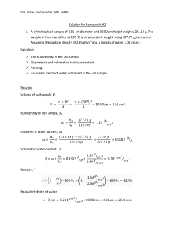


© Copyright 2026