
U ’ M SER
CAMBRIDGE ENGINEERING SELECTOR
Version 3.2
USER’S MANUAL
Granta Design Limited
Cambridge Engineering Selector v3.2 User’s Manual
Release 1
D. Cebon, M.F. Ashby, L. Lee–Shothaman
Copyright © 1999-2001 Granta Design Limited
All Rights Reserved. No part of this publication
may be reproduced, stored in a retrieval system,
or transmitted in any form or by any means,
electronic or otherwise, without the prior
permission of the Copyright owners and the
Publisher.
First edition printed 2001, Granta Design Limited.
Microsoft, Windows 95, 98, 2000 and Windows NT are trademarks of Microsoft Corporation.
Contents
Legal Matters ........................................................................................................... iv
Licence Agreement...................................................................................... iv
Copyright..................................................................................................... iv
Trademarks ................................................................................................. iv
Permission to Reprint, Acknowledgements, References........................... iv
Part 1 Introduction, Installation ....................................................................................... 1
Chapter 1 Introduction ........................................................................................... 1
1.1 Read this First!....................................................................................... 1
1.2 Organisation of the Manual ................................................................. 1
1.3 Tutorials and Reference Information .................................................. 2
1.4 Obtaining Help...................................................................................... 2
1.5 Mouse Buttons ...................................................................................... 2
1.6 Typographical Conventions ................................................................. 3
1.7 The Toolbars ......................................................................................... 3
1.8 What’s New in CES3.2 .......................................................................... 4
Chapter 2 Installation.............................................................................................. 9
2.1 Introduction .......................................................................................... 9
2.2 Running the Setup Program............................................................... 10
2.3 Registering Your Copy of CES Selector ............................................. 10
2.4 Installation .......................................................................................... 12
2.5 Multiple User Installations ................................................................. 15
2.6 Purchasing Additional Data Modules................................................ 16
2.7 Re–Registering your Software ............................................................ 16
Part 2 Selection ................................................................................................................. 17
Chapter 3 CES Selector Concepts......................................................................... 19
3.1 Architecture......................................................................................... 19
3.2 Database Concepts .............................................................................. 20
3.3 Types of Data....................................................................................... 24
3.4 Data Types in Selections ..................................................................... 26
3.5 Sources of Data.................................................................................... 26
3.6 Estimated and Not-Applicable Attributes ......................................... 26
3.7 Selection Methodology ....................................................................... 27
Chapter 4 Data Modules ....................................................................................... 29
4.1 Materials .............................................................................................. 29
4.2 Manufacturing Processes .................................................................... 31
4.3 Structural Sections .............................................................................. 34
Chapter 5 Selector Quick Start Guide .................................................................. 39
5.1 Introduction ........................................................................................ 39
5.2 Getting Started .................................................................................... 39
5.3 The Database ....................................................................................... 44
5.4 The On–line Books ............................................................................. 51
5.5 Selection............................................................................................... 55
5.6 Further Facilities ................................................................................. 62
5.7 Concluding Remarks .......................................................................... 69
ii
CES User’s Manual
Part 3 Construction .......................................................................................................... 71
Chapter 6 Selection Database Design ................................................................... 73
6.1 Introduction ......................................................................................73
6.2 Database Taxonomy ........................................................................... 73
6.3 Comprehensiveness............................................................................. 74
6.4 Universal Attributes ............................................................................ 74
6.5 Two-step Screening and Ranking Process ......................................... 75
6.6 Forms and Filters................................................................................. 75
6.7 Completeness....................................................................................... 76
6.8 Data Quantity and Precision .............................................................. 76
6.9 Choice of Fields ................................................................................... 76
6.10 Data Checking ................................................................................... 77
6.11 Approximations, Estimates and Non-Existence of Data ................ 80
6.12 Relational Structures ......................................................................... 81
6.13 Supporting Data Tables.....................................................................81
6.14 Conclusions ....................................................................................... 83
Chapter 7 Constructor Quick Start Guide ............................................................ 85
7.1 Introduction ........................................................................................ 85
7.2 Editing Attributes ................................................................................ 85
7.3 Adding Records ................................................................................... 90
7.4 Creating Table Components............................................................... 95
7.5 Creating a New Table .......................................................................... 99
7.6 Conclusions ....................................................................................... 107
Chapter 8 Advanced Construction Features ...................................................... 109
8.1 Links................................................................................................... 109
8.2 Automatic Data Checking: Implementation Details....................... 111
8.3 Constants and Parameters ................................................................ 113
8.4 Units and Currency........................................................................... 115
8.5 Creating Functional Attributes......................................................... 121
8.6 Importing Data.................................................................................. 125
8.7 Copying and Updating...................................................................... 134
8.8 Conclusions ....................................................................................... 140
Appendices ....................................................................................................................... 141
Appendix A – Toolbars ........................................................................................ 143
A1 Selector .............................................................................................. 143
A2 Selector and Constructor ................................................................ 143
A3 Constructor ...................................................................................... 144
Appendix B – Filter Settings................................................................................. 145
B1 Materials Selection ............................................................................. 145
B2 Process Selection ................................................................................ 145
B3 Structural Sections Selection ............................................................. 145
Appendix C – General Information..................................................................... 146
C1 File Types ........................................................................................... 146
C2 Limits on Data Types ........................................................................ 147
C3 Naming Conventions ........................................................................ 148
C4 Constructor Options for Preferred Currency and Units ................. 149
Contents
iii
Appendix D – Functional Data Syntax ............................................................... 150
D1 Description of Functional Data Syntax ........................................... 150
D2 Expression Function ....................................................................... 150
D3 Array Function ................................................................................ 151
D4 Estimated Functional Attribute ....................................................... 152
D5 Functional Range Examples ........................................................... 152
D6 Functional Point Examples .............................................................. 154
D7 Example Files..................................................................................... 156
Appendix E – References...................................................................................... 157
Index ..................................................................................................................... 158
Legal Matters
Licence Agreement
The software described in this document is furnished under a Licence Agreement and
may be used or copied only in accordance with the terms of the Licence.
Copyright
This documentation for the Cambridge Engineering Selector (CES) and the software
described in it are copyrighted © 1999-2001 Granta Design Limited, with all rights
reserved. Under the copyright laws, neither the documentation nor the software may be
copied, photocopied, reproduced, translated, or reduced to any electronic medium or
machine readable form, in whole or in part, without the prior written consent of Granta
Design Limited, except in the manner described in the installation instructions.
Trademarks
Cambridge Engineering Selector, CES Selector, CES Constructor, CES Viewer,
CES InDepth and CES Weblinks are Trademarks of Granta Design Limited.
Permission to Reprint, Acknowledgements, References
Reprinting
Selection charts, attribute data and extracts from hardcopy or on-line documentation,
copyrighted by Granta Design Limited may be reprinted in published works provided:
(i) prior written permission is obtained for every instance from Granta Design Limited
by mail, fax or electronic mail (contact details on back cover of this manual);
(ii) each such chart, attribute list, document, etc is accompanied by an acknowledgement
of the form
“Chart/data/etc from the Cambridge Engineering Selector, v3.2, Granta Design
Limited, Cambridge, UK, 2001.”
Bibliographic References
When referring to the CES software in publications, the bibliographic reference is:
“Cambridge Engineering Selector v3.2, Granta Design Limited, Cambridge, UK,
2001.”
When referring to this User’s Manual in publications, the bibliographic reference is:
“Cebon, D. Ashby, M.F. and Lee–Shothaman, L ‘Cambridge Engineering Selector
v3.2 User’s Manual’, Release 1, Granta Design Limited, Cambridge, UK, 2001.”
PART 1
INTRODUCTION,
INSTALLATION
Chapter 1 Introduction
1.1 Read this First!
The Cambridge Engineering Selector (CES) is a powerful tool. It has two main
components: Selector and Constructor. Selector incorporates a set of eight data tables
(materials, manufacturing processes, shape, structural sections, suppliers, references,
uses and industrial sectors). Additional tables can be purchased separately. These tables
are linked together in a relational structure to provide a powerful engineering selection
system. They contain unique sets of high quality data, developed by Granta’s specialist
database team, in conjunction with Cambridge University Engineering Department.
Selector contains a powerful selection methodology for choosing entities to optimise
performance, based on design specifications.
It is possible to use the selection facilities of Selector without knowing the finer details of
the selection methodology. However, you will only benefit from the full power of the
package to optimise selections if you take a little time to read about it in Chapter 3 of this
manual (CES Concepts) and in the Background Reading section of the on-line book
‘CES InDepth’. We also recommend that you read the Selector Quick Start Guide
(Chapter 5 of this manual), and that you work through some of the Tutorials on how to
use the package in the on-line Help system.
CES Constructor is a tool for making and editing selection databases for use in Selector.
In order to work well for optimal selection, databases need to have a number of special
characteristics. Some of the background to database design is provided in Chapter 6.
The Constructor Quick Start Guide in Chapter 7 illustrates a number of the important
features of Constructor, and Chapter 8 expands upon some of the more technical aspects
of the package. To learn about the remaining facilities, we recommend that you work
through the comprehensive set of Tutorials in the on–line Help system.
1.2 Organisation of the Manual
This manual contains eight Chapters:
Part 1 Introduction, Installation
Chapter
1
Introduction
Chapter 2 Installation
provides some general information about
obtaining help, using the mouse, typographical
conventions in this manual, and the ‘docking’
toolbars in Selector and Constructor.
gives step–by–step instructions on how to install
single– user and multi–user copies of CES.
2
CES User’s Manual
Part 2 Selection
Chapter 3 CES Concepts
explains the basic concepts and definitions
underlying the organisation of CES databases and
the selection methodology.
Chapter 4 Data Modules
describes the contents of the three core selection
data tables in the CES system: Material, Process
and Structural Sections.
Chapter 5 Selector Quick Start
provides a brief overview of the facilities of CES in
tutorial format.
Part 3 Construction
Chapter 6 Database Design
discusses the design of selection databases: their
structure and important features.
Chapter 7 Constructor Quick Start provides tutorials on the use of some of the key
features of Constructor.
Chapter 8 Advanced Features
discusses some of the more technical aspects of
CES Constructor: in particular, links, data checking
and importing data from external files.
1.3 Tutorials and Reference Information
A comprehensive set of tutorials on use of Selector and Constructor as well as reference
information about all aspect of the software can be found in the on-line Help system.
The on-line book ‘CES InDepth’ contains a wealth of information about the CES system,
including details of the selection methodology, definitions of all attributes in the
database, 50 interactive case studies, and supporting information including solutions to
many standard engineering problems, tables of equivalent material designations, etc.
1.4 Obtaining Help
Help can be obtained in Selector and Constructor in three different ways:
(i)
Select the Contents option from the Help pull–down menu at the top of the
CES screen.
(ii)
Click on the Help button
(iii)
Press function key F1 at any time to obtain context–sensitive Help.
on the standard toolbar.
1.5 Mouse Buttons
One click of the left mouse button is used for selecting objects and menu options in
Selector and Constructor. Double-clicks of the left mouse button normally invoke the
default action for a particular object. For example, double-clicking on the name of an
entity in the Selection Results window of Selector presents a list of the entity’s attributes.
Chapter 1 Introduction
3
The right mouse button can be used throughout CES to obtain ‘shortcut’ or ‘context’
menus for an object. These menus shows the most frequently used commands for that
object. The first item on the context menu is often the default action (see figure 1.1
below).
Click right mouse button while
pointing cursor at this object
'Context' menu of
options appears
Click left mouse button
to select this option
Fig. 1.1 ‘Shortcut’ or ‘Context’ menu. This one was obtained by clicking the right mouse button on the
Magnesium/Wrought branch of the CES Materials tree.
1.6 Typographical Conventions
• Instructions that you should follow in the Installation Manual and Quick Start Guides
are denoted by indented text in boldface, such as the following line:
This is the format of an instruction
• The names of menu options and buttons in this manual appear in boldface.
• Sub–menus are written with forward slashes ‘/’ separating items: ‘View/Results’ means
the Results option on the View menu.
• The names of windows and dialog boxes appear in italics, eg Project window.
• Items of text contained in list boxes appear in ‘quotation marks’.
• Words and numbers that you type as you follow the instructions are underlined.
• ↵ means press ENTER.
1.7 The Toolbars
There are several ‘docking’ toolbars available in both Selector and Constructor. They can
be switched–on and off using the Toolbars option on the View menu (View/Toolbars).
‘Docking’ means they can be moved around the screen and placed at convenient
locations, by dragging them with the mouse. When a toolbar is placed against an edge of
4
CES User’s Manual
the program viewing area (the ‘frame’), it will merge into the frame. Another toolbar
placed alongside will merge into the first.
If you place the cursor over a button a ‘tool tip’ will appear. This will give one or two
words of explanation about the function of the button.
Explanations of the various buttons on the toolbars are provided in Appendix A.
1.8 What’s New in CES3.2
This section is only relevant if you have upgraded from CES3.1 to 3.2. For information
about the differences between the Cambridge Materials Selector (CMS) and CES, visit
our web site: www.grantadesign.com/products/diffcmsces.htm.
The major additions in CES 3.2 Selector are the capacity for ‘model-based selection’, that
is, selecting entities using properties which vary with one or more independent
parameters (eg, variation of elastic modulus with temperature); data export to finite
element analysis packages; process cost modelling, enabling selection of processes on cost
criteria; substantially extended information about polymers and polymer composites;
information about tool steels and magnetic properties of materials, as well as extensive
information about trade names, equivalent designations, chemical compositions, and
numerous other features. CES Constructor has been enhanced with a variety of new
facilities, including sophisticated database copying and merging facilities and the
Weblinks Manager system for managing linkage to web searching.
There is now also an option to have the Military Handbook data (MIL-HDBK-5 and
MIL-HDBK-17) included in CES 3.2, making it particularly relevant to aerospace and
defence industries.
The enhancements in CES 3.2 are described in detail in the following sub-sections.
1.8.1 CES Selector
Model-Based Selection.
Model-based selection is the software capability in CES that enables selections based on
‘functional data’. Functional data describes properties that vary with one or more
independent parameters eg ‘Modulus with Temperature’ or ‘Fatigue Strength with No. of
Cycles and Stress Ratio’. Model-based selection allows selections to be made through
manipulation of this type of data. Example: On a chart of Density vs Modulus with
Temperature, the user can change the specified temperature. The software automatically
changes the value of Modulus for each material accordingly.
This versatile capability can be used to store many kinds of functional data e.g. creep,
fatigue, deformation mechanism maps, variation of properties with temperature etc.
Export to FE Packages
An export capability to some of the major Finite Element Analysis (FE) packages has
been developed. Currently data can be exported to: ABAQUS, ANSYS, NASTRAN,
PATRAN.
Chapter 1 Introduction
5
Full Text Searching
The new search facility means that users can search across all text properties in any of the
data tables in the database e.g. trade names, typical uses.
Composition Searching
A new Form, ‘Composition’ contains the composition details for each of the materials in
the database. This can be used to select materials not just on their properties but also
based on their composition. This is also fully compatible with the full text search facility
(above).
Axis range – Charts
The user can now specify axes range for selection charts. Previously the axes range was
fixed, at the maximum and minimum values of the displayed data.
Elongation
The property used to describe how much a material can stretch before breaking has been
changed from ‘ductility’ to ‘elongation’. The two are identical, except that elongation is
expressed as percentage instead of a fraction, e.g. ductility of 0.1 equates to an elongation
of 10%.
Hide Non-Applicable Properties
When viewing data sheets in CES, if there is no data for a particular property the message
“Not Applicable” is displayed. It is now possible to hide these properties so that only
properties that have values are displayed. The control for this option is in Tools/Options
on the menu.
‘All Bulk Materials’ Filter
The default filter in Selector is now referred to as ‘All Bulk Materials’. It contains all
materials in CES with the exception of some that are considered not suitable for making
engineered products. (Examples include commercially pure metals, the less common
woods, reinforcement fibres, particulates, and some natural materials such as bone.) The
filter ‘All Materials’ contains all the material records in the CES materials data module.
1.8.2 CES Constructor
The power of CES Constructor has been greatly enhanced with sophisticated software
tools which enable database managers to copy and manipulate their in-house data and
merge it with reference data sources.
Model-Based Selection
It is now possible to store Functional data in CES Constructor, either as a mathematical
function or as an array of points.
New Data Types
Five new data types are available in CES databases. These are functional range,
functional point, integer, date and hyperlink (URL). All except hyperlinks can be used in
selections.
6
CES User’s Manual
Expanded Table Size
The limit on the number of fields in a CES table (previously 256) has been removed.
CES tables can now contain any number of fields.
CES Weblinks Manager
CES Weblinks Manager is a facility in CES Constructor that enables the user to edit the
Weblinks database (a database of relevant web sites) to keep it relevant and up-to-date,
and upload the database to CES Weblinks Server. CES Weblinks Manager can
automatically store web site addresses (which are entered by drag and drop from a web
browser) and link them to other related records in the database.
CES Weblinks Server is available for purchase separately. Please contact Granta Design
for further information.
1.8.3 Materials Data Module
Polymers
The Polymer section of the materials table has been completely revised and updated. It
now contains over 500 records covering filled and unfilled polymeric grades and covers
the vast majority of commercially available polymers
Fifteen new polymer-related attributes have been added:
Compressive Modulus
Hardness - Rockwell M
Linear Mould Shrinkage
Processing Temp. (Compression)
Processing Temp. (Injection)
Transparency
Polymer Type
% filler
Flexural Modulus
Hardness - Rockwell R
Moulding Pressure Range
Processing Temp. (Extrusion)
Dissipation Factor
Tradenames
Filler Type
Polymer Composites
Information for 25 polymer matrix lamina and laminate composites has been added to
the data module. The properties for quasi-isotropic (QI) laminates are given for all
composite materials.
Base data is included for both non-woven and woven materials. The base properties for
the non-woven materials are given for unidirectional laminates in the longitudinal and
transverse directions. For the woven materials, the properties for biaxial laminates are
used. Where data was taken from the MIL-HDBK-17, links to MIL-HDBK-17 test data
information have been added (requires the optional separate MIL-HDBK database for
this to work).
Tool Steels
The materials table has been enhanced with records covering 82 Tool Steels. Additional
properties appropriate for the specific properties of tool steels have been added. These
properties allow the selection criteria to reflect the needs of tool tip materials. Examples
Chapter 1 Introduction
7
include: Decarburisation Resistance, Distortion Resistance Rating and Cracking
Resistance Rating.
The new tool steel materials are shown in the ‘Tool Steels’ filter.
Magnetic Materials
Records for 50 hard and soft magnetic materials have been added to the materials data
module. The entries are split between electromagnets (soft magnets) and permanent
magnets (hard magnets). Specific properties including maximum permeability, coercive
force, remnant induction and saturation induction have been added to some existing
records for soft magnets. For the hard magnets, data is available for remnant induction,
coercive force, intrinsic coercive force, maximum energy product and recoil
permeability. In addition, details of the temperature dependence of the above properties
are available for some materials.
The magnetic materials and their specific properties are shown in the ‘Magnetic’ filter
and form.
Aluminium-Beryllium
Aluminium-Beryllium (AlBeMet) alloy has been added to the database. This is an
important new material for high-end, light-stiff applications.
Trade Names and Equivalent Standards Designations
These have been extensively revised and updated in co-operation with ASM
International and now cover 47 standards organisations in 40 countries. CES includes
approximately 8,000 material equivalencies.
Fatigue Strength
A Fatigue Strength model property (known as an S-N curve) has been included for the
metal records in CES. This is a generic fatigue model, constructed by Granta Design to
estimate the fatigue strength based on the variables ‘No. of Cycles’ and ‘Stress Ratio’, the
values of which can be changed by the user.
Hardness
The generic hardness property (i.e. given for all materials) has changed from ‘Hardness’
to ‘Hardness – Vickers’. Vickers hardness is a known engineering property. The
previously used hardness was a stress equivalent, effectively a factor of 10 greater.
Note: Alternative hardness systems are available for some materials where relevant, e.g.
Rockwell M and R for polymers, Rockwell C for tool steels.
Transparency
All materials are now ranked on four levels of transparency: Opaque, Translucent,
Transparent and Optical Quality.
The old logical property ‘opaque’ for ceramics has been deleted.
MIL-HDBK data
The materials module within the CES 3.2 standard database includes records for all of
the MIL-HDBK-5 materials. These records do not carry any statistical traceability and
8
CES User’s Manual
include information from other sources. Similarly, records have also been included for
generic unidirectional (UD), biaxial (BI) and quasi-isotropic (QI) laminates fabricated
from composite materials from MIL-HDBK-17. These database updates allow materials
contained within two major sources of aerospace specific information to be compared
and contrasted with the widest range of possibilities. The original data in MIL-HDBK-5
and MIL-HDBK-17 can be accessed via separate optional CES tables.
Direct access to the MIL-HDBK-5 PDF files is provided for all of the appropriate
materials via the CES Weblinks system. The links allow the exact section of a PDF file to
located easily, directly from a materials record in CES, increasing the availability and
value of this information source, as well as providing traceability information for the
MIL-5 material data.
Unit Systems
Two new self-consistent Imperial unit systems have been introduced for the FE export
facility. The two systems are FPS (Consistent) and IPS (Consistent). For these two unit
systems all lengths are expressed in feet (ft) or inches (in) and masses in pounds (lbs).
1.8.4 Process Data Module
Cost Index
A model-based property called ‘Cost Index’ has been added for each of the processes in
the database. This property contains a process cost model, which provides an estimate of
the relative cost of making a component by the process as a function of parameters such
as batch size, overhead rate and tooling cost. The cost model is a mathematical function
of resource consumption.
1.8.5 Structural Sections Data Module
The data on Structural Sections, previously stored in the Shape table, has been moved to
its own table.
1.8.6 MIL-HDBK Data Module
The CES MIL-HDBK Data module is available as a separate add-on to existing CES 3.2
software installations. This database contains data from the two Handbooks, MILHDBK-5 (Metallic Materials and Elements for Aerospace Vehicle Structure) and MILHDBK-17 (Composite Materials).
The MIL-HDBK-5 data is reproduced with the minimum of changes. The A, B and S
basis statistical traceability is maintained. All CES records are linked directly with the
appropriate pages in the published MIL-HDBK-5 PDF file on Granta Design’s web site.
This enables the relevant data sheets and sections of the handbook for each material to be
located rapidly in CES using the Weblinks system.
The MIL-HDBK-17 data is stored in records for each combination of materials. The
original data is available unchanged. Additional derived data records have been
generated by manipulating the original raw laminae data using standard composite
mechanics. These records, easily identifiable, and stored in a separate data table, have
been compiled from the detailed ones by experts at Granta Design in order to allow
greater value to be extracted from MIL-HDBK-17 by CES users.
Chapter 2 Installation
2.1 Introduction
This part of the User’s Manual provides instructions for registering and installing your
copy of CES 3.2.
2.1.1 System Requirements
In order to run CES 3.2, your personal computer (PC) must have the Windows™
operating system (Windows 95, 98, 2000 or Windows NT4, service pack 3 or later) and
should have at least a Pentium II processor (or equivalent) with 32MB of RAM and
SVGA graphics (256 colour, 800x600), mouse or compatible pointing device. A
‘compact’ installation of a single user licensed copy will need at least 300MB free hard
disk space and 4X CD-ROM drive. A full installation will require around 400MB free
hard disk space. An Internet connection is required for running CES Weblinks.
You may need Administrator Rights to install the software.
2.1.2 Licence Options
The CES Licence Agreement specifies the number of ‘users’ or ‘seats’. This is the
number of computers on which the software may be installed.
If the Licence is for a Single User, then the software may be installed on one personal
computer only. Installation on more than one computer or installation on a network
drive is forbidden under the terms of the Licence.
If the Licence is for Multiple Users (multiple ‘seats’) the software may be installed on the
number of computers specified on the Licence Agreement. Note that such installations
may use a network drive to store a single common copy of the database.
2.1.3 Configuration
For a single-seat licence, the program must be installed on the hard disk drive of a PC.
With multiple-seat licences (eg teaching licence or office licence), the program must be
installed on each PC. In network installations, this can be done using the ‘netsetup’
program which is supplied with the software. Each networked PC must have access to
some ‘writeable’ file space, either on a local hard disk or on a network file server.
Network installations are discussed in Section 2.5.
All CES data modules are installed by the installation procedure described in the
following sections. Additional CES data modules can be purchased and installed in the
same way.
10
CES User’s Manual
2.2 Running the Setup Program
If you have installed a copy of CES Selector Evaluation, it is recommended that you un–
install this before installing your licensed copy.
CES uses a Setup program similar to those of many other Windows™ applications. You
can proceed through the stages of installation by clicking once with the left mouse button
on the Next or Yes buttons. You can stop the installation process whenever a Cancel
or Exit Setup button is displayed. A Back button will take you back to the previous
stage.
Insert the disk in your CD-ROM drive
The Setup program should run by itself. If it does not, try one of the following actions:
Open Windows Explorer and double-click on the file Setup.exe on your CDROM drive
or use the Windows™ ‘Run’ command as follows:
From the Windows™ Start menu, select the ‘Run’ command
This will open the Windows™ ‘Run’ dialog box, as shown in figure 2.1.
Fig. 2.1
The Windows™ Run dialog box
Click in the Open field in the Run dialog box, then type E:\Setup
where E:\ is the location of the Setup.exe file (your CD–ROM drive).
Click once on OK.
If one of the above procedures has been successful, after a few seconds, you should see
the Welcome dialog box (figure 2.2).
Click on the Next > button
2.3 Registering Your Copy of CES Selector
To register your copy of CES Selector, enter the relevant details for your Name, Company
and registration Key (see figure 2.3). A Name is required. Your registration key is
provided on the Licence Agreement card that accompanied the software.
Chapter 2 Installation
Fig. 2.2
The Welcome dialog
Fig. 2.3
Registration information
11
12
CES User’s Manual
Enter your Name and Company details
Enter your registration key (located on your Licence Agreement card) by
typing it in the field provided
Click once on Next > to confirm the registration information and continue
with the setup procedure
The Licence Agreement screen will appear (figure 2.4). The Licence Agreement is a
legally binding agreement between you and Granta Design Limited. The same Licence
Agreement text appears on the Licence Card. For ‘Customer’ details, the ‘Site’ and any
special conditions, please see the hard copy Licence Card.
IF YOU CLICK ON THE I Agree BUTTON, YOU AGREE TO BE BOUND BY THE
TERMS OF THE LICENCE AGREEMENT AS SPECIFIED ON THE LICENCE
AGREEMENT SCREEN AND ON THE LICENCE CARD.
Once you have read the licence agreement, you can proceed with installing CES Selector:
Click once on the I Agree button, if you agree to be bound by the terms of the
Licence Agreement.
Fig. 2.4
The Licence Agreement
2.4 Installation
The remaining information required for installation is the location and the software
components to be installed. The default installation location is a directory called
C:\Program Files\CES Selector 3.2. You do not have to create the default directory
beforehand, the setup program will create it for you.
Chapter 2 Installation
13
If you wish to change the destination location for your copy of CES Selector:
Click once on the Browse button on the ‘Choose Destination Location’ dialog
box (figure 2.5). Select a folder in the ‘Select Destination Directory’ dialog and
then click once on OK
When you are happy with the destination,
Click once on the Next > button.
The ‘Select Components’ dialog will appear (figure 2.6). This screen informs you about
some details of your Licence (including the components that will be installed) and
enables you to choose between a Full and Compact installation.
A Full installation will install all of the components, including the on-line books. You
will use about 400 MB of hard disk space for the CES Engineer Pro package (less for the
other packages). A Compact installation will install all the components needed to run
CES Selector, but you will need to use the CD-ROM to view the on-line books. It will use
about 300 MB of hard disk space for the CES Engineer Pro package.
We recommend that you do a Full installation if possible.
Fig. 2.5 Choose destination for software
14
CES User’s Manual
Fig. 2.6
Select installation components
Select an Installation option by clicking once on the button for ‘Full’ or
‘Compact’
Click on the Next > button in this dialog box and in the following dialog box
to perform the installation – or click on < Back if you wish to alter any of the
installation settings.
A ‘thermometer’ indicator will inform you of the progress of the installation.
When Setup has finished, a dialog box will appear with the message ‘Cambridge
Engineering Selector has been successfully installed.’
Click on OK to exit the installation program.
The program will return control to Windows™.
The installation process will make a Start Menu Program group called ‘CES Selector’,
which will contain the icons for CES software components, as shown in figure 2.7
Double-click on the ‘CES Selector’ icon to perform selections, or
‘CES Constructor’ to create/edit selection databases.
Uninstall the entire system by double-clicking on ‘Uninstall CES Selector’
You can also access the CES Selector Start Menu Program group from the Programs
option on the Start menu (on the Windows™ task bar).
Chapter 2 Installation
Fig. 2.7
15
The CES Selector group in Windows Program Manager
Note that the CES Constructor software is not automatically distributed with every
CES system. It will only be available if you have purchased a licence for Constructor.
2.5 Multiple User Installations
This section provides information about options for multiple-user installations of CES
Selector. It assumes that you have some experience with setting up Windows programs
to run on networks.
Multiple–user copies of CES Selector can be installed in two possible ways. In both cases
it is necessary to perform an installation on every machine on which the software is to be
used.
(i)
CES Selector can be installed individually on the hard disk drive of every machine
on which it will be used, i.e. like a single-user installation. In this case, you
should follow the installation instructions described in the previous sections, and
install the software into a folder on the local hard disk. If more than one copy is
to be used simultaneously, a ‘full’ installation will be required on each machine,
so as to enable access to the on-line books.
(ii)
The software can be installed in a folder on a network drive. In this case, you
should follow the installation instructions described in the previous sections, but
install the software into a folder on a network drive that is read–accessible to all
PCs on the network. A ‘full’ installation will be required on the network drive if
the users are to have access to the on-line books. The netsetup program can then
be run on each PC on the network to install the relevant ‘client’ components of
the software.
In both cases, users will require some file space with ‘write’ access, for saving CES output
and project files.
2.5.1 Example 1
You are a commercial user and have purchased an office licence. The system
administration decides to install the software individually for each user. The software is
to be used on five different machines. For each machine, a Full installation to the local
hard disk drive must be carried out from the CD-ROM.
16
CES User’s Manual
2.5.2 Example 2
You are an educational user and have purchased a teaching licence. All of the 20 PCs in
the lab are networked to a file server. The hard disk drive of each PC is the ‘C’ drive.
The network drive ‘F’ can be read by the networked PCs. Only the system
administrator has write access to this drive. The system administrator runs the setup
program and performs a ‘full’ installation to the folder F:\CES Selector, and also copies
the netsetup.exe program to the folder F:\CES Selector. Then on each of the 20 PCs in
the network, the administrator runs the netsetup.exe program
F:\CES Selector\netsetup.exe. This will install program files and dll’s to the local
machine, but the database and the on-line books will be accessed from the server
location. A user of CES Selector at one of the networked PCs must have read permission
for the F drive and write permission to a folder on the network or on PC they are
currently using, for output of CES files (eg C:\Users).
Notes:
(i)
None of the ‘.exe’ files (other than the netsetup.exe) or ‘.dll’ files are required in
the server installation directory, unless CES is going to be run by a local user on
the server machine.
(ii)
CES requires certain system dll’s to run. If a compatible version of these files is
not found on the user’s machine, and the machine is running Windows NT, then
user will need to have Administrator rights to install the software – or the
installation may fail.
2.6 Purchasing Additional Data Modules
Upon purchase of additional data modules, Granta Design Limited (or their accredited
agent) will provide a new registration key. To install and register an additional data
module, follow the instructions which come with the new module. If you have a multiuser licence and have installed to a network drive which is accessed by all the networked
PCs for which you are licensed, you will only need to run the Setup program once.
2.7 Re–Registering your Software
If you need to re-register your software (for example, if you obtain a new licence for an
extended time period or different number of users), use the Licence Key option on the
Tools menu of CES Selector or CES Constructor to open the Licence Key dialog. Simply
enter the new key in the input field provided.
PART 2
SELECTION
Chapter 3 CES Selector Concepts
3.1 Architecture
The CES system is a linked set of modules, as shown in figure 3.1. The selection is
design-led, meaning that the inputs are the design requirements. These are translated
into a prescription for selecting material and process properties.
CES Selector is the central module of the CES system. It enables engineers to select, from
relational databases, a small subset of entities which optimally satisfy the requirements of
a design. The selections may be performed using the CES materials, manufacturing
processes or structural sections data modules. Alternatively they may be performed on
user-databases developed with CES Constructor.
Design
Specification
CES
Other
information
sources
Selection
databases
CES database
Selector
M
Constructor
P
CDÐROMs
(CES Viewer)
S
Shape
Process
Material
Prop 1 1.3 - 1.4
Prop 2 2.4 - 2.5
Prop 3 T
Prop 4 F
Prop 5 A
Prop 6 E
User database
Prop 1 1.3 - 1.4
Prop 2 2.4 - 2.5
Prop 3 T
Prop 4 F
Prop 5 A
Prop 6 E
Internet
(CES Weblinks)
Entity 123
Prop 1
Prop 2
Prop 3
Other Databases
The Selection
Fig. 3.1
Architecture of the CES System
3.1.1 Screening and Ranking
CES Selector treats all members of the databases as potential candidates until, by
screening, they are shown to be unsuitable. As a consequence, viable candidates cannot
be overlooked. This screening can be based on simple go/no-go criteria: has the material
a sufficiently large modulus? Is the process able to cope with that material? More
revealing, often, is to create a sequence of selection charts which give a visual picture of
the important attributes of the material or process. Often it is not a single property that
counts; rather, it is some combination of them. The Selector creates any combination of
20
CES User’s Manual
properties you wish and allows you to screen and rank the candidates with them. CES
Selector provides a number of other tools to facilitate sophisticated optimisation
strategies, and it automatically keeps track of the selection results.
3.1.2 Supporting Information
Screening and ranking based on numeric properties are merely the first steps in any
selection exercise. They deliver a ranked list of potential candidates, but this can be long,
and with many questions unanswered. Once a subset of entities is found, CES Selector
provides automatic access to vast sources of supporting information: searchable files or
databases provided by Granta or others on CD-ROM; text, images and tabular data of
the sort found in handbooks; and immediate Internet access to an enormous range of
material and process information through the CES Weblinks system. This gives
background reference information for the short-listed candidates: their reputation; case
histories of their uses; warnings about their weaknesses; the environmental consequences
of their use, supplier data, etc. This supporting information can be used to narrow–
down the short list of candidates to a final choice.
3.2 Database Concepts
3.2.1 Database
In CES, a database consists of one or more tables (datasets) which are linked together.
The complete CES database has eight linked tables, as shown in figure 3.2. The main
selection tables contain materials, manufacturing processes, and structural sections. The
supporting tables contain information about suppliers, references (the sources of
information that were used to compile the main tables), as well as shape (used in process
selection), uses of materials and application areas. The main selection tables are detailed
in Chapter 4 of this User’s manual.
USES
APPLICATION
AREAS
SUPPLIER
MATERIAL
PROCESS
REFERENCE
Fig. 3.2
STRUCTURAL
SECTIONS
SHAPE
CES database structure. The circles represents tables. The lines joining tables represent links.
Chapter 3 CES Selector Concepts
21
3.2.2 Tables
A Table is a compilation of information relevant to a single type of entities (records).
For example, it may contain materials and their properties, or manufacturing processes.
A table can be thought of as one page of a spread sheet: with records (eg materials) in
each row and a set of attributes (sometimes called properties, or ‘fields’) in the columns.
Each table in the current database is listed in the drop-down list on the Tables tab in the
Project window of CES (figure 3.3). The records in each table are arranged into a
hierarchical ‘classification tree’ structure. Select the name of a table from the list to view
its tree.
Online books
Select the Materials
Table from the list
Generic record
Specific record
Folder record
Fig. 3.3
The Project Window, showing the Materials table and part of the materials classification tree.
CES Selector v3.2 can only perform selections on one table at a time – for example
materials or processes. This table is called the Selection Table. The Selection Table is set
for the current CES ‘Project’. If you change selection table, you must start a new project.
22
CES User’s Manual
3.2.3 Records and Attributes
Each record in the database represents an entity – a material, a process, a supplier, etc.
Each record has a set of attributes. For a material record, these attributes include its
composition, strength, density etc. For a manufacturing process record, the attributes
include the surface finish, tolerance, economic batch size etc. For a supplier, the
attributes are the Company name, address, telephone number, etc.
The attributes of a record can be viewed in the Attributes window (see figure 3.4).
Fig. 3.4
The Attributes window, showing some properties of the record Aluminium Alloy 2014–T6.
3.2.4 Folders
Every record in the database has a unique ‘Identifier’ (ID), which is used to distinguish it
from all other records. The records are organised into a hierarchical ‘tree’ structure,
known as an ‘identifier tree’ or ‘table tree’. Individual records are the ‘leaves’ of the
table tree. Part of the Materials Table tree can be seen in figure 3.3.
acts as a branch of the tree. It does not have any attribute data
A folder record
associated with it, but does have records ‘below’ it in the tree.
is a record whose attributes span the range of attributes of a number
A generic record
of specific records. It is a ‘fictitious’ entity that represents the properties of the records
below it in the tree (eg ‘Wrought Aluminium Alloys’ in figure 3.3). Generic records are
Chapter 3 CES Selector Concepts
23
particularly useful during the early stages of the selection, where breadth of information,
and not detail is important.
represents a ‘real’ entity (eg Aluminium alloy 2014–T4). It is not
A specific record
usually possible to subdivide a specific.
3.2.5 Record Identifiers
Record Identifiers consist of several pairs of letters (sometimes including blanks ‘_ ’ ).
The first character of the identifier indicates which table it belongs to (M means
Materials, P means Process etc). Subsequent letters denote the family, class and sub–
class, followed by three numbers which denote the particular member of the sub–class.
The same type of Table tree classification system is common to all CES data tables.
Part of the table tree for Aluminium Alloys is shown in figure 3.3. The identifier
‘MMLAALW–SB001’ can be ‘decoded’ as follows:
MM
LA
AL
W_
SB
001
Material, Metal
Light Alloy
Aluminium
Wrought alloys
2000 series
2000 series alloy number 001 in the CES designation system.
See CES InDepth for details of the identifier trees in each data table.
3.2.6 Filters
A Filter is a device for specifying which records in a table are visible.
The current record filter for each table can be viewed and set in the Table Properties
dialog. The filter for the current Selection Table is visible on the Filters toolbar
(figure 3.5).
Fig. 3.5
The Filters toolbar, showing the form and filter set for the Selection Table.
A set of pre-defined filters is available for each table, and is available in a list box
wherever the filter setting can be changed. It is also possible to ‘expand’ and ‘contract’
generic records, so as to add or remove records from the current filter. In this case, the
filter automatically becomes called ‘<User Defined>‘.
The record filter for the Selection Table determines which records are available for
selection.
3.2.7 Forms
A form is a template that specifies the attributes that are visible and their layout in the
Attributes window.
Some attributes are relevant to all entities in the table, others are specific to a particular
class of entities. For example ‘Density’ is a relevant attribute for all material records,
whereas ‘Water Absorption’ is only relevant for a particular class of materials: Polymers.
24
CES User’s Manual
The ‘Generic’ Form, (which is the default form for the Materials table, and is relevant for
all classes of materials), contains Density, but not Water Absorption. The ‘Polymers’
form contains both Density and Water Absorption.
A set of pre-defined forms is available for each table in a list box wherever the form
setting can be changed. The current form for each table can be viewed and changed in
the Table Properties dialog. The form for the Selection table is also visible on the Filters
toolbar (figure 3.5).
The record form for the Selection Table also determines the attributes that are available
for selection purposes. Following the example above, it is only possible to use ‘Water
Absorption’ as a selection criterion if the current Form is set to Polymers.
Forms can only be designed or modified in CES Constructor (not in CES Selector).
3.3 Types of Data
Each record has a number of attributes that are stored in fields in the database. The
attribute data can be one of the following types. (See details in Appendix C2).
3.3.1 Numerical data
Numerical attributes can be stored as a range, a point or an integeror as functional data.
Range, Point and Integer
For attributes stored as a range, a minimum and maximum value is specified. For
example, in the materials data table, Wrought Aluminium Alloy 2014–T6 has an ‘Elastic
Limit’ in the range 350–440 MPa (figure 3.4). For attributes stored as point values, only
one value is specified. All values are stored to a maximum of 6 significant figures.
Point data can also be stored as integer values, using the ‘integer’ attribute type.
Functional range, Functional point
Functional data describes properties that vary with one or more independent parameters
(see paragraph 3.3.9). The function can either be a mathematical formula or a set of
discrete data points e.g. (x, y, z). Selector evaluates the function at user-specified values
of the parameters. For example: On a selection chart of Young’s Modulus w i t h
Temperature vs Density, the software interpolates a value the modulus at a user–specified
temperature, from an array of data points.
There are two versions of functional data: functional range, which evaluates to a range
attribute and functional point, which evaluates to a point.
3.3.2 Discrete data
Discrete attributes are those where the attribute takes one of a set of discrete values. The
values can be ‘A, B, C, D, E’ or ‘1, 2, 3’ or ‘Red, Green, Blue’ etc. For example the
Environmental Resistance (resistance to standard operating environments) in the
materials data module, takes a value on the five–point scale: ‘Very Poor’, ‘Poor’,
‘Average’, ‘Good’, or ‘Very Good’, (‘Very Good’ means highly resistant to the
environment, and ‘Very Poor’ means completely un–resistant or unstable.)
Chapter 3 CES Selector Concepts
25
The record Identifier (branch of the table tree), can also be considered conceptually as a
discrete attribute for selection purposes.
3.3.3 Logical data
Logical or Boolean attributes are those that are either ‘True’ or ‘False’ (or Yes/No). For
example an attribute in the process data module indicates whether a process class is
‘Primary’ (True) or not (False).
3.3.4 Links
Links between data tables can be considered to be attributes. For example, records in the
Materials data module are linked to records in the Process module.
3.3.5 Text data
Text is stored in fields that can take a short or long string of text. They are used for
qualitative data. For example the attribute ‘Typical Uses’ in the materials data table is of
type ‘long text’.
3.3.6 Picture data
Picture attributes allow the viewing of a diagram or photograph in a record, for example
the ‘Process Schematic’ attribute in the process data table.
3.3.7 Dates
The date data type can be used to store calendar dates.
3.3.8 Hyperlinks
The Hyperlink data type provides a mechanism for storing URL’s (Uniform Resource
Locators), consisting of a protocol and location e.g. ‘http://www.grantadesign.com’
Clicking on the hyperlink in a record in Selector causes the program to open your web
browser and jump to that web page. For example, a material supplier record could have
a dynamic link to the supplier’s web site.
3.3.9 Parameters and Constants
‘Parameters’ and ‘Constants’ are not attributes of database records, however they require
definition.
Parameters
Parameters are the independent variables used to evaluate functional data. For example
the functional attribute ‘Young’s Modulus with Temperature’ contains values of the
Young’s modulus of materials as a function of the parameter ‘Temperature’. Each
parameter has a default value, which is stored in the database.
The default parameters are ‘global’ to a CES project. Their values can be changed, but the
changes have a global effect.
There are two different options for setting the parameter values used to evaluate a
functional attribute – eg when viewing a particular record, or when performing a
selection stage:
26
CES User’s Manual
(i)
The parameter values can be set (‘locally’) for the particular instance of the
function.
(ii)
The (‘global’) project default parameters can be used for viewing the function. If
the project default parameters are used for a selection stage, and the default
parameter values are changed at any time in the current project, the selection
stage will automatically update itself. For example, it would be possible to set the
project default parameter Temperature to a value of (say) 500K (degrees Kelvin).
All material selection stages which used default parameters in functional data
would then be evaluated at 500K. If the value of this default parameter was
changed, then all selection stages which used it would automatically be updated
to the new temperature.
Constants
Constants are numbers like the General Gas Constant, the Acceleration due to gravity, g,
or π. They can be used in Selector as part of a user–defined property when plotting a
selection chart, or they can be used in Constructor as part of a checking correlation
equation or functional data expression.
3.4 Data Types in Selections
CES can perform selections on Numerical (Static or Functional), Discrete, Logical and
Date data types, and on Links between tables. An example of the last would be to select
Materials which can be manufactured by Injection Moulding. ‘Injection Moulding’ is a
record in the Process table. Selections cannot be performed on Text, Pictures or URLs.
3.5 Sources of Data
Where possible, information for the attributes in the CES databases was obtained from
published literature: journals, handbooks, manufacturers leaflets or electronic sources
such as databases or the World Wide Web. These sources of information are listed in the
CES References table.
3.6 Estimated and Not-Applicable Attributes
Not all attributes can be obtained from published sources. Some may not even have
been measured. It is important for the operation of Selector that the database is
complete – has no holes or gaps (see Chapter 6 for discussion). Therefore in some places
it is necessary to use expert estimates of data values. The data values, which are
‘estimated’, are denoted in the list of attributes with an asterisk ‘*’.
One such example is the attribute ‘Recycle Fraction’ in the ‘General’ attributes of
Aluminium Alloy 2014–T6, shown in figure 3.4. This attribute is defined as the
estimated fraction of a typical production that could reasonably be recycled (even
though it may not be recycled to this extent at present) – see CES InDepth for definitions
of attributes.
Some attributes are not relevant for some records. These are shown as ‘Not Applicable’
in the attribute listing. For example the ‘Dielectric Constant’ is shown as ‘Not
Chapter 3 CES Selector Concepts
27
Applicable’ for all electrical conductors, since the dielectric constant is a property that is
only relevant for electrical insulators.
By default, records with ‘Not Applicable’ data fail any selection stages based on that
attribute. (This setting can be over-ridden using the Stage Properties dialog for a
selection stage. However this is not generally recommended.)
3.7 Selection Methodology
The selection methodology behind CES Selector is described in the on-line book
CES InDepth ‘Background on Selection Systems’. The application of this methodology to
a specific area (eg the selection of the optimum material for an engineering component)
is dealt with in the section of CES InDepth for the relevant data module.
3.7.1 Selection Table
Before any selection can be performed, the user must specify which of the data tables will
be the Selection Table (e.g. Materials, Process etc). This is done in the Project Settings
dialog box (or on the Welcome screen when CES is first opened). Only one table can be
used for selection in a given project. The filter and form for each data table must also be
specified. The recommended filter and form combination for each type of selection is
listed in Appendix B.
3.7.2 Selection Stages
Selecting records with Selector involves performing a series of independent selection
‘stages’. On each stage, the user selects a subset of records. Every record in the current
filter for the Selection Table is considered during each stage, and the program
automatically keeps track of all the results.
One way to perform a selection is to use a Selection Chart. The two axes of a selection
chart specify record attributes. The user selects the area of the chart that fulfils the
selection criteria. One selection chart is used for each selection stage.
A second way to perform a selection is to use a ‘Limit’ stage, in which numerical limits
for one or more attributes are entered in a table. Limit stages can be combined with
graphical stages (using selection charts).
A single functional requirement (eg the strength/density ratio of a material) can be
represented by one stage in Selector. In many design situations it is necessary to identify
records that satisfy several functional requirements simultaneously, for example high
strength/density, high stiffness and low cost/kg for a material. In these cases Selector can
perform several selection stages and the program will store the results of each stage
automatically. The selection stages can be modified at any time if necessary. At the end
of the selection (or at any other time), the user can find out which records passed all, or
some of the selection stages.
It is important to realise that in this strategy, all records contained in the selection table
with applicable data entries are considered in every selection stage (and are plotted on
the charts). Therefore each stage is independent of the others. This means that records
are never discarded from the selection process, even though they may fail a particular
selection stage. So it is possible to find out how every entity performed on each of the
stages. The ones that pass all stages will probably be the best choices.
28
CES User’s Manual
Selector can also generate plots of ‘user-defined’ attributes, which are mathematical
combinations of the attributes in the database. Examples are the specific strength
σel / ρ (σel is the ‘elastic limit’ and ρ is the density), and the performance index for a
light stiff beam E1/2 / ρ (E is the Young’s Modulus). This facility greatly expands the
versatility of the selection process and enables two complex performance requirements
to be compared on one selection chart.
3.7.3 Types of Selection Chart
Any combination of numerical, discrete, logical and link attributes can be plotted on
selection charts. This leads to three different types of charts, according to the
combination of attributes used for the graph axes.
(i)
Bubble Charts: are charts with two ‘Numerical’ axes. They are known as ‘bubble
charts’ because the range of attributes on each axis is represented by a ‘bubble’
(an ellipse).
(ii)
Bar Charts: arise from plotting one ‘Numerical’ against
‘Discrete/Logical/Link’ attribute, or one ‘Numerical’ axis on its own.
(iii)
Count Charts (or ‘tables’) are charts with two ‘Discrete/Logical/Link’ axes or one
‘Discrete/Logical/Link’ axis on its own. Each record fits into one or more cells of
the table.
one
On all selection charts it is possible to select a subset of records using a ‘box’ tool to
define the selection area. On bubble charts it is also possible to use a ‘line’ tool to define
a subset: all records to one side of the line pass the selection.
3.7.4 Project Files
The operation of CES3.2 is based on ‘Project’ files. These files contain the CES user’s
work. They are conceptually equivalent to documents in a word processor.
When a Project file is saved, it stores the current status of the CES session, including the
selection stages in use, selection criteria, graph formats, graph labels and so on. A
project file can be read into CES later, to re-set the program to its state when the Project
file was saved.
Only one Project file can be open at a time in CES3.21.
1 CMS2 project files cannot be read by CES3
Chapter 4 Data Modules
4.1 Materials
4.1.1 Introduction
The CES Materials Data Module contains data for approximately 3660 engineering
materials, characterising all known classes. The data allows material properties to be
retrieved quickly and efficiently, and the sophisticated selection tools in the CES system
enable optimised selection of materials to meet a given set of design requirements.
4.1.2 Contents of the Materials Data Table.
Figure 4.1 shows the taxonomy of the Materials Data Table2. The ‘kingdom’ of Materials
contains six broad ‘families’: ceramics, metals, polymers, composites, foams, and natural
materials. Each family is made up of ‘classes’ (aluminium alloys, for example) and ‘subclasses’ (2000 series Al alloys), consisting of many ‘members’ (2024 T6, for instance).
Each member is characterised by a set of ‘attributes’: its density, its mechanical, thermal
and electrical properties, its behaviour in various environments, its ability to be formed,
joined and finished.
KINGDOM
CLASS &
MEMBER
FAMILY
MATERIAL
ATTRIBUTES
Density
CERAMICS
MATERIALS
NATURAL
Cu-alloys
METALS
Al-alloys
POLYMERS
Ti-alloys
ELASTOMERS
COMPOSITES
Fig. 4.1
Steels
Ni-alloys
Zn-alloys
1000
2000
3000
4000
5000
6000
7000
8000
Cost Modulus
Strength
Max use temp.
T-conductivity
Electrical resist
Forming props
Available forms
Taxonomy of the Materials Data Table
The CES Materials Data Table presents this information for all its members. Section
4.1.3 presents a typical record, in this case for a ceramic: a cold-pressed and sintered
alumina with a porosity of 3%. Every attribute is described by a range spanning its
spread. All the records are complete. Where data are not available, sophisticated
2 The Materials data Module consists of the Materials Table (which contains the property data) plus a
number of other resources: information in the on–line books, filters, forms, case studies, and so on.
30
CES User’s Manual
estimation methods are used to bracket them, allowing design concepts to be explored
even when data are sparse. Each material record is linked to records in other CES data
tables: Application Areas; Process; Reference; Shape; Structural Sections, Suppliers and
Uses. These links can be used as part of the selection process. For example, you could
choose materials which could be formed by a particular process using the links to the
Process table.
The use of the Materials Data Table to select the best material for a particular application
is best understood by looking at a case study. The on-line documentation system, CES
InDepth contains 33 fully–worked, interactive case studies on materials selection for
mechanical, electro-mechanical and thermo-mechanical applications.
4.1.3 A Typical Record in the Materials Data Table
Name Alumina (97) (cold pressed and sintered) (MCT_AO013)
General
Designation
Composition
Density
Energy Content
Price
Recycle Fraction
Mechanical
Bulk Modulus
Compressive Strength
Elongation
Elastic Limit
Endurance Limit
Fracture Toughness
Hardness
Loss Coefficient
Modulus of Rupture
Poisson’s Ratio
Shape Factor
Shear Modulus
Tensile Strength
Young’s Modulus
Thermal
Maximum Service Temperature
Melting Point
Minimum Service Temperature
Specific Heat
Thermal Conductivity
Thermal Expansion
Electrical
Breakdown Potential
Dielectric Constant
Resistivity
Power Factor
97AL2O3
AL2O3
3.76 *150 *8.8 0
*277
2217
0
*221.7
*188.8
4.3
1400
*1.00E-5
266
0.275
15
132
221.7
341
1710
2277
0
745
26.9
6.4
*24
9.5
9.48E+21
0.0014
-
3.84 Mg/m^3
200 MJ/kg
13.2 GBP/kg
299 GPa
2450 MPa
%
245 MPa
220.2 MPa
4.7 MPa.m^1/2
1540 HV
2.00E-5
294 MPa
0.315
138 GPa
245 MPa
368 GPa
1780 K
2369 K
K
775 J/kg.K
29.1 W/m.K
6.6 µstrain/K
34 10^6 V/m
10.3
- 9.48E+23 µohm.cm
- 0.0022
Chapter 4 The Data Modules
Optical
Transparency
Opaque
Environment
Flammability
Fresh Water
Organic Solvents
Oxidation at 500°C
Sea Water
Strong Acid
Strong Alkalis
UV
Wear
Weak Acid
Weak Alkalis
Very Good
Very Good
Very Good
Very Good
Very Good
Very Good
Very Good
Very Good
Very Good
Very Good
Very Good
31
Typical Uses
Metalising of Molymanganese
Reference Sources
Data compiled from multiple sources. See links to the References table.
Links
Application Areas
Reference
Shape
Structural Sections
Process
Supplier
Uses
No warranty is given for the accuracy of this data. Values marked * are estimates
4.2 Manufacturing Processes
4.2.1 Introduction
The economics of manufacturing depend critically on the choice of processes. The CES
Process Data Table guides this choice. It contains detailed information for 125 processes,
and allows systematic selection of the most appropriate process to make a given
component. The selection is based on design specifications: the component size, its
shape, the material in which it is to made, the required precision and finish, and on
economic criteria such as the planned production volume.
4.2.2 Contents of the Process Data Table
A process is a method for shaping, finishing or joining a material. The kingdom of
processes (Figure 4.2) contains broad families: casting, deformation, moulding,
compaction of powders and such like. Each family contains many classes: casting
contains sand-casting, die-casting, and investment casting for instance. These in turn
have many members: there are many variants of sand-casting, some specialised to give
greater precision, others modified to allow size or adapted to deal with specific materials.
32
CES User’s Manual
KINGDOM
FAMILY
CLASS &
MEMBER
PROCESS
ATTRIBUTES
DEFORMATION
MOULDING
MACHINING
POWDER
PROCESSES
CASTING
COMPOSITE
DEPOSITION
JOINING
RAPID
PROTOTYPING
Fig. 4.2
Investment
Full Mould
Shell
Sand
Die
Squeeze
Ceramic Mould
Permanent Mould
Sand 1
Sand 2
Sand 3
Sand 4
Sand 5
Material
Size Range
Shape
Min. Section
Precision
Finish
Quality
Cost
Eco-impact
....
....
Taxonomy of the Process Data Table
Each member is characterised by a set of attributes. It has material attributes: the
particular subset of materials to which it can be applied. It has shape-creating attributes:
the classes of shapes it can make. It has physical attributes which relate to the size, shape,
precision, finish and quality of its product. It has attributes which relate to the
economics of its use: its capital cost and running cost, the speed with which it can be set
up and operated, the efficiency of material usage and the economic batch size.
Section 4.2.3 presents a typical record from the Process Table: it is for ‘large scale
electro-forming’. A schematic illustrates how the process works; it is supported by a
short description. This is followed by a listing of attributes. All the numeric attributes
are stored as ranges indicating the range of capability of the process.
Links to the Material and Shape data tables enable selection of processes on the basis of
the materials they can form and the shapes they can produce. Links to the References
table provides sources of data and further information: essential in reaching a final
selection.
Every process in the data table is characterised by a record like this one. The way in
which the data is used to make a selection is best understood by looking at a case study.
The on-line documentation system, CES InDepth, contains thirteen fully–worked,
interactive case studies on process selection. These include components such as a
manifold jacket, a spark plug insulator, a car bumper, etc.
Chapter 4 The Data Modules
33
4.2.3 A Typical Record in the Process Data Table
Name
Electroforming (large-scale)
General
Designation
Tradename
Deposition: Electroforming (large scale)
Process Schematic
Description of Process
ELECTROFORMING is a variation of electroplating in which metal is deposited
on a mandrel which is then removed, the coating becoming the product. It is
particularly useful for making parts which are difficult to make by other
methods and also for forming parts which require intricate design on inside
surfaces. It is capable of making intricate shapes with undercuts, re-entrant
angles and fine detail. The process has some drawbacks: it is expensive –
production rates are very slow and high skill levels are required, and the
materials are limited to nickel and copper. On the other hand, it can achieve
extremely high dimensional accuracy, excellent control over properties, and
there is practically no size limitation.
Physical Attributes
Mass range (extreme)
Mass range (normal)
Section (extreme)
Section (normal)
Roughness (extreme)
Roughness (normal)
Tolerance (extreme)
Tolerance (normal)
Aspect ratio
Adjacent section ratio
Hole diameter
Min. corner radius
Max. dimension
Quality factor (1-10)
1
1
1
1
0.1
0.4
0.05
0.08
1
1
5
1
1.00E+3
1
270
20
15
10
6.4
6.4
0.2
0.2
100
1.3
100
100
- 2.00E+3
9
kg
kg
mm
mm
µm
µm
mm
mm
mm
mm
mm
34
CES User’s Manual
Economic Attributes
Economic batch size (units)
Economic batch size (mass)
Capital cost
Tooling cost
Lead time
Material utilisation fraction (0-1)
Production rate (units)
Production rate (mass)
Tool life (units)
Tool life (mass)
1
1
2.00E+4
500
1
0.5
0.05
0.5
1
10
-
1.00E+3
1.00E+3
8.00E+4
4.00E+3
3
0.9
0.5
5
1.00E+3
1.00E+3
kg
GBP
GBP
weeks
/hr
kg/hr
kg
Environmental Information
Hazardous air contamination from release of bath electrolyte from the
formation of bubbles. Exhaust systems/hoods/foams can be used effectively.
Process Information
DISCRETE
P (PRIMARY)
Shape Notes
Intricate parts with very fine detail and undercuts, re-entrant angles, and reverse
tapers possible.
Typical uses
Moulds for phonograph records, paint masks, wave-guides, nose cones,
fountain pen parts, surface finish standards, reflectors, venturi nozzles and
rocket thrust chambers.
Material notes
Mainly used for copper and nickel, with possible alternatives of gold and silver.
Links
Reference
Shape
Materials
Supplier
* Indicates estimated attributes
4.3 Structural Sections
4.3.1 Introduction
Materials that are used to carry loads in mechanical and civil structures are
manufactured in a wide range of standard-section shapes. The CES Structural Sections
Data Table enables selection of the best combination of material and shape to meet a
given design requirement. It contains data for approximately 1900 standard crosssections in steel, aluminium alloy, glass-reinforced polyester (GFRP) and wood. The
selection proceeds by the user specifying the required stiffness and strength for axial
loading, bending, or torsion, and any required dimensions. The selector delivers the
standard sections and materials capable of meeting the specification, ranked by cost, by
weight or by volume.
Chapter 4 The Data Modules
35
4.3.2 Contents of the Structural Sections Data Table
Figure 4.3 shows the taxonomy of the Structural Sections Data table. The kingdom of
Prismatic Sections is arranged into broad families: solid sections (containing classes of
rods and cylinders), closed hollow sections (tubes and box-sections) and open sections
(I-sections, hollow rectangular sections, angle sections, channel sections, and T sections).
All the categories are subdivided according to material: aluminium alloy, structural steel,
GFRP and wood. Each member of a given material and shape class has a set of
attributes: its dimensions; its section properties for axial, bending and torsional loading
(moments of area, section moduli, fully-plastic moduli); its structural properties
(properties such as EI where E is Young’s modulus and I is the second moment of area of
the cross-section); and properties such as cost and mass per unit length.
KINGDOM
FAMILY
SOLID
PRISMATIC
SECTIONS
CLOSED
HOLLOW
OPEN
HOLLOW
Fig. 4.3
CLASS
MATERIAL
Dimensions
Height, width
Circular
Rectangular
Complex
Circular
Rectangular
Complex
SHAPE
ATTRIBUTES
Hot rolled steel
Cold rolled steel
Extruded aluminium
Pultruded GFRP
Sawn softwood
I-section
U-section
L-section
Complex
Section properties
Moment of area
Polar movement J
Section modulus Z
Polar s-modulus Q
Structural properties
Bend stiffness El
Torsion stiffness GJ
Bend strength σy.Z
Torsion strength τQ
General properties
Weight/length
Cost/length
Environmental impact
The Taxonomy of the Structural Sections Data Table
Section 4.3.3 shows a typical record. A schematic shows the shape of the section. Data
describe the dimensions of the section, the section properties and the structural
properties such as the stiffness, failure moments, and torques. Each property is
presented as a range, spanning the values which lie within the accepted specification on
the dimensions and material properties. Links to Material, Process and Supplier tables
can be used to find further information.
The use of the Structural Sections Data Table to select the structural section is best
understood by looking at a case study. The on-line documentation system, CES InDepth
(included with the evaluation copy of CES), contains a fully–worked, interactive case
study on selection of structural sections.
36
CES User’s Manual
4.3.3 A Typical Record in the Structural Sections Data Table
Name
Extruded Aluminium I-section (Y.S. 255MPa)-(55x25x0.6)
Designation
55 x 25 x 0.6
General
Energy Content
Price, C_m
Recycle fraction
Safety Factor
235
2.494
0.8
1.15
-
335 MJ/kg
2.756 GBP/kg
0.9
1.25
Schematic
Y
B
t
D
h
X
X
T
Y
Dimensions
Maximum Depth, D
Maximum Width, B
Inner Thickness, t
Outer Thickness, T
Depth between flanges, h
0.0546
0.02483
0.00184
0.00184
0.04988
-
0.056
0.02547
0.00236
0.00236
0.05232
m
m
m
m
m
Section
Section Area, A
1.85E-4 - 2.41E-4 m^2
Second Moment of Area (major), I_max
8.39E-8 - 1.13E-7 m^4
Second Moment of Area (minor), I_min
4.72E-9 - 6.56E-9 m^4
Section Modulus (major), Z_max
3.07E-6 - 4.04E-6 m^3
Section Modulus (minor), Z_min
3.80E-7 - 5.15E-7 m^3
Full Plas. Modulus, bend. (maj.), S_max 3.60E-6 - 4.78E-6 m^3
Full Plas. Modulus, bend. (min.), S_min 6.10E-7 - 8.37E-7 m^3
Torsion Constant, K
2.09E-10 - 4.48E-10 m^4
Section Modulus, Torsion, Q
9.09E-8 - 1.52E-7 m^3
Chapter 4 The Data Modules
Structural
Mass per unit length, m/l
Bending Stiffness (major), E.I_max
Bending Stiffness (minor), E.I_min
Failure Moment (major), Y. Z_max
Failure Moment (minor), Y. Z_min
Full Plastic Moment (major), Y.S_max
Full Plastic Moment (minor), Y.S_min
Torsional Stiffness, G.K
Failure torque, torsion, T.Q.
Axial Yield Load, Y.A
0.4997
5.79E+3
325.7
783.3
96.97
918.8
155.6
5.543
13.38
4.72E+4
-
0.6513
7.80E+3
452.3
1.03E+3
131.3
1.22E+3
213.4
11.89
22.37
6.15E+4
Notes
Strength values vary with plate thickness. Al Alloy 6082T6
Links
Material
Process
Supplier
* Indicates estimated attribute
kg/m
Nm^2
Nm^2
Nm
Nm
Nm
Nm
Nm^2
Nm
N
37
Chapter 5 Selector Quick Start Guide
5.1 Introduction
This Quick Start Guide provides a brief overview of the facilities of Selector. It does not
offer step–by–step instructions on how to run the program, and is not comprehensive in
its coverage of the facilities in Selector. It assumes that you are familiar with running
programs under the Windows™ operating system. For detailed instructions on all
aspects of the package, see the on-line Tutorials in the Selector Help system.
This Quick Start Guide has five main parts:
Section 5.2 – Getting Started
introduces the Help system and the Project
window.
Section 5.3 – The Database
presents some features of the database; shows you
the Table trees, Attributes and Links windows; and
shows you how to view the attributes of a record.
Section 5.4 – On-line Books
shows you how to obtain information from the online book CES InDepth, and explains the on–line
interactive case studies.
Section 5.5 – Selection
shows you how to set the Selection Table, and how
to: perform a limit selection stage; plot a simple
selection chart; select a subset of entities from the
chart; view the selection results. It also presents
various graph formatting options.
Section 5.6 – Further Facilities
shows you how to: save your work in a Project file;
perform more complex selections; and export data
to other applications.
Before starting this Quick Start Guide, you will need to install the program by following
the instructions in Chapter 2 of this manual.
5.2 Getting Started
5.2.1 Starting CES
The installation process will make a Program Manager group called ‘CES Selector 3.2’,
which will contain the icons for CES software components, as shown in figure 2.7.
Double-click on the CES Selector icon to run the program:
You can also access the CES Selector Start Menu Program group from the Programs
option on the Start menu (usually at the bottom left of the Windows™ screen).
40
CES User’s Manual
5.2.2 The Welcome Screen
You will be greeted by the Welcome screen, shown in figure 5.1.
At the bottom of the screen is the Selection Table list box. This can be used to specify
which of your database tables is used for selection. The contents of the list will depend
on the CES data modules you have purchased. If you have the full CES Engineer
package, then the list will contain: Application Areas, Materials, Process, Reference,
Shape, Structural Sections, Supplier and Uses. Although it is possible to specify any of
these as the Selection Table, the most usual choices for selections are Materials, Process
and Structural Sections.
Set the Selection Table to Materials
Click once
to access
the Help
system
Use this list box to change
the Selection Table
Fig. 5.1
The Welcome Screen
The five buttons down the left of the Welcome screen lead to five frequently used options
in CES. Click once on a button to select that option.
• The first two buttons, ‘Graphical Selection’ and ‘Limit Selection’ will start a selection
stage using the Selection Table set in the list box. (‘Materials’ shown in figure 5.1)
• ’View Table’ will take you to the contents of the current (Selection) table, from where
you can view the attributes of some of the records.
• ’View Books’ will open the on-line books – probably the default book CES InDepth.3
• The last button will take you into the on-line Help system.
3 CES will attempt to open the on-line book it used most recently on this computer. For example, if the
Megabytes on Coppers II CD–ROM was open when CES was last closed down, CES will attempt to open it
when it is next started.
Chapter 5 Selector Quick Start Guide
41
Notes:
(i)
If you did a ‘Compact’ installation (figure 2.6), you will need to have the CES
disk in your CD–ROM drive to view the on-line books.
(ii)
To re–open the Welcome screen from within the program at any time, click once
button on the Standard toolbar.
on the Welcome
5.2.3 Help!
Obtain Help as follows:
Click once on the Get Help button on the Welcome screen.
The Help Introduction screen will appear (figure 5.2).
Every Help screen has the same set of buttons along the top (see figure 5.2). The pull–
down menus along the top of the help screen are standard Windows™ Help functions.
See your Windows™ manual for details.
Contents
of Help
system
Search
the Help
system
Go back to
previous
Help page
Click once on 'Tutorials'
Click once on
'Graphical Selection'
Fig. 5.2
Part of the Help system.
Print
current
Help page
42
CES User’s Manual
Open one of the on-line Tutorials as follows:
In the Help window, click once on the text Tutorials
In the next help screen, click once on Part 3 Graphical Selection
Then select 3.1 Selection Charts
Then select 3.1.1 Setting the Selection Table
You will see the Help Tutorial screen shown in figure 5.3. Along the top of the Tutorial
screen is the ‘Tutorial navigation line’. This line can be used to take you forwards and
backwards through the current tutorial. Simply click on the ‘stations’ along the line to
see that part of the Tutorial. Click on the ‘menu’ icon at the start of the navigation line
to open go back to the menu options for this Tutorial. Click on the arrows at either end
of the navigation line to go to the previous and next tutorials.
Close the Help screen by clicking on the ‘×’ at the top right of the window.
Click on text to navigate through tutorial
Current tutorial
Click here
to go to menu
for this tutorial
Fig. 5.3
An on-line Tutorial
Alternative ways into the Help system are to click on the Help button
on the
standard toolbar, or select the Help/Contents menu at the top of the screen. Both of
these options will lead you to the Help Contents window, shown in figure 5.4. This
window can be used to search for help topics in several different ways.
Chapter 5 Selector Quick Start Guide
Contents
of Help
System
Fig. 5.4
Index
keyword
search
43
Text
search
Help Contents window
5.2.4 The Project Window
When you have closed the Help system, the Project window will be visible on the screen
(figure 5.5). This window is the central navigation point for CES. The title of the current
CES Project is displayed at the top of the window – in this case ‘Heat Exchanger’. The
drop-down list contains the names of all the tables in the database. Select one to view
the contents of that table. The on-line books can be accessed through the tab at the far
right. Information about the selection stages that have been performed in the current
project is displayed in the central area of the window. Figure 5.5 shows how the Project
window might look after three selection stages have been performed.
44
CES User’s Manual
Title of current project
Online books
Summary of
selection stages
Current selection
stage highlighted
Fig. 5.5
The Project window, with three selection stages.
5.3 The Database
This section will show you how to list the attributes of a record in the database. As an
example, we will examine the material ‘Wrought Aluminium Alloy 2014–T6’, and view
the processes by which it can be formed. If you do not have the materials data module,
follow the same procedure, but use one of the other data tables instead.
5.3.1 Table Trees and Filters
One way to find the properties of a record in the database is to use the identifier tree
(Table Tree), which can be accessed from the relevant page of the Project window (figure
5.6).
Click on the Tables tab at the top of the Project window, and select the
Materials Table from the drop-down list
The top level of the materials table tree will be displayed. A ‘+’ on any branch of the tree
indicates that there are more branches below it.
Open the ‘Metals’ branch by clicking once on the ‘+’ to the left of ‘Metals’
Open ‘Light Alloys’, then ‘Aluminium’
‘Wrought Aluminium Alloys’ (MMLAALW_) is a generic record, whose attributes span
the range of attributes of a number of specific records below it in the tree (in this case, all
wrought aluminium alloys) This fact is indicated by the generic record icon on its
(see section 3.2.4). View the specific wrought aluminium alloys as
branch of the tree
follows (see figure 5.6):
Click on the new ‘+’ next to ‘Wrought’ with the left mouse button to open the
Wrought branch.
Chapter 5 Selector Quick Start Guide
45
Finally open the 2000 series branch and the 2014 branch.
The Table tree should now look something like figure 5.6.
Double-click with the left mouse button on the material 2014–T6 to view its
attributes.
(To see the contents of the generic record ‘wrought aluminium alloys’, double
click with the left mouse button on ‘Wrought’)
View the
Materials
table
Click once
on a '+'
to open
a branch
or a '–' to
close it
Doubleclick on a
record to
view its
properties
Fig. 5.6
Opening the materials table tree.
The default filter for materials selection is called ‘All Bulk Materials’ (See section 3.2.6).
This filter displays about 2910 materials - from each of the main classes. It does not
display about 700 material records in the database which are not normally used in bulk
form in engineering applications. Examples of these are fibres and particulates which are
used in composites, but not normally on their own. However, these records can be
accessed readily whenever they are needed using the <All Records> filter on the filters
toolbar (below), which lists all 3660 or so materials in the database.
46
CES User’s Manual
5.3.2 The Attributes Window
The Attributes window will now display information about 2014–T6, as shown in
figure 5.7. There are several ‘pages’ of information in the listing, and you can use the
scroll bars to view these.
Each attribute can take a range of values, for example the elastic limit (yield strength) of
this material lies in the range 420 to 430 MPa. Some properties, for which data is not
available, are estimated, and indicated by a ‘*’ – see section 3.6. (Note that the material
properties in the database are defined in the on-line book CES InDepth.)
The contents of the Attributes window can be printed using the Print command on the
File menu at the top left of the screen (File/Print). Alternatively, the contents can be
copied using Edit/Copy, and then pasted into another Windows program, eg a wordprocessor or spread sheet.
Fig. 5.7
The Attributes window, showing the first page of properties of wrought aluminium 2014–T6.
5.3.3 Forms
A Form is a template that specifies the attributes that are visible and their layout, in the
Attributes Window4. In figure 5.7, the form used is the default form called ‘Generic’,
which displays attributes that are applicable to all classes of materials. Other forms
display the properties that are relevant to particular classes of materials (e.g. polymers),
or some other subset of properties. The ‘Composition’ form shows only information
4 The current form also sets the attributes that are available during Selection stages.
Chapter 5 Selector Quick Start Guide
47
about the composition of the material. For many materials, this means the proportions
of various elements in their chemistry.
Set the current form to ‘Composition’ (figure 5.8)
The properties listed in the Attributes window are now the percentage by mass of the
various elements that make-up 2014-T6 (figure 5.8).
Set the Form to Composition
Fig. 5.8
The Attributes window, showing the properties of wrought aluminium 2014–T6 with the
‘Composition’ Form set.
It is often (but not always) desirable to set the Form and Filter to have the same name.
For example if you wish to view detailed data for metals, set both the Filter and Form to
‘Metal’. The Filter will then limit the materials available (for viewing and selection) to
metals, and the Attributes window will show just the properties relevant to metals, as
specified in the Metal Form.
Set the Filter and the Form to ‘Metal’
View the first page of attributes for Aluminium 2014-T6 again.
Notice that there are two new properties visible in the Attributes window, compared to
those available in the ‘Generic’ form (figure 5.7). They are the ‘UNS Number’ (Al9201)
and the ‘Fatigue Strength Model’, in the Mechanical Properties. Note that the Fatigue
and
. The presence of these
Strength Model attribute has two buttons next to it:
two buttons indicates that ‘Fatigue Strength Model’ is a ‘functional’ property (see section
3.3.1). (Further down the Attributes window, are other properties that are only relevant
for metals, and hence are not available on the ‘Generic’ form.)
5.3.4 Viewing Functional Data
All metals in the materials table have a fatigue strength model or ‘S-N’ curve (applied
stress vs no of cycles to failure). The fatigue strength depends on two parameters: the
stress ratio, ‘R’ (ratio of minimum applied stress to maximum applied stress), and the
48
CES User’s Manual
number of cycles to failure ‘N’5. These parameters have default values of R=-1 and
N = 107, respectively.
Click on
to see the parameters used to evaluate the Fatigue Strength Model
Click on
to see a graph of the function.
The Functional Graph Properties dialog will appear (left of figure 5.9). This dialog box
enables you to set various options for the display of the function: (i) Select the ‘No of
Cycles’ parameter (N) to be plotted on the X-axis and (ii) accept the ‘Project Default’
parameters (in this case R=–1) at the bottom of the dialog box, or change the parameter
values.
Note that if the ‘Project Defaults’ check box at the bottom of the dialog is ticked, the
graph will be plotted using the project default parameters. If it is not ticked, then the
graph will be plotted using whatever parameter values you enter when you click on Edit.
(See Section 3.3.9 for further details about default parameters.)
Click on OK to plot the graph.
The graph on the right of figure 5.9 will appear. It shows the fatigue strength calculated
by the model as a function of N, with R set to -1.
Plot 'No. of Cycles' on x-axis
Range of
function at
1E7 cycles
159
Use the
Project
Default
parameters
Fig. 5.9
Edit the
parameters
used to plot
the function
97.3
Parameter values used to plot the function
Fatigue Strength Model for 2014-T6: An example of functional data.
At a value of N = 10 7 (1E7) cycles (the Project Default), the function ranges between
values of 97.3 MPa and 159 MPa. These are the values displayed for the fatigue strength
on the Attributes form.
5 The fatigue model is based on the Basquin and Coffin-Manson approximations for high and low cycle
fatigue. It uses Goodman’s rule to model the dependence on stress ratio. See Section 2.2.2 of CES InDepth.
Chapter 5 Selector Quick Start Guide
49
Try plotting the fatigue strength as a function of stress ratio R, by changing the
X-axis parameter in the Functional Graph Properties dialog
It is possible to edit the parameters used to plot the graph, using the Edit button at the
bottom of the dialog. If the check box is ticked when you click on Edit you will edit the
Project Default parameters. If the check box is not ticked, you will just edit the
parameters used to plot the graph, but the project defaults will not be changed.
Set the Filter back to ‘All Bulk Materials’ and the Form to ‘Generic’ when you
have finished.
5.3.5 Viewing Links
At the bottom of every page of attributes, is a set of Links buttons. These buttons are
used to view records in other tables that are linked to this record. These might be
processes that can be used to form this material, or companies who supply it, or the shapes
to which it can be formed, etc.
Scroll down to the bottom of the Attributes window (figure 5.10)
Click once on the Process Link button
The links window will appear (figure 5.11), showing all the processes that can be used to
shape 2014–T6. (These links can be used in for selection purposes, as explained later.)
Click once on the
Process Link button to
view the processes
that can be used to
form this material
Fig. 5.10 Attributes window showing the Links buttons.
50
CES User’s Manual
Links to 2014–T6
from other tables
can be selected
with this list box
Double-click on
deep drawing
to view this
process record
Fig. 5.11 Process Links for aluminium 2014–T6.
To view links to 2014–T6 from other tables, eg Suppliers, or References, select the table
name of interest from the list box at the top left of the Links window. Alternatively,
return to the Attributes window and select one of the other links buttons.
To view the attributes of an item in the Links window, simply double-click on it...
Double–click on ‘Deep Drawing’
Details of the process will appear in a new Attributes window (figure 5.12). Scroll down
the record to see more information about the process. At the bottom you will find Links
buttons, including one for materials. Clicking on this button will generate a list of all the
materials that can be formed by deep drawing. Among them, of course, will be 2014–T6.
Chapter 5 Selector Quick Start Guide
51
Fig. 5.12 Attributes window, showing the first screen of information for the process ‘Deep Drawing’.
5.4 The On–line Books
CES contains an on–line documentation system, which provides a wide variety of
information to support users. The default book, called CES InDepth, includes
background on the selection process; information about the CES databases; solutions to
many standard engineering problems; 50 interactive case studies on material, process
and shape selection; and more (figure 5.13).
A number of other CD–ROMs can be purchased from Granta Design and run within
CES. They are linked directly to entities in the CES databases (generally materials and
manufacturing processes) and can be used as sources of ‘supporting information’ during
the selection process6. The current on–line book can be changed using the
Books/Change Book... menu.
6 At the time of writing, these CD–ROMs include: ‘Megabytes on Coppers II’, The Butterworth–
Heinemann ‘Engineering Materials Selector’, and ‘Steelspec’. Contact Granta Design for details.
52
CES User’s Manual
Click once on the Books tab
Doubleclick on
Mechanical
Attributes
Click on
'+' to open
a branch
and '–' to
close it
Fig. 5.13 The Project Window, showing the contents of CES InDepth, and a page of information with the
definition of the material attribute ‘Elastic Limit’
5.4.1 CES InDepth
Click once on the Books tab at the top right of the Project window
Click once on the ‘+’ next to CES InDepth, then click on the ‘+’ next to
‘2 Materials’ to open the Materials chapter
Open the branches of the contents tree down to ‘List of generic attributes’ as
shown in figure 5.13
Double-click on ‘Mechanical Attributes’, then select ‘Elastic Limit’
The Books window will now show the definition of the material attribute ‘Elastic Limit’
that is used in CES (figure 5.13).
CES InDepth contains a large amount of useful information about the system. It is worth
taking a little time to explore the contents. You will find the Books toolbar useful for
this. See Appendix A, figure A4 for details. (The same options are available on the
Books pull–down menu at the top of the screen.)
5.4.2 Searching the Books
The on-line books can be searched in a variety of ways. The simplest is a text search,
which can be performed as follows:
Click once on the Books Search button
or use the Books/Search menu
In the resulting dialog box (figure 5.14), select the ‘Query’ tab
Then type the search string: process near “case study”
Finally click on the Find button to perform the search.
Chapter 5 Selector Quick Start Guide
53
This will search through the books for any instances of the string ‘process’ near the
string “case study”. (The definition of ‘near’ can be set on the Tools/Options/General
menu. The default distance is 8 words).
The search results will appear in the Search Results window, figure 5.15. There are
fourteen instances in CES InDepth which satisfy the search criteria. We will examine the
case study on process selection for a Spark Plug Insulator.
Double–click on ‘3.3.10 Spark Plug Insulator’ (figure 5.15)
The Books window will reappear, showing information about the case study (figure 5.16).
Scroll down to see more.
Fig. 5.14 Books Search dialog box.
5.4.3 On–line Case Studies
The on–line case studies can also be found simply by opening the Books contents page to
the relevant sections, (as per figure 5.13). Materials selection case studies are in section
2.3 of CES InDepth, Process selection case studies are in section 3.3, and structural
sections selection case studies are in section 5.4.3.
Each case study has a description of the problem and a list of design requirements, (see
figure 5.16), followed by a worked solution containing all of the relevant CES output.
It is also possible to get CES to run the case study automatically, by clicking on the
‘interactive case study’ button, shown in figure 5.16. This button (or a link to it) can be
found near the start of each case study. Using it gives you the opportunity to edit the
selection stages in the worked example, add more of your own and explore the selection
results in detail. We suggest that you read the worked example before running the
interactive version of the case study.
54
CES User’s Manual
Keep
visible
Previous Next
topic
topic
Display Search
topic
Double–click
on Spark Plug
insulator
Fig. 5.15 Search results: pages in CES InDepth containing the string ‘process’ near the string ‘case study’.
Selection of manufacturing
processes
Fig. 5.16 Part of the Spark Plug Insulation case study, in CES InDepth.
Click once on
the 'interactive
case study'
button to run
the case study
Chapter 5 Selector Quick Start Guide
55
5.5 Selection
This section shows you how to perform a simple ‘limit’ selection, how to plot selection
charts, how to select a subset of entities from the chart, how to view the selection results
and some graph formatting options.
5.5.1 Changing the Selection Table
The first example in this section will be selection of a manufacturing process for a spark
plug insulator. (You will only be able to do this if you purchased a database containing
the Process Table (eg CES Engineer). It will probably be necessary to change the Selection
Table before you do this (depending on the setting you chose on the Welcome screen,
figure 5.1).
Select the Project/Project Settings option from the drop down menu at the top
of the screen
Set the Selection Table to ‘Process’ in the top list box
Click once on OK
Fig. 5.17 Project Settings dialog
5.5.2 Performing Limit Selections
The design requirements for the spark plug insulator can be seen in figure 5.16. It must
be made from a ceramic (Alumina, Al2O3), using a discrete, primary process (one which
can make individual components from a raw material). The mass of the component will
be approximately 50 grams, its minimum section will be 1.2 mm, the surface finish must
have an RMS roughness less than 10 µm, the batch size will be at least 100,000, and so
56
CES User’s Manual
on. Most of these requirements can simply be entered as upper and/or lower limits in
the Limit Selection form.
Click on the Limit Selection button
on the Project toolbar
Enter the design requirements as shown in figure 5.18.....
Attribute
Mass range (normal)
Roughness (normal)
Section (normal)
Tolerance (normal)
Economic batch size (units)
Primary
Discrete
Minimum
Maximum
0.04
0.06
10
1.2
0.2
Units
kg
µm
mm
mm
100000
√
√
Click once on the Apply button at the top of the window to perform the
selection.
Fig. 5.18 Selecting processes for a spark plug insulator, using the Limit Selection window.
5.5.3 Selection Results
To view the results of your selection, open the Selection Results window as follows:
Chapter 5 Selector Quick Start Guide
57
Select the View/Results option from the drop–down View menu.
on the Standard toolbar.)
(Alternatively, click on the Results button
The default format for the Selection Results window is entities passing ‘All stages’, as
shown in figure 5.19. Since one selection stage has been performed, the processes
currently shown in the list are the ones that passed the Limit stage. If you had
performed more than one selection stage, the list would show only the processes that had
passed them all. The Selection Results window can be set to various other formats by
changing the drop–down list box at the top left corner of the window. You could
examine the attributes of one of the processes on the list by double-clicking on it. This
would open the Attributes window with the properties of your selected process.
The results window in figure 5.19 shows nine possible processes. In fact, only two are
suitable for manufacturing the spark plug insulator. They are ‘Die Pressing and
Sintering’ and ‘Powder Injection Moulding’. The reason is that these are the only ones
that can process ceramics. We could easily reach this conclusion by performing another
stage to select only those processes that can form ceramics. This requires the use of a
slightly more advanced facility in CES ‘table-tree selections’, which will be discussed later
in this chapter.
Fig. 5.19 Results of the process selection Limit stage.
5.5.4 Plotting a Selection Chart
The next example will investigate selection of materials. So it will be necessary to change
the Selection Table. (Follow the instructions in section 5.5.1)
Change the Selection Table to ‘Materials’
(Click on ‘Yes’ in the warning message dialog box)
Suppose you wish to find materials with relatively low densities and high strengths. The
best way to use CES for this is to plot a selection chart of elastic limit against density, and
then select all materials in the area of interest.
Note: The Elastic Limit is one measure of the strength of a material; it is the stress at
which it first suffers permanent (inelastic) deformation. For metals the elastic limit is the
yield strength, for polymers it is the stress at which the uniaxial stress strain curve
becomes markedly non-linear, typically at 1% strain. There are other definitions for
58
CES User’s Manual
other classes of materials. See CES InDepth for definitions of material attributes. (See
also figure 5.13).
Plot a selection chart as follows:
on the Standard toolbar.
Click once on the New Graphical Stage button
(Alternatively select the menu option Project/New Graphical Stage)
The Graph Stage Wizard dialog box will appear (figure 5.20). Select ‘density’ for the xaxis of the chart, then select ‘elastic limit’ for the y-axis of the chart:
Click once on the X-Axis tab (top left of the dialog box).
Select ‘Density’ from the Attributes list box as shown
Repeat the process to select ‘Elastic Limit’ for the Y-Axis.
Finally click once on OK to exit the Graph Stage Wizard.
Fig. 5.20 Choosing properties for the X-axis of a selection chart.
A selection chart will appear on the screen (figure 5.21). The colours of the material
bubbles indicate their main classes as indicated on the Materials table tree in the Project
window. Note that the axes are logarithmic by default, since the properties span such a
wide range of values. This can be changed by selecting linear scales in the Graph Stage
on the Project toolbar.
Wizard dialog box, or using the Stage Properties button
Click once on any material ‘bubble’ on the chart to see a label showing its identity. You
can change the format of the label using a right mouse click.
Chapter 5 Selector Quick Start Guide
59
5.5.5 Selecting Materials within a Property Range
Now select all materials in the database with density and elastic limit in the range:
1 Mg/m3 < density < 10 Mg/m3, and 100 MPa < elastic limit < 3000 MPa.
Click once on the Box Selection button
on the Project toolbar
Click once on point (x, y) = (1.0, 100) on the chart, and hold the mouse button
down (The coordinates of the cursor are shown at the bottom left of the
screen.)
Drag the cursor to a point near (10.0, 3000) on the chart, then release the
mouse button. (3000 = 3.0E3).
Materials within the box, and all materials that cross the boundary of the box are now
plotted in colour. This indicates that they have been included in the current subset of
materials – they ‘passed’ the selection stage. Materials that are not included in the subset
have been plotted in grey because they ‘failed’ the selection stage.
Optionally, click the Hide Failed Records button
to hide the grey bubbles
You can change your selection at any time by re–sizing the selection box. Click once on
the side of the box to reveal square ‘handles’. Click on a handle and, while holding the
mouse button down, move it to a new position.
Select this point
(1.0, 100) first
Materials inside
the box 'passed'
Drag the
cursor to this
point
(10, 3000)
Current x and y position of cursor
Fig. 5.21 Materials selection chart of Elastic Limit vs. Density. Selecting materials within a ‘box’
60
CES User’s Manual
5.5.6 Maximising a Performance Index
In many cases it is desirable to select materials so as to maximise a combination of
material properties, a ‘performance index’. One such combination is the ‘specific
strength’ or strength/weight ratio:
M = σel/ρ,
where σel is the elastic limit and ρ is the density.
Taking logarithms of both sides of this equation, gives
log10 σel = log10 ρ + log10 M.
This equation can be plotted on a selection chart with logarithmic axes, as a line of slope
1.0 with an intercept of log10 M (at ρ = 1.0). All materials that lie along such a line
have the same value of M. Materials above the line have a higher value of M and will
perform better if high strength and low weight is needed. A list of performance indices
for standard design cases can be found in CES InDepth.
To select a subset of materials with a high value of M, do the following:
Click once on
(gradient–line selection button) on the Project toolbar
The program will now present you with the dialog box Line Selection. The default slope
is 1.0, which is what you want for M, so:
Click once on OK to accept the slope of 1, then
Click once on a point near (1.0, 200) on the chart. Hold down the mouse
button and drag the line to (1.0, 200) and release it. (See the coordinates at the
bottom left of the window.)
A diagonal selection line will appear on the chart (figure 5.22)
Click once on a point above the line with the hand cursor, to indicate that you
want to select materials in that area (those with high σel/ρ)
All materials above the line and all materials that cross the line ‘passed’ the selection
stage and will now be plotted in colour. All other materials ‘failed’ and they will be
plotted in grey. You can move the selection line to change your selection: move the
cursor over the line until it changes to ‘four–way arrows’, then ‘drag and drop’ the line to
a new position.
Note that this line selection superseded the previous ‘box’ selection because only one
selection is possible on each stage.
Chapter 5 Selector Quick Start Guide
Reference lines
added using the
'guideline' option on
the Project toolbar
Selection line
passes through
point (1.0, 200)
Text added using the
Text button on the
Project tool bar
61
Materials above
the selection
line 'passed'
Material labels
added by clicking
on bubbles
Materials below
the selection
line 'failed'
Fig. 5.22 Selecting a subset of materials with σel/ρ > 200 MPa.m3/Mg
Other formatting information added using buttons on the Project toolbar.
5.5.7 Graph Format Options
Next zoom–in on part of the chart, and add some extra formatting information, so as to
make it look like figure 5.22:
Click once on the Magnify button
on the Project toolbar
Click once on point (1.0, 10) on the chart, hold the mouse button down, then
drag the cursor to a point near (10.0, 5000) on the chart.
Now add some material name labels:
Click once on a material bubble, to generate a label.
Change the format of the label by clicking with the right mouse on the label
and selecting the Format Label option from the context menu. (You can
change the text in the label by selecting other options from the context menu.)
Select the type size and text format, then click on OK to exit.
The label that appears on the selection chart can be moved by ‘dragging and
dropping’ it with the mouse.
Repeat these steps to label other materials. (Note that you can set the default format for
labels from the Tools/Options/Labels menu.)
62
CES User’s Manual
You can also add text to the chart using the Text button
on the Project toolbar,
and you can draw a set of parallel lines of any desired slope across the chart using the
. Your chart should end up looking something like figure 5.22.
Guidelines button
The selection chart can be printed using File/Print. You can also use the Edit/Copy to
send a copy of the chart to your Windows™ clipboard. The contents of the clipboard
can then be pasted into another Windows™ program (eg, word processor).
5.6 Further Facilities
This section shows you how to change units and currencies, save your work in a Project
file, how to select materials using more complex selection charts, and how to export files
containing property lists or selection results.
5.6.1 Units and Currency
The default units and currency used by CES are obtained automatically from your
computer’s Regional Settings which are defined by Windows™. (See the Regional
Settings Control Panel in Windows™.) These regional settings are denoted
<Automatic> in the Tools/Options dialog shown in figure 5.23.
Open the Tools / Options dialog
To change the currency (eg to US$), or the units (eg to ‘US Imperial’), simply select
different settings in the list boxes. All attribute data –in property lists or selection charts,
etc, will change automatically.
Select different currency
Select different units system
Fig. 5.23 Options dialog
Chapter 5 Selector Quick Start Guide
63
5.6.2 Project Files
To save your work in a project file, do the following:
Open the Project/Settings dialog (figure 5.17). Then select the Summary tab.
Enter the title of the project, the author and a description, then exit the dialog.
Select File/Save Project As. The Save As dialog box will open.
Set the File Type in the drop–down list box (bottom of the dialog box) to
‘Selector Project (*.ces)’
Enter the file name ‘sample.ces’ in the input field
Set the file directory using the directory tree options at the top of the window
Click once on Save to save the file and exit the dialog box.
Your current CES session can be saved again at any time by selecting File/Save Project
(Ctrl+S). If you wish to open an old project file, use File/Open Project – but beware,
this will overwrite the current state of the program – so you will lose any selections
currently on the screen. If you think you might need them again, save your selections
before opening another project file.
5.6.3 Some Other Chart Options
The following illustrates the second type of materials selection chart: a bar chart. We
will plot a graph of a ‘user–defined’ numerical property as a function of the type of
material – ie its position on the material table tree. This is sometimes called a ‘table tree
selection’.
Start by clearing all previous selections, and then set–up the X-axis to contain the five
main material Identifiers.
Select File/New Project
Start a new graphical selection stage
Select the X-Axis tab and then the Advanced button in the Graph Stage
Wizard. This will display the Set Axis dialog, shown in figure 5.24.
Click once on ‘Trees’ tab at the top of the lower window pane, and select the
‘Materials’ table from the drop-down list. This will display a copy of the
materials table tree in the lower window pane.
Click once on each of the material folders in the lower pane, then click on
Insert to send it to the expression field: Ceramic, Composite, Foam, Metal, etc.
Click on OK to exit the dialog box.
Note that it is also possible to perform ‘cross-tabular’ selections – based on the links
between tables – using the same procedure. For example, you could select all materials
that can be formed by (are linked to) a particular process, by selecting the Process table
from the drop-down list (figure 5.24). The Process table tree will then appear in the
lower window pane. Simply select the processes or process classes of interest from the
tree (eg injection moulding).
64
CES User’s Manual
Select the
Materials
table from
the Trees
tab
Click on a branch,
then click on Insert
to send it to the
expression field
Fig. 5.24 Set Axis dialog, showing the selection of material classes for a graph axis.
Now generate a ‘user defined’ property representing the performance index M = σel/ρ
for the Y–axis of the chart as follows:
Select the Y-Axis tab and then the Advanced button in the Graph Stage
Wizard.
Select the ‘Attributes’ tab (figure 5.25)
Double–click on ‘Elastic Limit’ in the lower pane to send it to the expression
Click once on the divide button
in the middle of the window (or type “/”)
Then double-click on ‘Density’ to generate the expression shown in figure
5.25.
Click on OK to exit the Set Axis Dialog
Enter the name of the new property: ‘Strength/Density MPa/(Mg/m^3)’ in the
Title field in the Graph Stage Wizard
Click on OK to exit the Wizard.
Chapter 5 Selector Quick Start Guide
65
Divide
operator
Double–click on
Elastic Limit, to
send it to the
expression field
Fig. 5.25 Generating the ‘user–defined’ property σel/ρ for Y-Axis.
The selection chart will look like figure 5.26. The columns represent the various classes
of materials (metals, polymers, etc), and each coloured bar represents the range of values
of the property ‘Strength/Density’ = σel/ρ for one material.
The only selection option that works for bar charts is the ‘box’ selection.
materials with σel/ρ > 200 MPa/(Mg/m3) as follows:
Click once on the Box selection button
Select
on the Project toolbar
Select materials with Strength/Density > 200 by drawing a box around the area
shown in figure 5.26.
66
CES User’s Manual
End
selection
box here
Begin
selection
box here
Fig. 5.26 Bar chart of σel/ρ vs. material Identifier.
5.6.4 Selections using Functional Attributes
Selections can be performed using functional attributes in almost the same way as for
other numerical attributes. The only difference is that it is necessary to specify the
parameters to be used when interpolating the function. For example, if you wish to
select a material based on its fatigue strength, it is necessary to specify the number of
loading cycles (eg N = 107) and the stress ratio (eg R = –1)... (See Section 5.3.4 for details
of the Fatigue Strength Model.) To perform a graphical selection, proceed as follows.
Set the Filter to ‘All Bulk Materials’ and the Form to ‘Metal’
Begin a new graphical selection stage
Select Density for the X-Axis of the chart
Select ‘Fatigue Strength Model’ for the Y-Axis of the chart
Click on the ‘Edit’ parameters button (figure 5.27)
You can either use the ‘global’ project default parameters for evaluating the functional
attribute (Fatigue Strength Model), or you can define a set of parameters for use on this
stage only (see Section 3.3.9). If you use the project defaults, then if these are updated at
any time in the current project, this selection chart will automatically be updated.
If the ‘Project Defaults’ check box is checked, then:
(i)
the project default parameters will be used for evaluating the function for this
selection stage;
(ii)
when you Edit the parameters (as shown on the right of Fig. 5.27), the project
default parameters will be updated.
If the ‘Project Defaults’ check box is not checked, then the parameters will be used for
evaluating the function for this selection stage only, and the default values of the
parameters will not be affected.
Change the parameter values if you wish
Chapter 5 Selector Quick Start Guide
67
Click on OK to exit the Axis Parameters dialog, and OK to plot the chart
A chart like that in figure 5.28 will appear. It shows the fatigue strength of most of the
metals in the database, evaluated at N = 107 cycles and a stress ratio of R = –1. Material
labels have been added and the zoom function used to improve the appearance.
Note on Limit Selection Stages: If you wish to perform a limit selection stage (see
Section 5.5.2) using functional data, the values of the parameters used in the selection
can be edited using the Properties button at the top of the Limit Stage window (figure
5.18).
Plot 'Fatigue Strength
Model' on the Y-axis
Edit the parameter values
used to evaluate the function
If this box is checked, the project defaults
will be used to evaluate the function. The
project defaults can then be edited in the
Axis Parameters dialog
Fig. 5.27 Setting the parameters for plotting a chart with functional data.
5.6.5 Saving Material Properties and Results
You can transfer the contents of the Attributes or Results windows to an external file as
follows:
Make the Attributes window or the Selection Results window active by clicking
on it (or select it from the Window menu).
Select Edit/Copy to copy the contents to the clipboard
Open another Windows™ application - such as a spread–sheet or word
processor.
Select Edit/Paste in the external program to import the contents of the
clipboard. The format of the exported data will depend on the capabilities of
the external program.
68
CES User’s Manual
Fig. 5.28 Graph of Fatigue Strength (evaluated at N=107 cycles and R=-1) vs Density.
5.6.6 Exporting data to Finite Element programs
To export material property data to a Finite Element program:
Locate the material of interest: by clicking on a bubble on a chart, or by
locating it on the Materials table tree
Select File / Export Record
Select the format for export in the Export Record dialog (figure 5.29)
Click on the Settings button to set the Export Settings., and choose either to
output to Clipboard or to File. For export to file, specify the file name
Click on OK to exit the Export Settings dialog, then OK in the Export Record
dialog to perform the export.
Notes:
(i)
Only one record can be exported at a time
(ii)
For the CES 3.2 release, the available FE file formats are for: ABAQUS, ANSYS,
NASTRAN and PATRAN. Other formats may be available on request. Email:
[email protected] for more details.
(iii)
In all cases, the material data is assumed to be for a linear, temperatureindependent isotropic material. Some of the file formats allow for the plastic
behaviour of the material to be modelled, and in these cases, this information is
made available for export.
Chapter 5 Selector Quick Start Guide
69
(iv)
Unless the file format requires a particular set of units, the data is exported in the
preferred database unit system and to the current number of significant figures.
It is recommended that a ‘consistent’ unit system is used.
(v)
See further details in the on-line Help.
Select the file
format, then click
on Settings
Select the
export format
Specify the
filename if
required
Fig. 5.29 Exporting material property data to a Finite Element program.
5.7 Concluding Remarks
This Quick Start Guide has guided you through some of the more important functions of
Selector, in a rather condensed fashion. There are many more features that have not
been discussed. You can learn more about the program by going through the Tutorials
in the on-line Help system (see section 5.2.3) or by reading the User’s Reference, in the
Help system, which discusses all of the commands, buttons, windows and dialog boxes in
detail.
We recommend strongly that you also read about the selection methodology underlying
Selector in the Background Reading section of CES InDepth. But first, you might like to
explore the system a little, to become familiar with the features that have been
introduced here, and investigate others. We hope that you will find the remaining
features intuitive and easy to discover and use.
PART 3
CONSTRUCTION
Chapter 6 Selection Database Design
6.1 Introduction
In order to perform optimal selections from a database of entities, it is necessary for the
database to satisfy some important requirements. CES Constructor has been designed
specifically to help user’s make such databases. This part of the manual describes the
reasons for these requirements and gives some general background into selection
database design principles.
6.2 Database Taxonomy and Attributes
Systematic selection starts with a definition of the kingdom of entities from which the
choice is to be made. Figures 4.1 to 4.3 illustrate how the kingdoms of Materials, of
Manufacturing Processes and of Structural Sections can be subdivided into families,
classes, subclasses and members. Other kingdoms of engineering entities have similar
hierarchical structures, eg standard components [1]7.
Each member of the kingdom is characterised by a set of attributes which include:
identifying information; numeric data, text, and graphical information. Take materials
as an example (figure 4.1). Its kingdom contains the family ‘Metals’ which in turn
contains the class ‘Aluminium alloys’, the sub-class ‘5000 series’ and finally the particular
member ‘Alloy 5083 in the H2 heat treatment condition’. This material, and every other
member of the materials kingdom, is characterised by a set of attributes: its density,
moduli, strength, thermal, electrical and chemical properties. Attributes are a key part of
selection. They are discussed more fully below.
An important feature of a well-ordered hierarchical classification is that the properties of
its members lie within ranges defined by their sub-class; the properties of all sub-classes
lie within ranges defined by their class; and so on up the tree, as shown schematically in
figure 6.1. In this way it is possible to create a ‘generic’ record at any level of the tree,
which has properties that span the range of all entities below it in the hierarchy. This
facilitates development of a comprehensive top level screening database, in which a
limited number of classes or sub-classes of entities can be used to represent all members
of the kingdom. This feature also facilitates data validation and checking, as explained
later.
Quantitative engineering attributes are normally best stored as a range of values (see
Section 3.3), since there is always some tolerance associated with the information. In the
record for a specific material, the ranges describe the permitted or expected spread, or
the experimentally–found latitude in the value of each attribute.
7 Numbers in parentheses [ ] refer to references listed in Appendix E.
CES User’s Manual
Property 2
74
Class
Sub-class
Family
Checking
limits
Members
Checking limits
Property 1
Fig. 6.1
Schematic relationship between database hierarchy and property (attribute) ranges.
6.3 Comprehensiveness
By comprehensive, we mean that the database contains all general families of entities in
the kingdom of interest. Databases need to be comprehensive if they are to yield an
optimal selection for every application... A materials database should therefore contain
all families of materials in the ‘materials kingdom’ (metals, polymers, ceramics, natural
materials and composites) [2]. A database of bearings should contain all families of
bearings (Hydrodynamic, Rubbing Plain, Porous metal, Rolling element...), and so on.
If it fails to do this, one or more important families of entities may be overlooked
completely, ruling them out of the selection by default.
It is often tempting for engineers to assume that the best solution will be the one implied
by previous experience – and therefore to use a non-comprehensive data source – for
example, a catalogue containing, say, rolling element bearings. However this can inhibit
innovation by inviting a non-optimal selection due to lack of familiarity/experience with
alternative solutions. In this example, a plain bearing or a hydrostatic or magnetic
bearing may be better suited to the particular application. Thus a non-comprehensive
database, with only a limited set of families, is poorly suited to the screening and ranking
selection step (Section 3.1.1).
6.4 Universal Attributes
For effective screening, the database must be tightly structured. It is essential to store the
same set of information for all ‘records’ (entities). This constrains the choice of ‘fields’
(attributes) to those which are common to all entities in the database. We will call these
the ‘universal attributes’. Decisions about the taxonomy of the database, (the structure
of records), are strongly linked to the choice of attributes.
Chapter 6 Selection Database Design
75
For example, consider constructing a database of manufacturing processes. It is possible
to include all of the main families of processes (casting, deposition, deformation,
composite forming, rapid prototyping,...) as records in a comprehensive ‘generic’
database (as in the CES process data module Section 4.2). The universal attribute set
consists of properties like ‘surface roughness’, ‘tolerance, ‘material classes’, ‘shape
classes’, ‘capital cost’, ‘tooling cost’, and ‘economic batch size’. These attributes are
common to all manufacturing processes, whatever the family and they can be used to
select families, classes or sub-classes of processes from a ‘generic’ database of processes
[3]. However, such a database should generally not contain class-specific attributes such
as ‘cutting rate’, or ‘cutting fluid type’ which are only relevant to one family of processes
(machining). If a ‘generic’ process database contained these ‘family-specific’ attributes,
and a selection was based on them, some families (eg casting, rapid prototyping, etc)
would fail the selection by default, because they would not possess data for those
attributes.
6.5 Two-step Screening and Ranking Process
This requirement of common attributes generally leads to the need for a two-step
screening and ranking process, whereby, in the first step, a comprehensive database is
used to select the main families and classes of entities in the kingdom, based on the
universal attribute set – surface roughness, tolerance etc in the process example. When
one or more suitable candidates has been found, a ‘family-specific’ database can be used
to narrow down the selection to one or more particular entities.
The family-specific database can contain attributes that are only relevant to the particular
family of entities (eg cutting rate in a machining processes database) and these can be
used in the second step of the screening and ranking process, without eliminating any
candidates by default. Note however that even class-specific databases should only
contain attributes that are common to all of the entities they contain. Otherwise,
members may be rejected because of an absence of data.
6.6 Forms and Filters
The first step of the two–step screening and ranking process is achieved in CES by using
the ‘Generic’ form and ‘All Bulk Materials’ filter (see Section 3.2.6 and 3.2.7). The All
Bulk Materials filter includes all classes of materials used in engineering applications The
Generic form presents only those attributes that are universal for all classes of materials.
During the second step of the process, once the general class of entities has been selected,
a class specific form and filter can be used (eg ‘polymers’ for materials selection). The
filter restricts the materials under consideration to one class (all polymers), and the form
presents all the properties that are relevant for that class. For example, the polymers
form contains ‘water absorption’ and ‘heat deflection temperature’ (a measure of creep
performance) etc, in addition to the generic universal attribute set. When the polymers
form is in use, selections can be made using these class–specific properties.
76
CES User’s Manual
6.7 Completeness
All of the records in the screening database must be complete, ie have no ‘holes’ or ‘gaps’
with missing data. Otherwise, the inevitable consequence is that some entities will fail
selections because they have no data for a particular field.
There are two main reasons why data may not be available for a particular property. The
first is that the property may not strictly apply for the particular entity. The second is
that it may never have been measured, or the information may not be in the public
domain.
A partial resolution of this problem lies in technology for estimating attributes. There
are some powerful ways of doing this for materials data, using relationships between
properties [4]. For example, the Young’s Modulus E of an isotropic material is related
to its Bulk modulus K and Poissons ratio ν by the equation: E ≈ 3(1 – 2ν)K. So if E
and ν are known, K can be predicted confidently. Similarly, if the atomic volume Vm
and the melting point Tm are known for a material, then the Young’s modulus E can
be estimated using E = CRTm/Vm, where R is the general gas constant, and C is a
constant that depends on the class of materials. More details are provided in [4].
It is essential that such estimates in the database are flagged in some way, so that if the
material is selected on the basis of one of these properties, the engineer knows to seek
further information to check the estimated data. An estimate flag can be set for each
estimated attribute using Constructor.
6.8 Data Quantity and Precision
The screening and ranking stage will in general consider a relatively small proportion of
the total information available about a particular ‘kingdom’ of entities. The remaining
information will not be in a suitable format for the screening process and will generally
be better suited to the ‘supporting information’ step. The data will often be of low to
medium precision, compared with the high precision data available later in the process.
For example the price of a material or its strength stored in a general materials database
may often be less precise than information provided directly by the supplier during the
‘supporting information’ step. However, the less precise information can be used very
effectively for screening and ranking purposes.
6.9 Choice of Fields
The fields chosen for a selection database must satisfy three criteria: comparability,
measurability and discrimination.
6.9.1 Comparability
The importance of storing a common set of universal attributes in the screening database
was mentioned in section 6.4. It is necessary to choose these attributes so as to ensure
comparability of entities. A difficulty arises when the kingdom contains many families: it
is that, for reasons of history and convenience, a single attribute may be measured in
several different ways. Consider, for example the hardness of materials. The hardness of
metals is measured on the Rockwell, Vickers or Brinell hardness scales; that of
elastomers is measured on the Shore or Durometer scale; that for minerals on the Moh
Chapter 6 Selection Database Design
77
scale. They are measured with different testing equipment, reported in different units,
and there are no simple relationships between them. However, since all material have a
hardness, it is an important attribute in a comprehensive materials database. This creates
the necessity to choose a common equivalent hardness scale – the Vickers scale, say – for
all materials, and to calculate or estimate suitable values for those materials that are not
usually measured on that scale.
Family-specific or class-specific databases can contain attributes which are not universal
to the kingdom, as long as they are common to all members of the family or class. Thus
a database of elastomers could contain the Shore hardness - and this could be used to
screen at the family or class-specific level. Similar problems are found in databases of
manufacturing processes and of components, and can be resolved in a similar way.
It is sometimes useful to create universal attributes which summarise various types of
behaviour into a single quantity. An example of this is the ‘maximum service
temperature’ of a material, defined as “the highest temperature at which the material can
reasonably be used in a load-bearing component, without oxidation, chemical change, or
excessive creep becoming a problem” [5].
6.9.2 Measurability
There are standard ways of measuring many engineering properties: density, modulus,
thermal conduction and dielectric properties are examples. There are other properties some microstructural, others relating to corrosion in exceptional environments or to
tribological behaviour, which one might like to use for screening, but their use in this
function is precluded by lack of data and the near-impossibility of making any sensible
estimate.
6.9.3 Discrimination
The choice of attributes for screening must allow discrimination between entities. Thus
density, modulus and strength are discriminating attributes when the kingdom is that of
materials; but if the kingdom is restricted to the family of carbon steels, density and
modulus cease to be discriminating because all carbon steels have almost the same values
of these properties. Strength, hardness, and magnetic coercive force (a property which is
non-universal for the greater kingdom of materials but universal for carbon steels) are all
discriminating in the family-specific case.
6.10 Data Checking
The value of a database depends on its accuracy and its completeness – in short, on its
quality. One way of maintaining or enhancing quality is to subject the data to validating
procedures. The range-checks and physically based correlations, described below,
provide powerful tools for doing this. The same procedures fill a second function: that
of providing estimates for missing data. This is essential when direct measurements are
not available [4].
6.10.1 Range Checks
Trivial though it may seem, it is valuable, when creating a database, to tabulate the
known range of values of each attribute for each class in the database, and to check
whether each new datum lies within the appropriate range. A convenient way of
78
CES User’s Manual
presenting the information is as a table in which a low (L) and a high (H) value are
stored, identified by the family or class.
If the attributes of the records at each level of the hierarchy (table tree) are chosen to be
an envelope of the attributes of the records beneath them in the hierarchy, then the
attributes of new records added to the database can be checked against the envelope of
attributes representing their peers, as shown in figure 6.1.
As an example, consider a new aluminium alloy that is being added to the database,
5678-T6. Its attributes can be expected to lie within the envelope of attributes defined
for all 5000 Series Aluminium Alloys, which in turn can be expected to have attributes
typical of ‘Wrought Aluminium Alloys’, which will have attributes with the envelope of
the record ‘Light Alloys’, which will have attributes within the envelope defined by
‘Metals’’.
Range checks, usually based on experience or current practice, can be devised for almost
any attribute of almost any entity. The use of the ranges for property checking is
obvious: any new datum should lie in its proper range; if it does not, it should be
checked. Why bother with such low-level stuff? Because in computations involving
engineering entities, the most common error is the use of an attribute-value which is
expressed in the wrong units, or is, for less obvious reasons, in error by one or more
orders of magnitude (slipped decimal point, for instance). Class-specific range checks
catch errors of this sort.
6.10.2 Correlations Between Attributes
Materials which are stiff have high melting points. Solids with low densities have high
specific heats. Metals with high thermal conductivities have high electrical
conductivities. These rules-of-thumb describe correlations between two or more
material properties which can be expressed more quantitatively as limits for the values of
dimensionless property groups. They take the form:
C L < P1 P 2 n P 3m < C H
(6.1)
(or larger groupings), where P1, P2, P3 are material properties, n and m are simple
powers (usually -1, -1/2, 1/2 or 1), and CL and CH are dimensionless constants – the
lower and upper limits between which the values of the property-group lies. One
example is the relationship between expansion coefficient, α (units: K-1 ), and the
melting point, Tm (units: K):
CL ≤ α T m ≤ CH
(6.2)
Where they exist, such correlations permit checks and estimates which are much more
discriminating and precise than are the simple range checks.
For another example, consider the ratio of tensile strength to compressive strength. For
most (although not all) metals, this value is close to unity, but for ceramics the value is
somewhere between 0.1 and 0.3. So, whilst the entire kingdom of ceramics, from ‘Plaster
of Paris’ up to ‘Diamond’ has a wide range of values for tensile strength and compressive
strength, the ratio of the one to the other falls within a much smaller range.
There are other useful relationships between attributes which arise from the mechanics,
thermodynamics or economics of a particular application. These can also be used
profitably for data checking. A few examples follow:
Chapter 6 Selection Database Design
79
• the upper and lower bounds on the properties of composites, which can be used to estimate or
check the properties of a composite from the properties of its constituent parts;
• the local buckling of structural sections which can be used to estimate or check the maximum
‘shape factor’ of a structural section [6];
• the buckling load of a shaft which can be used to check the maximum force of a linear actuator;
• the burst limit of bearings which can be used to check their maximum rated speeds;
• the torque of a permanent magnet motor which is limited by its size and the remnance of the
material of its magnet;
• the economic batch size of a manufacturing process which is related to the capital cost of the
processing equipment.
• the CO2 emissions associated with making a material, which is closely related to its energy
content.
6.10.3 Automated Checking Procedures
The hierarchical structure of entities (Section 6.2) and relationships between the
properties can be used profitably to automate aspects of data checking. The scheme that
is implemented in Constructor and used in the development of the CES databases
involves two independent checking stages as shown in figure 6.2. In the first stage, the
range of every property of each member of the database is checked against the ranges
stored for the ‘generic’ sub-class above it in the database hierarchy (see figure 6.1).
Similarly the sub-class entities can be checked against the ranges stored for the classes
above them, and so-on.
In the second stage of checking, the property correlations described above are checked,
using the same hierarchical procedure.
Fig. 6.2
The scheme for checking material properties in CES databases.
80
CES User’s Manual
6.11 Approximations, Estimates and Non-Existence of Data
The need for completeness, ie the absence of holes in records for screening has already
been mentioned. There are three ways of dealing with holes.
6.11.1 Approximations
An attribute may not strictly apply for the particular entity. The ‘modulus of rupture’
σMOR is one such property in material properties database. It describes the bending
stiffness of a brittle material, like glass, and is familiar to ceramic engineers (who
measure strength in this way) but not to metallurgists (who use other measures of
strength). An engineer seeking a material with an adequate modulus of rupture really
wants one with an adequate bending strength - so a practical solution is to fill the
modulus of rupture field in the metals part of the database with a comparable property:
the yield strength. Then metals with adequate bending strength will pass selections based
on the modulus of rupture.
6.11.2 Estimates
In some cases the value of an attribute may not have been measured, or may not be in
the public domain. Then it is necessary, for completeness, to estimate a value. Some
material properties fall into this category. The estimation of attributes is an activity in
which much is done but little is written. For material properties, usefully accurate
estimation techniques exist. These are based on physical relationships between
properties [4]. As discussed in Section 6.10.2, they are of primary help both for
estimating and checking attributes.
Process attributes and attributes of components are harder to estimate. When the entity
is part of a group with which it has much in common (its ‘siblings’), weighted
interpolation can be used to estimate the missing attributes of one entity when those of
its siblings are known [7].
It is essential that approximations and estimates in the database are flagged in some way,
so that if the material is selected on the basis of one of these properties, the engineer
knows to seek further information to check the estimated data. Such flags are easily set
in Constructor.
6.11.3 Non-existence of Data
There are some (rare) attributes which need to be stored in a screening database, but are
not common to all entities in that database. They are therefore exceptions to the
universality rule. These are best designated as ‘not-applicable’ in the database. They can
be recognised by the fact that it would be acceptable for entities which have a ‘notapplicable’ entry to fail a selection based on that property.
Consider, for example, selecting a dielectric material for a capacitor, on the basis of its
dielectric constant. The dielectric constant is an electrical property which is important to
a ‘generic’ materials database, even though it is relevant and measurable only for
insulators; for conductors it is non-applicable. An engineer seeking a dielectric would
not wish to consider a conductor, so it is acceptable for all conductors in a generic
database to have ‘not applicable’ entries for dielectric constant, and to fail selections based
on it.
Chapter 6 Selection Database Design
81
6.12 Relational Structures
A cardinal rule of data-base structure is that there be no redundant data. Many aspects
of computerised selection can be performed adequately with the data stored in a ‘flat file’
(ie a table), in which the columns of the table contain the fields (attributes) and the rows
contain the records (entities) - rather like a spreadsheet. For some database functions,
however, flat files are inadequate and a ‘relational’ structure is considerably better.
Consider, as an example, the ‘suppliers’ field in a class-specific materials database of
(say) aluminium alloys. This database may contain some hundreds of different alloys,
most of which are manufactured by a small number of companies (Alcan, Alcoa,
AluSwiss, Pechiney, Norsk Hydro etc). In a flat file it is necessary to store the name and
address details of one or more of these companies in every record, with some of the
suppliers appearing in several different records. This would be a violation of the
redundancy rule. Were one supplier to change telephone number, for example, then
every instance of this number must be updated throughout the database, with potential
for error and omission.
A relational database structure overcomes this problem. The simplest relational database
contains two data ‘tables’. In this example, one table contains material properties, the
other contains information about the suppliers, as shown schematically in Figure 6.3.
Each supplier appears just once in the suppliers table. The database management
software creates and maintain links between this supplier and every material that it
supplies. In a relational database the links are as important as the attributes (in fact they
can be considered to be attributes) and they require a software system which handles
them flexibly and automatically.
A powerful feature of links is that they work in both directions. Thus it is possible to use
the example system as a materials selector to select materials that are made by particular
suppliers (eg “select all aluminium alloys made by US suppliers”). Alternatively it could
be used as a suppliers selector to select the suppliers that manufacture particular materials
(eg “select all US suppliers who make aluminium alloys”).
6.13 Supporting Data Tables
This chapter has concentrated on data tables which are designed for the purpose of
optimal selection. Of course, not all data tables are used for selection. Some provide
supporting information. For example, a table of preferred suppliers of materials clearly
does not need to satisfy many of the requirements - of comprehensiveness, completeness,
etc. It simply needs links to the relevant records in the selection table.
A useful approach is to store raw data in separate tables from design/selection data. For
example, it is possible to store laboratory test data in a raw data table, and to generate a
selection data table by processing the raw data - eg by statistical analysis of multiple test
records. Records in the raw and selection data tables can be linked together in the
normal relational way. The selection data table can be used to compare materials
through summarised properties and to perform optimal selections. Then, by viewing the
linked records in the raw data table, the user can find out about the source and pedigree
of the selection data.
This is the approach used by Granta Design for many databases. For example the raw
data in MIL-HDBK-5 and 17 is not suitable for selection purposes because it is not
82
CES User’s Manual
complete - it is full of gaps. The core CES materials table has a record for each of the
MIL-HDBK materials, which is complete. These records have data for the universal
attributes only - not for the specific MIL-HDBK data. The gaps have been filled using
non MIL-HDBK data for some properties. This table can be used very effectively to
compare and select MIL-HDBK materials at a generic level. It is then possible to link to
specific MIL-HDBK records and view/manipulate/plot all of the approved MIL-HDBK
data.
Materials Database
MATERIAL 1
Mechanical
Thermal
Suppliers
Supplier 1
Supplier 3
Supplier 5
Suppliers Database
SUPPLIER 1
Name
Address
Telephone
SUPPLIER 2
Name
Address
Telephone
SUPPLIER 3
Name
Address
Telephone
MATERIAL 2
Mechanical
Thermal
Suppliers
Supplier 1
Supplier 2
Supplier 4
Fig. 6.3
SUPPLIER 4
Name
Address
Telephone
SUPPLIER 5
Name
Address
Telephone
Relational structure of material and supplier data tables.
Chapter 6 Selection Database Design
83
6.14 Conclusions
Optimal selection of standard engineering entities, whether performed on paper or a
computer screen, is best achieved by a two-step process: a ‘screening and ranking’ step
followed by a step of ‘supporting information’. In the first step the kingdom of entities
is reduced to a small candidate list which meets the attribute limits and maximises
optimising indices. The second step retrieves detailed contextual information about each
of the candidates and enables a final choice to be made.
(i)
A database suitable for screening should have the following characteristics:
• It should be comprehensive – contain all general classes of entities in the
‘kingdom’ of interest.
• The attributes it contains should be universal – common to all of the entities in
the database. The attributes should further satisfy the requirements of
comparability, measurability and discrimination.
• It should be complete – have no holes or gaps without any data. This can be
achieved by the use of approximations and estimates to fill the holes.
• It should have a relational structure (or similar), to minimise data redundancy.
• It should, where possible, exploit a hierarchical taxonomy, so as to facilitate data
checking between layers of the structure.
• Range checks and physically-based relationships between the attributes should
be used to implement automatic data checking procedures.
(ii)
The supporting information system can have information stored in any format.
The only requirement is that items of information should be ‘tagged’ according
to the identifiers of records in the screening database. Once a particular entity
has been isolated by the screening process, all information about it can be
retrieved rapidly from the supporting information system.
Taken together, the two-step selection process is capable of selecting an ‘optimal’ entity
from a kingdom containing many thousands of entities. Successful examples exist in the
fields of materials [8], processes [9], section shapes [10] and components [1, 11, 12].
This architecture is the core of the CES system.
Chapter 7 Constructor Quick Start Guide
7.1 Introduction
This Quick Start Guide provides a brief overview of the facilities of CES Constructor. It
does not offer step–by–step instructions on how to run the program, and is not
comprehensive in its coverage of the facilities in Constructor. It assumes that you are
familiar with running programs under the Windows™ operating system, and are
experienced with the concepts underlying the CES system. If you are not familiar with
use of CES, it is recommended that you work through the Selector Quick Start Guide in
Chapter 5, of this manual before beginning work with Constructor. For detailed
instructions on all aspects of Constructor, see the on-line Tutorials in the CES Constructor
Help system.
The fundamentals of selection database design are discussed in Chapter 6. Although it is
not necessary to read that information before you work through this chapter, it is
strongly recommended that you do before beginning any large selection database design
project.
This Constructor Quick Start manual has four main sections:
Section 7.2 – Editing Attributes
explains how to edit the attributes of an existing
record and how to use the automatic data
checking.
Section 7.3 – Adding Records
Shows you how to add a new record to the database
and add links between records.
Section 7.4 – Creating Components demonstrates how to create discrete attributes and
new units.
Section 7.5 – Creating a New Table explains how to create a new table and define its
structure, as well as how to create forms and filters.
Before starting this Quick Start Guide, you will need to install the CES system by
following the instructions in Chapter 2 of this manual.
Note that the CES Constructor software is not automatically distributed with every
CES system. It will only be available if you have purchased a licence for Constructor.
7.2 Editing Attributes
In this exercise, you will learn how to edit a record and how to use the automatic data
checking system.
7.2.1 Open the ‘Starter’ Database
The installation process will make a Start Menu Programs group called
‘CES Selector 3.2’, which will contain the icons for CES software components, as shown
in figure 2.7.
86
CES User’s Manual
Double-click on the CES Constructor icon to run the program
You can also access the CES Selector Start Menu Programs group on the Programs
option on the Start menu (usually at the bottom left of the Windows™ screen).
The exercises in this quick start guide are based on a small ‘starter’ database called
‘starter1.gdb’. This should be located in the ‘Samples’ folder of the CES installation
directory. In a single user installation of the software, the default location for this file is:
C:\Program Files\CES Selector\Samples\Database. We recommend that you make a
backup copy of this database file before your begin. (Do this using the normal facilities
of Windows Explorer). Then...
Select the Open database option on the File menu (File/Open database) or
click once on
Find the sample databases directory using the options in the Open Database
dialog box (eg C:\Program Files\CES Selector 3.2\Samples\Database):
Open the database ‘Starter1.gdb’
7.2.2 The Control Window
Operation of CES Constructor centres around the Control window, shown in figure 7.1.
It has three tabs along the top. The first of these ‘Database’ provides general information
about the current Database. From this window you can perform operations on the
overall structure of the database, define the attributes contained in individual tables and
edit the ‘forms’ and ‘filters’ associated with each table (see Sections 3.2.6 and 3.2.7). The
second tab ‘Tables’ has a drop-down list of tables, just like the Project window in Selector.
The Books tab opens the on-line book (default CES InDepth).
Open the material record ‘Cast magnesium alloy AM60’ as follows:
Select the Materials table from the list box on the Tables tab
Open the materials tree as shown in Figure 7.2, by clicking once on the ‘+’
symbols, to display the contents of some of its branches.
Note that the branches of the tree (or ‘folders’) are indicated by various different icons
explained in Section 3.2.4.
Double-click on ‘Cast magnesium alloy AM60’
Scroll through the record until the Mechanical properties are visible, (Fig. 7.3).
Chapter 7 Constructor Quick Start Guide
87
Database tab - shows all of the tables and enables
operations on their structure, forms and filters
Current form/filter
shown in bold
Default form/filter
indicated by √
Fig. 7.1
The Control window
7.2.3 The Attributes Window
The information displayed for the material in the Attributes window (figure 7.3) is
similar to what you would see in Attributes window in Selector. The numbers in the
white boxes are range attributes which can be edited. The buttons down the right side of
indicate that these
the window are the data checking buttons. The green tick marks
attributes have all passed their automatic data checks. (The concepts behind the
symbols in the
automatic data checking are described in Section 6.10.3.) The blue
second column from the right indicate that some attributes are uncertain or estimated.
88
CES User’s Manual
Open and close
branches by clicking
once on '+' or '-'
This icon indicates
that the folder 'Cast
alloy' also contains
a generic material
of the same name.
Double-click on the
icon to open the
generic record
Open AM60 by
double-clicking
Plain icon indicates a
folder with no
generic record
Fig. 7.2
The Materials tree in the Control window.
7.2.4 Checking Material Attributes
Examine the operation of the automatic data checking as follows:
Change the values of Elastic Limit (yield strength) to: 330 to 340 MPa (then
click outside of the edit box)
, which indicates
The checking button beside Elastic Limit will become a red cross
that this attribute lies outside its checking range. (For cast magnesium alloys, including
AM60, the elastic limit should lie in the range of 65 to 210 MPa.)
Click on the checking button for Elastic Limit
The Checking window will appear. Near the top of the window are fields which show
that the check record is called ‘Cast magnesium’ and it is located in the table called
‘Checking (Materials)’. (The check record contains the values that are being used to check
the data in the AM60 record.) The first line in the body of the record states that the
value of the Elastic Limit in the AM60 record lies out of the range 65 to 210 MPa8.
Return to the Attributes window
8 The checking process compares the geometric mean of the range of properties ( 330 × 340 = 335 MPa )
with the range in the checking record (65 to 210MPa).
Chapter 7 Constructor Quick Start Guide
Editable attribute fields
low and high values
Fig. 7.3
? indicates
estimated
attribute
89
Checking status
buttons. Click to
display details
The Attributes window.
In the Attributes window, the green tick next to Compressive Strength for AM60 has also
. This indicates that Compressive Strength has
changed into a ‘tick and cross’ symbol
passed its range check, but failed one or more ‘consistency’ or ‘correlation’ checks with
other attributes.
Click on the checking button for Compressive Strength
As shown in figure 7.4, even though the values of Compressive strength are within a
suitable range, they are no longer consistent with the values of Elastic Limit. The ratio of
these two attributes should be near to one for a ductile metal: ie the strengths in tension
and compression should be quite similar.
90
CES User’s Manual
Record and attribute that is being checked
Compressive strength 'failed' this
correlation check:
The ratio of
compressive stength to elastic limit
(sigma_c/sigma_y) is 0.4099, which is
outside of the range 0.4983 to 2.161
Fig. 7.4
Compressive strength 'passed' the
range check:
Its geometric mean
value lies within the range 70–210MPa
Checking window showing that Compressive Strength passed its range check, but failed its
correlation check with Elastic Limit.
7.3 Adding Records
7.3.1 Tree Codes
The CES ‘tree codes’ or record identifiers provide a consistent designation system which
applies to all entities in the database. The designations consist of a set of letters and
numbers, as explained in Section 3.2.5.
Open the Tools/Options menu
Click once in the ‘Show Tree Codes’ box, then click on OK to exit.
The tree codes will appear on the material tree in the Control window, and in the header
of the A t t r i b u t e s window. Here the identifier for AM60 is shown as
‘MMLAMGC_AM001’. This can be translated by viewing the codes on the branches of
the materials tree above AM60: Metal (MM) – Light Alloys (LA) – Magnesium (MG) –
Cast (C_) – AM Series (AM) – Specific alloy AM60 (001).
Close the Checking window and close the Attributes window for AM60
7.3.2 Adding a Record
Create a new material branch below ‘Cast’ magnesium, containing materials in the ‘EQ’
alloy series.
Chapter 7 Constructor Quick Start Guide
91
Use the right mouse button to click on the ‘Cast (C_)’ icon . Select ‘New >‘
from the context menu then ‘Folder’ using the left mouse button (figure 7.5)
In the New Folder Wizard:
Enter the Short Name ‘EQ Series’
Enter the Full Name ‘EQ Series Cast Magnesium Alloy’
Enter the Short Code (tree code) ‘EQ’
Change the tree colour if you like
Click on ‘Next >‘ to move to the next page of the Wizard
Check the boxes to add the material to the ‘Generic’ and ‘Metals’ filters
Click on Finish
Create a material record under the new ‘EQ Series’ branch as follows:
Either: Right mouse click on ‘EQ Series’, then Select ‘New >‘ and ‘Record’
or: Left mouse click on ‘EQ Series’ and Click on the New Record
;
button on the toolbar
or: Left mouse click on ‘EQ Series’ and select the menu option
Database/New Record
In the New Record Wizard:
Enter the Short and Full names ‘Cast magnesium alloy EQ21’
Enter the Short Code ‘001’
Add the material to the ‘Generic’ and ‘Metals’ filters
92
CES User’s Manual
Click the right
mouse button on
Cast (C_)
Pause with the
cursor over 'New'
until the submenu appears
Click the left
mouse button
on Folder
Fig. 7.5
Adding a new material folder below Cast in the Materials tree.
Open the record for EQ21 in the Attributes window:
Either: Double-click on the icon of EQ21 in the materials tree;
or: Right-click once on EQ21 in the table tree, and select ‘Open’ from
the context menu;
or: Left-click once on EQ21 in the table tree, and select the menu option
View/Record Attributes.
Enter some of the attributes of EQ21 into the Attributes window, as shown in
figure 7.6 (you needn’t enter them all). Click the estimate button to the right of
a property to toggle the ‘estimate’ flag on and off as needed (eg for ‘Price’).
Scroll down the window to the section headed ‘Environmental Resistance’
Click once in the field next to ‘Flammability’ and select the option ‘Average’
from the drop-down list. (This is a ‘discrete’ property).
Enter some text into the ‘Typical Uses’ field
Chapter 7 Constructor Quick Start Guide
Full name
Position on table tree
93
Record identifier
Enter data values
Fig. 7.6
Attributes of Cast Magnesium Alloy EQ21.
7.3.3 Adding Links Between Records
Link this material to some manufacturing processes as follows:
Scroll to the bottom of the record to the section headed ‘Links’
Click once on the ‘Process’ link button
The Links window shown in figure 7.7 will appear. Note that the list box at the top of the
window is set to the Process table – but this can be changed if you want to generate links
between EQ21 and other tables.
Open the Machining branch of the process links tree as shown in figure 7.7.
Check the box next to ‘Fine Machining’ to create a link.
Notes:
(i)
Prior to the creation of this new link a number of other process categories were
already linked automatically. For example, the Casting and Deposition branches
and the Machining/Polishing branch of process tree were all linked. This is
because there are links in the Starter1 database between some ‘parents’ or ‘grand
94
CES User’s Manual
parents’ of EQ21 (eg ‘Cast Alloys’, ‘Magnesium’ or ‘Light Alloys’) and some
manufacturing processes. EQ21 ‘inherited’ these (indirect) links from its parents.
So if every member of a material class can be processed in a particular way, (eg all
‘Cast Magnesium alloys’ can be processed by ‘Casting’) it is not necessary to link
every material individually. It is only necessary to link the parent record ‘Cast
Alloys’ to the process ‘Casting’, and all the members of the Cast alloys family will
inherit this link.
(ii)
When the direct link to ‘Fine Machining’ was created, the parent process
‘Machining’ was linked automatically. This enables selections to be made using
the link to ‘Machining’ or to ‘Fine Machining’ – either of which would be a valid
choice.
See Section 8.1 for a more detailed discussion of the linking process.
Linking to
records in this
table
Setting links for this record (EQ21)
Check this
box to link
EQ21 to Fine
Machining
This link has been created
Fig. 7.7
Creating a link between EQ21 and the process ‘Fine Machining’.
7.3.4 A Note about Properties and Attributes
Data records in Granta databases contain two sorts of data, record ‘properties’ and
record ‘attributes’.
Each record and each folder in a CES database has a set of ‘properties’ – just like a file or
folder in Windows Explorer. These properties contain information about the name of
the record, its location on the tree, which record filters it belongs to, etc. The properties
Chapter 7 Constructor Quick Start Guide
95
are set by the New Folder/Record wizard (with some input from the user) when each new
record is created. See Section 7.3.2.
Each record in the database also has a set of ‘attributes’. The attributes are the data
values eg, the Young’s modulus of a material. The attributes are all user-defined.
7.4 Creating Table Components
This section explains how to create two components that are needed for building a table
of material suppliers (which is the subject of Section 7.5). These are a discrete attribute
type, with the settings ‘High’, ‘Medium’ and ‘Low’; and a new unit called tonnes (metric
tons).
7.4.1 Discrete Attributes
Create a discrete attribute called ‘3-value’ as shown in figure 7.8:
Select the menu option Database / Database Properties
Click once on the ‘Discretes’ Tab of the Database Properties dialog
Create a new Discrete property type by clicking on the New button near the top
right of the dialog box (under ‘Discrete Types’)
Edit the name of the new discrete property to ‘3-value’.
Ensure that ‘3-value’ is highlighted, then create its values by clicking once on
the New button in the middle of the dialog box, (under ‘Discrete values’)
Edit the name of the new value to ‘High’
Repeat the process to create values ‘Medium’ and ‘Low’
Click once on Apply at the bottom of the dialog box.
96
CES User’s Manual
Click on New
to create a
new discrete
property
Name the new property '3-value'
Click on New
to create the
values
Name the values
'Low', 'Medium' &
'High'
Fig. 7.8
Creating a new discrete property in the Database Properties dialog box.
7.4.2 Creating Units
Now create a new unit called ‘tonnes’ (Metric tons) as shown in figure 7.9. (Note that
starter1.gdb already contains many different unit types and their conversion factors.)
Click on the ‘Units’ tab at the top of the Database Properties dialog box.
Click on the New button to create a new unit. The Unit Settings dialog box
will appear (figure 7.9).
Enter the name of the new unit ‘Metric ton’ and its symbol ‘tonne’
Click on the Settings button (under ‘Conversions’) to set conversion factors.
Select the option ‘This unit is derived from another unit’ (figure 7.10), then
enter the conversion factor of 1000, and select the base unit ‘kilogram (kg)’
from the drop–down list box.
Click on OK to exit the Unit Conversions dialog
Chapter 7 Constructor Quick Start Guide
Enter the new
unit name
'Metric ton' and
the unit symbol
'tonne'
Click on
Conversions
Settings to set
conversion
factors
Click on System
Equivalents
Settings to
define equivalent units in
various unit
systems.
Fig. 7.9
Creating a new unit type.
97
98
CES User’s Manual
Set up
conversion
factor with kg
The program automatically calculates the
conversion factors for other units of mass
Fig. 7.10 Setting unit conversion factors
It is possible to change unit systems in CES Selector (see Section 5.6.1). To achieve this it
is necessary to define the equivalent units in each system. Do this as follows:
Click on the Settings button (under ‘System Equivalents’) in the Unit Settings
dialog box (figure 7.9)
Click once on the unit system ‘US Imperial’ (figure 7.11), then select pound (lb)
from the drop-down list box. Note that the program is able to calculate the
conversion factors automatically.
Set the other equivalent units as shown in figure 7.11
Click on OK to finish.
Close the Database Properties dialog.
Chapter 7 Constructor Quick Start Guide
99
Click on US
Imperial, then
select 'pound (lb)'
from the list box
Fig. 7.11 Setting equivalent units in each unit system.
7.5 Creating a New Table
In this exercise you will create a new table containing information about material
suppliers, then make links between this table and the materials table. You will also learn
how to create a form to change the format of the information displayed in the Attributes
window.
The Suppliers table will include the following attributes:
Text attributes
Range attributes
Discrete attribute
‘Name’, ‘Address’ and ‘Telephone number’
‘Batch size capability’ (tonnes) and ‘Lead time’ (weeks)
‘Quality of product’ (High, Medium or Low)
Create a new table of suppliers, as follows:
Click on the Database tab in the Control window
Click on the New Table button
Create an empty table in the Create Table page of the New Table Wizard
Note that you can also base the new table on a standard template in the New Table
Wizard. This does a lot of work for you, by automatically creating all the attributes,
units, etc, for the new table, in the same form as the tables from Granta Design. It is
essential to do this if you are creating a new Weblinks table.
Give the new table the name ‘Suppliers’ in the New Table Wizard
Link the new table to the Materials table, by checking the box in the Table
Links page of the New Table Wizard, then Finish the Wizard.
100
CES User’s Manual
A new table ‘Suppliers’ will appear in the list in the Control window. You will open this
table later to add suppliers.
Right-click on
Suppliers, then select
Table Properties from
the context menu
New
Suppliers
table
Fig. 7.12 The Control window showing the new Suppliers Table.
7.5.1 Defining the Structure of a Table
We now need to create the structure of the Suppliers table - ie define its fields. Do this as
follows:
Click on the Database tab in the Control window
Either: Right-click on the Suppliers table entry on the Database tree, and select
the ‘Table Properties’ option from the context menu (figure 7.12);
or: Left-click on the Suppliers table entry on the Database tree, and select the
menu option Database / Table Properties.
Click on the Attributes Tab on the Suppliers Properties dialog box (figure 7.13)
We wish to add the following fields: Name (which will be of type ‘short text’); Address
(long text); Tel No (short text); Fax No (short text); Quality of material (‘3-value’
discrete); Typical batch size (range) in tonnes; Lead time (range) in weeks; Web address
(hyperlink); and Last updated (date).
Click on New in the Suppliers Properties dialog to add a new field
Enter the name of the new field (eg ‘Lead time’) in the left column and select
the data type (eg ‘range’) and units where applicable (eg ‘weeks’) from the list
boxes near the bottom of the dialog box, as shown in figure 7.13.
For the Discrete property ‘Quality of material’, set the property type to
Discrete. The units list will change to a list containing the available discrete
properties. Select the Discrete Type ‘3-value’ from the list box.
Add the remaining attributes as shown in figure 7.13.
Chapter 7 Constructor Quick Start Guide
101
Click on Apply when you have finished. The attributes will be arranged
alphabetically.
Notes:
(i)
The new discrete type ‘3-value’ is available in the list of discretes as a result of the
actions described in Section 7.4.1; and the new unit type ‘tonne’ is available in
the units list, as a result of the actions described in Section 7.4.2.
(ii)
To delete a row from the table, click once on the attribute name to highlight the
row, then click on the Delete button or press the ‘Del’ key on your keyboard.
(iii)
It is possible to include graphical information in database records using the
‘picture’ data type. (An example is the process schematic in each process record see figure 5.12.) The attribute is set to ‘picture’ using the list box at the bottom of
the Table Properties/Attributes dialog. The Picture Gallery is used to import
pictures into the database (see section 7.5.5).
The relationships (links) between tables can be changed using the Related Tables tab on
the Table (Supplier) Properties dialog.
Icons
represent
attribute
types
Set
attribute
type
Set units
Create a
new
attribute
Fig. 7.13 Defining the structure of the Suppliers table.
102
CES User’s Manual
Add records to the Suppliers table using the methods described in Section 7.3.2. Build
the tree structure shown in figure 7.14.
Fig. 7.14 Suppliers table tree
Now add some data to the record ‘US Magnesium Supplier 1’, as shown in figure 7.15.
To enter the ‘Last Updated’ date, click on the
button, and select a date from the Date
Picker dialog. Today’s date will be highlighted.
To enter a Web Address, either:
(i)
type a URL into the Web Address field
(ii)
open your web browser at the relevant web page and copy the URL from the
‘Address’ field at the top of the browser to the clipboard and then paste it into the
‘Web Address’ field ; in the Suppliers table in Constructor;
(iii)
drag the URL icon from the ‘Address’ field at the top of your web browser into
the ‘Web Address’ field in the Suppliers table in Constructor. (You will need to
arrange the windows so that you can see both your browser and the Attributes
window in Constructor at the same time.)
button in the ‘Web Address’
You can open the URL automatically by clicking on the
field, and clicking on the Launch button in the Web Address dialog.
Note that the attributes are organised alphabetically according to their type - ie all range
attributes are listed together, all short text is stored together, etc. This is the style of the
form called ‘<All Alphabetical>‘ which is the default form when a table is first created.
Chapter 7 Constructor Quick Start Guide
103
7.5.2 Converting Between Numerical Data Types
It is possible to convert some data types into others, in the Table Properties dialog.
Constructor may prompt you for some user-input, depending on the conversion. For
example, to convert the ‘Typical batch size’ attribute from a Range to a Point variable:
Open the Supplier Properties dialog, as shown in figure 7.13
(Open the Suppliers table on the Table tab in the Control window, then select
Database\Table Properties)
Click on the Typical batch size property
Then change the Type (near the bottom of the dialog) from Range to Point.
Click on ‘Yes’ to Continue, then select the method of conversion: Geometric
Mean or Arithmetic Mean.
If you choose the Arithmetic mean, the Point value will be the arithmetic average of the
minimum and maximum of the range, ie
Point = (Rangemin + Rangemax)/2,
eg (0.05 + 2)/2 = 1.025
If you choose the Geometric mean, the Point value will be the geometric mean, ie
Point = √(Rangemin × Rangemax).
eg √(0.05 × 2) = 0.316
Conversions that are allowed are shown in the following table:
Convert From:
Long Text, Short Text
Long Text, Short Text
Point
Range
Integer
To:
Hyperlink
Date
Range, Integer
Point, Integer†
Point, Range
Table 7.1 Allowable conversions between data types.
† Conversion can use an arithmetic or geometric average.
For all other conversions , (eg from Range to Text) the data will be lost. (See Section 3.3
for further information on attribute types.)
7.5.3 Creating a Form
The format of the information about the supplier shown in figure 7.15 could be
improved. This can be achieved by creating a ‘form’ which specifies the order in which
the fields are displayed and the format of headings. We will create a form for the
Suppliers database called ‘Standard’. Proceed as follows:
Open the Database tab on the Control window
Open the Suppliers branch of the tree
Open the Forms sub-branch of Suppliers
Right-click on Forms, and select the New Form option from the context menu.
104
CES User’s Manual
Fig. 7.15 A record in the Suppliers table using the default form (<All Alphabetical>).
Figure 7.16 shows the Edit New Form dialog. Create the headings ‘Contact Details’ and
‘Product Information’ and position the attributes under these headings as follows:
Click on the New button to create a new heading, then change the heading
name in the left window pane to ‘Contact Details’
Transfer the attributes ‘Name’, ‘Address’, ‘Tel No’, ‘Fax No’, ‘Web Address’
and ‘Last Updated’ from the right window pane to the left, using the <-Add
button. (Use Remove -> to do the reverse.)
Note that you can change the order of attributes in the left window pane using the
Move Up and Move Down buttons.
Add the ‘Product Information’ heading, and transfer the remaining attributes
under it.
Click on OK to exit the dialog box.
Rename ‘New Form’ to ‘Standard’ on the Database tab of the Control window
Chapter 7 Constructor Quick Start Guide
105
Having created the new properties form, we wish to view the record. It is first necessary
to set the new form (‘Standard’) to be the current form - ie the form currently in force in
the Constructor session. (You can have as many forms as you like, displaying some or all
of the attributes in different formats.) We will also set this form to be the ‘Default’ - ie
the form which is used for the Suppliers table when the database is opened in Selector.
Click on an
attribute name,
then select 'Add'
to transfer it to
the left pane
Create a
new
heading
Fig. 7.16 Creating a new form for the Suppliers table
Right-click on the ‘Standard’ form icon on the Suppliers branch in the control
window. Select the option ‘Set Current’ (figure 7.17)
Note that ‘Standard’ is now shown in bold face to indicate that it is the current form.
Right-click on the ‘Standard’ form icon again and select the option ‘Set
Default’
This time a small red tick mark appears on the form icon, indicating that it is the default
form. View the new form, and then create some links...
Return to the record ‘US Magnesium Supplier 1’. It should now be displayed
with the improved format.
Scroll to the bottom of the record and click on the Materials link button.
Use the methods described in Section 7.3.3 to add a link to all Magnesium
Alloys. (Simply check the box next to Magnesium in the Linked Records
window.)
Finally, open the record for ‘Magnesium alloy EQ21’ (created in Section 7.3.2),
and check its supplier links. It should be linked to ‘US Magnesium Supplier 1’.
7.5.4 Filters
Filters provide a facility for defining which records are viewed in Selector (see
Section 3.2.6). A new filter can be created on the Database tab of the Control window in
a very similar way to a new form (eg see Section 7.5.3). Once a new filter has been
106
CES User’s Manual
created, its name will appear automatically in the New Folder and New Record Wizards
(see Section 7.3). So new records can be added to the new filter easily (see Section 7.3.2).
Fig. 7.17 Setting the current form
An existing record can be added to a filter as follows:
(i)
Right-click on a record name on a table tree (eg Magnesium EQ21 on the
Materials tree), and select ‘Record Properties’ from the context menu. Then
click on the ‘Filters’ tab in the dialog box, and select the filters for the record.
(ii)
When setting the filters for a folder record (using the procedure in (i)), there is
an additional option: ‘Add all children of this record to the selected filter’.
Check this box if you would like all records below this folder to be included in
the filter. For example, a class-specific filter, like ‘light alloys’ might include all
materials on the tree below the Magnesiums folder.
(iii)
To add/remove a record from the current filter, right-click on the record name on
the table tree and select /de-select ‘In Current Filter’ on the context menu.
7.5.5 Picture Gallery
Importing a picture into a data record utilises the Picture Gallery.
Select the Process table from the drop-down list on the Tables tab of the
Control window
Open a record on the Process table tree, for example:
Process\Casting\Ceramic Mould Casting
Scroll through the record until you see the attribute ‘Process Schematic’.
Click once on the
button.
This will open the Picture Gallery as shown in Fig. 7.18.
Chapter 7 Constructor Quick Start Guide
107
Select the name of a picture in the left window pane. A preview of this picture
will appear in the middle of the Picture Gallery dialog box.
Click on OK to insert this picture into the Process data record.
Notes:
(i)
For the pictures to be available in the picture gallery, they must first be imported
from an external file. Do this using the Import button in the Picture Gallery
dialog box. Alternatively use the Paste button to paste a picture from the
Clipboard into the Gallery. The picture must be in one of the following file
formats: Bitmap *.bmp; Enhanced metafile *.emf; Windows metafile *.wmf
(See Appendix C1).
(ii)
Pictures in the gallery can be classified into ‘groups’ to simplify their
management. Click on the Groups button to do this. (See further details in the
on–line Help tutorials.
Click on a picture name to view it
Select OK to insert
the picture into the
database record
Select
Import
to import
a new
picture
from file
into the
Picture
Gallery
Fig. 7.18 The Picture Gallery dialog box.
7.6 Conclusions
This chapter has shown you how to use some of the key components in CES Constructor.
There are many other facilities. Once you have made a start, we hope you will find most
of these to be intuitive. They are easily learned by working through the Tutorials in the
on-line Help system.
A few aspects of the workings of Constructor are a little more complex, and these are
described in the next chapter.
Chapter 8 Advanced Construction Features
This Chapter presents information about some of the advanced features of CES
Constructor. These include some technical details about links, information about setting
up automatic data checking, details of units and currency conversions, and instructions
about how to import data into Constructor.
8.1 Links
Links allow relationships between records in different tables to be defined. Among other
things, this means that selection can take place across tables.
For records to be linked, the tables that contain the records must be related. This is a
property of the tables. The relation is valid in both directions i.e. if the Materials table is
related (linked) to the Suppliers table, then the Suppliers table is also related (linked) to
the Materials table (see figure 8.1). An illustration might be that a particular aluminium
alloy is available from ALCOA; and the reverse: ALCOA can supply the particular
aluminium Alloy.
Fig. 8.1
Part of the Table Properties dialog showing two related tables
When a link is created between two records in Constructor, three things happen:
(i)
The new link is shown in bold. This is know as a direct link, and is illustrated in
figure 8.2: ‘Cast aluminium alloys’ (a record in the Materials table) can be
supplied by ‘ALCOA’ (a record in the Supplier table).
(ii)
If either of the linked records are folders, then any records below the linked
records in the trees (the child records) are also linked together with indirect links,
as shown in figure 8.3. The various classes of cast alloys are all linked to ALCOA.
This is a consequence of the hierarchical structure of the tables... Since a folder
represents the collection of the records below it in the tree, if a link is made at the
level of a folder, then all the children of that folder are also linked. In the
example above, this is like saying ‘ALCOA can supply all Cast Aluminium Alloys’.
110
CES User’s Manual
This hierarchical inheritance of links can be avoided by making links directly
from record to record, and not from folder to folder.
(iii)
The parents of the linked records are also linked together as shown in figure 8.4.
This is again a function of the hierarchical structure of the database. In this
example, it is like saying that ‘at least one supplier in the USA (ALCOA) can
supply at least one aluminium alloy (all cast aluminium alloys), and by
implication at least one light alloy and by implication again, at least one metal’.
Fig. 8.2
A direct link between the ‘Cast aluminium alloys’ folder and the ‘ALCOA’ record.
Fig. 8.3
Indirect links between child records of Cast aluminium alloys and ALCOA, generated by the
direct link shown in figure 8.2.
CES Selector uses this information when making a selection based on links. An example
selection might be that a material is only suitable for a given design if, as well as satisfying
all of the constraints on its attributes (strength, stiffness, etc.), it is also available from a
supplier in the USA. All cast aluminium alloys pass this selection, as they are available
from ALCOA, which is in the USA folder in the Supplier table.
Chapter 8 Advanced Construction Features
111
The originating direct link of any indirect link can be found by highlighting the indirect
link in Constructor. The originating link is shown in the status bar of the Linked Records
window, as shown in figure 8.5.
Fig. 8.4
Indirect links between parent records of ‘Cast aluminium alloys’ and parent records of
‘ALCOA’, as a consequence of the direct link shown in figure 8.2.
Fig. 8.5
The Linked Records window showing links for the record ‘Metal’ in the material table.
Highlighting the indirect link to ALCOA shows that the originating direct link was from ‘Cast
Aluminium Alloys’.
8.2 Automatic Data Checking: Implementation Details
The principles behind the automatic data checking in Constructor are described in
Section 6.10. This section describes some of the implementation details.
8.2.1 The Way Checking is Structured
In CES 3.2, data for checking is kept in a separate data table which is independent of the
data being checked. A database can contain any number of checking tables, although
any particular table can only have one checking table. Any table can be used by one or
more other tables in the database as their checking table.
112
CES User’s Manual
For example, there might be a data table of ‘Commercially Available Materials’ and a
table of ‘Research Materials’. These could both share a single ‘Checking Materials’ table,
but neither could use another checking table as well.
The assignment of a checking table is one of the properties of a table. It is enabled in the
Table Properties dialog box as shown in figure 8.6.
Once a checking table has been assigned, a record is automatically matched to its
checking record by tree name. The record is matched down the checking tree as far as
possible. In the example shown in figure 8.7, ‘Cast Magnesium Alloy AM60’ is checked
against the checking record for all ‘Cast Magnesium Alloys’.
So it is necessary to use the same tree structure and names in the checking table as for the
table(s) being checked.
Assigned
checking
table
Fig. 8.6
Assigning a checking table in the Table Properties dialog
For range checks, each attribute is matched to its checking attribute by name i.e. the
attribute Young’s Modulus in the Materials table, will be checked against the attribute
named Young’s Modulus in its checking table. If an attribute’s name does not exist in
the checking table, it will not be checked.
The correlation checks consist of ‘equations’ that are assigned to the checking table. The
equations are a combination of attributes in the table, and constants from the ‘constants’
table where needed.
An equation is one of the properties of a table. It is set in the Table Properties dialog box
as shown in figure 8.8.
In CES Constructor 3.2 only numeric attributes: range, point and integer, can be checked.
Chapter 8 Advanced Construction Features
Fig. 8.7
113
The checking record for ‘Cast Magnesium alloy (AM60)’ is ‘Cast Magnesium’.
8.2.2 How the Checks are Calculated
For numeric point attributes, if the value falls within the checking range, then the
attribute passes. For numeric range attributes, the geometric mean is calculated from the
maximum and minimum values. If the geometric mean falls within the checking range,
then the attributes ‘passes’.
A statistical method is used to calculate the checking range of equations from the
checking range of their constituent attributes. In the CES materials table the correlation
equations are chosen to be dimensionless (which means they work irrespective of the
units system chosen), but this does not have to be so.
An attribute that is set as ‘Not Applicable’ will only pass if the attribute is also set as ‘Not
Applicable’ in the checking table for that record.
By convention, checking tables are hidden, so that they do not appear in Selector – the
range of the values for the attributes in a record in a typical checking table is often 10
times greater than those of the checked table, and are not useful for selection purposes.
8.3 Constants and Parameters
8.3.1 Constants
CES Constructor contains a table in which to store common universal constants. These
constants can be used in Selector as part of a user–defined property when plotting a
selection chart, or they can be used in Constructor as part of a checking correlation
equation or functional data expression.
A constant is one of the properties of the database. It is set in the Table Properties dialog
as shown in figure 8.9.
114
CES User’s Manual
Fig. 8.8
Equations in the Table Properties dialog box.
Fig. 8.9
Constants in the Database Properties dialog
Chapter 8 Advanced Construction Features
115
8.3.2 Parameters
Parameters are the independent variables used in functional data. For example, you
could store the variation of Young’s Modulus E with Temperature T for a material as
pairs of measured (T, E) values. If T was defined as a Parameter, then you could
perform a selection based on the Young’s Modulus E at a specified value of
Temperature T. Selector would interpolate between temperatures to find the value of E
at the user-specified value of T.
A parameter is one of the properties of the database. It is set in the Database Properties
dialog as shown in figure 8.10. Each parameter has specified units and a default value,
(the default value can easily be over-ridden by Selector users). The ‘Scale’ option in the
dialog box ‘Lin’ or ‘Log’ (figure 8.10) enables you to specify whether the interpolation
done by Selector is done on linear or logarithmic scales. If a parameter varies over many
orders of magnitude, so that graph of the property is often be plotted with a logarithmic
scale for that parameter (eg a fatigue ‘S-N’ curve is often against log(N) ), then it may be
more accurate to do the interpolation by assuming a logarithmic variation of the
parameter.
Fig. 8.10 Parameters in the Database Properties dialog.
8.4 Units and Currency
The attributes in the database can be stored in any units, but usually when those
attributes are displayed in a form, it is desirable to display them in a consistent system of
units. Examples of consistent unit systems in common use are the US Imperial, UK
Imperial (fps), Systeme Internationale (SI), Metric, Absolute Practical System (mks) and
cgs. CES provides sophisticated facilities for performing the conversions.
116
CES User’s Manual
8.4.1 Storing and Viewing Data
Attribute values are stored in the database independently of the unit assigned to the
attribute in the Table Properties dialog. If you alter a unit assigned to an attribute, the
value of the property remains the same. For example, if you assigned the unit ‘metre’ to
the attribute ‘Length’ and entered the value ‘256’ in a record, then the value of ‘Length’
in that record would be ‘256 metre’. If you subsequently changed the unit of the Length
field to say ‘centimetre’, the value in ‘Length’ would remain as ‘256’, so it would become
‘256 centimetre’ in that record.
Whatever units are chosen for setting the data values in the database using Constructor, it
is still possible to view attribute data in another unit if you have set up equivalent units
for other unit systems. For example if the ‘yard’ has been set up as an equivalent unit to
the ‘metre’, then the value of the attribute can be displayed in either unit in Selector (256
metre or 280.1 yard), but it will remain stored as ‘256 metre’ in the database. It is also
possible to display the data in a different unit in Constructor if you alter the Preferred
units system (see Section 8.4.6).
8.4.2 Unit Name and Symbol
When a new unit is created, it is given both a Name and a Symbol. The symbol is what
you will see most of the time in both Selector and Constructor, but the name is shown
wherever clarity is required. Example: Name: metre, Symbol: m (figure 8.11)
Fig. 8.11 Part of the Database Properties dialog showing the unit ‘metre’
8.4.3 Unit Systems and Equivalent Units
If a new unit is common across all unit systems (Example: volt (V) ), then there is no
need to specify any system equivalents.
Many units, however, belong to some unit systems, but not others. For this reason, it is
possible to specify equivalent units in Constructor.
Consider some arbitrary attribute ‘Length’, that is stored in the database in foot (ft).
Assume the chosen unit system for the database is ‘Metric’, which does not contain ‘ft’.
It is necessary to tell CES that when it encounters an attribute stored in ‘ft’ it should use
some equivalent unit in the Metric system (eg metre (m)), and what the relative size of
these two units is.
Chapter 8 Advanced Construction Features
117
So, assuming that metre (m) is already stored in the database, all that is needed is to set
the relative conversion factor from the foot to the metre:
foot (ft) = 0.3048 x metre (m)
The procedure is shown in figure 8.12.
The equivalence, which is shown in figure 8.13, can represented linguistically as follows:
“When using the ‘Metric’ unit system, display attributes that are stored in units of ‘ft’
using units of ‘metre’ instead.”
Fig. 8.12 Part of the Unit Settings and Unit Conversions dialog for the unit ‘foot’
118
CES User’s Manual
Fig. 8.13 Part of the Unit Settings and System Equivalents dialog for the unit ‘foot’
The recommended approach to creating sets of equivalent units is:
(i)
create all of the individual units;
(ii)
set the conversion factors between units;
(iii)
create unit systems and then set equivalent units.
8.4.4 Combined Units
Many attributes have units that are combinations of simpler units. For example, Torque
is often expressed in N.m in the Metric unit system, Fracture Toughness in MPa.m1/2.
Constructor allows these combined units to be created from a combination of other units
already stored in the database. The principal advantage of this is that Selector and
Constructor know how big each of the constituent units are relative to their equivalent
units in the database. The programs can therefore automatically calculate the conversion
factors for any other combined units of the same dimensions.
For example, consider the Metric unit of pressure, the Pascal (Pa): 1 Pa = 1 N / 1m2
(figure 8.14). If the database already contains ‘N’ and ‘m’, and knows that the ‘N’ is
equivalent to 0.225lbf and the ‘m’ equivalent to 39.37in, in the Imperial unit system, then
when the ‘Pa’ is created as a combination of the ‘N’ and the ‘m’, the program knows that
an equivalent unit to the Pa is the lbf/in2, and more than that, that there are 0.000145 of
them.
Chapter 8 Advanced Construction Features
119
Fig. 8.14 Part of the Unit Settings dialog for the combined units ‘pascal’ and ‘pound force per square
inch’ and the System Equivalents dialog for the unit ‘pascal’ showing the relationship between
the two.
8.4.5 Currency
All currency data stored in the database is stored in the Default Currency which is set in
the Database Properties dialog (figure 8.15). If you alter the Default Currency setting, the
data value stored in the database will remain the same. For example, you set the Default
Currency to ‘US Dollar (USD)’, and enter the value ‘5’ for the attribute ‘Flat Fee’ which
has units of ‘currency’. The value of ‘Flat Fee’ in that record would be ‘5 US Dollars’. If
you subsequently change the Default Currency setting to ‘Australian Dollar (AUD)’, the
stored value in ‘Flat Fee’ remains as ‘5’, it is now ‘5 Australian Dollars’.
The currency unit can be a component of a combined unit as shown in figure 8.16.
Fig. 8.15 Part of the Database Properties dialog showing the default Currency.
120
CES User’s Manual
Fig. 8.16 Part of the Unit Settings dialog for a combined unit that uses the currency unit
Whatever the Default Currency used in the database, it is possible to view the data values
in another currency if conversion data exists for that currency. The data value is
converted for display to the currency that is set as the Preferred Currency. For example,
consider an attribute ‘Flat Fee’ with units of ‘currency’. The Default Currency stored in
the database is ‘US Dollars’. A record contains the data value of ‘5’ i.e. ‘5 US Dollars’. If
the Preferred Currency is set to ‘Australian Dollar (AUD)’ Constructor uses the
information in the currency conversion file to calculate a conversion factor. For viewing
purposes, the value becomes ‘7.9 Australian Dollars’, but it will remain stored as ‘5 US
Dollars’ in the database.
8.4.6 Preferred Currency and Unit System
For the currently open database in Constructor:
Preferred Currency is the currency unit in which currency data is currently displayed.
Preferred Unit System is the unit system in which attribute data is currently displayed.
These are set in the Options dialog as shown in figure 8.17.
Fig. 8.17 Part of the Options dialog showing preferred currency and units viewing settings
Changing the Preferred settings does not affect the way that the numbers are stored in the
database, only the way they are displayed.
As well as enabling attribute data to be viewed in different units to those in which they
are stored, the Preferred Database Options settings allow data to be entered as values in
the preferred setting, even though they are stored in the default setting. For example,
Chapter 8 Advanced Construction Features
121
consider the attribute ‘length’ which is stored in the database with units of ‘m’. Suppose
you obtained data for further records, but the attribute data values were in ‘ft’. Changing
the Preferred Unit System to a system which used ‘ft’ eg ‘US Imperial’, would allow you
to enter the data in ‘ft’. However the data values would be stored in ‘m’ in the database.
The advantage of the Preferred Units and Currency options is that they allow the user to
view or enter data from various sources in different units, but store data in one
consistent unit set.
When a new database is created, the Preferred settings are used to create a currency unit
and unit system in the new database. See below for details. The Preferred settings can be
changed in the Options / General dialog (see figure 8.17).
Various options for the preferred currency and unit systems for the current database and
for new databases are provided in Appendix C4.
8.4.7 Editing Exchange Rates
Currencies and their conversion factors are located in a file called ‘currency.csv’ in the
CES installation directory. (This file must contain the Default currency used by the
database.) Up-to-date copies of currency.csv can be downloaded from the Granta
Design web site. It is not possible to edit currency conversion factors from within
Constructor, however, it is possible to edit the currency.csv file as follows:
(i)
Close all databases in Constructor.
(ii)
Make a backup of currency.csv (in the CES installation directory)
(iii)
Open currency.csv using Microsoft Excel. Do not use a text editor.
(iv)
Add a new currency or edit the exchange rates.
(v)
Close the file and re-open your database in Constructor. The currency changes
will be implemented automatically.
8.5 Creating Functional Attributes
8.5.1 Adding a parameter to the database
The following section provides a simple example of creating a functional data attribute
dependent on one parameter. Functional data can be of type ‘Array’ or ‘Expression’. An
array contains a set of (measured) data points, whereas an expression contains a
mathematical equation. The attribute created in this example is an ‘Expression’.
Details of the syntax of functional attributes can be found in Appendix D.
Before an attribute is created, any parameters to be associated with it must exist.
Parameters are properties of the database. This allows them to be associated with
attributes in any table.
Open the database database ‘starter5.gdb’ in Constructor
Select the Database Properties command from the Database menu.
Click once on the Parameters tab to view the Parameters page (figure 8.18)
Click on the New button to create a new parameter
122
CES User’s Manual
Name the parameter B1
Ensure that the parameter B1 is selected
Enter the Default Value of 10 for the parameter
Do not assign any Units to the parameter, leave it set to ‘<None>‘
Leave the Scale set to ‘Log’
Click OK to exit the Database Properties dialog.
Fig. 8.18 Adding a parameter to the database.
8.5.2 Adding a Functional Attribute
Now create two new attributes:
View the Materials table tree in the Control window.
Open the Table Properties dialog for the Materials table.
View the Attributes page of the Table Properties dialog.
Create a new attribute and name it ‘R1’.
Set the attribute Type of R1 to ‘Range’ and let the Unit be ‘None’.
Create a new attribute and name it ‘F1’ (Fig. 8.19)
Set the attribute Type of ‘F1’ to ‘Functional Range’ and let the Unit be ‘None’.
Chapter 8 Advanced Construction Features
123
Fig. 8.19 Creating new attributes for the functional data.
Assign the parameter ‘B1’ to functional attribute ‘F1’ as follows:
Select ‘F1’ and click on the Browse ‘...’ button for Parameters.
In the Attribute Parameters dialog, check the box for the parameter ‘B1’ (Fig.
8.20) and click OK.
This closes the Attribute Parameters dialog and returns to the Table Properties dialog.
The Functional Range attribute ‘F1’ now has the parameter ‘B1’ assigned to it. (This
should be shown in the Parameters: box at the bottom of the Table Properties dialog.)
Fig. 8.20 Assigning parameter ‘B1’ to functional attribute ‘F1’
Click on OK to exit the Table Properties dialog.
This has added the functional attribute ‘F1’ to the Materials table.
Set the Form for the Materials table to <All Alphabetical>
Open record ‘Materials:\Metal\Ferrous Alloys\Carbon Steel\Low Carbon Steel’
There should be a new empty attribute ‘F1’. Look under the heading ‘Functional Range
Data’ (The Functional Graph button for the attribute is disabled, as it does not contain
any data.)
8.5.3 Adding Data to a Functional Attribute
In the record ‘Materials:\Metal\Ferrous Alloys\Carbon Steel\Low Carbon Steel’
Under the form heading ‘Range Attributes’, enter the following values for the
attribute ‘R1’: Minimum 56, Maximum 89 (Fig. 8.21)
124
CES User’s Manual
Fig. 8.21 Setting a value for property R1
Scroll to the form heading ‘Functional Range Data’.
For the attribute ‘F1’, click on the Function Builder button
This opens the Functional Data Expression Builder dialog. The upper pane is where the
function for the functional attribute is built. The lower pane lists those attributes,
constants and parameters that can be used in a numerical expression.
Click on the ‘New’ button (Fig. 8.22)
A drop down list appears, enabling the user to choose the type of expression to be
created.
Click on ‘Expression’.
Fig. 8.22 Creating a new Expression
The ‘skeleton’ for a function of type ‘Expression’ appears in the upper pane, and the
Constants/Parameters page of the dialog becomes visible, listing the Parameters in the
database. The cursor is positioned to input a descriptive text string for the expression.
Type Domain 1 for the Description.
Now set the line for Parameters will to: ‘Parameters: ([Parameter:B1]=1:10)’ as follows:
Ensure that Parameters are shown in the lower pane.
Place the cursor between the brackets on the Parameters line.
Click on the Parameter Name ‘B1’ to select it.
Click on the Insert button to add the parameter to the expression.
Type =1:10 directly after the parameter name.
This states that the following function Value is valid for values of the parameter ‘B1’
between 1 and 10.
Now set the line for the Value to: ‘Value: [Parameter: B1]^2*[R1]’
Position the cursor after ‘Value:’
Chapter 8 Advanced Construction Features
125
Select the Parameter Name ‘B1’ and click Insert.
Click the power
button.
Type the number ‘2’.
Click the multiplication
button.
Click on the Attributes tab and select the Attribute named ‘R1’ , then click on
the Insert button.
The completed expression should look like figure 8.23. In mathematical notation, this
expression means:
F1 = Β12 × R1, evaluated over the domain 1 < B1 < 10.
Fig. 8.23 The completed expression.
Click on OK to validate the function
The Functional Data Expression Builder dialog closes and the user is returned to the open
record, containing the functional data that has just been input.
Click on
to view a graph of the function.
Try plotting it on both linear and logarithmic scales (see Appendix D, Fig. D2 ).
For more information about functional data, See Appendix D, and information in the
on-line Help.
8.6 Importing Data
CES Constructor has the ability to ‘import’ tables from other databases. This section
discusses the data sources, restrictions on importing, and the importing process.
8.6.1 Data sources
Importing is currently supported for the following database formats:
•
•
•
•
•
Granta Database (*.gdb)
Microsoft Access 97 Database (*.mdb)
DBase III, IV and V Database (*.dbf)
Microsoft Excel Spreadsheet (*.xls)
Text File (Comma separated and tab delimited formats) (*.txt, *.csv, *.tab)
126
CES User’s Manual
If your existing database format is not supported, you may still be able to import data by
first exporting from your existing database to a text format, (eg tab delimited) and then
importing the resulting file into CES Constructor.
8.6.2 Restrictions
There are a some restrictions on importing data from external files, using CES
Constructor 3.2:
(i)
Data can only be imported into a new table - not into an existing table.
(ii)
It is not possible to import link information from any database.
(iii)
Pictures can be imported from Granta databases, but not from any other kind of
database. For other databases, it is necessary to use the Picture Gallery to import
each picture separately from a file (see Section 7.5.5).
8.6.3 Importing Procedure
(i)
Before importing, it is recommended that you take backups of both the ‘source’
and ‘target’ (CES) files.
(ii)
It is useful to ‘prepare’ the source data file before importing. Sample ‘prepared’
data files are shown in Tables 8.1 and 8.2. Their contents are described in the
Sections 8.6.4–8.6.8.
(iii)
The Import Wizard is used to import the source file into an existing ‘target’ CES
database. The procedure is described in Sections 8.6.9–8.6.11.
IDENTITY PARENT HASDATA ISFOLDER
NAME
CODE COLOUR Account No Products Supplied Delivery Batch size_1 Batch size_2
11
0
1
Computer
CP
1
12
0
1
Transport
TR
2
13
0
1
Projects
PJ
7
14
0
1
Office
OF
4
104
11
1
0
Monitor
Co.
MC1
1
8754
“15,17 inch
monitors”
TRUE
1
5
105
11
1
0
Ergo
Keyboards
EK
10
4683
keyboards
TRUE
1
100
106
14
1
0
Stationary
Inc
SI
4
Table 8.1 Sample data file prepared for importing: illustrating the special fields
length{m}
max speed_1{{m}/{s}}
max speed_2{{m}/{s}}
type of craft{mode}
passengers
notes
3.1
3
4
ground
1
rarely used
108
7000
7700
air
0
high risk
1
many types of load
1000
8
10
water
60
900
1000
air
37.5
70
80
unknown type
0
Table 8.2 Sample data file prepared for importing: illustrating units, discrete, and logical attributes.
Chapter 8 Advanced Construction Features
127
8.6.4 Preparing for import: Data formats
File Structure
The import file can contain one or more data tables. Each row of each table is treated as
a record. Each new record must begin on a new line. The columns (fields) are treated as
data values.
Data in a text file is imported as a single table. The character acting as the text separator
(‘delimiter’) must be either a comma ‘,’ or a tab. If the delimiter is a comma, then the
file extension must be ‘.txt’ or ‘.csv’. If the delimiter is a tab, then the file extension must
be ‘.tab’.
Table Names
The name of a table is taken from its name in the source file: the table names in a
database, the ‘sheet’ names in a spreadsheet, or the name of a text file.
Field Names
Field names are taken from their names in the source database or the first row in a text
file or spreadsheet. All field names must be unique within their table. There are a
number of special field names which can be used also (see next section).
Record Names
Record names must be unique for their branch of the table tree. It is acceptable to have
the same names on different branches, eg: Magnesium / Cast and Aluminium / Cast.
The attribute type, name, units and discrete types can be edited during the Attribute
Selection stage of the Import Wizard (See Section 8.6.11).
8.6.5 Preparing for import: Naming fields
CES Constructor will import data ‘as is’ – but to get the most from your data it is best to
prepare the data before importing. If you are importing from another Granta database
then no preparation is necessary.
Naming Fields
Unlike ordinary databases, a Granta database distinguishes between record ‘properties’
and ‘attributes’. Properties identify records within the database, which allows the
records to be displayed on the screen (usually in a hierarchical format on the table tree).
All records in a Granta database contain properties. Most records also contain
attributes, but some, for example folder records, do not. The attributes are used for
selection in CES Selector. Since ordinary databases do not have this distinction,
importing data using CES Constructor relies on specially named fields in your database to
distinguish between these two types of data (properties and attributes). The special fields
are as follows (see Table 8.3):
128
CES User’s Manual
•
•
•
•
•
•
•
•
IDENTITY
PARENT
HASDATA
ISFOLDER
NAME
CODE
COLOUR
LONGNAME
The imported records can be arranged into a tree structure using the special fields
PARENT, ISFOLDER and CODE. COLOUR specifies the colour of the record icon on
the tree (and on selection charts). NAME, LONGNAME and IDENTITY are used for
various forms of identification. HASDATA specifies whether the record has attribute
values or not. See the example in Table 8.1.
If your data contains any information that you would like to use in a special field then
you should name that field in your database accordingly. For example, in a database of
manufacturers you may have a field ‘Company Name’. If you rename this file ‘NAME’
then the manufacturer’s company name will be displayed on the CES table tree.
Similarly, if you have information with a field name corresponding to one of the special
fields, but which should not be used as a special field by Constructor then these fields
should be renamed. For example, in a database of parts you might have a field COLOUR
that is used to hold the colour of a certain part. This might need to be renamed.
8.6.6 Preparing for Import: Special Fields
The operation and specifications of the special fields are summarised in Table 8.3.
Chapter 8 Advanced Construction Features
Name
Description
Type
IDENTITY
Used to uniquely identify each record, use this
field together with the parent field to allow a
hierarchical structure to be imported. For
example, when importing a database of parts the
‘PART NO.’ field could be renamed to
‘IDENTITY’ to enable the part number to
uniquely identify the part record during
importing.
Number
Used when importing a hierarchical structure
this field refers to the identity (IDENTITY) of
the record that is the parent of this record in the
hierarchical structure. For example if you were
to import a table of animals, then the parent
record of the ‘apes’ record might be the
‘mammals’ record. This field should be the same
type as the IDENTITY field. If this field is empty
then Constructor places the record at the root
level of the table tree.
Number
129
Default
Value
PARENT
ÔÔ
or Text
ÔÔ
or Text
(same as
IDENTITY)
HASDATA
Used to distinguish between records with Number (0/1)
attribute data and records without attribute data.
or Boolean
If this value is not set then no attribute data is (FALSE/TRUE)
imported for this record. Records with attribute
data should have this value set to TRUE or 1.
1
ISFOLDER
Used when importing a hierarchical structure. Number (0/1)
Records used as folders should have this value set
or Boolean
to TRUE or 1.
(FALSE/TRUE)
0
NAME
The name of the record as shown in the table
tree. (Also referred to as the ‘short name’ or ‘tree
name’ in the documentation.)
CODE
A ‘tree’ code for the record.
COLOUR
The colour of a record is used to shade record
icons in the CES tree and selection graphs. This
allows the user to quickly identify record
groupings. This integer field should be one of
the following values.
0
1
2
3
4
5
6
7
LONGNAME
Red
Lime
Blue
Yellow
Fuchsia
Aqua
Maroon
Green
8
9
10
11
12
13
14
15
The full name of the record.
Table 8.3 Descriptions of the Special Fields
Text
Record (X)
Text
(max 3 chars)
ÔÔ
Number
Fuchsia
(0–15)
Navy
Olive
Purple
Teal
Grey
Black
White
Silver
Text
Value from
NAME
130
CES User’s Manual
8.6.7 Preparing for Import: Units, Currency, Discrete Types
To import a unit for a numeric attribute, directly follow the field name with the unit
symbol enclosed in curly brackets or braces, as shown in Table 8.2. For example
‘length{m}’ specifies an attribute of name ‘length’ and units ‘m’. If the unit symbol does
not already exist in the database, a new unit will be created. Only numeric attributes can
have units.
It is also possible to import a unit equation using nested brackets and the operators ‘*, /
and ^’. For example, ‘max_speed{{m}/{s}}’ specifies an attribute of name ‘max speed’
and units ‘m’ per ‘s’ (see Table 8.2).
To import discrete data, directly follow the field name with the name of the discrete type
enclosed in curly brackets or braces, e.g. ‘type of craft{mode}’ specifies an attribute of
name ‘type of craft’ and its discrete type ‘mode’ (Table 8.2). A new Discrete Type for the
attribute will be created in the database with discrete values corresponding to the data
values listed in the table (‘ground’, ‘air’ and ‘water’ in Table 8.2). If no name is specified
for the Discrete Type when a new discrete attribute is imported, its Discrete Type will be
given the same name as the attribute.
Units and discrete types can only be imported into a database when they accompany an
attribute. They cannot be imported any other way.
To import a currency unit for a numeric attribute, enclose the currency symbol in angled
brackets inside curly braces. For example, ‘flat fee{<USD>}’ specifies an attribute of
name ‘flat fee’ and currency unit ‘USD’ (US Dollars). The currency must already exist in
the database. Look at a list of available currencies in Database Properties dialog or
Options dialog, to discover the correct three-letter code to specify.
8.6.8 Preparing for Import: Attribute Data Values
The naming conventions and limits on data types listed in Appendix C2 and C3 hold for
imported data.
Floating Point Data
Data values must be numbers, with a maximum of six significant figures. Point data
occupies one field (eg ‘Account No’ in Table 8.1). Range data occupies two fields, (eg
‘max_speed_1’ and ‘max_speed_2’ in Table 8.2). The two fields are identified as
belonging to the same range attribute during the importing process (Section 8.6.10).
Numbers can be entered as integers ‘456’, decimals ‘123.456’ or formatted with an
exponent ‘456e+010’ or ‘123.456e+009’.
Numeric data values are stored as single precision floating point numbers and must have
values within the ranges:
–1e+038 to –1e-039 for negative numbers
1e-039 to 1e+038 for positive numbers.
Integer Data
Data values are a number, with a maximum of ten significant figures. Integer data
occupies one field. Integer data cannot be assigned a unit.
Chapter 8 Advanced Construction Features
131
Data values are entered as an integer e.g. 456.
Data values are stored as long integer numbers and should range in value from:
-2,147,483,648 to 2,147,483,647
Discrete Data
Discrete data values are text, e.g. the value ‘1’ will be treated as the character ‘1’, not the
number ‘1.0’. A discrete attribute cannot be assigned a unit, instead a Discrete Type is
created for it. The data values become Discrete Values for the Discrete Type. A
maximum of 26 different discrete values is allowed.
Logical data
Data values can be a number (1 or 0) or a Boolean (TRUE or FALSE). No units can be
assigned to logical data.
Short Text
A maximum of 40 characters is allowed. No units can be assigned to short text data.
Long Text
A maximum of 64k characters is allowed. No units can be assigned to long text data.
In the case of a text string in tab or comma delimited text file: if the text string contains
the delimiter, (eg a comma ‘,’), then quote marks (“ ”) should be put around the entire
text string. For example “15,17 inch monitors” in Table 8.1.
Blanks
An Attribute data value can also be left blank. In Constructor blank numeric fields are
assumed to have no value, and in Selector, the value of ‘Not Applicable’.
Link Data
It is not possible to import Link data, even from a Granta Database.
Picture Data
It is not possible to import Picture data that is contained in another database. The only
exception to this is importing a table in a Granta Database where records in the table
have a picture assigned to them. Individual picture files can be imported using the
Picture Gallery.
Dates
Data values can be entered in a valid short or long date system format e.g.
dd/MM/yyyy
d.M.yy
yyyy-MM-dd
M/d/yyyy
dd mmmm yyyy
22/09/00
22.09.2000
2000-09-22
9/22/2000
22 September 2000
Data values can range from: January 1, 100 to December 31, 9999
132
CES User’s Manual
Hyperlinks
Data values are valid URLs, consisting of a protocol and location as Long Text.
e.g. http://www.grantadesign.com
Functional data
Functional attributes cannot be imported by CES 3.2.
8.6.9 Importing Data: Select the Data Source
Importing is carried out using the Importing Wizard. To start importing a table into an
existing database
Select Import from the File menu (File/Import).
The wizard will guide you through the importing process as outlined below. Some of the
steps may be omitted by the wizard, depending on the contents of your source file.
Constructor can import data from a number of different database formats. First select
the file type from the list. Then use the Browse button to locate the database , or type
directly into the input field.
eg Select the sample Excel Spreadsheet file:
C:\Program Files\CES Selector 3.2\Samples\Database\company2.xls
Note that some database types may require a ‘connection string’ to be entered into the
input field.
8.6.10 Importing Data: Select the Tables
If your source database contains more than one table you will be asked which tables you
wish to import, as in figure 8.24.
Select one or more tables by clicking on the check boxes
8.6.11 Importing Data: Specify the Attributes for Each Table
You will be asked which fields you wish to import as attributes. Adding or removing a
tick in the check box selects or de–selects the field (figure 8.25).
If the source table contains ‘special’ fields, the program will automatically use this
information to perform the control functions specified in section 8.6.6. If you select the
field for import (ie check its box in the wizard) it will also appear as an attribute in the
table (eg ‘NAME’ in figure 8.25).
Select the fields you would like to appear in the new table
For each field, the Import Wizard attempts to determine the best settings for the attribute
type; attribute name; and units or discrete type. If you wish to alter these settings, select
the attribute name and enter the new settings in the ‘Import field into database as’
section (figure 8.26).
To convert two numeric properties to a range attribute, hold down the ‘control’ key and
select both attributes from the left window pane. Then select the attribute type ‘range’
and specify the name and units in the edit boxes.
Edit the attribute types, names and units as necessary
Chapter 8 Advanced Construction Features
Select Tables for
importing
Fig. 8.24 Selecting tables for importing in the Import Wizard.
Selected
fields will be
imported
De-select the
'special' fields
to prevent
them being
imported as
attributes
Fig. 8.25 Selecting attributes for importing in the Import Wizard.
133
134
CES User’s Manual
Select
attribute
type, name
and units
Hold down 'control' to select two
attributes for converting to a range
Fig. 8.26 Importing range attributes in the Import Wizard.
When you have finished selecting the attributes for importing:
Click on Next >, to complete the import process.
Your data will be imported (see figure 8.27). Any errors that occur, eg due to duplicate
names, will be reported before the process finishes.
8.7 Copying and Updating Data Records
8.7.1 Simple and Advanced Copying of a Table
A simple copy and paste of a table will create an exact duplicate of the table in the
database, that is the properties, attributes, tree structure and attribute data in the table
will duplicated.
A more advanced copy and paste of a table can be performed by using the Paste Special
command on the Edit menu. This gives the option of copying the table ‘through’ a form
and filter selected by the user. Only records in the selected filter will be included in the
destination table. Only attributes and the data for attributes in the selected form will be
included in the destination table.
If there are no user–defined filters then the table is copied through the default filter
<All Records> and default form <All Alphabetical>. This copies the entire table and is
the equivalent of using the basic Paste command.
Chapter 8 Advanced Construction Features
135
Procedure:
Select the name of the table to be copied on the Database tab of the Control
window.
Select ‘Copy Table’ from the Edit menu.
Select ‘Paste Special’ from the Edit menu.
The Paste Special dialog will appear, enabling the user to specify the name of
the new table and the filter and form through which the table will be copied.
Click OK to perform the copy.
A new table will appear on the list of tables on the Database page of the Control window.
Fig. 8.27 The result of importing the information shown in Table 8.1. Compare the table tree
information (branch names, codes, etc) with the special fields in the source file.
8.7.2 Copying Data Values Down a Branch
Once a tree structure is in place, it is possible to copy attribute data values in a selected
data (generic) record to all child records on the branch below the selected record.
The user can select:
(i)
the attributes whose values are to be copied;
(ii)
whether existing values should be left or overwritten;
136
CES User’s Manual
(iii)
whether the values should be pasted into all child records, or only those records
in the current filter.
Procedure:
Select the data (generic) record with the values of interest.
Select ‘Copy Record’ on the Edit menu.
Select ‘Copy down branch’ on the Edit menu.
The Copy down branch dialog appears.
Check the boxes for those attributes whose values are to be copied down the
branch.
If you wish to ‘Overwrite existing values’, enable the appropriate box.
If you wish to ‘Copy only to records in the current filter’, enable the
appropriate box.
Click OK to perform the operation or Cancel.
8.7.3 Copying and Merging Records
Records can be copied and pasted between different locations on the same table or from
one table to another. A specific record can be copied, or a whole branch, i.e. a folder or
generic record and all its child records. The record(s) are either copied or merged,
depending on the name of the record it is pasted to.
If the short name (tree name) of the record being copied (source record) matches a
record under the destination branch, then a dialog will give the options to:
(i)
merge records and backup destination: a copy is taken of the destination record
before the merge operation is performed (see below for information on how
merge affects the destination record);
(ii)
merge records without backup: the records are merged together (see below for
details);
(iii)
replace existing record(s): the existing record is deleted before the source record
is copied over.
If the short names of the records do not match, then a straightforward copy takes place.
The effects of the merge operation on the destination records depend on the attributes
being merged. They are listed in Table 8.4.
Chapter 8 Advanced Construction Features
Record Property
LONG NAME
COLOUR
SHORT CODE
ISFOLDER
HAS ATTRIBUTES
FILTERS
LINKS
DATA
CHILDREN
137
Action
Overwritten by source record
Overwritten by source record
Overwritten by source record
Destination record becomes a folder if the
source record is a folder
Destination record gains attribute if the
source record has attributes
If the source record is in a filter, then the
destination record is added to the filter
The destination record gains any links that the
source record has, as well as keeping its own
If any attribute has the value ‘Not Applicable’
in the destination record, then it is
overwritten by the data in the source record
All the children of the source record are
merged onto the branch
Table 8.4 Effect of merge operation on destination records.
When copying records between tables, if the properties of the table of the source record
do not match the properties of the destination table, then a dialog will appear giving the
option to edit the properties of the destination table so that they match the source.
Procedure:
Select the record of interest (if the record is a generic or folder record all the
child records will be included).
Select ‘Copy Record’ from the Edit menu.
Select the record under which the copied records are to appear i.e. select the
parent record for the destination record(s).
Select ‘Paste’ from the Edit menu.
If the short name (tree name) of the record being copied (source record) matches a
record under the destination branch, then the Record Paste dialog opens.
Select a merge operation.
Click OK to paste the records or Cancel.
When copying records between tables, if the table properties of the source and
destination table do not match, the option to edit the destination table properties will be
offered.
8.7.4 Copying Records Between Tables
When records are copied between tables, and the properties of the table of the source
record do not match the properties of the destination table, a dialog will appear giving an
option to edit the properties of the destination table (attributes, filters, forms and related
tables) so that they match the source.
138
CES User’s Manual
Attributes
If the source table and the destination table contain matching attributes i.e. attributes of
the same name, type and units, then the data is copied between tables without any need
for intervention. If the attributes differ only by units, and the units are related e.g. the
source table attribute is in MPa and the destination table attribute is in GPa, then the
data will automatically be converted to the destination unit.
If an attribute exists in the source table, but not the destination table, then an additional
attribute in the destination table can be created.
If an attribute exists in the source table, and an attribute of the same name but of a
different type or with units that cannot be converted between the two, exists in the
destination table, then a new attribute with a different name can be created in the
destination table to hold the same data as the source. The user will be informed that this
has occurred.
If you choose not to create new or additional attributes in the destination table, then the
data values for the attributes will be lost from the copied records.
Filters
If the source table and the destination table contain filters of the same name, then the
copied records will be added to the same filters in the destination table without any need
for intervention.
If a filter exists in the source table, but not the destination table, then an additional filter
in the destination table can be created.
In the destination table, if appropriate, the copied records and its parent records will be
added to this additional filter. No other records will be added to the filter. If you choose
not to create additional filters, then filter information will be lost from the copied
records.
Forms
If the source table and the destination table contain matching identical forms, then there
is no need for the creation of an additional form.
If a form exists in the source table, but not the destination table, then an additional form
in the destination table can be created.
If a form exists in the source table, and a form of the same name but with different
headings or different attributes exists in the destination table, then a new form with a
different name can be created in the destination table to hold the same layout as the
source.
If you choose not to create additional forms, then form information will be lost in the
destination table.
Related Tables
If a relationship exists between the source table and ‘third-party’ table, but not between
the destination table and this ‘third-party’ table, then one will be created. Any existing
relationships will not be affected.
Chapter 8 Advanced Construction Features
139
If you choose not to create the relationships, then link information i.e. linked records
will be lost in the destination table.
Notes
Pre-existing empty forms and filters will be copied. However, if a form becomes empty
during the copying process as a result of the Attributes resolutions, then it will not be
copied.
Procedure:
Select the record of interest on the source table (if the record is a generic or
folder record all its child records will include be included).
Select ‘Copy Record’ from the Edit menu.
Switch to the destination table.
Select the record under which the copied records are to appear i.e. select the
parent record for the destination record(s).
Select ‘Paste’ from the Edit menu.
If the short name of the selected record matches an existing record on the destination
branch, the option to merge records will be offered.
The Copying records between tables dialog will appear.
Enable or disable the resolutions as required.
Click OK to paste the records or Cancel.
8.7.5 Updating an Edited CES 3.1 Database
The Update Database Wizard is designed to take a user–edited CES 3.1 database and
update it to match the CES 3.2 database so that the Granta created records are updated
and the user created records are unchanged.
The current database should be backed up before the update is started.
The user has the ability to match Tables, Attributes and Records. Essentially, in each case
there are two options:
(i)
To create items in the current database to match the external database.
(ii)
To delete items in the current database to match the external database.
The current database is the edited 3.1 database, and the external database is the 3.2
database. For each option, the user can accept the default actions or set a custom action.
Update Tables
If the names of tables in the two databases do not match, this option gives the ability to
match them.
The default settings are to create all tables necessary and to delete no tables in the current
database.
140
CES User’s Manual
Synchronise Attributes
If the names of tables in the two databases match, this option gives the ability to match
the attributes in these tables.
The default settings are to create all attributes necessary and to delete no attributes in the
current database.
Attributes that have the same name but differ by their units, data type or assigned
parameters will be considered a mismatch and therefore available for synchronisation.
Synchronise Records
If the names of tables in the two databases match, this option gives the ability to match
the records in these tables.
The default settings are to create all Granta records necessary; to delete all Granta records
necessary; not to delete any user records in the current database; and to overwrite all
existing Granta records with updated values.
Branches that have only changed location on the tree will not be considered.
Start Update
During the updating process, the default action is for records created by Granta in the
current database to be overwritten with new data from the external database. Records
created by the user will be unchanged.
Where there is a conflict between a user created record and a new Granta record, both
records will be present in the updated database.
See the Reference Guide on the Update Database Wizard in the on-line Help, for further
information.
8.8 Conclusions
CES Constructor is a sophisticated tool for making selection databases. To take full
advantage of its capabilities, we recommend that you work through the Tutorials in the
on-line Help system.
The expert staff at Granta Design can provide advice on database design issues, and can
provide a consulting service to help with major database development projects.
Granta Design would welcome your feedback on any improvements you would like to
see in the CES system, its data or documentation (email: [email protected]).
APPENDICES
Appendix A – Toolbars
A1 Selector
New
Project
Save
Project
Open
Project
Fig. A1
Cut
Copy
Print
Paste
Project
Window
Find
Weblinks
Record Supporting
Information
Links Welcome Books Help
Window Screen Supporting
Information
The Standard toolbar in Selector
New stage tools
Graphical selection tools
New Graph Stage
2-point
Stage
Properties
line
New Limit
Stage
Fig. A2
Selection Books
Results Window
Window
Box Delete
Cursor Point/slope
line
Pick
Format tools
Magnify
Text
Guide
Results
Intersection Lines
Normal
View
Near
Hide Failed
Records
The Project toolbar in Selector
A2 Selector and Constructor
Filter and Form settings
Fig. A3
The Filters toolbar for the Selection Table in Selector and the Current table in Constructor.
144
CES User’s Manual
Previous
Page
Locate
Topic
Back
Next
Page
Fig. A4
History
List
Search
Book
Search
Results
Home
Page
The Books toolbar in Selector and Constructor
A3 Constructor
Open Cut
Database
New
Database
Fig. A5
Paste
Copy
Print
New
Folder
New
Table
First half of the Standard toolbar in Constructor
View Picture
Control Gallery
Window
Weblinks
Find
Record Supporting
Information
Linked View
Records Current
Book
Fig. A6
Properties
Books
Supporting
Information
Help
Second half of the Standard toolbar in Constructor
New
Record
Appendix B – Filter Settings for Selection
The following combination of settings for the Selection Table and filter are
recommended when performing a selection. Other settings may give incorrect selection
results.
B1 Materials Selection
Selection Table Materials
Materials filter: All Bulk Materials
Process filter: Generic
Shape filter: Shape Class
B2 Process Selection
Selection Table Process
Materials filter: All Bulk Materials
Process filter: Generic
Shape filter: Shape Class
B3 Structural Sections Selection
Selection Table Structural Sections
Materials filter: All Bulk Materials
Process filter: Generic
Shape filter: Structural Sections
Structural Sections filter: Structural Sections
It is also recommended that the matching form for a filter be used when viewing records.
The exception to this is the ‘Generic’ form for materials, which can be used in
conjunction with any of the material class filters e.g. Ceramic, Foam etc.
For more information on the data modules, and the filters and forms available with each,
please see the relevant sections of CES InDepth.
Appendix C – General Information
C1 File Types
Projects
*.gdb
Granta Database file
*.ces
Selector Project file (text)
On-line Books
*.gmv
Granta MediaView file
*.cdb
Granta Contents Database file
Currency File
currency.csv
Picture Files (for importing into Picture Gallery)
*.bmp
Bitmap
*.emf
Enhanced metafile
*.wmf
Windows metafile
Constructor Import File Types
*.mdb
Microsoft Access 97 Database
*.dbf
DBase III, IV and V Database
*.gdb
Granta Database
*.xls
Microsoft Excel Spreadsheet
*.txt, *.csv, *.tab Text File (Comma separated and tab delimited formats)
Appendix C General Information
C2 Limits on Data Types
CES Symbol / Data Type
Numerical
Range
Point
Functional Range
Functional Point
Numerical
Integer
Limit
A maximum of 6 significant figures.
Data values can be entered as:
• an integer e.g. 456
• a decimal e.g. 123.456, -0.000123456
• or formatted with an exponent
e.g. 456e+010 or 123.456e+009
Data values can range from:
–1e+038 to –1e-039 for negative values
1e-039 to 1e+038 for positive values.
A maximum of 10 significant figures.
Data values are entered as an integer e.g. 456
Logical
Discrete
Date
Picture
Short Text
Long Text
Hyperlink
Expression
Data values can range from:
-2,147,483,648 to 2,147,483,647
TRUE or FALSE
A maximum of 26 values in a set
e.g. Red, Orange, Yellow;
or A, B, C, ..., X, Y, Z
Data values can be entered in a valid short or
long date system format e.g.
dd/MM/yyyy
22/09/00
d.M.yy
22.09.2000
yyyy-MM-dd
2000-09-22
M/d/yyyy
9/22/2000
dd mmmm yyyy
22 September 2000
Data values can range from: January 1, 100 to
December 31, 9999
Windows Bitmap (*.bmp);
Enhanced Metafile (*.emf);
Windows Metafile (*. wmf)
40 characters
64K
Data values are valid URLs, consisting of a
protocol and location
e.g. http://www.grantadesign.com
as Long Text
as Long Text
147
148
CES User’s Manual
C3 Naming Conventions
Names are case sensitive and must be unique.
Maximum
number of
characters in
name
Database
Database Title
Author
Company
Notes
Unit
Unit Name
Unit Symbol
Unit Equation
Unit System
Discrete
Discrete Type Name
Discrete Value Name
Constant
Constant Name
Parameter
Parameter Name
Picture Gallery
Picture Name
Picture Group Name
Table
Table Name
Table Type
Filter Name
Form Name
Form Heading
Equation Name
Attribute Name
Record
Short Name
Full Name
Short Code
Invalid
Characters
cannot
contain
Cannot
start with
Cannot be
255
255
255
255
60
60
255
60
blank
blank
blank
blank
[]
60
60
[]
[]
blank
blank
60
[]:
blank
60
[]:
blank
60
60
255
255
64
255
80
60
60
255
255
3
blank
blank
[]\.
blank
[]!`.
space
[]:
[]:
` space
` space
[]\!`
blank
blank
blank
blank
blank,
“Record
Identity”
blank
blank
Appendix C General Information
C4 Constructor Options for Preferred Currency and Units
For the Current Database
Database Options
Settings
Preferred Currency
Preferred Unit System
<Automatic>
The Regional Setting from
the operating system for
currency is used to view
data. The regional setting
is specified after
‘Automatic’ e.g.
<Automatic - GBP>.
The Regional Setting from
the operating system for
unit system is used to
view data. The regional
setting is specified after
‘Automatic’ e.g.
‘<Automatic - Metric>‘.
<None>
Data is displayed using
the units stored in the
database. Currency data
is displayed using the
default Currency (see
Database Properties
dialog).
Data is displaying using
the units stored in the
database. Attribute data is
displayed using the unit
for the attribute definition
(see Table Properties
dialog).
Named Setting
Named currency is used
to display data e.g. ‘US
Dollar (USD)’.
Named unit system is
used to display data e.g.
‘Metric’.
For New Databases
Settings
<Automatic>
<None>
Named Setting
Database Options
Preferred Currency
Preferred Unit System
The new database is
The new database is
created with its currency
created with its unit
unit as the Regional
system as the Regional
Setting of the operating
Setting of the operating
system. The regional
system. The regional
setting is specified after
setting is specified after
‘Automatic’ e.g.
‘Automatic’ e.g.
<Automatic - GBP>‘.
<Automatic - Metric>‘.
The new database is
The new database is
created with the currency
created with no unit
unit as the Regional
system.
Setting.
The new database is
The new database is
created with the named
created with the named
currency as the currency
unit system as the unit
unit e.g. ‘Australian
system e.g. ‘SI’
Dollar (AUD)’.
149
Appendix D – Functional Data Syntax
D1 Description of Functional Data Syntax
Numerical data can be stored as a functional range or a functional point attribute. A
functional attribute consists of one or more functions. Each function defines how the
attribute value varies dependent on one or more parameters in an exclusive domain.
A function is stored as a numeric expression (type ‘Expression’) or a set of points (type
‘Array’).
Both types of function are entered in CES in similar formats.
Description:
Type:
Parameters:
Value:
Description is a textual description of the domain.
Type defines the type of function (Expression or Array) and indicates an estimated value.
Parameters lists those parameters in the function; and for Expression functions, the
domain of the parameter for which the function is valid. There is no limit on the number
of parameters with which a functional attribute is allowed to vary, but 10 is a practical
limit.
Value defines how the attribute varies dependent on the parameters. Expression value
functions take the form of a numerical expression. Array value functions specify of a set
of points, and the type of interpolation between points.
A functional attribute may have a parameter assigned to it that is not listed in
‘Parameters’. However, if a parameter is listed in ‘Parameters’, it must be assigned to the
attribute.
D2 Expression Function
A function stored as an expression must specify
Type: Expression
Then it must list all parameters used in the expression and the range over which that
parameter is valid. The units are assumed to be the parameters’ current units.
Parameters: ([Parameter Name] = lower limit : upper limit)
The Value is the instruction on how to calculate the attribute data value, in the form of
an expression. The format for the expression is the normal format used for CES
expressions e.g.
Value: [parameter] * [range attribute]
Appendix D Functional Data Syntax
151
If a parameter is not valid, or not assigned to the attribute, or if the expression is invalid,
Constructor will display an error message.
Example
Functional Range attribute ‘F1’, one Parameter ‘B1’, one function Type ‘Expression’
Description: Domain
Type: Expression
Parameters: ([B1]=1:10)
Value: [Parameter:B1]^2*[R1]
Notes
The numerical data types available in CES 3.2 are range, point, functional range,
functional point and integer.
A numerical expression can consist of the following terms: range, point, functional
range, functional point, integer, parameter and constant.
The logarithm function (base 10 or base e) can be applied to a valid component or
numerical expression e.g. log([Attribute]) or ln(numerical expression).
It is possible to use a range attribute in the expression for a functional point attribute.
It is possible to use a point attribute in the expression for a functional range attribute.
D3 Array Function
A function stored as a set of points must specify
Type: Array
It must list all parameters used in the array
Parameters: ([Parameter Name 1], [Parameter Name 2])
It is also optional to put ‘lin’ or ‘log’ after the list of parameters, if it is omitted, it defaults
to ‘log’ (See below for explanation.)
Parameters: ([Parameter Name 1], [Parameter Name 2], lin)
The Value is the set of points in the form of an array. For each point, the parameters are
listed in the order defined above (in Parameters), followed by the result (the value of the
functional attribute). If the attribute is a functional range attribute, a colon is used to
specify the limits of the range.
Value: (point 1) (point 2)
where point 1 = (value of parameter 1, value of parameter 2, result lower limit : result
upper limit ) for a functional range attribute.
where point 1 = (value of parameter 1, value of parameter 2, result) for a functional
point attribute.
A multi-dimensional linear interpolator will interpolate a result for any parameter values
within the domain limits.
152
CES User’s Manual
If the interpolator for a parameter is set to ‘lin’, it will perform a linear interpolation on a
linear scale between data points for the parameter. If the interpolator for a parameter is
set to ‘log’, it will perform a linear interpolation on a logarithmic scale. This is set on the
Parameters page of the Database Properties dialog in Constructor.
If the parameter list in the Array function is suffixed with ‘lin’, it will perform a linear
interpolation on a linear scale between data points for the result (otherwise the
interpolation will take the default setting of linear on a logarithmic scale).
When interpolation is carried out, it is necessary to provide enough data points for the
attribute to make the interpolation accurate.
If the parameter is not valid, if there is the wrong number of values in a point, or if a
range value is specified, Constructor will display an error message.
Example
Functional Range attribute ‘F2’, one Parameter ‘B1’, one function Type ‘Array’
Description: Domain
Type: Array
Parameters: ([B1])
Value: (12, 53:59)(20, 78:80)(30, 90:100)
D4 Estimated Functional Attribute
To mark a functional attribute as ‘estimated’, put ‘(e)’ or ‘(estimate)’ or ‘*’ after stating
the ‘Type’ e.g.
Type: Expression (estimate)
When a data value from a domain marked as an estimate is displayed, CES Selector will
indicate this with an asterisk ‘*’.
D5 Functional Range Examples
Functional Range Attribute ‘F1’, one Parameter ‘B1’, one function Type ‘Expression’
Description: Domain
Type: Expression
Parameters: ([B1]=1:10)
Value: [Parameter:B1]^2*[R1]
where ‘B1’ is the parameter assigned to the functional attribute ‘F1’, the default value of
‘B1’ is 10 and ‘R1’ is a Range attribute, value 56–89.
Appendix D Functional Data Syntax
Fig. D1
Part of record showing functional data for ‘F1’
Fig. D2
Graph of functional range attribute ‘F1’ displayed on log scales
Fig. D3
Graph of functional range attribute ‘F1’ displayed on linear scales
153
154
CES User’s Manual
Functional Range Attribute ‘F2’, one Parameter ‘B1’, one function Type ‘Array’
Description: Domain
Type: Array
Parameters: ([B1])
Value: (12, 53:59)(20, 78:80)(30, 90:100)
where ‘B1’ is the parameter assigned to the functional attribute ‘F2’ and the default value
of ‘B1’ is 10. Interpolation on a log scale has been used between points.
Fig. D4
Graph of functional range attribute ‘F2’ displayed on log scales
CES Example: Functional Range Attribute ‘Fatigue Strength Model’, two Parameters ‘No. of
Cycles’ and ‘Stress Ratio’, one function Type ‘Expression’
In Constructor, open the CES database (data.gdb), and set the filter and form of
the Materials table to ‘Metal’. View the metal record ‘AerMet 100’, under
‘Metal\Ferrous Alloys\High Alloy Steels’.
D6 Functional Point Examples
Functional Point Attribute ‘F3’, one Parameter ‘B1’, one function Type ‘Expression’
Description: Domain
Type: Expression
Parameters: ( [B1] = 1 : 10 )
Value: [Parameter:B1] * [P1]
where ‘B1’ is the parameter assigned to the functional attribute ‘F3’, the default value of
‘B1’ is 10 and ‘P1’ is a Point attribute, value 100.
Appendix D Functional Data Syntax
Fig. D5
155
Graph of functional point attribute ‘F3’ displayed on log scales
Functional Point Attribute ‘F4’, one Parameter ‘B1’, one function Type ‘Array’
Description: Domain
Type: Array
Parameters: ( [B1] )
Value: (12, 53)(20, 80)(30, 90)
where ‘B1’ is the parameter assigned to the functional attribute ‘F4’, and the default value
of ‘B1’ is 10.
Interpolation on a linear scale has been used between parameter values. Interpolation on
a log scale has been used for the result.
Fig. D6
Part of the Database Properties dialog showing parameter ‘B1’
156
CES User’s Manual
Fig. D7
Graph of functional point attribute ‘F4’ displayed on linear scales
D7 Example Files
Two example files for functional data of type Array are installed with the tutorial
databases.
The spreadsheet ‘function1.xls’ is a Microsoft Excel 97 file, containing data points for a
functional range attribute dependent on one parameter. Each row represents a data
point, except for the first row, which names the columns. The first column is the
minimum value of the functional attribute. The second column is the maximum value of
the attribute. The third column is the value of the parameter.
The text file ‘function2.txt’ shows these data points in a form valid for Constructor, the
data can be pasted directly into the record attribute.
Granta Design Limited provides a Microsoft Visual Basic macro in the ‘User Area’ of its
web site, that converts functional data in an Excel spreadsheet from the form shown
above to one valid for Constructor. Only Microsoft Excel is supported at present. Full
instructions are given on the web site.
See: http://www.grantadesign.com/members/updates/functionaldatahelper.htm.
Appendix E – References
1.
Harmer QJ, Weaver PM and Wallace KM, ‘Design-led component selection.’
CAD, 30 (5) pp 391–405, 1998.
2.
Ashby MF, ‘Materials selection in mechanical design.’, 2nd Edition, Butterworth
Heinemann, Oxford, 1999.
3.
Esawi A and Ashby MF, ‘Computer-based selection of manufacturing processes.’
J. Eng. Manuf., 212 (Part B) pp 595-610, 1998.
4.
Ashby MF, ‘Checks and estimates for material properties.’ Proc Roy Soc A, 454
pp 1323-1336, 1998.
5.
Cebon D, Ashby MF and Lee–Shothaman L, CES InDepth, Granta Design Ltd,
40B High St, Trumpington, Cambridge, CB2 2LS, UK, 1999
6.
Ashby MF, ‘Materials and shape.’ Acta Metall., 39 pp 1025–1039, 1991.
7.
Bassetti D, Brechet Y and Ashby MF, ‘Estimates for material properties: The
method of multiple correlations.’ Proc. R. Soc., 1997.
8.
Cebon D and Ashby MF, ‘Computer–aided materials selection for mechanical
design.’ Metals and Materials, 8 (1) pp 25-30, 1992.
9.
Esawi AMK and Ashby MF, ‘Computer-based selection of manufacturing
processes.’ Cambridge University Engineering Department, CUED/C-EDC/TR50,
1997.
10.
Weaver PM and Ashby MF, ‘The optimal selection of material and shape.’
Engineering Design, 7 (2) 1996.
11.
Harmer QJ, ‘Selection charts for rolling element bearings.’ Cambridge University
Engineering Department, CUED/C-EDC/TR47, 1996.
12.
Huber JE, Fleck NA and Ashby MF, ‘The selection of mechanical actuators based
on performance indices.’ Proc R. Soc., 453 pp 2185-2205, 1997.
Index
A
C
<All Records> Filter 45
ABAQUS 4, 68
Acknowledgements iv
Adding
Parameter 122
Record 90
Links 93
Additional Data Modules 16
Advanced Construction Features 109
Advanced Selection Options 63
All Bulk Materials Filter 45, 75
Aluminium-Beryllium 7
ANSYS 4, 68
Arithmetic Mean 103
Array 150
Assigning Checking Table 112
Attribute
Date 25
Functional Point 24
Functional Range 24
Hyperlink 25
Integer 24
Long Text 25
Picture 25
Point 24
Range 24
Short Text 25
Attribute Parameters Dialog 123
Attributes 22, 73, 74, 87
Attributes Window 22, 23, 46, 89
Automatic Data Checking 79, 88, 111
Capacitor 80
Case Study
Materials Selection 57
Process Selection 54
CES Indepth 51
Changing
Books 51
Selection Tables 55
Units 116
Chart Guidelines 62
Chart Options 63
Checking
Calculations 113
Not Applicable Values 113
Material Attributes 88
Table 111, 113
Class-Specific Filter 106
Colours of Bubbles 58
Combined Units 118
Compact Installation 41
Comparability 76
Completeness 76, 80
Composition
Form 47
Searching 5
Comprehensive Data Source 74
Constants 26, 113
Constructor Quick Start Guide 85
Context Menu 3
Control Window 86, 87
Conversions Between Data Types 103
Copy and Paste 134
Copying 134
Attributes 138
Down a Branch 135
Filters 138
Forms 138
Links 138
Records 136, 137
Records Between Tables 137, 139
Records in a Table 134
Tables 135
B
Bar Charts 28
Bending Strength 80
Bibliographic References iv
Books Search 52
Books Toolbar 144
Box Selection 59, 65
Bubble Charts 28
Bulk Modulus 76
Butterworth–Heinemann EMS 51
Index
Copyright iv
Correlation
Between Attributes 78
Checks 112
Equation 26, 113
Cost Index 8
Count Charts 28
Creating
Discrete Attributes 95
Forms 103
New Tables 99
Table Components 95
Units 96
Creep 75
Cross-Tabular Selections 63, 109
Currency 62, 119
Conversion File 121
Exchange Rates 121
Current Filter 106
Current Form 105, 106
D
Data Checking 77, 79
Implementation Details 111
Data
Quality 76
Sources 26
Data Type 5, 147
Discrete 25
Link 25
Logical 25
Numerical 24
Picture 25
Text 25
Database 20
Properties Dialog 113, 119
Date Picker Dialog 102
Dates 25, 102
Default
Currency 62
Currency 119, 120
Filter 45
Form 105
Settings 139
Units 62
Destination Table 137, 138
159
Dialog
Attribute Parameters 123
Books Search 53
Choose Destination 13
Copying Records Between Tables 139
Database Properties 96, 113, 115, 116, 119
Date Picker 102
Edit Form 105
Export Record 68
Export Settings 68
Expression Builder 64
Functional Graph Properties 48
Graph Stage Wizard 58
Installation Welcome 11
Options 62, 120
Picture Gallery 107
Project Settings 55
Record Paste 137
Registration Information 11
Select Installation Components 14
System Equivalents 99, 118
Table Properties 101, 112, 114
Unit Settings 117, 119, 120
Web Address 102
Dielectric Constant 80
Direct Link 109, 110
Discrete Attributes 24, 95
Discrimination 77
Docking Toolbar 3
E
Editing
Attributes 85
Exchange Rates 121
Elastic Limit 60
Elongation 5
Equivalent
Designations 7
Hardness Scale 77
Units 98, 99, 116
Estimate Flag 76, 80
Estimated Attributes 26, 76, 77, 80
Exchange Rates 121
Expanding a Table Tree 45
Export Record Dialog 68
Export To FE 68
Expression 150
160
CES User’s Manual
F
H
Family–Specific Attributes 75
Fatigue Strength 7, 68
Model 47, 48, 154
FE File Formats 68
FE Packages 4
Field Limit 6
Fields 76
File Types 146
Pictures 107
Filter
<All Alphabetical> 134
Adding Records 106
All Bulk Materials 5
Filter Settings 145
Filters 23, 44, 75, 105
Filters Toolbar 143
Finite Element Export 68
Folder Record 22
Folders 22
Forms 23, 46, 75
<All Alphabetical> 102
<All Records> 134
Composition 47
Generic 47
Metal 47
Functional Data 4, 25, 48, 66, 115
Array 151
Estimate 152
Examples 152
Expression 26, 113, 150
Interpolation 151
Syntax 150
Type 150
Functional Graph Properties Dialog 48
Functional Point Attribute 24, 150, 151
Functional Range Attribute 24, 150, 151
Hardness 7, 76
Heat Deflection Temperature 75
Help 41
Accessing 2
Screen 41
Hide Failed Records 59
Hierarchical Structure 79
Hyperlinks 25
G
General Gas Constant 26
General Information 146
Generic Form 75
Generic Record 22, 44
Geometric Mean 103
Graph Format Options 61
Graph Labels 58
Graph Stage Wizard 64
I
Identifier Tree 44
Identifiers 23, 90
Import Wizard 133, 134
Importing
Attributed Values 130
Blanks 131
Data Sources 125
Dates 131
Discrete Data 131
Field Names 127
File Structure 127
Floating Point Data 130
Functional Data 132
Hyperlinks 132
Integer Data 130
Link Data 131
Logical Data 131
Long Text 131
Picture Data 106, 107, 131
Procedure 126
Record Names 127
Restrictions 126
Short Text 131
Special Fields 127, 128
Table Names 127
Units, Currency, Discretes 130
Independent Variables 25, 115
Indirect Links 109, 110
Inheritence of Links 110
Installation 12
Integer 24
Interpolation 66, 152
Isotropic Material 68
Index
J-L
O
Kingdom of Entities 73
Label Formats 61
Licence Agreement iv, 12
Licence Key 16
Limit Selections 55
Limit Stage Window 67
Limits on Data Types 147
Lin 151, 152
Linking Tables 101
Links 25, 35, 49, 81, 109
Direct 110
Indirect 110, 111
Window 49
Log 151, 152
Logarithmic Axes 58
Logical Data 25
On-Line Books 43, 51
On-Line Tutorial 42
Optimal Selection 73, 83
Options 120
M
Magnetic Materials 7
Manufacturing Processes 31
Matching Attributes 138
Material
Classes 65
Data Table 29
Name Labels 61
Materials Selection Filters 145
Maximising a Performance Index 60
Maximum Service Temperature 77
Measurability 77
Megabytes on Coppers Ii 51
Merging Records 136
Metal Form 47
MIL-HDBK 7, 8, 81
Model-Based Selection 4, 5
Modulus of Rupture 80
Mouse Buttons 2
N
Naming Conventions 148
NASTRAN 4, 68
Non-Applicable Attributes 5, 26, 80
Non-Existence 80
Numerical Data 24
P
Parameters 25, 66, 115, 121, 150, 151
Default Value 115
Project Defaults 48
Scale 115
Paste Special 134
PATRAN 4, 68
Performance Index 60, 64
Permission to Reprint iv
Picture
Data 25
File Types 107
Gallery 101, 106, 107
Point Attribute 24, 151
Poissons Ratio 76
Polymer Composites 6
Polymers Form 75
Precision 76
Preferred Currency and Units 120, 149
Preparing for Import 127
Process Data Table 31
Process Selection Filters 145
Program Manager Group 39
Project
Default Parameters 26, 48, 66
Files 28, 63
Title 63
Toolbar in Selector 143
Window 43, 44, 52
Properties and Attributes 94
Property Correlations 79
161
162
CES User’s Manual
Q, R
Quality of Data 76
Range
Attribute 24, 73, 151
Checks 77, 112
Raw Data Table 81
Re-Registering 16
Record Identifiers 90
Record Paste Dialog 137
Records 22
Redundant Data 81
References iv
Regional Settings 62
Related Tables 101
Relational Database 81, 82
Reprinting iv
S
S-N Curve 47
Saving
Attributes 67
Results 67
Your Work 63
Scale 115
Screening 76, 80
Screening and Ranking 19, 74, 75
Searching the Books 52
Selection
Based on Links 63, 110
Chart 28, 57
Data Table 81
Database Design 73
Line 60
Methodology 27
Results 56
Stages 27
Table 21, 23, 27, 40, 55
Using Functional Attributes 66
Selector Quick Start Guide 39
Set Axis Dialog 64
Short Name 136, 137
Shortcut Menu 3
Significant Figures 24
Source Record 136, 137
Source Table 138
Sources of Data 26
Spark Plug Insulator 55
Special Fields 129
CODE 129
COLOUR 129
HASDATA 129
IDENTITY 129
ISFOLDER 129
LONGNAME 129
NAME 129
PARENT 129
Specific Record 23
Standard Toolbar 143, 144
Start Menu Programs Group 85
Starter Database 86
Steelspec 51
Strength/Weight Ratio 60
Structural Sections Data Table 35
Structural Sections Selection Filters 145
Supporting Data Tables 81
Supporting Information 20, 76
Synchronise Attributes 140
Synchronise Records 140
T
Tables 21
Properties 101, 112
Size 6
Structure 100
Tree 44
Taxonomy 73, 74
Materials Table 29
Process Table 32
Structural Sections Table 35
Text Data 25
Text Search 5, 52
Tool Steels 6
Tool Tip 4
Toolbars 143, 144
Trade Names 7
Trademarks iv
Transparency 7
Tree
Codes 90, 91
Name 136, 137
Structure 112
Tutorial Navigation Line 42
Type 150
Typographical Conventions 3
Index
U
Unit
Conversion Factors 98
Name and Symbol 116
Settings Dialog 119
Systems 8, 116
Units 62, 96
Changing 116
Combined 118
Equivalent 116
Units and Currency 115
Universal Attributes 74, 75, 82
Universal Constants 113
UNS Number 47
Update Database Wizard 139
Updating 134
Updating an Edited CES 3.1 Database 139
URL 102
User-Defined Property 63
V, W
Validating Procedures 77
Value 150, 151
Viewing Functional Data 47
Water Absorption 75
Web
Address 102
Address Dialog 102
Browser 102
Weblinks
Manager 6
Table 99
Welcome Screen 40
What’s New in CES3.2 4
Window
Attributes 46
Books 52
Control 86, 100
Edit Attributes 89, 92
Help 41
Help Contents 42, 43
Limit Selection 56
Linked Records 93, 110, 111
Links 50
Project 43
Selection Chart 59, 61
Selection Results 57
Wizard
Graph Stage 58
Import 127, 132, 134
New Folder 91, 106
New Record 91, 106
New Table 99
Update Database 139
X-Z
Yield Strength 80
Young’s Modulus 76
Young’s Modulus With Temperature 24, 25
Zooming 61
163

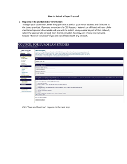


© Copyright 2026