
Solutions Manual and Reference for The Economics of Business Valuation
March 29, 2013
Solutions Manual and
Reference for The
Economics of Business
Valuation
Edited by Erin A. Grover
With Contributions from Patrick L. Anderson,
Samantha Superstine, and Jeff Johnson
Entire contents © 2013 Anderson Economic Group, LLC
Anderson Economic Group LLC
1555 Watertower Place
East Lansing, Michigan 48823
Tel: (517) 333-6984
Fax: (517) 333-7058
http://www.AndersonEconomicGroup.com
ISBN: 978-0-9890833-1-7
Table of Contents
Preface
Purpose .......................................................................................................................i
Design and Content ....................................................................................................i
Acknowledgements ..................................................................................................iii
Chapter 1: Theories of Value
Common Notions of Value ....................................................................................... 1
The Human Condition and “Winner’s Curse” in Business Valuation .................... 10
Chapter 2: The Nature of the Firm
Principal-Agent, Moral Hazard, and Other Problems ............................................. 15
Comparing U.S. Firms by Size ............................................................................... 17
Classifying Ownership of Businesses ..................................................................... 22
U.S. Firms by Corporation Type ............................................................................ 27
Firm Survival .......................................................................................................... 31
Chapter 3: Economic Theories of Value
Distinguishing Notions of Neoclassical Economics ............................................... 41
Mathematics of the Neoclassical Economics Model .............................................. 42
Chapter 4: Finance Theories of Value
Alternate Presentations of Complete-Markets Pricing Formulas ........................... 50
Alternate Derivations and Portfolio Models ........................................................... 55
Chapter 5: Traditional Theories of Value
A Note on Conventions; Discrete & Continuous Time .......................................... 65
Algorithms for Calculating Historical Growth Rates ............................................. 66
The Workhorse Net Present Value Algorithm ........................................................ 69
Expected Net Present Value ................................................................................... 71
Formulas for Annuities and Perpetuities ................................................................ 72
Income Subject to Termination Risk ...................................................................... 77
Fair Market Value and Other Elements to Consider in
Traditional Business Valuation ............................................................................... 78
Chapter 6: Applications
Extended Descriptions of Valuation Subject Companies ....................................... 87
Applications: Intermediate Results of Value Functional Examples in EBV .......... 99
Applications: Investment Decisions and Property Valuation ............................... 106
Chapter 7: End of Chapter Questions and Hints
Review Questions for Chapter 1: Modern Value Quandaries .............................. 120
Review Questions for Chapter 2: Theories of Value ............................................ 123
TOC 1
Table of Contents
Review Questions for Chapter 3: Failure of the Neoclassical Rule 125
Review Questions for Chapter 4: The Nature of the Firm 127
Review Questions for Chapter 5: The Organization and
Scale of Private Businesses ............................ 130
Review Questions for Chapter 6: Accounting for the Firm .................................. 133
Review Questions for Chapter 7: Value in Classical Economics ......................... 135
Review Questions for Chapter 8: Value in Neoclassical Economics ................... 137
Review Questions for Chapter 9: Modern Recursive Equilibrium ....................... 138
Review Questions for Chapter 10: Arbitrage-Free Pricing .................................. 141
Review Questions for Chapter 11: Portfolio Pricing Methods ............................. 144
Review Questions for Chapter 12: Real Options and Expanded
Net Present Value .......................................... 146
Review Questions for Chapter 13: Traditional Valuation Methods ..................... 148
Review Questions for Chapter 14: Practical Income Method .............................. 153
Review Questions for Chapter 15: Value Functional Theory ............................... 155
Review Questions for Chapter 16: Value Functional Applications ...................... 157
Review Questions for Chapter 17: Applications in Finance and Valuation ......... 158
Review Questions for Chapter 18: Law & Economics Applications ................... 162
Appendix A: Guide to Mathematics of Value
Random Variables, Measure Theory ....................................................................A-2
Stochastic Processes .............................................................................................A-5
Brownian Motion; Itô Processes; Geometric Brownian Motion ..........................A-7
Change of Measure .............................................................................................A-10
Expectation of Random Variables ......................................................................A-14
Statistics of Central Tendency and Variation .....................................................A-18
Moments and Other Measures ............................................................................A-20
Optimization Using Differential Calculus ..........................................................A-23
Calculus of Variations ........................................................................................A-26
Dynamic Programming .......................................................................................A-27
Utility Functions .................................................................................................A-31
Appendix B: Software for Business Valuation
Admonition: “No software is a substitute for thinking” ....................................... B-1
Special Tools Used in the The Economics of Business Valuation ........................ B-2
Rapid Recursive® Toolbox for MATLAB® ........................................................ B-4
Notes on Mathematical Software .......................................................................... B-6
Spreadsheets .......................................................................................................... B-8
Monte Carlo & Decision Tree Software ............................................................... B-9
Advice: “Business Valuation” Software ............................................................. B-10
Other Useful Software Not Considered Here ..................................................... B-12
General Disclaimers; Trademarks ...................................................................... B-13
TOC 2
Table of Contents
Appendix C: Errata
Corrections or Additions to The Economics of Business Valuation ..................... C-1
Suggestions for Book Authors and Errors ............................................................ C-2
TOC 3
Preface
A Brief Introduction
S ECTION 1.1. Purpose
The idea to create a companion volume was initially formulated due to
the original length of The Economics of Business Valuation (EBV).1
Additionally, given the novelty of the value functional method, the author
of EBV, Patrick L. Anderson, wanted to provide readers with additional
examples. Therefore, the purpose of this compilation of work is to provide
extensive material and references for scholars, readers, and practitioners
who purchase EBV.
This companion volume may also be useful to those interested in notions
of value in various fields, use of the net present value (NPV) rule, and/
or the mathematics of dynamic programming.
S ECTION 1.2. Design and Content
The design of this companion volume attempts to mirror the organization
of EBV. As you recall, EBV arranges every three chapters into a “part,”
which illustrates a shared theme throughout those chapters. In this pub1 See Patrick L. Anderson, The Economics of Business Valuation: Towards a Value Functional Approach, Stanford University Press, 2013.
© 2013 Anderson Economic Group, LLC
March 29, 2013
ii
lication, each chapter contains supplemental or related material to the
corresponding part in EBV; Chapter 1 corresponds with EBV Part I.
For example, Chapter 2 of the Solutions Manual discusses the principalagent problem in firms, as well as presents unique data on U.S. businesses.
This chapter is meant to supplement EBV’s Part II “The Nature of the
Firm.” To further illustrate this design, we named each chapter after its
counterpart in EBV.
As described in Appendix B “Guide to the Solutions Manual,” this compilation of work covers a wide range of fields. The extended material
provided here includes a discussion of the following topics:
• common notions of value (Section 1.1. on page 1)
• the “winner’s curse” and the human condition (Section 1.2. on page
10)
• principal-agent and moral hazard problems (Section 2.1. on page 15)
• business entity classifications and other forms of organization for private businesses (Section 2.3. on page 22)
• types of U.S. firms in terms of size, organization, employment, and
survival rates (Section 2.2. on page 17, Section 2.4. on page 28, and
Section 2.5. on page 32)
• neoclassical economics in the real world (Section 3.1. on page 42)
• the math behind the neoclassical model in economics (Section 3.2. on
page 43)
• complete market pricing formulas (Section 4.1. on page 51)
• applications of Mathematics to problems in Finance (Chapter 5)
• existing valuation standards (Section 5.7. on page 79)
• software for business valuation (Appendix B)
In addition to these topics, we provide several other value functional
examples and explanations that expand upon Part VI “Applications” of
EBV.2 We include a set of questions and problems for each EBV chapter,
as well as hints for several of these problems in Chapter 7. We also
provide a guide to the mathematics of value, which expands upon the
summary of notation and important formulas presented in Appendix A
“Key Formula and Notation Summary” in EBV.3 Lastly, we include a
2 See Chapter 6, “Applications: Intermediate Results of Value Functional Examples in
EBV.”
3 See Appendix A “Guide to Mathematics of Value.”
March 29, 2013
iii
section for errata and additional references, should any errors be found
or clarifications needed in EBV or this companion volume.4
S ECTION 1.3. Acknowledgements
I must acknowledge that this was most definitely a group effort and the
following individuals greatly contributed to this companion volume:
Samantha Superstine, who compiled and analyzed the business data for
Chapter 2 “The Nature of the Firm,” as well as authored the bulk of it.
She also graciously offered her time to assist in proofreading and editing
several of the other chapters.
Jeffrey Johnson, who authored Chapter 6 “Applications.” He ran the
analysis for each value functional example, as well as provided a description for each that was understandable to even the non-programmer, which
was so greatly appreciated.
Manav Garg, who graciously reviewed the math and equation heavy
content of this companion volume. He checked for accuracy and provided
comments for Chapters 4 and 5, as well as Appendix A.
Christi Lilleboe, Tyler Theile, and Kimberly Kvorka each helped in a
multitude of tasks. Christi was essential to streamlining the format of this
companion volume. She also assisted in proofreading and editing text as
well as reformatting equations using MathType. Tyler helped to ensure
that this companion volume made it on the web, as well as had an ISBN.
Kim assisted in organizing original writings and a multitude of other
administrative tasks.
Last, but certainly not least, Patrick L. Anderson, the author of The
Economics of Business Valuation, without which this companion volume
would not have made much sense. He was kind and encouraging to allow
me the opportunity to create this publication. As part of that initiative,
he provided us with the bulk of writing that constitute Chapters 1, 3, 4,
5, and 7, in addition to Appendices A and B.
4 See Appendix C “Errata.”
Chapter 1
Theories of Value
by Patrick L. Anderson
An Introduction
There are many concepts of value, just as there are many theories of value
that are valid within the confines of their defined assumptions and limitations. In this chapter, we first discuss common notions of value, and
how value is determined in various fields. This gives historical and
practical context to perceptions of value. We then describe how different
people could attribute different values to the same item, and particularly
how that differentiation applies in the case of business valuation.
S ECTION 1.1. Common Notions of Value
a. What is a “standard” of value?
Given the amorphous nature of the simple term “value,” it should not be
surprising that several different specific standards of “value” are in common use. By “standard of value,” we mean the practical definition of
value, and not the method of determining that value, nor the theoretical
basis for that practical definition.1 In this section, we discuss standards
of value that are commonly used by economists, businessmen and women,
investors, and tax authorities.
© 2013 Anderson Economic Group, LLC
1
Page 2
b. Market Value in Economics
The most critical aspect of the market, and the market price, is the
existence of competing buyers and sellers. It is this competition among
self-interested parties that makes the sales price so efficient. Indeed, much
of the triumph of capitalism around the world over the last two centuries
can be traced to the efficiency of markets, and the mechanism of market
prices.
The intellectual basis for free markets as the economic system that would
most enrich society was laid in the seminal work of Scottish moral
philosopher Adam Smith, who in 1776 penned the magisterial Wealth of
Nations. In particular, Smith identified free markets as the “invisible
hand” that allocates world resources in a manner both equitable and
encouraging of prosperity.2
The Primacy of the Market
Market value is the standard on which we will base the majority of the
analysis in this publication, and is a deeply established principle in economics. In general, the “market value” of any asset is the price at which
it exchanges among willing parties in a market; a market, in turn, consists
of multiple potential buyers and sellers, and facilitates reasonably good
information about the asset itself. The legal definition of “fair market
value” used in the United States closely matches this economic concept,
and will be described further below.
The “Free Market” and Institutions
Note that the existence of a market does not guarantee that an asset is
actually sold. Indeed, if a seller is compelled to sell, it is no longer a true
market. The lack of compulsion means that buyers and sellers can pursue
1 This concept, unfortunately, does not have a consistent name or definition among professional valuation standards. The Appraisal Foundation’s USPAP (2010) uses the term “type
or definition of value.” “Standard of value” is defined as “identification of the type of
value being used” in the ASA Business Valuation Standards (2009) glossary. The IVSC
International Valuation Standards (2010 exposure draft) uses the term “basis of value”
and defines it as “statement of the fundamental measurement assumptions of a valuation”
2 We discuss Smith and his contemporaries in EBV Chapter 7 “Value in Classical Economics.” The findings of welfare economics are discussed in EBV Chapter 8 “Value in Neoclassical Economics.”
Solutions Manual and Reference for The Economics of Business Valuation
their own interests in a true market, and justifies the use of the terms
“free market” and “free market price.”3
Furthermore, a market does not require perfect information, a lack of
transaction costs, government-sanctioned standards for the product, or
most other attributes that exist in the markets for many consumer products. A market does require, however, certain institutional factors, including property rights and the enforcement of contracts—two critical features
of society that are normally secured by government. We discuss this topic
in EBV Chapter 4 “The Nature of the Firm.”
c. The “Fair Market Value” Legal Standard
The “fair market value” concept from economics is one of the most
powerful and useful to emerge from that field. Indeed, it is now codified
in countless laws, standards, court cases, individual contracts, and scholarly treaties in the United States and in other countries.
This legal standard is essentially identical with the economic concept:
fair market value means the value in a market with willing buyers and
willing sellers, each with sufficient information, and neither under any
compulsion.4 This standard has been refined in countless court cases, IRS
rulings, and reference books.5
3 The intellectual basis for free markets as the economic system that would most enrich
society was laid in the seminal work of Scottish moral philosopher Adam Smith, who in
1776 penned the magisterial Wealth of Nations. In particular, Smith identified free markets
as the “invisible hand” that allocates world resources in a manner both equitable and
encouraging of prosperity.
4 The seminal reference for this definition is the IRS Revenue Ruling 59-60 (1959) 59-1 CB
237, which defines fair market value as:
The price at which the property would change hands between a willing buyer and a
willing seller when the former is not under any compulsion to buy and the latter is
not under any compulsion to sell, both parties having reasonable knowledge of relevant facts.
Court decisions frequently state in addition that the hypothetical buyer and seller
are assumed to be able, as well as willing, to trade and to be well informed about the
property and concerning the market for such property.”
5 For example, Treasury Regulation 20.2031-1 defines fair market value as:
“The price at which the property would change hands between a willing buyer and a
willing seller, neither being under any compulsion to buy or to sell and both having
reasonable knowledge of relevant facts.”
Page 4
We note here several specific observations about this standard:
• “Fair market value” must be set in a market, meaning multiple potential buyers and sellers. Multiple potential buyers, however, does not
mean multiple offers to buy, rather that multiple persons are interested
in purchasing similar assets and are capable of purchasing this one.
• Another implication of “market” is that the buyers and sellers are
independent of each other. This is sometimes included explicitly in the
definition of an “arm’s length” transaction. Note that “arm’s length”
does not mean the parties do not know each other, have no other
mutual business interests, or the like, but rather that decisions of
whether to buy or sell are made with individual interests in mind.
• The market must include willing parties to complete the transaction.
Transactions by non-willing sellers—such as those compelled by eminent domain decrees, or by financial distress—do not constitute a
market.
• In addition, the “sufficient information” phrase requires that market
participants have adequate information, though not perfect information. Several “sales” of the Brooklyn Bridge, for example, would not
demonstrate a market price if all the sales were to gullible “buyers” of
a worthless piece of paper.6
The market value of any specific asset is, in general, different than the
value of that asset to an individual owner. Individuals often place peculiar
emphasis on certain assets, and therefore those assets may be “worth”
more to them than their respective market values. (See the discussion of
investment value or intrinsic value, below.)
d. “Investment Value”
The term “investment value” has an important economic implication,
which we will note in discussing the value of privately-held firms and
6 References to “selling the Brooklyn Bridge” have appeared in American literature for over
a century. A few recent efforts to track the original source arrived a contradictory results.
Some authors attribute the story to the exploits of William McCloudy and George C.
Parker, who were said to have sold the bridge to recent immigrants (Parker giving the
buyer a bill of sale saying “one bridge in good condition”) around 1900. According to the
story, McCloudy was subsequently convicted of larceny in 1901. Others say even this
story is a myth, perhaps even a braggadocio among professional con men.
A skeptical but entertaining review of these stories was penned by novelist Gabriel Cohen
(2005); less skeptical accounts are from the language scholar Barry Popik (2004) and the
urban-myth-investigator web site “Straight Dope” (2007).
Solutions Manual and Reference for The Economics of Business Valuation
those without widely-traded securities. It also has related technical meanings in Finance and Accounting.
Economic Concept
In general, the term “investment value” refers to the value of an asset as
an investment, distinguishing it from the value in use for personal consumption. This distinction is important when deriving a theory of investment behavior. As discussed in EBV Chapter 8 “Value in Neoclassical
Economics,” the purpose of investment is to secure future consumption,
and not to achieve other goals.
The fallacy of ignoring this principle becomes clear when one attempts
to use standard finance techniques to explain the behavior of investors.Explaining investor behavior requires taking this principle into
account when regarding assets and other considerations they consider to
be important, such as a house, reputation, standard of living, loyalty, or
the use of time. In such matters, a person may quite rationally ignore a
“rule” of finance (such as the NPV rule) when it conflicts with personal
interests. However, the very same person may attempt to follow the very
same “rule” when dealing with an investment portfolio. Contemporary
authors in finance seem more prone to erroneously missing this distinction
than those of many decades ago; for example, both Irving Fisher and
John Burr Williams made such a distinction in their writings.7
Investment Value: International Valuation Standard
The term “investment value” also has a technical definition that is related
to the economic concept described above. The following is excerpted
from the International Valuation Standards:
Investment Value, or Worth. The value of property to a particular investor, or a class of investors, for identified investment objectives. This
subjective concept relates specific property to a specific investor, group
7 See the excerpted passages of Fisher and Williams in EBV Chapter 3 “The Failure of the
Neoclassical Investment Rule.” Note how Fisher used the term “investment opportunity”
and Williams the term “investment value.”
Not all contemporary authors ignore this distinction. For example, John Hull, in the standard reference Options, Futures, and Other Derivatives, distinguishes between “consumption assets” and “investment assets,” cautioning investors about using Finance techniques
intended for the latter for the former. See, e.g., Hull (2000, p. 50, 55).
Page 6
of investors, or entity with identifiable investment objectives and/or criteria.8
Similar definitions in common use include “the value to a specific investor, based on that investor’s requirements, tax rate, or financing,” and
“the value of an asset to its owner, depending on his or her expectations
and requirements.” These statements implicitly emphasize the distinction
between the value in the marketplace of many buyers and sellers (which
would establish the fair market value) and the “investment value” to a
particular owner.
“Fair Value”
The term “fair value” has a specific meaning when used in financial
statements created under Generally Accepted Accounting Principles
(“GAAP”) in the United States. These principles are used in reporting
financial statements for most public and private firms.9 Under the
recently-adopted statement of the body that governs GAAP accounting
principles, “fair value” is defined as follows:
Fair value is the price that would be received to sell an asset or paid to
transfer a liability in an orderly transaction between market participants
at the measurement date.10
The standard goes on to describe an “orderly transaction,” noting that it
requires some “exposure to the market” but is not a “forced” sale. It also
describes the market to be either the “principal” or “most advantaged”
market for the particular asset. “Market participants” are defined as parties
that are “independent” of the reporting entity, “knowledgeable” about the
asset, and “able” and “willing...but not forced” to complete the transaction.11
8 Excerpted from the Exposure Draft of IVS2, dated July 2006, section 3.
9 Reporting financial statements are typically not the same as those used for tax purposes,
and may not be the same as those used by management or for regulatory purposes. However, they are often the preferred set of statements for investors and managers, because
they use a consistent set of rules based on the principle of providing investors with an
accurate picture of the enterprise.
10 Financial Accounting Standards Board, Statement of Financial Accounting Standards 157
(“FAS 157”), (September 2006), paragraph 5.
11 FAS 157 (September 2006), paragraphs 7-10.
Solutions Manual and Reference for The Economics of Business Valuation
The Financial Accounting Standards Board (FASB) noted that there were
differences in the previously-used definitions of “fair value,” which
resulted in inconsistent reporting.12 It also noted that the new definition
of “fair value” adopted for reporting purposes was “generally consistent
with similar definitions of fair market value used for valuation purposes,”
citing the “fair market value” definition adopted by the Internal Revenue
Service in RR 59-60.13
“Fair Value” Under Specific State Statutes
One specific use of “fair value” arises from the use of the term in the
Uniform Business Corporation Act, and is often used in shareholder
disputes. The exact meaning of “fair value” in such cases can vary from
state to state, and be dependent on case law as well as statute.14
Intrinsic Value
The intrinsic value of an asset is its inherent or underlying worth. The
idea of “intrinsic value” in philosophy is centuries old, and means the
value “in itself” or “for its own sake.”15 This may be quite different from
the market value, which is set by competing buyers and sellers. Thus, the
notion of intrinsic value is based on the assumption that an asset can be
“worth” more to one set of persons than to another set, and even that
society as a whole can mis-estimate the value of something or someone.16
12 See FAS 157, “Summary.” The new statement replaces FAS 141, which had been the basis
for many disputes.
13 See FAS 157, paragraph C50.
14 Hitchner (2006, ch. 1) has a nice summary of this topic, along with a comparison to other
standards.
15 For example, The Stanford Encyclopedia of Philosophy quotes Plato’s dialogues (about
400 BC), Epicurius (about 300 BC), John Stuart Mill [1806-1873], and Immanuel Kant
[1724-1804] on the question of what is intrinsically good. Philosophers have sometimes
distinguished this from “extrinsic value.”
16 Contemporary philosophical debates exist, for example, on what societies should do to
protect the “intrinsic value” of human life, of other species, of specific ecosystems, and of
cultural or historical treasures.
Page 8
Intrinsic value and investment philosophy
An investor may consider a business to have intrinsic value that is not
reflected in the current market price, and therefore may decide not to sell.
Other investors may estimate the intrinsic value of stock in certain companies, and purchase stock when they consider the intrinsic value to be
higher than the market price. This is the underpinning of the “value”
approach to investment popularized by Graham & Dodd.17 The analysis
of the underlying intrinsic value is sometimes called “fundamental analysis.”18
Intrinsic value of an option
This term also has a technical meaning pertaining to financial options.
For example, a call option is a contract that gives the owner the right,
but not the obligation, to buy a security at a certain price during a certain
time period. The intrinsic value of a call option is the positive difference
(if any) between the market price and the “strike” price of the option.
Other Standards Used in Accounting and Tax
Historical Cost
The historical cost principle is a bedrock upon which accounting practice
has developed. See Chapter 6, “Accounting for the Firm.” Most assets
used in a business are put on the books at historical cost. If they are not
sold, disposed, or transferred to another party, they typically are presented
on those statements as worth the historical cost, less any accumulated
depreciation or amortization.
Historical cost is not a standard of value; it is an accounting convention.
Indeed, all accounting records, taken together, are explicitly not an indication of value—as FASB takes pains to explain:
17 Investors that pursue the philosophy of selecting companies with high underlying intrinsic
values relative to their stock prices are sometimes called “value investors.” The approach
was first popularized by Benjamin Graham and David Dodd in their 1934 book Security
Analysis, which has been reprinted and revised many times.
One famous investor that followed this advice was Warren Buffett, who received an “A+”
grade from Benjamin Graham 1951 class at Columbia University. His remembrances are
included in the 1984 article “The Superintendents of Graham-and-Doddsville.”
18 See, e.g., Reilly (1994, p. 229); Janssen (2008).
Solutions Manual and Reference for The Economics of Business Valuation
Financial accounting is not designed to measure directly the value of a
business enterprise, but the information it provides may be helpful to
those who wish to estimate its value.19
A similar pronouncement is made in the following statement from an
appraisal authority:
In this, value differs from price or cost. Price and cost refer to an
amount of money asked or actually paid for a property, and this may be
more or less than its value.20
Ubiquity of “Book Value” Term
Despite the clear statements by authorities that cost does not equal value,
“book value” is a standard term in business, tax, and finance. Unless it
happens by coincidence, most assets do not have a market value equal
to the amount shown on an accounting balance sheet as “historical cost
less accumulated depreciation.”
Perhaps fortunately, most assets do not need to be bought or sold on a
regular basis.21 Therefore, the use of book value, rather than market value,
is a useful convention.
Tax Basis
An investor that purchases equity interests in a firm has a basis in that
investment. The basis is normally equal to the cost of acquiring it.22 This
19 Financial Accounting Standards Board, Statements of Financial Accounting Concepts No.
1, 1978.
20 Henry A. Babcock, Appraisal Principles and Procedures (Washington, DC: American
Society of Appraisers, 1994), p. 95. Quoted in Hitchner (2006, ch. 1).
21 Indeed, items that are regularly purchased and used are probably not specific assets of a
business, but part of its cost of goods sold. What remains at the end of the period is typically inventory of like items.
22 In the US, the IRS defines “basis” as follows in Publication 551 (2002 edition):
The basis of stocks or bonds you buy is generally the purchase price plus any costs
of purchase, such as commissions and recording or transfer fees. If you get stocks
or bonds other than by purchase, your basis is usually determined by the fair market
value (FMV) or the previous owner's adjusted the basis of stock.
For the purposes of calculating capital gains, there may be adjustments that are necessary,
such as for depreciation.
Page 10
basis is then used to calculate gains or losses for tax purposes when the
asset is sold or transferred.
The tax basis is therefore closely associated with the accounting principle
of historical cost. It is also not, in general, equal to the fair market value
of an asset at any time after it was originally purchased.
S ECTION 1.2. The Human Condition and “Winner’s
Curse” in Business Valuation
Many mergers and acquisitions in recent decades have been proposed to
investors as value-increasing propositions. One frequently-claimed benefit was the potential for “synergies” that could result from the combination of the two organizations. So many of these failed, however, that
it has become a folk theorem that most mergers and acquisitions fail.23
Although it is probably impossible to know whether most mergers and
acquisitions fail, there is evidence to support the theorem.24
A variation of this folk theorem in mergers & acquisitions is called the
“winner’s curse.” Many mergers involve a competition among companies
desiring to acquire and control one another, and in a large share of these,
the “winner” emerges with a business that subsequently endures a reduction in market value.25
23 Ferris & Pettit (2002, chapter 2) cite unspecified articles in business publications to support this claim:
Why did more than 50 percent of the major mergers and acquisitions in the United
States completed in the 1990s, according to Business Week magazine, erode shareholder value? And why did more than 77 percent of those transactions, according to
Forbes magazine, not earn a rate of return at least equivalent to the cost of the capital necessary to finance them? The answer to both questions is often the same: overestimation of target firm value.
24 These include some rigorous research involving samples or transactions (such as Roll
[1986], who attributes much of it to “hubris”); the detailed examples of the type included
in the Ferris & Pettit book; and other examples that appear, from time to time, in the popular business press. Another possible alternative would be gathering a good sample of wellpublicized transactions involving public companies, and compare the subsequent market
returns of the stocks involved with those of appropriate market benchmarks.
Solutions Manual and Reference for The Economics of Business Valuation
How could so many highly-skilled corporate titans, investment bankers,
lawyers, business strategists, and M&A specialists make decisions that
appear to be so poor? What does this say about the human condition, or
(much less ambitiously) about valuation methodology?
Let us consider three documented reasons for such a failure, and one
additional possibility.
Three Sound Bases
Let us assume, as ample evidence suggests—but does not prove—that a
very large share of mergers and acquisitions “fail,” meaning that they
result in a lower value to stockholders than if the firms had remained
separate. There are at least three sound bases for such a phenomenon, all
documented in the economics literature and displayed in real life:
1. Auction fever
The behavior of bidders at auctions underlies the classic “winner’s
curse” hypothesis. Auction fever impels many bidders, caught up in
the excitement and the competition, to bid higher than some notion of
intrinsic worth.
Such behavior is amply documented in the literature, and commonly
on display at auctions. Indeed, in contemporary times, auctions or
similar events for such items as art, classic cars, and even antiques are
considered entertaining enough to be the subject of television programs.26
2. Hubris
The hubris of the acquirer was cited as one reason for a winner’s curse
by the economist Richard Roll (1986). Hubris—tragic pride—in the
25 The term “winner’s curse” generally applies to behavior in any auction, and refers to the
well-documented propensity of “winning” bidders to pay more than they might, in a more
sober mood, want to bid. The term first appeared in the economics literature in an analysis
of oil lease bidding by Capen, Clapp, and Campbell (1971), who worked for the Atlantic
Richfield energy firm (ARCO). Within the world of corporate M&A, the term found its
way into the subtitle of a popular merger & acquisition text: Valuation: Avoiding the Winner’s Curse [Ferris & Pettit (2002)]. See note above.
26 To be sure, this is a very low bar. However, the entertainment aspect indicates that human
emotion is driving behavior, creating a drama that captivates at least some viewers completely uninterested in the financial aspects of the auction.
Page 12
human condition was examined by many of the great ancient Greek
writers, as well as Shakespeare, Dante, and numerous others.27
The centuries have not banished it. It certainly exists in the business
world, as well as in politics, entertainment, sports, sibling rivalry, and
the local homeowner’s association.
3. The synergy trap
Organizations are not simple additions of asset values. Many mergers
and acquisitions involve synergistic elements, which may distort comparability to the subject company. In general, the whole of two organizations can be more, or less, than the sum of the two parts. This is
especially the case when the two are forcibly integrated.
Thus, mergers that promise “synergy” savings can result in costs and
performance deterioration, as well as confusion among customers and
employees, that overwhelm whatever actual savings occur.
A Modest Suggestion
It maybe unwise to deny the role that hubris plays in mergers & acquisitions, or to ignore the evidence of auction fever. Thus, there are some
anomalies in economic behavior on display.28 However, it is also unwise
to ignore the possibility that many highly-skilled financial practitioners,
with state-of-the-art models and ample computer resources and data,
simply got it wrong.
Perhaps some of their errors stem from defects in their valuation methodologies. This is certainly part of the problem: Ferris & Pettit (2002),
along with others argue that using traditional DCF tools, but doing a
better job, would have avoided at least some of these errors.29
A Deeper Critique
• There is, however, a deeper critique. Viewing companies as homogeneous entities, which can be combined and separated without damage
27 Ancient Greek literature elevated hubris to a central element of such epics as Homer’s
Iliad and Odyssey. Dante, in the Inferno, relegated sinners guilty of betrayal and pride to
the lowest level of hell. Hubris is dramatized in various Shakespeare plays including
Twelfth Night (“Be not afraid of greatness: some are born great, some achieve greatness,
and some have greatness thrust upon 'em”); Othello, Macbeth, Julius Caesar and others.
28 The field of Behavioral Finance focuses on these anomalies. Thaler (1988) is an early
examination of anomalies in auction behavior and the existence of a winner’s curse.
Solutions Manual and Reference for The Economics of Business Valuation
or benefit except to efficiencies of operation, is fundamentally wrong.
If we return to the definition of the firm stated in EBV Chapter 4 “The
Nature of the Firm,” we recognize this in the first few words: a firm is
an organization, and an organization consists of people. People, to say
the obvious, are not homogeneous. Thus, if the “whole” does not take
into account the essential attributes of the firm, how can the “parts”?
29 In particular, Ferris & Pettit (2002, chapter 2) describe a “ROE” [return on equity] model,
in which the accounting ratios that drive earnings to shareholders are modeled and forecast
into the future.
We discuss models of this type in EBV Chapter 13 “Traditional Valuation Methods” and
Chapter 14 “Practical Application of the Income Method.”
Chapter 2
The Nature of the Firm
by Samantha Superstine,
with contributions from Patrick L. Anderson
An Introduction
We discuss in The Economics of Business Valuation Chapter 4, “The
Nature of the Firm,” how the presentation of the firm in both standard
microeconomics and macroeconomics is still quite primitive. In microeconomics, firms are typically assumed to sell homogenous goods, using
a simple production function; markets clear on the profit-maximizing
criteria of one-period firms arrayed against aggregate consumer demand
in the market; workers consider their wages and available interest rates,
and adjust their consumption plans accordingly.30 Additionally, the driver
of businesses (the entrepreneur) is largely ignored in mainstream economics.31
This chapter is meant to supplement EBV Chapters 4, 5, and 6. We begin
by discussing the principal-agent and moral hazard problems in firms.
Then we use business data to compare U.S. firms by size and type of
firm. We then provide a discussion on business entities as they are classified into different types of categories based on tax filing status (C
corporations, S corporations, partnerships, etc). Lastly, we discuss
employment and establishment survival rates in the U.S.
30 We describe this more fully in EBV Chapter 8, “Value in Neoclassical Economics.”
31 The entrepreneurial component of new businesses is gaining attention in the mainstream
media and even academia. However, the role of the entrepreneur has not been extensively
studied, except for in Austrian economics. The editor recommends for the curious reader
the following: Israel Kirzner’s Competition and Entrepreneurship, Carl Menger’s Principles of Economics, Peter Klein’s The Capitalist and The Entrepreneur, and Peter Boettke’s
Living Economics: Yesterday, Today, and Tomorrow.
© 2013 Anderson Economic Group, LLC
14
March 29, 2013
Page 15
S ECTION 2.1. Principal-Agent, Moral Hazard, and Other
Problems
Unfortunately, the principal-agent problem in business (and related moral
hazard and other problems) is not solely theoretical, and has produced
tangible damage over the past century. In this subsection, we discuss two
seminal periods in which public attention was focused on these issues.
Public Concern over Principal-Agent Problems: the 1930’s
Public concern over separating the ownership of and control over business
ventures arose centuries after Adam Smith’s statement of the problem.
One influential, if alarmist, view was propounded by lawyer Adolph Berle
and economist Gardiner Means in The Modern Corporation and Private
Property. First published in 1932, it stated that the separation of ownership
and control in the modern corporation would cause many social ills. Those
that control the corporation, they wrote, can “serve their own pockets
better by profiting at the expense of the company than by making profits
for it.”32 This is an acute implication of “agency theory,” although this
phrase makes no appearance in the book, for it had not yet been propounded.33
There are two other, more subtle observations of Berle & Means that
deserve note. First, they observed the separation of property into consumption property and productive property. The latter category includes
investments: if investments are a different type of “property” than the
traditional home-and-hearth property, they contend, their owners will
behave differently toward them. Second, they contend that separating
ownership from control undermines the profit maximization principle
itself.34
32 Berle & Means (1932, chapter 6; p. 114 in the 1991 Transaction Edition).
33 The Introduction to the 1991 Transaction Edition, written by Murray Weidenbaum and
Mark Jensen, contains a balanced discussion about the contributions of the Berle and
Means in 1932, the subsequent business and regulatory events (including the disappearance of many former corporate giants, and periodic merger waves), and the later appearance of agency theory.
34 On these points, see the Introduction to the 1991 Transactions Edition, and the passages in
Book IV, Chapter 2, and Book I, chapter 6.
March 29, 2013
Solutions Manual and Reference for The Economics of Business Valuation
Recent Accounting Scandals
Decades later, public concern again arose over widespread abuse, underlining the seriousness of the principal-agent problem. Ironically, it was
the perversion of one of the measures from the 1930’s that led to this
wave of reform: the use of an “independent” accounting firm to audit the
books.
Indeed, the word “public” in the term “certified public accountant” highlights the duty to the public interest that is supposed to be served when
an independent accountant prepares or reviews accounting records. In
most cases, accounting firms play a valuable and specific role as the
independent auditor to publicly-traded firms.
Over time, however, these same firms learned they could also act as
consultants to the company. In such a role, they could earn very large
fees for advice on a range of managerial, accounting, tax, and technical
issues. The boards of directors of such companies should have identified
this conflict of interest and taken steps to prevent abuses. Unfortunately,
in some cases the fees earned from these consulting arrangements corrupted the independence of the audit function performed by the same
firm. This was clearly evidenced in scandals such as those involving
Enron Corporation, Worldcom, and others. However, the extent of the
conflicts of interest extended far beyond these firms. Tirole (2006, section
1.2) notes that, as of 2001, nonaudit fees constituted more than half of
the fees paid to accounting firms in 28 of the 30 firms comprising the
Dow Jones Industrials.
The damage from these scandals went far beyond the destruction of a
few firms and several careers. As investors became aware of the corruption of the role of “independent” auditing by accounting firms, they began
to worry about the accuracy of financial reports for publicly traded companies in general. Due to these concerns, an enormous amount of market
capitalization of publicly-traded firms evaporated. Largely as a result of
these scandals, Title II of the federal Sarbannes-Oxley Act of 2002 now
prohibits the use of auditors to perform significant consulting tasks for
the same firms.35
35 Sarbannes-Oxley Act of 2002, Title II, section 102. Of course, as in most laws there are
exceptions and other things? variables? that managers should consider before concluding
that a specific arrangement is lawful or unlawful.
March 29, 2013
Page 17
There is nothing uniquely American in this experience; a number of other
countries have experienced similar accounting scandals (though few on
the scale of those in the U.S.). As a result of these and other concerns,
many countries have adopted codes of good governance, including Brazil,
France, Russia, the UK, and Singapore.36 These codes supplement other
rules, including stock exchange rules, state and national laws, and
accounting standards.
Implications: Investor Confidence, Information, and the PrincipalAgent Problem
The passage of a law rarely solves a fundamental problem, and SarbannesOxley is no exception. The fundamental principal-agent problem still
exists with large businesses in which stockholders do not manage the
firm. Although auditor independence is now better than before, many
firms still rely on accountants to perform a range of services outside of
auditing.37 Furthermore, investors rely on information that is not the
responsibility of a firm’s accountants, such as management’s assessments
of business conditions, competitor actions, and the company’s pipeline
of new products. These statements to the investment community are
fundamentally the decisions of managers, and it is their responsibility to
ensure any ensuing statements are based on good information, whether
the statements originate from accountants, engineers, economists, financial managers, operational experts, lawyers, or public relations consultants.
S ECTION 2.2. Comparing U.S. Firms by Size
Do very large, publicly-traded firms dominate the U.S. economy (meaning that their revenues, employees, profits, and influences exceed that of
other firms)? Do they tower so high above the teeming masses of small
businesses that the American economy depends more on a handful of big
corporations than on smaller companies?
36 See Tirole (2006, section 1.3).
37 Recall that the Sarbannes-Oxley proscription only applies to firms covered by the Act,
which are largely publicly-traded firms.
March 29, 2013
Solutions Manual and Reference for The Economics of Business Valuation
We present data below, which indicate that the businesses that employ a
majority of private-sector workers, are neither large nor publicly-traded.
In particular, the data establishes that the majority of the employment
and earnings in the private sector economy of the United States come
from small and mid-sized firms, almost all of which are privately held.38
Furthermore, a significant fraction of very large firms are privately held.
a. The Role of Small and Large Firms
As stated in EBV Chapter 4 “The Nature of the Firm,” small businesses
(which we define as nonfarm entities with fewer than 500 employees)
are a significant part of the national economy. While it may be easy to
assume that large firms with recognizable names and products are responsible for the majority of the economy, small businesses account for at
least 40% of national numbers for key economic indicators.
In 2010, small businesses accounted for 49% of employment, 43% of
annual payroll figures, and 84% of establishments nationwide.39 To extend
these calculations to firms, small businesses make up 99.7% of firms
nationwide, leaving large businesses to account for only 0.3% of firms.
In other words, of the 5.7 million firms in 2010, only slightly more than
17,000 employed more than 500 workers.
Despite the ratio of small to large businesses, large and midsized firms
are responsible for most business revenue in the United States. In 2007,
large firms accounted for 62% of revenues ($18.4 trillion of approximately $29.7 trillion), with the rest coming from small and midsized
firms.40
38 The U.S. Census Bureau’s County Business Patterns (CBP) covers data on most industries, excluding crop and animal production; rail transportation; National Postal Service;
pension, health, welfare, and vacation funds; trusts, estates, and agency accounts; private
households; and public administration. More details about the data used for CBP data can
be found here: http://www.census.gov/econ/cbp/overview.htm
39 The U.S. Census Bureau distinguishes between “firms” and “establishments:” an establishment is a fixed location at which economic activity occurs, and therefore a firm may
have one or many establishments. “Businesses” may be used referring to either type of
entity. Establishment activity is defined by March employment, and excludes governmental establishments except liquor stores, wholesale liquor establishments, depository institutions, federal and federally sponsored credit agencies, and hospitals.
40 Most recent revenue data is only available every 5 years. See Table 2-1 on page 19 for
2007 business data from the U.S. Census.
March 29, 2013
Page 19
See Table 2-1 and Table 2-2 below for detailed statistics on employment,
payroll, and when applicable, revenues, by firm size. For every metric
since 2007, the large business category has had slight increases in its
contribution to national figures.
TABLE 2-1. Firm Data by Size (2007)
ENTERPRISE
EMPLOYMENT
SIZE
NUMBER
OF FIRMS
(a)
0-4
5-9
10-19
<20
20-99
100-499
<500
500+
Total
Percentage for <500
Percentage for 500+
NUMBER OF
ESTABLISHMENTS
ANNUAL
PAYROLL
($1000s)
EMPLOYMENT (b)
ESTIMATED
RECEIPTS
($1000s)
3,705,275
1,060,250
644,842
5,410,367
532,391
88,586
6,031,344
18,311
6,049,655
3,710,700
1,073,875
682,410
5,466,985
723,385
355,853
6,546,223
1,158,795
7,705,018
6,139,463
6,974,591
8,656,182
21,770,236
20,922,960
17,173,728
59,866,924
60,737,341
120,604,265
$
234,921,325
$
222,419,546
$
292,088,277
$
749,429,148
$
768,546,555
$
686,862,018
$ 2,204,837,721
$ 2,821,940,511
$ 5,026,778,232
99.7%
0.3%
85%
15%
49.6%
50.4%
44%
56%
$
$
$
$
$
$
$
$
$
1,434,680,823
1,144,930,232
1,395,498,431
3,975,109,486
3,792,920,977
3,612,050,221
11,380,080,684
18,366,661,220
29,746,741,904
38%
62%
(a) The U.S. Census Bureau distinguishes between “firms” and “establishments.” An establishment is a fixed location at which
economic activity occurs, and therefore a firm may have one or many establishments.
(b) Employment is defined by the number of employees on the payroll at the time of data collection (Mid-March pay period)
(c) Receipt data available every five years; most recent release is 2007 data.
Source: U.S. Census Bureau, 2007 County Business Patterns and 2007 Economic Census.
Analysis: Anderson Economic Group, LLC
TABLE 2-2. Firm Data by Size (2010)
ENTERPRISE
EMPLOYMENT
SIZE
0-4
5-9
10-19
<20
20-99
100-499
<500
500+
Total
Percentage for <500
Percentage for 500+
NUMBER OF
FIRMS (a)
NUMBER OF
ESTABLISHMENTS
ANNUAL
PAYROLL
($1000s) (c)
EMPLOYMENT (b)
3,575,240
968,075
617,089
5,160,404
475,125
81,773
5,717,302
17,236
5,734,538
3,582,826
982,019
652,662
5,217,507
648,386
354,313
6,220,206
1,176,422
7,396,628
5,926,452
6,358,931
8,288,385
20,573,768
18,554,372
15,868,540
54,996,680
56,973,415
111,970,095
99.7%
0.3%
84%
16%
49.1%
50.9%
$
$
$
$
$
$
$
$
$
226,541,056
212,039,611
283,246,473
721,827,140
719,061,251
665,644,629
2,106,533,020
2,834,450,349
4,940,983,369
43%
57%
(a) The U.S. Census Bureau distinguishes between “firms” and “establishments.” An establishment is a
fixed location at which economic activity occurs, and therefore a firm may have one or many
(b) Employment is defined by the number of employees on the payroll at the time of data collection (MidMarch pay period)
(c) Receipt data available every five years; most recent release is 2007 data.
Source: US Census Bureau, 2012 County Business Patterns and 2012 Economic Census.
Analysis: Anderson Economic Group, LLC
March 29, 2013
Solutions Manual and Reference for The Economics of Business Valuation
Number of Firms, Establishments, and Employees for Large
Businesses
Noting the vague boundaries between “midsized” and “large” firms, it is
difficult to neatly compare the economic significance of each. However,
by issuing a specific cutoff by which to define a boundary between
midsized and large firms, we can estimate the dominance of large corporations with a bit more precision.
Having looked at the contributions of different-sized firms to the national
economy, we can now turn to data that is specific to large business to
analyze what portion of national employment and payroll come from
businesses that are considered to be “large enterprise size.”41 We can
roughly classify firms with more than 5,000 employees as “big corporations”; firms with 5,000 or less employees can therefore be classified as
small and midsized firms. EBV Chapter 5 “The Organization and Scale
of Private Business” discusses in further detail the reasoning behind
classifying certain levels of employee size as “small,” “midsized,” or
“large.”
Table 2-3 on page 21 displays firms, establishments, and employees for
large businesses in 2007 and also offers a comparison to small and
midsized firms as a whole. Table 2-4 on page 22 shows the same data for
2010, with the exception of business receipts.42 The proportion of employment and payroll between the two time periods is very similar, with less
than a percentage point decrease in the contribution of small and midsized
firms from 2007 to 2010.
41 As stated in EBV Chapter 5, large enterprise can be defined as firms with greater than
5,000 employees.
42 Data on estimated receipts is released every five years, with the last release being for 2007
data.
March 29, 2013
Page 21
TABLE 2-3. Firm Data for Large Businesses (2007)
ENTERPRISE
EMPLOYMENT SIZE
NUMBER
OF FIRMS
< 500
500-749
750-999
1,000-1,499
1,500-1,999
2,000-2,499
2,500-4,999
<5,000
5,000-9,999
10,000+
Total
6,031,344
6,094
2,970
2,916
1,542
942
1,920
6,047,728
952
975
6,049,655
NUMBER OF
ESTABLISHMENTS
ANNUAL
PAYROLL
($1000s)
EMPLOYMENT
6,546,223
71,702
45,990
59,311
46,221
36,388
118,282
6,924,117
115,222
665,679
7,705,018
59,866,924
3,695,682
2,561,972
3,552,259
2,664,416
2,094,728
6,687,266
81,123,247
6,628,415
32,852,603
120,604,265
Share of employment, payroll, & receipts of firms
<5,000 employees
>5,000 employees
67.3%
32.7%
$
$
$
$
$
$
$
$
$
$
2,204,837,721
152,059,022
109,833,289
153,957,992
120,606,441
94,001,450
320,640,371
3,155,936,286
324,791,017
1,546,050,929
5,026,778,232
62.8%
37.2%
ESTIMATED
RECEIPTS
($1000s)
$ 11,380,080,684
$
800,475,934
$
636,199,229
$
792,993,702
$
695,739,349
$
544,038,807
$ 1,979,674,138
16,829,201,843
$ 2,263,012,551
$ 10,654,527,510
$ 29,746,741,904
56.6%
43.4%
Source: U.S. Census Bureau, 2007 County Business Patterns and 2007 Economic Census.
Analysis: Anderson Economic Group, LLC
The 2010 data show that small and midsized firms make up 67% of
private-sector employment, and 62% of private-sector payroll.43 “Big
corporations” are not responsible for the majority of national employment
and earnings in the private sector. These statistics further establish the
percentage of the nation’s workers that depend on small and midsized
firms for employment.
43 2007 data also indicate that small and midsized firms account for 57% of revenues for private-sector firms. More recent data is not available for receipts.
March 29, 2013
Solutions Manual and Reference for The Economics of Business Valuation
TABLE 2-4. Firm Data for Large Businesses (2010)
ENTERPRISE
EMPLOYMENT
SIZE
<500
500-749
750-999
1,000-1,499
1,500-1,999
2,000-2,499
2,500-4,999
<5,000
5,000-9,999
10,000+
Total
NUMBER
OF FIRMS
5,717,302
5,681
2,808
2,801
1,489
872
1,761
5,732,714
906
918
5,734,538
Share of employment & payroll
<5,000 employees
>5,000 employees
NUMBER OF
ESTABLISHMENTS
EMPLOYMENT
6,220,206
75,291
50,248
64,098
46,947
39,603
124,386
6,620,779
114,667
661,182
7,396,628
54,996,680
3,452,042
2,420,696
3,410,858
2,577,221
1,947,272
6,165,819
74,970,588
6,286,593
30,712,914
111,970,095
ANNUAL
PAYROLL
($1000s)
$
$
$
$
$
$
$
$
$
$
67.0%
33.0%
2,106,533,020
154,084,058
111,747,776
159,335,433
125,317,927
93,586,405
319,664,717
3,070,269,336
337,069,838
1,533,644,195
4,940,983,369
62.1%
37.9%
Source: U.S. Census Bureau, 2012 County Business Patterns and 2012 Economic Census
Analysis: Anderson Economic Group, LLC
S ECTION 2.3. Classifying Ownership of Businesses
The data in the previous section implies that the notion of dominant large
corporations is a myth, if you define “large corporations” as those that
are numbered on either of the Fortune 1000 or the Forbes Global 2000
lists. If these data correctly portray the U.S. economy, privately-held firms
should be identified as the mainstay of the U.S. economy.
Business entities can be classified into different types of categories based
on tax filing status, which we discuss in greater detail in Section 2.4.,
”U.S. Firms by Corporation Type” on page 28. These categories, however,
are associated with how each entity is owned. This section provides
insight into variations in types of businesses, based on the ownership of
each separate entity. Detail regarding the characteristics of publiclytraded, privately-held, or non-firm/non-business entities is shown in
Exhibit 2-1, “Characteristics of Filing Entities,” on page 27. Select types
of variations are explained below.
a. Publicly-Traded Corporation Variations
Publicly-traded companies allow for partial ownership to be acquired via
purchases and sales by the public. As depicted in Exhibit 2-1, “Charac-
March 29, 2013
Page 23
teristics of Filing Entities,”, publicly-traded companies include many C
corporations (C corps). There are other forms of public corporations that
should be considered:
1. Mutual Funds
A mutual fund, in particular a stock mutual fund, is an investment
fund that is organized by investors who purchase shares in the fund,
with the fund using those proceeds to purchase equity investments in
other publicly-traded firms, along with cash investments and other
securities. In general, we consider these to be pass-through entities,
allowing private investors to achieve some diversification and professional investment management, primarily for their investments in
publicly-traded firms. However, some mutual funds (such as “hedge
funds” and “private equity” funds) can invest in private firms.
2. Real Estate Investment Trusts (“REITs”)
These trusts invest in real estate, and allow for special tax treatment of
real estate to flow through to investors. REITs can be part of more
complicated structures, including publicly-traded companies. Taubman Centers is an example of a publicly-traded corporation whose
principal operating business is a REIT.
b. Privately-Held Variations
Privately-held corporations include some C corps, as well as most S
corporations (S corps) and partnerships. Through the centuries, there have
been an enormous variety of privately-held business organizations. We
describe in some detail the most important in terms of economic scale
and taxable activity in Exhibit 2-1, “Characteristics of Filing Entities,”
on page 27. However, there are some other variations that deserve note:
1. The profitable association
Associations often are founded for charitable, social, and benevolent
purposes. After some years, these same associations may begin to
form business entities to serve their members. In a number of cases,
these business entities have grown quite large.
Life, health, and auto insurance; retirement housing; drug purchasing;
affiliated merchandise sales; and land development are some of the
industries in which these business entities provide goods and services.
Depending on the profit motive and separate identity, these organizations may or may not constitute bona fide firms.
March 29, 2013
Solutions Manual and Reference for The Economics of Business Valuation
2. The criminal syndicate
The history of 20th-century America includes many chapters of criminal gangs, often originating in various ethnic emigrations to the
United States. A number of these grew to become business operations
that appear to meet the definition of a firm.44 However, the notion of a
separate legal identity implies that ownership interests can be purchased and are entitled to the protections of law; these conditions are
probably not met for criminal syndicates.
3. The government-sponsored enterprise
In the United States, there are a number of government-sponsored
enterprises (“GSEs”) that operate in a manner similar to a business.45
Under the federal law that initially defined them, these entities have
private stockholders or other equity owners, and a board of directors
which may be elected by private owners.46 However, they also have a
government charter and therefore benefit from implied or explicit
government guarantees, and often receive subsidies.47
There are other variations on the quasi-public organization. These
include the United States Post Office; the Tennessee Valley Authority;
and a large variety of prisoner-labor undertakings. There are also
agencies of state and federal governments that attempt to operate like
a private firm in some manner. Some of these are covered in the category listed below.
We do not consider these to be “firms” because they fail at least the
profit-motive-for-investors test. They may also fail the separate legal
identity test, because they carry an implied government guarantee.
Sometimes they operate within a government-protected market as
well.
44 They had a separate legal identity, they had a profit motive for the “investors,” and they
had replicable “business” practices.
45 A 2007 Congressional Research Service memo lists the federal GSEs as follows:
Three of the GSEs — the Federal National Mortgage Association (Fannie Mae), the Federal
Home Loan Mortgage Corporation (Freddie Mac), and the Federal Agricultural Mortgage
Corporation (Farmer Mac) — are investor owned; the others — the Federal Home Loan Bank
System and the Farm Credit System — are owned cooperatively by their borrowers.
The same memo lists technical reasons why the Financing Corporation and the Resolution
Financing Corporation should not be included, as well as stating that the former GSE known
as “Sallie Mae” changed into a private corporation in 2004.
46 Congress defined the term “government-sponsored enterprise” in the Omnibus Reconciliation Act of 1990.
47 The 2007 CRS memo reports a 2000 CBO estimate of the borrowing subsidy of specific
federal GSEs at $13.5 billion.
March 29, 2013
Page 25
4. The government-chartered enterprise
In addition to those entities that are sponsored by state or federal governments, there are also a significant number of business organizations that may have been chartered by a government at their inception,
or that receive a specific charter during their operation, but are not
fully sponsored by a government. By “charter” we mean a grant, charter, or statute that identifies a purpose, and also provides certain
authorities and benefits. Often, the benefits include exemptions from
certain taxes that private businesses must pay. These organizations,
however, are expected to compete with other businesses in at least
some markets. They may also assert that they are profit-motivated
companies, and are often organized in a similar manner. They may
generate profits, and such profits could be used to purchase other
firms.
Examples of these include some large health-care organizations such
as “Blue Cross” affiliates in some states, and certain unemployment
insurance or workers’ compensation providers. The question of
whether such an organization is fully sponsored, or merely chartered,
by the government is often a delicate one. Furthermore, the benefits
the organizations receive—notably tax exemptions—are often controversial.48
The question of whether such organizations are firms, and whether
they would have value without the special government charter,
requires careful study of the actual business, the government-provided
benefits, and any government-imposed burdens.
Imputed Earnings in Pass-Through Entities
A number of business forms result in the taxable earnings of the business
being imputed to the equity owners. These equity owners may be called
shareholders, members, partners, or some other term. If the firm’s earnings are imputed for tax purposes to the equity owners, and the firm itself
does not pay income taxes on its earnings, we call it a pass-through entity.
48 For example, many of the Blue Cross Blue Shield entities were exempt from federal taxes
for most of the 20th century, under section 510(c)4 of the Internal Revenue Code. However, Congress revoked the tax-exempt status for most “nonprofit” health insurers in 1986;
section 510(m)1 now explicitly taxes “commercial-type insurance” even if it is provided
by a nonprofit entity. Some states (such as Michigan) allow a state tax exemption to such
firms, others do not. See Sallee et al. (2007, section II).
March 29, 2013
Solutions Manual and Reference for The Economics of Business Valuation
For example, a firm that earned (under tax accounting) $100,000 in a
year would apportion those earnings to its members; a 50% equity owner
would then pay federal income tax on $50,000 in earnings. It is important
to note that the income is imputed to the members, rather than actually
paid to them. In general, the amount of taxable earnings imputed to
members is different, and often quite different, from the amount of money
actually distributed to them. Even a firm with steady earnings and capital
investments would have taxable earnings different than actual cash earnings or accounting cash flow in any given year. Furthermore, most growing firms must have a portion of their earnings retained in the firm for
“working capital” purposes. We discuss this important, and often overlooked, factor in EBV’s Chapter 14 “Practical Application of the Income
Method.”
Exhibit 2-1.
Characteristics of Filing Entities
March 29, 2013
Type of Entity, by Tax Filing Status (a)
Ownership
Non-firm or non-business entity
Privately-held firms
Publicly-held firms
Corporation Filers
C Corporations (1120)
relatively few with operating income
most small and medium
corporations; some large
S Corporations (1120S)
relatively few with operating income
almost all
Investment trusts: REITs, RICs (1120-REIT,
1120-RIC)
pass-through entities for real estate and
investment earnings
many, though with large number
of shareholders
many, though with large number of
shareholders
some; excluded from
"nonfinancial" firms
some; excluded from "nonfinancial"
firms
Financial Insitutions (Banks, Insurance
Companies)
most large; almost all very large
Partnerships (b)
Limited and General (1065)
relatively few with operating income
almost all
LLCs (1065)
relatively few with operating income
almost all
most have substantial wage and salary
share of revenue; many SP filers are
contract workers
all privately-held by one filer;
some fraction are actual firms.
Sole Proprietorships
Sole proprietorships (Schedule C)
Farms and Financial Institutions
Self-employed farmers (Schedule F); Other
Agricultural, Fishery, Timber
Financial Institutions (banks, thrifts, CUs,
insurance companies)
some portion, though farms are
almost all, but excluded from most
excluded from most "business" statistics "business" statistics
relatively few with operating income
some, though excluded from most
business value estimates
some, though partially excluded
from most business value estimates
intended as passive investment vehicle
some
some
most
some, as membership associations,
mutual associations, etc.
Nonprofit organizations (Form 990)
most, though may have business
affiliates
almost all privately organized
some have public charter
Tax-exempt financial and insurance
institutions (e.g. Credit Unions, nonprofit
health insurers)
some
some
some have public charter
Charities, Churches, Schools
most, though may have business
affiliates
almost all privately organized
Informal businesses
most; may or may not report taxable
business activity
some, though not filing as a
business
Criminal syndicates
some mixture of criminal, informal,
wage and salary, and business activity
all
State and Local Governments
most activities are transfer payments,
defense, or administration
Government Sponsored Entities
Operate like a firm, but without full
discipline of market or investors
Other
Mutual funds holding corporate equties
Cooperative entities (1120C), Mutual
associations
have public charter
May operate as if government
sponsor is shareholder
may have public charter
(a) Tax forms listed are based on author's analysis of common filing requirement for category. Actual filing requirements will vary by entity, year, and with changes in
tax laws.
(b) Some Partnerships file as S Corporations
Source: Categorization by Author; tax filing information, IRS.
Analysis: Anderson Economic Group, LLC
March 29, 2013
Solutions Manual and Reference for The Economics of Business Valuation
S ECTION 2.4. U.S. Firms by Corporation Type
Exhibit 2-1, “Characteristics of Filing Entities,” on the previous page
explains the tendency of various types of corporations to be publiclyowned, privately-held, or non-business entities. The following section
delves deeper into these different types of corporations, first establishing
the difference between employer and non-employer firms, and then looking to data sources to assess the contributions these corporations make
on the national business economy.
a. Number of Business Entities by Corporation Type
Most data make a distinction between employer and non-employer firms.
As discussed in EBV Chapter 5 “The Organization and Scale of Private
Business,” employer firms have at least one employee during the year,
whereas some tax-paying entities have no paid employees.
The data from the Small Business Administration (SBA) indicate that
there are nearly 29 million establishments in 2008, 5.9 million of which
had employees.49 For comparison, IRS data show “business” tax returns
filed to be almost 32 million. This is consistent with the theory that
companies may file more than one return for business dealings, which is
also explained in EBV Chapter 5.
The data also show the number of returns filed by different corporation
types. As shown in Table 2-2 on page 29, the number of returns filed by
C corps, S corps, and partnerships far exceeds the number of firms
reported by the U.S. Census Bureau. The total number of filings in 2008
from S corps, C corps, partnerships, and sole proprietorship totals 22.6
million.
Table 2-2 on page 29 displays the reported number of business entities
in the U.S., as recorded by several different agencies. Note that the
number of firms reported by the SBA is not equal to IRS filings, and that
these figures also do not perfectly respond to data presented by the U.S.
Census Bureau.
49 SBA refers to employer firms as well as establishments, listing 5.93 million firms and 7.6
million establishments in 2008. Non-employers were listed at 21.4 million, and selfemployment at 10.1 million.
March 29, 2013
Solutions Manual and Reference for The Economics of Business Valuation
TABLE 2-2. Reported Number of Business Entities in the U.S.
Small Business Administration Data
Employer Firms
Self-employment (nonincorporated)
Sum of Firms
Establishments (a)
Non-employers
Employers
Total number of establishments
millions
2008
5.93
10.08
16.01
21.35
7.60
28.95
IRS Data
C Corporation Returns Filed
S Corporation Returns Filed
Partnership Returns Filed
LLCs
Other (REIT)
Non-Farm Sole Proprietorship Returns Filed in
Sum of “Business” Tax Returns Filed in 2002
millions
County Business Patterns Data (b)
Number of Firms
Number of Establishments
Payroll (millions)
Payroll: 500+ employees
Share of payroll from firms with 500+ employees
millions
2008
1.78
4.05
3.15
1.90
0.02
22.61
31.61
$
$
2008
5.93
7.60
5,130,509
2,901,341
56.6%
(a) The SBA defines a "firm" as "an aggregation of all establishments (locations with payroll in any
quarter) owned by a parent company."
(b) CBP data are not directly comparable with IRS or SBA data
Source: U.S. Small Business Administration, Office of Advocacy; U.S. Census Bureau; U.S. Department of
the Treasury, Internal Revenue Service, SOI Bulletin.
Analysis: Anderson Economic Group, LLC
b. Estimated Taxable Business Earnings of U.S.
Corporations, Partnerships, and Sole
Proprietorships50
IRS data breaks down business returns by corporation type. For 2008 data,
• Total business net earnings for 2008 were about $1.8 trillion, on $30.4
trillion in business receipts;
50 EBV Chapter 5 “The Organization and Scale of Private Business” details the definitions
for different types of corporations, namely public and private companies, which further
consist of C corps, S corps, Limited Liability Companies (LLC), Partnerships, and Sole
Proprietorships. Furthermore, Exhibit 2-1, “Characteristics of Filing Entities,” on page 27
details characteristics of different types of filing entities by their propensity to be public,
private, or other.
March 29, 2013
Solutions Manual and Reference for The Economics of Business Valuation
• Even though C corps had the largest amount if business receipts, partnerships accounted for the highest net income of all entity types, at
$458 billion; and
• Sole proprietorships accounted for the least net income, at $265 billion.
Table 2-3 details the business receipts and net income by corporation type
for 2003 and 2008. The only values to decrease between 2003 and 2008
are net income reported for C corps and sole proprietorships, which
declined by 27% and 1.9%, respectively, over the five-year period.
Related to that, the deficit reported by C corps, when adjusted for inflation, increased by 81% between 2003 and 2008, from $380 billion to
$690 billion.
All other values saw increases, with the changes being relatively larger
for business receipts for every corporation type other than S corps, in
which case the percentage change in net income was slightly higher. Sole
proprietorships saw the smallest increases over the period of analysis,
increasing business receipts by 7.2% and decreasing net income by 1.9%.
TABLE 2-3. Business Receipts and Net Income by Corporation Type
(billions, 2008 dollars)
2003
Entity Type
2008
Business
Net
Receipts Income (c)
Change
Business
Receipts
Net
Income
Business
Receipts
Net
Income
C corps
S corps
Partnerships (a)
Sole Proprietorships (b)
REIT/RIC
$16,512
$4,859
$2,979
$1,229
$0
$533
$250
$353
$269
$179
$18,705
$6,013
$4,344
$1,317
$0
$389
$317
$458
$265
$356
13.3%
23.8%
45.8%
7.2%
0.0%
-27.1%
26.8%
29.9%
-1.8%
98.6%
Total
$25,579
$1,584
$30,379
$1,784
18.8%
12.6%
(a) Partnerships includes general, limited, and LLCs
(b) Nonfarm
(c) Net income less deficit
Source: U.S. Department of the Treasury, Internal Revenue Service, SOI Bulletin
Analysis: Anderson Economic Group, LLC
As indicated above, C corps had the most business receipts, while partnerships generated the highest amount of net income in 2008. Some of
these firms are publicly held, and some are privately owned. From this
basis, using some professional judgment, we can allocate earnings among
privately-held and publicly-traded firms, as well as allocate earnings that
we categorize implicitly as wage and salary earnings reported on business
March 29, 2013
Solutions Manual and Reference for The Economics of Business Valuation
tax returns. Furthermore, we can note that corporation types such as REIT/
RIC are classified as non-business entities, reporting no business receipts
to the IRS.
Table 2-4 shows estimates of taxable earnings for entity type, differentiating between net income contributed by private and public firms, as well
as non-business entities. These estimates indicate that more than half
(55%) of net income is generated by privately-held firms, and only 15%
by publicly-held firms.
TABLE 2-4. Estimated Taxable Earnings of U.S. Filing Business Entities
(thousands, 2008 dollars)
Reported
Business
Receipts
Type of Organization
C corps
$
non-business
public
private
18,704,829
Reported Net
Income (a)
$
Nonbusiness
Publiclyheld
Privatelyheld
388,740
0%
70%
30%
S corps
Estimated Net Income by Type of
Organization (b)
$
$ 272,118
$ 116,622
$
6,013,292
$
317,091
non-business
0%
public
0%
private 100%
$
$
$ 317,091
REIT/RIC (c)
non-business 100%
public
0%
private
0%
$
Partnerships (d)
non-business
0%
public
0%
private 100%
$
Sole Proprietorships (e)
non-business
public
private
Total
$
-
$
355,576
$ 355,576
$
$
4,343,871
$
-
458,185
$
$
$ 458,185
1,317,443
$
264,508
65%
0%
35%
$ 171,930
$
$
30,379,436
Share of total net income
$
1,784,100
-
$ 527,507
$ 272,118
$ 92,578
$ 984,476
30%
15%
55%
(a) Net income less deficit
(b) Estimates of apportionment to public/private organizations for C corps and Sole Proprietorships based on professional
judgment
(c) Although REIT/RIC corporations may be publicly-owed or privately-held, transactions are considered to be nonbusiness
(d) Partnerships includes general, limited, and LLCs
(e) Nonfarm
Source: Internal Revenue Service, SOI Bulletin
Analysis: Anderson Economic Group, LLC
March 29, 2013
Solutions Manual and Reference for The Economics of Business Valuation
S ECTION 2.5. Firm Survival
Businesses are constantly entering and exiting the economy. Now that
we have looked at businesses broken down by corporation and ownership
type, we can reaggregate data to gain insight into patterns of firm survival
rates. Survival rates are influenced by many factors and firm characteristics. Starts, closures, and bankruptcies of businesses directly impact the
total number of firms in business.
a. Births, Deaths, and Bankruptcies of Employer Firms
The Small Business Administration (SBA) dynamic business data compiles information on the number of “births” and “deaths” per year for
U.S. businesses. The SBA defines firm births as new, original establishments, which were not open in the previous year,51 and firm deaths as
closed original establishments for that year. For the earlier part of the
decade (with the exception of 2002), births outnumbered deaths. By 2008,
however, the net new number of firms (the number of births minus the
number of deaths) was negative: in 2003, net new firms totaled almost
72,000; by 2010, the net loss was close to 60,000 firms.52
These figures are reliant on several key factors about when a business is
technically “born” or “dead.” When an entrepreneur formally registers
may vary from business to business, and the death of a firm also depends
on when a business actually winds down its affairs with the proper
government entity. EBV Chapter 5, “The Organization and Scale of
Private Business” elaborates on these factors, and concludes that it is
possible that the data exaggerate the number of firms operating over the
course of a calendar year.
See Figure 2-1 on page 33 for firm births, deaths, and bankruptcies for
2000-2010. The only years that estimate a positive net change in the
number of employer firms when considering births and deaths was 2006
and 2007. The lowest net change in firms as well as the greatest number
of bankruptcies was in 2009, at 162,216 and 60,837, respectively. 2010
51 Data refers to “openings” as businesses not open in the previous quarter, whereas “births”
are the previous year. Similarly, “closings” refers to businesses that closed in the previous
quarter, and “deaths” in the year.
52 Data from Small Business Administration Firm Size Data; U.S. Dynamic Data
March 29, 2013
Solutions Manual and Reference for The Economics of Business Valuation
data still indicate a negative net change in the number of firms, although
the net loss declined to just under 60,000.
FIGURE 2-1. Births and Deaths of Employer Firms (2000-2010)53
Births and Closures
Births
Deaths
Bankruptcies
800,000
700,000
600,000
500,000
400,000
300,000
200,000
100,000
-
100,000
90,000
80,000
70,000
60,000
50,000
40,000
30,000
20,000
10,000
0
2001
2002
2003
2004
2005
2006
2007
2008
2009
2010
Source: U.S. Small Business Administration, United States Courts
Analysis: Anderson Economic Group, LLC
It is also interesting to look at the proportion of births and deaths by firm
size. In 2010, of the 534,000 firm births, over 96% had beginning employment sizes of less than 20. In the same year, only 106 firms with more
than 500 employees started, and 150 closed. These trends are fairly
consistent throughout the years, as displayed in Table 2-5 on page 34.
The amount of large firm births and deaths has decreased over time, but
their percentages of total starts and closures did not see significant
changes, due to the small proportion of large firms in these categories.
This helps to illustrate that many firms are small, and furthermore, the
majority of new firms are small, or at least start out small.
53 Note: Data presented is from March-March for one year, and excludes establishments with
no first-quarter employment. New firm births are classified by first-quarter employment
size. Methodology from 2008 forward defines births/deaths as establishment births/deaths
for single-location firms. Previously-displayed data on starts and closures of employer
firms exhibit different trends, as the values were taken from a different data source. Figures from alternate source reported earlier in EBV Chapter 5 “The Organization and Scale
of Private Business”: http://www.sba.gov/sites/default/files/sbfaq.pdf
March 29, 2013
Solutions Manual and Reference for The Economics of Business Valuation
TABLE 2-5. Births and Deaths of Employer Firms by Size (2000-2010)
Period
Total
Beginning year employment
size of firm
<20
2009-2010
2008-2009
2007-2008
2006-2007
2005-2006
2004-2005
2003-2004
2002-2003
2001-2002
2000-2001
<500
500+
Size Class as
Percent of
<20
<500
Firm births
533,945
514,426
533,839
106
96.3
99.98
Firm deaths
593,347
572,941
593,197
150
96.6
99.97
Net change
(59,402)
(58,515)
(59,358)
(44)
Firm births
518,500
497,518
518,382
118
96.0
99.98
Firm deaths
680,716
655,858
680,516
200
96.3
99.97
Net change
(162,216)
(158,340)
(162,134)
(82)
Firm births
597,074
570,251
596,843
231
95.5
99.96
Firm deaths
641,400
613,794
641,158
242
95.7
99.96
Net change
(44,326)
(43,543)
(44,315)
(11)
Firm births
668,395
639,110
668,177
218
95.6
99.97
Firm deaths
592,410
564,345
592,148
262
95.3
99.96
Net change
75,985
74,765
76,029
(44)
Firm births
670,058
640,710
669,841
217
95.6
99.97
Firm deaths
599,333
573,302
599,078
255
95.7
99.96
Net change
70,725
67,408
70,763
(38)
Firm births
644,122
616,019
643,850
272
95.6
99.96
Firm deaths
565,745
539,061
565,482
263
95.3
99.95
Net change
78,377
76,958
78,368
9
Firm births
628,917
601,927
628,655
262
95.7
99.96
Firm deaths
541,047
515,031
540,746
301
95.2
99.94
Net change
87,870
86,896
87,909
(39)
Firm births
612,296
585,552
611,976
320
95.6
99.95
Firm deaths
540,658
514,565
540,328
330
95.2
99.94
Net change
71,638
70,987
71,648
Firm births
569,750
541,516
568,280
1,470
95.0
99.74
Firm deaths
586,890
557,133
586,535
355
94.9
99.94
Net change
(17,140)
(15,617)
(18,255)
(10)
1,115
Firm births
585,140
558,037
584,837
303
95.4
99.95
Firm deaths
553,291
523,960
552,839
452
94.7
99.92
Net change
31,849
34,077
31,998
(149)
Source: U.S. Small Business Administration, Firm Size Data: U.S. Dynamic Data
Analysis: Anderson Economic Group, LLC
b. Establishment Entry and Job Creation
Data presented by the Business Dynamic Statistics (BDS) display a great
deal of information pertaining to firm and establishment entry, exit, job
creation, and job death by firm size. By definition, an establishment is a
fixed location at which economic activity occurs, and a firm may have
one or many establishments, compiled based on an aggregation of all
March 29, 2013
Solutions Manual and Reference for The Economics of Business Valuation
establishments under common ownership by a corporate parent.54 Therefore, in some cases, an establishment may also be a firm, but the number
of establishments outnumbers firms. In this section, the term “businesses”
refers to establishments.
The entry rate for any given year, as reported by BDS, is determined by
the number of establishments that enter in a year divided by the number
of firms that existed at the beginning of that year. An establishment entry
is an establishment with positive employment in the current year that has
no employment in the previous year. BDS also reports these by establishment age. In aggregate, the entry rate for new businesses has declined
from the mid-2000's, when it was fairly steady around 12%. Between
2008 and 2010, the entry rate decreased to about 9-10%; 2009 marks the
lowest entry rate (9%) since 1977, the first year in which data were
collected.
Entry and job-creation rates by all establishments followed similar growth
patterns between 2000 and 2010, with job-creation rates being steadily
higher throughout the entire decade. Job creation is defined as the sum
of all employment gains from new or expanding establishments. In 2000,
the job-creation rate was as high as 17.4% for firms of all ages and sizes,
even though net job creation that year was only 3.2%. In comparison, the
job-creation rate in 2010 was lower, at 12.4%, with a net job-creation
rate of -1.6%. The net loss of jobs in 2009 is consistent with the impacts
felt by the recession.
Despite this, however, the job-creation rate has been consistently higher
than establishment entry rates, though they have followed similar patterns
over the past decade. Figure 2-2 on page 36 shows establishment entry
and job-creation rates between 2000 and 2010. Establishment entry and
job creation tend to increase and decrease over similar time periods, but
job-creation rate is consistently higher than establishment entry rate.
54 BDS data provided by the U.S. Census Bureau. More detailed definitions can be found
here: http://www.census.gov/ces/dataproducts/bds/overview.html
March 29, 2013
Solutions Manual and Reference for The Economics of Business Valuation
FIGURE 2-2. Job Creation and Entry Rate, All Firms (2000-2010)
2010
20%
15%
10%
Entry Rate
5%
Job Creation Rate
0%
2000
2001
2002
2003
2004
2005
2006
2007
2008
2009
2010
Source: U.S. Census Bureau, Business Dynamic Statistics
Analysis: Anderson Economic Group, LLC
The job-creation rate above, does not take into consideration job destruction (losses) that occur, solely new jobs that are created by employer
firms. Job destruction is the sum of employment losses from firms contracting or shutting down. If job creation exceeds job losses, then net job
creation is positive; conversely, if job losses in a given year exceed job
creation, then there are fewer jobs in the economy.
The net job-creation rate takes these factors into account. So while the
job-creation rate will always be positive (as long as there are new hires),
the net job-creation rate may be negative (if the loss of jobs is greater
than jobs created).
Table 2-6 on page 37 shows the job-creation rate as well as net jobcreation rate by all employer firms. Until recently, the net job-creation
rate has been mostly positive over the past decade. Net creation began
to decline in 2008, and was negative in 2009 and 2010. This negative net
job-creation rate also corresponds with the lowest percentage of job
creation in the past decade.
March 29, 2013
Solutions Manual and Reference for The Economics of Business Valuation
TABLE 2-6. Job-Creation Rate and Net Job-Creation Rate (2000-2010)
Year
2000
2001
2002
2003
2004
2005
2006
2007
2008
2009
2010
Employment
Job
Creation
Job Creation
Rate
Job
Destruction
Net New
Jobs
Net Job
Creation Rate
112,624,578
114,349,928
112,123,658
112,720,031
114,002,476
115,520,908
118,921,120
119,913,219
120,083,048
113,900,772
111,175,010
19,312,020
18,452,856
19,120,170
18,267,626
17,740,729
17,880,684
19,138,681
19,425,583
17,419,510
13,797,846
13,875,971
17.40%
16.20%
16.90%
16.30%
15.70%
15.60%
16.40%
16.30%
14.60%
11.80%
12.40%
15,722,124
17,619,886
20,880,990
16,154,168
15,538,964
15,712,643
15,131,184
18,061,881
16,556,064
19,495,945
15,684,489
3,589,896
832,970
-1,760,820
2,113,458
2,201,765
2,168,041
4,007,497
1,363,702
863,446
-5,698,099
-1,808,518
3.20%
0.70%
-1.60%
1.90%
1.90%
1.90%
3.50%
1.10%
0.80%
-4.90%
-1.60%
Source: U.S. Census Bureau, Business Dynamic Statistics
Analysis: Anderson Economic Group, LLC
Similarly, the numbers presented for establishment entry rate do not take
into account establishments that have exited the industry. Establishment
exits are establishments that report zero employment for the year, when
there was some employment in the previous year. Similar to net job
creation, net establishment entry rates decline significantly when taking
establishment exits into account. 2009 did have the smallest value for
entry rates and net entry rates, with both rates being the lowest for the
decade (9.1% and -2.9%, respectively). Table 2-7 shows establishment
entries and exits for the decade, as well as entry and net entry rates.
Similar to net new jobs, the net number of new establishments was the
smallest in 2009, in the midst of the most recent recession.
TABLE 2-7. Establishment Entry Rate and Net Entry Rate (2000-2010)
Year
2000
2001
2002
2003
2004
2005
2006
2007
2008
2009
2010
Establishments
Establishment Entry
Establishment Entry
Rate
Establishment Exits
Net New
Establishments
Net Establishment Entry
Rate
6,219,280
6,348,830
6,399,351
6,460,594
6,542,356
6,679,753
6,781,915
6,888,393
6,862,476
6,678,469
6,619,139
706,598
729,529
817,867
780,414
770,133
811,533
831,706
819,510
713,069
610,082
668,861
11.36%
11.49%
12.78%
12.08%
11.77%
12.15%
12.26%
11.90%
10.39%
9.14%
10.10%
662,727
691,775
757,824
608,946
624,933
621,169
679,159
713,598
704,812
805,721
690,504
43,871
37,754
60,043
171,468
145,200
190,364
152,547
105,912
8,257
-195,639
-21,643
0.71%
0.59%
0.94%
2.65%
2.22%
2.85%
2.25%
1.54%
0.12%
-2.93%
-0.33%
Source: U.S. Census Bureau, Business Dynamic Statistics
Analysis: Anderson Economic Group, LLC
March 29, 2013
Solutions Manual and Reference for The Economics of Business Valuation
c. Survival and Employment by Entity Age
Entering the market and attracting employees are only the first steps for
business entities. Firms and establishments must also survive within their
industries and retain employment. The survival rate of a business is
dependent on many factors.
Survival and Employment by Age of Establishment
The age of an establishment itself, and not the firm that owns it, is
associated with many different characteristics, including entry and exits.
In general, trends indicate that establishments that are older have a higher
survival rate, as defined by the amount of businesses that have not exited
for a given year: the annual survival rate for establishments aged 26 or
older has been around 95% since 2002. In contrast, establishments that
are between zero and five years is much lower, ranging between 83%
and 88% in the past decade. Figure 2-3 below details establishmentsurvival-rate trends over the past decade.
FIGURE 2-3. Establishment Survival Rate by Age (2000-2010)55
100%
Establishment
Age (Years)
95%
0-5
6-10
90%
11-15
16-20
85%
21-25
26+
80%
75%
2000
2001
2002
2003
2004
2005
2006
2007
2008
2009
2010
Note: Data began being collected in 1977, therefore data on establishments aged 26+ is only available
from 2003 onwards
Source: U.S. Census Bureau, Business Dynamic Statistics
Analysis: Anderson Economic Group, LLC
The trends for establishments of all ages follow similar patterns in terms
of periods of economic growth and decline. For all businesses, the average
survival rate has been approximately 90% for the past decade. One particular note of interest is that younger businesses seem to have been the
55 Survival rates are shown based on age of the establishment itself, and not the firm by
which it is owned.
March 29, 2013
Solutions Manual and Reference for The Economics of Business Valuation
hardest-hit by the economic recession in 2009. The difference in percentage points for survival between 2008 and 2009 perfectly corresponds to
establishment age groups, with the youngest experiencing the greatest
decline at 2.8 percentage points, and the oldest experiencing the least
decline over the previous year, at 0.7 percentage points.
Another interesting variable to consider is the proportion of national
employment contributed to by businesses of varying age groups. Despite
having lower survival rates, younger businesses (aged 0-5) have the
largest employment contribution of any age group. In the past several
years, younger establishments have contributed slightly less to national
employment (with the exception of 2010), although they have consistently
provided over a quarter of national employment. Figure 2-4 on page 39
below displays the proportion of national employment by each age group
since 2000, showing that younger businesses consistently have contributed the largest proportion of employment since 2000.
FIGURE 2-4. Proportion of National Employment by Establishment
Age (2000-2010)
Firm Age (Years)
0-5
100%
90%
80%
70%
60%
50%
40%
30%
20%
10%
0%
50%
6-10
11-15
16-20
21-25
26+
Left Censored
50%
49%
48%
47%
46%
45%
45%
45%
45%
44%
9%
3%
7%
5%
7%
6%
7%
7%
8%
9%
10%
11%
13%
8%
8%
8%
8%
6%
7%
8%
9%
9%
9%
9%
9%
8%
10%
9%
8%
9%
8%
8%
8%
7%
7%
7%
7%
7%
6%
8%
9%
9%
9%
8%
9%
10%
10%
10%
9%
9%
9%
9%
16%
15%
15%
15%
15%
14%
14%
14%
13%
13%
12%
2000
2001
2002
2003
2004
2005
2006
2007
2008
2009
2010
Note: Data on firms began being collected in 1977, therefore data on establishments associated with firms aged 26+ is only available
from 2003 onwards; left censored indicates born prior to 1976 and birth year is unknown
Source: U.S. Census Bureau, Business Dynamic Statistics
Analysis: Anderson Economic Group, LLC
Survival and Employment by Age of Firm
Firms, as stated earlier, may have one or many establishments. The
following subsection presents data on establishments based on the age of
the firm that owns them. Looking at establishments by firm age presents
the data from a different view. In general, similar trends hold as the ones
March 29, 2013
Solutions Manual and Reference for The Economics of Business Valuation
that emerge when comparing establishment survival rate by age: establishments owned by older firms have a higher survival rate.
In particular, however, establishments that are associated with younger
firms have a lower survival rate than when looking at young establishments, regardless of firm age; survival rate for establishments for firms
aged zero to five was 82.6% in 2010, the lowest of all of the age groups.
For comparison, recent survival rate for establishments for firms aged at
least 26 is almost 95%. Figure 2-5 indicates survival rates for establishments based on firm ages, highlighting the tendency for older firms to
have a higher proportion of establishment survival.
FIGURE 2-5. Establishment Survival Rate by Firm Age (2000-2010)
100%
Firm Age
(Years)
95%
0-5
90%
6-10
11-15
85%
16-20
80%
21-25
75%
26+
70%
2000 2001 2002 2003 2004 2005 2006 2007 2008 2009 2010
Note: Data began being collected in 1977, therefore data on establishments associated with
firms aged 26+ is only available from 2003 onwards
Source: U.S. Census Bureau, Business Dynamic Statistics
Analysis: Anderson Economic Group, LLC
Analyzing employment data for establishments based on firm age can
also present interesting information. Establishments for older firms (particularly with an unknown birth year prior to 1976), represent nearly half
of national employment. This proportion is far larger than the amount of
employment represented by older establishments. The explanation for
this variation is that older firms may be opening new establishments
throughout the years; taking firm age into account indicates that older
businesses have a higher share of the workforce. Figure 2-6 shows the
contribution to employment by firms of different ages, highlighting the
significance of older firms.
March 29, 2013
Solutions Manual and Reference for The Economics of Business Valuation
FIGURE 2-6. Proportion of National Employment by Firm Age (2000-10)
Firm Age (Years)
0-5
100%
90%
80%
70%
60%
50%
40%
30%
20%
10%
0%
6-10
11-15
16-20
21-25
26+
Left Censored
50%
50%
49%
48%
47%
46%
45%
45%
45%
45%
44%
6%
7%
9%
3%
7%
5%
7%
7%
8%
9%
10%
11%
13%
8%
6%
7%
9%
9%
8%
9%
9%
9%
8%
8%
9%
9%
8%
8%
8%
7%
8%
10%
8%
8%
7%
7%
7%
7%
6%
8%
9%
9%
9%
8%
9%
10%
10%
10%
9%
9%
9%
9%
16%
15%
15%
15%
15%
14%
14%
14%
13%
13%
12%
2000
2001
2002
2003
2004
2005
2006
2007
2008
2009
2010
Note: Data on firms began being collected in 1977, therefore data on establishments associated with firms aged 26+ is only available
from 2003 onwards; left censored indicates born prior to 1976 and birth year is unknown
Source: U.S. Census Bureau, Business Dynamic Statistics
Analysis: Anderson Economic Group, LLC
There are many different ways to analyze data by firm characteristics.
We can break down firms by size, ownership, corporation type, and age,
among many other distinguishing characteristics. Analyzing the available
data helps to highlight the importance of smaller, privately-held firms,
that greatly contribute to the nation’s economy as a whole. There is also
an inherent degree of correlation between ownership, firm type, and size.
The combination of these factors provides meaningful insight into which
firms and establishments contribute to employment, earnings, and other
national economic factors. With the recent explosion of corporations
involved in industries such as technology, it will be interesting to observe
the contributions of younger firms to national employment in the years
to come.
Chapter 3
Economic Theories of Value
Revision History: Corrected, clarified, and reorganized, August 21. Matches AppC-Finance
Word document with MathType equations.
by Patrick L. Anderson
An Introduction
The neo-classical model of economics suggests that without interference
the market will efficiently allocate resources, goods, and services. Furthermore, this basic theory is the basis for the modern concept of value:
prices are set when supply equals demand. In this chapter, we discuss
differing notions of neoclassical economics, as well as walk the reader
through the mathematics of this model.
S ECTION 3.1. Distinguishing Notions of Neoclassical
Economics
In EBV Chapter 8 “Value in Neoclassical Economics,” the author concludes that the neoclassical theory is not a sound basis for determining
the market value of a privately-held firm because no such firm actually
fits into the neoclassical model. There is only one pervasive example in
business of true one-period profit maximization that is easily identified.
This is behavior we prohibit by law: criminal business activity.
Many persons could, with relatively little risk, increase the money they
have by turning to crime. Why don’t they? The major reason (we would
hope) is that they find it immoral to do so. Another reason is that the
risks and penalties are too great when compared to the payout. If we boil
it down to just risk and reward in a short time frame, crime does pay. If
what you truly care about is “profit maximization,” crime beats honest
work. Even criminals know this.
© 2013 Anderson Economic Group, LLC
42
March 29, 2013
Page 43
A very clear explanation of this dynamic was provided by former street
criminal, and current rap music artist, “Ice T,” in an interview reprinted
in the Guardian (UK):56
Ice T: When I got to high school, I started seeing people with things that
were beyond their means. I saw guys in the 12th grade that got cars and
you're looking at everybody asking yourself what was really going on.
Then my boys started to sell weed. They would buy pounds of homegrown weed, then sell joints for a dollar. Then my other friend, his sister used to steal the lunch ticket roll from the school and sell the tickets.
She was making a lot of money. She put us to work. She said, “You
guys sell them and I'll give you half the money.” I was like, “This little
broad is running an organised crime ring.”
When you get into that you start to hang around with people who take
pride in beating the system. That's the scary part. Everyone around you
says, “If you ain't a hustler then you're not cool.” You believe stolen
money is good, and working money is not.
Why should entrepreneurs be considered any more or less insightful,
moral, or enterprising than potential criminals? They shouldn’t; it is the
“profit maximization” model that needs to change. One-period profit
maximization in business is a road to disaster, and a road that entrepreneurs by and large do not travel. However, there are several aspects of
neoclassical economics that are useful in framing our thoughts about
value, e.g. price is determined by supply and demand. Below we describe
the math behind the neoclassical model, which serves as the foundation
of microeconomics; in particular, we focus on consumer preferences and
utility, time preferences, and risk aversion.
S ECTION 3.2. Mathematics of the Neoclassical Economics
Model
The neoclassical economics model was formalized in a concise manner
by the French-born economist Gérard Debreu (1921-2004), who emigrated to the United States and won the 1983 Nobel Memorial Prize in
Economics.57 His 1959 monograph The Theory of Value: An axiomatic
analysis of economic equilibrium is one of the most influential books in
mathematical economics. We follow here the presentation of that text.
56 Tracy Moore (“Ice-T”), “'Thank God hip-hop came along’,” The Guardian, Saturday May
17 2008.
March 29, 2013
Solutions Manual and Reference for The Economics of Business Valuation
a. Commodities, Prices, Value
Commodities
Commodities include goods or services, which are defined by the physical
structure, time of delivery, and place of delivery. There is a defined,
integer number of commodities that can be indexed 1...n.
“Consumption” in economics includes purchases or use of all the following commodities:
1. Both goods and services of all types, including: staple, fancy, and convenience foods; basic housing, luxury housing, neighborhood amenities, view, and location; necessary household expenses, clothing,
entertainment, travel, and luxuries; education; and participation in status-enhancing activities.
2. The avoidance of certain undesirable commodities or experiences; this
allows the removal of garbage and environmental clean-up costs to be
treated in a normal fashion.
3. Charitable contributions, bequests, and gifts to others; this set recognizes that humans actually consider these important and often act in a
generous manner towards others.
4. The costs of insurance and expenditures on other items that reduce
risk or enhance a consumer’s feeling of satisfaction.
A group of commodities is known as a commodity bundle.
Prices
Most commodities have a general range of associated prices for a set
quantity. The price of a commodity is a real number indicating payment
made for the delivery of a commodity at a specified time. Prices in this
manner include wages, rent, fares, fees, salaries, royalties, and prices on
consumer goods.
The price is typically positive (for “scarce” commodities); however, it
could be zero (“null” or “free”), or even negative. Depending on the
57 Some scholars distinguish the “Neo-walrasian” general equilibrium theory of Debreu from
other general equilibrium theories within neoclassical economics. However, the ubiquity
of the Debreu formulation appears to settle the question of the foundational beliefs of neoclassical economics.
March 29, 2013
Page 45
convention, negative prices could indicate a noxious commodity for
which a person would pay for removal.
The price system can be represented by a vector of prices of individual
commodities. For a system of n commodities, this would be an n-tuple
of prices p. The value of an action a is the inner product of the price
vector and the vector of individual actions:
Value of action in microeconomics
value of action
n
pa
h 1
h
h
(EQ 3-1)
p a;
where :
p ( p1 ,..., p h ,..., p n ), a price vector n -tuple;
a ( a1 , ... , a h ,..., a n ), an action vec t or n -tuple .
Common actions pertaining to commodities include buying and selling.
If an action is simply to buy one unit of the first-indexed commodity, the
value of the purchase would be a1*p1= 1*p1.
The model is normalized by choosing one commodity to be the basis for
a specific price index. This commodity is often termed the numeraire. In
many settings, simply choosing a specific currency unit (dollars, euros,
lira, Monopoly money, etc.) accomplishes this. In others, the price index
must be specified carefully, and allowance made for changes in the price
level over time (inflation or deflation).
Similarly, a set of locations is taken into consideration, in which prices
may vary at the same time for different commodities. When these locations are partitioned into nations, each with its own currency, exchange
rates allow for the comparison of one to the other at a specific time. In
most micro economic settings, this is ignored.
Discounting across time
While commodities are associated with prices at a specific time, the
economy develops across a continuum of time. Additionally the prices
of commodities (which, it is useful to recall here, include services, goods,
wages, rents, and royalties, etc.) vary across time.
March 29, 2013
Solutions Manual and Reference for The Economics of Business Valuation
One way to incorporate time into prices is to use a discount rate, which
is defined as the fraction that converts the price paid at the current time
for a commodity to be purchased at a later time:
Time and Discounting
(EQ 3-2)
pt 1 pt ;
where :
pt 1 price paid for commodity at time t 1.
t (0,..., T ) time index;
0 1 gross discount factor.
The convention here on the form of the discount rate is different from
that commonly used in accounting and business reporting in the United
States, and is discussed in “Conventions for interest, discounting, and
gross returns” on page 47.
Saving and Investing
The ability to purchase commodities implies a consumer having income
or endowment for a specific time period; however, a consumer may
choose to not consume a portion of their income or other endowment in
one period. The consumer is considered to have saved the balance remaining, and this balance is called savings. Note that there is no economic
difference at this level of abstraction between savings and investment on
the part of the consumer; they are identically characterized as the amount
of consumption that could be paid out of current income, but is instead
deferred.
The consumer’s savings in one period may grow to a larger amount in
subsequent periods.58 A common application of this would be the sum of
interest payments received from a principal deposited in a savings
account, or the amount received at the maturity of a pure discount bond
(compared to the original purchase price of the bond). If we illustrate
58 In Debreau’s original description of the neoclassical model, the rate of accumulation alpha
was defined as the fraction that related the amount received at a later date for the amount
saved at the earlier date:
B1 / B 0
March 29, 2013
Page 47
both of these using the convention of the value of a bond at time period
t as Bt (and consider the bank deposit in the same manner as a short-term
discount bond), we have the following relations:
Microeconomics: Borrowing and Lending
(EQ 3-3)
B1 B0 (1 r ) B0 R
By convention, the net interest rate r is assumed to be a positive fraction
less than one, although there are empirical exceptions to this. We will
recognize Debreu’s concept of the rate of accumulation as the contemporary gross rate of return, which is denoted R=(1+r).
b. Consumers; Utility
Consumer tastes can be modeled by their utility functions, which map
preferences about commodities to real numbers, which can then be ordinally ranked. Utility functions have certain properties that make them
well-behaved. We discuss utility functions in Section A.29. “Utility Functions” in the Appendix.59
Graphically representing the aggregation of consumer demands given a
range of possible prices, depicts the demand curve. Note that the classic
downward-sloping demand curve is a graphical illustration of the neoclassical theory of consumer demand, using the convention popularized
by Alfred Marshall, incorporating common assumptions about consumers
and producers.
c. Conventions for interest, discounting, and gross returns
In presenting the neoclassical foundation outlined by Debreu, as well as
in other economic derivations we present in this book, we will use certain
conventions of the expression of discount rates that are different than the
form often found in finance and accounting books. We summarize them
here.
We use d to represent a per-period fractional reduction in the amount one
would be willing to pay today in return for a future payment. We call
this a net discount factor. We use the symbol beta to denote a gross
59 See also “Microeconomics; Utility,” in EBV Appendix A.
March 29, 2013
Solutions Manual and Reference for The Economics of Business Valuation
discount rate that directly converts the price paid tomorrow for the price
paid today, as in equation (EQ 3-2). The relationship between the gross
and net rates is illustrated in the following equation.
Discount Fraction and Discount Rate.
(EQ 3-4)
1/ (1 d )
We use the symbol r to denote the fractional return per period on lending
(or fractional payments on borrowings), as in equation (EQ 3-3). This is
the same usage as the most common concept of “interest rates” for
consumer lending or deposit accounts in the United States. We use the
symbol R to denote the corresponding gross rate of return. Depending on
the type of security, we may modify either symbol to denote a specific
interest rate, such as the “risk-free rate.”
If, as occurs often in theory but rarely in practice, the interest rate is the
same as the discount rate used by both parties to a contract, the following
relationship exists:
Discount Factor: Special Case
(EQ 3-5)
if r d ;
1 / (1 d ) 1 / (1 r );
R 1 .
Thus, for an interest rate of r=d=10%, the discount rate beta=1/
(1+d)=.9091. We will follow this convention in this text. Note also the
convention of the gross rate of return R=(1+r), where r is the net rate
of return.
d. Producers in the Neoclassical Model
Consumers only account for one part of supply and demand models;
producers fall on the other side of the equation. The following is an
outline of the neoclassical model of the firm.60 This model uses calculus
and optimization, the basics of which are outlined in Section A.26. “Optimization Using Differential Calculus” in the Appendix.
March 29, 2013
Page 49
The actions of the firm include purchasing supplies, hiring workers,
setting production plans, purchasing advertising, and selling the goods
and services it produces. These actions can be summarized in two sets
of equations. The first identifies the actions a1...an as arguments to functions that determine the revenue and costs of the firm:
Revenue and cost functions
(EQ 3-6)
R R ( a1 ,..., a n )
C C ( a1 ,..., a n ).
The second establishes the objective of the firm as the maximization of
profit, which is the difference between revenue and costs:
Neoclassical objective of the firm: profit maximization
(EQ 3-7)
max R ( a1 ,..., an ) C ( a1 ,..., an );
ai
ai 0; i 1,..., n.
The firm seeks to maximize profits by changing its actions until it finds
a*, the set of actions that collectively maximizes profits. (Recall that this
is a one-period model.) Using calculus (and the assumptions of the neoclassical model), we know the maximum of a function of several variables
is a stationary point.61 Here the partial differential of revenue with respect
to each action at least exceeds the partial differential of costs with respect
60 This presentation is based on Debreu (1959, chapter 3). I have also referred to the first edition of Hal Varian’s Microeconomic Analysis (1978, chapter 1). There are many, many
other texts that repeat these same concepts and often use the same equations, including
later editions of Varian’s Microeconomic Analysis. I rely on them because Debreu created
the modern synthesis and Varian authored one of the seminal graduate textbooks used in
American universities.
61 The stationary point is where the partial differentials equal zero. In this case, simplifying
the functions makes the “first derivative equals zero” clearer. Note that the derivative of
the profit function would be zero when marginal revenue equals marginal cost:
R (a ) C (a );
d
dx
R '( a ) C '(a ).
March 29, 2013
Solutions Manual and Reference for The Economics of Business Valuation
to the same action, and where the action is positive, the differentials for
cost equal those of revenue.
Calculus of Profit Maximization
(EQ 3-8)
a * ( a1* , ..., a n* ), fo r i 1, ..., n ;
R (a * ) C (a * )
0;
a1*
a1*
R (a * ) C (a * )
if a1 0 .
a1*
a1*
This is the famous “marginal revenue equals marginal cost” equation.62
Varian (1978, chapter 1) summarizes this as follows:
The basic assumption of most economic analysis is that the firm acts so as to
maximize its profits; that is, it chooses actions (a1...an) as to maximize R(a1...an)
- C(a1...an).
62 Sometimes the entire calculus of the firm is reduced to this equation, but in fact the
“MC=MR” equivalence is implied by profit maximization, not the other way around. This
observation will be important later, when we question the profit maximization objective of
the firm.
Chapter 4
Finance Theories of Value
Revision History: Corrected, clarified, and reorganized, August 21. Matches AppC-Finance
Word document with MathType equations.
by Patrick L. Anderson
An Introduction
In this chapter we offer additional perspectives on finance theories that
were discussed in EBV Chapters 10 through 12. These include arbitragefree pricing in complete markets, portfolio pricing methods, and real
options. Below we discuss alternatives to the complete market pricing
formulas shown in EBV Chapter 10. We then discuss other derivations
of portfolio pricing methods, including CAPM.
S ECTION 4.1. Alternate Presentations of CompleteMarkets Pricing Formulas
Recall the basic pricing equations from EBV Chapter 10 “Arbitrage-Free
Pricing in Complete Markets.” Below we present other pricing formulas.which describe how consumer-investors choose to save in a multipleperiod setting of the modern recursive model.
Alternate Derivation 1: State Pricing
Within a complete market, the risk-neutral pricing formula, and its alternate representation as the state price density pricing formula, imply a
positive, linear operator on payoffs. By “positive, linear operator,” we
mean a positive vector of numbers that, multiplied by the payoffs possible
in the various future states of nature, provide the current price of the asset.
© 2013 Anderson Economic Group, LLC
51
March 29, 2013
Page 52
Positive linear pricing operator in complete markets
(EQ 4-1)
V ( z ) qz
Now assume we have an asset e that has a payoff of 1 in every state at
the end of the single time period. This is a risk-free asset; a pure-discount
bond.63 The value of the pure-discount bond must be the gross discount
rate, multiplied by one (the payoff in every state):
Risk-free Rate and Linear Pricing Operator
(EQ 4-2)
ei e 1, all i 1...m ;
1
1
V ( e );
f
R
1 r f
1
1
rf
V (e )
In fact, this relationship defines a special rate of return: the “risk-free”
rate. We will use the notation Rf to denote the gross risk-free rate, and rf
the net risk-free rate, throughout this text.
Now return to equation (EQ 4-1) shown above. If the payoff vector z is
the payoffs of the default-free bond e, we can now infer that the sum of
all the linear pricing weights qi must be one times the gross discount rate
for a risk-free asset:
Risk-free rate and probability weights
V (e)
(EQ 4-3)
1
qe qi
1 r f
i
63 A pure discount bond is one that has a lump-sum payoff at maturity. By contrast, some
bonds pay “coupon” interest during their term, or have periodic principal payments. The
price of a discount bond is a direct indication of the gross discount rate.
Thus, if the risk-free interest rate was r=5% per annum, then the price at the beginning of
the period of a $100 pure-discount bond yielding that net rate of return would be 1/
(1+r)~= $95.
In actual trading situations, part-year periods, commissions, day-count interest, and other
factors would also affect the price.
March 29, 2013
Solutions Manual and Reference for The Economics of Business Valuation
Recall the “State Price Density Formula” found in EBV Chapter 10. That
equation expressed the current price as a probability-weighted average
of the possible future payoffs, scaled by the state price density. Using
that equation and the definitions above, we can isolate the risk-neutral
probabilities in terms of the linear pricing operator weights, and summarize the relations among the risk-neutral probabilities, the pricing kernel
(or state price density), and the state prices:
Relation among Risk-neutral probabilities, SDF, and State Prices
i
qi
0;
qi
i
(EQ 4-4)
1;
i
i
where :
i risk-neutral probabilities
1
qi 1 r i
i
= pricing kernel = SDF
i
qi
i
i
1
i state prices
i
1 r
Alternate Derivation 2: Equivalent Martingale Pricing
At the risk of inundating the reader, we will mention yet another interpretation of these equations. This interpretation emphasizes the difference
between the actual probabilities and the “risk-neutral” probabilities, by
calling the relationship between the two a “change of measure.” The
“measure” here is the determination of a number under measure theory,
and important basis for statistics.64
Note that these formulas give the price today as the weighted average of
the discounted payoffs tomorrow. A series of numbers generated by a
stochastic process, in which the expected value of the next number is the
current number, is known as a martingale.65 Thus, the discounted price
process here is a martingale, because the expected value of the discounted
end-period payoff is the beginning-period price.
64 See Section A.19. “Random Variables, Measure Theory” in the Appendix.
65 Stochastic processes are outlined in Section A.20. “Stochastic Processes” in the Appendix.
March 29, 2013
Page 54
The state price density is defined using the same concepts as the riskneutral probabilities; the two formulas are equivalent expressions of the
same underlying theory. The “equivalent martingale pricing” interpretation is another variation, which is most relevant when considering the
evolution of the state and asset prices over time.
No Arbitrage Principle
Another way of formally stating this principle is the following:
1. Define a “stacked” matrix of negative of the current price vector p and
the tableau of possible payoffs G.
2. Multiply this by the portfolio weight vector to arrive at the net cost,
at this-period’s prices, of payoffs in the next period. The matrix algebra involved automatically subtracts the prices paid in the current
period (the cost of the portfolio) from the payoff in all states in the
next period.66
Example of Arbitrage
(EQ 4-5)
p
A ;
G
A 0
3. Such a certain payoff would be indicated by a positive product of the
portfolio weight vector and the stacked matrix. By “positive,” we
mean all elements are at least zero, and at least one element is positive.
4. The No Arbitrage assumption is a statement that the set of portfolios
that are an arbitrage is the null set.
No Arbitrage Statement
(EQ 4-6)
NA { | A 0}
66 If this isn’t obvious to you, don’t be intimidated; the author needed to write a computer
program and run it several times to convince himself!
March 29, 2013
Solutions Manual and Reference for The Economics of Business Valuation
Fundamental Pricing Equation for Complete Markets: MultiplePeriod Assets
Under the assumptions of complete markets and the validity of the Fundamental Theorem of Asset Pricing, we can derive a pricing equation for
assets providing payoffs over time.67
Fundamental Pricing Equation in Complete Markets
(EQ 4-7)
T
r ( s ) ds
p0 E [e t 0
zT ];
where :
p0 price at time zero;
zT = random payoff at time t T ;
E [] expectation under risk-neutral measure; and
r ( s ) instantaneous risk-free interest rate
This form of the equation (in continuous time, using integral calculus) is
more opaque than the discrete-time equivalent.68 However, it also illuminates why the “twisted” risk-neutral probabilities are also known as
“equivalent martingale measures:” the discounted (using the risk-free
rate) expected future value is a martingale.
An alternate form of the equation, which is extended to multiple-payoff
securities (where the complete-markets assumption extends to multiple
time periods),69 is the following:
67 This equation can be stated “without much imagination,” according to Ross (2005, chapter
1); it apparently needs at least a little imagination in texts such as Fusai & Roncoroni
(2008, chapter 1) or Singleton (2006, chapter 1), which note the extensive restrictions
implied by the equation.
The equation is shown in these three texts with only one payoff (e.g. at t=T); see below for
the extension to multiple-period securities.
68 For an explanation of the discounting term in this equation, see EBV Chapter 12 “Real
Options and Expanded Net Present Value.”
69 Given the law of one price in complete markets, the formula is also useful for securities
with multiple payoffs across time, under the assumption that complete markets extend
across these time periods. If this is not the case, or if the payoffs depend on each other in a
manner that is not captured by the securities that replicate the individual payoffs, the equation may not hold.
March 29, 2013
Page 56
Alternate Fundamental Pricing Equation in Complete Markets
(EQ 4-8)
For single payoff zT :
T
p ( zT ,0 ) E [ e rt zT dt ]
t 0
For series of independent payoffs {zt } :
t1
t2
p ( zt ,0 ) E ( zt1 )[ e rt1 dt ] E ( zt 2 )[ e rt2 dt ] ...
t 0
t 0
T
E ( zT )[ e
rT
t 0
dt ]
T
E [ e rt zt dt ]
t 0
The same result can be presented in alternate notation, again confined to
the payoff space of the basic securities in a no-arbitrage, complete markets
model, showing that the prices of all securities are the present value of
their future payoffs, where the “present value” is taken with respect to
the risk neutral measure.70
S ECTION 4.2. Alternate Derivations and Portfolio Models
Derivations on Return-Beta Models71
Many models used in Finance texts are actually special cases of the Basic
Pricing Equation pt=E(mt+1 xt+1), and can be derived from it. Using the
recursive form of the consumer’s savings problem, allows for an explicit
consideration of consumer “wealth” as well as “income.”
In these derivations, it is worth noting the following:
• E(m) must be positive, if there is an absence of arbitrage. This rules
out dividing by zero in the equations. Furthermore, an expected value
of the pricing kernel near zero implies a near-infinite discount rate on
the risk-free asset—an extreme and rarely-observed behavior among
actual investors.
70 See Magill & Quinzii (1998, section 9, definition 9.6).
71 This section follows the presentation of Cochrane (2001, section 6.1-6.2).
March 29, 2013
Solutions Manual and Reference for The Economics of Business Valuation
• The definition of the expectation of a product of two random variables
provides a crucial assist in this derivation: E(mR) = E(m)E(R) +
cov(m,R).
• The term is not another parameter to be estimated; it is a variable
expressing market information. Thus, the equation expresses the
expected return on a security as the sum of two factors: an intercept
and the product of a market variable and a factor.
• Those readers familiar with the more common presentation of “beta”
models can confirm that the factor here is a ratio of a covariance to
a variance, just as in the classic CAPM model.
Return-Beta Models
Derivation of Return-Beta Model
pt E (mxt 1) E[m( pt 1 yt 1)]
(EQ 4-9)
( pt 1 yt 1)
1= E m
; dividing by pt
pt
1= E m R =E(m) E(R) + cov (m, R);
using definitions of return and expectation
1
cov(m, Ri )
, for security i
E (m)
E ( m)
1
var(m)
Define
and multiply right term by
;
var(m)
E (m)
E ( Ri ) i , m m;
E ( Ri )
where:
i, m
cov(m, Ri )
;
var(m)
var(m)
E (m)
Linear Factor Models
Above we show that the basic pricing equation implies a return-beta
model. Below we assert that a similar underlying structure exists with
March 29, 2013
Page 58
linear factor models of two common types: the “excess returns” models,
and the multi-factor models. This result is asserted in the following two
theorems; proofs are in Cochrane (2001, section 6.1, 6.2):
BPE Equivalence Theorem 1: Excess Returns Model
Given pt E (mt 1 xt 1 ); where
(EQ 4-10)
mt 1 a b ' ft 1 , and
0 E (mR e ); R e excess returns;
E ( R e ) ' ; exists; and
regression coefficients on factors .
A second factor pricing theorem states a similar result:
BPE Equivalence Theorem 2: Multi-factor Models
Given pt E ( mt 1 xt 1 ); where
(EQ 4-11)
mt 1 a b ' f t 1 , and
1 E ( mR i ); R i return on security i;
E ( Ri ) ' i ,
and exist; and
i regression coefficients on factors f t 1
Quadratic Value from Recursive Quadratic Utility
How do we make the transition from utility—which is properly based on
consumption in one period—to the value that consumers place on wealth?
Much, though not all, of that can be done by recasting utility into a
recursive formulation. Here, a multi-period problem is recast into a series
of 2-period decisions.
In the first equation below, a consumer-investor’s utility in the current
period is the expected discounted sum of current and future utility from
consumption. In the second equation, a value functional is created by
maximizing that utility function across a range of variables under the
control of the maximizer, including a stream of consumption decisions
and a matching stream of portfolio decisions.
March 29, 2013
Solutions Manual and Reference for The Economics of Business Valuation
The conditions below the equation summarize other key identities: the
time discount factor; the transition equation that produces wealth in the
next period from consumption and investment decisions in the current
period; the transversality condition that rules out negative wealth; and
the return and portfolio weight vectors.72
Recursive Utility and the Value Functional
(EQ 4-12)
U t E t j u ( ct j ) ;
j0
V (W t )
max
U t ;
ct 1 , ct 2 , ct 3 ,... wt , wt 1 , wt 3 ,...
where:
discount factor, 0 1;
W t 1 RtW1 (W t ct ),
RtW1
N
wR
i 1
i
i
t 1
wt 1 ' R t 1 ,
W t W ; W a minimum level of wealth
This functional equation is also known as a Bellman equation, and the
method is described in Section A.28. “Dynamic Programming” in the
Appendix. The recursive construction of the value functional is clearly
outlined in the following equation:
72 The total return is shown calculated with both summation and matrix notation. In matrix
notation, the inner product of the vector of returns R on individual securities and the vector
of portfolio weights w is the total return on the invested assets.
March 29, 2013
Page 60
Construction of the Recursive Value Functional
V (Wt )
max
ct 1 , ct 2 , ct 3 ,... wt , wt 1 , wt 3 ,...
(EQ 4-13)
U t
max Et j u ( ct j )
{ c , w}
j 0
max u ( ct ) E t u ( ct 1 ) j u ( ct j )
{ c , w}
j2
V (Wt ) max u ( ct ) E t V (Wt 1 )
{ c , w}
In the first equation, the summation of multiple periods is illustrated as
a series of results from specific time periods. In the second, we combine
these into the sum of the current period, and the discounted expected
value of the next period. For each period, the maximization occurs over
consumption and investment decisions, which are summarized in the
control variables set {c,w}.
CAPM from the Recursive-Quadratic Utility Model
Returning now to the derivation of the CAPM within the model, we can
derive the CAPM stochastic discount factor:
CAPM from Recursive Utility Model
mt 1
(EQ 4-14)
Wt 1 W *
,
u '( ct )
W * Wt ct W
Rt 1 ,
u '( ct ) u '( ct )
mt 1 at bt RWt 1 .
This SDF has an intuitive understanding: an intercept term that is based
on the desired level of wealth, a subjective discount factor, and marginal
benefits of current consumption; and a “beta” term that is related to the
March 29, 2013
Solutions Manual and Reference for The Economics of Business Valuation
amount that is invested and the discount factor, along with the marginal
benefits of consumption. It is this latter term that is multiplied by the
market return in the familiar CAPM equation.
Classic CAPM: Alternate Derivations
The EBV author believes the derivation of the CAPM presented above
is the most useful for understanding its powerful implications, and the
similar limitations. There are other derivations that are based on different
fundamental assumptions. These include:
Two-Period Quadratic Utility Investors
This derivations builds on three assumptions.
1. First, we assume that investors live for only two periods. That is a
much better basis than one-period models, because it acknowledges
the common human concern about the future.
2. Second, we assume their entire consumption stream depends on their
initial wealth and their investment earnings. This is not a reasonable
assumption, as most consumers view their labor earnings (including
wages, salary, bonuses, and benefits) as the basis for their living
expenses.73
3. The third assumption concerns the form of the utility function for
these consumer-investors. In this derivation, we assume a quadratic
function, meaning that the mean investment return is the indicator of
expected value, and the variance (which is calculated using a quadratic sum of deviations from the mean) is the measure of risk.74 There
is ample evidence that some portion of human behavior is described
by quadratic preferences.75 However, we must note that such an
assumption clearly does not take into account the risk aversion that
humans clearly evidence about their own subsistence.
73 Extending this, we could observe that workers typically view their earnings in retirement
years as being fundamentally based on private and public pensions funded largely by contributions and taxes out of labor earnings. Of course, there are many disjunctions between
direct labor earnings and future pension benefits, but the principle is strong enough to easily accept the extension of the assumption in this case.
74 For a discussion of the variance, see the Section A.24. “Statistics of Central Tendency and
Variation” in the Appendix.
75 See the short section on the “Quadratic Human” in Anderson (2004b).
March 29, 2013
Page 62
Note that the second and third assumption isolates consumer behavior
about investments after they have their basic subsistence needs satisfied.
We assume consumers are endowed with some wealth at the beginning.
(To keep the model from falling apart, we must assume enough wealth
that consumers can survive for two periods, even if investment returns
are relatively “low”). Thus, investment behavior is really about happiness
in the second period, because investors enjoy all of the benefits then.
The derivation of the CAPM with these assumptions is straightforward;
the presentation by Cochrane (2001, section 9.1) is a good example.
Because consumers already have some wealth at the beginning of the
two periods, they need only choose how much to consume, and how
much of the available investment securities to buy with their remaining
wealth. The wealth in the second period becomes their consumption, and
by assumption, this consumption is therefore the marginal utility they
receive for investment returns. This produces the following budget constraint relating wealth and consumption in the second period (and therefore investment in the first period) to earnings on the portfolio of
investments:
Two-Period Quadratic Utility Model
ct 1 Wt 1 ,
(EQ 4-15)
Wt 1 RtW1 Wt ct ,
N
RtW1 wi Rti1 ; the "rate of return on wealth," where:
i 1
wi portfolio weights for security i 1,..., N ;
N
w
i 1
i
1.
Recall that the stochastic discount factor (summarized in Equation 11.1
of EBV Chapter 11) contains a ratio of marginal utility from consumption
in the next period to consumption in the current period (the marginal rate
of substitution). A quadratic utility function produces linear marginal
utility, and substituting the two-period model elements above into the
basic pricing equation produces the stochastic discount factor for the
quadratic 2-period model:
March 29, 2013
Solutions Manual and Reference for The Economics of Business Valuation
SDF in Two-Period Quadratic Model
(EQ 4-16)
mt 1 at bt R t 1
W
This, assuming that the wealth portfolio is the available set of securities,
is the CAPM.
Exponential Utility, Normal Distribution of Expected Returns
Another derivation of the CAPM uses a different set of assumptions:
1. An exponential utility function:76
Exponential Utility Function
E u ( c ) E e
where:
c
(EQ 4-17)
;
c consumption; and
coefficient of absolute risk aversion
Here the utility function simplified to a form in which a risk aversion
parameter is quite explicit.
2. Investment returns that are normally distributed.
3. One or two-periods; if the number of periods is more than one, all the
wealth is consumed in the last period.
The derivation of this model (shown also in Cochrane (2001, section 9.1))
is similar to that of the two-period model. It produces the following
expected return formula:
76 Exponential utility should not be confused with logarithmic utility function U=ln(c).
Indeed, a log utility model can be used to derive the CAPM as well; see Cochrane (2001,
section 9.1) for a comparison with other derivations. Cochrane attributes the log-utility
CAPM to Rubinstein (1976), which contains a CAPM-like equation using very restrictive
assumptions and log-utility, although not an explicit CAPM.
March 29, 2013
Page 64
Exponential Utility, Normal Distribution CAPMl
(EQ 4-18)
E ( R ) R cov( R , R );
f
W
E ( R W ) R f 2 ( R W );
where:
R W gross return on total "wealth" portfolio; and
R f gross risk-free return
Variables Not in the Value Functional; Other Limitations
We must note here that the value functional in Equation 4-13 on page 60
does not include any utility-producing variables other than consumption
from returns on investments within the current-time expectation. This and
other aspects of the equations have important implications that bear
noting:
1. Any variables that consumer-investors actually use to anticipate their
future consumption (such as labor earnings, macroeconomic policies,
investments in businesses not in the investment set) should be
included in the information available to them.
2. There is an embedded assumption of “no shifts in the investment
opportunity set,” and also identical and independent return distributions, and a non-variant, risk-free interest rate.77 There is no restriction
on the kind of investment available.
3. There is no labor income, a clearly false assumption about the majority of consumer-investors.
4. The quadratic value function implies a highly unlikely view of potential losses.
77 See Cochrane (2001, section 9.1).
Chapter 5
March 29, 2013
Traditional Theories of Value
Revision History: Corrected, clarified, and reorganized, August 21. Matches AppC-Finance
Word document with MathType equations.
by Patrick L. Anderson,
with contributions by Manav Garg
An Introduction
This chapter describes important applications of Mathematics to problems
in Finance. The focus of this section is the mathematics rather than the
application. However, in a few instances we briefly provide advice on
use and avoidance of misuse of specific formulas.
Additionally, we reprint seminal works that define, or represent, certain
standards of value. We also include guidance statements that describe the
proper methodology to observe in practical valuation tasks, as stated by
authorities in the field. Such authorities include authors, government
agencies, and professional societies. Note that all such statements are
prone to revision over time, and practitioners should periodically check
to see if newer versions have been adopted.
Let us start by noting that very rarely does one encounter perpetual cash
flows, constant growth rates, continuous-time payments, or known discount rates for investors. Yet, many of the formulas listed below presume
that one or more of these conditions. Use all of these formulas with that
caution in mind.
© 2013 Anderson Economic Group, LLC
65
March 29, 2013
Page 66
S ECTION 5.1. A Note on Conventions; Discrete &
Continuous Time
The conventions used to describe cash flows and present values by authors
in Finance, Mathematics, and Economics often differ. It is worth noting
these at the beginning of this Appendix.
• Most Finance texts use discrete time, in which payments or receipts
can be neatly indexed by the time they are made. For example, C1 =
C0*(1+r).
• A common convention for discrete-time Finance is that payments are
received at the end of the period, and that the relevant time period is a
calendar year unless stated otherwise. Note that, while it is certainly
possible to include an immediate payment in a net present value calculation, the NPV of a payment today is identical to the amount of the
payment, as (1+r)0 =1.
• Many Economics and Mathematical Finance texts use continuous
time models, in which terms involving Calculus expressions like dV/V
or dX = μdt + dz are used.
• Note that, when using integral calculus aggregate returns over continuous time, the integration normally starts at t=0. The integral of (continuously-compounded) discounted returns from zero to T will be
approximately equal to the sum of the (discrete-time) discounted sum
of returns during the time period from one to T, if the effective interest
rates used for the continuous-time and discrete-compounding are
equivalent.
Examples of the difference in continuous-time and discrete-time present
value formulas are illustrated in, for example, Section 5.3. “The Workhorse Net Present Value Algorithm.” In advance of that, we have the
following useful formula to approximately convert annual, discrete-time
interest rates to continuously-compounded rates:
March 29, 2013
Solutions Manual and Reference for The Economics of Business Valuation
Discrete-time Equivalent (Effective) Interest Rate
EQ 5-1
reffective e 1;
r
w h ere :
reffective effective an n u al in terest rate;
r con tin u ou sly-co m p ou n d ed an n ual in terest rate;
e r ex p( r ) b ase e o f natu ral lo g arith m ,
raised to th e r p o w er.
S ECTION 5.2. Algorithms for Calculating Historical
Growth Rates
Consider a series of values indexed by time (this could also be represented
as a vector of values), for which some process is causing the values to
systematically grow (or shrink) over time. The process may include
random elements, and the values are measured periodically and may be
subject to measurement errors or missing data. We want to know the
underlying secular trend, if any, in the data series. Algorithms to calculate
the historical growth rates are presented below.
a. The Arithmetic and Geometric Growth Rates
There are two common arithmetic methods for calculating historical
growth rates: arithmetic and geometric.
Geometric (Compounded) Growth Rate
The geometric average assumes a compounding over time. For data
measured on an annual basis, the geometric mean of growth is called the
Compounded Annual Growth Rate (CAGR). The following formula
assumes that all elements of the vector of values are positive, and that
the calculation is for an annual time series beginning with Vt and running
through the terminal value VT:
March 29, 2013
Page 68
Compounded Annual Growth Rate
EQ 5-2
1
Tt
VT
g 1
Vt
T t, Vt 0
A common application is to evaluate the growth in revenue for a firm
from the beginning (t=0) year through a terminal year:
CAGR in Revenue
EQ 5-3
1
g rev
RevT T
1.
Rev0
Arithmetic Growth Rate
The Annual Average Growth Rate (AAGR) is an arithmetic average of
past per-period (annual) growth rates.
Average growth rate
EQ 5-4
V t- V t-1
;
V t-1
1 T
g =
gt
n t
g t=
b. Advice
As historical review of revenue and profits in a firm is an essential part
of estimating the market value of the firm, the topic of the metric used
for that purpose is worth some attention. The following observations are
based on practical experience in valuing firms as well as mathematical
knowledge:
March 29, 2013
Solutions Manual and Reference for The Economics of Business Valuation
• The more volatile the series is, the farther apart these two growth rates
will be.
• If the historical revenue or profits have been very volatile, the CAGR
metric effectively ignores the volatility by calculating a compounded
growth rate that would be the same whether there was a smooth path
between the start and end points or not. The AAGR, on the other hand,
takes into account this volatility by averaging over the entire path of
growth.
• Although both these metrics appears to be “first moment” statistical
measures (meaning describing the central tendency of a random distribution), the AAGR also captures some of the “second moment” (the
variation in that distribution).
• The difference between the two metrics is often pronounced in smaller
and start-up firms.
• Either metric will not make sense when the value for the initial period
is close to zero.
• The CAGR is closer to the mathematical ideal of a constant growth
rate. Many theoretical models in Economics assume constant growth
rates, and log-linear functional forms make such assumptions convenient. However, data on actual firms are often limited to a small number of periods, where the AAGR may be a better indicator.
• Naively using the historical growth rate (measured either way) as a
predictor of future growth is a classic mistake in business valuation.
Beware of precisely measuring the past, while ignoring the future!78
Advice from Other Experts
The topic has been extensively discussed in relation to historical data on
stock market returns, such as those reported in the Ibbotson Stocks Bonds
Bills & Inflation references from various years (e.g., Ibbotson [2004,
2010]). No consensus exists.
Damadoran (2002) recommends the CAGR over the AAGR in business
valuation. Abrams (2001) devotes an entire chapter to arithmetic and
geometric means, and notes that the AAGR incorporates more available
data. The Ibbotson firm has suggested that arithmetic means are better
for business valuation purposes (Baran, [2002], Hitchner (2006, p. 167),
78 See also the discussion of revenue forecasting in Section 14.3. “Practical Task 1: Forecasting Revenue.”
March 29, 2013
Page 70
although the volume of essays edited by William Goetzmann & Roger
Ibbotson (2006) is more circumspect.
S ECTION 5.3. The Workhorse Net Present Value
Algorithm
The net present value (NPV) algorithm is a workhorse tool in Finance
and Economics. Note that NPV is an algorithm, and may or may not
produce an amount that represents the market value of any underlying
asset.
a. Definition of NPV
The NPV algorithm requires these elements:
1. A sequence of real numbers, which may be negative or positive.79
These numbers must be certain (fixed) at the time of the calculation of
NPV. If the numbers are uncertain, then the NPV algorithm does not
work; you may instead be able to calculate an expected net present
value. See section 2.5 below.
2. A time index that orders the numbers in terms of sequential periods.
3. A base time period, usually the “zero” period.
The net present value is defined for a particular period. Thus, the NPV
at time t=0 of a certain stream of cash flows will often be different
from the NPV at time t=1.
4. A discount rate.
Normally, the discount rate is a positive rational number between zero
and one. However, the algorithm will work for negative discount
rates. The discount rate is usually fixed while the cash flows are var79 The set of real numbers (a mathematician might say “field”) includes integers, ratios (see
below), and other numbers that have decimal representations (such as pi and the square
root of two). Another important quality is that real numbers include the limits of
sequences that begin with real numbers. Most numbers in use in finance, accounting, economics, and business are real numbers, though not all. A real number is distinguished
from an imaginary number, such as the (imaginary) square root of negative one, and from
a complex number, which contains an imaginary component.
A subset of real numbers is rational numbers, which are numbers that are the ratios of integers. Note that all integers (including counting numbers such as 1, 2, 3) are also rational
numbers, because an integer is a number that is divisible by one.
March 29, 2013
Solutions Manual and Reference for The Economics of Business Valuation
ied. However, this is due more to custom and data limitations than to
fundamental economics.
NPV discrete intervals
C C 1 , ..., C T ;
N P V (C )
T
t 1
T
EQ 5-5
all C t are k n o w n , fin ite real n u m b ers.
Ct
(1 d ) t
t
t 1
Ct ;
w h ere :
0 d 1;
1
g ro ss d isco u n t rate.
1 d
b. Continuous and Discrete Discounting
The equations above use the discrete form favored in the finance and
accounting literature. Below we show equivalent formulas of the type
often seen in mathematical finance and economics, which involve continuous functions and integral calculus.
NPV Continuous Compounding
N P V (C )
T
e tC t dt
t0
w h ere :
C
series o f p aym en ts o ver tim e;
C t p aym en t re ceived at tim e t ;
0 1;
n et d isco u n t rate (co n tin u o u sly-co m p o u n d ed ).
EQ 5-6
March 29, 2013
Page 72
Present Value Formulas: Continuous Compounding
EQ 5-7
Present value of single amount K at time t:
PV ( KT , r ) Kert
Present value of stream of earnings K (t ) over interval t 0...T ;
PV K (t ),0,T K (t )ert dt
T
0
Present value of stream of earnings K (t ) at time s over interval t s...T ;
PV K (t ), s, T K (t )e r (t s ) dt
T
S
S ECTION 5.4. Expected Net Present Value
a. The Expected NPV: Simple Discrete Case
Using the expectation from statistics, and the net present value from
finance, we can identify the expected net present value algorithm. This
algorithm is deceptively simple to state as the net present value of a series
of expectations of the random cash flows {Ct}, discounted at the net
discount rate d:
Expected Net Present Value
T
Ct
E 0 NPV(C) E 0
d )t
(1
t 1
w here :
C C1 ,..., C T ;
EQ 5-8
T
E 0 (C t )
(1 d )
t 1
t
;
all C t are random, bounded re al numbers.
E 0 ( ) is the expectation operator, conditional on information
available at tim e t 0;
d net discount rate, known and constant;
0 d 1.
March 29, 2013
Solutions Manual and Reference for The Economics of Business Valuation
This simplification results from the assumptions that the discount rate d
is fixed over time, so can be pulled out of the expectation; and the
expectation is clearly defined.
b. Expected Value of a Function
The following is the more general case of the expected value of a function
g(x) of a random variable X:
Expected Value of a Function of X
E [ g ( x )]
EQ 5-9
g x f ( x )dx;
x ra n d o m v a ria b le ; g ( x ) c o n tin u o u s fu n ctio n o f x ;
f ( x ) = p ro b a b ility d e n sity fu n ctio n fo r x .
In general, the expected value of a function of X is the function’s outcomes
weighted by the probability density of X.
S ECTION 5.5. Formulas for Annuities and Perpetuities
a. Future Values and Interest
For an account with a value at time t of St where the (constant, positive)
per-period interest rate is denoted r, we have the following difference and
compound interest equations:
Account Values and Compound Interest
EQ 5-10
S t S t 1 r ( S t 1 ) (1 r ) S t 1 R S t 1 .
S t S 0 (1 r ) t .
This is the same mathematics but a different notation than the formulas
in Section 5.3. “The Workhorse Net Present Value Algorithm.” Using
this notation, the following is the net present value equation:
March 29, 2013
Page 74
Net Present Value of Future Value
EQ 5-11
S T S 0 (1 r ) T
Here, ST is the future value, and S0 is the present value.
b. Cash Flow Annuities
An annuity is a contract to pay a certain amount each period for a set of
periods {1,2,...T}.
Present Value of an Discrete-Periods Annuity
A1 T
C
EQ 5-12
C
C
C
...
1 r
(1 r ) 2
(1 r ) T
1 - (1 r ) - t
r
c. Perpetuities
A perpetual series of constant cash flows is known as a perpetuity. Its
present value (at a discount rate of r) is the following:
Present Value of a Perpetuity
EQ 5-13
C
C
C
...
...
2
1 r
(1 r )
(1 r ) t
C
.
r
A1
where cash flow is constant.
The present value of a perpetuity, using a continuously-compounded
interest rate, is shown in EQ 5-14.
March 29, 2013
Solutions Manual and Reference for The Economics of Business Valuation
Note that an equivalent result for continuously-compounded and annualcompounding can be achieved if the effective interest rates are equivalent;
see EQ 5-1 and EQ 5-13.
Perpetuity (Continuous Compounding)
EQ 5-14
PV (annuity) paying C from t = 1...N:
1- e ;
C
- N
A1 N
r
P V ( p e rp e tu ity ) p a y in g C fro m t 1 ... :
C
A 1
;
e 1
w h ere :
c o n tin u o u s ly -c o m p o u n d e d in te re s t ra te ;
C = p a y m e n ts re c e iv e d a t th e e n d o f e a c h p e rio d .
If
e
A 1
1 r :
C
C
.
r
e 1
d. Constant Growth Model
If we assume a continuously-compounded net interest rate, the future
value of an initial sum K placed in an interest-bearing account, and the
present value of such a future value, are given by the following equations:
Constant-Growth Models
FV Ke rt K ;
PV K e rt ;
0 r 1, K 0, continuous compounding.
EQ 5-15
March 29, 2013
Page 76
e. The “Gordon Growth” Formula; Variations; Limitations
If we have a base cash flow C0 that grows perpetually at a constant rate
g, and a constant discount rate d with which to discount it, we have the
very useful net present value formula known as the “Gordon Growth”
formula. The derivation makes use of the fact that the ratio (1+g)/(1+d)
can be expressed as a, and that 1-a(n+1) = (1-a)*(1+a+a2+...+an).
Gordon Growth Formula
EQ 5-16
P VG G N P V (C 1 C 2 C t )
C 0 (1 g ) C 0 (1 g ) 2
;
(1 d )
(1 d ) 2
w here
C 1 C 0 (1 g );
0 g 1, 0 d 1, g d .
P VGG C
1
0
g
d g
Note that the formula assumes the first cash flow is received at the end
of the first period, where it has already grown from the base (t=0) amount.
If you have a forecast of the t=1 amount (and the other factors listed
below are fulfilled), you can use the alternative formula.
Gordon-Growth: Alternate Formula
P VGG
EQ 5-17
C1
;
(1 d )
w here
C 1 C 0 ·1 g .
The Gordon Growth formula can be used to model stock prices, using
the (very strong) assumptions of constantly growing dividends and a
known discount rate:
March 29, 2013
Solutions Manual and Reference for The Economics of Business Valuation
Dividend-Growth Formula
PDG
EQ 5-18
t
1 g
1 g
div·
div·
dg
t 1 1 d
Advice
The Gordon Growth formula is another workhorse of applied finance.
Unfortunately, it is a workhorse often drafted for inappropriate duty. Note
the following very strong, and infrequently reasonable, assumptions:
1. Perpetual cash flows
Note that this rules out changes in institutional factors such as dividend policy, tax rates, tax regime, or other factors, unless offset by a
change in the earning power of the company.
2. Perpetual growth rate in cash flows
It is improbable (some would say impossible) that a security or company could grow forever at a rate faster than GDP. Thus, any use of a
growth rate that is faster than trend nominal GDP should be carefully
considered; it is suspect.
3. Known, and constant, discount rate
On this, the Gordon Growth formula shares the common difficulty of
other methods.
For this reason, the Gordon Growth formula should not be used as a
primary tool for valuation. Instead, it is useful as a rule-of-thumb, formula
for comparison, or terminal value to a series of cash flows that have
already been discounted for multiple periods.
For an interesting historical note on this formula (including the assertion
that the “Gordon Growth” formula did not originate with Gordon [1962]),
see Rubinstein (2006, pp. xii, 143).
March 29, 2013
Page 78
S ECTION 5.6. Income Subject to Termination Risk
a. Common and “Jump” Processes
The most common stochastic processes encountered in finance are those
that are generate outcomes have some central tendency. The “normal”
distribution is an ideal example of this; other distributions (such as the
log-normal) have a shape that “looks like” a squeezed, lopsided, or
flattened bell curve.
However, some events are better characterized by a probability distribution that “jumps” from time to time, and otherwise stays constant. For
example, consider the number of times that high-quality loans default,
contracts with trusted counterparties are breached, franchises are terminated, or that lightning strikes. You know that, sooner or later, these events
will occur. However, especially if the event is uncommon, it is probably
not well modeled by a normal-looking distribution.80
b. Poisson Distribution
The Poisson distribution is often an appropriate model for such risks.
This statistical distribution is close to that of a binomial distribution in
which the number of trials is very high, and the probability of success in
each trial is low. The binomial is often used to model events that have
close to a 50% chance of occurring, such as a coin flip. The Poisson is
typically used in studies of errors, breakdowns, queuing behavior, and
other phenomena where the chance of any one subject facing a specific
event is small, but where the number of subjects is large. The parameter
lamda indicates the “mean arrival rate” of the unusual event; for example,
a default risk of 2% in any given year could be modeled with a Poisson
distribution with lambda=.02.
A Poisson process is governed by the following probability density function:
80 This has implications in many fields, including finance. In particular, if there are not a
wide variety of securities that create a risk-reward frontier, or that could, under additional
assumptions, be expected to have normally distributed returns or risk characteristics, many
of the nice, standard conclusions of modern portfolio theory are undermined.
March 29, 2013
Solutions Manual and Reference for The Economics of Business Valuation
Poisson Distribution
P(x)
EQ 5-19
e
x,
x!
w here :
x 0 , 1, 2 , 3 , . . . ;
0 1.
Note that the Poisson is a discrete probability distribution; it provides
positive probabilities only for integers x = 0, 1, 2,....81
c. Use in Valuation
The use of the Poisson distribution is well-established in industries such
as insurance, where jump risks are common. However, it has been largely
ignored in business valuation. Anderson (2004) points out the usage of
the distribution for termination risk inherent in business forms such as
franchises, and in contract situations involving brands or suppliers.
S ECTION 5.7. Fair Market Value and Other Elements to
Consider in Traditional Business Valuation
Below we include reprint seminal works that define, or represent, certain
standards of value from authorities including authors, government agencies, and professional societies. Note that all such statements are prone
to revision over time, and practitioners should periodically check to see
if newer versions have been adopted.
81 The probability density function shown can produce non-integer numbers, but these are
probabilities of certain integer values, not the values themselves. Random Poisson numbers always produce integers. For example, a monte carlo run of random Poisson numbers
with lambda =0.25 produced 100 numbers: mostly zeroes, some ones, and one two. The
sum of all 100 numbers was 21; 21/100 is close to the mean arrival rate of lambda =0.25.
March 29, 2013
Page 80
Exhibit 5-1. Code of Federal Regulations: Fair Market Value
The fair market value is the price at which the property would change
hands between a willing buyer and a willing seller, neither being under
any compulsion to buy or to sell and both having reasonable knowledge
of relevant facts. The fair market value of a particular item of property
includible in the decedent's gross estate is not to be determined by a
forced sale price. Nor is the fair market value of an item of property to
be determined by the sale price of the item in a market other than that in
which such item is most commonly sold to the public, taking into
account the location of the item wherever appropriate.
Source: Code of Federal Regulations (for US Code Title 26), Sec. 20.2031-1 Definition of
gross estate; valuation of property, subsection (b).
Exhibit 5-2. Professional Summary of Fair Market Value
Elements (Mercer)
Section 20.2031-1(b) of the Estate Tax Regulations (section 81.10 of
the Estate Tax Regulations 105) and section 25.2512-1 of the Gift Tax
Regulations (section 86.19 of Gift Tax Regulations 108) define fair
market value, in effect, as [1] the price at which the property would
change hands [2] between a willing buyer [3] and a willing seller [4]
when the former is not under any compulsion to buy and the latter is not
under any compulsion to sell, [5] both parties having reasonable knowledge of the relevant facts. Court decisions frequently state in addition
that [6] the hypothetical buyer and seller are assumed to be able, [7] as
well as willing, to trade and [8] to be well informed about the property
and [9] concerning the market for such property. [parenthetical numbers added]
Source: IRS, Mercer (1999); similarly stated in many other references.
Exhibit 5-3. Revenue Ruling 59-60 (1959)82
SEC. 4. FACTORS TO CONSIDER.
.01 It is advisable to emphasize that in the valuation of the stock of
closely held corporations or the stock of corporations where market
82 Note: This ruling was later “modified” by RR 65-193, and “amplified” by RR 77-287, RR
80-213, and RR 83-120. However, these modifications and amplifications did not change
the listed essential elements of a valuation estimate for US income tax purposes.
March 29, 2013
Solutions Manual and Reference for The Economics of Business Valuation
quotations are either lacking or too scarce to be recognized, all available financial data, as well as all relevant factors affecting the fair market value, should be considered. The following factors, although not
all-inclusive are fundamental and require careful analysis in each case:
(a) The nature of the business and the history of the enterprise from its
inception.
(b) The economic outlook in general and the condition and outlook of
the specific industry in particular.
(c) The book value of the stock and the financial condition of the business.
(d) The earning capacity of the company.
(e) The dividend-paying capacity.
(f) Whether or not the enterprise has goodwill or other intangible value.
(g) Sales of the stock and the size of the block of stock to be valued.
(h) The market price of stocks of corporations engaged in the same or a
similar line of business having their stocks actively traded in a free and
open market, either on an exchange or over-the-counter.
Source: IRS; Original text provided by TaxLinks; found at: http://www.taxlinks.com.
Exhibit 5-4. Professional Summary of Valuation Elements
(Anderson)
1. Accounting Information
a. Historical sales and revenue
b. Cost and profitability
c. Capital structure and discount rate
d. History and form of business operation
e. Any material, peculiar conditions
2. Economic Assumptions
a. Growth assumptions for company
b. Economic conditions in the industry
c. Conditions in geographic trade area
d. Value of franchises, licenses, and intangible assets
e. Market transactions for similar businesses
3. Management Policies
a. Management and management policies
b. Important business plan assumptions
Source: Anderson (2004), chapter 10.
March 29, 2013
Page 82
Exhibit 5-5. Professional Summary of Business Valuation Factors
(Gaughan)
Factors to Be Considered When Doing a Business Valuation
Several factors need to be analyzed when conducting a business valuation. These include firm-specific factors as well as external variables
such as the state of the economy and the condition of the industry.
These external factors define the environment in which the firm operates. Firm-specific factors reflect the unique aspects of the firm as it
operates in this economic environment.
Note: Gaughan then describes in separate sub-sections the following
factors: firm-specific factors, economic factors, industry factors, and
financial analysis. He also lists the elements of IRS RR 59-60 as a
reference.
Source: Gaughan (2004), chapter 8.
Exhibit 5-6. Professional Summary of Business Valuation
Elements (Trout)
On a larger scale, other factors shown in the following list must be considered before beginning the pathway shown in [a flow-chart figure in
the original text showing the steps in a financial analysis].
1. Macroeconomic Factors. The economy,...
2. Microeconomic Factors. Industry analysis, industry valuation ratios,
intra-industry competition, typical use of debt in the industry, customers, suppliers.
3. Firm-Specific Factors. Market share, historic financial characteristics, debt ratio, diversification, customers, suppliers, competitive position in the market.
4. Selection of Comparable Companies...
5. Determination of Market Comparables for Target Company...
All of these factors should at least be considered in preparing a valuation report, even if some of the factors to not play an important part in
the analytical process.
Source: Trout, in Gaughan (2000), chapter 8.
March 29, 2013
Solutions Manual and Reference for The Economics of Business Valuation
a. Appraisal Practices
In the following exhibits we include guidance statements that describe
the proper methodology to observe in practical valuation tasks, as stated
by authorities in the field.
Exhibit 5-7. Professional Appraisal Standards for Federal
Agencies
USPAP 2008–2009
Standards Rule 9-3
In developing an appraisal of an equity interest in a business enterprise
with the ability to cause liquidation, an appraiser must investigate the
possibility that the business enterprise may have a higher value by liquidation of all or part of the enterprise than by continued operation as
is. If liquidation of all or part of the enterprise is the indicated premise
of value, an appraisal of any real property or personal property to be
liquidated may be appropriate.
Standards Rule 9-4
In developing an appraisal of an interest in a business enterprise or
intangible asset, an appraiser must collect and analyze all information
necessary for credible assignment results.
(a) An appraiser must develop value opinion(s) and conclusion(s) by
use of one or more approaches that are necessary for credible assignment results.
(b) An appraiser must, when necessary for credible assignment results,
analyze the effect on value, if any, of:
(i) the nature and history of the business enterprise or intangible asset;
(ii) financial and economic conditions affecting the business enterprise
or intangible asset, its industry, and the general economy;
(iii) past results, current operations, and future prospects of the business
enterprise;
(iv) past sales of capital stock or other ownership interests in the business enterprise or intangible asset being appraised;
(v) sales of capital stock or other ownership interests in similar business
enterprises;
(vi) prices, terms, and conditions affecting past sales of similar ownership interests in the asset being appraised or a similar asset; and
(vii) economic benefit of tangible and intangible assets.
Comment on (i)-(vii): This Standards Rule directs the appraiser to study
the prospective and retrospective aspects of the business enterprise and to
study it in terms of the economic and industry environment within which
it operates.
March 29, 2013
Page 84
(c) An appraiser must, when necessary for credible assignment results,
analyze the effect on value, if any, of buy-sell and option agreements,
investment letter stock restrictions, restrictive corporate charter or partnership agreement clauses, and similar features or factors that may
influence value.
(d) An appraiser must, when necessary for credible assignment results,
analyze the effect on value, if any, of the extent to which the interest
appraised contains elements of ownership control and is marketable
and/or liquid.
Comment: An appraiser must analyze factors such as holding period,
interim benefits, and the difficulty and cost of marketing the subject
interest.
Equity interests in a business enterprise are not necessarily worth the pro
rata share of the business enterprise interest value as a whole. Also, the
value of the business enterprise is not necessarily a direct mathematical
extension of the value of the fractional interests. The degree of control,
marketability and/or liquidity or lack thereof depends on a broad variety
of facts and circumstances that must be analyzed when applicable.
Source USPAP (2008-09), Standards Rule 9-3 and 9-4, and comment.
Found at: http://www.appraisalfoundation.org. Note USPAP 2005 is very similar.
Usage note: Hitchner (2003, chapter 10) discusses this standard at length.
Hitchner notes that compliance with USPAP is required for transactions
under the authority of federal agencies including the Federal Reserve
Board, FDIC, Office of Thrift Supervision, and Office of the Comptroller
of the Currency. Hitchner also notes that the IRS has not adopted USPAP.
However, a subsequent transitional guidance statement (IRS Notice 200609) from the IRS on states that an appraisal that meets the USPAP
“substance and principles” will be “treated as having been conducted in
accordance with generally accepted appraisal standards” standards under
the Pension Protection Act of 2006.
Exhibit 5-8. Conduct Rule for Professional Appraisals for
Federal Agencies
Conduct (Ethics Rule)
An appraiser must perform assignments ethically and competently, in
accordance with USPAP.
An appraiser must not engage in criminal conduct.
March 29, 2013
Solutions Manual and Reference for The Economics of Business Valuation
An appraiser must perform assignments with impartiality, objectivity,
and independence, and without accommodation of personal interests.
An appraiser must not advocate the cause or interest of any party or
issue.
An appraiser must not accept an assignment that includes the reporting
of predetermined opinions and conclusions.
An appraiser must not communicate assignment results in a misleading
or fraudulent manner. An appraiser must not use or communicate a misleading or fraudulent report or knowingly permit an employee or other
person to communicate a misleading or fraudulent report.
An appraiser must not use or rely on unsupported conclusions relating
to characteristics such as race, color, religion, national origin, gender,
marital status, familial status, age, receipt of public assistance income,
handicap, or an unsupported conclusion that homogeneity of such characteristics is necessary to maximize value.
Source: USPAP (2008-09), Ethics Rule.
Found at: http://www.appraisalfoundation.org. Note USPAP 2005 is similar.
Exhibit 5-9. American Society of Appraisers BVS-IV Standards
AMERICAN SOCIETY OF APPRAISERS
Business Valuation Standards
BVS-IV Income Approach to Business Valuation
I. Preamble
A. This Standard must be followed in all valuations of businesses, business ownership interests, and securities developed by all members of
the American Society of Appraisers, be they Candidates, Accredited
Members (AM), Accredited Senior Appraisers (ASA), or Fellows
(FASA).
B. The purpose of this Standard is to define and describe the requirements for the use of the income approach in the valuation of businesses,
business ownership interests, and securities, but not the reporting
thereof.
C. This Standard applies to appraisals and may not necessarily apply to
limited appraisals and calculations as defined in BVS-I, Section II.B.
D. This Standard incorporates the General Preamble to the Business
Valuation Standards of the American Society of Appraisers.
II. The income approach
A. The income approach is a general way of determining a value indication of a business, business ownership interest, or security by using
one or more methods through which anticipated benefits are converted
into value.
March 29, 2013
Page 86
B. Both capitalization of benefits methods and discounted future benefits methods are acceptable. In capitalization of benefits methods, a representative benefit level is divided or multiplied by an appropriate
capitalization factor to convert the benefit to value. In discounted future
benefits methods, benefits are estimated for each of several future periods. These benefits are converted to value by applying an appropriate
discount rate and using present value procedures.
III. Anticipated benefits
A. Anticipated benefits, as used in the income approach, are expressed
in monetary terms. Anticipated benefits may be reasonably represented
by such items as dividends or various forms of earnings or cash flow.
B. Anticipated benefits should be estimated by considering such items
as the nature, capital structure, and historical performance of the related
business entity, the expected future outlook for the business entity and
relevant industries, and relevant economic factors.
IV. Conversion of anticipated benefits
A. Anticipated benefits are converted to value by using procedures that
consider the expected growth and timing of the benefits, the risk profile
of the benefits stream, and the time value of money.
B. The conversion of anticipated benefits to value normally requires the
determination of a capitalization factor or discount rate. In that determination, the appraiser should consider such factors as the level of interest
rates, the rates of return expected by investors on alternative investments, and the specific risk characteristics of the anticipated benefits.
C. In discounted future benefits methods, expected growth is considered in estimating the future stream of benefits. In capitalization of benefits methods, expected growth is incorporated in the capitalization
factor.
D. The capitalization factors or discount rates should be consistent with
the types of anticipated benefits used. For example, pre-tax factors or
rates should be used with pretax benefits, common equity factors or
rates should be used with common equity benefits, and net cash flow
factors or rates should be used with net cash flow benefits.
Source: ASA; found at http://www.bvappraisers.org/standards/bvstandards.pdf
March 29, 2013
Solutions Manual and Reference for The Economics of Business Valuation
b. Relevant Accounting Standards
Exhibit 5-10. Financial Accounting and Valuation: FASB
Statement of Financial Accounting Concepts No. 1Highlights
...
Financial accounting is not designed to measure directly the value of a
business enterprise, but the information it provides may be helpful to
those who wish to estimate its value.
...
6. Financial statements are a central feature of financial reporting. They
are a principal means of communicating accounting information to
those outside an enterprise. Although financial statements may also
contain information from sources other than accounting records,
accounting systems are generally organized on the basis of the elements
of financial statements (assets, liabilities, revenues, expenses, etc.)
and provide the bulk of the information for financial statements. The
financial statements now most frequently provided are (a) balance sheet
or statement of financial position, (b) income or earnings statement, (c)
statement of retained earnings, (d) statement of other changes in owners’ or stockholders’ equity, and (e) statement of changes in financial
position (statement of sources and applications of funds).
...
41. Financial reporting should provide information about an enterprise’s economic resources, obligations, and owners’ equity. That information helps investors, creditors, and others identify the enterprise’s
financial strengths and weaknesses and assess its liquidity and solvency.
...
Indirect measures of cash flow potential are widely considered necessary or desirable, both for particular resources and for enterprises as a
whole. That information may help those who desire to estimate the
value of a business enterprise, but financial accounting is not designed
to measure directly the value of an enterprise.
Source: Financial Accounting Standards Board, Statements of Financial Accounting Concepts No. 1, 1978. (“Con-1,” Reprinted 2008.) Found at: http://
www.fasb.org.
Chapter 6
Applications
Revision History: Corrected, clarified, and reorganized, August 21. Matches AppC-Finance
Word document with MathType equations.
by Jeffrey Johnson
An Introduction
This chapter provides descriptions of the subject companies presented in
Chapter 15 of The Economics of Business Valuation (EBV) along with
in-depth examples showing applications of the value functional model.
In addition to the subject company valuations, we perform valuations for
a technology startup firm, and a rental property. These examples are
intended to solidify the reader’s understanding of how the value functional
approach can be applied in practice.
S ECTION 6.1. Extended Descriptions of Valuation Subject
Companies
In this section, we outline a profile of the three actual firms used in the
valuation examples throughout EBV. We wanted to use actual firms,
rather than fictitious entities with conveniently-assembled accounting
statements, as test subjects for the multiple valuation techniques presented
in this book.
As actual firms, they have histories, locations, management, competitors,
reputations, and general management policies. The ownership is roughly
representative of firms in the United States and Europe in the sense that
the majority of them (two of the three) are privately-held, “small” firms,
while the other is large and publicly traded.
Below we describe the basic operations, market position, key management figures, and other particulars of each firm from 2006 through 2010.
We provide actual income statements and balance sheets for the two
© 2013 Anderson Economic Group, LLC
88
March 29, 2013
Page 89
privately-held firms. The names we assign to those firms are pseudonyms,
and other identifying information has been obscured. Other than those
minor alterations, the descriptions and information provided about each
firm are accurate depictions.
a. S.H. Importers
History of Enterprise, Industry, and Management
In 1981, the founder began a sole proprietorship in Southern California,
naming it S.H. Importers. The firm retails imported antique and reproduction antique furniture and furnishings primarily in Southern California. S.H. Importers sells primarily to interior designers (60%-70%) but
also to individuals. The company also rents furniture and furnishings to
the film and television industries and provides customized wood finishing
and cabinetry to meet customer specifications. Furnishings include such
items as: antique and Asian carpets, upholstery fabric, custom lamps,
chandeliers, tableware, original artwork and statuary, lawn and garden
furniture and ornaments, ethnic art, and decorating accessories.
The firm has an extensive inventory of “raw” and finished antiques
acquired over the years, which assists S.H. Importers in meeting decorators’ numerous style requirements. A full cabinetry and re-finishing shop
allows the company to customise furniture and finishes to meet decorators’ demands. This capability has also permitted the company to make
its own reproduction furniture. The reproduction area has the potential
to grow into a sizeable line of business on its own, but has not yet
produced significant profits.
S.H. Importers has assembled a wide network of local and international
suppliers over the years, which allows it to respond quickly to requests
for specific pieces.
The company has approximately a half-dozen employees, although this
number varies as is common in this industry. A number of the employees
are part-time. There are two full-time employees, the founder and her
son. The founder has been the primary manager and operator of the
business for much of its existence. However, over the past decade the
founder’s son has been trained as a manager and groomed as a successor
owner. The son is now skilled at all aspects of the business and deals
directly with customers and vendors. The company is, however, very
dependent on the founder, for purchasing and merchandising. All of the
March 29, 2013
Solutions Manual and Reference for The Economics of Business Valuation
sales staff admit that the S.H. Importers owes a great deal of its success
to the fact that customers are “buying Shirley’s taste”.
Ownership and Financial Performance
The founder of S.H. Importers still owns 510 shares, representing a 51%
ownership interest. Her son owns the remaining 490 shares, representing
a 49% interest. While the firm was very profitable in 2006, it has not
earned sizable profits over the past three years. Historical income statements are shown below in Table 6-1.
TABLE 6-1. S.H. Importers Income Statement, 2006-June 2010
2006
Income
Gross Sales
Discounts
Net Sales
COGS
Gross Profit
Movie Rental
Custom Carpentry
Other Income
Total Income
Expense
Depreciation
Rent
Property Taxes
Salaries & Commissions
Officers
Other
Total Salaries & Comm.
SG&A
Total Expenses
EBIT
Interest
Shareholder
Other
Total Interest
Income Taxes
Net Income
2007
2008
1,396,017
(277,937)
1,118,080
415,680
702,399
16,690
13,820
2,924
2009
1,272,769
(234,381)
1,038,388
396,809
641,579
11,450
34,940
2,512
June, 2010
2,508,998
(435,478)
2,073,520
789,639
1,283,880
38,173
25,309
5,266
2,169,100
(436,847)
1,732,253
652,947
1,079,307
50,714
30,156
5,569
536,448
(104,425)
432,023
158,314
273,709
12,748
12,135
5,365
1,352,628
1,165,745
735,834
690,481
303,957
5,867
187,673
12,712
16,329
192,000
12,964
4,193
192,000
13,206
4,000
96,000
13,672
72,182
6,858
49,042
401,400
450,442
284,843
45,500
374,140
419,640
292,118
50,500
296,278
346,778
230,770
34,250
265,471
299,721
193,971
9,000
108,353
117,353
132,071
941,536
933,051
786,948
607,363
328,464
411,092
232,694
(51,113)
83,118
(24,507)
55,839
1,776
57,615
5,192
45,557
1,303
46,861
2,699
72,054
808
72,862
800
74,086
285
74,370
800
37,043
37,043
189
348,284
183,135
(124,775)
7,947
(61,739)
The firm’s principals own the showroom and workshop facility, so S.H.
Importers actually has no debt to speak of, except for Due-to-Principals,
which is shown in Table 6-2 on page 91. This was especially beneficial
March 29, 2013
Page 91
during the recent economic recession when several competitors have had
to cease operations when unable to make rent payments or repay debt.
TABLE 6-2. S.H. Importers Balance Sheet, 2006-June 2010
2006
2007
2008
2009
June, 2010
Assets
Cash
Accounts Receivable
Inventory
Other Current Assets
Total Current Assets
Fixed Assets
Accum. Deprec.
Net Fixed Assets
Total Assets
8,420
242,862
1,433,384
0
1,684,666
224,511
(138,012)
86,499
1,771,165
76,052
153,365
1,461,791
2,501
1,693,709
236,261
(154,341)
81,920
1,775,630
14,851
18,003
1,457,878
2,920
1,493,652
236,261
(158,534)
77,727
1,571,379
138,540
43,077
1,341,793
2,970
1,526,380
236,261
(162,534)
73,727
1,600,108
49,142
44,109
1,377,166
1,720
1,472,137
239,584
(162,534)
77,050
1,549,187
Liabilities & Equity
Current Liabilities
Long-Term Debt
Due to Principals
Other LTD
Total LTD
Total Liabilities
Shareholders Equity
88,938
64,167
56,379
22,650
95,368
398,006
33,676
431,682
520,620
1,250,545
740,857
22,953
763,810
827,977
947,653
680,387
11,735
692,122
748,502
822,878
746,518
115
746,633
769,283
830,825
692,234
692,234
787,602
761,585
Total Liabilities & Equity
1,771,165
1,775,630
1,571,379
1,600,108
1,549,187
Note on Adjusted Post-Recession Income Statement
For the purpose of comparing valuation methods, we use a normalized
post-recession income statement in one example valuation. This is based
on the 2006 and 2007 actual income statements, with adjustments for
distributed profits based on the assumption that professional managers
could be substituted for the family members in the business, at a lower
cost. These assumptions allow for a cleaner methodological comparison
of a valuation of a profitable company with an option to expand. This
example can be seen in full under “An Example Using a Markov Decision
Problem (MDP) Method,” beginning on page 270 of The Economics of
Business Valuation.
Market Transactions
There have been some intra-family transactions involving equity shares
for this firm over the past several years. However, the management does
March 29, 2013
Solutions Manual and Reference for The Economics of Business Valuation
not believe these suggest the fair market value of the firm if it were to
be sold without the owner.
The company does not have access to much market data on any truly
comparable firms. However, it does have some information on transactions involving publicly-traded furniture stores or furniture assembly
companies
b. A&A Consulting
History of Enterprise, Industry, and Management
A & A Consulting, offers business and public policy consulting services,
as well as expert testimony. Founded in 1996, A & A Consulting has
grown to nearly twenty full-time employees plus a number of part-time
employees and contractors. It has two main offices: one in the capital
city of a Midwestern state, and another in Chicago, Illinois. The company
has also opened up satellite offices from time to time in other states,
typically with a single part-time employee or contractor.
The firm has a diverse list of clients including governments, corporations,
non profits, trade associations, and small businesses. Its experience
includes markets throughout the Continental United States, as well as a
small number of engagements in Alaska, Canada, Mexico, and the Caribbean. While the share of business outside the Midwest has been increasing
over time, about a half of the company’s revenue comes from one state,
with considerable variation year-to-year.
A & A Consulting operates in three practice areas, two of which have
been managed by the company’s founder, who also serves as the Company’s CEO. The founder is a “key man” and brings in a significant
amount of business. While this dependency poses a risk for A & A
Consulting, he is working with other managers to cultivate talent to assist
in this role over time. As part of this effort, new managers were appointed
from within to oversee the two practice areas previously overseen by the
founder and CEO. Currently, the firm has a well-developed position in a
handful of niche markets, built on its excellent reputation.
A & A Consulting is one of the few consulting firms of its type in the
U.S. that follows a quality assurance program. The company has a solid
reputation for high-quality work. It tends to charge a somewhat higher
price than its competitors in the local market, but a lower price than its
March 29, 2013
Page 93
competitors in New York, Washington D.C., Boston, and Los Angeles.
It is definitely a “boutique” consulting firm.
Ownership and Financial Performance
The primary shareholder in the company has been the founder for much
of the past decade. Over the past several years, there have generally been
2 or 3 shareholders, with the founder owning about 90% of the equity.
There is a written operating agreement which requires the company to
establish certain written policies, and the company adopted a dividend
policy that has resulted in regular distributions to members, even in the
recent recession.
As shown below in Table 6-3, A & A Consulting has retained a healthy
income statement despite the recession. Part of this is due to clients
seeking out consulting services during tough times.
TABLE 6-3.g A & A Consulting Income Statement (2006-2009)
2006
Income
Revenue
Professional Billings
Reimbursed Expenses
Total Revenue
Discounts and Write-offs
2007
2008
2009
2,050,152
82,868
2,133,020
(254,960)
2,067,618
58,408
2,126,026
(402,543)
1,935,639
41,463
1,977,102
(363,181)
1,964,809
55,247
2,020,056
(349,336)
Total Revenues after Discount
1,878,060
1,723,483
1,613,921
1,670,720
Expense
Payroll and Benefit Expenses
Insurance
Office Supplies & Equipment Rental
Computer Software & Data
Advertising and Marketing
Rent
1,097,770
2,857
55,106
43,402
118,282
67,073
1,231,934
15,297
59,589
40,563
191,355
106,211
1,071,051
8,398
50,826
38,996
150,633
119,434
1,097,063
11,393
55,815
34,555
197,556
133,266
Total Operating Expense
1,384,490
1,644,949
1,439,338
1,529,648
493,570
78,534
174,583
141,072
(25,459)
(31,052)
(38,075)
(33,528)
2,749
12,177
3,271
9,322
3,321
15,014
3,724
8,314
453,185
34,889
118,173
95,506
EBIT
Total Interest and Depreciation
Taxes
Personal Property
State Business Tax
Net Income
March 29, 2013
Solutions Manual and Reference for The Economics of Business Valuation
A & A Consulting has not acquired much long-term debt, but its balance
sheet in Table 6-4 on page 95 does show a decline in their overall assets.
Market Transactions
There have been about a half-dozen market transactions involving equity
shares for this firm over the past several years. These have implicitly
valued the company in the range of $1.6 to $2.3 million, except for one
single-unit transaction that suggested an implied company valuation of
$3.6 million. The company’s management considers this an outlier and
has accepted a series of valuation reports that, in recent years, suggest a
market value of between $1.8 and $2.2 million.
The company does not have access to much market data on any truly
comparable firms. However, it does observe some transactions involving
other professional service firms that involve experts (such as management
consulting), as well as direct analogues among a handful of publiclytraded expert witness firms.
March 29, 2013
Page 95
TABLE 6-4. A & A Consulting Balance Sheet (2006-2009)
2006
2007
2008
2009
487,295
241,507
(50,000)
678,802
155,513
(68,738)
86,775
22,612
(5,206)
17,406
782,983
228,322
333,124
(60,000)
6,498
507,944
216,108
(109,717)
106,391
23,008
(5,425)
17,583
631,918
277,909
244,662
(75,089)
15,979
463,461
221,775
(139,450)
82,325
18,062
(5,755)
12,307
558,093
207,343
305,645
(57,500)
17,979
473,467
205,932
(145,516)
60,416
17,712
(6,640)
11,072
544,955
3,005
35,665
230,438
16,120
285,228
285,228
5,472
19,585
183,722
16,523
225,302
225,302
25,582
200,839
12,477
79,788
318,686
89,640
408,326
780
63,242
177,065
13,966
50,397
305,450
62,996
368,446
232,617
(200,699)
465,837
497,755
782,983
500,114
(128,964)
35,466
406,616
631,918
411,037
(379,418)
118,148
149,767
558,093
149,767
(68,764)
95,506
176,509
544,955
Assets
Total Checking/Savings
Accounts Receivable
Allowance, doubtful accts
Prepaid State Business Tax
Total Current Assets
Fixed Assets
Accum. Deprec.
Net Fixed Assets
Other Assets
Accum. Amortization
Total Other Assets
Total Assets
Liabilities & Equity
Current Liabilities
Accounts Payable
Accrued Payable
Customer Retainers
Business Taxes Payable
W Note Payable
Accrual for Share Repurchase
Total Current Liabilities
Long Term Liabilities, W Note
Total Liabilities
Equity
Beginning Capital
Members Distributions
Net Income
Total Equity
Total Equity and Liabilities
c. ExxonMobil
Exxon Mobil is exclusively different from our other two example firms
for several reasons. The first is its considerably larger size—Exxon Mobil
is one of the world’s largest companies. That brings us to the second
difference, which is that it is publicly traded. Third, it operates in the oil
and gas industry, which is one of several industries that require some
specialized knowledge, including complicated terminology, to make educated investment decisions.
March 29, 2013
Solutions Manual and Reference for The Economics of Business Valuation
History of Enterprise, Industry and Management
Exxon Mobil is the world’s largest publicly traded international oil and
gas company, as well as a direct descendent of John D. Rockefeller’s
Standard Oil Company. Under the names Standard Oil, New Jersey Standard, Socony, Vacuum Oil, and Esso, Exxon Mobil has contributed significantly to key historical events. The Wright brothers used “Mobiloil”
as one of the lubricants for their first flight at Kitty Hawk. The first of
many Indianapolis 500 winners, Ralph De Palma, began using Mobil
products in 1915. Five years later, Jersey Standard researchers produced
the first commercial petrochemical– rubbing alcohol. Both Charles Lindbergh and Amelia Earheart used Mobiloil to make their solo flights across
the Atlantic. In 1937, researchers produced artificial rubber, butyl, which
is used today to create tires, surgical tapes, protective coatings and more.
Exxon Mobil continued to develop technology to discover oil fields and
better refinery methods, which eventually became the industry standard
for producing gasoline. Its synthetic automotive engine lubricant, which
was introduced in 1974, is the world’s leading synthetic motor oil today.
In short, over the past 125 years, Exxon Mobil has evolved from a regional
marketer of kerosine within the U.S. to one of the best known brands in
petroleum and petrochemicals worldwide.
As a leader in the energy and petrochemical industry, ExxonMobil operates facilities or markets products in most countries around the world and
explores for natural gas and oil on six continents. By operating as an
integrated company, ExxonMobil combines upstream activities with
downstream operations, creating a presence in the two main sectors of
the oil and gas industry.83 It is organized into a number of global operating
divisions:
• Chemical division, based in Houston Texas;
• Downstream (marketing, refining, retail), based in Fairfax, Virginia;
and
• Upstream (oil exploration, extraction), based in Houston Texas.
ExxonMobil is heavily invested in the overall energy industry, which
requires long-term decisions that measure across decades and span multiple business cycles. As part of its social responsibility, ExxonMobil is
actively involved in an industry-wide effort to update the “Oil and Gas
83 The upstream sector involves exploration and production. Following the production phase,
the downstream sector takes over through the point of sale.
March 29, 2013
Page 97
Industry Guidance on Voluntary Sustainability Reporting”. This provides
a series of performance indicators which help improve environmental,
health and safety practices.
Additionally, ExxonMobil offers its customers economic incentives to go
green. Prices are reduced when more efficient transportation is used, such
as bulk deliveries and full truckloads. This reduces pollution, energy and
trips, while saving the associated fuel costs.
Ownership and Financial Performance
Exxon Mobil is one of the largest publicly-traded companies in the world
as well as its largest refiner. Its management system incorporates best
practices developed all over the world and emphasizes early phases of
project evaluation and execution. By incorporating rigorous reappraisal
of projects, Exxon Mobil includes those learnings into future project
designs and plans of execution.
Operations
Exxon Mobil tests its projects over a range of economic scenarios to
“ensure that risks are properly identified, evaluated and managed”.84 By
using this approach, management believes it allows for superior investment returns despite the obstacles created by business cycles. We show
Exxon’s income statement in Table 6-5 on page 98.
Given the risks and challenges of the energy industry, Exxon emphasizes
innovative technology and workforce safety as vital components to compete in the industry, as well as meet the growing demand for energy. The
result of this management strategy and emphasis is high-performance
products and improved manufacturing processes.
84 Source: ExxonMobil Website, “About Us-Our Management.” http://www.exxonmobil.com. [Retrieved May 2011.]
March 29, 2013
Solutions Manual and Reference for The Economics of Business Valuation
TABLE 6-5. Exxon Mobil Income Statement (2006-2010)
2006
2007
2008
2009
2010
365,467
6,985
5,183
390,328
8,901
5,323
459,579
11,081
6,699
301,500
7,143
1,943
370,125
10,677
2,419
377,635
404,552
477,359
310,586
383,221
182,546
29,528
14,273
11,416
1,181
654
30,381
39,203
1,051
199,498
31,885
14,890
12,250
1,469
400
31,728
40,953
1,005
249,454
37,905
15,873
12,379
1,451
673
34,508
41,719
1,647
152,806
33,027
14,735
11,917
2,021
548
25,936
34,819
-
197,959
35,792
14,683
14,760
2,144
259
28,547
36,118
-
310,233
334,078
395,609
275,809
330,262
67,402
27,902
39,500
70,474
29,864
40,610
81,750
36,530
45,220
34,777
15,119
19,658
52,959
21,561
31,398
Income
Sales and Other Revenue
Discounts
Net Sales
Total Revenue and Other Income
Expense
Crude Oil and Product Purchases
Production & Manufacturing
Selling, General & Admin Expenses
Depreciation & Depletion
Exploration Expenses
Interest Expense
Sales Based Taxes
Other Taxes and duties
Income applicable to minority interests
Total Expenses
EBIT
Income Taxes
Net Income
Net Income Per Common Share
$
6.68
$
7.36
$
8.78
$
3.99
$
As shown above, Exxon Mobil has rebounded from its 2009 slump. As
a whole, it is a solid investment, with 28 consecutive years of dividendper-share increases. We show their balance sheet in Table 6-6 on page 99.
6.24
March 29, 2013
Page 99
TABLE 6-6. Exxon Mobil Balance Sheet (2006-2010)
2006
2007
2008
2009
2010
Assets
Current Assets
Cash & Cash Equivalent
Accounts Receivable
32,848
28,942
33,981
36,969
31,437
25,272
10,862
27,645
8,455
32,284
8,979
1,735
3,273
75,777
23,237
8,863
2,226
3,924
85,963
28,194
9,331
2,315
3,911
72,266
28,556
8,718
2,835
5,175
55,235
31,665
9,852
3,124
5,269
58,984
35,338
113,687
6,314
219,015
120,869
7,056
242,082
121,346
5,884
228,052
139,116
7,307
233,323
199,548
8,640
302,510
1,702
39,082
8,033
48,817
41,427
11,123
3,804
105,171
113,844
2,383
45,275
10,654
58,312
43,360
14,366
4,282
120,320
121,762
2,400
36,643
10,057
49,100
47,480
13,949
4,558
115,087
112,965
2,476
41,275
8,310
52,061
48,219
17,651
117,931
115,392
2,787
50,034
9,812
62,633
66,744
20,454
149,831
152,679
Inventories
Crude oil, products
Materials & Supplies
Other Current Assets
Total Current Assets
Investments, Long-term Receivables
Property, plant, equipment at cost, less
accumulated depreciation & depletion
Other assets, including intangibles, net
Total Assets
Liabilities & Equity
Current Liabilities
Notes and loans payable
Accounts payable & accrued liabilities
Income Taxes Payable
Total Current Liabilities
Long-term Debt
Other Long-term Obligations
Equity of Minority Interests
Total Liabilities
Shareholders Equity
d. Market Transactions
ExxonMobil’s enterprise value, which is often used as an alternative to
straightforward market capitalization was $403.7 billion as of June,
2011.85 Its market capitalization, or relative corporate size, on the same
day was $402.41 billion.86 Despite being the world’s largest publicly
traded company, ExxonMobil is considered a mid-cap, because it falls
between $1 billion and $5 billion. Readers should note that while capitalization is a function of a firm’s stock price, it may not accurately reflect
intrinsic value due to varying future expectations of investors.
Regardless, Exxon Mobil is making money for its investors: it distributed
over $19.7 billion to its shareholders in 2010.
85 Enterprise value is often used as an alternative to straightforward market capitalization
and is calculated as market cap plus debt, minority interest and preferred shares, minus
total cash and cash equivalents.
86 Market capitalization is the number of common shares multiplied by the current price of
those shares.
March 29, 2013
Solutions Manual and Reference for The Economics of Business Valuation
S ECTION 6.2. Applications: Intermediate Results of Value
Functional Examples in EBV
The example in this section is intended to provide the reader with the
intermediate results for the valuation of A & A Consulting presented
beginning on page 342 of EBV. This is done to guide the reader through
the process of constructing and evaluating the model for the consulting
firm in an effort to show practical applications of the value functional
approach to business valuation.
a. A & A Consulting
A & A Consulting, an actual company included in Appendix C, “Description of Subject Companies,” in EBV faces an important investment decision, similar to that of S. H. Importers: the company’s founder is
contemplating investing additional funds to expand the business. Here
we use the value functional approach to assist the company’s management
in making this decision. We base our analysis on actual income statements
in recent years and assume the following:
1. Profits in the closely held consulting firm, which has been in existence
for nearly twenty years in the same area of the Midwest, have been
consistent for the past few years.
2. The company’s founder is contemplating investments in terms of hiring additional consultants and targeting new regional markets. The
first investment may entail hiring new workers to expand production
within the existing practice areas and locations. Further investment
may lead to the creation of new practice areas, and a final investment
may include opening additional locations in order to grow operations
by expanding the company’s footprint.
3. Alternatively, the company could remain at its current scale.
4. The company cannot shrink below its current scale (state 1). Choosing
not to invest additional funds in this state results in A & A’s operations
remaining at current levels and shareholders receiving the current,
lower level of distributed profits. Once the company has made an initial investment, however, future decisions by the founder not to invest
carry the risk of the company’s operations slipping back to the levels
of the previous state (see Figure 6-1).
March 29, 2013
Page 101
MDP Method: Event Tree and Action Space
We structure the problem as follows:
• There are two possible actions for the firm: invest or do not invest.
Investing has an immediate related cost, which the firm can avoid
by choosing not to invest.
• There are four possible states of nature in which the firm can operate, each representing a different scale of operations and associated
revenue. In this problem, the current (baseline) state is number 1.
To illustrate the potential movements among states, we use the event tree
shown below in Figure 6-1. Note that the company is currently in state
1, with the potential to move up to a more desirable state or remain the
same. Note also that the event tree does not allow the company to move
more than one state up or down per time period.
FIGURE 6-1. A & A Consulting’s Four States of Nature
4
state4:BiggerScaleandProfits
3
state3
2
state2,t=2
1
Baseline(state=1),t=0
state3:SecondExpansion
2
state2
1
baseline(state=1),t=1
3
2
state2:FirstExpansion
1
state1
1
state1:ModestSize
numberofstates=S
4
Method of Estimating Rewards: Income Statements for Each
State-Action Pair
Use of the value functional approach requires a reward function or, in
the case of a Markov Decision Problem (MDP) such as this, a reward
matrix. This matrix explicitly identifies the reward associated with each
March 29, 2013
Solutions Manual and Reference for The Economics of Business Valuation
policy choice in each possible state of nature. With four states of nature
and two available policy choices, this implies the creation of a 4x2 matrix.
Because we are solving an actual value functional problem using an actual
company, we must carefully calculate these potential rewards. The
method we use for this purpose includes the following steps:
1. We begin with an income statement for each state, reflecting the scale
of operations and revenue in that state. We estimate these using the
firm’s historical information, as well as projections for the future.
For firms without comparable historical information for all states, one
may be able to estimate the income statement for certain states using
operating or financial ratios, plus management advice; using professional judgment to adjust from the current state; using comparable
data on other firms; or using other methods
2. In addition to the relevant lines from the income statement, the most
important financial and operational revenues can be shown on the
worksheet to ensure that the calculated rewards are reasonable given
the assumed state and action.
3. Within the income statement for each state, we model the policy
choice (in this case, discretionary investments) as it affects income
and expenditures.
4. The benefits that accrue to the company’s shareholders (namely the
founder) are typically the net proceeds to that person; these are the
rewards of the reward matrix. In the case of a business valuation problem, care must be taken to ensure that the rewards here are only those
for ownership of the firm, meaning that the same care should be taken
in the value functional approach as in the income approach to ensure
that any implicit owner compensation is taken into account.
We show the income statement for the company for each state, assuming
no discretionary investment, in Table 6-7 on page 103.
March 29, 2013
Page 103
TABLE 6-7. Income Statements for Each State: No Discretionary
state1:ModestSize
Rev
Cogs(includeslaborfor
consulting)
Subtotal:GrossMargin
Opexp
NetCapexandOther
PretaxProfit
Taxes
NetProfit(beforediscretionary
investment)
DiscretionaryInvestment(aftertax
effects)
DistributedProfits
ratios:
pretax/revenue
state2:FirstExpansion
state3:Second
Expansion
state4:BiggerScale
andProfits
$1,450,000 $1,700,000 $2,100,000 $2,500,000
1,087,500
362,500
145,000
72,500
145,000
43,500
1,275,000
425,000
170,000
85,000
170,000
51,000
1,575,000
525,000
210,000
105,000
210,000
63,000
1,687,500
812,500
225,000
125,000
462,500
138,750
101,500 119,000 147,000 323,750
Ͳ
Ͳ
Ͳ
Ͳ
$101,500 $119,000 $147,000 $323,750
10%
10%
10%
19%
netprofit(before
discretionary)/revenue
7%
7%
7%
13%
di
7%
7%
7%
13%
ib
d
fi /
Investment
Reward Matrix
The resulting elements (one for each state-action pair) are assembled into
the reward matrix shown in Table 6-8 on page 104. Observe that rewards
shown in the first column are the results of the income statement calculations shown in Table 6-7 above.
March 29, 2013
Solutions Manual and Reference for The Economics of Business Valuation
TABLE 6-8. A & A Consulting Immediate Returns Given Each Action
Possibility
RewardMatrix
(2D:StatexAction)
Actions
DoNotInvest
C
u
r
r
e
n
t
S
t
a
t
e
s
Invest
state1:ModestSize
101,500 51,500
state2:FirstExpansion
119,000 44,000
state3:SecondExpansion
147,000 67,000
state4:BiggerScaleandProfits
323,750 233,750
Transition Matrix
Just as with the reward matrix, the value functional approach also requires
a transition matrix. This matrix represents the probability of moving from
a current state to a future state, taking into account both the firm’s policy
choice and random events. There is a transition matrix associated with
each action; it shows the likelihood of each possible next-period state
given that action. Because the elements of a transition matrix are probabilities, they must sum to one for each current state. Following our
convention of each current state being displayed in a row, this means
each row of the transition matrix must sum to one. We show the transition
matrix for this example valuation in Table 6-9 on page 105.
When examining the transition matrix, keep in mind that:
• We estimate the transition probabilities for each state and action
pair. In this case, we believe the firm can only move up or down by
one state per period.
• We recognize that the firm cannot expand operations without
investing. This is shown among the transition probabilities through
zero entries, which encapsulate the statement “the probability of
expanding operations without appropriate investments is zero.”
• Conversely, the probabilities of increasing the scale of the operation
are much higher when the action is “invest,” which is shown in the
lower pane of the table.
March 29, 2013
Page 105
• One way to quickly read the transition matrix is to observe how the
probabilities tend to “lean” to one side, depending on the action.
TABLE 6-9. A & A Consulting Transition Matrix
DoNotInvest
NextͲPeriodStates
state2:FirstExpansion
state1:ModestSize
C
u
r
r
e
n
t
S
t
a
t
e
s
state1:ModestSize
1
state2:FirstExpansion
1
state3:SecondExpansion
state3:Second
Expansion
0.5
state4:BiggerScale
andProfits
0.5
state4:BiggerScaleandProfits
0.5
0.5
Invest
NextͲPeriodStates
state1:ModestSize
C
u
r
r
e
n
t
S
t
a
t
e
s
state1:ModestSize
state2:FirstExpansion
state2:FirstExpansion
state3:Second
Expansion
state4:BiggerScale
andProfits
1
0.5
state3:SecondExpansion
state4:BiggerScaleandProfits
0.5
0.75
0.25
0.5
0.5
Note:missingelementsinthematricesarezero;probabilitiesineachstatemustsumto1.
Structure of MDP Value Functional; Existence of a Solution
Recall the general structure of a value functional equation for a business:
1. The manager must decide how to run the firm in the initial period,
including how much salary to pay management, and how much earnings to distribute to shareholders or reinvest back into the company.
2. Those decisions (plus any random events) affect the reward given to
the investors and the value of the firm at the beginning of the next
period.
March 29, 2013
Solutions Manual and Reference for The Economics of Business Valuation
3. When the next period is reached, the investor-manager reexamines the
state of the world and makes a new set of decisions based on the information available at that time.
We expect the investor-manager to choose a policy that maximizes the
sum of the current reward and the expected discounted value of the firm
in the next period. The premise of the value functional approach is that
such an optimization provides the investor-manager with the value of the
business to that particular investor in that particular state. Note that this
problem, as defined, meets the conditions identified in Chapter 15 of
EBV, and thus a solution does indeed exist.
Solutions Using the Value Function Iteration Algorithm
We display the results for the company’s investment opportunity below
in Table 6-10. The table shows, for each state, the value of the firm in
that state and the optimal policy.
TABLE 6-10. Results for A & A Consulting’s Investment Opportunity
SummaryofOutputs
State1
State2
State3
State4
Value
$828,523
$893,576
$1,060,449
$1,388,519
BestPolicy
B
B
B
A
We can immediately observe the following:
• As expected given the structure of the model, the estimated value of
the firm is highest when the state is higher, meaning when revenues
and operations are expanded.
• Recall that policy action B is to invest. In each state other than state
4 the recommended policy is to invest.
Comparison with Naive Income Methods
Although not illustrated here, for benchmark purposes we also calculated
a value estimate using a naive income method. In particular, we calculated
the value of a perpetuity of the immediate reward amount, using the
assumed discount and growth rates. This is the equivalent of using the
March 29, 2013
Page 107
common Gordon growth formula, or of simply extrapolating the results
from the most recent period.
One can verify by hand calculation that, assuming a $101,500 profit in
the current year and a discount rate of 15% the perpetual capitalization
amount is approximately $775,000.
S ECTION 6.3. Applications: Investment Decisions and
Property Valuation
a. Startup Entrepreneur87
In this example, based on a solutions template included with the Rapid
Recursive® Toolbox license, we examine an investment decision from
the unique perspective of the owner of a company that is not yet profitable.
The owner is considering different investment options, including investing more of her own capital or accepting an investment from an outside
source. Here we use the value functional approach to assist the entrepreneur in making her decision. We base our analysis on the advice of
valuation experts at Anderson Economic Group, LLC, and on common
market conditions around the year 2011 in typical USA markets. We also
assume the following:
1. The firm is not yet profitable, and is developing an unproven, but
promising technology application.
2. The entrepreneur is considering two potential investment sources: herself and a venture capitalist. An investment from either source will
increase the company’s capital (increasing the likelihood of the firm
earning a profit), but an investment from a venture capitalist would
dilute the entrepreneur’s equity stake in the company (reducing her
potential payouts), and also give preference in any future liquidation
event to the venture capitalist over the entrepreneur.
3. In addition to accepting an investment from either of the sources mentioned above, the entrepreneur also has the option to do nothing or to
exit the industry (shut down the company).
87 This example is based on an adaptation of the “Entrepreneur’s Valuation Problem” solutions template from the Rapid Recursive® Toolbox, © 2012 Supported Intelligence, LLC.
Used with permission.
March 29, 2013
Solutions Manual and Reference for The Economics of Business Valuation
4. If the entrepreneur accepts an investment from the venture capitalist,
the venture capitalist is given a 100% liquidation preference (in the
event of a shut down as much of the venture capitalist’s investment as
possible would be returned before the owner could recover any value).
5. The company currently has a prototype product, but has not yet submitted a patent application.
MDP Method: State and Action Spaces
We structure the problem as follows:
• There are four possible actions for the entrepreneur: do nothing,
invest her own money, accept outside investment, or exit the venture entirely.
• There are seven possible states of nature in which the firm can
exist, each representing a different stage of development and levels
of the entrepreneur’s equity share. They are as follows:
a. Bankrupt: The firm ceases operations and pays nothing to
investors.
b. Stopped: The entrepreneur has decided to shut down the
firm. Assets are distributed to investors according to their
equity stake in the firm and any established liquidation preferences.
c. Prototype: The firm has developed a working prototype of
their product.
d. Prototype & Patent (PP) 80: The firm has developed a working prototype of their product and, if appropriate, has filed a
patent for the product. In this state the entrepreneur has an
80% equity stake.
e. Prototype & Patent (PP) 100: The firm has developed a
working prototype of their product and, if appropriate, has
filed a patent for the product. In this state, the entrepreneur
has a 100% equity stake.
f. Profit 80: The product has been launched in the market and is
being sold profitably. In this state, the entrepreneur has an
80% equity stake.
g. Profit 100: The product has been launched in the market and
is being sold profitably. In this state, the entrepreneur has a
100% equity stake.
• The current (baseline) state is “Prototype.”
March 29, 2013
Page 109
• Startup firms carry a high risk of failure (no return on investment).
This is reflected both in the transition matrix in Table 6-13 on
page 113, and the high discount rate88 (0.25) used in this model.
Methods of Calculating Rewards
Use of the value functional approach with a Markov Decision Problem
requires a reward matrix. This matrix explicitly identifies the reward
associated with each policy choice in each possible state of nature. With
seven states of nature and four policy choices, this problem requires a
7x4 reward matrix.
The theoretical nature of this example allows us more flexibility (as
opposed to the A & A Consulting example on page 100) in the creation
of these potential rewards. Based on the advice of business valuation
experts at Anderson Economic Group, LLC, we settled on the basic values
outlined below in Table 6-11.
88 The discount rate is used to discount future values and implicitly captures the uncertainty
of even receiving such values. Typical discount rates range between 0.05 and 0.15. As
mentioned above, this model makes use of a discount rate outside of the typical range to
account for the higher level of uncertainty associated with returns from startup firms.
March 29, 2013
Solutions Manual and Reference for The Economics of Business Valuation
TABLE 6-11. Startup Rewards Key Inputs
InvestmentValues
BaseInvestmentAmount
InterestOnly
BaseProfit
Investmentrequiredfora20%equity
stake
Discountedvalueofinterestearnedby
leavingtheinvestmentamountinthe
bank(notinvesting)
Profitdistributedtoinvestorsinthe
operatingcompanyinthe"Prototype"or
"PrototypeandPatent"states
$500,000
$12,500
$1,000,000
BigProfit
Profitdistributedtoinvestorsinthe
operatingcompanyinthe"Profit"state
VentureCapitalistFee
VentureCapitalistShare
Annualfeepaidtoa20%investor
Shareofequitygiveninreturnforan
investmentofthebaseinvestment
amount
Liquidationpreferencegiventothe
venturecapitalistincaseofaliquidation
event(includingexit)
$25,000
20%
Valuedistributedtoinvestorsafterexit
fromthe"Prototype"or"Prototypeand
Patent"state
Valuedistributedtoinvestorsafterexit
fromthe"Profit"state
$500,000
LiquidationPreference
ExitValues
PrototypeandPatentExit
ProfitExit
$4,000,000
100%
$6,000,000
For each state and action pair, we compute the associated cost from the
following equation:
EQ 5-20
C i j = vc j VCfee + inv BaseInvAmount
where:
i = state index
j = policy index
vc j = 1 if outside investment has been accepted, 0 otherwise
VCfee = Venture Capitalist Fee, defined above
inv = 1 if entrepreneur invests her own money, 0 otherwise
BaseInvAmount = Base investment amount, defined above
We calculate the value in each cell based on the following formula:
March 29, 2013
Page 111
EQ 5-21
Ri j = ei i – Ci j
where:
i = state index
j = policy index
e j = entrepreneur's equity stake in state j
j = profit in state j
and
C j i is defined as above
Reward Matrix
We calculate the entries of the 7x4 reward matrix using the formulas
above. The results are shown in Table 6-12 on page 111.
TABLE 6-12. Startup Entrepreneur Reward Matrix
RewardMatrix
(2D:StatexAction)
Actions
ReͲInvest
DoNothing
Bankrupt
C
u
r
r
e
n
t
S
t
a
t
e
Accept20
Exit
$0
$0
$0
$0
$12,500
Ͳ$500,000
$12,500
$0
$0
Ͳ$500,000
$0
$0
$775,000
$275,000
ͲInf
$400,000
PP100
$1,000,000
$500,000
$1,000,000
$500,000
Profit80
$3,175,000
$2,675,000
ͲInf
$4,800,000
Profit100
$4,000,000
$3,500,000
$3,200,000
$6,000,000
Stopped
Prototype
PP80
Transition Matrix
The value functional approach also requires a transition matrix, which
represents the probability of moving from some current state (row) to
some future state (column), given a certain action. Because the entries
March 29, 2013
Solutions Manual and Reference for The Economics of Business Valuation
of this matrix are probabilities, they must be non-negative and sum to
one for each current state (row). When there are multiple potential actions,
the transition matrix takes a third dimension to capture each of these.
Thus thus the transition matrix has size States x States x Actions, or 7x7x4
in this case.We show the transition matrix for this example in Table 613, “Startup Entrepreneur Transition Matrix,” on page 113 and 114.
While examining the transition matrix, keep in mind that:
• Each frame below represents the portion of the transition matrix
associated with the identified action.
• We estimate the transition probabilities for each state and action
pair. In this case, we believe the company can move to any of a
number of future states from any given (current) state.
• We assume that the firm is unlikely to move to a higher state without some type of investment. This is shown in the first pane of the
table by the fact that the transition matrix for the “Do Nothing”
action is lower triangular (with just one exception, which represents
a 20% probability that an outside investor exits when the firm is
profitable).
• Conversely, the probability of moving to a more profitable state is
much higher when the entrepreneur either makes or accepts an
investment, which is shown in the middle two panes of the table.
• One can quickly read Table 6-13 by observing how the number of
entries above the main diagonal changes depending on the action.
March 29, 2013
Page 113
TABLE 6-13. Startup Entrepreneur Transition Matrix
DoNothing
NextͲPeriodState
Bankrupt
Bankrupt
C
u
r
r
e
n
t
S
t
a
t
e
Stopped
Prototype
PP80
PP100
Profit80
Profit100
1
Stopped
0.02
0.98
Prototype
0.02
0.98
PP80
0.02
0.1
PP100
0.02
0.1
Profit80
0.01
Profit100
0.01
0.88
0.88
0.1
0.09
0.6
0.39
0.2
0.6
ReͲInvest
NextͲPeriodState
Bankrupt
Bankrupt
C
u
r
r
e
n
t
S
t
a
t
e
Stopped
0.01
Prototype
0.01
PP80
0.01
PP100
0.01
Profit100
PP80
PP100
Profit80
Profit100
1
Stopped
Profit80
Prototype
0.19
0.8
0.19
0.8
0.2
0.79
0.4
0.2
0.59
0.8
0.4
0.6
March 29, 2013
Solutions Manual and Reference for The Economics of Business Valuation
TABLE 6-14. Startup Entrepreneur Transition Matrix (continued)
Accept20
NextͲPeriodState
Bankrupt
Bankrupt
C
u
r
r
e
n
t
S
t
a
t
e
Stopped
Prototype
PP80
PP100
Profit80
Profit100
1
Stopped
0.01
0.19
0.8
Prototype
0.01
0.19
0.7
PP80
0.01
PP100
0.01
0.1
0.89
0.1
0.59
0.4
Profit80
0.2
0.8
Profit100
0.2
0.8
Exit
NextͲPeriodState
Bankrupt
Bankrupt
C
u
r
r
e
n
t
S
t
a
t
e
Stopped
Prototype
PP80
PP100
Profit80
Profit100
1
Stopped
1
Prototype
1
PP80
1
PP100
1
Profit80
1
Profit100
1
Note:Omittedvaluesareequaltozero
Structure of the MDP Value Functional; Existence of Solution
The structure of the value functional for this Markov Decision Problem
and the proof for the existence of a solution exactly mirror those in the
example above. See page 105 for a reminder of these arguments.
Solutions Using the Value Functional Iteration Algorithm
We display the results for the entrepreneur’s investment opportunity
below in Table 6-15. The table shows, for each state, the value of the
firm in that particular state and the optimal policy.
March 29, 2013
Page 115
TABLE 6-15. Results for a Startup Entrepreneur’s Investment
Opportunity
SummaryofOutputs
Bankrupt
Stopped
Prototype
PP80
PP100
Profit80
Profit100
Value
$Ͳ
$8,936,318
$9,168,553
$11,492,533
$11,443,084
$14,491,735
$14,971,879
BestPolicy
C
B
B
A
A
C
C
We can immediately observe the following
• Recall that policy action A is for the entrepreneur to reinvest more
of her own capital, policy action B is for the entrepreneur to accept
outside investment, and policy action C is to do nothing. Before the
firm has applied for a patent, the optimal action is to accept outside
investment. Once a patent has been applied for or obtained, however, the best decision is for the entrepreneur to reinvest. This
change comes from the lower probabilities of profit in the early preprototype stages, which make spreading the risk of loss to another
investor more attractive than the entrepreneur simply sinking more
of her money into the firm.
• As expected by the nature of the model, the estimated value of the
firm to the entrepreneur is higher when the state is higher;89 meaning the product is better-developed and more profitable.
• The best policy is never to exit, or shut the company down, which
implies that the value of the firm in operation is always higher than
the exit payout.
Comparison with Naive Income Methods
Once can quickly see that, assuming the company is currently in the
“prototype” state and earning no profits, a standard Discounted Cash Flow
89 PP80 is the only exception to this statement. The value is higher in this state than in the
next (PP100) due to the higher probability that the product remains profitable when an
outside investor is involved (see pane 2 of Table 6-13 on page 113).
March 29, 2013
Solutions Manual and Reference for The Economics of Business Valuation
(DCF) would imply a zero or negative value. This is quite different from
the approximately $9 million predicted by the value functional model.
Although not illustrated here, for benchmark purposes we also calculated
a value estimate using a naive income method. In particular, we calculated
the value of a perpetuity of the immediate reward amount, using the
assumed discount and growth rate. This is the equivalent of using a
Gordon growth formula, or simply extrapolating results from the most
recent period.
One can verify by hand calculation that, assuming a profit of $1,000,000
in the current year (profit in the PP100 state), an expected growth rate
of 2%, and a discount rate of 25%, the perpetual capitalization amount
is roughly $5,400,000. This value is significantly lower than the corresponding value from the value functional model because the naive income
method does not account for the entrepreneur’s real options of investing
and accepting outside investment.
b. Landlord90
In this example, based on a solutions template included with the Rapid
Recursive® Toolbox license, we examine a landlord’s decision to accept
or reject an offer for tenancy. Each month, the landlord receives an offer
for rent, which she must decide to accept or reject in hopes of a better
offer next month. Here we use the value functional approach to assist the
landlord in making her decision. We base our analysis on illustrative
assumptions and assume the following:
1. For every month that goes by without an accepted offer, the landlord
must pay a search cost (think of this as the cost of running an ad in the
paper or online).
2. If an offer is accepted, the landlord receives the value of that offer,
minus property taxes, each month until a separation occurs (lease ends
or tenant leaves).
3. Once a separation occurs, the landlord immediately begins to face
search costs and starts to receive offers again in the following month.
4. We assume this process continues indefinitely.
90 This example is based on an adaptation of the “Property Valuation Model” solutions template from the Rapid Recursive® Toolbox, © 2012 Supported Intelligence, LLC. Used
with permission.
March 29, 2013
Page 117
MDP Method: State and Action Spaces
We structure the problem as follows:
• There are two possible actions for the landlord: accept an offer or
reject an offer.
• There are 22 possible states of nature in which the landlord may find
herself. These include 21 states representing the values of each offer
(from $2000 to $3000, inclusive, in $50 increments) and a final state
for a separation.
• The landlord receives offers of each value with equal probability.
• The probability of a separation is 1/12, which represents an average of
one separation per year after the landlord accepts an offer.
• Property taxes are $7,000 annually.
Methods of Calculating Rewards
Use of the value functional approach with a Markov Decision Problem
necessitates the creation of a reward matrix. This matrix explicitly identifies the reward associated with each policy choice in each possible state
of nature. With 22 states of nature and two policy options, this problem
requires a 22x2 reward matrix.
The reward structure of this problem is rather straightforward. If the
landlord rejects an offer, she must pay search costs and property tax. If
an offer is accepted, the landlord earns the value of the offer less property
taxes ($7,000 per year) each month until a separation occurs. Infinite
costs are associated with the “accept” action during the separation state
in order to force the landlord back into the market. Following this logic,
we arrive at the reward matrix presented in Table 6-16 on page 118.
Transition Matrix
The value functional approach we use in this example also requires a
transition matrix, which contains the probabilities of moving from some
current state (row) to some future state (column), given a certain action.
Because the entries of this matrix are probabilities, they must be nonnegative and sum to one for each current state (row). When there are
multiple potential actions, the transition matrix takes a third dimension
to capture each of these. Thus the transition matrix has size States x States
x Actions or 22x22x2 in this case. We show the transition matrix for this
example in Table 6-17 on page 119.
March 29, 2013
Solutions Manual and Reference for The Economics of Business Valuation
TABLE 6-16. Landlord’s Reward Matrix
RewardMatrix
(2D:StatexAction)
Actions
Accept
Reject
C
u
r
r
e
n
t
S
t
a
t
e
Separation
2000
2050
2100
2150
2200
2250
2300
2350
2400
2450
2500
2550
2600
2650
2700
2750
2800
2850
2900
2950
3000
Ͳ$1,583
Ͳ$1,583
Ͳ$1,583
Ͳ$1,583
Ͳ$1,583
Ͳ$1,583
Ͳ$1,583
Ͳ$1,583
Ͳ$1,583
Ͳ$1,583
Ͳ$1,583
Ͳ$1,583
Ͳ$1,583
Ͳ$1,583
Ͳ$1,583
Ͳ$1,583
Ͳ$1,583
Ͳ$1,583
Ͳ$1,583
Ͳ$1,583
Ͳ$1,583
Ͳ$1,583
ͲInf
$1,417
$1,467
$1,517
$1,567
$1,617
$1,667
$1,717
$1,767
$1,817
$1,867
$1,917
$1,967
$2,017
$2,067
$2,117
$2,167
$2,217
$2,267
$2,317
$2,367
$2,417
While examining the transition matrix, keep in mind that:
• Each frame below represents the portion of the transition matrix are
associated with the identified action.
• We estimate the transition probabilities for each state and action pair.
In this case, we believe the landlord moves to any of the possible
offers with equal probability when an offer is rejected, and faces a 1 in
12 chance of separation each month after accepting an offer.
March 29, 2013
Page 119
TABLE 6-17. Landlord’s Transition Matrix
Reject
NextͲPeriodState
Separation
C
u
r
r
e
n
t
S
t
a
t
e
Separation
2000
2050
2100
2150
2200
2250
2300
2350
2400
2450
2500
2550
2600
2650
2700
2750
2800
2850
2900
2950
3000
2000
2050
2100
2150
2200
2250
2300
2350
2400
2450
2500
2550
2600
2650
2700
2750
2800
2850
2900
2950
3000
0.05
0.05
0.05
0.05
0.05
0.05
0.05
0.05
0.05
0.05
0.05
0.05
0.05
0.05
0.05
0.05
0.05
0.05
0.05
0.05
0.05
0.05
0.05
0.05
0.05
0.05
0.05
0.05
0.05
0.05
0.05
0.05
0.05
0.05
0.05
0.05
0.05
0.05
0.05
0.05
0.05
0.05
0.05
0.05
0.05
0.05
0.05
0.05
0.05
0.05
0.05
0.05
0.05
0.05
0.05
0.05
0.05
0.05
0.05
0.05
0.05
0.05
0.05
0.05
0.05
0.05
0.05
0.05
0.05
0.05
0.05
0.05
0.05
0.05
0.05
0.05
0.05
0.05
0.05
0.05
0.05
0.05
0.05
0.05
0.05
0.05
0.05
0.05
0.05
0.05
0.05
0.05
0.05
0.05
0.05
0.05
0.05
0.05
0.05
0.05
0.05
0.05
0.05
0.05
0.05
0.05
0.05
0.05
0.05
0.05
0.05
0.05
0.05
0.05
0.05
0.05
0.05
0.05
0.05
0.05
0.05
0.05
0.05
0.05
0.05
0.05
0.05
0.05
0.05
0.05
0.05
0.05
0.05
0.05
0.05
0.05
0.05
0.05
0.05
0.05
0.05
0.05
0.05
0.05
0.05
0.05
0.05
0.05
0.05
0.05
0.05
0.05
0.05
0.05
0.05
0.05
0.05
0.05
0.05
0.05
0.05
0.05
0.05
0.05
0.05
0.05
0.05
0.05
0.05
0.05
0.05
0.05
0.05
0.05
0.05
0.05
0.05
0.05
0.05
0.05
0.05
0.05
0.05
0.05
0.05
0.05
0.05
0.05
0.05
0.05
0.05
0.05
0.05
0.05
0.05
0.05
0.05
0.05
0.05
0.05
0.05
0.05
0.05
0.05
0.05
0.05
0.05
0.05
0.05
0.05
0.05
0.05
0.05
0.05
0.05
0.05
0.05
0.05
0.05
0.05
0.05
0.05
0.05
0.05
0.05
0.05
0.05
0.05
0.05
0.05
0.05
0.05
0.05
0.05
0.05
0.05
0.05
0.05
0.05
0.05
0.05
0.05
0.05
0.05
0.05
0.05
0.05
0.05
0.05
0.05
0.05
0.05
0.05
0.05
0.05
0.05
0.05
0.05
0.05
0.05
0.05
0.05
0.05
0.05
0.05
0.05
0.05
0.05
0.05
0.05
0.05
0.05
0.05
0.05
0.05
0.05
0.05
0.05
0.05
0.05
0.05
0.05
0.05
0.05
0.05
0.05
0.05
0.05
0.05
0.05
0.05
0.05
0.05
0.05
0.05
0.05
0.05
0.05
0.05
0.05
0.05
0.05
0.05
0.05
0.05
0.05
0.05
0.05
0.05
0.05
0.05
0.05
0.05
0.05
0.05
0.05
0.05
0.05
0.05
0.05
0.05
0.05
0.05
0.05
0.05
0.05
0.05
0.05
0.05
0.05
0.05
0.05
0.05
0.05
0.05
0.05
0.05
0.05
0.05
0.05
0.05
0.05
0.05
0.05
0.05
0.05
0.05
0.05
0.05
0.05
0.05
0.05
0.05
0.05
0.05
0.05
0.05
0.05
0.05
0.05
0.05
0.05
0.05
0.05
0.05
0.05
0.05
0.05
0.05
0.05
0.05
0.05
0.05
0.05
0.05
0.05
0.05
0.05
0.05
0.05
0.05
0.05
0.05
0.05
0.05
0.05
0.05
0.05
0.05
0.05
0.05
0.05
0.05
0.05
0.05
0.05
0.05
0.05
0.05
0.05
0.05
0.05
0.05
0.05
0.05
0.05
0.05
0.05
0.05
0.05
0.05
0.05
0.05
0.05
0.05
0.05
0.05
0.05
0.05
0.05
0.05
0.05
0.05
0.05
0.05
0.05
0.05
0.05
0.05
0.05
0.05
0.05
0.05
0.05
0.05
0.05
0.05
0.05
0.05
0.05
0.05
0.05
0.05
0.05
0.05
0.05
0.05
0.05
0.05
0.05
0.05
0.05
0.05
0.05
0.05
0.05
0.05
0.05
0.05
0.05
0.05
0.05
2000
2050
2100
2150
2200
2250
2300
2350
NextͲPeriodState
2400 2450 2500
2550
2600
2650
2700
2750
2800
2850
2900
2950
3000
Accept
C
u
r
r
e
n
t
S
t
a
t
e
Separation
2000
2050
2100
2150
2200
2250
2300
2350
2400
2450
2500
2550
2600
2650
2700
2750
2800
2850
2900
2950
3000
Separation
1.00
0.08
0.08
0.08
0.08
0.08
0.08
0.08
0.08
0.08
0.08
0.08
0.08
0.08
0.08
0.08
0.08
0.08
0.08
0.08
0.08
0.08
0.92
0.92
0.92
0.92
0.92
0.92
0.92
0.92
0.92
0.92
0.92
0.92
0.92
0.92
0.92
0.92
0.92
0.92
0.92
Structure of the MDP Value Functional; Existence of Solution
Recall the general structure of a value functional equation for a landlord:
1. The landlord must decide how to manage her property, including
whether to accept or reject offers for rent.
2. This decision affects the reward earned by the landlord and the value
of the property at the beginning of the next period.
3. When the next period (offer) is reached, the landlord reexamines the
state of the world and makes a new set of decisions based on the information available at the time.
0.92
0.92
March 29, 2013
Solutions Manual and Reference for The Economics of Business Valuation
The argument for the existence of a solution to this problem is a simple
extension of that for the first example presented above. See page 105 for
a reminder of this proof.
Solutions Using the Value Functional Iteration Algorithm
We display the results for the landlord’s rental opportunity in Table 6-18
below. The table shows, for each state, the value of the firm in that
particular state and the optimal policy.
TABLE 6-18. Results for a Landlord’s Rental Opportunity
SummaryofOutputs
Separation
2000
2050
2100
2150
2200
2250
2300
2350
2400
2450
2500
2550
2600
2650
2700
2750
2800
2850
2900
2950
3000
Value
$522,504
$522,504
$522,504
$522,504
$522,504
$522,504
$522,504
$523,020
$523,599
$524,179
$524,759
$525,338
$525,918
$526,497
$527,077
$527,656
$528,236
$528,816
$529,395
$529,975
$530,554
$531,134
BestPolicy
A
A
A
A
A
A
A
B
B
B
B
B
B
B
B
B
B
B
B
B
B
B
We can immediately observe the following:
• As expected given the nature of this model, the estimated value of the
rental property is higher when the state (offer) is higher.
March 29, 2013
Solutions Manual and Reference for The Economics of Business Valuation
• The best policy involves a reserve value. Recall that policy action A is
to reject the offer and policy action B is to accept. The landlord should
reject any offer at or below this value and accept any offer above. In
this example, we can clearly see that the landlord’s reserve value is
$2,250.
Comparison with Naive Income Methods
Although not illustrated here, for benchmark purposes we also calculated
a value estimate using a naive income method. In particular, we calculated
the value of a perpetuity of the yearly reward for an offer of $2,500 using
the assumed discount and growth rates. This is the equivalent of using a
Gordon growth formula, or simply extrapolating results from a representative period.
One can verify by hand calculation that, assuming an offer of $2,500 per
month ($23,000 yearly when taxes are accounted for), a growth rate of
2% and a discount rate of 6% the perpetual capitalization amount is
$609,500. This value is significantly higher than the corresponding value
from the value functional approach because the naive method does not
account for the probability of separation, search costs incurred after a
separation, and the likelihood of receiving lower offers.
Chapter 7
End of Chapter Questions and Hints
Revision History: Corrected, clarified, and reorganized, August 21. Matches AppC-Finance
Word document with MathType equations.
by Patrick L. Anderson
An Introduction
For each chapter in the The Economics of Business Valuation (EBV), the
author prepared a set of questions, which are shown below. The author
also developed hints to several questions, to further develop the material
and provide a starting point for some readers.
S ECTION 7.1. Review Questions for Chapter 1: Modern
Value Quandaries
Consider the following questions:
1. Contemplate further the following time periods and economies:
• During ancient times (say, anytime before the fall of the Western
Roman Empire around 400 AD), is it reasonable to say that “businesses” were the primary employers and wealth-producers, if you
consider farms to be businesses?
• During the Middle Ages in Europe, guilds grew in importance and
power for many artisans, craftsmen, and merchants.91 Do you consider the individual members of such guilds, if they practiced their
profession, to be businesses?
• In the current age, consider the Western European countries with
very large public sectors, along with Canada, the United States, and
91 One of the more extensive publicly available history of guilds can be found in: Burton, E.,
& Marique, P. (1910). Guilds. In The Catholic Encyclopedia. New York: Robert Appleton
Company. Retrieved March 10, 2013 from New Advent: http://www.newadvent.org/
cathen/07066c.htm
© 2013 Anderson Economic Group, LLC
122
March 29, 2013
Page 123
India with smaller, but still large, public sectors. Are private sector
businesses not the primary employers in any of them? Are they the
primary “wealth-creators”? Does your answer depend on how you
define “wealth” in relation to work done by the government?
HINT
Think about the meaning of “wealth” here. “Wealth” implies more than just
income; it implies physical capital (house, car, clothing), savings or investments, capability and willingness to spend money on ordinary and essential
things as well as some non-ordinary items. Human capital (extended schooling, training, time with parents and mentors) could also be considered part
of “wealth.”
Ask yourself if government and nonprofit entities can create this kind of
wealth, without funding it by taxing private sector workers and businesses.
2. Think about the intellectual history distilled in the first section of the
chapter (especially pages 3-5), and the assertion (in Quandary 1) that
“mainstream economics ignores the firm.” Is it possible that business
is as important as claimed earlier in the chapter, but the institution of a
business is “ignored” by mainstream economics? Does your answer
change if you consider the quotations from Walras and Dreze?
3. If you have taken a recent course in Economics or Finance, pull open
the textbook for that course.
• Does the textbook discuss primarily the incentives facing the consumer, or the incentives facing the business manager or entrepreneur?
• If it is a textbook with “finance” in its title, are the subject businesses
typically publicly-traded corporations, banks, governments, and pension funds; or small privately-held companies and entrepreneurs?
• If you have taken both “Economics” and “Finance” courses, do you
agree with the assertion in EBV Quandary 7 that the literatures in
these two fields have diverged? Are there good examples (besides
this book, of course) that attempt to cross over between the two?
4. Reflect on the assertion in EBV “Quandary 3: Entrepreneurs Do Not
Maximize Profits” on page 8.
March 29, 2013
Solutions Manual and Reference for The Economics of Business Valuation
• If you know the owner of a small business, ask him or her if the primary motivation for managing the firm is “maximizing profits.” Ask
further if the business ever makes an investment or hires a worker (or
the reverse) even if it results in a short-term reduction in profits.
• If you have a book from the question listed above, check quickly to
see if the assertion “entrepreneurs do not maximize profits” is supported, contradicted, or ignored in that text.
HINT
If you are taking a formal class in Economics or Finance, consider how
many of the examples in the textbook, or discussed in class, assume the truth
of the assertion that “businesses maximize profits.”
Also consider how many bona fide business owners have spoken in the class,
or are quoted in the textbooks and assigned writings.
5. Do you think the claims in “Elements of a New Model of the Firm and
Its Value” on EBV page 12, are really necessary?
HINT
If you have a typical “Introduction to Economics” textbook, you probably
see an explanation of the neoclassical economics briefly described in The
Economics of Business Valuation. Try comparing this with a classical text,
such as Wealth of Nations, and then with a contemporary-era book by, say,
George Gilder or Thomas Sowell. Note how these authors discuss the moral
foundations of the economy; is this same grounding apparent in the textbook?
For extra credit (or extra punishment, depending on your point of view),
now read some of the (occasionally polemical) articles from people that write
about economics and current events, such as Paul Krugman in the New York
Times or Bill O’Reilly, author of The No Spin Zone and a television commentator in the United States. Then look at the editorial page of The Wall
Street Journal, the columnists in Forbes, or the columnists in The Economist;
and then a few columns in The Atlantic, Rolling Stone, and The New Yorker.
Ask yourself, are all these people talking about the same topic?
For added perspective (if you have access), read some of the editorial
March 29, 2013
Page 125
commentary in the business-oriented newspapers in India, Singapore, Turkey, or Brazil. How do they talk about the economy, the moral foundation
of society, and the problems society faces? Do you see similarities between
the arguments about the economy and society in the United States with those
in these rapidly-developing countries?
S ECTION 7.2. Review Questions for Chapter 2: Theories
of Value
Consider the following questions:
1. Consider the ten principles of value listed in this chapter. Can you
think of others? Are any redundant?
HINT
Don’t be shy here!
The popular business press, as well as the academic press, is full of valuation
theories, formulas, strategies, wise sayings, foolish examples, and a certain
amount of inane commentary. Think hard about distilling this morass down
into a small set of distinct principles of valuation.
2. “Principles” of value versus “methods” of valuation
Other authors list numerous methods of valuing companies, even
within the same general approach. For example, Pablo Fernandez92
lists 8 methods and 7 theories just to “value companies by cash flow
discounting”! In EBV, Chapter 13 and Chapter 14, the author cites
variations of the traditional income approach that provide a gamut of
acronyms alone (NCF-E, FCFF, 2-stage FCFF, etc.). Furthermore, this
92 Fernandez, Pablo, Valuation Methods and Shareholder Valuation Creation, Academic
Press, 2002, chapter 21. Fernandez also lists many other methods in addition to incomebased methods, including real options methods, market multiple methods, balance sheetbased methods, goodwill-based methods. Reprint, 2004, available on SSRN (at http://
ssrn.com) as abstract 621985.
March 29, 2013
Solutions Manual and Reference for The Economics of Business Valuation
does not include the numerous methods and data sources that could be
used to create the discount factor used in all of these income methods.
Are these based on different theories or principles of value, or are they
different applications of the same theory or principle?
HINT
When is a formula a “theory” or “principle”? I would answer “rarely.”
An equation is an equation; if it is a definition, then it is just that.
(For example: average = sum(X)/n just defines the word “average” in terms
of the other two variables and the operation “sum.”)
Many other “equations” are communications between persons engaged in
commerce, but are not theories or principles. (For example: A listing of items
on a restaurant bill, with a sum at the bottom, is on its face just a list and
a sum. However, the restaurant believes it is also a demand for payment!)
If an equation truly captures a specific natural or human behavior, and all
the elements of the equation are well-defined, then it might be a distillation
of a theory. (For example, E=mc2 is a distillation of a theory in physics,
requiring of course explanations of every element in the equation.)
3. Principles of value and their usefulness
What principle would be the most important for you, if you were valuing each of the following:
• a car;
• a warehouse full of inventory owned by your firm;
• stock in a publicly-traded firm;
• a partnership interest in a dentist office;
• the rights to name (on earth) a never-visited star; and
• the rights of first refusal to buy a parcel of land adjacent to your
home or office?
4. Distinctions among valuation theories
In particular, what are the distinctions between:
March 29, 2013
Page 127
• the income and asset approaches, given that both rely upon accounting statements?
• the income and value functional approaches, given that both consider
income to be valuable?
• the market approach and all others, given that estimating market
value is the goal of most valuation efforts?
(You may want to look ahead at the chapters that discuss these particular methods before answering.)
5. What is a market?
Consider what we mean by the “market” in which fair market value is
determined. Now answer the following questions:
• Is a large auditorium or public square filled with desirable goods, all
listed with a selling price, a market if there are no buyers present?
• If the sellers were present, but removed their goods because they did
not want to sell, would there still be a market?
• If few buyers and sellers were actually present, and all the goods
were listed on an online auction service, would that constitute a market?
S ECTION 7.3. Review Questions for Chapter 3: Failure of
the Neoclassical Rule
Consider the following questions:
1. The E(NPV) algorithm
The author is harshly critical of the naïve use of E(NPV) in valuation.
After reading both its impressive intellectual pedigree, and the summary of its limitations, are you similarly critical, modestly skeptical,
or entirely unconvinced?
Look at a few finance, accounting, or economics books. Are the
authors of these books skeptical of the “rule” as well? Do they accept
it uncritically?
2. Failure, or just flaws?
March 29, 2013
Solutions Manual and Reference for The Economics of Business Valuation
Do you think that the E(NPV) rule is fundamentally correct, and that
the anomalies pointed out by the author merely reveal minor flaws? If
so, describe the difference between “flaws” and “failure” of a theory
that underlies both investment behavior and management decisions.
3. E(NPV) and the financial press
Now look at the financial pages of an investment-oriented publication.
Based on this evidence, do investors differ on discount rates, subjective probability distributions of future states, or investment time horizon? What evidence suggests this?
What does this tell you about the usefulness of the E(NPV) tool? What
does it tell you about the importance of the inputs to the E(NPV) algorithm, as opposed to the algorithm itself?
HINT
One way to look at this problem is the following:
If markets were complete and there was no arbitrage, then all prices would
be enforced in the manner described in The Economics of Business Valuation
in the chapter on no-arbitrage pricing in perfect markets. In such a (fantastical) world, there would be little need for investment advice, business periodicals, or wise men and women talking on television about “the markets.”
Yet, there are.
Now, pose the same thought experiment about a Modigliani-Miller world,
in which the lack of arbitrage enforces a uniformity of prices (and returns)
among securities in a “risk class.” In that world, do we need all these
chattering pundits and effusive investment advice?
4. E(NPV) and “adjustments”
Suppose a very knowledgeable economist (or accountant, or financial
analyst) tells you that all financial valuation comes down to the
expected value of future “cash flow,” and that many valuation models
fail because they fail to properly define cash flow, or fail to make the
proper “adjustments” to the expected cash flow or the discount rate.
Suppose the same expert shows you how models that failed miserably
March 29, 2013
Page 129
to predict the market value of some business would have been accurate, if only the cash flows and discount rates were properly adjusted.
Does this mean that E(NPV) works, doesn’t work, or isn’t the fundamental basis of the expert’s valuation model?
5. Expert knowledge
Suppose the experience described in the previous question convinces
you that expertise, gained from experience in actual markets, greatly
assists a person in estimating the market value of a business.
What does this tell you about the E(NPV) algorithm, the use of
“adjustments,” and the role of expertise in valuation?
6. Evidence from your decisions
Now, consider the major investment or management decisions you
have made recently. What factors other than E(NPV) did you consider
in these decisions, if any? Did you consider, for example, the option to
wait? Asymmetrical risks? Strategic considerations involving other
persons, institutions, elections, etc.?
If you did consider these other factors, what does that tell you about
the “rule”?
S ECTION 7.4. Review Questions for Chapter 4: The
Nature of the Firm
Consider the following questions:
1. Why do firms exist?
Select the most compelling theory and describe how it explains the
existence of firms. Should the number of firms be growing, or declining, based on recent economic, tax, and cultural trends?
2. Theories of the firm
Do you agree that the theories (such as the transaction cost theory, the
resource-based theory, and the value-added theory) fail to provide a
valid definition of the firm? If not, can you show how the preceding
March 29, 2013
Solutions Manual and Reference for The Economics of Business Valuation
theories distinguish between a bona fide firm and the example businesses posed in this chapter?
3. Tax treatment of corporations
Why would firms choose a “C corp” structure if it means a higher tax
burden on income distributed to shareholders? Do you think the share
of economic activity performed by C corps should be declining
because of this? Are there offsetting advantages to the C corp form?
HINT
After you answer this question logically, pose the same question in the matter
a polemical author might do. (See the hints for Chapter 1 for a few suggestions.)
4. The business value axiom: scale
Consider again the “bar of gold example.” What if, instead of four
bars of gold and four people to guard them, the examples involved
four tons of gold and forty people to guard them?
5. The business value axiom: financial assets
Re-consider again the “bar of gold example.” What if, instead of four
bars of gold and four people to guard them, the examples involved
four portfolios of financial option contracts, involving several million
dollars in notional principal; and four accountants hired by the owner
of the contracts to administer (but not “manage”) them. Would your
answer change if the accountants were instead MBAs, economists, or
soothsayers? If they “managed” the portfolio by using their professional judgement to buy and sell?
Would your answer change if the aforesaid employees also attempted
to gain portfolio management business from other investors?
HINT
The business value axiom is important to the theory of the firm and its value.
Without this axiom, it is difficult to see what “value” a business might have
that is separate from its physical assets and existing operations. Indeed, in
a Modigliani-Miller world, it is these assets and operations that form the
basis for stockholder’s investments in those firms. In a broader world, the
March 29, 2013
Page 131
human capital, ideas, motivations, management skills, people, intellectual
property, and brand equity all matter as much, and often more.
Ask yourself a clarifying question: is pile of gold (or lead, or stock certificates) the same thing as a mutual fund, except for the size of a pile and the
person watching it?
6. Definition of a firm
Do you agree with the definition offered here of a “firm”? If not, what
examples can you cite of bona fide businesses that violate one of the
premises? How would you redefine “firm”?
7. Institutional Requirements for businesses
Do you agree with the author’s assertion that institutions such as private property are necessary to organize and run firms? If not, why not?
Can you cite a successful industry, or a sample of firms (not just products) that trade internationally and which do not rely on private property rights?
HINT
To help you answer this question—or challenge you after you did—read a
few of the publications and authors listed above in the hints for EBV Chapter
1 “Theories of Value.”
8. Replicable business processes
Do you agree with this tenant as one required for a “firm”? If not, can
you cite a firm without the capability to perform at least one business
process repeatedly?
HINT
This is an important topic for people that want to manage business operations, or invest in them. It is even more important for people that want to
start or lead them. Entire industries have fallen because they forgot the
importance of this, while others rose. (The automobile industry in the last
50 years is a telling example of the importance of replicable business practices, and the costs of failing to maintain successful ones.)
March 29, 2013
Solutions Manual and Reference for The Economics of Business Valuation
9. Further examples of businesses
Consider the difference between two businesses: a fund that owns
stocks and bonds for one investor, and an investment management
company that serves a number of clients.
Consider the difference between two businesses: first, a consultant
that is extremely smart, and performs a lot of services. This very smart
person owns a small business entity that may employ a handful of
people. Second, a consulting firm that has the same (small) number of
people, none of whom are extremely smart, but who organize their
work so that the employees of the firm can perform it even if the
founder is not present.
Assume that all these entities are taxable business entities that perform
good services for their customers, make an accounting profit, pay
taxes, and pay their employees.
Which are “firms” under the definition adopted in this book? Which
are “firms” from the perspective of a customer, the taxing authority,
and employees? Is it possible that one group could see a business differently than another?
10.The business value axiom in practice
Return to the previous question. Which of these businesses would
have value, if the current owner-operator was no longer present?
S ECTION 7.5. Review Questions for Chapter 5: The
Organization and Scale of Private Businesses
Consider the following questions:
1. Types of organization
What are the various types of business organizations under the laws of
the United States of America and its States? Consider in your answer
whether you would primarily distinguish between companies on the
basis of sizes, for-profit or non-profit, tax filing status, or form of
organization.
March 29, 2013
Page 133
2. Dividends and organization
A company issues stock and pays dividends to its shareholders. Do
you have enough information to know what form it takes? If you
know there are over 1000 shareholders, can you give a more precise
answer?
HINT
Think about the laws in the United States regarding corporations, partnerships, and LLCs. If that doesn’t help, re-read the chapter.
3. “Small” businesses
Do “small” businesses occupy a small, medium, or large role in the
U.S. economy? Would a firm with $50 million in revenue and 250
employees be considered by you to be “small”? How about the
national government in your country?
HINT
Be specific about what you mean by the size of the role. Is technology,
innovation, cultural change, customer satisfaction...or just revenue important? It may also be useful to review this Companion Volume’s discussion—see Section 2.2., “Comparing U.S. Firms by Size.”
4. The firm and the monolithic entrepreneur
What is the difference between a small shop headed by a single entrepreneur; a middle-sized company with several shops; and a national
franchise of shops?
What do you think of the assertion (generally attributed to Long and
Bryant) that a closely-held firm is not a smaller version of a large corporation?
HINT
Do you have a difference of viewpoint from the author, Ronald Coase, or
Long & Bryant? How about from a corporate finance textbook of your
choosing?
March 29, 2013
Solutions Manual and Reference for The Economics of Business Valuation
5. Rationale of the firm
Why are businesses organized? Consider the theories presented in this
chapter. Which is the most compelling?
6. Outsourcing and the firm
If individuals could purchase office supplies, rent office space, hire
temporary employees, and contract with accounting and human
resource agencies for the functions usually handled by the personnel
and finance departments in a large firm, contract for manufacturing
products overseas, and hire independent contractors to sell the product; are there other reasons to form a traditional business organization? What are they?
7. The firm and the team
Consider the social nature of man, and assume that there is an intrinsic
desire of workers to join into social groupings of some type. What
does this mean for the relative value of the following: (a) traditional
companies that provide training, apprenticeship, and information to
workers that generally live in the same area as the workplace; (b) traditional companies that provide all these benefits, but assign workers
to remote duty that provides little social interaction for long periods;
(c) companies that “outsource” as many services as possible to nonemployees, and focus on providing competitive pay and benefits for
the fraction of workers involved in the production of their services
that are actually employees of that company?
Think about the wages demanded by workers (and contract workers)
in companies in each of the categories above, and their productivity.
Do you think there is likely to be a higher, or lower, average wage for
workers employed by companies in category (c) above than in (a) or
(b)?
HINT
Consider the well-publicized high pay and lavish benefits (including, apparently, multiple-cuisine free cafeterias for all workers) paid by some prestigious Silicon Valley firms, at least during years in which they were making
a very large amount of money. Now consider that some firms have been
publicly cutting back on lavish perks. What does this make you think about
the answer to your question?
March 29, 2013
Page 135
8. Value of firms in the United States
Based on the available information in this chapter, and any updated
information available from sources such as the Federal Reserve Board
or the Internal Revenue Service, do you think the estimates of the
aggregate market value of private and public firms contained in this
chapter to be reasonably accurate?
What would be a range of approximation for a “reasonably accurate”
estimate for a number that is well into the $trillions and is not directly
observable?
If you could improve on the estimate in this chapter, what data sources
and methods would you use?
9. The C and S corps; taxes and value
Consider a firm that has been operating as a C corp, with publicly
traded stock, and whose income is taxed at the company level.
Assume that the firm typically distributes the majority of these earnings (after tax) to its stockholders.
Does the value of the firm’s equity change if it changes its form of
organization to a partnership and withdraws from public markets? Can
you identify factors that both benefit, and reduce the benefits, of ownership given such a change?
S ECTION 7.6. Review Questions for Chapter 6:
Accounting for the Firm
Consider the following questions:
1. Accounting and the Firm
Assume you are the CEO of a company with a one-time opportunity to
earn large profits by acting quickly to take advantage of a new technology. Unfortunately, acting quickly would rule out the time-consuming tasks of creating timely accounting reports, and would not
allow the investors to review your actions for at least six months. Your
lawyer tells you that no law requires you to file these statements, only
your promises to investors. Would you do it?
March 29, 2013
Solutions Manual and Reference for The Economics of Business Valuation
HINT
I can provide no hint for individual readers’ consciences. However, think
about your past statements to your friends, co-workers, and family members
when you read about a corporate leader going to jail (or getting bounced
off a board, or getting slapped on the wrist) due to a lack of managerial
controls. Does your answer match your behavior?
2. Abandoning the historical cost principle
Continuing this example, assume that market conditions for raw materials, and the retail market for sporting goods, fluctuates during a oneyear period. If you abandoned the historical cost principle for the supplier, manufacturer, and retailer, how would these same transactions
be recorded?
3. FCFF and FCFE
Why might cash flow to the firm as a whole be a better indicator of
financial health than cash flow to equity? When would the reverse be
true?
Why would you rely more on these measures than on net income, and
when would you abandon them in favor of other measures?
4. Accounting Manipulation
Review again the section on ways to increase cash flow. If an accountant (or investment analyst) wanted to make a firm appear to be more
valuable, can you identify ways that this could be done by manipulating the accounting statement? Once this was done in one period, what
would investors learn in subsequent periods?
Could the same manipulations be used to make a firm appear less
valuable? What motivation might exist for a manager or investor to
make a firm appear less valuable or profitable?
5. The “most important accounting principle”
During the several years during which The Economics of Business
Valuation was being written, the Great Recession occurred, as did disruptions in the world financial system that were sometimes called a
“meltdown.” At that time, and afterwards, it became apparent that
some accounting firms (as well as bond rating firms) had participated
March 29, 2013
Page 137
in audits and ratings that left investors with an inflated view of the
financial solvency of certain financial institutions during that time.
Does this mean that accounting is more, or less important? Do you
agree with the author (and the accounting authority he cites) that
integrity is the most important principle of accounting?
S ECTION 7.7. Review Questions for Chapter 7: Value in
Classical Economics
Consider the following questions:
1. Is the Labor theory really dead?
We argue in this chapter that the Labor Theory of Value is wholly
inadequate as a theory of business valuation.
Can you point to any examples of the following classes of people
using an explicit or implicit labor theory of value in their pricing of
good and services?
• Dentists, doctors, or other Medical professionals
• Authors
• Tradesmen and women (including electricians, carpenters, computer
repair technicians)
• Lawyers and accountants
• Economists
• Lobbyists
• Politicians
• If your answer to any of these is “yes,” does that mean the Labor
Theory lives on? If so, with what scope and relevance?
2. The undead Labor theory, continued
Read through a sample of investment commentaries on publiclytraded companies that are considering starting a new line of business,
or acquiring another business to enter a new market or expand their
presence in an existing one. Can you see any elements of the Labor
theory of value? If so, do you think it is warranted in terms of a more
accurate investment analysis?
March 29, 2013
Solutions Manual and Reference for The Economics of Business Valuation
3. “Sweat Equity” and the Entrepreneur
Many successful entrepreneurs develop value in their businesses partially by working very, very hard. This is sometimes called “sweat
equity” in the United States.
Does the existence of sweat equity mean the labor theory of value is
alive and well, at least with entrepreneurs?
HINT
Do you ever make broad pronouncements such as “those that work hard get
ahead.” If so, are you a believer in the labor theory of value?
4. The Internet Stock Bubble
Many high-tech businesses, which appeared to rely upon new technology and the explosion of the Internet, were founded, capitalized by
investors, and failed in or around the year 2000. Does the labor theory
of value offer any insight into why many of these companies, which
were sometimes derided as promising products that consumers never
understood, failed the market test?
5. Adam Smith and free-market economics
Although Adam Smith’s conception of the labor theory of value is
inadequate to describe the value of a business today, Smith’s writings
on the role of the free market in promoting liberty and prosperity are
as relevant today as they were in 1776.
Consider again the argument for property rights in Chapter 4’s “Institutional Requirements for a Firm” on page 55. Does the thought of
Adam Smith (and other contemporaries, such as John Locke) have
other meaning in today’s economy?
6. Adam Smith and the mixed economy
Adam Smith’s thoughts are still relevant. However, they are also still
controversial. Consider whether your answer to any of the questions
posed above would be the same in a “mixed economy” that consists of
state-sponsored enterprises that operate alongside private firms in
some markets and supplant them in others; where certain industries
are dominated by state-regulated companies; and where wholly-pri-
March 29, 2013
Page 139
vate companies often require permits, licenses, and allowances to
operate.
HINT
For “mixed economy,” consider the case of Sweden, Germany, and the UK
in the years before Reagan came to power in the 1980s. Now consider the
US economy in the education and health care sectors; the US and European
banking sectors, and Germany, France, and Italy. Which of these are
“mixed” economies?
S ECTION 7.8. Review Questions for Chapter 8: Value in
Neoclassical Economics
Consider the following questions:
1. Definition of Value
What is value, to a neoclassical economist, to a classical economist, to
a laborer paid by the hour, and to a philosopher?
2. Gross rate of return and rate of accumulation
Recall Debreu's rate of accumulation. If a bond purchased today for
$100 pays a coupon of $10 and has a principal value of $100, both of
which are returned to the investor one year hence, what is the rate of
accumulation? What is the gross rate of return?
If someone asked you what the interest rate on the bond was, what
would you say? Show how the various concepts are algebraically
related.
3. How “neo” is Neoclassical Economics?
Consider the triumphant intellectual innovations of neoclassical economics, including the use of “marginal” analysis, the price-quantity
graph, and the notions of consumer welfare and utility. Now, just how
useful is all that, if you have to run a business? Does any customer of
that business actually talk about his or her “welfare” or “risk preference” or “utility”?
March 29, 2013
Solutions Manual and Reference for The Economics of Business Valuation
How relevant to new industries and technologies is neoclassical economics?
HINT
If you think neoclassical economics is flawed, with what would you replace
it? Are there areas where you agree with the neoclassical synthesis?
S ECTION 7.9. Review Questions for Chapter 9: Modern
Recursive Equilibrium
Consider the following questions:
1. Standard investment models and young people
Standard advice given to young investors is to start saving for retirement early, yet many do not. Consider the following explanation: For
most young people, the opportunities to gain skills, purchase usable
assets like vehicles and houses, and other demands consume all of
their current earnings. It often makes sense for them to purchase these
assets (or build their “human capital” by staying in school) at that time
in their life, and to start saving later when they are able to earn more
money than they then require for living expenses.
Do you agree with this as an explanation for low savings among
young investors? Do it make failure to invest “rational” for many of
these individuals?
What, if anything, does this say about pricing of investment assets
offered to young investors?
HINT
If you are trained as an Economist, think about this from an updated neoclassical perspective, where the consumer was assumed to have a utility
function based on an actuarially-correct, von Neuman-Morgenstern
(expected value maximizing), discounted for life-expected consumption set
of preferences. Now:
• Do you actually know anyone outside of your economics classes that
knows what that means? Can you describe it in words to your friends? If
not, what does that say about assuming that the broad mass of consum-
March 29, 2013
Page 141
ers follow that kind of behavioral rule? Does this rule describe the
behavior of anyone that you know?
• Alternatively, can you describe for the same people the notion of valuing
something you can consume today more than the same thing you can
consume tomorrow (or next week or month), meaning just choosing
between consuming today and saving for tomorrow? Do you know anybody that behaves as if they follow that kind of pattern of behavior?
Have the prior examples given you an illustration of the difference between
a recursive model of decision-making, and an expected value model?
2. The consumer’s savings problem
In what sense is the consumers savings problem really the consumer’s
investment policy decision?
3. The “basic” pricing equation
Is the word “basic” in BPE a trifle heroic? Can you describe investment or asset purchase decisions that are not done using some form of
the BPE?
4. Stochastic discount factor
What is so “stochastic” about the SDF used in, say, the purchase of
“risk free” government bonds? A new car purchased using a loan? A
home mortgage? Consider your answer from the perspective of both
the buyer and seller (borrower and lender).
HINT
Recall that the SDF in this model is typically good for one period of time,
which implies it may change over time.
This aspect is often not presented explicitly in mathematical finance texts,
but it is important to observe. Any one-period model based on consumer
preferences or market prices or state transition probabilities must, by nature
of these assumptions, be a model that involves parameters that change over
time.
5. Utility functions
March 29, 2013
Solutions Manual and Reference for The Economics of Business Valuation
In the preceding question, we get a clear answer only if we make a
specific assumption about consumers. In terms of the “utility function” of microeconomics, what assumptions do we make about the
following: consumers preference for more, rather than less; risk,
rather than stability; cake, rather than pie?
6. The Bellman equation and E(NPV)
Consider a small business with good accounting records, in a stable
location, with enough profit to remain a going concern. Can you
describe the conceptual differences between valuing the store using
these two approaches?
Assume that you know how to calculate the answer using both methods, and the parameters for the estimation were available to you,
which would you choose, and why?
HINT
You may want to come back to this question after trying to use the recursive
method in practice.
S ECTION 7.10. Review Questions for Chapter 10:
Arbitrage-Free Pricing
Consider the following questions:
1. Weak Law of No Arbitrage
Do you agree with the argument that produced the Weak Law of No
Arbitrage?
If not, how many mathematical arbitrage trades can you identify that
occurred in real life? If so, what use is the “weak law”?
2. Risk-Neutral and Real-World Probabilities
Have you ever bought a lottery ticket? Try to recall the subjective
probabilities you assigned to winning. If you knew that most government-run lotteries in the US actually pay out only about 50% of the
March 29, 2013
Page 143
ticket revenue in prizes, would you have bought more, less, or the
same number of tickets?
3. Risk-Neutral Probabilities
Have you ever observed a risk-neutral probability? How?
What is the risk-neutral probability of rolling a “6” on a fair die, if
nobody bets on it?
4. State Prices
If there was an observable state price for the following events (a price
of a security that paid $1 if, and only if, the event occurred one month
hence), what do you think it would be?
• “Good weather” for the July 4th weekend
• A “white Christmas”?
• A full moon on Halloween
• The Tigers, Yankees, Red Sox, or Cubs win the pennant in baseball
For each of these, who would buy such a security, and who would
sell? How would the popularity of the individual sports teams affect
the price? Why isn’t there a “full moon Halloween” security?
HINT
Think expansively about the existence, or lack thereof, of some type of
contract, commodity, equity, or other traded asset that encapsulates some of
the underlying risks involved. For example, “good weather on the 4th of
July weekend” does affect demand for resort hotels, lake access, and beaches
in the United States. However, how could you buy and sell a contract involving that demand?
5. State prices, risk-neutral probabilities
Consider again the baseball teams, and assume a market of fans that
bet on the outcome of the season. Would the market-clearing price of a
bet on one team be based on the objective probabilities of the team
winning, the team’s popularity, or both?
March 29, 2013
Solutions Manual and Reference for The Economics of Business Valuation
HINT
Gambling is irregularly prohibited, allowed, regulated, and ignored across
much of the world. Therefore, there is evidence on this question. For a hint,
think of the origin of the term “bookie” in the U.S., and how such a person
arranged his or her financial transactions.
6. Incomplete Markets
The previous questions postulated a market for weather on holidays,
and for pennant winners in baseball. If there are no state prices for the
items in the previous examples, are these markets complete?
7. Completing the market
Suppose only the four teams mentioned above were in the league, and
pennant securities did exist for two of them. Could you synthesize a
security to insure against the risk that neither of them won the pennant? What if there were three such securities?
8. The benefits of arbitrage
Arbitrageurs are often derided as “speculators” and, since they make
money by purchasing assets that are priced low and then re-selling
them at a higher price, criticized for not producing any tangible benefit to society.
Consider the basketball example described on p. 148. Explain how
Frank, Barb, and the community were benefited, or were hurt, by the
actions of the arbitrageur in that market.
HINT
I offer no hint for the answer to the specific question. However, once you
have answered it, consider the treatment of “middlemen” and “speculators”
in the business press, in the popular press, and in the statements of politicians
of various parties. Is there an accepted and universal view of arbitrageurs
in society?
9. Partially complete markets
Consider equity interests in all the following businesses:
March 29, 2013
Page 145
• Small dentist offices
• Franchised restaurants
• Car dealerships
• Companies with “penny stocks” and stocks traded infrequently, but
listed on some exchange
• A large company that has filed bankruptcy, but continues to have
stocks traded on a major exchange
• A closely-held partnership, such as a large accounting firm, in which
there are over 1000 equity owners.
• A publicly-traded company of large size that is part of many largecap mutual funds.
Which of these are traded in complete, incomplete, or partially-complete markets? For which markets, if any, could the “no arbitrage”
assumption be justified?
10.Using the mechanism
For which of the categories above can you use the mechanisms of
complete markets pricing, and how much of the mechanism can you
use?
HINT
In addition to the obvious lack of a secondary market, consider carefully
transaction costs, counter-party risk, and due diligence requirements. (This
anticipates the next question.)
11.Transaction Costs
Choosing the category you found the closest to a complete market,
what is the effect of transaction costs (such as commissions) on the
price? On the “no arbitrage” assumption?
HINT
See hint above.
March 29, 2013
Solutions Manual and Reference for The Economics of Business Valuation
S ECTION 7.11. Review Questions for Chapter 11: Portfolio
Pricing Methods
Consider the following questions:
1. CAPM: Worth a Nobel Prize?
This chapter contained specific critiques of the use or misuse of
CAPM, largely based partially on the significant difference between
the assumptions used to derive the model and the real-world conditions in which it is often applied.
Can a theory of investment that technically “works” only within narrow confines provide a useful intuition outside those confines?
The Nobel Prize committee—and decades of researchers—think the
CAPM is quite important; how important do you think it is? How useful?
2. Factor Models; Macroeconomic Factors
A wide range of macroeconomic factors have been suggested as relevant to investment asset returns, especially equity (stock) returns.
Some authors have proposed “factor models” using the assumption
that some such factors affect business income and therefore should
also predict returns.
Do you think any such factors should be added to an empirical assetpricing model equation, if: (a) the purpose is to simply explain prices;
or (b) the purpose is to provide investment advice; or (c) the purpose
is to guide public policy?
Does the existence of consistent explanatory power for some such factors mean the CAPM is wrong? Does your answer to this question
make you second-guess your answer to the previous question?
3. State Variables and Factor Models
In Chapter 15 “The Value Functional: Theory” we suggest state variables that appear to be relevant to an entrepreneur.
Which of these, if any, would you include in a factor model? Would
you include them in such models if they did not appear to improve the
goodness-of-fit of a regression model?
March 29, 2013
Page 147
Which of these would you recognize as valid state variables for a privately-held firm, but for which you would not expect to find empirical
data?
What additional state variables would you suggest are relevant, and
should any of these be considered for inclusion in a factor model
explaining publicly-traded firm equity prices?
HINT
Think of this first theoretically, as if computational difficulty and access to
data were not a concern. Then, think of the same question practically. You
may want to look at a few of the examples for actual businesses, either in
The Economics of Business Valuation, Chapter 17, or this Solutions Manual,
Chapter 6.
Also consider the following question: in a standard DCF model, with much
of the scenario driven from a forecast of trend growth in revenue, how many
state variables are being considered? How many are explicit in the model?
Can you disentangle the explicit state variable(s) from the subjective adjustment(s)?
S ECTION 7.12. Review Questions for Chapter 12: Real
Options and Expanded Net Present Value
Consider the following questions:
1. Real Options and Market Value: Publicly-Traded Firms
If a company is publicly traded, and is known to engage in heavy
R&D, are its “real options” for technology and intellectual property
incorporated into its stock price already?
2. Replicating Portfolio
How would you attempt to construct a replicating portfolio for the following firms:
• A start-up service firm with a very talented entrepreneur.
• A start-up in another industry.
March 29, 2013
Solutions Manual and Reference for The Economics of Business Valuation
• A natural resources company that primarily sold raw materials.
• A natural resource company that primarily purchased raw materials.
• A well-established service firm.
• A firm that sells widely-purchased products in the U.S. and Europe
that are produced in other countries, and that faces a small-probability chance of having its assets confiscated by a hostile government?
HINT
Most of the methods traditionally proposed for dealing with “real options”
involve this step. A critical test of those methods is the ability to form the
replicating portfolio, or at least a mimicking portfolio. For at least the first
example (the entrepreneur), I know of no way to replicate the risks and
opportunities inherent in a motivated, talented entrepreneur.
3. Real Options Techniques
What real options (or other valuation) techniques would you suggest
for the various firms suggested above?
4. Real or financial options
Where would you draw the dividing line between real and financial
options? Consider the “Brief History of Option Contracts” on page
170. How would you classify the common agricultural based forwardlike contracts in early-modern Japan? Forward contracts today?
Adjustable-rate mortgages? Personal guarantees on business loans?
5. Black-Scholes-Merton Assumptions
• Check to see that the underlying assumptions about stocks and (riskfree) bonds in the B-S-M formula (Equation 12.2) for pure financial
options match those of the option valuation model of the firm (Equation 12.3).
• How applicable is the Black-Scholes formula to a real option?
There are a number of widely-available spreadsheet templates and
software programs that claim to estimate the value of real options,
using a modification of the B-S-M or binomial model of financial
option prices. Do you think these can estimate the value of a real
March 29, 2013
Page 149
option in a market without a replicating portfolio?
What would you put into such a formula for “volatility” if the main
risk faced by the possible investment was an unlikely, but possible,
catastrophic failure?
6. Expanded Net Present Value (XNPV)
Do you think actual managers use the NPV rule rigidly when they see
option-like features in investment opportunities? Do you think they
should use the NPV rule?
What do you think about the use of an XNPV rule? How would you
write such a rule for a typical firm?
The concept of XNPV is one of adding real option values to the operating earnings-based value. Do you think that you should ever subtract real options from the income-method estimate of operating
earnings-based value?
How would you combine (add, subtract, or ignore) the earnings from
current operations for a firm with the value from potential earnings
from real options, if the company was pursuing these real options and
absorbing the cost of them in their income statement?
HINT
See the technical paper that describes valuation using different methods for
the oil & gas firm YPF, listed under Hints for Chapter 15.
7. Recursive decision making
Does the value functional method of addressing the “shutdown”
option for a plant actually require a recursive decision making
method? Couldn’t an analyst just calculate the likely state path in
advance, and management plan for the shutdown from that day forward? (You may wish to consult other chapters for this question.)
HINT
This is a critical point. If this is not obvious to you, think about the embedded
assumptions in the classic Black-Scholes-Merton financial option model,
regarding the actions of the holder of the option when it matures. That
involved (in the pristine world assumed for the purposes of the model) only
a simple decision to redeem, or let expire, the option. Now consider the
March 29, 2013
Solutions Manual and Reference for The Economics of Business Valuation
dramatically more complicated, expensive, and time consuming exercise of
a real option such as the ability to shut down or start up a mining operation.
S ECTION 7.13. Review Questions for Chapter 13:
Traditional Valuation Methods
Consider the following questions:
1. Income and other approaches
The income method appears to be the most arithmetically interesting
of the three traditional approaches. In what situations would you not
use this approach?
Does the number of calculations, or their sophistication, indicate the
accuracy or reliability of a valuation estimate?
2. The dividend discount model
Consider again the dividend discount model in which value is determined by the discounted future dividends paid by a firm. How is the
form of business organization (S-corp, C-corp, Partnership) important
in its value, using this algorithm?
This and the related questions about the dividend discount model could
be adapted to a “net cash flow to equity” or “FCFE” model as well.
3. Value and taxes under the dividend discount model
Continuing the prior question, what would be the value estimated
using the classic dividend discount model for an S corp, C corp, and
partnership that had the same operating profits, and whose owners had
the same equity discount rate? How would income taxes at the corporate and investor level affect the calculation?
4. Irrationality and value change if the corporate form changes
Assume, for the moment, that neither investors nor managers are irrational, and that investors and managers both seek to maximize income
to investors. Assume that income taxes are levied at the corporate
level for C corps, and that income taxes are also levied on dividends
March 29, 2013
Page 151
and distributions. Does the dividend discount model tell us that the
value of a firm changes based on form of organization? Is it rational
for investors to invest in a C corp? Does the answer change if dividends are taxed at a lower rate, or if tax rates are different?
5. Free cash flow to the investor
Consider the FCFE model, holding equity discount rates, taxes, and
firm operating profits constant. How is this model different from the
classic dividend discount model?
6. Free cash flow to the firm model
Consider the FCFF model, again holding equity discount rates, taxes,
and firm operating profits constant. What additional factors must be
considered before we can conclude that the value under the FCFF and
FCFE and dividend discount models all produce the same result?
7. Accounting Statements and Valuation
Consider the following statement from a Wikipedia entry:
One of the first techniques that a business valuation professional
applies is called “normalization” of the subject company’s financial
statements. Normalizing the company's financial statements permits the
valuation expert to compare the subject company to other businesses in
the same geographic area and industry, and to discover trends affecting
the company over time. By comparing a company’s financial statements in different time periods, the valuation expert can view growth or
decline in revenues or expenses, increases or decreases in assets or liabilities, or other financial trends within the subject company. Valuation
professionals also review the subject company’s financial ratios, such
as the current ratio, quick ratio, and other liquidity ratios; collection
ratios; and other measures of a company’s financial performance.93
Given that Wikipedia entries are not definitive, do you agree with the
“editor” of this statement?94
What, if any, adjustments you would make to “normalize” a company
that had recurring expenses for the following: management training
for a new executive team; start-up costs for a new office; bad debt
93 “Business Valuation,” on Wikipedia (http://www.wikipedia.com), retrieved December 15,
2007.
94 Wikipedia entries may contain erroneous or incomplete information; change frequently;
and reflect the whims or outright biases of the most recent “editor.” This makes it fertile
ground for review questions—but not for authoritative statements.
March 29, 2013
Solutions Manual and Reference for The Economics of Business Valuation
losses higher than most companies in the industry; or unusually low
entertainment expenses for a departing executive? Would your answer
change if these occurred only once in a several-year period? What factors would you weigh in determining whether to adjust for these
expenses?
8. Earnings capability, normalization, and value
Consider again the question above. Assume that your normalized
statements for a profitable and well-established company included
higher-than-actual earnings (because the normalizing adjustments
eliminated extraordinary expenses in some years) for the past three
years. Assume further that those normalized statements were provided
to prospective buyers who otherwise had only the actual accounting
statements.
Do you think the company would appear more or less valuable to
those buyers?
Does your answer support the notion that valuation in practical terms
is primarily a forward-looking exercise in estimating the ability to
earn profits in the future; a backward-looking exercise in the evaluation of financial statements, which are assumed to reflect ability to
earn profits in the future; some combination of both; or something
completely different?
The “Synergy” Trap: M&A Variant
A merger is proposed between two large corporations that formerly
competed against each other in at least one market. A financial analyst
for an investment bank earnestly argues that the combined operation
will achieve “synergies” that would result in hundreds of millions of
dollars saved. The analyst points to costs of operations for each company currently, and subtracts out what she believes would be duplicative operations that could be combined. As a result, she values the
combined company much higher than the sum of the market capitalizations of the separate companies.
Is this fundamentally an asset approach to valuation, or an income
approach?
Why have so many such mergers failed? Is it the valuation method?
March 29, 2013
Page 153
HINT
Why indeed have so many big mergers failed? Think about this in terms of
the embedded assumptions in two valuation approaches:
• Using the DCF model, if you add up blocks of expected income from
blocks of business operations, you are adopting the implicit assumption
that these are additive without any additional costs or risks. Then you
reduce costs for “synergies,” now assuming that there are gains from
coordination as well as efficiencies. The logic of the DCF model now
causes the merged operations to appear to be worth more, and sometimes much more.
• Compare the Value Functional approach. Here the functional equation
at the heart of the method is a mathematical structure that emerged from
Control Theory. Thus, the ability to control, manage, maximize value,
and otherwise coordinate activities is front and center. There is no
embedded assumption that the same management (or different management), given twice as large a set of operations, would find the business
twice as valuable.
Of course, the analyst using either of these approaches could force the result
to reflect the naive “synergies” assumption mentioned above, but it is much
easier to do so using the DCF approach. The inherent difficulties of coordination are front and center with the value functional approach.
9. Internal Synergies
A company with three divisions has a well-established value of $10
million. Revenue for each division, and internal profitability analyses,
put the profit contribution of the two largest divisions at nearly $9 of
the $10 million, even though revenue from all three divisions is about
the same. Assume that the internal profitability analyses rely on cost
allocations that are neither better nor worse than typical in similarlysized companies.
The company wishes to sell off the smallest division, including all the
assets that directly support it, and downsize slightly its corporate functions. As a first approximation, the firm’s internal accounting show
that assets directly related to the smallest division account for $3 million of the $11 million in total assets, with accounting treatment not
differing among the divisions in a manner that distorts the comparison.
March 29, 2013
Solutions Manual and Reference for The Economics of Business Valuation
How do you value the resulting firm, based on the information provided? Do the assets devoted to the smallest division matter, and if so,
how and why?
10.Accounting information and asset methods
Consider again the preceding two scenarios.
What if the cost allocation methodology used by the company was
faulty; would an asset method give the wrong answer because of it?
How about an income method?
11.The “excess earnings” method
An old method of estimating the value of a privately-held business is
known as the “excess earnings” method, because it based the value of
a firm on the “excess” return above a minimum return on assets. Some
authors have criticized the method and urged its abandonment; however, others still include it in valuation methodology guides.
What is your opinion on the method?
Do you think the intuition about “excess” earnings is substantially different from some modern portfolio theory models of stock market risk
and return? If the intuition is similar, is it the execution, data, or something else that is wrong?
S ECTION 7.14. Review Questions for Chapter 14:
Practical Income Method
Consider the following questions:
1. Additivity of business values
You estimate that a shipping business is worth $1 million; you also
estimate a packing business in the same city is worth $250,000. Can
you now estimate how much they are both worth? Why, or why not?
2. Information needed to value dual businesses
Would your answer to the first question change if the two firm’s operations were located next door to each other, and they offered only
March 29, 2013
Page 155
complementary services? If the current managers promise “synergies”
exist between the two? If the investor considering buying the businesses knows a lot about packing, but nothing about shipping?
3. Expected value and gaming
The Low Stakes Casino offers a game that gives an expected value per
dollar waged of $0.85, with a very modest betting requirement. The
nearby High Stakes Casino offers a similar game with an expected
value per dollar waged of $0.95, but with a very high betting requirement. The nearby movie theater offers a movie about gamblers. What
is the best place to go for entertainment if you want to gamble, but
can’t afford to lose too much? Did you consider not gambling in your
answer? Is there a rational basis for gambling, or for purchasing
equity in “gaming” companies?
4. Expected value and random variables: the mining firm example
You are forecasting the future earnings of a mining firm. You know
that the revenue of the firm is heavily affected by raw material prices
that are set on world markets, and are subject to considerable variation
caused by weather and political disruptions. You also have access to
several years of financial statements and price data, which show that
the cost of mining stays relatively stable per unit over time, although
the quantity demanded and price paid by customers does not. The firm
expects to continue operating in the same manner as it has been in
recent years.
If you are forecasting prices, quantities, expenses, and profits in the
future, what variables do you consider “random,” either in a strict statistical sense or in a practical sense? For what variables would you use
a statistical calculation such as “mean” or “variance”?
5. Cash-flow statements and “value”
An investor presents a detailed cash-flow schedule showing how the
expected distributed income from a start-up company would, if discounted to the present time at 15% per year, be “worth” $1 million.
The same investor presents a similar statement for an existing business, showing that the earnings for that company on an identical basis
would be worth only half that amount. What reasons might an investor
have to invest in the latter? The former? Neither?
March 29, 2013
Solutions Manual and Reference for The Economics of Business Valuation
6. E(NPV) and “value”
Numerous texts state that the “value” or “worth” of an asset is equal to
the expected net present value of its future earnings. Why might this
not be true? When would it be true?
HINT
In a previous chapter, we suggested actually asking business owners about
the worth of their company. If you have never asked an entrepreneur about
his or her company, try doing that. Then ask yourself whether this individual
would sell the firm he or she started for the expected net present value of
its future earnings plus a dollar.
7. Transaction costs and buy-sell transactions
Why do purchases and sales take place among informed investors that
have access to the same accounting and historical financial information about publicly-traded firms? Do such parties, given nearly the
same information, necessarily have the same expected net present
value of the future earnings of these firms?
Does you answer change if you note that there are transaction costs
(e.g., commissions, recording costs, legal fees) in most of these transactions, and that therefore the buyer actually spends more than the
seller gets?
8. Profit maximization
Can you define the cost function for your operation (which might be a
firm, a school, or a nonprofit)? Can you differentiate it? How about
the revenue function?
9. Profit maximization
If defining, and then differentiating, the revenue and cost functions is
so difficult, is profit maximization even possible for a firm?
March 29, 2013
Page 157
HINT
This question requires a technical use of the term “maximization;” we are
not asking whether managers just want to increase profits, we are asking if,
at any single time period, they try to maximize them.
S ECTION 7.15. Review Questions for Chapter 15: Value
Functional Theory
Consider the following questions:
1. Extrapolation, “subjective” and “objective” forecasts
Consider two value estimates done for a well-established firm with
good accounting records:
• The first is a careful calculation of forecasted earnings, with the revenue and expenses forecasted with an objective methodology of
extrapolating the past 3 years of performance with any unusual (nonrecurring) items removed, where the future expected earnings discounted using an internal cost-of-capital model.
• The second is based on a subjective forecast of future earnings,
based on a careful analysis of underlying market and business conditions, and a subjective assessment of how these conditions were
likely to affect revenue and expenses, with expected future earnings
discounted in the same manner as the first value estimate.
Both estimates were prepared by individuals that were similarly
knowledgeable about financial statements and the business. Which
would you expect would be more reliable? What questions would you
ask each analyst? What was the primary method that each used to create their estimate? Do you consider the objective trend forecast that
ignores any expectations about future conditions, or the subjective
forecast based on expected conditions, to be more reliable?
HINT
For a set of valuation estimates for a specific company, using different
methods, including value functional, a reporting of analyst recommendations
during the contemporaneous periods, and DCF with and without subjective
adjustments, see Patrick L. Anderson, “The Value of an Expropriated Oil
March 29, 2013
Solutions Manual and Reference for The Economics of Business Valuation
Company: The Case of YPF,” SI technical paper 2013-1 (March 2013),
available from http://www.supportedintelligence.com; and Pablo Fernandez,
“Valuation of an Expropriated Company: The Case of YPF and Repsol in
Argentina,” (January 2013); available from http://ssrn.com as abstract
2183603 (and in alternate Spanish and English versions from the same
source).
2. Bellman Equation for a Mining Company
Consider a mining company, which owns natural resources and is
attempting to maximize the benefits of running the mine over time.
The company knows that market prices for the resources in the mine
fluctuate, but tend to rise over time at a rate that roughly approximates
inflation.
What would be the effect on the current-year production decision in
the following market situations:
• Market prices go up, and you believe they are going up temporarily.
• Market prices are on a slow trend upward.
• Market prices are on a slow trend downward.
• Costs of production go up.
• Costs of carry (including the financing costs of holding the mine and
operating the mining business) increase.
How would you write the reward function for a sample company, and
what state variables would you use?
Compare the reward function with an accounting income statement.
What are the action and control variables on the accounting statements? How is revenue for the firm treated in your illustration? Costs?
Investments?
3. Real options
Suppose you are the manager of a company that has the option to purchase rights to exploit a mine over the next ten years, and the material
from the mine is essential to your goods and services. Suppose the
option is currently “out of the money” by a significant margin, that the
materials produced in the mine are subject to significant price fluctuations, and you have the ability to rapidly scale up or down your production.
March 29, 2013
Page 159
How does the E(NPV) valuation approach treat your decision? How
would a properly-defined value functional approach treat the same
decision?
S ECTION 7.16. Review Questions for Chapter 16: Value
Functional Applications
Consider the following questions:
1. Write out a value functional equation, and specify the variables in that
equation, for the value of a firm that sells food and drink on a beach
that is visited seasonally by tourists. You can assume the owner has
purchased or rented the rights to sell on the beach, and that people regularly visit the beach during the summer season, and that they are both
hungry and thirsty when they do.
HINT
You can follow a simple logical progression here. Who are the potential
customers? What do they want? When do they want it? What affects the
answers to these questions.
2. Now do the same thing for an auto parts supplier that manufactures a
set of parts for original equipment manufacturers (such as General
Motors or Volkswagen) or one of their Tier I suppliers.
3. How does a real option to abandon, or substantially increase, an
investment fit into the value functional equation?
We provide additional information on the valuation of the example companies in Chapter 6, “Applications: Intermediate Results of Value Functional Examples in EBV.”
HINT
These types of real options are common in oil & gas, pharmaceuticals, and
other firms where the ability to sell in the future is heavily dependent on
having the rights to exploit inventions, reserves, patents, or other forms of
March 29, 2013
Solutions Manual and Reference for The Economics of Business Valuation
intellectual property. However, putting the real option into a value functional
equation requires care. An example is the valuation of an oil & gas company
with rights to shale oil reserves, described in Patrick L. Anderson, “The
Value of an Expropriated Oil Company: The Case of YPF,” SI technical
paper 2013-1 (March 2013); available from http://www.supportedintelligence.com. This technical paper demonstrates the use of both the value
functional method and the traditional discounted cash flow method, and the
significantly different results they can produce when real options are present.
S ECTION 7.17. Review Questions for Chapter 17:
Applications in Finance and Valuation
Consider the following questions:
1. Distressed firms and valuation methods
How does the degree of distress in a firm’s operations affect the valuation method selected? Consider how the apparent valuation of a distressed, but still operating, firm would be estimated using naïve asset,
income, or market methods.95
HINT
Think of this question first as if you were hired by the bankruptcy trustee
(or another neutral party charged with managing the bankruptcy process).
Now answer it as if you were a creditor (a party to whom the bankrupt firm
owed money); a stockholder; a customer or supplier; and a state government
concerned about loss of employment and tax revenue. Do you see how the
various parties have different incentives? Do you see the rationale for governments to establish laws defining and regulating bankruptcy?
Consider this advice again for question 5.
2. Distressed firm, assets, and equity
95 By “naïve,” we mean using a method without considering whether or not the method is the
best one to use, and without making necessary adjustments for factors other than those
specified by the method itself.
March 29, 2013
Page 161
How does distress affect the buyer’s decision about what to buy, when
the buyer could choose the equity in a firm (including the ability to
affect management and the dividend policy), or the assets of a firm
(which may have more, or less, value outside of the firm)?
3. Bankruptcy and value
Why do some bankrupt firms “have value,” and in what sense specifically do bankrupt firms have some value?
Consider in your answer the difference between assets and equity; the
value of brand reputation, supplier networks, and a customer base; and
the changes that can be made under bankruptcy laws to business operations.
4. Liquidation and reorganization
Could some firms (or assets of such firms) have greater value in liquidation than reorganization?
HINT
The answer to this is clearly “yes.” Think about why that is the case even
in theory, and when it is the case in practice.
5. Valuation method, bankruptcy outcome, and methods
Assume you are asked to estimate the value of a distressed firm that
had substantial hard assets but had been losing money due partially to
long-term contracts that specified a below-market price for its main
product.
First, use naïve income and asset methods to estimate the value of the
firm. Does the naïve value estimate change by method, or by bankruptcy outcome, or by both?
HINT
Read the hint for question 1.
6. Start up Firms
March 29, 2013
Solutions Manual and Reference for The Economics of Business Valuation
Consider the factors described in Chapter 4’s “Competing Theories:
Agency, Scale, and Team” on page 52. Which of these could be
assessed in a start-up firm? How would these affect the willingness of
investors to support the nascent firms?
7. Distinguishing franchises from other forms of business
What distinguishes McDonald’s (or Burger King, or Arby’s) from a
local burger restaurant?
Do any of these distinctions favor the local restaurant?
What distinctions favor the franchised retailer?
8. Essential elements of a franchise
Can you conceive of a franchise that had only two of the three essential elements?
What would be the benefits to the franchisee and franchisor of such an
arrangement? How could it be enforced across the entire franchise?
HINT
Think of the last time you stayed at a hotel, visited a fast-food restaurant,
rented a car, bought a car, and shopped for clothes. Which of these were
franchises? Do you know? Would the experience have been different if the
answer to those questions were different?
9. Value of a franchise
How would the value functional change for a firm that became a franchise?
What risks, costs, and benefits, would necessarily be included?
What new state and control variables would exist?
HINT
Think about the answer to question 8, from the perspective of the owner of
the franchise.
March 29, 2013
Page 163
10.Franchise infringement
How might a franchisor, or a franchisee, infringe on its agreement and
reduce the business value of the other party? How might it reduce the
value of other franchisees?
HINT
The author testified as an expert in a case in which the Court ruled that a
franchisor of rent-a-car services violated the franchise agreement with its
franchisees, with negative effects on the franchisee that served the State of
Alaska. (The Court found that the franchisor had breached the agreement
when it purchased a competing rent-a-car system out of bankruptcy, and
then merged its sales, reservation, and marketing operations into those of
the successful franchisor.) The jury in that case awarded $16 million in
damages to the franchisee as a result. As reported in Bloomberg Business
Week, the owner of the franchisee described the result as a victory for the
small businessperson against a giant corporation, and as a victory for the
franchise system in general:
On October 1, 2009, after two hours of deliberation, the jury awarded
damages to the 50-year veteran franchisee [Robert Halcro] declaring:
We, the jury, based upon the preponderance of the evidence, unanimously find the following verdict on the damages suffered by Alaska
Rent-A-Car Inc., as the proximate result of the breach by Avis Budget
Group, Inc. and Avis Budget Car Rental, LLC in the following amount:
$16 million.
In hearing the verdict, Halcro said, “We won big. This goes to the core
of the American franchise system. Big franchisors shouldn’t be able to
get away with what they are trying to do in going against the small
franchise operator.” He said he felt fortunate that he had the money to
battle in court, that most small business people don’t have the
resources. “I spent almost $7 million fighting this franchisor, but I don’t
care. I came into the world with nothing, my family is okay financially,
so to hell with them. I’ll march on.”96
The main facts of the case and the decision, as well as the arguments
made by attorneys and experts for both sides, are now public record.97
Can you conceive of how the franchisee might be damaged if the franchisor
does something that, in its opinion, will help grow its business across the
country? What if that “something” involves undermining the competitive
position of the franchisee? If this is interesting to you, read some of the
96 Nick Leiber, “Avis Franchisee Awarded $16 Million in Damages,” (October 20, 2009);
retrieved from: http://www.businessweek.com/stories/2009-10-20/avis-franchiseeawarded-16-million-in-damages.
March 29, 2013
Solutions Manual and Reference for The Economics of Business Valuation
publicly-available documents for the case summarized above, including the
arguments for both sides. Does you opinion change?
S ECTION 7.18. Review Questions for Chapter 18: Law &
Economics Applications
Consider the following questions:
1. Value of a company and lost profits
Could the value of a company be less than the net present value of lost
profits caused by a business interruption?
Consider this question for start-up firms; large firms with substantial
tenure in the marketplace; and small firms.
HINT
This is a recurring question within the community of forensic economists
and forensic accountants that typically rely on the DCF method as the basic
model for calculating economic damages. Note how the embedded assumption in the DCF model pushes the answer to this question in one direction.
Now consider the different embedded assumption (regarding controlling the
enterprise to maximize value) in the value functional approach. See also the
hint for Chapter 13 regarding the value of merged companies and the episodes in financial markets of exaggerating “synergies” from mergers.
2. Methods
Consider the traditional discounted cash flow methodology. How can
it be adapted to handle mitigation?
3. Information necessary to value a firm
97 The publicly-available documents include the decisions in the trial court and the court of
appeals: Alaska Rent-A-Car v Avis-Budget Group, (Federal DC for Alaska, No. 303-cv00029, decided Sept. 2009; affirmed at 9th Circuit Court of Appeals, No. 10-35137,
March 2013). Decisions in major cases in Federal courts (and some state courts) in the
United States are often available from websites such as FindLaw or Justia, and in many
cases from the court websites (often with registration required, as with the Federal courts’
Pacer system).
March 29, 2013
Page 165
Think of the information necessary to value a firm. What additional
information is needed, if any, for a damages estimate?
Is less information needed for a damages estimate (for a significantly
damaging event) than for a business valuation?
4. Best methods
What traditional methods would you use for the following damages
cases:
• Breach of contract that shut down the one retail store owned by the
firm for 6 months
• The same event, shutting down the retail store permanently.
• The same event, when the store is owned by a national chain.
Would you consider using a real options, or value functional
approach?
5. Policy risk and employment
Review again the example of policy risk and unemployment. (You
may want to review also the discussion of this topic elsewhere in this
Solutions Manual.) Now consider the changes in policy that took
place in the years 2011-2013 as they affected employers in the United
States, including:
• Increases in unemployment insurance costs, due to the extension of
unemployment benefits encouraged by federal policy;
• Mandated payment of health insurance for most employees, or payment of a fine (tax);
• Increased income taxes on many owners of pass-through firms
(LLCs, chapter S companies, partnerships) who report their share of
company earnings as personal taxable income.
Do you think these policy changes affect the income or incentives facing employers?
Do you agree with the intuition that a manager’s strongest motivation
is usually not to maximize profits, but to maximize value?
Do you agree with the intuition that increased policy risk could discourage some hiring, even if it didn’t immediately reduce profits?
March 29, 2013
Solutions Manual and Reference for The Economics of Business Valuation
HINT
As of the beginning of 2013, business owners in the United States could
anticipate the following policy-related changes that would directly affect
their costs of employing workers over the next year and a half, varying by
a host of factors including state and by size of company: the implementation
of “Obamacare” in the beginning of 2014; the implementation of state health
care exchanges (or reliance on federal exchanges) at that time; “solvency
taxes” on unemployment insurance in many states; high unemployment
insurance rates due to both persistent high unemployment and policy-related
extended benefits; new taxes on “investment” income; higher payroll taxes;
new taxes on income (including pass-through income from S corps, LLCs,
partnerships, and sole proprietorships) for those whose combined earnings
(including both wage and business earnings) are above approximately
$250,000 per year, beginning in 2013; fines for employers of more than 50
people that do not provide health insurance; and compliance with extensive
regulations regarding disclosure of income data to federal agencies to allow
them to enforce new laws requiring some employers to offer health insurance
to some workers depending on their household income. This does not include
other proposed changes, including an increase in the federal minimum wage,
a renewed extension of unemployment benefits, and changes in the tax
treatment of corporations doing business in multiple countries. It also does
not include the penalty (a tax, according to the Supreme Court’s ruling) on
individuals that do not purchase health insurance, nor the assessment on
health insurance policies, nor the regulations on the type of coverage that
must be included in those policies.
Do you think this represents significant uncertainty? Do you think it affects
the motivation to hire, and the resulting employment in the general economy?
Regardless of your economic assessment above, do you think that a person’s
view of the degree of uncertainty, and the burden it places on employers,
tends to change with his or her political views (within the US political
spectrum)?
Appendix A
Guide to Mathematics of Value
Revision History: Corrected, clarified, and reorganized, August 21. Matches AppC-Finance
Word document with MathType equations.
by Patrick L. Anderson,
with contributions by Manav Garg
An Introduction
This Appendix describes a set of algorithms that are useful in the study
of the value of financial assets or businesses. An algorithm is a defined
procedure for solving a problem using specific inputs.1 This topic is
sometimes incorrectly shortened to “formulas,” but the term algorithm
emphasizes the fact that, without getting the right inputs, and using the
correct “formula,” the result is likely to be useless.
This section outlines powerful concepts used in economics and other
social sciences. In particular, we introduce the prevalence of random
variables, the concept of a measure; the idea of a distribution of random
variables, and the use of the expectation statistic to condense our understanding of an important aspect of the distribution of random variables.
1 In mathematics and computer programming, algorithms are often the key building blocks
for performing useful work. The word is based on the name of the Islamic mathematician
and astronomer Al-Khowarizmi, who served in the court of Caliph Al-Mumun in Baghdad
circa 820 A.D. The term “algebra” is also attributed to his written discourse on mathematics that was later translated into Western European languages. Apparently, the arabic term
“Al-jabr” meant both the mending of broken bones, and the solutions of mathematical
equations—an historical precedent that may seem ironic to many a student.
A formula may be at the heart of an algorithm, but is meaningless without the information
on the inputs and the operations that are embedded in a formula.
For example, the “formula” for “net present value” involves a number of arithmetic operations (addition, division), as well as specific concepts (time, discount rate, cash flows).
Formulas can be very useful when they summarize the calculation portion of an algorithm
for individuals that share knowledge of the inputs and operations involved. Formulas used
without such shared knowledge can produce results that are useless.
© 2013 Anderson Economic Group, LLC
1
March 29, 2013
A-2
We also describe in the appendices certain essentials of optimization.
This includes the dynamic programming technique that involves a value
functional equation, which is commonly used in control theory, and
elements of calculus.
S ECTION A.19. Random Variables, Measure Theory
a. Random Variables
A “variable” is a concept that can take on different arithmetic values. In
mathematical finance, variables such as d, r, and WACC might be used
for the discount rate, the interest rate, and the weighted average cost of
capital, respectively. In each case, the variable could take on one value
in one case, and a different value in another case.
Random variables are variables that are dependent on some random event;
an equivalent term is stochastic. The outcome of a stochastic or random
event is determined by some process which cannot be completely predicted.
If we know the likelihood of events occurring due to a specific random
process, then we know its distribution. Of course, one can completely
understand the likely distribution of random events, but not know what
particular event will occur until it happens. A flip of a fair coin is an
example of this.
Random Variables in Business
Almost all important concepts in business involve random variables. The
sales revenue in the current quarter, or month, or year is almost always
random. Even for widely-followed, publicly-traded companies, sales vary
from quarter to quarter, and not always in the manner expected by management or investors. Most items in the accounting income statement,
and the accounting cash flow statement, are random variables.
It is important to note here that historical costs are not random events
after they have occurred. After the transaction occurs, it is a historical
fact. Thus, most items in an accounting balance sheet are based on
historical events, and are not random variables at the time they are
March 29, 2013
A-3
prepared and distributed. However, forecasts of those same variables will
almost always involve considerable uncertainty, and that means that forecasts are fundamentally random variables.2
Modeling the finances of a company will involve dealing with both
random and deterministic variables.
b. Probability Space, and Measure
To work capably with random variables in finance, we need to carefully
define a stochastic process, and the fundamental principles of probability.
To do this, we first need to define a probability space, which includes
three elements: a sample space full of possible outcomes or states of
nature; a set of events; and a probability measure.3
1. The sample space Ω, which is a finite set.
All possible events are within the sample space, including the null set.
2. A collection of subsets of Ω on which probability is defined, which we
call the set of events F. (This may also be described technically as a
tribe, algebra, or field.) The null set is also a member of F.
This set of events follows certain rules of logic that are easily stated in
set theory. In particular, if two events are in the set, then their union
are also in the set of events; and if one event is in the set, then its complement is also in the set.
3. A probability measure P, which is a non-negative set function defined
on Ω.
Probability measures follow specific rules. These include the requirements that the measure of any specific event must be between zero
and 1, and that the measure of all possible events must sum to exactly
one. This has a clear intuitive meaning: the probability of an event
cannot be less than zero, the probability of a few of the possible events
must be more than zero, and the chances of all events must be 100%.
The probability space is sometimes designated as a 3-tuple or “triple” of
symbols (Ω, F, P) each denoting one of the elements
2 One of the implications of this is that every NPV calculation of future earnings is, in fact,
an expected net present value calculation.
3 This subsection follows the presentation of Duffie (2001, Appendix A). A more complete
explanation is Shreve (2004, vol. 2, section 1.7).
March 29, 2013
A-4
Examples of Probability Spaces
Consider the following example probability space for a farmer (agribusiness seller) or a purchaser of farm goods.
• The states of nature are the possible states that could occur.
In this example, we might have “good” weather or “bad” weather next
season; we might have “high” or “low” rainfall; and prices for fuel
might be high or low.
• The set of events describes the instances where something random
will occur.
These events, in this example, would include the weather, the price of
fuel, and the rainfall.
• A measure of the events.
We might use inches of rainfall, dollar prices, or some indicator of
weather.
Probability Axioms
The probability measure is the tool we use to measure probability. Such
a measure must obey the probability axioms, such as the axiom that all
probabilities must sum to one, and that the probability of every event
must be a number between zero and one, inclusive. Although colloquial
discussions of probability usually use one of a small handful of probability
measures, in fact there are a number of possible measures.4
Random Variables: A Precise Definition
Given a probability space (Ω, F, P), we will consider a random variable,
a function X (from the states of nature to the set of real numbers) that is
F-measurable, meaning that we can measure the probability of events
within our probability space.
4 Probably the most common measures are the “frequency” measure, in which the probabilities are based on the frequency of the events in the past; and the subjective measure, in
which the probabilities are assigned solely on the subjective assessment of the individual.
In this latter measure—quite common in sports betting—individuals usually disagree on
the likelihood of future events. Indeed, the industry of sports betting depends on disagreements among participants about the likelihood of events!
March 29, 2013
A-5
c. Measure Theory References
Relevant aspects of measure theory are summarized in some texts that
deal with stochastic calculus, Ito processes, risk-neutral pricing, or
dynamic programming. See, e.g., Stokey & Lucas (1989), Recursive
Methods in Economic Dynamics; Shreve (2004) Stochastic Calculus for
Finance (vol. II).
S ECTION A.20. Stochastic Processes
A stochastic process (or random process) within the probability space is
a collection of X-valued random variables indexed by a set T (“time”).
This is sometimes called a filtration of the set F. Logically, the set of
numbers in the filtration that has a smaller time index is a subset of one
that has a higher time index. This has a natural meaning in terms of the
information available to an investor; if the filtration of information on
prices as of the current time is denoted Xt then the information contained
in Xt+1 will naturally be greater.
d. Markov Processes and Martingales
Two important properties of certain stochastic processes that arise in
mathematical finance are the Markov property and the Martingale property. These properties are not identical, despite the alliteration and occasional confusion in use.
A Markov process is a stochastic process in which the available information about the probability distribution of the next period’s outcome is
entirely captured in the last period’s value. Many economic and business
variables appear to behave like Markov processes, in that the current level
of the variable is by far the most useful indicator of the next period’s
value. For this reason Markov processes are sometimes called “memoryless.”
March 29, 2013
A-6
Markov Process
(EQ A-1)
Pr xt 1 A | xt , xt 1 ,... Pr xt 1 A | xt ;
where :
{ x} stochastic process;
{ x} { x0 ,..., xt 1 , xt , xt 1 ,...}
In contrast, some variables are “path dependent,” meaning that one can
usefully observe the path a variable has taken when predicting the next
value. Variables that tend to follow a trend are examples of these, as are
some exotic options.
A “Markov chain” is a Markov process with a finite state space, where
the transition probabilities that govern movements from one value to the
next are often denoted by a transition matrix P:
Transition Probabilities for Markov Chain
(EQ A-2)
P Ptij transition matrix; where
Ptij Pr xt 1 j | xt i , at time t ; and
i , j S finite state space.
P Pij transition matrix for stationary M arkov process.
If the transition probabilities do not change over time, the Markov chain
is stationary, and has a steady-state distribution that is determined by its
transition matrix.
Martingales
The related concept of a martingale is a stochastic process in which the
expected value of the next observation is equal to the last observation:
March 29, 2013
A-7
Martingale
(EQ A-3)
E (| xn |) ;
E ( xn 1 ûx1 , , xn ) xn .
Apparently, the term “martingale” originated from a betting strategy
practiced in 18th century France.
Note on “equivalent martingale measure”
We use the term “equivalent martingale measure” in a specific way that
is equivalent to the “risk neutral” measure. Note that any expectation is
dependent on a probability measure, and hence the martingale property
must be considered under specific measures.
S ECTION A.21. Brownian Motion; Itô Processes;
Geometric Brownian Motion
a. Brownian Motion
A very useful model of the behavior of business and natural phenomena
over time is known as Geometric Brownian Motion or “GBM.” It is the
basis for the most fundamental financial option-pricing models, but has
much broader applications for asset prices, revenue growth, etc.
Standard Brownian Motion is a stochastic process commonly known as
a “random walk,” in which each increment (“step” in the “walk”) can be
up or down. It has a colorful history beginning with botanist Robert
Browning and extending through Louis Bachelier, Albert Einstein, and
Norbert Wiener. Sample paths of a true random walk look jagged, unpredictable, and without any trend—which is exactly what Brownian motion
is. The properties of standard Brownian motion are summarized in equation (EQ A-4).
March 29, 2013
A-8
Properties of Standard Brownian Motion
(EQ A-4)
z (0 ) 0;
[ z ( s ) z ( t )] N (0, s t ), fo r s t ;
z ( t ), z ( t 1), ..., z ( s ) are in d ep en d en t ran d o m variab les
T h e sam p le p ath z ( t ) z ( s ) is co n tin u o u s, b u t n ot differen tiab le
Louis Bachelier proposed Brownian motion as a model for stock prices
in his now celebrated (and long neglected) 1900 monograph. However,
a simple random walk is not sufficient, as stock prices have a noticeable
trend.
b. Geometric Brownian Motion and Itô Processes
Geometric Brownian Motion or “GBM” is the most common model for
the process followed by stock prices over time, and was the basis for the
Black-Scholes-Merton formula for financial options. In a GBM model,
there is an underlying “drift” to the process that is proportional to the
stock price, along with a random component that is similarly proportional
to the stock price. This matches the intuition that investors consider
changes in value (“returns”) due to underlying growth over time and
variations due to random events (“risk”) largely in terms of the fraction
of the amount invested.
Geometric Brownian Motion is part of a larger class of Itô Processes,
which have both a “drift” and “diffusion” component, with the latter
driven by a standard Brownian motion. These are described in equation
(EQ A-5), which includes both the formal and informal notation for the
process.
Illustration: the Informal GBM Equation
The formal notation illustrates that the value at time t+1 is an increment
different from the value at time t. The informal notation focuses just on
this increment, using (with some abuse) the notation common in calculus.
In this notation, the process dS/S appears to be the fractional change in
value of the underlying stock, and the “instantaneous drift” and the
“instantaneous standard deviation,” appear to be the mu and sigma parameters in the formal GBM equation. This has a strong intuitive basis; for
March 29, 2013
A-9
example, a gain of $2000 on a $10,000 equity investment during a year
could be understood as dS/S=20%, which is equal to the sum of an
underlying drift mu=15% and a random sigma = 5% upward movement.
This is a direct, though not precise, interpretation of the informal GBM
equation, with dt=1 year and dz = +1.5 If, continuing the example, the
following year the gain on the same stock investment was 10%, it could
be interpreted as the same drift and diffusion process continuing, only
this time with the random dz = -1.
However, dS is not a random variable, so it does not actually have a mean
or variance. The precise interpretation of the elements of the differential
version of the Ito equation are described in references such as Duffie
(2001, section 5C).
Itô Processes and GBM
T
T
0
0
S T S 0 + s ds s dz ; where
t
0
(EQ A-5)
s ds , all t
(Ito process)
T
T
0
0
S T S 0 + S t dt S t dz
(Ito process (GBM ); formal integral notation )
dS
dt d z
S
(GBM ; informal notation)
c. Properties of GBM
The natural properties of GBM for modeling equity prices, and the subtle
contrast with bond prices, are illustrated by the properties shown below.
GBM is known as a log-normal process because it produces returns that
are normally distributed, meaning that the natural log of prices are normally distributed.
An often-overlooked result of the underlying Wiener process is visible
from comparing the expected value of a GBM process with an underlying
drift parameter alpha and the risk-free bond with an underlying drift rate
of r. Note that the expected value (and the “instantaneous drift” of the
informal GBM equation) is not the same as alpha. Instead, it is composed
5 Those more familiar with Itô processes might note that the time increment here of one is
conveniently chosen so that the square root of the increment of t is also one.
March 29, 2013
A-10
of the underlying drift and half of the instantaneous “variance.” By
comparison, there is no variability in the price process of the (risk-free)
bond in our example, and the drift parameter r does not need to be
modified for any risk when calculating an expected value.
This leads to a critical point: to the extent actual processes important to
businesses operate in a manner similar to geometric Brownian motion,
the volatility as well as the trend growth rate directly affects the future
expected value.
GBM and Bond Properties
(EQ A-6)
St x exp t z (t ) ; x S 0 0; , constants
dSt St dt St dz (t ); x S 0 ;
( 2 )
E ( St ) xexp( t ) E exp( z (t ))
2
2
S 0 exp
t
2
BT B0 e rT future value (at time T ) of bond with price
(at time zero) of B0 , assuming
no default risk and constant interest rate r
dBt rBt dt
S ECTION A.22. Change of Measure
a. Why Change the Measure?
The concept of change of measure is used in mathematical finance,
especially the derivation of the “risk neutral” or “equivalent martingale”
March 29, 2013
A-11
pricing formulas. To determine one measure (such as a “risk neutral”
measure) from another observed probability measure, we will need a
change of measure. The existence of such a random variable is based on
a fundamental theorem from measure theory known as the RadonNikodym theorem.
b. Equivalent Probability Measures
Starting from the original probability space (Ω, F, P), we know that the
measure P of the probability of events will follow the probability axioms.
Suppose there is another probability measure, following the same probability axioms as P, that is available on the same sample space and events.
If the second measure assigns a zero probability to the same set of events
as the first, we call the two measures equivalent. Note that this does not
mean the probabilities for specific events are equal; in fact, unless they
are different the entire idea loses meaning. Equivalent probability measures both sum to one, and assign zero probability to the exact same set
of events. However, within those events, the specific fractions are different.
Change of Measure6
Suppose Poonam and Quincy go to the horse races. Poonam carefully
studies the Gazette and assigns odds to each horse. Being a good horse
gambler, she of course knows that the “odds” have to sum to one. On the
other hand, Quincy just picks horses on the basis of their names. Although
he is cavalier about picking his favorites, he is quite rigorous about
making sure that his probabilities sum to one. Both ignore any horse that
is not in the race, for obvious reasons.
These pair of subjective probability measures—call them P and Q—are
equivalent.
We would like to define a change of measure that translates the probability
under one measure to the probability on the other. This would allow us,
for example, to determine Quincy’s odds from Poonam’s. We outline
below how this could be done.
6 The change of measure is presented in a number of references. These include the compact
presentation in Duffie (2001, appendix A), and the more complete explanation in Shreve
(2004, vol. II, section 1.6) or Shreve (2004, vol. I, section 3.2).
March 29, 2013
A-12
The probability of the individual events are, under the measures P and
Q, denoted by lower-case letters such as p1 and q1 for the first event. Of
course, the sums of all these (nonnegative) fractions p and q are one for
each measure. Using the horse-racing example, Poonam and Quincy
assign different probabilities to each horse, such as p=.25 while q=.30
for the first horse.
However, using a change of measure, we can express the one in terms
of the other. We define a non-negative random variable Z on Ω according
to the following rule:
q
q
q
Z 1 = -----1 Z 2 = -----2 Z 3 = -----3
p1
p2
p3
Change of Measure Z
(EQ A-7)
Recall that both bettors ignore horses that are not in the race and consider
the probability of some horse winning to equal 100%. This is the key
part of the definition of an equivalent probability measure, and forces the
fractions in the equation above to be positive rational numbers. Thus, the
Z variables provide a change of measure, allowing us to know the odds
Quincy places on a horse simply by observing the odds that Poonam
places on the same horse.
c. The Radon-Nikodym Theorem
Now, according to the Radon-Nikodym theorem, under conditions that
require a finite and continuous measure function, there exists a unique
random variable Z=dQ/dP. In the horse-racing example, the RadonNikodym derivative is simply the quotient of two probability measures
of a specific event.
Extending this insight to expectations, consider the random variable X
for which both P and Q are equivalent measures. The probability distributions of X are different under the two measures, which means the
expectation (and potentially other statistics) are different as well. This
change of measure variable Z has a very useful property when calculating
the expectation of a random variable X:
March 29, 2013
A-13
Expectation Under Change-of-Measure
(EQ A-8)
E Q E P ( Z X );
Q , P probability m easures;
dQ
Z=
R adon-N ikodym derivative.
dP
The expectation under the one measure is the same as the expectation of
the random variable multiplied by the change-of-measure variable, with
the later expectation taken under the other measure.
Stochastic Discount Factor (Pricing Kernel)
The stochastic discount factor, or pricing kernel, is an application of the
Radon-Nikodym theorem in the context of a continuous-time stochastic
process. Recall that the SDF can be expressed as the product of a gross
discount rate and a change-of-measure for the actual and “risk neutral”
probabilities:
SDF and R-N Derivative
i
qi
i
1
1 r
*
i
i
1
1 r
i
i
*
i
= R 1
= p r i c in g k e r n e l = S D F .
i*
;
i
ch an g e o f m e asu re.
i
*
i
The change of measure here is a Radon-Nikodym derivative.
(EQ A-9)
March 29, 2013
A-14
S ECTION A.23. Expectation of Random Variables
In general, if X is a random variable defined on a probability space, then
the expected value of X, (denoted E(X)) is defined as
E X =
X dP
(EQ A-10)
where the differential dP refers to the probability measure in the probability space Ω, and the indication of the state space indicates the use of
the Lebesgue integral. This technical definition covers situations that are
unusual in practical settings.
A more typical setting involves a random variable X, its realizations x,
and its probability density function f(x). The density function produces a
non-negative number of one or less:
Probability Density Function
P
X
B
B
P a X b
(EQ A-11)
f ( x )dx;
f ( x)dx;
w here :
B [ B is a s u b s e t o f R e a l N u m b e r s ]
Although the density function is not technically a probability measure, it
does have a natural interpretation as the number of times that a specific
event occurs within a particular interval. This is clearer in the related
concept of a probability mass function, which (in discrete populations)
is defined as the probability of a specific realization of a variable.
Where a density function is defined for a random variable, the familiar
Reimann Integral can be used to calculate the expectation of the variable.
March 29, 2013
A-15
Expectation in Typical setting
E(X )
(EQ A-12)
xi p ( xi ) [d is c re te c a s e ]
i
E(X )
x f ( x ) d x [ c o n t in u o u s c a s e ] ;
w here :
p ( x i ) p r o b a b i li t y m a s s f u n c ti o n ; a n d
f ( x ) p r o b a b i li ty d e n s i t y f u n c t io n
The simplest case of this is when there are a limited number of discrete
potential outcomes and a known distribution. For example, consider the
expected value of a fair die, which has six sides numbered from one to
six. The expected value of the roll of the die (the “event” is the roll, the
“outcome” is the number showing on the die after the roll) would be the
sum of all six numbers on the die, each multiplied by 1/6. (We calculate
this below.)
d. Aspects of Expectation
The expectation operator has important properties worth noting:
1. Expectations admit a linear transformation
Linearity of Expectations
(EQ A-13)
E ( aX b ) aE ( X ) b ;
w here :
X random variable,
b constant
Note the expectation operator is not invariant to other transformations.
In particular, E[g(X)] is not the same as g[E(X)]. One transformation
of note under which expectation is not invariant is squaring the variable; see the discussion of variance and second moment.
2. Expectations of time-series variables are taken at specific times
Expectations in finance typically involve stochastic processes that
evolve over time. Such expectations must be defined in terms of the
March 29, 2013
A-16
information available at the time of the expectation. For example, the
“expected value” of an election outcome, for example, changes markedly as we near, and then pass, and election date. We define expectation at time t as the expectation conditional on all the information
available at time t:
Conditional Expectations Given Time-Specific Information
(EQ A-14)
Et (Y ) E (Y | F (t )) E (Y | X ( s ), 0 s t ).
Correct notation reminds us of the time period at which the expectation is taken.
3. The Law of Iterated Expectations
An expectation taken with respect to information at a later date will
include all the information available at an earlier date. Looking again
at equation (EQ A-14), we can observe that the expectation denoted Et
is conditional on the information set F(t). Intuitively, if we again took
an expectation (after using the information set available at t), but
made it conditional on the information available at an earlier time,
such as F(t-1), we would add nothing to our knowledge. Conversely, if
we are limited to one set of knowledge, obtaining and then discarding
more does not improve our results.
A formalization of this is known as the Law of Iterated Expectations.
A conversations version, due to Cochrane (2003, section 8.1), is the
following: “your best forecast today of your best forecast today is the
same as your best forecast today.”
4. The conditional expectation of random variables is a random variable
An expectation implies that the variables are random. If all uncertainty is resolved with an expectation—meaning that the expectation
is unconditional—then the resulting quantity may be fixed. However,
in most cases involving business and finance, the actual expectation is
taken conditional on an information set that includes random variables. In such cases, the (conditional on a random variable) expectation is also a random variable.7
March 29, 2013
A-17
There is an obvious implication of this for business valuation: given
that almost all business revenue is affected by economic, industry, and
other conditions that are subject to uncertainty, the expected net present value of a stream of future business earnings is almost always a
random variable.
5. Expectation Based on Probability Measure
Remember that the probability for the expectation algorithm is one
based on a specific measure. If we change measures, we also change
the expected value. This is the basis of the “change of measure” theorem.
e. Limitations of Expected Value
The expected value is a powerful concept, and one that we will use
repeatedly. However, it has significant limitations that will become more
apparent when we discuss risk. These include:
1. The expectation captures—extremely well—only one dimension of
the distribution of a random variable: its mean. In finance, it is easy to
be right about the mean of important variables--but make disastrously
wrong business decisions based on that information.8
2. Other measures of central tendency such as the median are more
robust to outliers. A single unusual observation in a sample (or a single incorrectly-typed number) can significantly affect the sample
mean, but may not affect the median at all.
3. Another key dimension of the distribution—its variance—is not captured by expected value. The expected value of a very widely-distrib7 A careful reader might note that we were not careful enough in the text to note that some
conditional expectations are not random variables, because the expectations do not
involve random variables. Thus, the statement in the text is confined to non-trivial expectations involving random variables that exist, have distributions, and have an expectation.
8 Consider buying stocks in companies in a particular industry. If, “on average,” they trade
for 15 times earnings, and you pay 15 times earnings for one that should be valued at 10
times earnings, you will be right about your statistics, and very wrong on business judgement.
There is actually a statistician joke about this: “Two statisticians are out hunting when one
of them sees a duck. The first takes aim and shoots, but the bullet goes sailing past six
inches too high. The second statistician also takes aim and shoots, but this time the bullet
goes sailing past six inches too low. The two statisticians then give one another high fives
and exclaim, “Got him!” ” See, e.g., Weisstein, Eric W., “Mean.” From MathWorld: http://
mathworld.wolfram.com/Mean.html.
March 29, 2013
A-18
uted variable can be exactly the same as one for which there is only a
narrow distribution. We discuss this in b., “Measures of Variation: the
Variance.”
4. Although sometimes overlooked, most variables in real life do not
have the neat symmetrical distribution epitomized by the “bell curve”
of a normal distribution. Most random variables in practical use are
skewed in one direction or another. The expected value does not capture this.
S ECTION A.24. Statistics of Central Tendency and
Variation
The mean is only one of multiple statistics of central tendency. We will
consider multiple statistics for central tendency and variation in this
section.
a. Median and Mode
The median is another common statistic; the median is the point at which
an equal number of observations have higher and lower values. In nice,
symmetric distributions (such as the classical “bell curve”) the median
and the mean are identical. In most actual distributions in business economics, the median is not the same as the mean.
The mode is the value that appears most often. Again, in the classical
bell curve distribution, the mode equals the mean equals the median.
b. Measures of Variation: the Variance
The expected value, which is often the mean of a distribution, is usually
the first indicator of interest about a variable. People, whether they are
investors or not, typically want to know “on average” what something
costs, or how long an event takes, or how big a pet is likely to grow. For
this reason, calling it the “first moment” makes intuitive sense; we discuss
below the “method of movements” and this nomenclature.
March 29, 2013
A-19
However, in finance and valuation, we will almost always be interested
in the second moment about the mean, which is a measure of variation.
We will often use the variance statistic to measure this variation.
The variance is defined as:
Variance
(EQ A-15)
Var ( X ) E[( X E ( X )) 2 ]
Note that the variance formula is the average of the squared deviations.
This ensures that all deviations are counted as positives, and that the
implicit penalty grows with the square of the distance from the mean.
The variance is also the second moment about the mean, which is discussed in Section A.25., “Moments and Other Measures.”
c. Variance and Covariance
A similar metric to the variance of one random variable is the covariance
between two:
Covariance
(EQ A-16)
Cov( X , Y ) E[( X E ( X ))(Y E (Y ))].
Note that the covariance of two independent variables is zero. The covariance measures the linear relationship among two random variables. The
covariance between two variables, scaled by their variances, is the correlation:
March 29, 2013
A-20
Correlation and Covariance
X ,Y
cov( X , Y )
XY
E (( X X )(Y Y ))
XY
(EQ A-17)
;
where :
X E ( X ), Y E (Y );
X
X2 Standard Deviation of X.
1 X ,Y 1.
Note that the correlation cannot exceed one in value, and that a correlation
coefficient near zero indicates a very small linear relationship between
two random variables.
Correlation and Causality
A common misconception, encouraged by popular sayings (such as
“where there’s smoke, there’s fire”) advertising, political rhetoric, and
advocates in criminal prosecutions, is that correlation implies causality.
In mathematical terms, this is clearly not the case; very good advice in
social science is to graph the relationship between key variables rather
than assume a simple statistical relationship (such as correlation) adequately summarizes it.
S ECTION A.25. Moments and Other Measures
We mentioned above the old tradition in statistics of describing distributions in terms of moments. Moments in statistics grew from an even older
tradition of moments in physics. We will define this concept now, and
place the mean and variance within the class of statistics known as
moments about the mean, and moments about zero.
a. Raw Moments
Intuitively, a raw moment is the probability-weighted sum of the differences between a set of observations and a specific reference number.
March 29, 2013
A-21
When that reference number is zero, we get an indication of the values
of the numbers in the distribution. When that reference number is the
mean, we get an indication of how the values vary.
b. First moment about zero: mean
The mean is the first moment about zero. Intuitively, we can see that
taking the differences between the observations and zero, and then
weighting those differences by the probability or frequency of the observation occurring, gives an expected value. That expected value is the
central point in the distribution.
c. Moments About the Mean
Moments about this central point are known as “central moments” or
“moments about the mean.” The nth central moment of the probability
distribution of the random variable X is defined as:
nth Central Moment
(EQ A-18)
n E[( X E ( X )) n ]
Moments can also be normalized by dividing the raw moment by a factor
based on the standard deviation of the variable. Such a standardized
moment is a dimensionless number and can be compared to those calculated for variables of different scales.
d. Second central moment: variance
The second central moment is the variance. Intuitively, the variance sums
up the square (second powers) of the differences between the observations
and their central point. This sum of squares cannot be negative, as the
distribution always extends outward from its central point and the distance
from one point to another cannot be less than zero. The formula for the
variance was given in Section A.24., “Statistics of Central Tendency and
Variation.”
March 29, 2013
A-22
e. Third central moment: skew
The third central moment is a measure of the “leaning” or the “lopsidedness” of the distribution. Most distributions in practice “lean” one way
or another; that lean may be confined to small portions of the distributions
that are distant from the central point (often called the “tails”), or may
characterize the entire distribution.
The skew statistic is the normalized third moment about the mean.
Because the third moment is based on differences raised to the third
power, it is possible to have negative values. A symmetric distribution
will have a zero skewness; one that is lopsided to the left will have a
negative skewness.
Skew
(EQ A-19)
3
E [( X E ( X )) 3 ]
3
E [( X E ( X )) 2 ]3 / 2
f. Fourth central moment: kurtosis
The kurtosis statistic indicates whether the distribution appears short and
spread out, or thin and tall. The kurtosis statistic is based on the normalized fourth moment about the mean:9
Kurtosis
(EQ A-20)
4
E[( X E ( X )) 4 ]
4 E[( X E ( X )) 2 ]2
g. A note on “methods of moments”
This tradition in statistics is the basis for one of the oldest statistical
methods, the use of “ordinary least squares” (“OLS” or just “least
squares”) method in regression equations.10 This method minimizes the
squared deviations from the estimated value, which is equivalent to min9 Some authorities define the kurtosis statistic as the fourth moment about the mean, less 3.
This makes the kurtosis of the normal distribution equal to zero.
March 29, 2013
A-23
imizing the second moment about that value. When the data and model
actually fulfill the assumptions used to derive the classic OLS model
(including availability of data observed without errors, normally distributed errors, lack of serial correlation, and a known linear relationship
among the variables), the least squares estimators are the best linear
unbiased estimators available.11
An extension of this method is the Generalized Method of Moments
(“GMM”) estimating technique, which was developed recently and has
been used in finance and other areas of economics.12
S ECTION A.26. Optimization Using Differential Calculus
Optimization is not a single algorithm; we outline here optimization using
differential Calculus. Because Calculus provides a direct route to discovering extrema for continuous functions, it also provides a powerful tool
for optimizing a certain quantity, when that quantity is determined by a
function.
Extensions of the simple optimization presented here will be used in
maximization across states; dynamic programming and the Bellman equation; and numerous other topics in finance and economics.
a. Optimization and the Calculus
Consider a function y=f(x). Here the function is denoted f, the argument
to the function is denoted x, and the output of the function is y. At the
10 The common term “regression” dates from Sir Francis Galton’s 19th century study of the
height of children (and also the size of plant seeds), in particular Galton (1886) “Regression towards Mediocrity in Hereditary Stature,” Journal of the Anthropological Institute
15: 246–263.
11 Many statistics and econometrics books outline the least squares estimators and their properties. Kmenta (1997) is a favorite of mine for its clarity, Pindyck & Rubinfeld (1997) for
applications. More recent textbooks in common use include Greene (2007) and Woldbridge (2001), (citing the most recent editions.)
12 Cochrane (2001, part II) contains a brief outline of the technique and numerous applications in finance. The GMM method is often attributed to the American economist Lars
Peter Hansen, with the original references being Hansen (1982) or Hansen & Singleton
(1982).
March 29, 2013
A-24
introductory level, and often in abstract models, these are considered
single variables (scalars). However, in most business applications, the
arguments to a practical function are multiple individual variables. These
may be considered a vector and the function a vector-valued function.
If the function is continuous and differentiable, then the function will
have a derivative at each point. The derivative indicates the rate of change
of the function at a specific point. The first derivative is usually visualized
as the slope of a tangent line to the graph of the function. It can also be
visualized as the change in the function’s output value given a small
change in the input value.
If y=f(x) is a function, the first derivative of that function can be denoted
f’(x) or dy/dx.13
b. Finding Extrema
The extrema of a function are the smallest and the largest values of the
function. These extrema are often called min or max.14 For many simple
linear functions (such as y=x^2 or y=-5 +100*x), the highest output value
is produced by giving the function the highest input argument. However,
for many others, including some “simple” functions like sin(x), the answer
is not so simple.
Extrema can be defined as local if they are the highest or lowest in a
neighborhood or a range of numbers. An extremum can also be defined
as absolute if it is the highest or lowest value over the entire domain of
the function. This may occur between, or at, the endpoints. The criteria
for a maximum of a function f(x), which could be a vector-valued function, is the following:
13 It is interesting to observe one of the most famous intellectual battles in Science, over the
originator of Calculus. Both Isaac Newton in England, and Gottfried Leibniz in Germany,
worked feverishly and mostly independently on the concept in the 17th century. They both
produced manuscripts describing what we now call Calculus at about the same time, using
different notations. Most contemporary observers consider both men to have developed a
similar theory independently. Today, it is Leibniz’ dy/dx notation that is most widely used
in mathematics, although Newton’s (and Euler’s) are also used.
14 The related, though not identical, terms supremum and infimum are also used in mathematics. The infimum is the greatest lower bound of a set of real numbers.
March 29, 2013
A-25
Criteria for Maximum
(EQ A-21)
f ( x ) f ( x1 , x 2 , x3 , ...) has a maximum at
x 0 = ( x10 , x 20 , x30 , ...) S , if
f ( x 0 ) f ( x ) 0 for all x in S
For continuous and differentiable functions y=f(x), the maximum and the
minimum value of the variable y will appear when the first derivative
equals zero. (This is known as Fermat’s Theorem.)
Local extrema always have a tangent line with a slope of zero. The change
in sign of the derivative (positive to negative for a maximum and negative
to positive for a minimum) is what defines an extrema. Once the value
of the extrema is discerned, one must check values to the right and to the
left to see whether the derivative changes from positive to negative
(increasing to decreasing for the original function) or vice-versa.
Stationary Point Test
This leads to two tests for a extremum, both based on the first-derivative
= zero conditions. For vector-valued functions, a stationary point is one
at which all the first derivatives equal zero. For a single-variable function,
there is a straightforward test based for a maximum based on the first
derivative. (In both cases we are assuming a continuous and differentiable
function.) These are used commonly enough to have an acronym: the
first order condition (FOC) for an extremum.
Stationary Point
x 0 = ( x10 , x 20 , x 30 , ... x n0 ) is a statio n ary p o in t o f f ( x ) if
f 1( x 0 ) 0, f 2( x 0 ) 0, f 3( x 0 ) 0, ..., f n ( x 0 ) 0;
w h ere:
f 1( x 0 )
f (x 0 )
x10
(EQ A-22)
March 29, 2013
A-26
First Order Condition for Extremum
(EQ A-23)
if f '( x ) 0 for x c , and
f '( x ) 0 for x c , then
x c is a m axim um point for f
c. The Economic Interpretation of the Derivative
In economics, the first derivative of a function is denoted the marginal
function. The marginal function describes approximately by how much
the function value changes when the independent variable changes by
one unit. Investigation using marginal functions is called marginal analysis. Comparative Statics is a form of analysis that typically uses the
derivatives of functions to analyze the behavior of individual variables
in a system of equations.
S ECTION A.27. Calculus of Variations
A classical approach to optimization using was developed by Euler and
others in the 18th century. It involves a generalization of the differential
calculus developed by Leibniz and Newton earlier. The fundamental
problem in the calculus of variations is finding the maximum of a function
that depends on two other variables, as well as the rate of change of one
of these variables.
Calculus of Variations: Maximization Problem
T
max F (t , x, x )dt ,
t 0
where :
x x(t ),
dx
x
dt
(EQ A-24)
March 29, 2013
A-27
A necessary condition for the solution to this problem is a function x=x(t)
that satisfies of the Euler equation, (or Euler-Lagrange equation):15
Euler-Lagrange Equation
(EQ A-25)
F d F
0
x dt x
The Euler equation often has a natural meaning in economic problems;
see Section A.28., “Dynamic Programming.”
S ECTION A.28. Dynamic Programming
a. Introduction
There are many problems that involve the aggregate effect of the outcome
of a sequence of events. If a numerical value can be put on each individual
outcome, the problem can be modeled as seeking the maximum (or
minimum) of a discounted sum over time of the individual values of each
event. Of course, interesting problems typically involve the ability of
humans to affect the future outcomes by taking some action today.
To address these problems, the method of dynamic programming was
developed by the brilliant American mathematician Richard Bellman
[Bellman (1957)]. Bellman considered the task of an individual who seeks
to maximize the benefits from some activity over time, when the policy
choices made during one period affect the ability to enjoy benefits in the
future. Although extremely difficult to implement in many settings (for
reasons that are explained below), the analytical approach has now been
applied throughout social and physical sciences.
The technical conditions for the use of the technique in economic applications was presented by Stokey & Lucas (1989); economic applications
15 For a short description, see, e.g., Weisstein, Eric W. “Euler-Lagrange Differential Equation.” at MathWorld, found at: http://mathworld.wolfram.com/Euler-LagrangeDifferentialEquation.html. [Retrieved May 2008].
March 29, 2013
A-28
are presented in Miranda & Fackler (2002) and Ljungqvist & Sargent
(2000). The technique was adapted to the problem of business valuation
by Anderson (2004b).
b. Sequence Problem and Functional Equation
The mechanics of multi-period problems of this type are generally represented by the following sequence problem:
Sequence Problem
(EQ A-26)
sup t f ( st , xt ); [Sequence Problem]
{ x} t 0
where :
t time index;
f ( st , xt ) reward function given state and action;
st 1 g st , xt transition function;
s sequence of state variables over time;
x sequence of control variables over time;
a discount factor; 0< <1
Here the sup operator represents the supremum, or the highest value that
can be obtained. We will assume that such a value exists within the set
of real numbers and henceforth use the more common max or maximum
operator.
Functional Equation
The conditions under which the sequence problem can be recast as a
series of individual optimization decisions has been studied extensively.
Under specific conditions, the solution to the sequence problem in equation (EQ A-26) is the solution to the following functional equation:
March 29, 2013
A-29
Functional Equation
(EQ A-27)
V ( s, t ) max f ( st , xt ) E V ( st 1 , tt 1 ) ; [Functional Equation]
x
where :
t 0,..., T is a time index;
V ( s, t ) value at time t given state s;
f ( st , xt ) a reward function given state and action;
st 1 g st , xt is a transition function;
st s0 ,..., sT are state variables,
xt x0 ,..., xT are control variables; and
a discount factor; 0< <1
The equation (EQ A-27) is known as a functional equation because the
expression V(s,t) is not, strictly speaking, a function of just the variables
s and t, but instead the maximization of a family of functions.16 We will
refer to it as the Bellman equation for this optimization problem.
c. Bellman equation with uncertainty
Stochastic dynamic programming is employed when the underlying transition or reward functions contain stochastic elements. The following is
an example of a Bellman equation used in this manner:
Bellman Equation for Stochastic Dynamic Programming
(EQ A-28)
V ( st , xt ) max{ f ( st , xt ) E [V ( st 1 , xt 1 )]};
x
whe r e :
random error term; and
st 1 g st , xt , t is the transition function
16 This is best described in Rustagi (1994) and Chiang (1999). Chiang notes that this is not a
mapping from real numbers to real numbers, which would be a function. Instead, it is a
mapping from paths to real numbers, the real numbers being the quantities being optimized.
March 29, 2013
A-30
d. Euler equations
The intertemporal optimization decisions inherent in the functional equation are captured in the Euler equations for the functional equation:
Euler Equation for Functional Equation
V '( s )
(EQ A-29)
d [V ( s , t )]
0 [first-order condition for maximum]
dx
d [V ( st 1 )]
f
x
dx
f
V dg
x
s dx
f x Vs g x [Euler equation]
0
Here the first-order condition for a stationary point is that the derivative
of the value function with respect to the control variable x vanishes.
Differentiating the value function with respect to x, using the chain rule
of calculus on second term, we arrive at the Euler equation. This encapsulates the intuition that, at a maximum, the trade-off between enjoying
immediate reward (fx) is just offset by the discounted future benefits of
postponing the immediate reward (beta Vs gx).
Additional Notes
• The Euler equation for this functional equation is an application of the
broader Euler-Lagrange equation in the Calculus of Variations; see
Section A.27., “Calculus of Variations.”
• Note that, if the functional equation incorporates a stochastic term,
there is no direct application of the Euler-Lagrange equation and any
“Euler equation” must be derived from a non-stochastic variant of the
underlying equation.
• The marginal value of the state to the optimizer (Vs) is sometimes
called the shadow price of the state.
• An additional condition called the envelope condition is often
employed in analytical work.
• The solution to the functional equation typically requires an additional
transversality condition which either forces the discounted value of
March 29, 2013
A-31
the reward function to zero at some point, or establishes a fixed termination reward and termination date.
e. Conditions for Solution of Functional Equation
Specific conditions for the solution of the functional equation have been
identified in Stokey & Lucas (1989), and are not repeated here. Key
elements of the business value functional that encourage (if not ensure)
that the functional has a solution include:
1. A bounded reward function, which incorporates the natural limitations
of human enterprises.
2. A gross discount rate that is between zero and one.
3. Limitations on the transition and reward functions that reflect the
actual limitations in businesses.
4. The use of a parsimonious set of control and state variables.
S ECTION A.29. Utility Functions
a. Variations in Functional Forms
Economists have used a handful of functional forms for analytical and
empirical work on utility and risk aversion. These include exponential,
power, quadratic, log, and linear (“affine”). Each specification implies
certain characteristics, and the parameters used (whether supplied by
assumption or by the data) further sharpen the meaning.17
However, there is no consensus on the functional form of the utility
equation. This has very strong implications for empirical work, since
estimating equations requires a specification, and a mis-specification of
the equation can produce bogus results.18 This is one concern, for example, that arises out of the “equity premium puzzle” we discussed in Section
9.5., “Bubbles, Puzzles, and Troubles.”
17 Lengwiler (2003, section 4.6) has a good summary of the various specifications and their
consequences.
18 Worse, a mis-specified equation can produce seemingly good results (including the normal
array of impressive-looking regression statistics) while actually proving very little about
the relevant question.
March 29, 2013
A-32
We will return to this topic when we consider common models of investment behavior, such as the CAPM model of portfolio selection.
b. Mathematical Properties of Preferences
Preferences are usually assumed to display the mathematical properties
listed below; for each property I give an informal description. Many micro
economic references provide rigorous definitions.19
• Complete (Either the consumer prefers X, or prefers Y.)
• Reflexive (If the consumer could buy X, he will have a preference
concerning it.)
• Transitive (If you prefer a big car over a small car, and a small car
over no car, you will prefer a big car to no car at all.)
• Continuous (If you have a choice of one box of cookies and three
boxes, you also have the choice of two boxes.)
• Monotonic or Weak Nonsatiation (“More is better;” if a consumer
likes clothes, she will prefer more clothes to fewer clothes.)
• Convex (Consumers attribute diminishing marginal benefit to additional consumption of any one good.)
With a few qualifications, all these are either explicit, or implied by the
assumptions listed in Section A.29., “Utility Functions.” The qualifications include observing how the monotonic (weak nonsatiation) assumption applies within a relevant range (known as “local nonsatiation”), and
limiting the continuous and convex assumption to useful quantities.
c. Variations in Treatment of Risk20
Utility functions differ on the attitude they presume about risk. These
variations include:
• Variations in Absolute Risk Aversion
We noted above the coefficient of absolute risk aversion. If there is no
change in the risk aversion among consumers with different wealth,
(A’(w)=0) then we have constant Constant Absolute Risk Aversion
(CARA). Alternatives are Increasing (IARA) and Decreasing Absolute Risk Aversion (DARA).
• Variations in Relative Risk Aversion
19 See, e.g., Varian (1992).
20 This presentation is modeled after Lengwiler (2004, chapter 4).
March 29, 2013
A-33
A more subtle concept than variations in absolute risk aversion is variations in the relative aversion to risk, given risks that are the same
fraction of wealth. For example, who would be more likely to wager
50% of his wealth on a lottery that cost 10%, a wealthy person or a
poor one? Utility functions are sometimes characterized according to
the implicit answer to this question as exhibiting Constant Relative
Risk Aversion (CRRA), Increasing (IRRA) or Decreasing Relative
Risk Aversion (DRRA).
Appendix B
Software for Business Valuation
by Patrick L. Anderson
Revision History: Corrected, clarified, and reorganized, August 21. Matches AppC-Finance
Word document with MathType equations.
An Introduction
This section deals with an important topic for both practitioners and
researchers: the availability, usefulness, and power of software intended
to assist them in their work. The following is a personal, yet quite
extensive, set of notes on various types of software compiled by the author
of The Economics of Business Valuation, Patrick L. Anderson.
S ECTION B.1. Admonition: “No software is a substitute
for thinking”
Businesses had value long before computers were invented; investors and
entrepreneurs organized, bought, sold, and managed businesses for centuries without the aid of any software. While computer software, hardware, and networks wonderfully increase the ability to acquire and
manipulate data, they cannot substitute for thinking.
There are many valuation, accounting, and finance texts (including
coursework for credential-giving organizations) that attempt to make it
easier for valuation practitioners by pre-digesting certain techniques into
spreadsheet models or handy formulas. Much of this is truly useful
information. However, combining these formulas with software that automates the creation of a valuation report is an open invitation to stop
thinking.
© 2013 Anderson Economic Group, LLC
1
March 29, 2013
B-2
Unfortunately, overreliance on computer software, including pre-set
spreadsheet models and pre-packaged “valuation” software, has become
a serious problem in valuation and finance. The use of these as “black
box” models violates numerous standards of ethical behavior, information
quality, and civil procedure.21
Therefore, I must admonish valuation practitioners that no software is a
substitute for thinking. Of course, if you reached this companion volume,
you have read a good portion of the EBV book, and probably already
agree with this!
S ECTION B.2. Special Tools Used in the The Economics of
Business Valuation
Almost all of the value functional examples in The Economics of Business
Valuation were prepared using custom-programmed routines within the
MATLAB® computer software environment.
These routines were sometimes used in conjunction with the following
toolboxes (collections of routines) prepared by different parties for use
within MATLAB®: Rapid Recursive®, CompEcon, MDP, and Business
Economics toolboxes. These are all described further below. In a few
cases, the author modified or substituted certain custom-programmed
functions for those that were part of the third-party toolboxes.
d. Specialized Software Tools for Novel Techniques
The specialized tools used in EBV include the following:
1. MATLAB®, a vector-processing mathematical software
Many of the examples in this book were done using MATLAB®,
21 A number of US government agencies have formal information quality standards, which
require analyses to be supported by data and methodology. The U.S. Information Quality
Act (Section 515 of Public Law 106-554, 2000) requires the adoption and use of such
standards in certain activities involving expert opinion or technical reports.
In addition, the (U.S.) Federal Rules of Civil Procedure require (in Rules 26 and 702) that
expert testimony include the data and methodology to support any conclusion. Most states
have similar rules. Both state and federal courts, in addition, have developing case law on
the standards for expert testimony.
March 29, 2013
B-3
including projections, quadrature, optimization, Monte Carlo, financial options calculations, as well as graphical illustrations and symbolic calculus. Within this software environment, I used routines from
the Rapid Recursive®, Business Economics, CompEcon, and MDP
toolboxes discussed below.
MATLAB® is available from the Mathworks, whose web site is:
http://www.mathworks.com
MATLAB® and similar software are described below under Section
B.4. "Notes on Mathematical Software ."
2. The Rapid Recursive® Toolbox for MATLAB®, a sequential decision
problem composition and solution software
This is the main software tool used in the composition and solving the
value functional problems included in The Economics of Business Valuation, and also the additional examples included in this Solutions
Manual. One motivation for its development was to perform exactly
these tasks. Prototypes of the toolbox were used in the examples in
The Economics of Business Valuation, while a commercial version
was available for most of the examples in the Solutions Manual.
The Rapid Recursive® Toolbox is available from Supported Intelligence, LLC, whose web site is:
http://www.supportedintelligence.com
This software is further described in “Rapid Recursive® Toolbox for
MATLAB®” on page 4.
3. Computational Economics (CompEcon) Toolbox
This set of MATLAB® routines for function approximation, dynamic
programming, root finding and optimization was created for the book
Applied Computational Economics and Finance (MIT Press, 2002) by
Mario J. Miranda & Paul L. Fackler. The toolbox is available at:
http://www4.ncsu.edu/~pfackler/compecon/toolbox.html
4. Markov Decision Processes Toolbox
This set of MATLAB® routines was prepared by Iadine Chadès,
Marie-Josée Cros, Frédérick Garcia, and Régis Sabbadin at the Institut
National de la Recherche Agronomique (INRA) in Paris, France. The
toolbox is available at:
http://www.inra.fr/internet/Departements/MIA/T//MDPtoolbox
March 29, 2013
B-4
5. Business Economics Toolbox
The author created a toolbox for use with MATLAB® that implements many of the routines discussed in the book Business Economics
& Finance (2004). Some of these routines were used in the examples
and other analyses in The Economics of Business Valuation, and it
would be useful to readers of that book as well. The Business Economics Toolbox has been available since the 2005 under a no-additional-cost license to purchasers of Business Economics & Finance,
from the following website:
http://www.andersoneconomicgroup.com
The author intends to update the aforementioned toolbox, and may
offer it in the future to purchasers of The Economics of Business Valuation.
Please note that each of these toolboxes represent many hours (if not
years) of work by their respective authors and contributors, and the license
terms under which they are offered restrict some uses. The authors or
distributors may charge a license fee to users, or may do so in the future.
Please respect the intellectual property of the authors of these toolboxes
by making a good faith effort to follow the terms of the license agreements
under which they are offered.
e. Standard Tools
The examples presented in this book were developed using both standard
tools and novel applications of tools that have not become standard among
practitioners. I consider the following spreadsheet software to be a standard tool for practitioners, and it was used in the manner discussed under
Section B.5. ”Spreadsheets” on page 8.
S ECTION B.3. Rapid Recursive® Toolbox for MATLAB®
The Rapid Recursive® Toolbox for MATLAB® was used in prototype
form to compose, check, and solve most of the value functional examples
given in the text of The Economics of Business Valuation. In the commercially-released form, it was used to do the same for most of the
examples provided in this Solutions Manual.
March 29, 2013
B-5
The toolbox, which runs on the MATLAB® platform, allows users to
compose, check and solve sequential decision problems, and report the
results in a clear manner. It is the first commercial software of its type,
and should allow a dramatic expansion of the number of people able to
actually use value functional or “recursive” methods.
The Rapid Recursive® Toolbox is available from Supported Intelligence,
LLC, a company founded by the author with the intention of bringing
this kind of innovative software to the general market. The web site for
the firm is:
http://www.supportedintelligence.com
The Rapid Recursive® software assists the user in undertaking the most
difficult and time-consuming tasks in applying the theory of the value
functional approach: composing the problem, error-checking it, and formulating it into a mathematical equation that can be solved. The software
also solves the problem (after checking to ensure that a solution is possible), using one of at least two possible solution algorithms (value
functional iteration and policy improvement). Finally, it provides for a
standardized report of the solution of the value functional equation, consisting of a table of possible states, the value in each state, and the valuemaximizing policy.
A number of Solution Templates are bundled with the software in an
open-code format. These compose, solve, and then report the results of
such problems as the valuation of a start-up company, when to replace
expensive machinery or computer hardware, when to shut down a mine
or similar declining asset, and the value-maximizing policy for the owner
of rental property receiving multiple rent offers each month.
These tools have been tailored for use in investment and business valuation decisions, but are general enough to be used in a broad range of
applications in engineering, computer science, control systems, agriculture, and biology, as well as for medical decision making and analysis of
economic policy.
Like the other toolboxes mentioned above, this one requires the use of
MATLAB®, and therefore will largely be used by quantitatively-skilled
users. However, it points the way toward a much broader use of this
method in the future.
March 29, 2013
B-6
S ECTION B.4. Notes on Mathematical Software
a. Vector-processing Mathematical Software
Uses
Vector-processing mathematics programs natively handle complex mathematical tasks, including linear algebra, function definition and execution,
and specialized calculations. They often can perform optimization routines involving nonlinear relations and constraints. Although some option
valuation calculations can be done with a spreadsheet, it is generally
better to do them in a mathematical software environment.
Software
We have used MATLAB®, a product of the Mathworks Company, for
the mathematical routines such as option valuation and dynamic programming described in this book. There are a handful of very powerful special
routines already programmed into MATLAB® toolboxes. These are available from the Mathworks or other authors.
Alternatives to MATLAB® include: Mathematica, Octave, Gauss, and a
handful of other vector-processing software environments.
Limitations
The primary limitations of this type of software are: high cost (for commercial packages), extensive training requirement, difficulty in use, and
often obscure command syntax.
b. Simulation Software
Uses
Mathematical software of the type described above can usually perform
true simulation, including the generation of random numbers that cause
other calculations in an extensive model. However, certain programs are
designed specifically for simulation, and can be used directly with financial and business concepts.
March 29, 2013
B-7
Software; Limitations
These include Simulink (another program of the Mathworks) which this
author has used in applications like those described here.22 It has similar
limitations as the MATLAB® software discussed above. Many of the
programs listed in Section B.6. ”Monte Carlo & Decision Tree Software”
on page 9. also perform simulations
I have not included here many simulation programs designed primarily
for engineering applications.
c. Statistics and Econometrics Software
Uses
Statistics programs natively handle time-series and cross-section data that
would prove unwieldy, or impossible, to handle in a spreadsheet. They
are designed to perform statistical calculations (including statistical calculations done primarily on time-series economic data, which are often
called “econometric” calculations, even if they are identical to those done
for non-economic applications.) In general, they do these tasks much
better than programs designed for other purposes.
Software
There are numerous statistical software packages available, including
Stata, Eviews, SAS, RATS, and others. No specific statistical software is
necessary for the problems described in this book. In addition, most
mathematical programs (such as MATLAB® and Mathematica) have
specific statistical and econometric functions, and those familiar with
them may prefer to perform such analyses in that environment. Some
also perform simulations (see discussion above).
22 Interested readers should get a copy of Business Economics and Finance: with MATLAB®, GIS and Simulation Models (CRC Press, 2004), which contains a number of chapters related to techniques of business valuation, and outlines specific simulation and
mathematical models that can be used for this purpose. Of course, (given the admonition
above), the underlying theory is explained first.
March 29, 2013
B-8
Limitations
The primary limitations of this type of software are: moderately high cost
when compared with spreadsheet programs (for commercial packages),
training requirements, and relative usage difficulty.
S ECTION B.5. Spreadsheets
Uses
Spreadsheets are wonderful tools for calculating data (in particular
accounting data), that can neatly be organized into rows and columns. A
spreadsheet is often the best tool for tasks largely involving tabular data,
and those which require simple arithmetic operations. It is also often the
best tool to report such data, after simple analyses and calculations.
Software
In addition to the ubiquitous Microsoft Excel®, there are a number of
other spreadsheet programs, including the OpenOffice suite of programs
and the Numbers program distributed by Apple Computer. These are
nearly all highly usable and reliable when used as intended, and the
selection of one is largely a personal preference.
Limitations
Although it is possible to push spreadsheet software into performing
calculations beyond simple math, we recommend against it when reliability is important. It is better to use other software to execute statistics,
simulation modeling, forecasting, option valuation, or other such routines
that involve nonlinear functions, optimization, or complex calculations
that cannot be shown within the cells of a worksheet.23 It is also better
to use other software when very large data sets must be imported. Finally,
when very large numbers (or large sets of numbers) are used, be aware
23 This advice does not apply to routines that are called by a spreadsheet, and where the analyst has the capability of reviewing the calculations in the other program. A number of
mathematical, statistical, DTA, and similar programs have extensions that allow this interaction, and nearly all read and write to spreadsheet file formats.
March 29, 2013
B-9
that errors and data limitation have been discovered even in the bestknown spreadsheet software, Microsoft Excel.24
Freely-Available Templates and the Black Box Problem
There are many calculation templates that purport to perform valuation
calculations available from various websites. Some of these websites
contain material from bona fide experts in the field. However, one should
be wary of spreadsheet templates that effectively become a “black box”
model. In the hands of a person who knows what he or she is doing, and
who can explain every step of the calculation, some of these templates
are fine. In other hands, they are not—even if the original template was
used by a well-known expert.
If you do not know the structure of the underlying calculations, you should
not rely upon the template. That advice is doubly apt for a template
prepared by another party.
S ECTION B.6. Monte Carlo & Decision Tree Software
Uses
The Economics of Business Valuation demonstrates the failure of the
standard discounted cash flow method to properly value an investment
opportunity when real options are present. Alternatives to DCF methods
that have been applied to real option problems include two methods that
are described here. The recursive approach, which typically requires
software of the type described above.
Event trees are difficult to model using standard spreadsheet software.
While many programs exist to illustrate an event tree, relatively few
natively incorporate the features necessary to use Decision Tree Analysis
(DTA) or assess real options in practical situations that contain multiple
decision nodes. Monte Carlo techniques can be used to increase the
24 For example, the author was once confronted by a claim that he had analyzed over 64,000
different data points supplied in a spreadsheet—but that the original data set was larger,
and had been inadvertently truncated by the spreadsheet software. Here the software’s limitations were unknown to the original compiler of the data, and therefore to everyone to
whom the data were given afterwards.
March 29, 2013
B-10
number of potential “leaves” on an event tree, and include more interactions than are typically possible on a single decision tree.
Software designed for DTA and Monte Carlo analysis of scenarios can
significantly improve the speed and capability of a practitioner. The better
packages provide support for common situations, allow for multiple
approaches and optimization algorithms, and provide transparency to the
user on key calculations and assumptions.
Software
Software of this type include: DPL (from Syncopation Software); Risk
Simulator (from Real Options Valuation); @RISK and PrecisionTree
(from Palisade). Other simulation software with similar capabilities
include: GoldSim (from GoldSim Technology Group); Simulink (from
Mathworks), also discussed in the section on Mathematical Software; and
Lumenaut (from Lumenaut, Ltd.).
In addition, there are a good number of low-cost and shareware templates
for simple real and financial options that are available.
Limitations
These programs vary widely in capability, ease of use, transparency, and
algorithms. Some function as add-ons to a spreadsheet program, while
others have their own algorithms. Users should be particularly sensitive
to the transparency of the calculations and the admonition above.
In addition, I have not included here the many financial option pricing
programs. If you trade financial options regularly, you should probably
invest in learning and using a program dedicated for this purpose.
S ECTION B.7. Advice: “Business Valuation” Software
Uses
Software of this type is advertised as a means by which to mechanize
some of the tasks that are often necessary to perform a business valuation,
such as assembling data on comparable companies, creating schedules,
March 29, 2013
B-11
collecting information on the industry and economy, and performing
calculations using specific valuation models. Many programs will also
create a report incorporating the inputs and calculations into a pre-written
template. The report templates may include statements asserting that the
analysis was done in accordance with specific professional standards
Marketers of some of these programs claim they can do nearly all the
work required for a business valuation, frequently promising that entire
reports can be done “in minutes” after entering only a small amount of
data.25 Indeed, the time-saving and report-writing features of the software,
not the validity of any resulting opinion, appear to be the major selling
points. The website for one claims that the product is intended for those
“who want to determine the fair market value of a business but don’t
want to get bogged down in valuation theory and complicated mathematics.”
Limitations; the “black box”
A software program or other analytical method, which transforms input
data into an output without revealing the inner workings, is known as a
“black box.” In general, social science practitioners should not rely on
such devices, because there is no way to know how the results were
obtained. It would appear from the marketing claims (excerpted in the
footnotes) that users of many of these products can generate a valuation
report in a matter of minutes, from a minimal amount of data, and with
25 Here are some statements about four different business valuation software products:
“Estimate your business value in just a few moments”; “Calculate your business
valuation results instantly by entering a few numbers” [This is a description of a
product that requires, apparently, only two sets of inputs from the practitioner]
“We have performed a valuation engagement, as defined in the Statement on Standards for Valuation Services (SSVS) of the American Institute of Certified Public
Accountants...” [This text from a report template generated by another program]
“[Product] can generate a 50+ page draft report in minutes, based on the specific
fact pattern of your engagement.” [Report is also claimed to fulfill requirements of
USPAP].
“If you can enter numbers into a table, you can successfully determine the valuation
of a business.” [Product purports to produce valuations that comply with IRS RR
59-60.]
All statements retrieved from product websites in November 2010, located by performing
a search for “business valuation software.” Many more similar statements exist for these
and similar products.
March 29, 2013
B-12
little or no actual analysis. This is a “black box” of which I was critical
above.
The content and cost of these programs vary widely. For example, some
provide useful comparison data for some companies in some industries;
some include plentiful suggestions in their report templates; some require
more work from a practitioner than others before they will generate a
report. Therefore, at least some of them can be used properly by an ethical
and skilled practitioner. However, they are almost certainly used as a
“black box” by other practitioners. Furthermore, the pre-written claims
in the report templates about the practitioner following specific “standards” are obviously false when the program is used as such.
I am hopeful that these products will improve significantly in the future,
and that ethical practitioners will refuse to purchase products that promise
to do their thinking for them.
S ECTION B.8. Other Useful Software Not Considered
Here
There are other software products that fit in categories that overlap with
the software discussed here. As the focus in this volume is on software
used in business and investment valuation, these other categories of
software have not been considered, even though they may be essential
for the management, accounting, risk quantification, and regulatory compliance purposes.
In particular, we did not consider the following categories of software in
this chapter:
• Accounting
• Project management
• Financial option valuation
• Mortgage instrument, stock or bond portfolio analysis
• Enterprise Resource Planning
• Software that is intended to collect and display data (such as in “dashboards”), or to help organize teams or funnel information to the right
March 29, 2013
B-13
•
•
•
•
person in an organization, which is sometimes called decision support
software.
Regulatory compliance, especially compliance with regulations for
financial institutions (such as for capital adequacy, sufficient collateralization or margin, or meeting specific tests set in regulation or law)
Industry-specific templates for use in most of the software considered
in this chapter
Software that primarily reports industry or market data on prices
Asset-liability management
Some programs within these categories perform functions that are covered
by more purpose-specific programs discussed in other categories.
S ECTION B.9. General Disclaimers; Trademarks
a. General Disclaimers on Software Appendix
In this appendix are listed some applications software, available at the
time of writing, which could be useful to the valuation practitioner. This
information is provided with the following, somewhat obvious, understandings:
• This information is based on the experience of the contributors to
this volume, as of the time of writing. As noted further below, neither these individuals, nor the publisher, recommend the use of
these products except by qualified individuals in settings appropriate for their use. In many cases, that will not include settings contemplated by readers.
• The features and availability on certain operating systems, as well
as other aspects of these programs will change over time.
• We have not conducted an exhaustive search of all available products. Other products promising similar features will exist in the
marketplace in the future, and there may be others in the marketplace at the current time. I urge readers to consider these as well.
• Neither the author nor the publisher offer support for any of these
products, nor any warranty that a reader will be able to use tech-
March 29, 2013
B-14
niques described in this book, with or without the software
described here, successfully in any specific setting.
• The statements about the uses and limitations of certain categories
of software, and the use of certain categories of software, are opinions of the author of this chapter. Readers are cautioned that this is
an inherently subjective topic, and are invited to perform their own
search and make their own decision about software usage.
b. Specific Disclaimer for Novel Software
A number of the novel techniques described in this book have been
developed recently. Some have been developed by the author of The
Economics of Business Valuation.
Below, we list a newly-available commercial software product that allows
for the composition, error-checking, and solution of business valuation
problems using the “value functional” or “recursive” method. This software was developed initially to solve exactly these types of problems,
by the author.
However, this software is still quite new. Readers attempting to replicate
the results of calculations demonstrated in this book and The Economics
of Business Valuation will likely encounter difficulties that are common
to those using new techniques and novel, experimental, or specialized
software.
c. Trademarks
Where possible and known to the author, we have included trademark
symbols for the names of products with registered trademarks in the
United States. Other names are trademarks of their respective providers.
d. Future Revisions; Other Products; Corrections
Although this is an inherently subjective topic, and we have made a goodfaith effort to identify selected software products and their uses and
limitations properly, it is almost certainly the case that we have missed
some products or mis-identified others. Therefore, we offer the following
means to assist us in improving this appendix in a future revision:
• Providers of software products that are not listed here, but fall into one
of the categories listed, may contact the editor using the contact information listed later in this volume, and request that it be included in a
March 29, 2013
B-15
future revision. Please supply the editor with information on the product, platform, features, and web site. Note that, as we do not intend
this appendix to be an exhaustive list, products listed must either have
a large user base, unique features, or other particular benefit to command inclusion.
Note that a website promising a product alone will not constitute sufficient evidence that a product exists and works as advertised. Please do
not submit information on beta releases, planned software, or periodic
revisions of software already mentioned here. We reserve the right to
determine which products to list, and which not to list, based on our
own judgement.
• Suppliers of products listed here whose names are registered trademarks, where the text does not include the registration mark, can
inform the editor of that registration using the contact information
later in this volume.
• If you are the provider of a software product and believe your product
has been described inaccurately, please contact the editor in writing
and identify the specific error in the text, the basis for this claim, and a
suggested correction to the text. We pledge to correct any confirmed
errors brought to our attention in this manner in the next revision.
Note that claims about product features that are not mentioned here,
differences of opinion about what is the best use for a category of software, or assertions about products that cannot be easily confirmed, do
not constitute an “inaccuracy.”
Although we plan to release a revision of this volume in the future, the
editor and publisher do not promise to release revisions on any particular
schedule.
Appendix C
Errata
Revision History: Corrected, clarified, and reorganized, August 21. Matches AppC-Finance
Word document with MathType equations.
Revision History: last modified April 3, 2013 2:55 pm
Introduction
Any author will inevitably tread over ground that is considered sacred to
someone else. This is the case with The Economics of Business Valuation
(EBV), as well as this companion volume. The EBV author, as well as
all others included in the Solutions Manual, have attempted to properly
present material accurately.
Inevitably, there will be some qualifications and corrections that, in a
perfect world, would have been anticipated. Furthermore, there will be
differences in how certain techniques are supposed to be used, and how
they are actually used, which is bound to produce some ambiguities as
to whether the theory, or the practitioner, is correct. However, this chapter
attempts to address corrections and clarifications for both EBV and this
companion volume.
S ECTION C.1. Corrections or Additions to The Economics
of Business Valuation
In this section we list errors and clarifications for The Economics of
Business Valuation text.
Appendix B “Guide to the Solutions Manual” (p. 337)
Appendix B mentions an extended discussion of antecedents of the
New Present Value (NPV) rule, which was actually included in the
EBV text itself, rather than placed in the companion volume. For the
reader interested in this discussion, see EBV pages 39-41.
© 2013 Anderson Economic Group, LLC
1
March 29, 2013
C-2
Appendix B “Guide to the Solutions Manual” (p. 337)
Appendix B mentions a history of option contracts, which was actually
included in the EBV text itself, rather than placed in the companion
volume. For the reader interested in this discussion, see EBV pages
170-172.
Appendix C “Description of Subject Companies” (p. 345)
In Table C.5 “Exxon Mobil income statement, 2006-2010,” the net
income per common share for 2010 is a typo. It reads $624.00, when it
should be $6.24.
S ECTION C.2. Suggestions for Book Authors and Errors
In addition to covering a broad range of topics, EBV laid out the argument
for a new theory, as well as explained a new technique. Such novelty
necessarily brings with it a difficulty in explanation.26 If you have any
suggestions for the book or companion volume authors, or find any errors,
please contact us via email: [email protected].
26 For this reason we tried to provide additional examples and explanations in this companion volume. See Chapter 6
“Applications.”


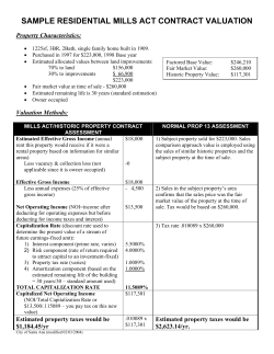

© Copyright 2026