
!! U. S. LENTIC WETLAND INVENTORY USER MANUAL (Current as of 6/6/2014)
!!
U. S. LENTIC WETLAND INVENTORY
USER MANUAL
(Current as of 6/6/2014)
This user manual is intended to accompany the U. S. Lentic Wetland Inventory Form for the inventory of still water (lentic)
wetlands. This document serves as a field reference to assist data collectors in answering each item on the form. It can also
serve as an aid to the database user in the interpretation of data presented in the U. S. Lentic Wetland Inventory format.
Another form entitled U. S. Lotic Wetland Inventory, with a different set of user guidelines, is available for lotic (flowing
water) wetlands.
!
!
ACKNOWLEDGEMENTS
!
!
BACKGROUND INFORMATION
Development of these assessment tools has been a collaborative and reiterative process. Many people from many agencies
and organizations have contributed greatly their time, effort, funding, and moral support for the creation of these documents,
as well as to the general idea of devising a way for people to look critically at wetlands and riparian areas in a systematic and
consistent way. Some individuals and the agencies/organizations they represent who have been instrumental in enabling this
work are Dan Hinckley, Tim Bozorth, and Jim Roscoe of the USDI Bureau of Land Management in Montana; Karen Rice
and Karl Gebhardt of the USDI Bureau of Land Management in Idaho; Bill Haglan of the USDI Fish and Wildlife Service in
Montana; Barry Adams and Gerry Ehlert of Alberta Sustainable Resource Development; Lorne Fitch of Alberta
Environmental Protection; Greg Hale and Norine Ambrose of the Alberta Cows and Fish Program, and Mike Frisina of the
Montana Department of Fish, Wildlife and Parks.
Flowing Water (Lotic) Wetlands vs. Still Water (Lentic) Wetlands
Cowardin and others (1979) point out that no single, correct definition for wetlands exists, primarily due to the nearly
unlimited variation in hydrology, soil, and vegetative types. Wetlands are lands transitional between aquatic (water) and
terrestrial (upland) ecosystems. Windell and others (1986) state, “wetlands are part of a continuous landscape that grades
from wet to dry. In many cases, it is not easy to determine precisely where they begin and where they end.”
!
In the semi-arid and arid portions of western North America, a useful distinction has been made between wetland types based
on association with different aquatic ecosystems. Several authors have used lotic and lentic to separate wetlands associated
with running water from those associated with still water. The following definitions represent a synthesis and refinement of
terminology from Shaw and Fredine (1956), Stewart and Kantrud (1972), Boldt and others (1978), Cowardin and others
(1979), American Fisheries Society (1980), Johnson and Carothers (1980), Cooperrider and others (1986), Windell and others
(1986), Environmental Laboratory (1987), Kovalchik (1987), Federal Interagency Committee for Wetland Delineation
(1989), Mitsch and Gosselink (1993), and Kent (1994).
!
Lentic wetlands are associated with still water systems. These wetlands occur in basins and lack a defined channel and
floodplain. Included are permanent (i.e., perennial) or intermittent bodies of water such as lakes, reservoirs, potholes,
marshes, ponds, and stockponds. Other examples include fens, bogs, wet meadows, and seeps not associated with a defined
channel.
!
Lotic wetlands are associated with rivers, streams, and drainage ways. They contain a defined channel and floodplain. The
channel is an open conduit, which periodically or continuously carries flowing water. Beaver ponds, seeps, springs, and wet
meadows on the floodplain of, or associated with, a river or stream are part of the lotic wetland.
!
Functional vs. Jurisdictional Wetland Criteria
Defining wetlands has become more difficult as greater economic stakes have increased the potential for conflict between
politics and science. A universally accepted wetland definition satisfactory to all users has not yet been developed because the
definition depends on the objectives and the field of interest. However, scientists generally agree that wetlands are
characterized by one or more of the following features: 1) wetland hydrology, the driving force creating all wetlands, 2)
hydric soils, an indicator of the absence of oxygen, and 3) hydrophytic vegetation, an indicator of wetland site conditions.
The problem is how to define and obtain consensus on thresholds for these three criteria and various combinations of them.
!
!
Manual current as of 6/6/2014
1!
Check www.ecologicalsolutionsgroup.com for latest dataset and manual
Wetlands are not easily identified and delineated for jurisdictional purposes. Functional definitions have generally been
difficult to apply to the regulation of wetland dredging or filling. Although the intent of regulation is to protect wetland
functions, the current delineation of jurisdictional wetland still relies upon structural features or attributes.
!
The prevailing view among many wetland scientists is that functional wetlands need to meet only one of the three criteria as
outlined by Cowardin and others (1979) (e.g., hydric soils, hydrophytic plants, and wetland hydrology). On the other hand,
jurisdictional wetlands need to meet all three criteria, except in limited situations. Even though functional wetlands may not
meet jurisdictional wetland requirements, they certainly perform wetland functions resulting from the greater amount of
water that accumulates on or near the soil surface relative to the adjacent uplands. Examples include some woody draws
occupied by the Fraxinus pennsylvanica/Prunus virginiana (green ash/chokecherry) habitat type and some floodplain sites
occupied by the Artemisia cana/Agropyron smithii (silver sagebrush/western wheatgrass) habitat type or the Pinus
ponderosa/Cornus stolonifera (ponderosa pine/red-osier dogwood) habitat type. Currently, many of these sites fail to meet
jurisdictional wetland criteria. Nevertheless, these sites do provide important wetland functions and may warrant special
managerial consideration. The current interpretation, at least in the western United States, is that not all functional wetlands
are jurisdictional wetlands, but all jurisdictional wetlands are functional wetlands.
!
Polygon Delineation
The lentic wetland inventory process incorporates data on a wide range of biological and physical categories. The basic unit
of delineation within which this data is collected is referred to as a polygon. A polygon is the area upon which one set of data
is collected. One inventory form is completed (i.e., one set of data is collected) for each polygon. One or more (usually
several) polygons constitute a project. A lentic (still water) wetland polygon is a wetland, or portion of a wetland, which is
not associated with a waterway (stream or river) and which has no defined channel. Polygons are delineated on topographic
maps before observers go to the field. It is important to clearly mark and number the polygons on the map.
!
If aerial photos are available, polygon delineations can be based on vegetation differences, geologic features, or other
observable characteristics. On larger systems with wide wetland areas, aerial photos may allow delineation of multiple
vegetation-based polygons away from the water source. In these cases, where polygons can be drawn as enclosed units a
minimum mapping unit of possibly 2 to 4 ha (5 to 10 ac) should be followed. The size of the minimum mapping unit should
be based on factors such as management capabilities, available funds, and capabilities of data collection.
!
If pre-delineated polygons are drawn on the maps, and pre-assigned numbers are given, be sure the inventoried polygons
correspond exactly to those drawn. Observers are allowed to move polygon boundaries, create new polygons, or consolidate
polygons if the vegetation, geography, location of fences, or width of the wetland zone warrant. If polygon boundaries are
changed, the changes must be clearly marked on the field copies of the maps. Observers should draw the complete polygon
boundary onto their field maps if possible at the 1:20,000 or 1:50,000 scale.
!
In most cases involving small bodies of water or small lentic wetlands, the inventoried polygon will be a single unit of area.
Around larger lakes, extensive marshes, or other large lentic wetlands, it may be necessary to divide the wetland into separate
polygons (Figure 1). Polygons should be divided at distinct locations such as fences, stream entrances or exits, or other
features easily recognized in the field. When selecting representative sites, consideration should be given to the differences
presented by landform position (i.e., point vs. bay, or windward vs. leeward side of the water body). Polygons should not
cross fences between areas with different management.
!
The outer boundaries of polygons are usually at the wetland ecosystem outer edges. These boundaries are sometimes easily
determined by abrupt changes in the landform and/or vegetation, but proper determination often depends on experienced
interpretation of more subtle features. Do not include deep water habitat within the polygon area. The inner polygon
boundary is the landward edge of the deep-water habitat, or where persistent emergent vegetation gives way to open water. In
concept, deep-water habitat is the area covered by surface water deeper than 2 m (6.6 ft), or where sunlight cannot penetrate
to support persistent, erect, rooted, plant life. Persistent emergent vegetation consists of species that normally remain standing
at least until the beginning of the next growing season, e.g., Typha species (cattails) or Schoenoplectus species (bulrushes). In
practice, include all emergent vegetation (i.e., go out to open water) regardless of depth. If emergent vegetation has been
removed by human activity, include out to where it would be expected in the absence of that impact. If there is no emergent
vegetation, and there is no apparent potential for it, then stop the polygon where persistent vegetation ends and the open
water begins.
!
!
In cases where observer access and visibility on part of the site to be assessed is impeded by deep water that may have
extensive areas of emergent vegetation, the observer may choose, with documented reason, to either:
Manual current as of 6/6/2014
2!
Check www.ecologicalsolutionsgroup.com for latest dataset and manual
•
•
•
!
Break the area into separate polygons in cases where large areas are utilized differently, such as where the landward
area (onshore) is heavily impacted by human use and the wetted area (marsh) is unimpacted;
Draw an arbitrary outer edge of the polygon that does not include all of the area with emergent vegetation, in which
case the observer must carefully document the delineation and the rationale employed; or
Include the entire dry and wet area together in a single polygon with careful commentary noting any areas that may
be impacted differently due to having such greatly different conditions.
When using the inventory on artificial or artificially enlarged water bodies (e.g. dugout, manmade pond, reservoirs), use the
same criteria, but remember that there will be questions that are difficult to apply appropriately. Focus on consistently
applying the methods, including site boundaries, as well as recording all decisions made in applying the methodology. The
goal of this exercise is to assess the ability of the site to perform riparian functions to its potential.
!
!
!
Figure 1. Schematic drawing of a lentic (still water) wetland showing: 1) delineation of polygons on larger
systems, i.e. those too big to inventory as a single polygon (more than about 1.6 km [0.5 mi] in length) or
those with managerial breaks crossing them; 2) a typical relationship between deep water habitat (lacking
emergent vegetation) and surrounding lentic wetland, which includes all areas of persistent emergent
vegetation in standing water.
!
!
!
INVENTORY FORM CODES AND INSTRUCTIONS
Class Codes
Field observers will use class codes to represent ranges of percent wherever percent data is recorded. The class codes are
defined below. These codes and range classes are from the USDA Forest Service Northern Regions ECODATA (1989)
program.
!
!
T = 0.1<1%
P = 1<5%
1 = 5<15%
2 = 15<25%
3 = 25<35%
4 = 35<45%
5 = 45<55%
6 = 55<65%
7 = 65<75%
8 = 75<85%
9 = 85<95%
F = 95-100%
The class codes are converted to class midpoints in the office. The class midpoints are: T = 0.5%; P = 3.0%; 1 = 10.0%; 2 =
20.0%; 3 = 30.0%; 4 = 40.0%; 5 = 50.0%; 6 = 60.0%; 7 = 70.0%; 8 = 80.0%; 9 = 90.0%; F = 97.5%. These class midpoints
are used in data reporting and in all calculations throughout the data analysis process.
!
!
Manual current as of 6/6/2014
3!
Check www.ecologicalsolutionsgroup.com for latest dataset and manual
Polygon Data
The following are the codes and instructions for the individual data items on the form. All data items are to be recorded in the
field unless otherwise noted. Numbering corresponds to that of items on the form. Also included are comments about the
data, how it is collected, and its meaning. When the inventory methodology follows a published source, that source is cited.
However, in many instances, due to the lack of pre-existing guidelines, we have developed our own methodologies.
!
Fill in all blanks on the field form, except those that are completed in the office. Enter 0 for any item to indicate the
absence of value. Do not use — and do not leave items blank, except for the following: 1) items that logically would not be
answered because they follow an answer of No in a leading Yes/No question, and 2) lines in a species list below the last
species observed. An answer of 0 means the observer looked and saw none, whereas a blank line means the observer did not
look, either by negligence or because the point was moot. NA means the item is not applicable to a particular polygon. NC
means data was not collected for that item in a particular polygon. Observers must write legibly and should limit their use of
abbreviations throughout to those, which allow for no confusion.
!
!
!
!
!
!
!
!
Record ID No. This is the unique identifier allocated to each polygon. This number will be assigned in the office when the
form is entered into the database.
Administrative Data
A1. Agency or organization collecting the data.
A2. Funding Agency/Organization.
A3a. BLM (Bureau of Land Management) State Office.
A3b. BLM Field Office/Field Station.
A3c. BLM Office Code (recorded in the office).
A3d. Is the polygon in an active BLM grazing allotment (recorded in the office)?
A3e, f. For BLM polygons, the BLM Office Code, whether the polygon is in an active BLM grazing allotment, and the
Allotment Number is supplied by the BLM. These items are entered into the computer in the office; the computer then
references a master list of Allotment ID’s to complete the remaining Allotment information. Because some polygons
incorporate more than one Allotment, space is provided to enter two sets of Allotment information. The master Allotment list
is periodically updated by the BLM National Applied Resource Sciences Center to make needed corrections.
!
!
!
!
!
!
!
!
!
!
A4. USDI Fish and Wildlife Service Refuge name.
A5. Indian Reservation name.
A6. USDI National Park Service Park/National Historical Site name.
A7. USFS (Forest Service) National Forest name.
A8. Other location.
A9. Year the field work was done.
A10. Date of field work by day, month, and year.
A11. Names of all field data observers.
NOTE: Information for items A12a-h is found in the office; field evaluators need not complete these items.
A12. The several parts of these items identify various ways in which a data record may represent a resampling of a polygon
that may have been inventoried again at some other time. The data in this record may have been collected on an area that
coincides precisely with an area inventoried at another time and recorded as another record in the database. It may also
!
Manual current as of 6/6/2014
4!
Check www.ecologicalsolutionsgroup.com for latest dataset and manual
represent the resampling of only a part of an area previously sampled. This would include the case where this polygon
overlaps, but does not precisely and entirely coincide with one inventoried at another time. One other case is where more than
one polygon inventoried one year coincides with a single polygon inventoried another year. All of these cases are represented
in the database, and all have some value for monitoring purposes, in that they give some information on how the status on a
site changes over time. This is done in the office with access to the database; field evaluators need not complete these
items.
!
!
A12a. Has any part of the area within this polygon been inventoried previously, or subsequently, as represented by any other
data record in the database? Such other records would logically carry different dates.
A12b. Does the areal extent of this polygon exactly coincide with that of any other inventory represented in the database? In
many cases, subsequent inventories only partially overlap spatially. The purpose of this question is to identify those records
that can be compared as representing exactly the same ground area.
!
!
!
!
!
!
!
!
!
!
!
!
A12c. Does this record represent the latest data recorded for this site (polygon)?
A12d. If A12b is answered Yes, then enter the record ID number(s) of any other previous or subsequent re-inventories
(resampling) of this exact polygon for purposes of cross-reference.
A12e. Enter the years of any records recorded in item A12d as representing other inventories of this exact polygon.
A12f. Even though this polygon is not a re-inventory of the exact same area as any other polygon, does it share at least some
common area with one or more polygons inventoried at another time?
A12g. Enter the years of any other inventories of polygons sharing common ground area with this one.
A12h. If A12f is answered Yes, then enter the record ID number(s) of any other polygon(s) sharing common ground area with
this one.
A13a. Has a management change been implemented on this polygon?
A13b. If A13a is answered Yes, in what year was the management change implemented?
A13c. If A13a is answered Yes, describe the management change implemented.
Location Data
B1. State in which the field work was done (recorded in the office).
B2. County or municipal district in which the field work was done (recorded in the office).
B3. This field for allotment,range, or management unit is intended for entities other than the BLM to use for grouping
polygons by management unit. The BLM management units are grouped using the grazing allotment information in A3
above.
!
!
!
B4a. For lentic polygons the area is usually listed as a lake name, or other local designation that identifies the area where the
inventory is conducted. If possible, use a name that is shown on the 7.5 minute topographic map.
B4b. Record the stream (if there is one) with which the inventoried lentic wetland is associated. Such association may be by
inlet or outlet surface flow, or by general ground water (sub surface) connection.
B4c, d. Polygons are grouped together for management purposes. For example, all polygons around Henry’s Lake in the
Idaho Falls Field Office could be identified as Group Name: Idaho Falls Field Office; Group Number: 1 (recorded in the
office).
!
!!
B5. Polygon number is a sequential identifier of the portion of the area assessed. This is referenced to the map delineations.
Sequences normally progress clockwise.
Manual current as of 6/6/2014
5!
Check www.ecologicalsolutionsgroup.com for latest dataset and manual
B6. Elevation (feet or meters) of the polygon midpoint. Elevation is interpolated from the topographic map(s).
!
!
!
B7a. Record the latitude and longitude of the polygon, along with the GPS projection and accuracy. Record the degrees,
minutes, and seconds, along with decimal degrees. NOTE: All of North America is latitude = North, and longitude = West.
B7b. Record any comments pertaining to the “other” location.
B8. Identity the hydrologic unit code(s) (HUC) associated with the reach of stream contained in the polygon are recorded.
The HUC data is obtained from the US Geological Survey (USGS) National Hydrography Dataset (NHD) (USGS 2012).
Based on the finest level of resolution available from the USGS for the stream reach, the levels of HUC information are
entered by the computer onto the form. The USGS has divided the nation into successively smaller hydrologic units, based on
drainage basins and watersheds. These units fit into hierarchical levels, uniquely identified by a pair of digits for each
successive level (i.e., an eight-digit number identifies a drainage at the fourth (subbasin) level; and a twelve digit HUC
identifies one at the sixth (subwatershed) level (Figure 2).
!
As defined by the USGS (2012), a hydrologic unit is “a drainage area delineated to nest in a multi-level, hierarchical
drainage system. Its boundaries are defined by hydrographic and topographic criteria that delineate an area of land upstream
from a specific point on a river, stream or similar surface waters. A hydrologic unit can accept surface water directly from
upstream drainage areas, and indirectly from associated surface areas such as remnant, non-contributing, and diversions to
form a drainage area with single or multiple outlet points. Hydrologic units are only synonymous with classic watersheds
when their boundaries include all the source area contributing surface water to a single defined outlet point.”
!
!
Provision is made on the data form for multiple HUC units, because a polygon may include all, or part, of more than one
HUC unit (especially when finer levels, such as the subwatershed [sixth] level, are identified).
The HUC data provided includes these items:
• HUC identification number to as many digits as have been delineated by USGS, down to the sixth level (12 digits);
• River miles of the stream from this HUC unit that fall within this polygon;
• Percent of the polygon stream reach that is located in this HUC unit (e.g., 100 percent if the entire polygon is all in
one HUC unit;
• Name of the region (first level of the HUC) (and its size in square miles);
• Name of the subregion (second level of the HUC) (and its size in square miles);
• Name of the basin (third level of the HUC) (and its size in square miles);
• Name of the subbasin (fourth level of the HUC) (and its size in square miles);
• Name of the watershed (fifth level of the HUC) (and its size in square miles); and
• Name of the subwatershed (sixth level of the HUC) (and its size in acres).
!
!
Manual current as of 6/6/2014
6!
Check www.ecologicalsolutionsgroup.com for latest dataset and manual
!
Figure 2. Hierarchy for the six nested levels of hydrologic units, as they are successively subdivided, and the numbering
scheme increases by two digits for each level of greater resolution (adapted from the USGS 2012)
!
Manual current as of 6/6/2014
7!
Check www.ecologicalsolutionsgroup.com for latest dataset and manual
!
Selected Summary Data
C1. Wetland/water body type is a categorical description of predominant polygon character. Select from the following list of
categories that may occur within a lentic system the one that best characterizes the majority of the polygon. Observers will
select only one category as representative of the entire polygon. If significant amounts of other categories are present,
indicate this in Vegetation Comments (item D17) or consider dividing the original polygon into two or more polygons.
!
——————————————————————————————————————————————————
Category Description
——————————————————————————————————————————————————
Wet Meadow. A grassland with waterlogged soil near the surface, but without standing water for most of the year. This type of wetland
may occur in either riparian (lotic) or in still water (lentic) systems. A lotic wet meadow has a defined channel or flowing surface
water nearby, but is typically much wider than the riparian zone associated with the classes described above. This is often the result of
the influence of lateral groundwater not associated with the stream flow. Lotic and lentic wet meadows may occur in proximity (e.g.,
when enough groundwater emerges to begin to flow from a mountain meadow, the system goes from lentic to lotic). Such
communities are typically dominated by herbaceous hydrophytic vegetation that requires saturated soils near the surface, but tolerates
no standing water for most of the year. This type of wetland typically occurs as the filled-in basin of old beaver ponds, lakes, and
potholes.
Marsh. A frequently or continually inundated wetland characterized by emergent herbaceous vegetation adapted to saturated soil
conditions. A marsh generally has a mineral soil substrate does not accumulate peat.
Fen. A peat-accumulating wetland that receives some drainage from surrounding mineral soil and usually supports marsh-like vegetation.
Bog. A peat-accumulating wetland that has no significant inflows or outflows and supports acidophilic mosses, particularly sphagnum.
Spring/Seep. Groundwater discharge areas. In general, springs have more flow than seeps. This wetland type may occur in a riparian
(lotic) or still water (lentic) system.
Reservoir. An artificial (dammed) water body with at least 8 ha (20 ac) covered by surface water.
Stock pond. An artificial (dammed) body of water of less than 8 ha (20 ac) covered by surface water.
Lake. A natural topographic depression collecting a body of water covering at least 8 ha (20 ac) with surface water.
Pothole, Slough, or Small Mountain Lake. A natural topographic depression collecting a body of water covering less than 8 ha (20 ac)
with surface water.
Other. Describe any other wetland type encountered, which is not associated with a surface water channel.
Upland. This designation is for those areas which are included in the inventoried polygon, but which do not support functional wetland
vegetation communities. Such areas may be undisturbed inclusions of naturally occurring high ground or such disturbed high
ground as roadways and other elevated sites of human activity.
——————————————————————————————————————————————————
!!
C2. The size (acres/hectares) of polygons large enough to be drawn as enclosed units on topographic maps is determined in
the office using a planimeter, dot grid, or GIS. For polygons too small to be accurately drawn as enclosed units on the maps,
polygon size is calculated using polygon length (item C5) and average polygon width (item C7a).
!
C3a-d. Evaluators may be asked to survey some areas that have not been determined to be wetlands for the purpose of
making such a determination. Other polygons include areas supporting non-wetland vegetation types. A Yes answer indicates
that no part of the polygon keys to a riparian habitat type or community type (HT/CT). Areas classified in item D15 as any
vegetation type described in a riparian and/or wetland classification document for the region in which you are working are
counted as functional wetlands. Areas listed as UNCLASSIFIED WETLAND TYPE are also counted as functional wetlands.
Other areas are counted as non-wetlands, or uplands. The functional wetland fraction of the polygon area is listed in item C3c
in acres and as a percentage of the entire polygon area in item C3d.
!
C4. Lentic wetlands associated with open water, like lakes and ponds, typically have a shore. The shore is defined as a
variable width area that contains all points reached over time by the water’s edge along the water body between its high stage
and current water level—i.e., the area that is visibly affected by periods of inundation and drying between seasonal and
longer cyclic high and low water levels. (The time frame is generally taken to mean the recent period of hydrologic record, or
the extent indicated by physical evidence present.) The shoreline is defined much more narrowly as a 1-2 m (3.3-6.6 ft) band
stretching along the landward side of the water’s edge TODAY. A defined shoreline means there is narrow band or line that is
distinctive and distinguishable. Therefore, the actual position of the shoreline shifts over time with water level.
!
!
Manual current as of 6/6/2014
8!
Check www.ecologicalsolutionsgroup.com for latest dataset and manual
Some lentic polygons may not contain a shore between wetland and open water. In some cases these polygons are in
ephemeral depressions which may be infrequently inundated, but do support wetland plant communities. In other cases, these
polygons may be part of large marsh systems that may or may not be associated with lakes, but where polygons may be
delineated in areas not adjacent to open water.
!
C5. Polygon length is measured in the field or by scaling from the map. This data is considered accurate to the nearest 0.16
km (0.1 mi). Polygon length may be the same as shoreline length, but may not be in cases of much curved shoreline, or for
polygons that have no shoreline (i.e., wet meadows or marshes). The shoreline is defined as a linear feature extending at the
time of observation along the water’s edge 1 m (3 ft) wide back from the water onto the land.
!
C6. In some cases, the polygon data is used to characterize, or represent, a much larger, or longer, area. The length
represented by the polygon is given. For example, a 0.8 km (0.5 mi) polygon may be used to represent 3.2 km (2 mi) of total
shoreline length. In this case, 0.8 km (0.5 mi) is the shoreline length in the polygon (item C5), and 3.2 km (2 mi) is the
overall shoreline length entered in item C6.
!
C7a. Record average width of the polygon, which in smaller wetlands corresponds to the width of the entire wetland area.
The width (average, minimum and maximum) will be determined in the field as the distance perpendicular to the longest
axis.
!
!
C7b. Record the range of width (ft/m), narrowest to widest, of the wetland area in the polygon.
Health Assessment Summary
C8. Polygon Health (PFC) Score is an ecological function rating derived by computer using data from several items in the
polygon inventory. For detailed discussion of this process, see the companion document Lentic Wetland Health Assessment
(derived from the Lentic Wetland Inventory Form). The techniques used to obtain the data do not allow the ratings to be
interpreted with a fine degree of precision. For example, two polygons rating 74% and 79% should be interpreted as
functionally equivalent to each other, but they both are likely to differ functionally from a third polygon that rates 61%,
although all three fall within the Functional At Risk (Healthy, but with Problems) category. When considering the health
assessment result for any site, one should always look at the individual items, as well as the total score. Two sites can score
overall identical results, but have profoundly differing areas of problems.
!
!
The health ratings are presented both as an overall polygon score and in two subsections (vegetation and physical site) to give
a broad indication of what part of the system may be in need of more management attention.
Vegetation Data
D1a. The United States of America and its territories are geographically divided into 10 distinct wetland delineation regions
by the U.S. Army Corps of Engineers (Lichvar 2012) as shown in Figure 3. The National Wetland Plant List has assigned a
wetland indicator status for each plant species on the list according to those wetland regions they occur in. Selecting the
proper wetland delineation region is essential because this is used to calculate the wetland prevalence index.
!
!
Manual current as of 6/6/2014
9!
Check www.ecologicalsolutionsgroup.com for latest dataset and manual
!
Figure 3. U.S. Army Corps of Engineers wetland delineation regions of the United States of America (Lichvar 2012)
!!
Three U.S. Army Corps of Engineers wetland delineation regions cover the contiguous western United States of America: the
Great Plains Region (Figure 4), the Western Mountains, Valleys, and Coast Region (Figure 5), and the Arid West Region
(Figure 6). Subregions identified on the maps correspond to USDA Land Resource Regions, however the observer need only
identify the primary wetland delineation region the polygon is in. It should be noted that isolated mountainous areas such as
the Black Hills, Arizona Mountains, and New Mexico Mountains are included within the Western Mountains, Valleys, and
Coast Region.
!
!
Manual current as of 6/6/2014
!
10
Check www.ecologicalsolutionsgroup.com for latest dataset and manual
!
Figure 4. The Great Plains Region and Subregions.
!!
!
Manual current as of 6/6/2014
!
11
Check www.ecologicalsolutionsgroup.com for latest dataset and manual
!
Figure 5. The Western Mountains, Valleys, and Coast Region and Subregions.
!!
!
Manual current as of 6/6/2014
!
12
Check www.ecologicalsolutionsgroup.com for latest dataset and manual
!
Figure 6. The Arid West Region and Subregions.
!!
D1b. The wetland prevalence index is compiled by the computer from the U.S. National Wetland Inventory (NWI) wetland
status classes for plant species recorded on the site (Lichvar 2012) and weighted by species abundance measured in terms of
canopy cover. The range of index values is from 1.0 to 5.0. Lower values indicate wetter sites.
!
D1c. The vegetation structural diversity category is automatically calculated in the office by computer using plant group and
height layer data (item D9). Trees and shrubs are considered major components of structural diversity. These terms are used
to describe vegetation height: tall = > 1.8 m (6.0 ft) (layer 3); medium = >0.5-1.8 m (1.5-6.0 ft) (layer 2); short = 0-0.5 m
(0-1.5 f) (layer 1). Graminoids and forbs are combined as the herbaceous lifeform. Trees and shrubs in layer 2 are also
!
Manual current as of 6/6/2014
!
13
Check www.ecologicalsolutionsgroup.com for latest dataset and manual
combined as medium trees/ shrubs. A polygon is assigned the highest structural diversity category it can meet. To meet a
category, each lifeform (by height) named in the description must have a canopy cover of at least 15% in the polygon.
Combination groups (i.e., medium trees/shrubs; and short, medium, and tall herbaceous) must have at least 5% cover of both
components or at least 15% cover of one component. NOTE: Structural diversity on a site can change as succession proceeds
or if management changes.
!
——————————————————————————————————————————————————
Category Description
——————————————————————————————————————————————————
Tall trees; tall shrubs; medium trees/shrubs; herbaceous understory present1
Tall trees; tall shrubs; herbaceous understory present1
Tall trees; medium trees/shrubs; herbaceous understory present1
Tall trees; herbaceous understory present1
Tall shrubs; medium trees/shrubs; herbaceous understory present1
Tall shrubs; herbaceous understory present1
Medium trees/shrubs; herbaceous understory present1
Tall herbaceous
Medium herbaceous
Short herbaceous
Sparsely vegetated2
——————————————————————————————————————————————————
1The
herbaceous understory present does not need to have a minimum canopy cover.
vegetated refers to polygons in which the minimum canopy cover by the various lifeforms is not met.
2Sparsely
!!
D2a, b. If present, record the 6-letter species code and the canopy cover in the two left-most columns for ALL tree species
observed. Canopy cover is evaluated using ocular estimation following the Daubenmire (1959) method. Within the total
canopy cover of each species, estimate the proportion of each of five groups (seedling, sapling, pole, mature, and dead trees).
The canopy covers of the five groups of each species must total approximately 100%. If some individuals in an age group
have at least 30% of the upper canopy dead (are decadent), record the decadence as a percentage of that group. Record the
total group cover to the left of the slash (/) and the decadent portion to the right.
!
!
Example:
Species
Cover
Sdlg/Dec
Splg/Dec
Pole/Dec
Mat/Dec
Dead
POPBAL
3
T/0
P/0
1/P
8/1
P
Note 1: The most common usage of the term decadent may be for over mature trees past their prime and which may be
dying, but we use the term in a broader sense. We count decadent plants, both trees and shrubs, as those with 30% or more
dead wood in the upper canopy. In this item, scores are based on the percentage of total woody canopy cover which is
decadent or dead, not on how much of the total polygon canopy cover consists of dead and decadent woody material. Only
decadent and dead standing material is included, not that which is lying on the ground. The observer is to ignore (not count)
decadence in poplars or cottonwoods which are decadent due to old age (rough and furrowed bark extends substantially up
into the crowns of the trees) (species: Populus deltoides [Great Plains cottonwood], P. angustifolia [narrowleaf cottonwood],
and P. balsamifera [black cottonwood]), because cottonwoods/poplars are early seral species and naturally die off in the
absence of disturbance to yield the site to later seral species. The observer is to consider (count) decadence in these species if
apparently caused by de-watering, browse stress, climatic influences, or parasitic infestation (insects/disease). The observer
should comment on conflicting or confounding indicators, and/or if the cause of decadence is simply unknown (but not due to
old age).
!
!!
!!
!!
!!
Note 2: Do not count the resprouts from cut-off stumps as regeneration of a plant that was cut. As a general rule, count
sprouts ONLY that emanate from the soil, and NOT from the stem above ground.
Manual current as of 6/6/2014
!
14
Check www.ecologicalsolutionsgroup.com for latest dataset and manual
Tree Age Groups
——————————————————————————————————————————————————
Conifers1 and Cottonwoods/Poplars
Age Group
Other Broadleaf Species 2
——————————————————————————————————————————————————
Seedling
Sapling
Pole
Mature
Dead
<4.5 ft tall OR <1.0 inch dbh
≥4.5 ft tall AND 1.0 inch to 4.9 inch dbh
5.0 inch to 8.9-inch dbh
> 9.0-inch dbh
100% of canopy is dead
<3.0 ft tall
>3.0 ft tall AND <3.0 inch dbh
>6.0 ft tall AND 3.0 inch to 5.0-inch dbh
>5.0-inch dbh
100% of canopy is dead
——————————————————————————————————————————————————
1Juniperus
scopulorum (Rocky Mountain juniper) is an exception to the specifications given, because it lacks typical coniferous size, age,
and growth form relationships. Assign age classes to individuals based on relative size, reproductive ability, and overall appearance.
2Other Broadleaf Species may include Fraxinus pennsylvanica (green ash), Acer negundo (box elder), Populus tremuloides (quaking
aspen), Betula papyrifera (paper birch), and Ulmus americana (American elm).
!!
Note 3: For field determination of vegetative cover related questions (questions D2 to D14) include all rooted plant material
(live or dead). Do not include fallen wood or other plant litter. Do not consider the polygon area covered by water (such as
between emergent plants).
!
D3. The tree regeneration category is automatically calculated in the office by the computer using the age group data
collected with the species’ canopy cover as described in item D2b. The canopy covers of the seedling and sapling age groups
are combined to quantify tree regeneration. The categories represent actual, not potential, tree regeneration.
!
——————————————————————————————————————————————————
Code
Description
——————————————————————————————————————————————————
1
No seedlings or saplings were observed in the polygon.
2
3
4
5
Seedlings and/or saplings were observed; individually, or in combination, these age groups have less than 5% of the
species canopy cover.
Seedlings and/or saplings were observed; individually, or in combination, these age groups have 5% or more of the
species canopy cover, but less than 15%.
Seedlings and/or saplings were observed; individually, or in combination, these age groups have 15% or more of the
species canopy cover, but less than 25%.
Seedlings and/or saplings were observed; individually, or in combination, these age groups have 25% or more of the
species canopy cover.
——————————————————————————————————————————————————
!!
D4. The tree age group distribution category is automatically calculated in the office by the computer using age group canopy
covers recorded in item D2b. In classifying tree age group distribution, the seedling and sapling groups are combined. Three
resulting age groups (seedlings/saplings, pole, and mature), and the percent of the mature individuals which are decadent,
determine age group distribution categories.
!
Decadence of younger age groups is ignored in this calculation. Younger decadent trees are assumed to have the capacity to
grow out of any current condition caused by injury, disease, or other non-age related factors. A species with decadent mature
individuals may fall into one of two classes: those having 75% or more of mature individuals decadent and those having less
than 75% of mature individuals decadent. The age distribution category of a tree species on a polygon is defined by the
presence of certain age groups. To be present, age groups must have minimum canopy covers in the polygon: seedlings/
saplings must have a combined total canopy cover of at least 1%; pole and mature are treated separately and must each have
at least 5% canopy cover.
!!
!!
!!
!
Manual current as of 6/6/2014
!
15
Check www.ecologicalsolutionsgroup.com for latest dataset and manual
Tree Age Group Distribution Categories (An X under an age group indicates presence in that category.)
——————————————————————————————————————————————————
Category
Code
Sdlg1/Splg2
(CC >1%)
Pole
(CC >5%)
Mature (Decadent3)
(CC>5%)
Description
——————————————————————————————————————————————————
1
X
seedling/sapling only
2
X
pole age only
3
X
X
seedling/sapling and pole
4
X
X
seedling/sapling and mature (<75% dec.)
5
X
X
pole and mature (<75% dec.)
6
X
X
X
seedling/sapling, pole, and mature (<75% dec.)
7
X
mature only (<75% dec.)
8
X
X
seedling/sapling and mature (≥75% dec.)
9
X
X
pole and mature (≥75% dec.)
10
X
X
X
seedling/sapling, pole, and mature (≥75% dec.)
11
X
mature only (≥75% dec.)
——————————————————————————————————————————————————
1Sdlg
!
!
indicates seedlings, Splg indicates saplings, Decadent indicates percent of mature trees, which are decadent
D5a. Record the appropriate category, that best describes the amount of browse utilization (Utl) of the combined seedling
(Sdlg) and sapling (Splg) age groups for each tree species. When estimating amount of utilization, count browsed second year
and older leaders on representative plants of tree species normally browsed by ungulates. Do not count current year’s use,
because this would not accurately reflect actual use when more browsing can occur later in the season. Browsing of second
year or older material affects the overall health of the plant and continual high use will affect the plant’s ability to maintain
itself on the site. Determine percentage by comparing the number of leaders browsed or utilized with the total number of
leaders available (those within animal reach) on a representative sample (at least three plants) of each tree species present. Do
not count utilization on dead plants, unless it is clear that death resulted from over-grazing. NOTE: If a shrub is entirely
mushroom/umbrella shaped by long term intense browse or rubbing, count utilization of it as heavy.
!
——————————————————————————————————————————————————
Category
Description
——————————————————————————————————————————————————
None
Light
Moderate
Heavy
Unavailable
NA
0 to 5% of the available second year and older leaders are clipped (browsed).
>5 to 25% of the available second year and older leaders are clipped (browsed).
>25 to 50% of the available second year and older leaders are clipped (browsed).
More than 50% of the available second year and older leaders are clipped (browsed).
Woody plants provide no browsed or unbrowsed material below 1.5 m (5 ft), or are inaccessible due to
location or protection by other plants.
Neither seedlings nor saplings of tree species are present.
——————————————————————————————————————————————————
!!
D5b. Referring to Keigley and Frisina (1998), characterize seedling and sapling plants (if any) of each tree species by growth
architecture type. Polygons will likely exhibit a range of effects caused by browse, therefore choose a best fit category to
represent the majority condition for plants of each species. Categories are:
Uninterrupted—The plant has gain height each growing season; has at least one stem that not has no entire annual segment
killed by browsing.
Arrested—A plant that has had intense browsing all its life; it is hedged from above.
Retrogressed—The plant grew normally in early life, but was switched to intense browse later in life.
Released—A plant that had intense browsing early in life, but later was switched to lighter use, and allowed to grow taller.
!
!
!
D5c. Referring to Keigley and Frisina (1998) and more recent illustrations (Figure 4a-d) (Keigley and Frisina [in press])
choose one of two categories of browse intensity: Light-to-Moderate or Intense.
Manual current as of 6/6/2014
!
16
Check www.ecologicalsolutionsgroup.com for latest dataset and manual
!
!
Figure 4a, b. Illustrations of sequences of Light-to-Moderate browsing and Intense browsing (from Richard Keigley 2008)
!
!
!
Figure 4c, d. Another sequence of Intense browsing how to recognize Intense browsing (from Richard Keigley 2008)
!
Manual current as of 6/6/2014
!
17
Check www.ecologicalsolutionsgroup.com for latest dataset and manual
!
D5d. Estimate the overall proportion (percentage) of all cottonwood regeneration on the polygon (seedlings and saplings of
Populus species other than P. tremuloides [quaking aspen]) that are from seed, rather than from any form of asexual
reproduction, such as root sprouts.
!
D6a, b. Are there shrubs present on the polygon, and does the polygon have potential for woody species, such as tall shrubs
and trees? Some riparian and wetland sites are marshes, wet meadows, or other wetland types that lack potential for woody
species. Such sites should not be penalized on health assessment rating for this lack of potential. Other sites lacking these
species do have the potential, but lack the plants due to disturbance. Observers are to answer D6b on the basis of species
noted on similar, nearby, less disturbed sites, or other indications. On polygons where the observer cannot find sufficient
evidence to make a confident determination, enter NC and explain in the comment field at the end of the Vegetation Section.
!
D6c. Record the species code and canopy cover for every shrub species observed on the polygon. Determine the portion of
the species cover represented by each of three groups: seedling/saplings, mature, or decadent/dead. (NOTE: For shrubs, all
decadent individuals are included in one group with dead individuals. This contrasts to the method of recording tree
decadence, where the decadence within each age group is recorded.) As with trees, decadent shrubs are individuals having
30% or more dead material in the canopy. The canopy covers of the three age/size groups for a species must total
approximately 100%.
!
In general, shrub seedling/saplings can be distinguished from mature plants on the following basis: For normally tall shrubs,
which have an average mature height of over 1.8 m (6.0 ft), seedlings and saplings will be plants reaching only into the first
and second vegetation layers (shorter than 1.8 m [6.0 ft]). For shrub species having normal mature height between 0.5 m (1.5
ft) and 1.8 m (6.0 ft), seedlings and saplings are individuals reaching only into the first vegetation layer (below 0.5 m [1.5
ft]). For short shrub species, whose mature height is 0.5 m (1.5 ft) or less, observers must judge individual plants for height,
reproductive structures, and other characteristics that indicate relative age. Refer to reference manuals on the regional flora
for information of normal sizes for unfamiliar species. Remember that browsing may have shortened the stature of mature
specimens.
!
When estimating degree of utilization, count browsed second year and older leaders on representative plants of woody
species normally browsed by ungulates. Do not count current year’s use, because this would not accurately reflect actual use
when more browsing can occur later in the season. Browsing of second year or older material affects the overall health of the
plant and continual high use will affect the plant’s ability to maintain itself on the site. Determine percentage by comparing
the number of leaders browsed or utilized with the total number of leaders available (those within animal reach) on a
representative sample (at least three plants) of each shrub species present. Do not count utilization on dead plants, unless it is
clear that death resulted from over-grazing. NOTE: If a shrub is entirely mushroom/umbrella shaped by long term intense
browse or rubbing, count utilization of it as heavy. Record to the right of the slash (/) the one category that best describes
shrub utilization for each age group (using the five categories in item D5 above).
Example:
!
!
Species
ALNINC
Cover
2
Sdlg-Splg/Util
P / Moderate
Mature/Util
7 / Light
Dec-Dead/Util
3 / Unavail.
Shrub Growth Form
N
D6d. Record the category best describing the dominant appearance of each shrub species in the polygon.
——————————————————————————————————————————————————
Code
Description
——————————————————————————————————————————————————
N
Normal Growth Form. No apparent deviation from the normal appearance of the lifeform.
F
Flat-Topped Growth Form. Shrubs with the tallest leaders hedged (e.g., hedging from the top down). (Moose
U
C
during winter in deep snow browse exposed branches of shorter plants.)
Umbrella-shaped/Heavily-hedged/High-lined. Shrubs that have most of the branches (up to 1.5 m [1.5 ft] in
height) removed by browsing.
Cut Off at or Near the Ground. Shrubs that have been cut off by beaver or humans, at or near the base of the main
stem(s).
——————————————————————————————————————————————————
!!
!
Manual current as of 6/6/2014
!
18
Check www.ecologicalsolutionsgroup.com for latest dataset and manual
D6e. For each shrub species listed, record the type of architecture caused by browsing. Follow Keigley and Frisina (1998) in
determining the architecture type. Refer to the Keigley and Frisina (1998) document (Browse Evaluation by Analysis of
Growth Form) for greater detail and illustrations for this determination. Evaluate typical specimens of each species observed
in making the determination. On some polygons there may be multiple situations causing different architecture types in the
same species to occur (i.e., when there are areas of different accessibility within the polygon, causing browsing intensity to be
greater in places). In such cases, enter multiple types for the species in descending order of the relative abundance (i.e., enter
the type representing the greatest number of plants first, etc.). On the field data form, enter the codes from the table below.
——————————————————————————————————————————————————
Architecture Type
Description
——————————————————————————————————————————————————
Uninterrupted
Arrested
Retrogressed
Released
The terminal leader of the plant has not had an annual growth segment killed by browsing.
The plant has been intensely browsed all its life, and no stem has escaped having an entire annual segment killed.
After a period of light-to-moderate browsing early in life, the plant then is intensely browsed from above
An arrested or retrogressed plant has had the intense browsing removed and has been allowed to resume normal
vertical growth
——————————————————————————————————————————————————
!
D6f. For each shrub species listed, record the level of browse intensity that characterizes usage of that species throughout the
polygon. This is a generalization that acknowledges there is typically a range of usage levels determined by differing degrees
of accessibility and animal movement patterns across the polygon. Follow Keigley and Frisina (1998) to determine which of
the two levels of browse intensity (Intense or Light-to-Moderate) represents the predominant condition on the polygon.
Browsing is Intense when a complete annual segment is killed. Describe wide variations in level of use that might exist and
the reasons for it in the comment field (D17).
!
D6g. (Skip this item if the polygon lacks trees and shrubs AND there are no stumps or cut woody plants to indicate that it
ever had any.) Excessive cutting or removing parts of plants or whole plants by agents other than browsing animals (e.g.,
human clearing, cutting, beaver activity, etc.) can result in many of the same negative effects to the community that are
caused by excessive browsing. However, other effects from this kind of removal are direct and immediate, including
reduction of physical community structure and wildlife habitat values. Do not include natural phenomena such as natural
fire, insect infestation, etc. in this evaluation.
!
Removal of woody vegetation may occur at once (timber harvest), or it may be cumulative over time (annual firewood
cutting or beaver activity). This question is not so much to assess long term incremental harvest, as it is to assess the extent
that the stand is lacking vegetation that would otherwise be there today. Give credit for re-growth. Consider how much the
removal of a tree many years ago may have now been mitigated with young replacements.
!
Three non-native species or genera are excluded from consideration because these are aggressive, invasive exotic plants that
should be removed. They are Elaeagnus angustifolia (Russian olive), Rhamnus cathartica (common buckthorn), and Tamarix
species (saltcedar; tamarisk).
!
Determine the extent to which woody vegetation (trees and shrubs) is lacking due to being physically removed (i.e., cut,
mowed, trimmed, logged, cut by beaver, or otherwise removed from their growing position). The timeframe is less important
than the ecological effect. Time to recover from this kind of damage can vary widely with site characteristics. The objective is
to measure the extent of any damage remaining today to the vegetation structure resulting from woody removal. We expect
that the woody community will recover over time (re-grow), just as an eroding bank will heal with re-growing plant roots.
This question simply asks how much woody material is still missing from what should be on the site? The amount of time
since removal doesn't really matter, if re-growth has been allowed to progress. If 20 years after logging, the site has a stand of
sapling spruce trees, then it should get partial re-growth credit, but not full credit, since the trees still lack much of their
potential habitat and ecological value. (NOTE: In general, the more recent the removal, the more entirely it should be fully
counted; and conversely, the older the removal, the more likely it will have been mitigated by re-growth.)
!
This question is really looking at volume (three dimensions) and not canopy cover (two dimensions). For example, if an old
growth spruce tree is removed, a number of new seedlings/saplings may become established and could soon achieve the same
canopy cover as the old tree had. However, the value of the old tree to wildlife and overall habitat values is far greater than
that of the seedling/saplings. It will take a very long time before the seedlings/saplings can grow to replace all the lost habitat
values that were provided by the tall old tree. On the other hand, shrubs, such as willows, grow faster and may replace the
volume of removed plants in a much shorter time. Answer this question by estimating the percent of woody material that is
!
Manual current as of 6/6/2014
!
19
Check www.ecologicalsolutionsgroup.com for latest dataset and manual
missing from the site due to having been removed by human action. Select a range category from the choices given that best
represents the percent of missing woody material.
!
!
D6h. Record comments giving evidence for the above call.
D7 and D8. Record the species code and the percent canopy cover for graminoid and forb species observed in the polygon.
As a minimum, include all species having at least 5% cover on the polygon. This inventory is not intended to be
comprehensive. It is not necessary to search for obscure species, just record all species readily seen. Observers should
especially look, however, for hydrophytic (wetland) species that may be reduced to trace representation by site disturbance.
Herbaceous species other than invasive plant species (see item D13) with minor presence may be overlooked without serious
compromise to the inventory value.
!
D9. The purpose of this item is to describe the vegetation structure in terms of height layers and plant lifeforms on the
polygon. (Think of the layering as though it were a GIS file with 12 layers, each one representing one of four lifeforms [trees,
shrubs, graminoids, and forbs] in one of three height layers.) Include the canopy cover on the polygon that is provided by all
rooted plants (live or dead). Do not include fallen wood or other plant litter. Do not consider the polygon area that is covered
by water (such as between emergent plants).
!
Record the percent canopy cover of each plant lifeform in each of the three height layers. Consider each group in each layer
separately. For example, shrubs in layer 2 will be the canopy cover of all plants of all shrubs in the polygon between >0.5 m
(1.5 ft) and 1.8 m (6.0 ft) tall (roughly knee high to head high). In estimating this value, ignore all plants taller and shorter
than this range. Similarly, estimate the cover separately of those taller and those shorter shrubs. Proceed in this way through
each lifeform and layer. As a check, refer to your species/canopy lists to help remember what all you have seen on the site.
Leave no field blank; enter 0 to indicate absence of a value. (A blank field means the observer forgot to collect the data; a
value means the observer looked.) See further discussion in the note for item D10.
!
D10. Record the total percent of the polygon area occupied by canopy cover of each plant lifeform. Include the canopy cover
on the polygon that is provided by all rooted plants (live or dead). Do not include fallen wood or other plant litter. Do not
consider the polygon area that is covered by water (such as between emergent plants). Avoid counting overlapping areas more
than once for one group. (For example, an area is not counted twice for total tree cover if seedlings cover all ground under
mature trees.) However, the same piece of ground may occur under the canopy of more than one group. (For example, areas
covered by grass which are also under trees would be counted for both tree and grass lifeforms.) On the other hand, when
estimating total cover of all plants (item D12), the area covered by both trees and grass would only be counted once—trees
and grass in this case being part of the same group (all four plant groups).
!
D11. Record the percent of the polygon area covered by tree and shrub (woody species) canopy considered as a group in the
sense described above. Include the canopy cover on the polygon that is provided by all rooted plants (live or dead). Do not
include fallen wood or other plant litter. Do not consider the polygon area that is covered by water (such as between emergent
plants).
!
D12. Record the percent of the polygon area covered by the canopy of all four plant groups together. Include the canopy
cover on the polygon that is provided by all rooted plants (live or dead). Do not include fallen wood or other plant litter. Do
not consider the polygon area that is covered by water (such as between emergent plants).
!
D13a, b. Invasive plants (noxious weeds) are alien species whose introduction does or is likely to cause economic or
environmental harm. Without regard to whether the disturbance that allowed their establishment is natural or human-caused,
weed presence indicates a degrading ecosystem. While some of these species may contribute to some riparian functions, their
negative impacts reduce overall site health. This item assesses the degree and extent to which the site is impacted by the
presence of noxious weeds. The severity of the weed problem on a site is a function of density/distribution (pattern of
occurrence), as well as abundance of the weeds. A weed list should be used that is standard for the region.
!
Record the combined percent canopy cover and the overall density distribution class of all invasive plants on the polygon.
Common invasive plant species are listed on the form. Leave no listed species field blank, however; enter 0 to indicate
absence of a species. (A blank field means the observer forgot to collect the data; a value means the observer looked.) For
each weed species observed record canopy cover as a percentage of the polygon (area being evaluated) and density/
distribution class. Choose a density/distribution class from the chart (Figure 5) below that best represents each species’
pattern of presence on the site.
!
Manual current as of 6/6/2014
!
20
Check www.ecologicalsolutionsgroup.com for latest dataset and manual
!
!
!
Figure 5. Invasive plant species class guidelines (figure adapted from Adams and others [2003])
D13c. Record total presence of all invasive plant species on the polygon. Use the same method described above without
consideration of individual species, but instead by considering all weed species together as though they were one. Enter the
total canopy cover of all invasive plant species and the density/distribution class of all invasive plant species considered
together.
!
D14a, b. Areas with historically intense grazing often have large canopy cover of undesirable herbaceous species, which tend
to be less productive and which contribute less to ecological functions. A large cover of disturbance-increaser undesirable
herbaceous species, native or exotic, indicates displacement from the potential natural community (PNC) and a reduction in
upland health. These species generally are less productive, have shallow roots, and poorly perform most upland functions.
They usually result from some disturbance, which removes more desirable species. Invasive plant species considered in the
previous item are not reconsidered.
!
A list of disturbance-increaser undesirable species that are counted is presented below. Other disturbance-increaser
undesirable species may also be present on a site, but consistency and comparability will be maintained by always counting
the same set of species.
!
Achillea millefolium (common yarrow)
Artemisia ludoviciana (cudweed sagewort)
Juncus balticus (Baltic rush)
Mentha arvense (field mint)
Potentilla anserina (silverweed)
Thlaspi arvense (field pennycress)
!
Agropyron repens (quackgrass)
Descurainia sophia (fixweed)
Lepidium perfoliatum (clasping pepperweed)
Plantago major (common plantain)
Sisymbrium species (tumblemustard)
Trifolium species (clover)
Antennaria species (everlasting; pussytoes)
Fragaria virginiana (wild strawberry)
Medicago lupulina (black medick)
Poa pratensis (Kentucky bluegrass)
Taraxacum officinale (common dandelion)
Verbascum thapsus (common mullein)
D15. List the riparian habitat type(s) and/or community type(s) found in the polygon using a manual for identifying types in
the region in which you are working, such as Classification and Management of Montana’s Riparian and Wetland Sites
(Hansen and others 1995), Classification and Management of USDI Bureau of Land Management’s Riparian and Wetland
Sites in Eastern and Southern Idaho (Hansen and Hall 2002), Classification and management of upland, riparian, and
wetland sites of USDI Bureau of Land Management’s Miles City Field Office, eastern Montana USA (Hansen and others
2008), or a similar publication written for the region in which you are working. If the habitat type cannot be determined for a
!
Manual current as of 6/6/2014
!
21
Check www.ecologicalsolutionsgroup.com for latest dataset and manual
portion of the polygon, then list the appropriate community type(s) of that portion. If neither the habitat type nor community
type can be determined for any portion of the polygon (or in areas where the habitat and community types have not been
named and described), list the area in question as unclassified wetland type and give the dominant species present. Indicate
with the appropriate abbreviation if these are habitat types (HT), community types (CT), or dominance types (DT), for
example, PSEMEN/CORSTO HT. For each type listed, estimate the percent of the polygon represented. If known, record the
successional stage (i.e., early seral, mid-seral, late seral, and climax), or give other comments about the type. As a minimum,
list all types which cover 5% or more of the polygon. The total must approximate 100%. Slight deviations due to use of class
codes or to omission of types covering less than 5% of the polygon are allowed. NOTE: For any area classified as an
unclassified wetland type, it is important to list any species present which can indicate the wetness or dryness of the site.
!
!
NOTE: Open water in the polygon that does not have emergent vegetation, but that is less than 2 m (6.6 ft) deep is counted as
a type called Open Water.
D16a-c. Fire plays an important role on shaping our landscape. Fire can dramatically alter the vegetational expression of a
polygon, especially woody vegetation. This question pertains to the more recent fire history and its affect on the polygon.
Respond “Yes” to D16a only if the polygon vegetation is deemed currently to be altered from what it would otherwise be, by
having burned. For example: Sagebrush has been killed and Bromus tectorum (cheatgrass) is more dense than other nearby
sites.
!
!
Answer item D16b by estimating how long since the fire, unless the exact year of the most recent fire is known. Answer
D16c by estimating the most representative category choice.
D17. Select the one category (Improving, Degrading, Static, or Trend Unknown) that best indicates the current trend of the
vegetative community on the polygon to the extent possible. Trend refers, in the sense used here, not specifically to
successional pathway change, but in a more general sense of apparent community health. By definition, trend implies change
over time. Accordingly, a trend analysis would require comparison of repeated observations over time. However, some
insights into trend can be observed in a single visit. For example, the observer may notice healing (revegetating) of a
degraded shore area and recent establishment of woody seedlings and saplings. This would indicate changing conditions that
suggest an improving trend. If such indicators are not apparent, select the category status unknown.
!
D18. Add any necessary commentary to explain or amplify the vegetation data recorded. Do not leave this space blank.
Describe any unique characteristics of the site and other observations relating to the vegetation. This space is the place for
general commentary to help the reader understand the larger context of the data. Such things as landscape setting and local
land use history are appropriate.
!
Physical Site Data
F1. A lentic wetland may consist of any combination of these three NWI Palustrine classes: emergent wetland (PEM); scrub/
shrub wetland (PSS); and forested wetland (PFO) (Cowardin and others 1979). All NWI Lacustrine classes are included in
the category aquatic habitat used for the combination of all waters beyond the extent of persistent emergent vegetation.
Estimate the proportional breakdown among the three palustrine classes.
!
!
!
!
F2. Record the primary water source for the polygon from the listed choices. If appropriate, list more than one in descending
order of volume. Explain unknown and other entries.
F3. Indicate whether the water body has an outlet or is an internally draining closed basin. Refer to the topographic map to
determine this.
F4. Make the distinction between fresh water and alkaline/saline water systems on the basis of the presence or absence of
crystallized salts on the soil surface or a predominance of salt tolerant plant species.
F5a. Although water levels naturally fluctuate on a seasonal basis in most systems, many wetland systems are affected by
human-caused (artificial) additions or withdrawals. This artificial changes of water level rarely follow a temporal regime that
maintains healthy native wetland plant communities. The result is often a barren band of shore exposed or inundated for
much of each growing season. This causes shore material to destabilize, and often provides sites for weeds to invade. Such
conditions are extremely detrimental to healthy riparian function.
!
!
Manual current as of 6/6/2014
!
22
Check www.ecologicalsolutionsgroup.com for latest dataset and manual
Not all lentic wetlands evaluated with this form will have surface water, but any wetland may have its water table degraded
by draining, pumping, or diverting its surface or subsurface supply. On such lentic wetlands as marshes and wet meadows,
look for evidence of drainage ditching, pumping, and the interruption of normal surface drainage inputs by livestock watering
dugouts, cross slope ditches, or dams upslope.
!
In this item the evaluator is asked to categorize the degree to which the system is subjected to artificially rapid or unnaturally
timed fluctuations in water level. Reservoirs intended for storage of water for power generation, irrigation, and/or livestock
watering typically exhibit the most severe effects, but water may be diverted or pumped from (or into) natural systems for
many other reasons (domestic use, industrial use, livestock watering, etc.). This item requires the evaluator to make a
subjective call by choosing as a best fit one of the categories of severity described. (NOTE: Be careful to consider the size of
the water body related to the scale of change. Pumping a small dugout full of water for livestock might severely impact a two
acre slough, but be negligible to a lake covering a section of land.)
!
Be sure to document the reason for your estimate. If there is no way to know with any reasonable degree of certainty how
much water is being added or removed, it may be better to describe the situation and to zero out this item (not answer it).
During periods of drought lakebeds become exposed, and often exhibit wide zones of almost barren shore. The evaluator
must be careful not to attribute this natural phenomenon unfairly to a human cause.
!
——————————————————————————————————————————————————
Categories of Lentic Water Removal Severity
——————————————————————————————————————————————————
Not Subjected The water body, or wetland, is not subjected to artificial water level change (e.g., drawdown, addition, stabilization,
etc.). This category may include very small amounts of change that cause no detectible fluctuation in water level.
Minor
The water body or wetland is subject to no more than minor artificial water level change. The shore area remains
vegetated, and withdrawal of water is limited or slow enough that vegetation is able to maintain growth and prevent
exposed soil. A relatively narrow band affected by the water level fluctuation may support only annual plants.
Moderate
The water body or wetland is subject to moderate quantities, speed and/or frequency of artificial water level change.
Where water is removed, it is done in a way that allows pioneer plants to vegetate at least half of the exposed area
resulting from drawdown. Where water is added, some flooding may occur at levels or times not typical to the area/
season.
Extreme
The water body or wetland is subjected to extreme changes in water level due to volume (extent), speed and/or
frequency of artificial water addition or removal. Frequent or unnatural levels of flooding occur where water is added,
including extensive flooding into riparian and/or upland areas; or no natural annual drawdown is allowed to occur. In
extreme artificial drawdown situations, a wide band of exposed bottom remains unvegetated.
——————————————————————————————————————————————————
!
!
!
F5b. Describe the evidence upon which you made your call.
F6a-c. Many lentic wetlands are associated with human constructed water impoundments having dams and overflow control
structures. For human-constructed dams, indicate the type of provision made for passage of overflow. Indicate the type of
structure (if any) observed, its location on the water body, and its apparent stability. If no protected overflow structure is
provided, describe any evidence of dam overflow and resultant cutting. Describe any other apparent instability (erosion,
cutting, through-dam leakage, etc.) Categories of stability are described below. (NOTE: Water need not be at the level of the
overflow structure, to answer this question regarding stability and condition of the structure.)
!
——————————————————————————————————————————————————
Categories of Stability of Lentic System Overflow Structures
——————————————————————————————————————————————————
Highly Stable
Moderately Stable
Marginally Stable
Unstable
!
Overflow channelled through a protected and durable conduit; unable to erode at either end.
Overflow structure of durable material, but showing some sign of inadequacy in the form of slight erosion at the
ends or infrequent inability to contain maximum overflows.
Earthen overflow (spillway directly over earthen dam) or a durable material overflow structure showing sign of
frequent inability to contain high overflow events.
An overflow structure showing significant erosion at the ends, sign of dam erosion due to downcutting by
overflows in excess of the capacity of the structure, or an earthen overflow showing definite downcutting.
——————————————————————————————————————————————————
Manual current as of 6/6/2014
!
23
Check www.ecologicalsolutionsgroup.com for latest dataset and manual
!
!
!
F6d. Describe the location on the water body of any overflow structure, even if it is not on the polygon. Use GPS
coordinates, if possible.
F7a-c. If the lentic wetland has a distinguishable shoreline and there is mineral shore substrate visibly exposed, then estimate
the proportional breakdown of this mineral substrate into the listed particle size categories. (The shoreline is defined as a 1-2
m (3.3-6.6 ft) band stretching along the landward side of the water’s edge TODAY. A defined shoreline means there is narrow
band or line that is distinctive and distinguishable.) If the mineral substrate is obscured by vegetation, organic matter, or
otherwise so that the observer cannot be confident of accurate representation, then mark No for F7b. (Category sizes are
based on the measurement of the middle length axis of the particle. This is the dimension that would limit the screen size the
particle could pass through.) The sum of these values must approximate 100%.
!
F8. The vegetation covering the soil and along a shoreline performs the primary physical functions of stabilizing the soil
against wave erosion with a deep, binding root mass and filtering sediments from overland flow. Few studies have
documented the depth and extent of the root systems of the various plant species that are found in wetlands. Despite this lack
of documented evidence, some generalizations can be made. All tree and shrub species are considered to have deep, binding
root masses. Among wetland herbaceous species, annuals do not have deep, binding root masses. Perennial species offer a
wide range of root mass qualities. Some rhizomatous species, such as the deep-rooted Carex species (sedges), Typha species
(cattails), and Schoenoplectus species (bulrushes), are excellent shoreline stabilizers. Other rhizomatous species, such as Poa
pratensis (Kentucky bluegrass), have only shallow root systems and are poor shore stabilizers. Still other species, such as
Juncus balticus (Baltic rush), appear to have root systems that are intermediate in their ability to stabilize shores.
(Information is being accumulated on the ability of various wetland species to perform this function. This information will be
incorporated as available.)
!
In rating this item consider a band 2 m (6.6 ft) wide adjacent to the edge of the current level of surface water. If the wetland
has no surface water at the time of inventory, you should have answered No to Item F6a, and you should skip this item.
Answer this question by estimating the percent of the 2 m (6.6 ft) wide band that is covered by vegetation species with deepbinding root masses appropriate to the location (i.e., larger species with deeper roots are needed to hold banks where large
waves may strike; and smaller species, such as grasses and sedges, where less energetic overland flows are likely).
!
F9. Is there human-caused alteration of the vegetation on this polygon? Human alteration of the vegetation is meant to
include all changes to the plant community composition or structure on the polygon from human causes. It is not meant to
include transitory or short-term removal of plant material that does not impact plant community composition (i.e., grazing at
carefully managed levels). In F9a, estimate the cumulative total part (percentage) of the polygon vegetation that has been
altered in ways such as described in F9b and F9c below.
!
F9b. Human causes of alteration to the vegetation may take many forms. In F9b break this total down among the causes or
agents of cause listed on the form. This breakdown attributed to each cause is only for management information. Rough
estimation is appropriate, with some overlap likely among the effects. Causes identified need to approximate 100%. Great
precision is not expected or needed. Common human causes of alteration of vegetation composition on a lentic wetland site
include:
• Grazing. Long term livestock use often results in conversion of certain components of the plant community to
dominance by species that are tolerant of such use, or that are less utilized by the domestic animals.
• Cultivation. This cause of alteration is either the conversion of wild vegetation to domestic pasture species for
grazing, or the actual cropping of planted vegetation for hay or other products.
• Timber Harvest. The alteration from this cause is not simply the removal of some trees (which might be done
without any real change to the vegetation community), but rather it is the larger scale opening of the canopy and the
induced regression of the site to a much earlier seral stage of vegetation succession. Also common with this cause of
disturbance is introduction of alien plant species, or even pro-active re-planting of more desired species.
• Mining. With mining activities comes necessary disturbance of the land surface. The minerals introduced to the site
may be unnatural to the native vegetation. The introduction of alien plant species may also occur.
• Cottage or Urban Development. Cottage development commonly occurs around lakeshores, causing disruption of
the natural vegetation. Human development of domestic or commercial enterprise also occurs around water bodies
in urban settings. Such development necessarily causes the disruption of natural vegetation in many cases.
• Construction. Human infrastructure (roads, railroads, and/or earth moving for other construction purposes) often
are located within the riparian/wetland zone associated with natural water bodies. They inevitably represent
!
Manual current as of 6/6/2014
!
24
Check www.ecologicalsolutionsgroup.com for latest dataset and manual
•
•
!
disrupted natural vegetation, but also impermeable surface area, and the introduction of alien or invasive plant
species.
Recreation. The additional traffic of human usage may trample the vegetation, introduce trails with compaction of
the soil, and introduce alien or invasive plant species.
Other. List any other causes of alteration to the polygon vegetation that are not listed above, and describe them in
the space provided.
F9c. Also of concern are the kinds of change that diminish the presence or disrupt the natural function of the vegetation, and
that result from the causes listed above. As for the various causes, estimate the distribution of kinds of alteration observed on
the site. Again, rough estimation is appropriate. Some overlap is likely and great precision is not needed, but recorded kinds
indicated must add to approximate 100%. Among the kinds of change to look for are:
• Physical clearing of vegetation, such as removing woody species to create more herbaceous cover for hay
production or livestock forage, to enhance lake visibility or access, timber harvest, road construction, etc. Clearing is
purposeful, long term removal of vegetation. Do not count short term removal of plant parts, such as from foraging
by well managed livestock, or mowing of hay from a herbaceous meadow;
• Replacing tall species with short species (e.g., willows for rose and snowberry). This is a common result of long
term intense use by livestock in tall shrub communities. Such species as Symphoricarpos occidentalis (western
snowberry) and Rosa woodsii (woods rose) are more tolerant of intensive grazing than are most of the willows and
tall riparian shrubs.;
• Replacing native plants with non-native species, such as for landscaping or to create pasture for livestock (e.g.,
Alopecurus pratensis [meadow foxtail] or Poa pratensis [Kentucky bluegrass] to replace native riparian graminoids,
or displacement of native forbs by plantains, dandelion, and low clovers by long term grazing pressure);
• Replacing woody species with herbaceous species, such as reducing shrub cover for increases in grasses and forbs
(e.g., replacement of a shrub layer under a cottonwood tree canopy by Bromus inermis [smooth brome]);
• Other kinds of alteration of the vegetation to consider (which may overlap with those listed above) include such as:
o Replacing deep rooted species with shallow rooted species,
o Removal of structural layers, and
o Allowing invasion by weedy species
o Replacing late seral with early seral communities
!
Human changes to the vegetation community do not include beaver activities—this activity is included in the utilization
section. On polygons adjacent to water, remember that the polygon extends out to deep water habitat or open water if no
potential for emergents exist. NOTE: Do not count the same area twice by including it as both a vegetative and a physical
alteration, unless there clearly are both kinds of alteration. Decide into which category a particular effect should go. For
example: A timber harvest may clear vegetation, but not necessarily cause physical damage on one site; while on another site
it causes both clearing of vegetation and disruption of the soil by heavy equipment.
!
!
!
F9d. Comment to explain your answers for F9b, c. Use this space to elaborate on any overlap between the various causes and
kinds of alteration noted.
F10a. Is there human-caused physical alteration on this polygon? (NOTE: If No, item F10e must still be answered.)
Human alteration of the physical site is meant to include all changes to physical attributes of the site caused by human actions
(e.g., logging, mining, human structures, etc.) or by agents of human management (e.g., livestock). The kinds of physical
change that diminish or disrupt natural wetland functions include, but are not limited to, such things as:
Hummocking, pugging, and trails by large animals
Roads, driveways, walkways, trails, etc.
Buildings and landscaping
Boat launches and docks
Beach clearing and building
Rip-rapping of shores and banks
Plowing and tilling the land
Hydrologic draining, ditching, berming, etc.
!
(NOTE: Do not count the same area twice by including it as both a vegetative and a physical alteration, unless there clearly
are both kinds of alteration. Decide into which category a particular effect should go. For example: A cottage owner may
clear vegetation to gain a view of the lake causing vegetation, but not physical, damage; whereas, if he/she hauls in sand to
make a beach, then there is also physical alteration.)
!
!
F10b. Estimate the total part of the polygon area that has been altered physically by human or livestock activity.
F10c. Break the total amount of physical alteration down among the various causes listed:
Manual current as of 6/6/2014
!
25
Check www.ecologicalsolutionsgroup.com for latest dataset and manual
•
•
•
•
•
•
•
•
!
•
Grazing. Long term livestock use often results in such physical alterations as erosion, hummocking and pugging in
soft soils, and bank damage by hoof shear.
Cultivation. This is the mechanical disruption of natural soil structure by farming activities.
Timber Harvest. Although it may be minimized, timber harvest usually results in at least some physical damage to
the soil surface by the machinery used in the process.
Mining. Mining activities usually cause physical damage to the soil surface, but may also include introduction of
waste materials to the site, including chemical effects to the soil.
Cottage or Urban Development. Such development generally covers the soil surface with impermeable area. It
often typically includes alteration to the local topography and mechanical disruption of drainage and soil structure.
Construction. Human infrastructure (roads, railroads, and/or earth moving for other construction purposes) often is
located near wetlands, causing structural disruption or requiring rip-rap protection.
Recreation. Trails at popular sites often cause soil compaction and erosion, especially where mechanical devices
(i.e., off-road vehicles and ATVs) are used. The banks of popular fishing sites are often susceptible to foot damage.
Water Management. The withdrawal of water for human purposes can alter the potential of a site to perform
natural function. However, other water level manipulations (i.e., storage, addition, or changes in timing) may also
have profound effect on the capacity of a site to support natural function. Look for erosion, flooded area, and dead
stands of wetland species (killed by either too much or too little water) as possible indications such alteration.
Other. List any other causes of physical alteration not listed above, and describe them in the space provided.
F10d. A polygon will typically have only a few kinds of alteration. For example: There may not be a bank present. Break
down the total amount of physical alteration among these kinds:
• Soil Compaction. This kind of alteration includes livestock-caused hummocking and pugging, recreational trails
that obviously have compacted the soil, vehicle and machine tracks and ruts in soft soil, etc.
• Human Impervious Surface. Including hardened surfaces like roads, sidewalks, roofs, boat launches, or any human
made surface from which water will run off, rather than infiltrate the soil.
• Bank Alteration. (The bank is a noticeable topographic rise located near the land-water interface, and serving to
contain the area normally covered by the water body. The bank may not coincide with the shore, which is a more
variable position.) This kind of alteration includes livestock hoof shear, rip-rap to stabilize the bank, berms and
levees on the bank, bridge abutments, and effects of machinery or vehicles that change the bank profile shape, etc.
• Hydrologic Change. Include in this category any area that is physically affected by removal or addition of water for
human purpose. The physical effects to look for are erosion due to reduced or increased water, bared soil surface that
had water cover removed, or flooded area that normally supports a drier vegetation type.
• Topographic Change. This is the deliberate alteration of terrain and/or drainage pattern for human purposes. It may
be for aesthetic (landscaping) or other reasons, including such structures as water diversions ditches and canals.
• Plowing/Tilling. This is disruption of the soil surface for cultivation purposes. It does not include the alteration of
drainage or topographic pattern, which are included in the Topographic Change category.
• Other. List any other kind of physical alteration to the actual bank structure, profile, or integrity, that is not named
above, and describe it in the space provided.
!
F10e. If human-caused alteration to the physical site is recorded in F10b above, then estimate the severity of that alteration,
without regard to how large or small a fraction of the polygon it might occupy. Categories of alteration degree are described
in terms of change to the site vegetation, physical structure, and hydrologic function. (NOTE: This call uses vegetation
change to indicate degree of alteration, as a signal of physical alteration, but the alteration must be physical in nature, not
just vegetative change alone; e.g., disruption of soil, hydrology (including infiltration/interception of water), topography,
etc.) Document the call with photos and commentary. Categories of severity of human-caused physical alteration are
described below with conceptual guidelines. These guidelines are not comprehensive, but are intended as a relative scale by
which the observer can judge his/her site. Every case is different, and there is no absolute measuring stick to apply. Use the
following comparative descriptions to choose a category of alteration on your site:
• None—No human-caused alteration is observed to the polygon physical site.
• Slight—Physical site integrity is near natural. Human-caused alteration (including recovery from any past severe
alterations) is apparent, but it reflects minimal impact to plant communities and/or hydrological function in the
altered areas (e.g., the plant community is little changed from that on nearby sites lacking physical alteration; any
pugging and hummocking or other disruption of the soil profile is relatively shallow and is well vegetated with
appropriate species).
• Moderate—As compared with nearby unaltered sites, human-caused physical alteration on the polygon (including
recovery from any past severe alterations) has noticeably altered the physical site integrity to the point that plant
communities and/or hydrological function on the altered areas show visible impact. The plant community differs
!
Manual current as of 6/6/2014
!
26
Check www.ecologicalsolutionsgroup.com for latest dataset and manual
•
!
!
noticeably (by having introduced or missing components) from nearby sites that are on similar landscape position
lacking physical alterations. Pugging and hummocking or other disruption of the soil profile is moderate in depth
and height of hummocks. Such alteration is either becoming re-vegetated with appropriate species, or is well
covered with a mix of less desirable and appropriate species.
Severe—Human-caused physical site alteration on the polygon has compromised the physical integrity of the altered
areas (even if a only small area is altered). Old alterations have not recovered and are still affecting the vegetation
and/or hydrological functions (e.g., the plant community differs radically from nearby sites in similar position that
lack physical alterations, reflecting altered hydrologic and/or soil conditions). Pugging and hummocking or other
disruption of the soil profile is severe in depth of disturbance and/or height of hummocking. Alterations remain
mostly bare of plant cover, or are becoming vegetated with invasive or undesirable species.
F10f. Comment on any unusual or odd degree or aspect of the alteration to the polygon physical site. Use this space to
elaborate on any overlap between the various causes and kinds of alteration noted.
F11a, b. Record the portion of the polygon with exposed soil surface (bare ground). Exposed soil surfaces are those surfaces
not protected from erosional forces by plants, litter or duff, downed woody materials, rocks of cobble size or larger (>6.25 cm
[2.5 in]), or hardened impervious surfaces. Hardened, impervious surfaces (e.g., asphalt, concrete, etc.) are not bare ground
(i.e., do not erode nor allow weeds to invade) and are counted in item F11. NOTE: Areas quantified in items D12, F11b, F12,
and F13 account for the entire polygon.
!
F11c. Separate the exposed soil surface from F10b into two categories: that resulting from natural and human causes. These
must total approximately 100%. Examples of human causes include livestock wallows and trails, hiking trails, ATV trails,
roads, timber harvesting skid trails, mining, and construction activities.
!
F11d. Within both the natural and human-caused categories, record the proportions of exposed soil surface (bare ground)
resulting from the listed causes. Within each category, the portions assigned to the individual causes must total approximately
100%. Explain whatever is put in the other category.
!
Natural processes are:
• Erosional. Natural flows and flood events often result in erosion that removes the soil cover. Attribute polygon bare
ground to this process when there is no human cause apparent on the site that would cause the erosion. Wave action
along a lake shore is the most common case of erosional bare ground in lentic systems.
• Depositional. The deposition of sediment by water flow is perhaps the greatest source of naturally occurring bare
ground. This is a significant natural process on certain lotic sites, but is less common on lentic sites. If the source of
sediment is some human activity (i.e., sheet erosion from plowed field, road surface, etc.), then list this bare ground
under the most appropriate human-caused process.
• Wildlife Use. Trails and digging are common wildlife activities that result in natural bare ground.
• Type Dependent. Some vegetation types naturally space-out individual plants, leaving bare ground between.
Typically this is a characteristic of arid land vegetation.
• Saline/Alkaline. The natural accumulation of mineral salts often reaches local concentrations that either support no
vegetation, or support only sparse populations of adapted species. The observer should decide whether the source of
such mineral accumulation is natural or caused by human activity. If unknown, then default to the natural cause.
• Natural Drawdown. The natural drawdown of water levels normally occurs in either annual or short-term climatic
cycles. This process often leaves temporary areas of exposed soil surface along a shore. Take care to distinguish this
natural cause from the similar result caused by drawdown for human use. In some cases both types of drawdown
may be occurring together.
• Other. Account for any naturally occurring bare ground that is not included in the categories named above, and
describe what caused it in the field provided.
!
Human-caused bare ground may result from:
• Grazing. Livestock use often results in bare ground from trailing, trampling, hoof shear, and the removal of
vegetation cover by overgrazing.
• Cultivation. Tillage and other mechanical activities in the process of cultivation of crops result in bare ground.
• Timber Harvest. Log skidding and other activities in the process of timber harvest may result in bare ground.
• Mining. Extraction and processing of minerals can result in bare ground. The deposition of waste rock (either cast
aside overburden or processed tailings) is a common type of mining-caused bare ground.
!
Manual current as of 6/6/2014
!
27
Check www.ecologicalsolutionsgroup.com for latest dataset and manual
•
•
•
!
Construction. Construction activities of all kinds often involve excavation, earth moving, and other disruptions of
the soil surface or natural soil covering.
Recreation. Many modern forms of recreation involve use of mechanical vehicles that damage the vegetation cover
and the integrity of soil. Even foot traffic along trails or popular fishing spots can result in significant areas of bare
ground.
Other. Account for any human-caused bare ground that is not included in the categories named above, and describe
what caused it in the field provided.
F12. The values for total plant canopy cover and exposed soil surface (bare ground) a brought by the computer from
elsewhere on the form and displayed again here, so that the reader may have access in one area of the form to all the various
things that account for area on the polygon. Total plant canopy cover and bare ground together usually account for nearly all
of a polygon area, but not always. However, any of the non-vegetative things listed under Item F19 may account for a
significant area on a polygon. Furthermore, these things may occur under a taller plant canopy, and therefore cause the sum of
all ground covers (plant canopy and the items in F19, plus bare ground) to exceed 100 percent. This question is answered in
the office by the computer using data from items elsewhere on the form that are entered in the field.
!
F13. Across the area of the polygon, there may be a variety of things covering the soil surface, or nothing covering some of it
(the bare ground). It is of value for management reasons to know how great each of these various covers are. Record the
percent of the polygon covered independently by each of the items listed. These values are to reflect the entire amount of
each of these items on the polygon, without regard to whether or not they may also be covered by vegetation. For example,
record the percent of the polygon covered by rocks of cobble size or larger (>6.25 cm [2.5 in]) ignoring everything else; then
record the percent covered by all litter/duff, again ignoring everything else; etc. The sum of these values, plus total vegetation
cover and any bare ground, will often exceed 100 percent due to layering. NOTE: Animal dung and dead, non-rooted, plant
material that is not considered wood, are all considered litter/duff. The sum of these values will often exceed the value for
“other” in the previous question, because that value does not count rock, litter, wood, etc. that is covered by standing
vegetation.
!
F14a, b. Open standing water may represent a significant area of some polygons. In many cases this ground cover is
temporary or seasonal, but must be quantified to entirely account for the polygon area. There may be bare ground or plant
cover that is obscured by the temporary water. The term open water is used to mean area on which the only surface visible is
water that obscures whatever is beneath. However, refer again to the discussion of polygon delineation, which indicates that
deep water habitat (such as the main body of a lake) is not normally included in the area of the polygon. NOTE: Areas
quantified in items D12, F11b, F12, and F13 account for the entire polygon.
!
F15a, b. If pugging, hummocking and/or rutting are present in the polygon, record the percent of polygon area affected.
NOTE: Hummocking and pugging are included as one form of alteration to the polygon physical site in Item F10. Other than
as that inclusion, this item is not a factor of derived polygon functional health assessment.
!
Pugging is tracking depressions left by large animals (typically hooved animals, but occasionally humans) left in fine
textured soil. Moist clay or silt usually has a consistency to hold tracks. Upon drying, pugged areas will have a hard, irregular
surface, difficult to walk across. Bare soil may or may not be present. Hummocking is a form of micro-topographic relief
characterized by raised pedicels of vegetated soil as much as 0.6 m (2 ft) higher than the surrounding ground which results
from long term large animal trampling and tracking in soft soil. Vegetation on the pedicels usually differs from that on the
surrounding lower area due to moisture difference between the two levels.
!
F16a-c. Check for sediment and debris being introduced from side slopes immediately adjacent to the polygon. Indicate
whether the problem is human-caused or of natural causes and list the causes of the sedimentation: the kind of human
disturbance (grazing, logging, recreation, development, roads, etc.) or the major soil type in cases of natural causes (erodible
shale, unconsolidated sands and silts, etc.). An example might be a reservoir where the artificial water level is causing slope
erosion along its shoreline. A similar situation may be natural if it is occurring along a natural lake and the erosion is not
being caused by livestock or other human activities.
!
!
!
F17. This question distinguishes between sites contaminated with materials toxic to wetland plants native to the site and sites
upon which viable communities of wetland species normal to the locality are present.
F18. If the lentic zone is widening, the wetland plants near the lateral edges of the wetland zone will have young, vigorous
individuals along the outer edges of stands, indicating that they are increasing their area of occupation.
Manual current as of 6/6/2014
!
28
Check www.ecologicalsolutionsgroup.com for latest dataset and manual
!
!
!
!
!
F19. At the time of the inventory is the lentic area saturated, or is ground water near or above the surface at any point within
the polygon?
F20. Do wetland plants on the site exhibit high vigor? Do they appear healthy and of normal form and stature? Are they
putting on additional growth?
F21. Are there unusual micro-topographic features that might be attributed to frost heaving or extreme shrink/swell action of
montmorillonitic clays, or do trees or shrubs grow at abnormal angles due to these soil actions?
F22. Observers must judge whether there is a favorable diversity of natural microsite variability in terms of structure, texture,
aspect, shading, etc.
F23. Is there evidence that vegetation productivity or composition is being affected by chemical accumulation on the site,
such as salts concentrated by evaporation of water from a closed basin, phytotoxic minerals derived from mine wastes,
agricultural chemicals, herbicides or pesticides? Use caution in making this call. Yes answers should have explanation in
the comments of item F27. Photo documentation is also advisable. Soil chemical analysis is unnecessary. Answer Yes only
for visually apparent cases.
!
!
!
F24. Is there evidence of frequent saturation of sufficient duration to form and maintain hydric soils on the polygon? Look
for such evidence of frequent inundation as ponding, a shoreline, and obligate wetland plants as well as hydric soil indicators.
F25. Is there evidence of bedrock, a clay layer, permafrost, or other impermeable layer near enough to the surface to restrict
infiltration of surface water long enough to maintain a wetland plant community?
F26. Is there evidence of erosion or sediment accumulation to indicate an imbalance between water source and sediment
supply? Evidence of erosion can be bared plant roots or exposed soil parent material. Any noticeable sediment accumulation
in a lentic system is suspect of being excessive. Look for unvegetated deposits or accumulations around tree trunks.
!
!
F27. Are sites exposed to potentially strong wave action, such as islands, being protected from erosive energies by large rock,
woody debris, or other stable structural features?
F28. Record comments that would amplify the meaning of the inventory data on the physical characteristics of the polygon.
This would include a description of the landform setting context of the site, as well as any alteration or other extreme uses of
the site.
!
F29. Describe the polygon boundaries in terms of landmark features, fences, or whatever the delineation is based upon. This
is to help future observers relocate the same polygon area. Describe inner and outer boundaries. Name physical character of
the delineations between wetland and upland; or give arbitrary dimensions, if that is what was used.
!
Additional Data Items
G1. Record the rating category that best describes the vegetation use by animals (Platts and others 1987). This is intended as
a measure of herbivore utilization of available forage. However, it may be extended to include human removal of this same
forage by mowing or other means. Although Platts and others (1987) state that this available forage is mainly herbaceous, the
concept is extended to also include normally utilized and available woody species. Record the category, not a precise value.
!
——————————————————————————————————————————————————
Code
Category Description
——————————————————————————————————————————————————
0% to 25%
26% to 50%
51% to 75%
76% to 100%
Vegetation use is light or none. Almost all plant biomass at the current development stage remains. Vegetative cover is
close to that which would occur without use. Unvegetated areas (such as bedrock) are not a result of land uses.
Vegetation use is moderate. At least half the potential plant biomass remains. Average stubble height is more than half its
potential at the present stage of development.
Vegetation use is high. Less than half the potential plant biomass remains. Plant stubble height is usually more than 5 cm
(2 in) (on many ranges).
Vegetation use is very high. Only short stubble remains (usually less than 5 cm [2 in] on many ranges). Almost all plant
biomass has been removed. Only the root systems and parts of the stems remain.
——————————————————————————————————————————————————
!
Manual current as of 6/6/2014
!
29
Check www.ecologicalsolutionsgroup.com for latest dataset and manual
!!
G2. Record the type(s) of uplands adjacent to the lentic wetland, using these definitions:
Cropland: annual crop production cover;
Grassland: graminoid cover including perennial forage, herbaceous cover;
Shrubland: areas dominated by shrubs;
Forest: areas dominated by trees;
Other: describe.
!
!
!
G3a. Break down the polygon area into percentages of the land uses listed. Name any others observed.
G3b. Break down the area adjacent to the polygon into the land uses listed. Name any others observed.
G4a-c. Record any plant species observed that is listed or being considered for listing as threatened and/or endangered. Note
the location of any threatened or endangered (T&E) species observed relative to polygon boundaries, stream, or other mapped
features. More precise location can be determined using the GPS unit. If this is done, record the GPS unit number and the
name or number of the waypoint designator in item G4c. Refer to the appropriate guide to determine which species to
include. (NOTE: This inventory is not a canvas for T&E species. Since this inventory focuses on the more abundant plant
species, any T&E plants are likely to be overlooked.)
!
G5. Record the percent of polygon area accessible to large hooved animals (livestock and wildlife). In general, only consider
topography (steep banks, deep water, etc.) and dense vegetation as restricting access. Fences, unless part of an exclosure with
no gate, do not necessarily restrict livestock access, even though they may appear so at the time of inventory.
!
G6a-d. Note the types and locations of any of the listed human-caused bank modifications observed within the polygon. Use
other to note kinds of modification observed but not included on this list. (The bank is a noticeable topographic rise located
near the land-water interface, and serving to contain the area normally covered by the water body.)
!
Wildlife Data (These wildlife data represent incidental observations only.)
G7a-f. Record evidence of beaver activity in the polygon. Record whether the beaver sign appears current (active) or old
(inactive). Describe the types and amounts of beaver evidence observed.
!
!
!
!
!
!
G8a, b. If waterfowl nests or young broods were observed, describe location, type, and whether the nest was in use, of the
year, or old.
G9a-e. Respond to the fishery questions based on observations.
G10a, b. Record the number and type of any amphibians observed.
G11a, b. Record the number and type of any reptiles observed.
G12. If possible, name the species, number of each, and sighting locations observed within the polygon (e.g., upper 1/3 of
polygon, throughout polygon, lower 1/4 of polygon).
G13a-d. List threatened and endangered animal species observed in the polygon along with any nesting sites. (Include the
recently de-listed bald eagle.) Space is provided to list species observed. Consult relevant documents to determine
appropriate species. Record the location in the polygon where animals or nests were sighted.
!
Photograph Data
NOTE: Take a number of photos from each of the four corners of the polygon, if possible. This applies even to situations
where the polygon is at one end of an inventoried reach and one of the photos is taken into a non-inventoried area, as well as
situations in which another polygon is adjacent to the one being inventoried.
!
!
!
H1. Photos at WPT1 (waypoint #1; e.g., one corner of the polygon). Take photos looking inside and outside of the polygon.
(Remember to record the lat/long of the photo location.)
Manual current as of 6/6/2014
!
30
Check www.ecologicalsolutionsgroup.com for latest dataset and manual
H2. Photos at WPT2 (waypoint #2; e.g., one corner of the polygon). Take photos looking inside and outside of the polygon.
(Remember to record the lat/long of the photo location.)
!
!
!
!!
H3. Photos at WPT3 (waypoint #3; e.g., one corner of the polygon). Take photos looking inside and outside of the polygon.
(Remember to record the lat/long of the photo location.)
H4. Photos at WPT4 (waypoint #4; e.g., one corner of the polygon). Take photos looking inside and outside of the polygon.
(Remember to record the lat/long of the photo location.)
H5. Additional photos of the polygon. (A number of photos can be taken at each location. Remember to record the lat/long of
the photo location.)
LITERATURE CITED
!
Adams, Barry and Lorne Fitch. 1995. Caring for the green zone, riparian areas and grazing management. Alberta Riparian
Habitat Management Project. Lethbridge, Alberta, Canada. 37p.
!
Adams, B. W., G. Ehlert, C. Stone, M. Alexander, D. Lawrence, M. Willoughby, D. Moisey, C. Hincz, and A. Burkinshaw.
2003. Range health assessment for grassland, forest and tame pasture. Public Lands and Forests Division, Alberta
Sustainable Resource Development. Publication. No. T/044.
!
!
!
Alberta Natural Heritage Information Centre. 1999. Natural regions and subregions of Alberta. Internet website: http://
www.gov.ab.ca/env/parks/anhic/abnatreg.html. Edmonton, Alberta, Canada. T5K 2J6.
Cooperrider, Allen Y., Raymond J. Boyd, and Hanson R. Stuart. 1986. Inventory and monitoring of wildlife habitat. USDI
Bureau of Land Management, Denver Service Center, Denver, Colorado, USA. 858p.
Cowardin, L. M., V. Carter, F. C. Golet, and E. T. LaRoe. 1979. Classification of wetlands and deep water habitats of the
United States. USDI Fish and Wildlife Service, Office of Biological Services, Washington, DC, USA. Publication
Number FWS/OBS-79/31. 107p.
!
Cows and Fish. 2001. Invasive Weed and Disturbance-caused Herbaceous Species List For Use in Riparian Health
Assessment and Inventory in Alberta--draft. Alberta Riparian Habitat Management Program. Lethbridge, Alberta,
Canada.
!
!
Daubenmire, R. D. 1959. A canopy-coverage method of vegetation analysis. Northwest Science 33:43-66.
Federal Interagency Committee for Wetland Delineation. 1989. Federal manual for identifying and delineating jurisdictional
wetlands. US Army Corps of Engineers, US Environmental Protection Agency, USDI Fish and Wildlife Service, and
USDA Soil Conservation Service Cooperative Technical Publication, Washington, DC, USA. 76p.
!
Fitch, L., B.W. Adams and G. Hale, Eds. 2001. Riparian Health Assessment for Streams and Small Rivers - Field Workbook.
Lethbridge, Alberta: Cows and Fish Program. (adapted from Riparian and Wetland Research Program, School of Forestry.
2001. Lotic health assessments: Riparian Health Assessment for Streams and Small Rivers [Survey] User Guide.
University of Montana, Missoula, Montana, USA. January 2001.) 75p.
!
!
!
Fitch, L. and N. Ambrose. 2003. Riparian areas: A user’s guide to health. Lethbridge, Alberta: Cows and Fish Program. ISBN
No. 0-7785-2305-5. 46p.
Hansen, Paul L. and James B. Hall. 2002. Classification and management of USDI Bureau of Land Management’s riparian
and wetland sites in eastern and southern Idaho. Bitterroot Restoration, Inc., Corvallis, Montana, USA. 304p.
Hansen, Paul L., Robert D. Pfister, Keith Boggs, Bradley J. Cook, John Joy, and Dan K., Hinckley. 1995. Classification and
management of Montana’s riparian and wetland sites. Miscellaneous Publication No 54. Montana Forest and
Conservation Experiment Station, School of Forestry, University of Montana, Missoula, Montana, USA. 646p.
!!
Manual current as of 6/6/2014
!
31
Check www.ecologicalsolutionsgroup.com for latest dataset and manual
Hansen, Paul L., William H. Thompson, J. Gant Massey, and Max Thompson. 2008. Classification and management of
upland, riparian, and wetland sites of USDI Bureau of Land Management’s Miles City Field Office, eastern Montana
USA. Prepared for the USDI Bureau of Land Management Miles City Field Office, Miles City, Montana, USA. 640p.
plus 91p. of Appendix B (Indicator Species).
!
!
!
Keigley, Richard B. and Michael R. Frisina. 1998. Browse evaluation by analysis of growth form, Vol. 1: Methods for
evaluating condition and trend. Montana Fish Wildlife and Parks. Helena, Montana, USA. 153p.
Kovalchik, Bernard L. 1987. Riparian zone associations: Deschutes, Ochoco, Fremont, and Winema National Forests. USDA
Forest Service Region 6 Ecology Technical Paper 279-87. Pacific Northwest Region, Portland, Oregon, USA. 171p.
Lichvar, Robert W. 2012. The National Wetland Plant List. ERDC/CRREL TR-12-11. Cold Regions Research and
Engineering Laboratory, U.S. Army Engineer Research and Development Center. Hanover, New Hampshire, USA. 224p.
Available online at http://rsgisias.crrel.usace.army.mil/NWPL/#.
!
!
Mitsch, William J., and James G. Gosselink. 1993. Wetlands. Second Edition. Van Nostrand Reinhold, Publishers, New York,
New York, USA. 722p.
Platts, W. S., C. Armour, G. D. Booth, M. Bryant, J. L. Bufford, P. Cuplin, S. Jensen, G. W. Lienkaemper, G. W. Minshall, S.
B. Monsen, R. L. Nelson, J. R. Sedell, and J. S. Tuhy. 1987. Methods for evaluating riparian habitats with applications to
management. USDA Forest Service General Technical Report INT-221. Intermountain Research Station, Ogden, Utah,
USA. 187p.
!
!
!
Shaw, S. P., and C. G. Fredine. 1956. Wetlands of the United States: Their extent and their value for waterfowl and other
wildlife. USDI Fish and Wildlife Service, Circular 39. Washington, DC, USA. 67p.
Stewart, R. E., and H. A. Kantrud. 1972. Classification of natural ponds and lakes in the glaciated prairie region. USDI Fish
and Wildlife Service, Research Publication 92. 57p.
Thompson, William H. and Paul L. Hansen. 2001. Classification and management of riparian and wetland sites of the
Saskatchewan prairie ecozone and parts of adjacent subregions. Saskatchewan Wetland Conservation Corporation.
Regina, Saskatchewan, Canada. 298p.
!
Thompson, William H. and Paul L. Hansen. 2002. Classification and management of riparian and wetland sites of the Alberta
Grassland Natural Region and adjacent subregions. Bitterroot Restoration, Inc. Prepared for the Alberta Riparian Habitat
Management Program-Cows and Fish, Lethbridge, Alberta, Canada. 416p.
!
Thompson, William H. and Paul L. Hansen. 2003. Classification and management of riparian and wetland sites of Alberta’s
Parkland Natural Region and Dry Mixedwood Natural Subregion. Bitterroot Restoration, Inc. Prepared for the Alberta
Riparian Habitat Management Program-Cows and Fish, Lethbridge, Alberta, Canada. 340p.
!
!
USDA Forest Service. 1989. Ecosystem classification handbook: ECODATA. USDA Forest Service, Northern Region,
Missoula, Montana, USA.
United States Geological Survey (USGS).2012. Coordinated effort between the United States Department of AgricultureNatural Resources Conservation Service (USDA-NRCS), the United States Geological Survey (USGS), and the
Environmental Protection Agency (EPA). The Watershed Boundary Dataset (WBD) was created from a variety of sources
from each state and aggregated into a standard national layer for use in strategic planning and accountability. Available
URL: <http://datagateway.nrcs.usda.gov>.
!
!
Valastin, Pat and others. 1999. Caring for Shoreline Properties. Alberta Conservation Association. Edmonton, Alberta,
Canada. T5L2W4. 29p.
!
Manual current as of 6/6/2014
!
32
Check www.ecologicalsolutionsgroup.com for latest dataset and manual


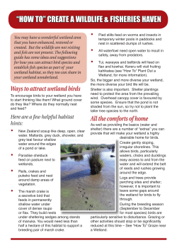


© Copyright 2026