
MANUAL FOR RAINBOW TROUT PRODUCTION ON THE
Nelson & Sons, Inc.
118 West 4800 South • Murray, Utah 84107
MANUAL
FOR RAINBOW
TROUT PRODUCTION
ON THE
FAMILY-OWNED FARM
by
GEORGE W. KLONTZ, M.S., D.V.M.
Professor of Aquaculture
Department of Fish and Wildlife Resources
University of Idaho
Moscow, Idaho 83843
Copyright 1991
All Rights Reserved
PDF file created by UC Davis/California Aquaculture, 6-00; JSC
This manual was prepared especially for Nelson and Sons, Inc., 118 West 4800 South,
Murray, Utah 84107, the manufacturers of Nelson's Sterling Silver Cup Fish Feeds.
TABLE OF CONTENTS
I. INTRODUCTION............................................................................... 4
A. Scope
B. Overview of the Process
II. FACTORS AFFECTING PRODUCTION .................................... 7
A. Fish-Associated
B. Water-Associated
C. Pond-Associated
D. Feed-Associated
E. Management-Associated
III. CONCEPTS OF PRODUCTION FORECASTING ................ 13
A. Product Definition
B. Carrying Capacities of Ponds
C. Production Plan
IV. CONCEPTS OF PRODUCTION METHODS .......................... 20
A. Pond Stocking
B. Pond Inventory
C. Growth Programming
V. PUTTING IT ALL TOGETHER ................................................... 28
A. Product Definition
B. Facility Description
C. Production Plan
D. Pond Stocking
E. Feeding Program
F. Inventory Data and Analysis
G. Conclusions
VI. COPING WITH DISEASE PROBLEMS ..................................... 34
A. Noninfectious Diseases
B. Infectious Diseases
VII. ECONOMICS AND MARKETING ............................................ 43
A. Production Costs
B. Marketing Techniques
VIII. BIBLIOGRAPHY............................................................................... 46
APPENDIX I: REFERENCE TABLES .................................................... 49
1. Weight-Length Values for Rainbow Trout
2. Dissolved Oxygen Concentrations at Saturation
3. Dissolved Oxygen Concentrations at 90 mm Hg P02
4. Percent Oxygen Saturation in Water at P02=90 mm Hg
5. Temperature-Related Growth Rates of Some Salmonids
6. Life Support Indices
7. Standard Metabolic Rates for Rainbow Trout
8. Dissolved Oxygen Recharge of Water Falling from Various
Heights
9. Feeding Chart for Trout
10. Unionized Ammonia Levels in Water
11. Julian Calendar
12. Weight and Measure Conversions
I. INTRODUCTION
A. Scope
This presentation is intended for the family-owned and -operated trout farm producing 15-50 tons
(30,000-100,000 lbs.) per year. The impetus for my writing this text comes from hearing genuine concerns about
rainbow trout in the marketplace. Chefs, restaurateurs, and retailers have stated quite clearly and repeatedly that they
expect farmed trout to be of high quality, delivered when needed, and presented in the form required. Stated another
way, quality, timeliness, and portion control are the bywords of successful trout production and marketing. Notice that
selling price is not among the concerns.
Unfortunately, the trout-producing community has yet to heed these concerns, if, indeed, they were even heard in
the first place. This is quite understandable, given the backgrounds of most family trout farmers and the availability of
these concerns to them. By and large, the family trout farmers are individuals who decided to produce trout because it
sounded like a good life and, in their enthusiasm, they learned how to raise trout. But then came the day of reckoning
-What do they do with their fish? Who will buy them? When will they buy them? In what form do they want to buy
them? Now the farmer has to become a processor, marketer, salesman, and merchandiser - all skills requiring more
knowledge than he/she possesses. At this point, trout farming becomes a whole new ballgame and survival is its name.
This treatise is designed to provide some insights on survival skills in trout farming.
The methods and suggestions offered in this text are compiled from methods used by trout farmers in many
countries. These farmers exemplify the saying, "Necessity is the mother of invention." The majority of the methods are
not published in any journal, and they have not been presented at association meetings. Most fish farmers seem to be
reluctant to share their experiences through these media. So, the best way to find out what is going on is to visit fish
farms and learn what is being done or not being done.
B. Overview of the Process
There are five major task groups which must be accomplished to produce a high quality trout product.
These are:
1. Establish a product definition.
2. Determine the capability of the farm to produce the product definition.
3. Develop a production plan.
4. Implement and monitor the production plan.
5. Market the fish.
4
Table 1
FACTORS AFFECTING THE PRODUCTION OF FARM-RAISED RAINBOW TROUT
A. Fish-Associated
1. Ammonia
2. Behavior
3. Nutritional requirements
4. Environmental requirements
a. Physical
b. Chemical
5. Product definition
6. Growth-rate potential
B. Water-Associated
1. Dissolved oxygen
2. Nitrite
3. Alkalinity
4. pH
5. Inflow rate
6. Suspended solids
7. Settleable solids
8. Temperature
9. Carrying capacity
10. Agricultural contaminants
11. Industrial contaminants
7. Disease history
8. Condition factor
9. Cannibalism
10. Oxygen uptake
11. Oxygen demand
12. Fecal solids
13. CO2
14. Stress response
12. Municipal contaminants
13. Natural contaminants
a. N2
b. CO2
c. H2S
d. Fe
14. Utilization
15. Salinity
16. Hardness (Ca++)
17. B.O.D.
18. Viscosity
C. Container-Associated
1. Water volume
2. Water velocity
3. Composition
4. Water-flow pattern
5. Water replacement time
6. Outfall design
7. Shape
D. Nutrition-Associated
1. Feeding rate
2. Feed efficiency
3. 3. Feed style
4. Nutritional quality
a. Proximate analysis
b. Energy content
5. Feed storage
E. Management-Associated
1. Fish sampling techniques
2. Feeding frequency
3. Feeding techniques
4. Record keeping
5. Pond cleaning
5
6. Fish-size grading
7. Management planning
8. Management objectives
9. Production economics
Figure 1
Interaction of biotic and abiotic factors in an aquaculture system
(Source: Downey, 1981)
6
II. FACTORS AFFECTING PRODUCTIVITY
Every trout farm, no matter how large or small, is composed of five major groups of factors which can, and often
do, affect the productivity of the farm. These are (1) the fish, (2) the water, (3) the pond, (4) the feed, and (5) the
management practices. Within each of these major groups are several individual factors, each acting in a mutually
interdependent fashion with other factors. (See Table 1 and Figure 2) That is, if one factor changes quantitatively, this
initiates a series of changes in several other factors. The net result can be beneficial to production or it can be
detrimental. It is incumbent upon the fish farmer to evaluate the initial change in terms of its possible end effect(s).
For example, the simple expedient of increasing the feeding rate, i.e., the lbs. of feed per 100 lbs. of fish, a
seemingly innocuous act sets into motion a series of quantitative changes within the system, which may or may not
result in achieving the desired result of having the fish grow faster. (See Figure 3)
In another example, the increase of water temperature from 9°C (48°F) to 15°C (59°F) generates the following
changes in the environment of a 100 gram rainbow trout:
A. Fish-associated changes
1. A 67.5% increase in metabolic rate (oxygen demand)
2. A 97.8% increase in daily length-gain potential
3. A 66.7% increase in daily weight-gain potential
4. A 98.6% increase in ammonia-generation potential
5. A 33.1% decrease in oxygen-carrying capacity
B. Water-associated changes
1. A 12.8% decrease in oxygen concentration
2. A 58.8% increase in environmental unionized ammonia
3. A 67.5% decrease in dissolved oxygen in the outfall water
Thus, the life support (oxygen-based) carrying capacity of the pond is greatly reduced, possibly to the point where
it could be detrimental to the health of the fish, depending upon the initial biomass in the pond. A method frequently
employed, where possible, to restore the oxygen-based carrying capacity is to increase the water inflow, which, in turn,
generates the following series of changes within the system:
1. The oxygen-based carrying capacity of the pond is increased
2. The water velocity is increased
3. The swimming energy expenditure of the fish is increased
4. The oxygen demand of the fish is increased
5. The oxygen-based carrying capacity of the pond is decreased
The net effect of these two alterations within the system might be mutually counterproductive to the physiological
status of the fish. A better solution to the reduction of oxygen-based carrying capacity might have been the reduction of
the population within the pond.
At this point, an in-depth examination of the specific factors is warranted:
A. Fish-Associated Factors
This group of factors can be termed intrinsic factors, in that they are part and parcel of the nature of the fish. Their
function is governed largely by the genetic make-up of the fish.
The major intrinsic factor affecting the well-being of the fish is the stress response. Fish in intensively
managed conditions are either continually or irregularly under the stressors of population density and
physical manipulations, i.e., grading, inventorying, pond cleaning, etc. The major physiological changes
7
5
occurring in the stress response that have the greatest impact on the health of the fish are the reduction of circulating
ascorbic acid (Vitamin C) and the increase in plasma cortisol. Both actions compromise the ability of the host to resist
the activation of a latent systemic bacterial or viral infection. Another aspect of the stress response is the induction of
environmental gill disease (EGD), which impedes the uptake of oxygen and the excretion of blood ammonia.
Other fish-associated factors, without regard to degree of significance, are:
1. Ammonia: As NH +4 , ammonia is generated in the system as the end-product of protein metabolism. There are
two major pathways of generation: endogenous and exogenous. The endogenous pathway is a catabolic function of the
body, in which the vital processes of the body are accommodated. The exogenous pathway is anabolic, in which the
dietary protein is metabolized for growth and other physiological functions. The fish excretes ammonia, as NH +4 , across
the gill membranes. In the aquatic environment the measured ammonia occurs in two forms: dissociated or ionized
( NH +4 ), which is nontoxic for fish, and undissociated or unionized (NH3), which is toxic for most finfish at continuous
levels exceeding 0.03 mg/1. The ratio of NH +4 to NH3 is both temperature- and pH-dependent. (See Appendix I: Table
10)
2. Behavior: Rainbow trout are territorial animals. When in free-living or confined conditions they establish their
required amount of space based upon water conditions and food availability. They will defend these areas quite actively.
In confined conditions, the defensive acts are mostly in the form of nipping the dorsal fin and/or pectoral fins of the
transgressor. This gives rise to the injured areas appearing as a "target" to other aggressive fish in the population. The
fin-nipping sometimes becomes so severe that the condition called "soreback" occurs. Thus, it is desirable to have
ponds and pond loadings so as to permit the establishment and maintenance of territories. It is then incumbent upon
the fish farmer to feed the fish so that a fish does not have to "invade" the territory of another to acquire food.
3. Nutritional Requirements: Based upon their food preferences, rainbows are carnivores. Thus, it follows that the
dietary formulation must satisfy this need. The current state of knowledge about fish nutrition is such that nutritionally
adequate diets are available for most species of salmonids.
The energy ingredients of a trout diet formulation are protein, lipid (fat), and carbohydrate. The protein comes from
both animal (fish meal) and plant (wheat, corn, soybean) sources. The lipid comes from fish meal and fish oil. The
carbohydrate comes from the ingredients of plant origin.
Rainbow trout require 1600-1650 metabolizable kilocalories (kcal) of energy per lb. of weight gain. They can derive
4.0 kcal per gram of digestible crude protein, 9.0 kcal per gram of digestible lipid, and 1.8 kcal per gram of digestible
carbohydrate. The majority of commercial fish feeds are designed energy-wise to provide feed conversions of 1.2-1.4:1.
The Silver Cup formulation typically delivers a feed conversion of 1.2:1, if properly fed.
4. Environmental Requirements: Rainbow trout are classified as cold-water fish as their Standard Environmental
Temperature (SET) is 15°C (59°F). For each degree C above or below the SET, there is an 8.5% reduction in metabolic
rate, which can be translated into a comparable decrease in weight gain or growth.
Other environmental preferences are dissolved oxygen levels above 60% of saturation and continuous levels of
ammonia (as NH3) below 0.03 mg/l. These are "No-Effect Limits" (NEL). The NEL values for other environmental
requirements are presented in Table 2.
5. Product Definition: This term is a relatively new concept to intensive aquaculture. It implies that the production
cycle begins with the size and number of fish to be harvested on or about a specific date. The process then proceeds
backwards in time, taking into account the several factors which might influence production, and identifying a starting
date and the management processes which must be implemented to achieve the Product Definition.
8
Figure 2
The effects of increasing the feeding rate to a group
of rainbow trout (Source: Klontz, et al, 1989)
6. Growth Rate Potential (GRP): Growth of rainbow trout can be measured as an increase in length, weight, or both.
The GRP is largely under genetic control and influenced by water temperature (Appendix I: Table 5).
The Allowable Growth Rate (AGR), on the other hand, is the growth rate which the system will permit. The major
factors which affect the AGR are:
a. Water temperature
b. Oxygen availability
c. Water osmolarity
d. Feed quality
e. Feed quantity
f. Subclinical respiratory disease
Under ideal conditions, the AGR and the GRP are equal; however, in the majority of cases this is not the case. Plus,
an aquaculturist should be capable of taking all the factors influencing growth into consideration to establish the AGR of
the system. The AGR then becomes the key factor in production forecasting to achieve the Product Definition.
7. Disease History: The impacts of clinical and subclinical episodes of infectious and noninfectious diseases on
productivity have been documented. However, the documentation relates more to the impact of dead fish rather than
those that are clinically ill but do not die. When fish are exposed to environmental
9
conditions that exceed the accepted "No-Effect Limits" for an extended period, there comes a point where the fish can
no longer cope with the situation. Two of the first signs of this are the loss of tissue between the fin rays (the "frayed
fin" syndrome) and a generalized melanosis (body darkening).
8. Length-Weight Relationship: This factor - called the "condition factor" - is, perhaps, the most misused mathematical
term in aquaculture. Typically, populations are inventoried periodically for growth and feed conversion. This process
entails the weighing of groups (sample lots) of fish to obtain the number of fish per pound - or a reasonable estimate
thereof. This statistic is then used to determine the mean length of the fish using a weight-length table (Appendix I:
Table 1). Unfortunately, most tables assume a constant condition factor which is not true - thus, an incorrect length is
obtained, which then leads to further complications because the feeding rate models use body length as their basis.
If condition factor is to be used in the production process, as it should be, then individual fish must be weighed and
measured at the end of each growth stanza or period and the condition factor calculated from these data.
9. Cannibalism: The major impact of this factor is having a progressive loss of small fish in the fish
population, which can lead to errors in estimating biomass. The problem can be circumvented by (1) grading
and/or (2) feeding regimen. With respect to the latter, if populations are fed in such a fashion, i.e., hand
Table 2
THE "NO-EFFECT" PHYSICAL AND CHEMICAL LIMITS
OF WATER SUPPORTING MOST FINFISHES
PARAMETER
Dissolved oxygen
pH
Alkalinity
Carbon dioxide
Calcium
Zinc
Copper
Iron
Ammonia-N (as NH3)
Nitrite-N
Nitrogen
Suspended solids
Dissolved solids
Temperature
10
VALUE
> 90 mm Hg p02
ca. 60% of saturation
6.7-8.5
30-200 mg/I as CaC03
<2.0 mg/1
>50 mg/1
<0.04 mg/1 at pH 7.5
<0.006 mg/1 in soft water
<0.3 mg/l in hard water
< 1.0 mg/1
<0.03 mg/1 constant
<0.05 mg/1 intermittent
<0.55 mg/I
< 100% of saturation
<80 mg/1
50-200 mg/1
SET for species
feeding, that the size variance is minimal, then cannibalism is minimized. This, plus judicious grading, will nearly always
preclude cannibalism from being a serious problem.
10. Oxygen Uptake: The rate of oxygen uptake across the gill lamellar membranes is a function of the differences in
partial pressures of dissolved oxygen between the water and the lamellar capillaries. Under ideal conditions, the partial
pressure difference should be 15-20 mm Hg. However, if the gill lamellar epithelia become hypertrophic or hyperplastic,
the p02 difference must be greater. If the p02 difference is insufficient, the oxygen demand of the fish cannot be met and
growth suffers accordingly.
11. Oxygen Demand: The oxygen demand of fish is regulated by the metabolic rate. The Standard Metabolic Rate
(SMR) is influenced by water temperature, primarily, and age (as fish size), secondarily (Appendix I: Table 7). If the
oxygen demand cannot be met because of insufficient p02 differential between the water and the lamellar capillaries, the
metabolic rate is negatively influenced, which, in turn, negatively influences the growth rate and the general well-being of
the fish.
12. Fecal Solids: The resultant influence of fecal solids on productivity is, if they are left to accumulate, a reduction in
growth rate. This can occur via one or more of the following changes in the system, attributable to the presence of fecal
solids.
a. Increased Biological Oxygen Demand (BOD)
b. Sestonosis - an accumulation of solids and other detritus on the buccal aspect of the gill rakers
c. Lamellar thickening (hypertrophy or hyperplasia) resulting from the physical irritation due to solids passing
over the lamellar tissues
d. Toxic by-products of fecal solid decomposition
13. Carbon Dioxide: Fish-generated carbon dioxide is a respiratory by-product. Other than in closed, recycled water
systems, it should have no deleterious effects. On the other hand, plasma carbon dioxide levels can influence the
off-loading of oxygen from hemoglobin at the tissue level. This can adversely affect the productivity.
B. Water-Associated Factors
The productivity of an aquaculture facility is largely dependent upon the quality and quantity of water available. The
container, nutrition, and management factors are subordinate to the water quality and quantity. The factors to be
identified and defined all must be considered as equally important to productivity.
1. Dissolved Oxygen: To be within the accepted "No-Effect Limits" for most species of salmonids, the dissolved
oxygen in the water entering the facility should be >95% of saturation (Appendix I: Table 2). The dissolved oxygen in
the water exiting a rearing unit should have a p02 of >90 mm Hg (Appendix I: Table 3). This is a departure from the
traditionally accepted dissolved oxygen limit of 5 mg/l, which under certain circumstances of temperature is less than 90
mm Hg pO2.
2. Nitrite: Nitrite is the oxidation product of ammonia-nitrogen. It is under the influence of Nitrosomonas sp. The
accepted tolerance level of nitrite is 0.55 mg/1. Levels exceeding this create methemoglobinemia, in which the iron in the
heme molecule becomes reduced and cannot transport oxygen, thus inhibiting the satisfaction of the oxygen demand of
the fish.
3.Alkalinity and Hardness: In freshwater systems, fish are hypertonic to their environment. That is, water is attempting
to equilibrate the differences in osmolarity; thus the fish must excrete large quantities of urine to maintain its internal
physiological balance. Fish in marine environments are hypotonic to the environment and must drink water to maintain
their physiological balance. Thus, in freshwater situations, fish in hard
11
water (>250 mg/1 alkalinity) will spend less metabolic energy on osmoregulation than fish in soft water (<100 mg/1
alkalinity), thus providing more metabolic energy for growth.
4. Contaminants: Waters used in aquaculture systems must be virtually free of municipal, industrial, and agricultural
contaminants. In addition, natural contaminants, such as heavy metals (Cd, Cu, Zn, and Hg) must all be in the <0.1
mg/1 range. One of the major natural contaminants is nitrogen supersaturation of the water. Excesses above 100% of
saturation will create "gas-bubble" disease, a syndrome in which nitrogen comes out of solution in the plasma and creates
gas emboli that interfere with blood flow to organs and tissues. Many water sources, especially those from deep wells, are
oxygen deficient and supersaturated with nitrogen. In these cases, the best remedy is to pass the water through packed
columns for gas stabilization prior to use in a rearing unit.
5. Solids: Waters containing high levels of certain types of suspended/settleable solids can create impairment of
oxygen uptake by causing an inflammatory response in the gill lamellar tissues. In addition, certain plant pollens
(especially pine pollen) can cause similar problems in gill tissues. The net results are often a reduction of growth rate and
an increase in feed-conversion ratio.
C. Container-Associated Factors
This group of factors which can affect productivity is largely hydraulic in nature. The water replacement time and
the water velocity function to provide adequate available dissolved oxygen for the fish and to remove the potentially
deleterious metabolic waste products.
D. Nutrition-Associated Factors
As has been stated, adequate nutrition is a key factor to optimizing growth and product quality. The diets must be
formulated and presented with the requirements of the fish in mind. If these requirements are not met, the production
goals will be compromised accordingly. It should be reiterated that this aspect of aquaculture technology is the most
expensive in terms of production costs. It is also one aspect - if not the main aspect - over which the aquaculturist can
exercise control. The other groups of factors - save the management-associated factors -cannot be altered routinely or
easily. Their influence constitutes the nature of establishing the Allowable Growth Rate (AGR), i.e., the growth rate that
the system will permit.
E. Management-Associated Factors
This group of factors comprises the discretionary activities that an aquaculturist can exercise during the production
cycle. Each must be executed after giving some consideration to the possible effects of such activity on production. For
example, increasing the feeding rate to a population of fish would ostensibly result in an increase in growth rate - but only
if done within the limits imposed by the system. There are at least three other metabolic pathways that could negatively
impact growth rate and offset the anticipated increase in productivity (Figure 2).
12
III. CONCEPTS OF PRODUCTION FORECASTING
Production forecasting is the application of techniques to prepare a production schedule for market-size rainbow
trout. The process might seem somewhat complicated at first, but, with time and patience, the benefits of this approach
should become apparent in terms of numbers and quality of fish produced and reduced production costs.
The process follows a logical sequence of activities. First, the trout farmer must decide on a Product Definition.
Next, he or she must determine whether or not the facility can produce that fish in that quantity - thus, the carrying
capacities of the farm must be defined. Finally, the production plan is developed, implemented, and evaluated. Each step
must be accomplished in sequence if the process is to be beneficial. So, without further ado ....
A. Product Definition
The production-forecasting process begins with establishing the Product Definition. This embodies designating the
following product criteria:
1. Species (strain) of fish to be produced
2. The average size of fish to be harvested (g/fish; oz./fish; no./lb.) (round weight or dressed weight) 3. The
number of fish to be produced
4. The biomass (lbs.) to be produced
5. The date(s) of harvest
A Product Definition for a rainbow trout should be based upon the nature of the product appearing in the
marketplace (Table 3).
An example of an acceptable Product Definition would be:
2,500 rainbow trout (Kamloops) at 1.42-1.19/lb. (320-380 g/fish) (round weight), (250-300 g
dressed weight) are to be harvested weekly for processing.
B. Carrying Capacities of Ponds
The concepts of carrying capacities or rearing ponds bring together the interaction of the fish with the aquatic
medium, the fish with the rearing unit, and the aquatic medium with the rearing unit. Stated in other terms, the carrying
capacity concepts are the balance of the biotic (fish) factors with the abiotic (water and pond) factors. The fish are the
key issue in these concepts. For optimum performance (growth, health, and feed conversion), the needs of the fish
relative to rearing space, life support (dissolved oxygen), and water quality must be met. There are four fundamental
carrying capacity concepts in intensive aquaculture, namely, (1) density, (2) oxygen, (3) ammonia, and (4) suspended
solids.
It should be noted that the fish will (should) not suffer irreparable harm if one or more the carrying capacity values
are exceeded, but their performance, i.e., growth rate and feed conversion, will be compromised to a measurable degree.
The negative effects on productivity are dose-dependent, i.e., the more one of the carrying capacity limits is exceeded,
the greater the effect on the fish.
Each carrying capacity has its unique set of determinant factors (Table 4). As such, each must be defined for each
rearing unit and/or system. The lowest value becomes the maximum permissible biomass of a specified species. At this
point in time, virtually all of the methods used to estimate carrying capacities are applicable only to salmonids.
1. Required data: The process of determining the carrying capacities of each rearing unit begins with collecting and
recording the necessary data. The following data must be collected with precision if the concepts of carrying capacities
are to be implemented with any degree of reliability:
13
Table 3
PROCESSED PRODUCTS OF RAINBOW TROUT AVAILABLE
IN THE MARKETPLACE IN AMERICA AND WESTERN EUROPE
TRADITIONAL
Iced - round dressed
boned fillets
Frozen -
dressed
boned
boned and breaded
boned and stuffed
boned fillets
VALUE-ADDED
Smoked - dressed
boned
fillets
sausage
roll
Kippered – dressed
fillets
boned
Soup - creamed
Vol-au-vents
Toast toppers
Canned –minced
whole
pate
quiche
paste
crepes
mousse
kedgeree
"burger"
hoagie
goulash
pancakes
pickled fillets
pet food
a. Physical parameters
1) Pond dimensions – total water dimensions (ft.)
– total fish rearing dimensions (ft.)
2) Water use
– single-pass system
– mutable pass
• number of falls between uses
• height of each fall (ft.)
3) Elevation of the farm above sea level (ft. above MSL)
4) Daily mean water temperature (weekly basis) (ºC)
5) Water inflow (gpm, cfs, lps, lpm, or cms)
b. Chemical parameters
pH
Alkalinity (mg/l)
Dissolved nitrogen (% sat.)
Dissolved oxygen (mg/l)
Unionized ammonia (mg/l)
Nitrate (mg/l)
14
Calcium hardness (mg/l)
Specific conductance (umos)
Biological Oxygen Demand (mg/l)
Total ammonia (mg/l)
Nitrite (mg/l)
Total phosphate (mg/l)
Table 4
CARRYING CAPACITY DETERMINANT FACTORS
CARRYING
CAPACITY
DETERMINANT
FACTORS
Density
Rearing Space
Fish length
Water temperature
Elevation
Water inflow to pond
Standard Metabolic Rate
Water temperature
Water pH
Feeding rate
Protein content
Protein digestibility
Feeding rate
Feed digestibility
Water-retention time
Water velocity
Oxygen
Ammonia
Solids
c. Water discharge permit specifications – ammonia
– solids
• suspended
• settleable
– phosphate
d. Feed quality
– metabolizable energy (kcal/lb.)
– protein content (%)
– estimate feed conversion ratio
2. Density-carrying capacity: The density-carrying capacity of a pond is based upon the spatial requirements for the fish
in the system (Piper, et al, 1982). The formula is:
Wden=Pvol*Dfac
When: Wden=biomass (lbs.) of fish per unit of body length (in.) per pond
Pvol=pond volume (cu. ft.)
Dfac=density index (lbs. fish per cu. ft. or rearing space per in. of body length)
Species
lb./in./ft.3
RBT-Shasta
RBT-Kamloop
Steelhead
Chinook salmon
Coho salmon
Atlantic salmon
0.5
0.5
0.25
0.3
0.4
0.3
15
To determine the density-based permissible biomass in the rearing unit, the following formula is applied:
Bio=Wden*L
When: Bio=permissible biomass (lbs.) based upon the density-carrying capacity
Wden=biomass (lbs.) per unit of mean body length (in.) for the rearing unit
L=the mean body length (in.) of the fish in the target population
4. Oxygen-carrying capacity: The oxygen-carrying capacity of a rearing unit may be estimated using one of several
methods. Each has its unique application and limitations.
a. Single-Pass System
To calculate permissible oxygen-based biomass (lbs.) in a single-pass, open water system, the following formula may
be used (Piper, et al, 1982):
W=F*L*I
When: W=permissible biomass (lbs.) of fish at length L
F=lbs. fish/gpm/in. body length (from Appendix I: Table 6)
L=mean body length (in.)
I=water inflow (gpm)
This method is applicable only to single-pass, linear rearing units. The F-value is based upon the temperature and
elevation-compensated oxygen requirement of the fish per unit of body length. Implicit within the value is an
inflow-dissolved oxygen level of >95% saturation and an outfall-dissolved oxygen level of 5.0 mg/1. Thus, unless there
is sufficient oxygen recharge between uses, the fish in successive uses will be in an oxygen-deficient medium.
b. Multiple-Pass Systems Without Supplemental Aeration
Ponds, particularly raceway ponds, arranged for serial passage of water have been one of the more serious
constraints to successful fish health management. In systems utilizing 3-5 serial water uses, the status of health in
succeeding populations often gets progressively worse. This condition is influenced by at least three major factors within
the system: 1. The size of fish. 2. The successive accumulation of waste products (fecal material and ammonia) and
uneaten food. 3. The successive depletion of dissolved oxygen. Thus, any successful production in situations such as this
must take these three constraints into account.
First, the anticipated dissolved-oxygen depletion must be defined. By way of example, the system to be modeled is a
series of five raceways (10' wide, 100' long, 3' water depth) at a 1,000 foot elevation. Between each raceway in the series is
a 3' fall, which serves to recharge the water with dissolved oxygen. The water inflow to the first-use pond is 2.0 cfs (56.64
lps). The water temperature is 15°C (59°F). The dissolved oxygen content of the water at 95% saturation is 9.71 mg/1
(Appendix I: Table 2). Thus, there is a total of 1,979,907.8 mg dissolved oxygen entering the pond per hour.
There should not be more than a 30% depletion of total dissolved oxygen in the first use. Thus, the water exiting the
first-use pond should be 70% of saturation (6.8 mg/1). With the fall from the first-use pond into the second-use pond,
there will be an oxygen recharge to 82.59% of saturation (8.02 mg/1) (Appendix I: Table 8). The water leaving the
second-use pond should have a partial pressure of oxygen (POD of not less than 90 mm Hg or 59.75% of saturation (5.8
mg/I) (Appendix 1: Table 3). With the fall between the second-use and the third-use, the oxygen saturation of the water
entering the third-use pond will be 76.2% (7.4 mg/1). Again, as with the second-use pond, the water exiting the third-use
pond should not be less than 59.75% of oxygen saturation. The fourth and successive passages of water will be the same.
Now the system has been "stabilized" with respect to available dissolved oxygen.
There will be 2.91 mg/I D.O. available in the first use, 2.2 mg/1 D.O. available in the second use, and ca. 1.6 mg/1
available in the subsequent uses in the system. Expanding these data to oxygen availability per hour in each pond, the first
pond will have 593,972.3 mg, the second pond will have 448,588.8 mg, the third and successive ponds will have ca.
326,246.4 mg.
16
The next step is to determine the oxygen utilization (mg/hr) by rainbow trout of a specific size. This can
be accomplished using the Standard Metabolic Rate table (Appendix I: Table 7).
With the oxygen requirement of the fish known, this value divided into the amount of oxygen available
in each pond generates the permissible head-count. The head-count divided by the number of fish per kg or
lb. generates the permissible biomass.
c. Multiple-Pass Systems With Supplemental Aeration
Providing multiple-pass systems with supplemental aeration may be accomplished by providing either
pumped air or pure oxygen (as a gas or a liquid) into either the inflow end of each successive raceway or
throughout the length of each raceway. In such cases, if the supplemental oxygenation is sufficient to have the
dissolved oxygen in the pond outfall water >60% of saturation, the density-carrying capacity becomes
limiting.
With any form of supplemental aeration, there is always the risk of supersaturating the environment with
nitrogen (in the case of using pumped air) or oxygen (in the case of using gaseous oxygen). The nitrogen
supersaturation can cause acute gas-bubble disease at levels exceeding 110% of saturation and chronic
gasbubble disease at levels exceeding 102%. The oxygen supersaturation below 2 atm of pressure is not likely
to cause health problems for the fish.
The most efficient and safe method of introducing pumped air into a fish-rearing unit is via gas
stabilization chambers, rather than by a venturi or airstones. In any event, the total gas pressure should not
exceed 100% of saturation, to preclude any unwanted health problems for the fish.
d. Circulating Water Systems
The oxygen-carrying capacities of circulating water systems, i.e., circular or rectangular circulating ponds,
by virtue of their hydraulics, cannot be calculated using the methods described for linear or noncirculating
water systems. In circulating water systems, there is a considerable degree of homogenization of the inflow
water with the water already in the system.
If there is no supplemental aeration, the most reliable method of estimating the oxygen-carrying capacity
in these systems is by monitoring the system as the biomass increases. The outfall-dissolved oxygen level is
established at the mg/1 or percentage of saturation when the p02 is 90 mm Hg. Daily dissolved-oxygen levels
in the outfall water are measured. When the dissolved-oxygen levels are near or below the set values, the
biomass and size of fish are recorded for future pond-loading criteria.
Circulating water systems are becoming more and more frequently employed because they are less
consumptive of water than are linear, noncirculating systems. The reduced water use virtually mandates the
use of supplemental aeration. Thus, if the system is properly aerated, it removes the dependency of the fish on
dissolved oxygen, and the limiting carrying capacity is the density. The supplemental aeration of circulating
systems has the same attendant caveats as in the linear, multiple-pass system.
5. Ammonia-Canying Capacity: The ammonia, as NH3, carrying capacity is based upon the Median Tolerance
Limit - Chronic (TLMc) of unionized ammonia (NH3) by salmonids. The currently accepted TLMc value for
salmonids is constant exposure to <0.03 mg/1 NH3 or intermittent exposure to <0.05 mg/I NH3. The pH
and temperature of the water directly influences the degree of free ammonia (as NH3) generated (Appendix 1:
Table 10).
There are several methods of estimating ammonia production in fish-rearing units. The method of Meade
(1974) provides a relatively simple and reliable estimate of total ammonia generated by salmonids.
The formula is:
17
Pa=Rf * W * Nl * Nu * Ne
When: Pa = total ammonia (kg) generated daily
Rf = daily feeding rate (kg/100 kg biomass)
W = biomass (kg)
Nl = protein content of diet (%)
Nu = protein digestibility (%)=0.9
Ne = nitrogen (%) excreted as ammonia-N=1.0
In properly managed, single-pass linear systems, the ammonia-carrying capacity should not be exceeded. However,
in multiple-pass systems, the risk of exceeding the limit of 0.03 mg/1 can occur because of the increased accumulations
with each successive reuse of the water. The same can occur in circulating systems by virtue of an increased
water-retention time. In both cases, the problem can be alleviated by reducing the feeding intensity (rate).
6. Suspended solids-carrying capacity: As with the methods of estimating the amount of ammonia generated, the methods
of estimating the amounts of fecal solids are quite unreliable. There are at least two major dependencies, namely, the
digestibility of the feed (feed conversion ratio) and the feeding techniques. The tolerance limits of salmonids for
suspended solids, although quite broad, also depend upon the nature of the solids, i.e., are they gill tissue irritants or not.
Most fecal and uneaten feed solids are quite nonirritating to salmonids larger than 40/pound. Smaller fish can accumulate
solids on the buccal ("upstream") aspect of their gill rakers. These solids become conducive to the growth of aquatic
fungi, which further blocks the water-flow over the gills and reduces oxygenation of the fish. This condition is termed
sestonosis and there is no treatment for it.
C. Production Plan
Beginning with the time period for harvesting the fish, the next step is to calculate the time required to have fish of
the specified size. That is, the water temperature-dependent growth rate must be established on a growth period basis.
The length of a growth period in most instances is 14 days; however, longer periods have been used. One caveat in this
is that the longer the period, the greater the error, because of having to use a mean water temperature and a constant
condition factor for an extended period. The suggested approach is to use 14-day intervals for the programming
segment. Another suggestion is to use a Julian date calendar (Appendix I: Table 11) in conjunction with the usual
calendar dating.
The format for generating a production plan contains 8 categories (Figure 3):
1. Date
2. Mean daily water temperature (°C)
3. Number of fish
4. Mean body length (mm)
5. Mean weight per fish (no./lb.)
6. Biomass (lbs.)
7. Weight gain (lbs.) during the period
8. Feed required (lbs.) during the period
The first task is to complete the dating sequences and mean daily water temperatures in 14-day intervals, beginning
with the harvest date and working backward in time for what would be estimated as the time required to produce this
fish. The second task is to complete the number of fish column, beginning with the harvest number and increasing this
number by the anticipated mortality during each 14-day period. The usual daily mortality is calculated at 0.02%. It is not
advisable to estimate the mortality expected to occur due to disease episodes.
The temperature-dependent expected body-length increases are estimated using the data in Appendix I: Table 5.
18
The weight-per-fish data are obtained from either historical data or from the weight-length table (Appendix I: Table
1). The weight-per-fish values are multiplied by the headcount data to calculate the biomass (lbs.).
Date
Water
Temp.
(°C)
Number
of Fish
Mean
Length
(mm)
Mean
Weight
(n/lb.)
Total
Weight
(Ibs.)
Weight
Gain
(Ibs.)
Feed
Req'd.
(lbs.)
Figure 3
Example of a format for production planning
The feed requirements on a growth-period basis can be calculated, as follows:
dW = Bend - Bbeg
When: dW = weight gain (lbs.) during the growth period
Bend = biomass (lbs.) at the end of the growth period
Bbeg = biomass (lbs.) at the beginning of the growth period
Ffed=dW*FCR
When: Ffed=amount of food required (lbs.) during the growth period
dW=weight gain (Ibs.) during the growth period
PCR=estimated food conversion ratio
This sequence is continued backwards in time until the fish are of a size to be well on feed -- usually 10001b. for the
time required to begin the production from either green or eyed eggs, a thermal (temperature) unit chart should be
consulted (Piper, et al, 1982).
19
IV. CONCEPTS OF PRODUCTION METHODS
A. Pond Loading
In many of today's finfish-production facilities, fish are often stocked into rearing ponds quite arbitrarily - sort of by
the "seat of the pants" or "it looks about right" method. These fish are fed daily and, perhaps, evaluated for growth and
feed conversion on a biweekly or monthly basis. When the pond "looks a bit overloaded," the population is reduced by
grading or general transfer to another pond.
An alternative to the foregoing scenario is the practice of "stocking the pond for take-out." This means that the
pond is stocked with the number of fish (plus ensuing mortality) that are to be removed some weeks or months from the
stocking date. The process is quite simple, namely:
1. Establish the date on which the pond population is to be reduced by grading or random transfer to
another pond.
2. Determine the number of growing days between the date of stocking the pond and the date of
population reduction.
3. Calculate the temperature-based daily growth rate (mm) of the fish between the pondstocking date
and the population-reduction date (Appendix I: Table 4).
4. Apply the daily length-increase data on a day-by-day fashion throughout the period between pond
stocking and population reduction.
5.
Using the weight-length table, determine the number of fish per lb. (Appendix I: Table 1).
6. Determine the permissible biomass (lbs.) based upon the lowest carrying capacity parameter.
7. Determine the permissible number of fish by multiplying the biomass by the number of fish per lb.
8. Estimate the "natural" mortality to occur between the dates of stocking and population reduction. A
reliable figure to use is 0.02-0.03% per day. DO NOT ANTICIPATE DISEASE EPISODES!
9. The sum of the permissible number at the end of the growing period and the accumulated daily
mortality generates the number of fish to be stocked into the pond. This number, divided by the
number of fish per lb. on the date of stocking, generates the biomass to be stocked into the pond.
From the point of pond stocking, good husbandry is the watchword. The fish are fed, ponds are cleaned, feeding
and inventory records are kept, and all should be well.
B. Pond Inventorying
Anyone who has dealt with raising fish under intensively managed conditions knows first-hand the frustration of not
knowing with any degree of certainty either the exact number or biomass of fish in a given pond population. Most fish
farmers would agree that +/- 5% discrepancy between what is actually in the pond and what the record book indicates
would be acceptable. However, the discrepancy is quite often in the neighborhood of +/-15-25%. This makes growth
programming quite difficult and frustrating. The sources of the error, most would agree, is in the acquisition of pond
inventory data, the unaccountable numbers of fish escaping, eaten by birds and eaten by their pond-mates, and in the
recording of the daily mortality. (The prioritization of these sources of error is mine, not the industry's).
The basic purpose of a regularly scheduled population inventory is to determine the following statistics:
1. Growth, as increases in individual length and weight, and in population weight
2. Feed conversion
20
3. Other factors costs of production
mortality (daily rate and total size variations within the population)
percentage of pond-carrying capacity being used
To determine these statistics, ideally, the following performance indicators should be measured:
1. Mean length increase (mm)
2. Mean body weight increase (lbs.; g; no./lb.)
3. Biomass increase (lbs.)
4. Condition factor change
5. Length variation within the population
a. Median
b. Mean
c. Mid-range
d. Standard deviation
e. Coefficient of variance
6. Body weight variation within the population
a. Median
b. Mean
c. Mid-range
d. Standard deviation
e. Coefficient of variance
7. Feed conversion ratio
8. Dress-out percentage
9. Depuration weight loss (%)
10. Gross appearance
11. Flesh quality
Obviously, the best method to acquire the data to quantify the listed evaluative criteria would be to count and
weigh the entire population. In practice, however, this is not very realistic because of the time and labor requirements.
Therefore, the next approach is to have reliable sampling methods, of which there are many.
Basically, there are three methods, each with several variants, by which to sample pond populations. First, a few
handfuls of feed are cast out into ponds, and when there is a feeding "boil" a cast net is thrown over it. The collected fish
are weighed, usually in the net, and counted back into the pond. The weight, minus the weight of the castnet and number
of fish, is recorded. This process is repeated three or four times at different sites in the pond. The data are handled either
(1) by totaling the numbers of fish and the sample weights and calculating the mean number of fish per pound or (2) by
determining the number of fish per pound for each sample and determining the mean number of fish per pound from
that.
The latter method does have the advantage of indicating the variation in fish size, whereas the former does not. But,
statistically, it is not sound because it is calculating a mean value from a series of mean values. The main sampling error
encountered in this technique is that most often the only "lead" fish in the population are sampled. If the growth
program can account for this bias, then the validity of the technique is increased. The main advantage of the technique is
that it requires only one person and very little time.
The second and, perhaps, the most common technique is, after 18-24 hours of feed deprivation, to crowd the fish
to one end of the pond and to take several samples for weighing and counting. This method does reduce the bias of
sampling only a small segment of the population. And, if performed well, the results can be quite illustrative of the actual
population composition. The major drawbacks to this procedure are (1) the personnel and time commitments and (2) the
stressful nature of the technique. There have been innumerable references to this method being "the best diagnostic tool
for ERM or IHN."
The third technique (the "5x5" method) is much like the second in that the 18-24-hour post-prandial
(since eating) population is crowded into a small space. The degree of crowding should be such that in a 3-
21
foot water depth the bottom of the crowding screen is not occluded by the fish density. Of course, this presumes that
the water clarity is such that it permits this. If it is not, then one will have to make a "judgment call." Just outside the
area of crowding is a live box (ca. 3'x3'x3') (Figure 5). Five nets of fish are dipped from the crowded population into
the live box. One net of fish is removed, the fish weighed and counted, and returned to the area outside the crowded
area. The live box is emptied (tip it over). This process is repeated five times. During the process, one or two of the
samples of fish to be weighed and measured are anesthetized. At least 40 of the group are selected at random for
individual lengths (mm) and, if possible, weight (g). This entire process requires no more personnel or time than does
the second method — but there is greater attention to detail.
Figure 4
Schematic of activities for the "5-by-5" method of pond inventorying
The "5-by-5" method does have the following advantages over the other two, namely:
1. The following length-weight characteristics of the population are recorded:
a. Length frequency
b. Weight frequency
c. Mean individual length
d. Mean individual weight
e. Range, mid-range and median values for length and weight
f. Number per unit of biomass
22
2. From the foregoing, an assessment of the need to grade the population can be made. The usual criterion is at
point when the length of the shortest fish in the population is less than 50% of that of the longest fish.
3. By using graphic plots of the length and weight data, the sizes for grading can be determined.
4. The estimations of weight gain, length increase, and feed conversions are made significantly more reliable.
Once again, the decision of which of several methods to use to accomplish some action in fish health management
must be made. In my opinion, given the nature of intensively managed fish farms, the best inventory method is a
combination of all three of the methods described. Each has its particular place in the scheme of things and, as such, can
be quite useful. A typical scenario would be:
1. After determining as accurately as possible the number of fish per unit of weight (preferably n/Ib.), weigh the
prescribed biomass of fish into the pond.
NB: The following approach to weighing groups of fish into a pond is suggested:
a. Groups of small fish (40-75 mm) should be weighed +/- 1.0 g.
b. Groups of fish 75-150 mm should be weighed +/- 5 g.
c. Fish over 150 mm should be weighed +/- 10 g.
Rationale: 1 g =1/454th of a pound
10 g =1.45th of a pound
1 oz.=1/16th of a pound (28.38 g)
Thus, the opportunity for rounding error is much less with the metric system than with the avoirdupois
(American) system.
2. The first inventory of a pond population (fish over 100 mm) should be done as follows:
a. Sample as in Method 1 (the castnet method), with the following modification: anesthetize, weigh and measure
at least 40 fish in each sample. This will indicate which portion of the population is sampled by this technique.
b. Sample as in Method 2 using the modification listed above for the same reason.
c. Sample as in Method 3 to establish the population-size composition.
d. Evaluate all data in terms of their conformity with each other and with their unique portions of
the population sampled.
3. The next series of inventories (4-5) can be done using Method 1. Remember, the growth-programming data for
feeding rates must be adjusted accordingly. If in doubt, then the best suggestion is to go back to the pond with Method
3. With a little practice, one should be able to use this approach quite reliably.
4. At intervals, especially prior to grading the population, it is suggested that Method 3 be used in addition to
Method 1. At this point, the population-size composition should be as accurate as possible.
The collected length and weight data are recorded (Figure 5) for later comparison with the expected length and
weight data. If the feeding program for the previous growth period was effective, there should be very little difference
between the inventory (observed) data and the expected growth data. If, however, the differences are greater than S%,
then some adjustments must be made for the upcoming growth period.
C. Growth Programming
There are several methods by which feeding rates may be calculated. None is actually better than the
other. The best basis for selecting a feeding-rate calculation method is its degree of suitability to the system.
23
Pond No:
Date:
Sample
Number
Weight
(g)
Number
(lb)
Length: Weight — Individual Fish
mm
g
mm
g
mm
g
mm
1
1
1
1
2
2
2
2
3
3
3
3
4
4
4
4
5
5
5
5
6
6
6
6
7
7
7
7
8
8
8
8
9
9
9
9
10
10
10
10
g
Figure 5
Example of an inventory data recording form
Of all the methods to derive feeding rates for fish, the Haskell method has been used the most widely.
The equation is:
Rf=(dL*FCR*3 * 100)/Ld
When: Rf = lbs. of feed per 100 lbs. of fish daily
dL = daily length increase (in.)
FCR = feed conversion ratio
3 = length-weight-conversion factor
100 = decimal-removing factor
Ld = length (in.) of fish on the day of feeding
The first step applying this model to a group of fish is to establish the length of the growth period. In
practice, a 14-day growth period has been found to be most reliable. However, periods of up to 28 days have
24
been used. The major reason for suggesting the 14-day period is to reduce the error created by the increasing condition
factor. In the example following, a 14-day feeding period is used (Figure 7). The feeding on Day 1 uses an Ld value
derived from an inventory. On Day 2 the Ld value is increased by the dL. On Day 3 the Ld value is the original Ld value
plus 2 dL values, and so on, for 14 days. The next step is to multiply the Rf values by the respective daily hundredweight
increments of the biomass in the pond. An oft-stated axiom in "fish culturedom" is: "Always feed the gain." Thus, the
daily gain in biomass must be taken into account. Not doing so has led many a fish culturist to the brink of mental
confusion.
Pond No.
Dates of feeding period:
Date
to
Length
Biomass
Feed
Expected Data on Day 15: n/lb.
Lbs.
Length
Figure 6
Example of a form used to establish the daily feeding program for a pond of fish
D. Feeding Methods
There are two fundamental principles which should be incorporated into the practice of feeding a group of trout: 1.
Select the proper pellet size based upon the smallest fish in the population (Table 5). 2. Present the feed in such a fashion
that all fish in the pond can eat their share.
In a "rule of thumb," the proper size of feed for the smallest fish in the population is one size less than that required
for the average-sized fish in the pond. Many farmers have elected to feed no pellet larger than 1/8", even though the
feed manufacturer recommends otherwise. The rationale in this case is that there are more 1/8" pellets per pound than
there are 5/32" and larger pellets per pound. Thus, more pellets get spread through the population. Farmers feeding in
this fashion report less size variations in the population at harvesting. This makes some sense in certain cases.
25
Feeding the fish daily is more an art than a science. Hand feeding is by far the best method. The feeder has the
opportunity to observe the behavior of the fish and to feed the fish where they are in the pond.
Table 5
RECOMMENDED SIZES OF FEED FOR RAINBOW TROUT
(Source: Klontz, et al, 1989)
No./Ib.
3600-1000
1000-400
400-200
200-100
100-40
40-20
20-8
8-5
5-1
>1
Feed Size
Starter
No. 1 fry
No. 2 fry
No. 3 fine crumble
No. 4 course crumble
3/32" pellet
1/8" pellet
5/32" pellet
3/16" pellet
1/4" pellet
Feeding with demand feeders, which seemed to be quite popular until recently, has several advantages and
disadvantages. The advantages include (1) having feed available when the fish are hungry, (2) fish are less responsive to
people approaching the pond, (3) the oxygen "drain" on the system is spread over hours, rather than having "peaks" and
"valleys," and (4) a similar condition exists for ammonia generation.
The disadvantages include (1) increased size variations because of the "hogs" remaining near the feeder so that the
smaller fish cannot receive food, (2) difficulty in observing which fish are feeding and which are not, (3) fish wasting feed
by "playing" with the trigger or because only a few activate the feeder, which dumps excess feed, (4) the trigger
mechanism getting "gummy" due to wind and rain, and (5) the feeders are loaded by the sackful when they are empty,
rather than by weight, which precludes having an accurate feed conversion estimate.
If demand feeders are to be used, the following method has the best chance of being economically sound: 1. Install
at least six feeders (three per side) on a 10'x100' pond. This reduces the size variation potential. 2. Load the feeders with a
weighed amount of feed that the fish are to eat over a 3-4-day period. If they consume it all in 2-3 days, then the feeder
sits empty until the stated period. It is common knowledge that trout can eat more than they can use metabolicallythereby reducing the FCR and increasing the feed costs. 3. When loading the feeders, present some feed by hand to
observe the behavior. This is the best "early warning" signal for a disease episode. "Sick fish do not eat."
On the small farm, i.e., <50 tons annually, there is no need for a trailer or truck-mounted pneumatic feeder. These
are expensive and not all that labor-saving on a small farm.
So, the bottom line is hand feeding. Daily feeding frequencies are based upon the size of fish (Table 6). A novel
method being used more often is to feed 7 days of feed in 5 days. The amounts of feed for the 6th and 7th days are
added to the feedings for Days 1-5. Thus, the weekends are periods of rest for the fish farmer, as well as for the fish.
From the reports, this practice works very well in that no adverse effects have occurred.
26
Table 6
DAILY FEEDING FREQUENCIES BASED UPON FISH SIZE
Fish Size
Fry to 300/lb.
No. Feedings Per Day
1. Mechanical feeder set
for 15-minute intervals
2. Hand feeding at 30-60-minute
intervals
300-40 lb.
Hourly feedings by hand
40-20 lb.
Feedings at 1-2-hour intervals
>20/lb.
1. Feedings at 2-4 hour intervals
2. Demand feeders
27
V. PUTTING IT ALL TOGETHER
In this section, the foregoing concepts will be applied. At the outset, it should be stated that the data used are from
actual production conditions, so that the inherent utility of the foregoing approaches to production forecasting can be
appreciated. If some aspect of this section is not understood, return to the appropriate preceding section for
clarification.
The following is an example of developing a production plan:
A. Product Definition
2,500 rainbow trout (Kamloops strain) at a round weight of 1.42-1.19/lb. (85% dress-out) to be
harvested weekly for processing as boned (pin bone in, head off) (56% yield from round weight).
Harvesting is to commence 1 July 1992.
The foregoing Product Definition entails twice-weekly harvesting of 1,250 fish with a total annual production of
136,000 fish (100,000 lbs.). Eyed eggs will be purchased twice a year in lots of 100,000 each. Thus, harvesting will occur
over a 6-month period. The production plan to be developed entails ensuring that the stated fish size (1.42-1.19/Ibs.)
will be available throughout the harvest period.
B. Facility Description
Incubation — fry start — 2 upwelling incubators
2 shallow troughs (1'x10'x0.75')
4 deep tanks (4'x12'x3')
Ponds — 8 raceways; double pass
— dimensions: 10'x100'x3' (total)
10'x96.7'x3' (rearing)
— single fall of 4.0' between ponds
Water — elevation 1000'
— temperature 13°C (constant)
— dissolved oxygen 10.15 mg/1
— inflow 1.9 cfs (853 gpm; 54 lps)
Feed — FCR (estimated) 1.45:1
Mortality — eggs purchased at the eyed stage = 0%
— eye to hatch
= 5%
— hatch to swim-up
= 10%
— swim-up to ponding
= 3.5%
— daily mortality
= 0.02%
Density Index — 0.4 lbs./ft3/in. body length
The annual production program calls for purchase of two lots of at least 98,499 eyed eggs no later than 24
September 1991 and 24 March 1992, in order to meet the stated product definition under the stated rearing conditions
(Table
5).
C. Production Plan
In this scheme, 100,000 eyed eggs are to be received, incubated, hatched, and grown out to provide processable fish
over a 6-month period. This necessitates the implementation of a very novel approach to achieve this goal. The approach
has been demonstrated to be quite reliable. (Kaiser, et al, 1991)
The entire lot is held in deep tanks and fed for maximum growth (Table 7). After 3 biweekly feeding periods
(approximately 29 November 1991), the fish, some 82,500, should be approximately 100/lbs. Actually, they are 82.1/Ibs.
At this time, 150 lbs. (ca. 12,315 fish) are removed and placed into the upper end of one of the first water-use raceways.
These fish are retained in the upper one-third of the pond by a screen, thus facilitating feeding and pond cleaning. As the
fish grow, the screen should be moved downstream.
28
Table 7
A PROJECTED PRODUCTION SCHEDULE FROM FIRST-FEEDING FRY TO 100/LBS. FISH
Date
10/18/91
11/01/91
11/15/91
11/29/91
Period
No.
1
2
3
4
Fish (n)
82,397
82,166
81,937
81,707
Length
(in.)
1.25
1.83
2.42
3.00
No./Ib.
1517
457
192
97.7
Biomass
(Ibs.)
54
180
426
836
Feed
(lbs.)
151
296
574
Feed Size
Starter
#1
#2
Number of eggs required ................................................................................98,499
Date by which eggs must be taken ...............................................................09/24/91
Feed required for the 42 days of feeding .................................................... 1,021 lbs.
The remaining lot of 70,185 fish are kept in the deep tanks and fed 50% of the maximum ration for 7 days,
followed by 7 days of no feeding. This puts the fish on maintenance energy levels, and growth will be virtually nil during
the ensuing 5-month period. Each month 12,500-13,000 fish are transferred to a raceway and put on full feeding.
The 12,315 fish in the raceway are fed for maximum growth to reach harvest size by 30 June 1992 (Table 8). If this
group is fed properly, little or no grading should be necessary, other than at harvest time, to obtain the proper sizes) for
processing.
D. Pond Stocking
1. Density-carrying capacity of each raceway is 1161 lbs./in of body length.
2. Oxygen-carrying capacity of the ponds can be calculated as follows:
Upper (first-use) ponds:
Water inflow — 1.9 cfs (54 lps)
— 193,709 Iph
D.O. at saturation — 10.15 mg/I
D.O. at outfall — 7.10 mg/l (70% sat.)
D.O. available — 590,812 mg/hr
Lower (second-use) ponds: Water inflow — 1.9 cfs (54 Ips)
— 193,709 ]ph
D.O. at inflow — 83.0% of saturation
(From Appendix I: Table 8)
Outfall at 70% of saturation with a fall of 4.0' yields a recharge to 83%
of saturation
D.O. at outfall — 6.04 mg/l
(From Appendix I: Table 3)
(p02 = 90 mm Hg)
D.O. available — 461,899 mg/hr
Standard Metabolic Rate of 1.3/lbs. (350 g) rainbow trout in 13°C water is 60.53 mg 02/hour
(Appendix I: Table 7)
29
Table 8
A PRODUCTION SCHEDULE FOR FISH FROM 100/LB. TO 1.3/LB.
Date
11/29/91
12/13/91
12/27/91
01/10/92
01/24/92
02/07/92
02/21/92
03/07/92
03/21/92
04/04/92
04/18/92
05/02/92
05/16/92
05/30/92
06/13/92
06/27/92
06/30/92
Period
No.
4
5
6
7
8
9
10
11
12
13
14
15
16
17
18
19
20
Fish (n)
13,750
13,712
13,673
13,635
13,597
13,559
13,521
13,483
13,445
13,408
13,370
13,333
13,296
13,258
13,221
13,184
13,176
Length
(In.)
3.0
3.6
4.2
4.7
5.3
5.9
6.5
7.1
7.7
8.2
8.8
9.4
10.0
10.6
11.2
11.8
11.9
No./Ib.
99.8
57.0
35.5
23.5
16.3
11.8
8.8
6.7
5.2
4.1
3.3
2.7
2.3
1.9
1.6
1.4
1.3
Biomass
(lbs.)
138
241
386
581
833
1,151
1,542
2,014
2,575
3,232
3,994
4,867
5,860
6,981
8,236
9,635
9,954
Feed
(Ibs.)
144
203
293
379
477
587
708
841
986
1,142
1,310
1,490
1.681
1,884
2,098
479
Feed Size
#3
#4
3/32
3/32
3/32
1/8
1/8
1/8
5/32
5/32
5/32
5/32
5/32
5/32
5/32
5/32
Thus, the permissible headcount in the first-use pond is 9,761 (7,508 lbs.) 1.3/lb. fish. The permissible
headcount in the second-use pond is 7,631 (5,870 lbs.) 1.3/lb. fish.
One upper pond would be stocked with fish at the beginning of growth period No. 4 (11/29/91). The fish
would remain there until they are 1.9-2.0/Ib. At that time, the population would be reduced by transferring one-third of
the population into a second-use pond.
Each month, another raceway will be stocked with 138 lbs. (13,750) fish from the "master" lot being fed
at maintenance levels. In this scenario, there could be a slight logistics problem, in that there are only eight
raceways and six lots of fish on full feed, which will occupy two raceways during the last two months of the
production cycle. Thus, at least two raceways will contain two monthly lots of fish separated by a screen. The smaller fish
should be upstream from the larger fish. As a raceway becomes available, it is cleaned well and stocked with fish from a
pond holding two lots.
E. Feeding Program
Basically, there are two methods by which 14-day feeding rates for a pond of fish can be estimated. The
first, and more simple, is to use a feed chart supplied by the feed manufacturer (Appendix I: Table 9). Using
30
this method entails knowing the number of fish/Ib. at the beginning of the feeding period and knowing the biomass of
fish in the pond. The former is much more accurate than the latter.
For example, at the beginning of the fourth feeding period the fish are 82 to the pound. By using the weight-length
table (Appendix I: Table 1), the length is estimated to be 3.12" (79 mm). The biomass in the pond is 150 lbs. The daily
feeding rate from the feed chart is 4.0%, which means that on Day 1 the fish will receive six pounds of feed. On Day 2,
the biomass will be 154 lbs, (6 lbs. of feed) /1.45=4.1 pounds of gain; 1.45=FCR). Each subsequent daily feeding is
calculated in the same fashion.
The second method is to use one of the mathematical approaches to calculating daily feeding rates. This method is
quite time-consuming and requires much more data.
In this example, the following input inventory data are used:
a. Date
29 November 1991
b. Head count
12,315
c. Biomass
150 lbs.
d. Length
3.12 in. (79.5 mm)
e. No./lb.
82.1
f. Condition factor
0.000401
g. Elevation
1000 feet
h. Water temperature
13°C (constant)
i. Density index
0.5 Ib./ft.3/in.
j. Life Support Index
1,358 lbs./gpm.in.
k. Daily increase in length
1.0 mm
l. Water inflow
1.94 cfs (551ps)
m. Feed conversion
1.45:1
n. Daily mortality (0.02%)
3 fish
There is an obvious difference between the Projected Production Schedule date (Table 7) and the data for the feed
programming. The average body length is somewhat in agreement (3.0" vs. 3.12"), but the nos./lbs. are quite different
(97.68 vs. 82.1). The reason for this is the condition factors (0.00037785 vs. 0.000401) - a difference of 6.1%, which gave
rise to a similar difference in predicted and actual biomass. This is but one of the problems to be dealt with from time to
time. The best axiom to follow is: "Believe what is seen and do not see what is believed."
F. Inventory Data and Analysis
Using the "5-by-5" inventory method, the following inventory data were obtained:
a. Total mortality: 22 fish
b. Total feed fed: 145 lbs.
c. Length data (mm)
100
102
86
91
88
76
97
89
96
86
83
83
99
100
104
90
92
104
99
93
90
92
89
87
103
93
96
102
102
99
101
87
96
90
93
91
105
98
89
103
31
d. Weight data (g/fish)
13.7
9.2
11.6
11.7
9.5
9.6
14.6
12.5
9.3
11.6
14.5
5.2
8.0
12.7
13.0
10.0
13.5
11.3
13.5
8.0
7.8
8.6
7.1
8.5
9.1
7.4
12.7
8.6
9.2
15.4
11.2
6.5
14.6
12.0
8.9
11.2
13.0
9.5
8.7
9.9
Table 9
A DAILY 14-DAY PROGRAM FOR GROWTH PERIOD NO. 4
(Prepared using the COMPACT programs)
Date
Fish (n)
11/29
11/30
12/01
12/02
12/03
12/04
12/05
12/06
12/07
12/08
12/09
12/10
12/11
12/12
12,315
12,312
12,309
12,306
12,303
12,300
12,297
12,294
12,291
12,288
12,285
12,282
12,279
12,276
Length
(mm)
79
80
81
82
83
84
85
86
87
88
89
90
91
92
Biomass
(lbs.)
150
156
162
169
175
182
189
196
203
211
218
226
234
242
Gain (%)
Feed (lbs.)
4.07
4.01
3.96
3.91
3.86
3.81
3.76
3.72
3.67
3.63
3.58
3.54
3.50
3.46
8.8
9.1
9.3
9.6
9.8
10.1
10.3
10.6
10.8
11.1
11.3
11.6
11.9
12.1
Total feed to be fed ............................................................................143.6 lbs.
Expecting ending length .............................................................93 mm (3.7”)
Expected n/lb.............................................................................................49.05
Expected biomass ..................................................................................250 lbs.
32
From the foregoing inventory data, the following data can be generated for the next growth period feeding
program:
Parameter
Mean body length (mm)
Range of body lengths (mm)
Median body length (mm)
Average body weight (g)
Standard deviation of weights
Median body weight (g)
Number per lb.
Daily length increase (mm)
Biomass (lbs.)
Condition factor
Mortality
Weight gain
Feed conversion
Expected
Observed
94.0
9.23
49.05
1.0
249.9
0.000401
42
99.1
1.45
94.1
76-105
93.0
10.58
2.49
10.0
42.93
1.045
286.3
0.000463
22
136.3
1.06
Observed/expected biomass .............................1.146
Observed/expected length.................................1.001
G. Conclusions
At this point, one of the most difficult and confusing aspects of intensive aquaculture hopefully has been
"conquered." The disparity between the expected biomass and the observed (calculated) biomass in the pond, i.e.,
12.7%, is nothing to be concerned about - unless one is concerned about the rather high condition factor, which is,
plus the rounding error between the entered condition factor, i.e., 0.000401, versus the calculated condition factor,
i.e., 0.000463, the main cause for the difference. Another cause is the lower-than-predicted mortality.
This example does point up the need for starting a feeding program with precise data. The initial biomass was
estimated from the headcount and number of fish per pound. The condition factor was estimated from the mean
body length and number-per-pound data. However, it was not carried out to a sufficient number of digits.
Nonetheless, these fish had an unusually high condition factor for their size. Under practical conditions, it should be
reduced by either (1) irregular feedings or (2) increasing the water velocity.
The increase in water velocity is best accomplished by removing half of the dam boards (or reducing the
standpipe height) by 50% about two hours after the last feeding of the day and restoring the water height the next
morning. The fish will literally have to "swim their tails off" during the night, which is not going to hurt them one bit.
The condition factor will decrease, but the feed conversion will also decrease, i.e., get worse, because of the increased
metabolic demand.
In situations of rearing fish in large (>0.25 A) ponds where it is inconvenient to have a reasonably accurate
estimate of biomass, feed conversion or unaccounted loss through escape, bird predation or mortality, the following
method of evaluating inventory data is suggested. The collected length, weight, and condition factor data are
compared with the comparable data prepared for the growth of the lot. If the fish are smaller than the predicted size,
increase the amount of daily feeding during the upcoming growth period, and vice versa, if the fish are larger than the
predicted size. This method does not have, obviously, the sensitivity of the method described for populations being
raised in raceways, circulating ponds, or floating cages. It does, however, provide the fish culturist with a reasonable
estimate of where the fish will be sizewise at a future point in time.
33
VI. COPING WITH DISEASE PROBLEMS
Perhaps the most troublesome occurrence on a trout farm is losing fish to this or that disease. On the average, the
total loss of fish from eyed egg to processing ranges between 45 and 55%. The diseases causing these losses are classified
as (1) noninfectious or (2) infectious. Noninfectious diseases are caused mostly by environmental problems with which
the fish cannot cope. Infectious diseases are caused by microbial pathogens, i.e., viruses, bacteria, fungi, protozoa, and
metazoa. It is a generalized consensus that infectious disease episodes are usually preceded by either a subclinical or
clinical episode of a noninfectious process. However, most farmers, and pathologists as well, seem to be more concerned
about the infectious diseases. Perhaps this presentation will serve to change some opinions.
A. Noninfectious Diseases
1. Physiological Diseases
Stress is a complex physiological response to an environmental condition. Its effects, both directly and indirectly,
affect the fish (Wedemeyer, 1981; Wedemeyer, et al, 1984).
Causal factors in the acute (short-term) stress response are the day-to-day husbandry activities such as population,
inventorying, pond cleaning, transportation, and administration of chemotherapeutants for an infectious process.
Common causal factors in the chronic (long-term) stress response are population density and water quality, i.e.,
ammonia-nitrogen, low-level toxic contaminants, and hypoxia.
The main clinical feature of the acute stress response is hyperactivity. Physiologically, there are many alterations.
Chief among them are the rapid depletion of intrarenal ascorbic acid, an increase in circulating cortisol, cessation of renal
and intestinal activity, hemoconcentration, leukocytosis, and an increase in blood ammonia. This response is the Alarm
Reaction. With the removal of the stressor from the system, the physiological activities return to their original state.
If the stressor persists in the system, the stage of Adaptation ensues. In this stage of the stress response, the fish
"adjusts" its physiological activities to cope with the situation. For the most part, all physiological parameters are within
baseline values. However, the longer the fish must accommodate the stressor, the more pronounced are the deleterious
effects. Growth rates begin to decline measurably and a generalized melanosis becomes apparent. Concomitant with this
is the loss of tissue integrity between the 6n rays, especially the caudal, anal, and pectoral fins.
The physiological explanation for this is that these tissues have become ischemic, resulting in necrosis ("frayed fin"
syndrome). In this stage of the stress response, if an acute stressor is applied, the fish may die rather unexplainedly. This
is the stage of Exhaustion, in that the fish is no longer capable of mounting another Alarm Reaction. This aspect of the
stress syndrome is seen quite often as Post-Transportation Mortality. One of the clinical features of this occurrence is
that the "fish is the healthiest dead fish seen," i.e., there are no significant post-mortem lesions.
Another significant effect of the stress response, particularly of a severe acute stressor, is the activation of a latent
bacterial or viral infection. In far too many cases, the act of size grading or population inventorying has been followed
within 2-3 days by a severe episode of a systemic bacterial or viral disease. Some aquaculturists chalk this up to the "risks
of doing business." This is unfortunate because there are means to prevent such occurrences, were the aquaculturist
aware of the processes "triggering" the event.
To prevent adverse effects of the acute stress response, the following regimen is recommended:
1. If there is a history of latent systemic bacterial infection, activation following the activity,
i.e., size grading, etc., the method to preclude or, at best, lessen the severity of the ensuing
episode, is to "prime" the fish with an appropriate antibacterial. This is accomplished by
three days of feeding the appropriate antibacterial 4-7 days prior to the stressful event.
This is followed by 1-2 days of unmedicated feeding.
34
2.
Withhold food for 24-48 hours prior to the stressful situation.
3.
Following the stressor, administer a 1-2% salt flush to the system, In this case, the volume
of the pond is calculated and the appropriate amount of salt deposited at the water inlet of
the pond and permitted to dissipate (usually 1-2 hours are required). The major effect of
this act is to reduce the blood ammonia levels via the increased sodium levels being taken
up across the lamellar membrane.
4.
Resume regular feeding within 24 hours after the event.
Environmental Gill Disease (EGD) of salmonids under confined, i.e., farm ponds or raceways, and free-living
conditions, is very complex and, in many cases, not well understood from epidemiological and etiological standpoints.
This disease, in the opinion of many, is one of the major production-limiting factors in farmed fishes. Subclinical
episodes are often quite difficult to detect due to their insidious onset. Clinical episodes, especially those complicated by
secondary, opportunistic pathogens, are frequently dramatic in terms of the mortality involved, which has a rapid onset
and often an exponential daily increase.
The EGD syndrome is considered to be, first, stress-mediated, and, second, environmentally mediated. By itself,
i.e., uncomplicated by pathogens or other noninfectious factors, it is more a debilitating process than it is lethal. This
aspect is, perhaps, what makes it such an economically significant disease process. There is no specific recommended
treatment regimen, largely because the causal factors are often quite obscure, if evident at all.
One of the major cost-incurring factors in this disease is the chemotherapeutic regimen, which could best be
described as "categorical." That is, fish with the clinical signs of rapid, shallow respiratory movements, grossly enlarged
gill tissues, and incomplete opercular closure are treated with one of the many medicants added to the pond water. The
results have ranged from "rewarding" to "Well, we guessed wrong." The latter cases could have been prevented,
perhaps, by elucidating the nature of the problem prior to treatment.
With proper chemotherapy and management practices, the foregoing responses can be healed. The repair process
in the more severe cases requires 2-3 weeks, provided there are no further insults to the physiological respiratory
process.
There are several approaches to preventing and controlling environmental gill disease episodes. The first is avoidance
of the conditions which are conducive to the occurrence of subclinical and clinical episodes. This is best accomplished
by maintaining the fish within the environmental "no-effect" limits with respect to settleable and suspended solids,
ammonia-nitrogen, dissolved oxygen, and population density. However, since these limits were not established for all
systems, the unique limits for the facility must be established. To accomplish this, measuring the environmental
parameters and their effects on growth and gill tissues begins with sac fry and continues throughout the production
cycle. One caveat is that the process is time-consuming and often frustrating, but always rewarding in the long run.
If and when a clinical episode of gill disease occurs, then an accurate diagnosis must be made prior to initiating any
therapeutic regimen. The sequence of changes occurring in the gill tissues is the best indicator of the nature of the causal
factors involved. The presence of bacteria and the so-called gill parasites is often a reflection of an underlying
environmental problem, the most common of which is "poor housekeeping." At this juncture, it might be appropriate to
present an oft-quoted saying by Frederick Fish, a fish pathologist of the 1930s, to wit: "In fish culture, cleanliness is not
next to godliness - it supercedes it."
Once the problem is defined, i.e., the major causal factors identified, the next step is to "re-balance" the system.
This is best accomplished by first withholding feed for 3-4 days, if the fish are of sufficient size to permit this. This will
(1) reduce the oxygen demand of the fish, (2) reduce the ammonia-nitrogen generated by the fish, and (3) reduce the
fecal and uneaten solids in the system. Second, administer sufficient salt (as granulated NaCI) to the system to obtain a
1-2% solution. This will (1) reduce the blood ammonianitrogen levels, (2) stimulate mucus secretion, (3) and have an
astringent effect on the gill tissues. Third, reduce the population density to approximately one-half the oxygen-related
carrying capacity of the system. This should be accomplished without unduly stressing the fish.
35
Nephrolithiasis is a chronic inflammatory condition in which calcium and other minerals precipitate within
the distal renal and collecting tubules. This condition is commonly seen in waters high in carbon dioxide and
phosphates. Some speculate the presence of a dietary mediating factor. It is more debilitating than lethal. Most
cases are diagnosed coincidentally to examining a fish for other causal factors. In severe cases, the only sign
usually seen is bilateral exophthalmia. There is no known treatment.
Strawberry Disease is a nondebilitating disease of rainbow trout. It is characterized by circumscribed
reddened areas in the skin. These occur primarily below the lateral line posterior to the dorsal fin. The
morbidity is usually 10-15%
The condition is most frequently seen during the processing of the fish for market. Such fish are discarded
as being unsuited for the marketplace. Thus, there is some concern from an economic standpoint.
For years, the causal factor was thought to be infectious, because treating affected fish with an antibacterial
reduced the lesions within a few days. Another theory of causation was that it is an atopy an allergic response to
an unidentified allergen, presumably a substance released by a saprophytic bacterium. This theory had its basis
in the observation that affected fish were in an environment that was conducive for high populations of
saprophytic bacteria, i.e., the benthos was quite organic from uneaten feed and fecal material. The GI tracts of
the resident fish contained many of the saprophytes, which were reduced with the feeding of antibacterias, thus
reducing the allergen. This theory has yet to be proven conclusively, although subcutaneous injections of
antihistamine into the reddened areas did reduce the lesions considerably.
2. Psychological Diseases
Fin-nipping is a condition precipitated by overcrowding. It is commonly a problem in concrete raceways and
is uncommon in earthen ponds. Rainbow trout are especially territorial, and defend their territory by acts of
aggression -primarily nipping the dorsal fin or pectoral fins of an intruder. Following the initial trauma, the
affected fins) become discolored and a target for further traumatization. The end result of this is "soreback" or
"hamburger pectoral." The condition is seen far too commonly by anglers catching released hatchery-raised
trout. It is also quite common in farmed trout destined for the marketplace. Such fish are also usually in the
adaptive phase of the chronic stress response and, as such, are quite melanotic.
The suggested treatment regimen is to reduce the population by grading out the larger, more aggressive
fish. Other methods have included increasing the water velocity, so as to "give the fish something else to think
about." Sometimes it works - but not always.
Soreback is a sequel to dorsal fin-nipping, especially in rainbow trout populations raised in concrete
raceways. In this condition, the initially traumatized dorsal fin is a target for further aggression, to the point that
the skin and the underlying musculature are literally eaten away. Some cases are so severe that the dorsal
vertebral spines are exposed. Such cases are seldom secondarily infected with Saprolegnia, an opportunistic
pathogenic aquatic fungus, due to the continual nipping by the fish.
The condition is probably quite painful, but nonlethal. The morbidity can be 5-10% in highly crowded
ponds.
The recommended therapy is to move affected fish from the population to a pond by themselves and to
reduce the general population by size grading. The lesions on affected fish will heal within a matter of weeks,
depending upon the water temperature. If the environmental conditions permit, there should be no secondary
problems.
3. Physical Diseases
Electrocution in salmonid-rearing facilities should be termed an "extra-environmental" disease. It is
caused by electrical shock, usually from two sources: lightning and faulty electrical devices coming in contact
36
with the water. In either case, the mortality is virtually 100%. The most common post-mortem lesion is intramuscular
hemorrhage. Of all the environmental and extra-environmental diseases of salmonid, it also presents the greatest
health hazard to the aquaculturist. It is general policy in recent hatchery construction to either eliminate all electrically
operated equipment from the facility or to convert the necessary equipment to direct current, thereby reducing the
hazards to both the fish and the human populations.
Traumatic diseases, if they can be called such, are the result of mishandling the fish. The morbidity and mortality are
very low and are often "written off" as part of doing business. During pond cleaning, fish get stepped upon. While
being size-graded, they get "gilled" in the grader. During crowding for population inventory, they get impinged
between the crowding screen and the pond wall or bottom. Furthermore, any of these acts, in addition to being lethal
to a few fish, are quite stressful to the remainder, which can result in many of the aforementioned syndromes.
Sestonosis is the accumulation of organic material, i.e., uneaten food and fecal materials, and aquatic fungi, along
the buccal aspect of the gill rakers. The problem is quite common to sac fry, which spend their time on the bottom of
the rearing units. The result is a very high morbidity (>50%) and a high mortality (>90%). The problem is untreatable
by current technology. The best therapy is prophylaxis, i.e., virtually constant siphoning of the debris from the rearing
units.
Sunburn, or "back-peel," is not uncommon during mid-summer in the northern latitudes. The complete etiological
picture has not been demonstrated (Warren, 1971; Roberts, 1978). Some workers think there is a contributary
nutritional imbalance, and others think there is a genotype contribution.
Sunburn is usually seen in populations of small (ca. 2-3-inch) fish within days of their being moved from the
inside rearing units to small outside rearing units containing very clear water. The morbidity can be >50%, but the
mortality is quite low in cases not complicated by aquatic bacteria, e.g., one of the myxobacteria. In this case the
mortality can be very high. The suggested treatment regimen is to provide shade for the rearing units and to keep the
fish on a high plane of nutrition fortified with extra vitamins especially the B-complex and C vitamins. Recovery is
usually uneventful and quite rapid. Prevention is easily accomplished by not stocking unshaded outside rearing units.
4. Chemical Diseases
Botulism is a problem associated with deep earthen ponds from which the sediments have not been removed for a
number of years. The benthos becomes quite anaerobic and covered with a thin layer of aquatic fungi. This provides
an excellent medium for the production of anaerobic bacteria. One of these is Clostridium botulinum, Type E or Type C.
Intoxications of the resident fish occur when the sediments are disturbed and the fish ingest the sediments. This
condition is seen most commonly in mid-summer, although it could presumably occur at any time during the year if
the water temperatures are above 12-15°C.
The clinical signs are initially disorientation exhibited by erratic swimming behavior, followed by complete ataxia,
flaccid paralysis, and death. The post-mortem lesions are not distinctive. The investigator must assemble the associated
factors of (1) earthen ponds, (2) accumulated sediments, (3) history of disturbing the sediments, and (4) analysis of
sediments and fish tissues for Type E toxin.
There is no known treatment for botulism in fish. It is best prevented by removing accumulated sediments
annually or by keeping the benthos well aerated. The latter does have the undesirable effect of suspending the benthic
materials and perhaps causing gill problems.
Heavy metal toxicities in aquaculture systems are quite rare. The rarity notwithstanding, there is always the potential
for them to occur, especially as the traditional sources of water are being replaced with "water replenishment" systems.
In these systems, copper and/or zinc plumbing fixtures can provide sufficient levels to be toxic for the fish. Other
metals are cadmium, chromium, lead, selenium, and silver.
37
Death from chronic low-level heavy metal intoxication occurs due to the failure of either the kidneys or liver.
These two organs bio-accumulate the metal to the point of its becoming pathological. Thus, diagnosis is based
largely on analyzing tissues for levels of a suspect metal. The next step is to identify the source and remove it from
the system.
Brown blood disease is the common name for clinical methemoglobinemia. The major causal factor is nitrite, the
oxidation product of ammonia-nitrogen in the environment. Continuous levels >0.55 mg/1 are sufficient to start
the process of oxidizing the ferrous iron (Fe++) in heme to ferric iron (Fe+++), thereby inhibiting the
oxygen-transport capabilities of hemoglobin. A secondary causal factor is the use of pure oxygen in the transport
of fish.
The primary clinical sign is, as the common name implies, brown blood. The gill tissues are quite brown,
rather than their rich, red color. A blood sample is also quite brown. Methemoglobin levels exceeding 25% are
considered clinical, with lethal levels exceeding 50%.
The suggested treatment is 1-2% sodium chloride, followed by high dietary levels of ascorbic acid.
Hypoxia is the clinical term for a reduction of the partial pressure of dissolved oxygen below 90 mm Hg. At
this point, the pressure differential between the water and the lamellar blood is insufficient to fully oxygenate the
blood.
The usual causal factors are (1) exceeding the oxygen-carrying capacity of the rearing unit, (2) nighttime or
cloudy weather oxygen demands by phytoplankton/zooplankton populations in the rearing unit, and (3) the
biological oxygen demand of the rearing unit. The morbidity is usually 100% and the mortality slightly elevated
above baseline. However, an increased mortality ensues as the condition persists.
The primary clinical sign is a reduction of growth rate, followed by labored respiration as the condition
worsens.
Anoxia is caused by either of two factors: 1. When the dissolved oxygen in the aquatic environment decreases
to the point where there is insufficient dissolved oxygen to support life. The primary causes of this are a cessation
of inflowing water to the rearing unit or the loss of water in the rearing unit. 2: When the lamellar epithelium is
altered so as to not permit oxygen uptake. The primary causes of this are sestonosis or complete interlamellar
occlusion from the epithelial hyperplasia associated with environmental gill disease.
Fish having died of anoxia exhibit a typical posture. The mouth is agape, the opercula are extended, and the
body is in rigor immediately at the time of death.
The suggested method of prevention is to constantly monitor the dissolved oxygen levels in the rearing units
and to be watchful of clinical signs of hypoxia. Also, cleanliness of the rearing units and proper attention to
chronic stressors will prevent the gill lamellar changes.
Herbicide/pesticide and other organic compound toxicities are the most difficult to define. In many cases, the
investigator makes a tentative diagnosis of a chemical toxicity when all the other possibilities have been excluded.
By this time, the offending chemical, if waterborne, has long since left the system, thus making a definitive
diagnosis quite difficult.
The effects range from mild paralytic signs at low level exposures to death in high level exposures. One of the
main effects in low-grade toxicities in immunosuppression, which leaves the fish vulnerable to infectious agents.
Neoplasia is another effect of long-term, low-grade exposure to certain organic toxicants.
Diagnosis is based, in main, on a history of toxicant release(s), paralytic signs in the fish, and histopathological
and chemical analyses of the tissues.
Gas bubble disease is caused by N2 supersaturation of the water in the rearing unit. The factors giving rise to this
condition are varied. The water passing pinhole leaks in pipes creates a vacuum, thus drawing
38
in atmospheric air. Water flowing into a plunge-pool entrains air and the pressure of the depth creates the
supersaturation. Water being pumped in a closed system from a deep well (>300 feet) is usually supersaturated
with nitrogen and deficient in oxygen. The excess solubilized nitrogen in the water passes the lamellar
epithelium and endothelium, only to come out of solution in the blood vascular system and creating emboli,
which lead to death.
Nitrogen saturation levels of 101-105% affect sac fry. Levels >110% affect juvenile fish (>100/kg).
Levels >125% affect adult fish.
Characteristic clinical signs in peracute cases are few. In acute cases, there is depression and bilateral
exophthalmia. In chronic cases, the effects are not well documented and are of some concern to aquaculturists.
Sac fry having died of gas bubble disease usually float upside down due to gas in the yolk sac.
Diagnosis is based largely upon observing air emboli in the vessels of the fins and periorbital tissues. In
addition, total gas pressures are markedly increased.
Prevention of nitrogen supersaturation is accomplished easily by installing gas stabilization chambers
through which the inflowing water passes into the rearing unit. Other methods of gas reduction and
oxygenation, such as cascading the inflow water over a series of boards or screens, have been reported as
successful.
Cyanide toxicity occurs during the mid-summer months when the water temperatures are at maximum. This
condition enhances the growth of cyanogenic blue-green algae, which, when killed, release cyanide, This is very
rare in conditions of intensive management, but can be an annual problem in fish being raised in netpens
(cages) in large impoundments (reservoirs).
The antemortem signs are indistinct, as are the postmortem signs. The diagnosis is based largely upon
recording a massive fish-kill in a eutrophic condition, supporting the production of blue-green algae.
Prevention is best accomplished by preventing the environment from becoming eutrophic (minimizing
the organic load) and by applying one of the commercial "shade" chemicals, thereby restricting the sunlight
energy needed by the algae.
Oxygen supersaturation causes a massive distension of the swim bladder of fish in waters coming from highly
vegetated streams on bright, sunny days. The vegetation in this environment produces copious quantities of
oxygen that are not dissipated and that overfills the swim bladder in the fish.
The morbidity is often low to moderate. The affected fish swim distressedly on their side at the surface of
the water. At sundown and on cloudy days the condition disappears. The mortality is virtually none, unless the
fish is unable to cope with the internal pressure and "anxiety" response.
The suggested means of prevention is to provide a means of gas reduction in the inflowing water and/or
to reduce the vegetation in the source stream.
Therapeutant toxicities, unfortunately, are quite common. The majority of causes are, as the name of the
syndrome implies, an overdose of a chemical intended to treat a clinical condition. The most common
chemicals involved are formalin and malachite green (which is no longer permitted for use in food or game
fish). It has been said by several wags that therapeutants have killed more fish than the diseases they were
intended to treat. There is probably more truth than poetry in this statement. One of the more common
maladies attributed to the exuberant use of malachite green on embryonating eggs is "white spot" disease." The
syndrome appears at the sac fry stage, in which the yolk material contains particles of cream-colored coagulated
yolk. As the clinical course progresses, the fins become extended rigidly and covered with a whitish film. Death
ensues within days. There is no known treatment.
The recommended approach to prevent this situation is to establish a rigid facility policy that no fish will
be treated with water-borne chemicals until a bioassay for dose and efficacy have been completed. The
dosages recommended in many texts and extension leaflets should be considered as guides only. The toxic
39
levels of all water-administered chemotherapeutants are affected by exposure time, pH, temperature, hardness,
fish species, and fish age.
B. Infectious Diseases
1. Viral Diseases
There are three major viral diseases of trout, namely, infectious pancreatic necrosis (IPN), infectious
hematopoietic necrosis (IHN), and viral hemorrhagic septicemia (VHS). All severely affect young trout.
Mortalities can be as high as 90% in a single clinical episode. In addition, IHN and VHS affect older trout,
although not as severely as young trout. All can be transmitted by contaminated eggs, although only IPN virus is
truly vertically transmitting, i.e., within the egg. The others are egg-transmitted as contaminants.
There are no effective treatment regimens for these viral diseases. The most effective "treatment" is
avoidance. Most states in America and most European countries have rigid conditions under which trout eggs
may be imported.
A recommended method of preventing introduction of any of the three viruses is (1) rigid certification of the
broodstock, (2) water-hardening the eggs in an iodophore, (3) disinfection of the eggs with an iodophore at the
eyed stage, (4) incubating and hatching the eggs in upwelling incubators under strict quarantine, (5) removal of the
egg shells from the sac fry soon after hatching, (6) getting the fry on feed under "ideal" environmental conditions,
and (7) certifying that the fry are free from viruses before they leave the quarantine facility for the rearing ponds
on the premises or elsewhere. Unfortunately, not many trout farmers in America fulfill all seven criteria. Thus,
clinical episodes of these diseases are still severe problems.
2. Bacterial Diseases
The bacterial diseases of rainbow trout are classified as (1) acute systemic, (2) chronic systemic, and (3) acute
cutaneous. Diseases within each group share common clinical signs and, as such, require some degree of
laboratory work to specifically identify the pathogen. Diseases within each group also share common methods of
treatment and prevention, thus reducing the necessity of specifically identifying the pathogen.
a. Acute systemic bacterial diseases
1) Furunculosis
2) Enteric redmouth disease
3) Bacterial hemorrhagic septicemia
4) Vibriosis
5) Streptococcosis
The clinical signs of acute systemic bacterial disease episodes in rainbow trout are:
Antemortem: Depression, inappetance, dark coloration, and reddened fin bases.
Postmortem: Enlarged, dark spleen; reddened viscera, empty GI tract, "pulpy" kidney, and reddish
abdominal fluid.
The recommended treatment approach is to feed one of the FDA-approved antibacterials at the
recommended level for 7-10 days. It is often advisable to request that the minimal inhibitory
concentration of the antibacterial be determined. After the antibacterial feeding there must be at
least a 28-day holding period before the fish can be processed for the market.
b. Acute cutaneous bacterial diseases
1) Columnaris
2) Myxobacteriosis
The clinical signs of these diseases can be confused with infections of several external parasitisms,
e.g., Gyrodactylus, or a fungus, e.g., Saprolegnia.
40
Antemortem: Circumscribed, reddened areas of the skin; loosely defined, greyish mat over the back,
and depression
Postmortem: Microscopic examination of skin scrapings reveal the typical column formation of
organisms from skin and gill lesions.
The recommended treatment approach is to administer a suitable chemical via the water. Among the
recommended chemicals are salt, formalin, or one of the quaternary ammonium compounds. It is
advisable to conduct a bioassay of the selected chemical for efficacy and safety before treating the
entire population. In addition, the ponds should be cleaned more frequently so as to reduce further
infections.
c. Chronic systemic bacterial diseases
1) Bacterial kidney disease (BKD)
2) Mycobacteriosis (fish tuberculosis)
The clinical signs of these diseases are often not too apparent. The mortality is often quite low but
persistent, despite appropriate therapy.
Antemortem: Depression and enlarged abdominal region.
Postmortem: Abcessation in the "soft" tissues, such as the liver, kidney, and spleen; clear to reddish
abdominal fluid, and empty GI tracts.
The recommended treatment regimen for BKD is erythromycin thiocyanate in the feed for 21 days.
However, this antibacterial is not yet FDA-approved for use in food fish. Instead, combinations of
tetracycline and sulfamerazine are fed with varying degrees of success.
There is no effective treatment regimen for mycobacteriosis. It is, perhaps, very fortunate that this
disease is quite rare.
The pathogens for these diseases are transmitted by susceptible fish ingesting flesh contaminated
with the pathogen. In addition, the primary means of transmitting the BKD pathogen, Renibacterium
salmoninarum, is via the egg from infected females. At present, the method to prevent this is to inject
erythromycin phosphate subcutaneously into the females at 30-day intervals some 3-4 months before
spawning. This permits the antibacterial to become deposited in the yolk material of the maturing
ovum. At spawning, the just-fertilized eggs are water hardened in erythromycin phosphate.
Incubation and hatching are done in upswelling incubators. The egg shells are flushed from the
system as soon as possible after hatching. This precludes the fry from becoming infected after
"nibbling" on the possibly contaminated shells.
3. Mycotic (Fungal) Diseases
There are two major mycotic diseases of rainbow trout: 1. Saprolegniosis, a cutaneous disease. 2.
Ichthyophonus, a systemic disease. Both causal agents are saprophytic, i.e., can live free in nature.
Saprolegniosis, the more common of the two, is initiated by infection of a wound by the pathogen,
Saprolegnia, with the resultant spread of the lesion over the body surface. Treatment is the wateradministration of
a suitable chemical. Until recently, malachite green was the chemical of choice, but that is no longer the case.
Currently, formalin seems to be quite effective.
Ichthyophonus is initiated by the fish ingesting the spores of Ichthyophonus hoferi, a free-living organism of
dirt-bottom ponds or ponds in which the fecal solids have accumulated over a period of months. The organism
was most likely introduced into the ponds through feeding infected scrap fish. This practice is rare, but in view
of increasing feed costs, might become more common. The morbidity and mortality are quite low. The main
clinical signs are lordoscoliosis, i.e., spinal curvature and erratic swimming behavior. The organism can be seen in
brain and spinal cord tissues, where it becomes sequestered. There is no treatment. The suggested method of
prevention is converting dirt-bottom ponds to concrete or some other suitable material, and practicing rigid
sanitation.
41
4. Protozoan Diseases
There are several genera of protozoa capable of affecting rainbow trout. The majority are external
opportunists, i.e., not parasitic, per se. These do cause the host some discomfort, with the resultant loss of growth
potential. The ensuing stress response often "paves the way" for secondary systemic bacterial disease episodes.
The major parasitic external protozoan affecting rainbow trout is Ichthyophthirius multifiliis. Episodes caused by
this organism must be treated repeatedly with water-administered formalin to fully reduce the pathogen
population.
There are also several systemic pathogenic protozoa. However, the majority do not cause clinical episodes of
disease as much as they create physical and physiological changes that are conducive to the establishment of other
pathogens, especially the systemic bacteria. Such is the organism that causes proliferative kidney disease (PKD).
The infective stage is not known, nor is the means of transmission or the intermediate host, if there is one. There
is no known effective treatment, at present. The primary damage attributable to this organism is a complete taking
over of the immune response. This permits a secondary viral or bacterial pathogen to exert its pathological
influences, virtually unhindered by the host defensive mechanism.
5. Metazoan Diseases
As with the protozoan diseases, there are many genera of metazoans affecting the well-being of trout. The
majority of them live on the skin and gills of the host. There are some which live in the tissues (trematodes and
nematodes) and in the intestinal tract (cestodes and nematodes). However, these are very rare in farm-raised trout.
The most common trematodal problems in trout are Gyrodactylus and Dactylogyrus, both monogenetic
trematodes. The condition clinically is termed "blue-slime disease" - a misnomer, as there are many causes of this
condition. Treatment of this infestation is by water-administered chemicals. Formalin is the most common. With
Gyrodactylus, only one treatment is necessary because it is a live-bearer. Cases of Dactylogyrus must be treated
repeatedly, because this organism is an egg-layer.
Since the fish-infecting protozoa and metazoa are largely saprophytic and, as such, are opportunists in the
disease process, pond cleanliness is the most effective method of preventing clinical episodes.
42
VII. ECONOMICS AND MARKETING
This section discusses the costs of producing a table fish and explores methods by which the small-volume
trout producer can reduce production costs or, at least, keep them from rising at the same rate as other costs,
through better management of feeding practices. In this day and age, this is necessary because pondside and
processed trout selling price increases are not keeping pace with increases in production costs — thus, profit
margins are slowly decreasing.
The fundamental question which must be asked and then answered is, "Am I producing the best fish I can?"
It is unlikely that many could respond to that in the affirmative. In some cases, the person who would is fooling
himself or herself and is destined for a life of prolonged disillusionment. So, the response is "No." Now what?
What is the problem? Notice the use of the term "problem," rather than "problems." We can all identify problems
-but when they are all lined up one behind the other in some array of causes and effects, one problem should stand
out as being the one to be dealt with above all others, namely, the one which is seen every morning in the mirror
— the BIG ME.
If that premise is accepted, then the next set of questions should be posed in a positive, rather than negative,
mode. For example, "What should I be doing better?" rather than "What am I doing wrong?" The place to start is
with the financial balance sheet. "What are my production costs?" is usually the first question, as well it should be.
But, let's look at it a little differently. Let's itemize the production costs. For example:
What are the costs of — eggs/fish
— feed
— utilities (heat, lights, telephone, fuel)
— labor (including yours)
— benefits (health insurance, holiday time, Social Security, etc.)
— taxes (federal, state, and local)
— insurance
— mortality
— chemicals
— memberships and meetings
— maintenance (vehicles, miscellaneous equipment)
— advertising
— debt service
— legal fees
— consultant fees
— accountancy fees
These costs could be assembled on a personal computer spreadsheet so that they are readily available for
examination, evaluation, and updating on a regular basis.
Under most circumstances, the total of the individual costs are in the neighborhood of $0.80-$1.10/lb. In a
few circumstances, especially under exquisitely managed conditions, the costs are in the neighborhood of
$0.55-$0.86/Ib. The usual breakdown for a typical "mom `n' pop" trout farm is as follows:
Item
Eggs
Feed
Labor
Treatment
Mortality
Overhead
% of costs
3.21
57.05
11.11
4.70
6.41
17.52
43
Feed costs constitute the majority of production costs and they are not static. In this day and age of changing
world politics and economics, no feed manufacturer is going to emulate President Bush by stating, "Read my lips No increase in feed prices!" Fish feed prices will increase and maybe decrease, in some cases for a short time. This
is due to various costs of feed ingredients, labor, packaging, distribution, and overhead.
If feed costs $0.23/Ib. and is 57.05% of the total costs, by extrapolation of the other items, the total
production costs would be $0.69/lb. Not too shabby on the surface of it, but what are trout selling for at
pondside?. The usual range of prices is $0.70 (pond-runs) — $1.00 (prime fish)/Ib. That does not leave much for
net profit. So, what to do? Where can costs be cut? How can the selling price be better? How can more fish be
produced on the farm? After all, doesn't volume increase profitability? How can I compete better with the "big
boys" when they undercut my prices? These are questions frequently asked by troubled trout farmers.
Dealing with each of these questions individually, and collectively, is an interesting introspective exercise.
First, "What to do?" The best approach is to completely evaluate your position. Identify problem areas and
contact an expert. Now, this brings up another problem — who are the experts? It has been said that there are a
lot of folks who claim to be experts and consultants, but who are not quite there yet. To reduce the risk of
retaining someone unsuitable, ask other farmers for names of individuals whom they have called upon and have
been satisfied with their service. Also, feed suppliers can provide some names.
When initially contacting the expert, ask for a copy of his or her credentials, references, and fee schedule. The
client has this right and responsibility — his or her livelihood depends upon it. Above all, do not be in a hurry. In
fact, a good thing to do is to start looking about long before this person is actually needed. It must be realized that
calling in an expert is a costly proposition — in the range of $25-$50 an hour, plus travel, meals, and lodging
expenses. So, it behooves one to have one's "ducks in line" to reduce the number of hours. A reputable consultant
will request that a detailed description of the farm and the problems and concerns be available some weeks in
advance of the site visit. Some clients put the expert on a small monthly retainer for a stated period of time. This
gives the client the privilege of talking with him or her by phone now and again. Remember, the more the expert
knows about the situation, the better the advice and the less it will cost.
Next, "Where can costs be cut?" Here, the topic of what not to do should be addressed. One of the many
things trout farmers do to cut costs is to purchase "labor-saving" devices, most of which are initially very
expensive, expensive to maintain, often difficult to operate, and frequently unreliable. If purchase of such a piece
of equipment is contemplated, request a complete brochure from the manufacturer and a list of other purchasers
to contact for opinions. Then request a site visit by a company representative. Finally, before making a decision to
purchase the equipment, ask the consultant for his or her advice.
Reducing production costs is not easy, because the majority of the routine activities is just that — routine and
difficult to change. The best approach is to completely evaluate the production process. Feed costs can be cut only
if (1) the biomass and sizes) of fish in the ponds are known, (2) the carrying capacities are within the "no-effect"
limits, (3) the anticipated growth rates are realistic, (4) the feed is weighed and presented properly, (S) the periodic
pond inventories are precisely carried out, and (6) the production records are meticulously kept.
Next, "How to increase the selling price?" The best method to accomplish this is to produce a quality fish. A
quality fish can be defined as one having all its fins in good condition, a bright body color, a high dress-out
(>80%), a high pin-boned fillet yield (>50%), no off-flavors, and in the quantity and time period the purchaser
needs it. The process of producing a quality fish begins with the desire to do so. A producer has to "have the fire"
to get the job done.
Producing a quality fish leads into the next question, "How can more fish be produced on the farm?"
Every trout farmer asks this question at one time or another. The best method to determine whether the
farm could produce more fish is to initiate, with the assistance of a consultant, an in-depth evaluation of the
facility from the standpoints of ponds (number, dimensions, and arrangements); water quality, quantity, and
44
use; production schedule, and market potential. The next step is to design a production program beginning with the
time eggs or fish are received and ending with the market-sized fish leaving the farm. This is not an easy task for the
beginner — or the not-so-beginner, for that matter. There are commercially available computer programs to assist in
this task.
The last question is a very touchy one: "How can I compete better with the big boys when they undercut my
prices?" The question, whether true or not, has been expressed on numerous occasions by many low-volume trout
farmers. Perhaps the best response is, "Market a product which is noncompetitive with those of the large growers."
There are several potential products and market outlets that can satisfy this suggestion. They all require a lot of effort
on the part of the concerned segment of the industry.
The key to the new product development is a market survey. An in-depth survey can be quite expensive. An
informal, owner-conducted survey is quite simple, often quite educational, and tax deductible. It is simple in that
potential outlets are visited personally to inquire about volume and price. But when conducting such a survey, one
must ask questions in the proper manner. For example, at a restaurant, one does not inquire about how many
pounds of trout are sold each week. One asks how many servings of what sized trout are presented each week and
what is the cost per serving. In a fish market one asks how many fish and of what size are sold each week. Then,
keeping in mind that fresh trout are quite perishable (the average shelf life is 48-72 hours on ice before it "tasteth
peculiar"), one must decide if these markets can be serviced directly twice a week.
Direct service takes advantage of one of the problems faced by the large distributors' industry, namely, quality
control after the product leaves the processing plant. When a diner is presented with a poor quality trout, who gets
blamed? The producer/processor, of course. But the blame should rest with the distributor or whoever else has had
custody of these fish in the time (often months) between their leaving the processing plant and arriving on a diner's
plate.
Coming full circle, the bottom line in trout production is producing the right fish for the right market at the
right time. Therein lies the crux of the problem for the small trout producer. This individual is primarily a farmer —
a producer who got into the business because it sounded like a nice easy way, and a fun way, to make a living.
Usually, after one year in the business, it became apparent that it wasn't all that it was touted to be. The farmer had
to do things he or she had no experience in doing, namely, marketing his or her product. As a result, much time and
wheel-spinning was spent between the two tasks, and frustration ensued.
There is need for an arrangement to lessen the frustration. Such an arrangement is practiced in Europe. It is
quite straightforward. A centralized processor contracts with the growers to deliver fish of an agreed-upon size and
number during an agreed-upon time period at an agreed-upon price. The catfish people are already doing this. The
problem to overcome is how to entice a processor and distributor to establish a reasonably located facility. A method
which has been successful is for the interested producers collectively to identify and to sell the concept to potential
firms. One caveat attendant to this scheme is that the processor must not also be a producer. This can lead to some
frightfully bad feelings, especially when the market slumps. One does not have to have a Ph.D. to envision whose
fish will go to market and whose will not in this situation.
45
VIII. BIBLIOGRAPHY AND SUGGESTED READINGS
General Aquaculture
Bardach, J. E., H. Ryther and W. O. McLarney, Aquaculture - The Farming and Husbandry of Fresh Water and Marine
Organisms. Wiley-Interscience, New York, 1974.
Bell, M. C., Fisheries Handbook of Engineering Requirements and Biological Criteria. U.S. Army Corps of Engineers, Portland,
OR, 1986.
Brown, E. E., World Fish Farming: Cultivation and Economics, second ed. AVI Publishing Co., Westport, CT, 1983.
Brown, E. E., and J. B. Gratzek, Fish Farming Handbook AVI Publishing Co., Westport, CT, 1980.
Cairns, V.W., P.V. Hodson and P.O. Nriagu, eds., Contaminant Effects on Fisheries. John Wiley and Sons, New York, 1984.
Davis, H. S., Culture and Diseases of Game Fishes. University of California Press, Berkeley, 1967.
Huet, M., Textbook of Fish Culture - Breeding and Cultivation of Fish, second ed., revised by J. Timmermans. Fishing News
Books, Ltd., Farnham, UK, 1986.
Jensen, G., Handbook for Common Calculations in Finfish Aquaculture. Louisiana State University Ag. Center, LSU, 1988, 59
pages.
Klontz, G. W., Concepts and Methods of Intensive Aquaculture. Forestry, Wildlife and Range Experiment Station, University of
Idaho, 1990, 198 pages.
Klontz, G. W., P. C. Downey and R. L. Focht, A Manual for Trout and Salmon Production, 1989 revision. Sterling R. Nelson
and Sons, Murray, UT, 1985.
Klontz, G. W., and J. G. King, Aquaculture in Idaho and Nationwide. Res. Tech. Compl. Rept., Idaho Department of Water
Resources, Boise, ID, 1975.
Lannan, J. E., R. O. Smitherman and G. Tchobanoglous, eds., Principles and Practices of Pond Aquaculture. Oregon State
University, Corvallis, OR, 1986.
Leitritz, E., and R. C. Lewis, Trout and Salmon Culture (Hatchery Methods). State of California Department of Fish and
Game, Sacramento, CA, 1976.
Piper, R. G., ed., Fish Hatchery Management. U.S. Fish and Wildlife Service, Washington, DC, 1982.
Schaeperelaus, W., Textbook of Pond Culture (Rearing and Keeping of Carp, Trout and Allied Fishes). Paul Harey, Berlin, 1933.
Sedgewick, S. D., Trout Farming Handbook, fourth ed. Andre Deutsch, London, 1985.
Sedgewick, S. D., The Salmon Handbook Andre Deutsch, London, 1982.
Stevenson, J. P., Trout Farming Manual. Fishing News Books, Ltd., Farnham, UK, 1980.
Wheaton, F. W., Aquaculture Engineering. John Wiley and Sons, New York, 1977, 708 pages.
Commercial Fish Farming
Chaston, L, Marketing in Fisheries and Aquaculture. Fishing News Books, Ltd., Farnham, UK, 1985.
Chaston, L, Managerial Effectiveness in Fisheries and Aquaculture. Fishing News Books, Ltd., Farnham, UK, 1988.
Christopher, M., S. H. Kennedy, M. McDonald and G. Wills, Effective Marketing Management. Gower Publishing Co., Ltd.,
Westmeat, UK, 1980.
Ingram, M., Wellies and Wallets: Investment in Intensive Aquaculture. Clearwater Publ., Ltd., Isle of Man, 1985, 991 pages,
46
Laird, L. M., and T. Needham, eds., Salmon and Trout Farming. John Wiley and Sons, New York, 1988.
Thompson, C. K., "Analyzing the Fish Farm." The Appraisel Journal, April 1979, pp. 195-203.
Finfish in Aquaculture Systems
Haskell, D. C., "Graphical Method for Presenting Data on the Growth of Trout. Prog. Fish-Cult, 10:59-61 (1948).
Haskell, D. C., "Trout Growth in Hatcheries," N Y. Fish and Game Journal, 6(2):204-237 (1959).
Pickering, A., ed., Stress and Fish. Academic Press, New York, 1981.
Tave, D., Genetics for Fish Hatchery Managers. AVI Publishing Co., Westport, CT, 1986.
Water in Aquaculture Systems
Ellis, M. M., B. A. Westfall, and M.D. Elks, Determination of Water Quality, Research Report No. 9. U.S. Fish and Wildlife
Service, 1948.
Soderberg, R. W., "Aeration of Water Supplies for Fish Culture in Flowing Water." Prog. Fish-Cult., 44(2):89-93 (1982).
Rearing Ponds
Beveridge, M. C. M., Cage Aquaculture. Fishing News Books, Ltd., Farnham, UK, 1987.
Burrows, R. E., and H. H. Chenowith, Evaluation of Three Types of Fish Rearing Ponds, Research Report No. 39, Bureau of
Sport Fisheries and Wildlife, 1985.
Burrows, R. E., and H. H. Chenowith, "The Rectangular Circulating Rearing Pond," Prog. Fish-Cult., 32(2):67 (1970).
Haskell, D. C., "Factors in Hatchery Pond Design." NY. Fish and Game Journal, 7(2):112-129 (1960).
Larmoyeux, J. D., H. Chenowith and R. G. Piper, "Evaluation of Circular Tanks for Salmonid Production," Prog.
Fish-Cult., 35(3):122 (1973).
Moody, T. M., and R. N. MeClesky, Vertical Raceways for Production of Rainbow Trout, Bulletin No. 17. New Mexico
Department of Fish and Game, 1978, 37 pages.
_______ U.S. Soil Conservation Service, Ponds - Planning, Design, Construction. Agricultural Handbook No. 590. U.S.
Department of Agriculture, 1982, 51 pages.
Westers, H., and K. M. Pratt, "Rational Design of Hatcheries for Intensive Salmonid Culture Based on Metabolic
Characteristics." Prog. Fish-Cult., 39(4):157-165 (1977).
Carrying Capacities
Klontz, G. W., "Carrying Capacities in Single and Multiple-Use Systems." Salmonid, 14(1):14-18 (1990).
Piper, R. G., "Know the Carrying Capacities of Your Farm." American Fishes and U.S. Trout News, 15(1):4 (1970).
Piper, R. G., "Managing Hatcheries by the Numbers." American Fishes and U.S. Trout News, 17(3):10 (1972).
Westers, H., "Carrying Capacity of Salmonid Hatcheries." Prog. Fish-Cult., 32(1):43-46 (1970).
Willoughby, H., "A Method for Calculating Carrying Capacities of Hatchery Troughs and Ponds." Prog. FishCult.,
30(3)173-174 (1968).
Feeds and Feeding
Cowie, C., A. Mackie and J. Bell, eds., Nutrition and Feeding in Fish. Academic Press, New York, 1985.
47
Halver, J. E., ed., Fish Nutrition, second ed. Academic Press, 1989.
Haskell, D. C., "Trout Growth in Hatcheries." NY. Fish and Game Journal, 6(2):204-237 (1959).
Kaiser, H., J. de la Garza and G.W. Klontz, "Evaluation of Feeding Rate Models for Salmonids." Journal of Applied
Aquaculture (in press 1991).
Kindschi, G. A., "Effect of Intermittent Feeding on Growth of Rainbow Trout, Salmo gairdneri Richardson." Aquacult.
Fish. Management. 19:213-215 (1988).
Klontz, G. W., "Some Thoughts on How Pollutants Discharged from Fish Hatcheries are Generated." Salmonid, 1(3):8
(1979).
Klontz, G. W., M. H. Maskill and H. Kaiser, "The Effects of Reduced Continuous Versus Intermittent Feeding of
Steelhead Trout." Prog. Fish-Cult, (in press 1990).
O'Keefe, T., "Demand Feeding Cuts Cost," Salmonid, 10(1):7 (1986).
Subcommittee on Fish Nutrition, Nutrient Requirements of Trout, Salmon and Catfish. National Academy of Sciences,
Washington, DC, 1973.
Subcommittee on Fish Nutrition, Nutrient Requirements of Coldwater Fishes. National Academy of Sciences, Washington,
DC, 1981.
Willoughby, H., N. Larson and J. T. Bowen, "The Pollutional Effects of Fish Hatcheries, American Fish and U.S. Trout
News, 17(3):6,7,20,21 (1972).
Production Forecasting
Klontz, G. W., and D. I. Klontz, AQUASYST: A Production Program for Trout and Salmon Farmers. Sterling H. Nelson and
Sons, Murray, Utah, 1986, 62 pages.
Spawning and Egg Incubation
Gordon, M. R., K. C. Klotins, V. M. Campbell and M. M. Coper, Farmed Salmon Broodstock Management. B.C. Research,
Vancouver, BC, 1987.
Disease Prevention and Control
Herwig, N., Handbook of Drugs and Chemicals Used in the Treatment of Fish Diseases. C.C. Thomas, Springfield, IL, 1979.
Klontz, G. W., B. C. Stewart and D.W. Eib, "On the Etiology and Pathophysiology of Environmental Gill Disease in
Juvenile Salmonids." Fish and Shellfish Pathology, A.E. Ellis, ed., Academic Press, 1985, pp. 199-210.
Roberts, R. J., and C. J. Shepherd, Handbook of Trout and Salmon Diseases, second Ed. Fishing News Books, Ltd, Farnham,
UK, 1986.
Wood, J. W., Diseases of Pacific Salmon: Their Prevention and Treatment. State of Washington Department of Fisheries,
Olympia, WA, 1970.
48
APPENDIX I
REFERENCE TABLES
FOR PRODUCTION OF RAINBOW TROUT
49
Table 1
WEIGHT/LENGTH VALUES FOR RAINBOW TROUT
UNDER PRODUCTION CONDITIONS
Length
(in)
Weight
(16)
Number
per pound
Condition
factor
1.250
1.500
1.750
2.000
2.250
2.500
2.750
3.000
3.250
3.500
3.750
4.000
4.250
4.500
4.750
5.000
5.250
5.500
5.750
6.000
6.250
6.500
6.750
7.000
7.250
7.500
7.750
8.000
8.250
8.500
8.750
9.000
9.250
9.500
9.750
10.000
10.250
10.500
10.750
11.000
11.250
11.500
11.750
12.000
0.000659
0.001166
0.001889
0.002869
0.004147
0.005766
0.007769
0.010201
0.013103
0.016523
0.020504
0.025092
0.030332
0.036372
0.042958
0.050436
0.058754
0.067959
0.078100
0.089224
0.101380
0.114616
0.128981
0.144525
0.161297
0.179347
0.198723
0.219476
0.241659
0.265318
0.290506
0.317274
0.345672
0.375752
0.407566
0.441163
0.476597
0.513920
0.553184
0.594440
0.637743
0.683140
0.730690
0.780442
1516.97705
857.50684
529.38892
348.60229
241.14874
173.42807
128.70959
98.03439
76.31587
60.52229
48.77162
39.85387
32.96808
27.56931
23.27866
19.82712
17.02013
14.71467
12.80409
11.20775
9.86390
8.72482
7.75307
6.91922
6.19975
5.57580
5.03214
4.55630
4.13807
3.76906
3.44228
3.15185
2.89291
2.66133
2.45359
2.26673
2.09821
1.94583
1.80772
1.68225
1.56803
1.46383
1.36857
1.28132
0.00033751
0.00034553
0.00035246
0.00035857
0.00036406
0.00036903
0.00037359
0.00037780
0.00038171
0.00038537
0.00038881
0.00039206
0.00039513
0.00039805
0.00040083
0.00040349
0.00040603
0.00040847
0.00041082
0.00041307
0.00041525
0.00041735
0.00041939
0.00042136
0.00042327
0.00042512
0.00042692
0.00042867
0.00043037
0.00043203
0.00043364
0.00043522
0.00043676
0.00043826
0.00043973
0.00044116
0.00044257
0.00044394
0.00044529
0.00044661
0.00044791
0.00044918
0.00045042
0.00045165
50
Table 2
DISSOLVED OXYGEN (MG/L) CONTENT AT 100% SATURATION
(Compensated for Temperature (°C) and Elevation (ft.))
Water
Temp
(0C)
0
1
2
3
4
5
6
7
8
9
10
11
12
13
14
15
16
17
18
19
20
21
22
23
24
25
26
27
28
29
30
51
Elevation (feet)
0
500
1000
1500
2000
2500
3000
3500
4000
4500
14.60
14.20
13.81
13.45
13.09
12.76
12.44
12.13
11.83
11.55
11.28
11.02
10.77
10.53
10.29
10.07
9.86
9.65
9.45
9.26
9.08
8.90
8.73
8.56
8.40
8.24
8.09
7.95
7.81
7.67
7.54
14.34
13.95
13.57
13.21
12.86
12.53
12.21
11.91
11.62
11.34
11.08
10.82
10.57
10.34
10.11
9.89
9.68
9.48
9.28
9.09
8.91
8.74
8.57
8.40
8.25
8.09
7.95
7.80
7.66
7.53
7.40
14.09
13.70
13.33
12.97
12.63
12.31
12.00
11.70
11.41
11.14
10.88
10.63
10.38
10.15
9.93
9.71
9.51
9.31
9.12
8.93
8.75
8.58
8.41
8.25
8.10
7.95
7.80
7.66
7.52
7.39
7.26
13.84
13.46
13.09
12.74
12.41
12.09
11.78
11.49
11.21
10.94
10.68
10.44
10.20
9.97
9.75
9.54
9.34
9.14
8.95
8.77
8.59
8.42
8.26
8.10
7.95
7.80
7.66
7.52
7.39
7.26
7.13
13.59
13.22
12.86
12.52
12.19
11.87
11.57
11.29
11.01
10.75
10.49
10.25
10.02
9.79
9.58
9.37
9.17
8.98
8.79
8.61
8.44
8.27
8.11
7.96
7.81
7.64
7.52
7.38
7.25
7.12
7.00
13.35
12.98
12.63
12.29
11.97
11.66
11.37
11.09
10.81
10.55
10.31
10.07
9.84
9.62
9.40
9.20
9.00
8.81
8.63
8.46
8.29
8.12
7.96
7.81
7.66
7.52
7.38
7.25
7.12
6.99
6.87
13.11
12.75
12.41
12.07
11.76
11.46
11.17
10.89
10.62
10.37
10.12
9.89
9.66
9.44
9.24
9.02
8.84
8.66
8.48
8.30
8.14
7.98
7.82
7.67
7.52
7.38
7.25
7.11
6.99
6.86
6.74
12.88
12.53
12.19
11.86
11.55
11.25
10.97
10.69
10.43
10.18
9.94
9.71
9.49
9.27
9.07
8.87
8.68
8.50
8.32
8.15
7.99
7.83
7.68
7.53
7.39
7.25
7.11
6.98
6.86
6.74
6.62
12.65
12.30
11.97
11.65
11.34
11.05
10.77
10.50
10.25
10.00
9.76
9.54
9.32
9.11
8.91
8.71
8.53
8.35
8.17
8.01
7.84
7.69
7.54
7.39
7.25
7.12
6.98
6.86
6.73
6.61
6.50
12.43
12.08
11.76
11.44
11.14
10.85
10.58
10.32
10.06
9.82
9.59
9.37
9.15
8.95
8.75
8.56
8.37
8.20
8.03
7.86
7.70
7.55
7.40
7.26
7.12
6.99
6.86
6.73
6.61
6.49
6.38
Table 3
DISSOLVED OXYGEN CONCENTRATION (mg/1) WHEN THE p02 IS 90 mm Hg
Water Temperature
°C
Dissolved Oxygen
mg/1
0
1
2
3
4
5
8.32
8.10
7.88
7.66
7.45
7.28
6
7
8
9
10
7.10
6.92
6.76
6.60
6.45
11
12
13
14
15
6.31
6.17
6.04
5.91
5.79
16
17
18
19
20
5.67
5.56
5.46
5.35
5.25
52
Table 4
DISSOLVED OXYGEN CONTENT (% SATURATION AT A p02 OF 90 MM Hg)
(Compensated for temperature and elevation)
53
Water
temp
ºC
Elevation (in feet above msl)
0
1000
2000
3000
4000
5000
0
1
2
3
4
5
0.5687
0.5692
0.5694
0.5691
0.5698
0.5701
0.5909
0.5917
0.5915
0.5915
0.5924
0.5924
0.6140
0.6150
0.6151
0.6148
0.6153
0.6159
0.6380
0.6388
0.6391
0.6387
0.6396
0.6397
0.6619
0.6628
0.6627
0.6626
0.6634
0.6636
0.6876
0.6882
0.6888
0.6882
0.6891
0.6900
6
7
8
9
10
0.5703
0.5705
0.5709
0.5714
0.5718
0.5927
0.5930
0.5935
0.5941
0.5945
0.6163
0.6162
0.6168
0.6174
0.6178
0.6402
0.6407
0.6408
0.6414
0.6418
0.6642
0.6647
0.6654
0.6660
0.6663
0.6900
0.6906
0.6912
0.6918
0.6921
11
12
13
14
15
0.5726
0.5729
0.5736
0.5743
0.5748
0.5953
0.5956
0.5962
0.5970
0.5975
0.6186
0.6189
0.6201
0.6208
0.6212
0.6432
0.6434
0.6446
0.6452
0.6462
0.6670
0.6677
0.6689
0.6693
0.6907
0.6934
0.6940
0.6951
0.6961
0.6968
16
17
18
19
20
0.5751
0.5762
0.5772
0.5771
0.5782
0.5981
0.5991
0.6000
0.6004
0.6014
0.6217
0.6226
0.6240
0.6243
0.6250
0.6465
0.6473
0.6485
0.6485
0.6506
0.6710
0.6723
0.6732
0.6238
0.6748
0.6974
0.6985
0.7000
0.7003
0.7019
Table 5
TEMPERATURE-RELATED GROWTH RATE POTENTIAL FOR SALMONIDS
SPECIES/STRAIN
T (C)
RBT-S
RBT-K
BKT
BRT
mm per day length increase
25
24
23
22
21
20
19
18
17
16
15
14
13
12
11
10
9
8
7
6
5
4
3
2
0.193
0.283
0.374
0.465
0.556
0.646
0.737
0.828
0.919
1.009
1.100
1.009
0.919
0.828
0.737
0.646
0.556
0.465
0.374
0.283
0.193
0.102
0.011
0.000
Legend: RBT-S
RBT-K
BKT
BRT
0.222
0.327
0.432
0.537
0.641
0.746
0.851
0.956
1.060
1.165
1.270
1.165
1.060
0.956
0.851
0.746
0.641
0.537
0.432
0.327
0.222
0.117
0.013
0.000
0.088
0.166
0.245
0.323
0.401
0.480
0.558
0.637
0.715
0.793
0.872
0.950
0.872
0.793
0.715
0.637
0.558
0.480
0.401
0.323
0.245
0.166
0.088
0.010
rainbow trout Shasta
rainbow trout Kamloops
brook trout
brown trout
0.140
0.206
0.272
0.338
0.404
0.470
0.536
0.602
0.668
0.734
0.800
0.734
0.668
0.602
0.536
0.470
0.404
0.338
0.272
0.206
0.140
0.074
0.008
0.000
S.E.T.
15°C
15°C
14°C
15°C
54
Table 6
LIFE SUPPORT INDICES (LBS. FISH/INCHES OF LENGTH/GPM)
FOR TROUT AND SALMON
AS RELATED TO WATER TEMPERATURE AND ELEVATION
55
Temp
°F
0
1000
Elevation (feet)
2000
3000
4000
5000
33
34
35
36
37
38
39
40
41
42
43
44
45
46
47
48
49
50
51
52
53
54
55
56
57
58
59
60
61
62
63
64
65
66
67
68
69
4.183
3.984
3.794
3.613
3.441
3.277
3.121
2.972
2.831
2.696
2.568
2.446
2.329
2.218
2.113
2.012
1.916
1.825
1.734
1.647
1.565
1.486
1.412
1.342
1.274
1.211
1.150
1.093
1.038
0.986
0.937
0.890
0.845
0.803
0.763
0.725
0.689
4.022
3.830
3.648
3.474
3.309
3.151
3.001
2.858
2.772
2.593
2.469
2.352
2.240
2.133
2.031
1.935
1.843
1.755
1.667
1.584
1.505
1.429
1.358
1.290
1.225
1.164
1.106
1.051
0.998
0.948
0.901
0.856
0.813
0.772
0.734
0.697
0.662
3.867
3.683
3.508
3.341
3.182
3.030
2.886
2.748
2.618
2.493
2.374
2.261
2.153
2.051
1.953
1.860
1.772
1.687
1.603
1.523
1.447
1.374
1.306
1.240
1.178
1.119
1.063
1.010
0.960
0.912
0.866
0.823
0.782
0.743
0.705
0.670
0.637
3.576
3.405
3.243
3.089
2.942
2.802
2.668
2.541
2.420
2.305
2.195
2.091
1.991
1.896
1.806
1.720
1.638
1.560
1.482
1.408
1.338
1.271
1.207
1.147
1.089
1.035
0.983
0.934
0.887
0.843
0.801
0.761
0.723
0.687
0.652
0.620
0.589
3.438
3.274
3.118
2.970
2.828
2.694
2.556
2.443
2.327
2.216
2.111
2.010
1.914
1.823
1.736
1.654
1.575
1.500
1.425
1.354
1.286
1.222
1.161
1.103
1.048
0.995
0.945
0.898
0.853
0.811
0.770
0.732
0.695
0.660
0.627
0.596
0.566
3.719
3.541
3.373
3.212
3.059
2.914
2.775
2.643
2.517
2.397
2.283
2.174
2.071
1.972
1.878
1.789
1.704
1.622
1.541
1.464
1.391
1.321
1.255
1.193
1.133
1.076
1.023
0.971
0.923
0.877
0.833
0.791
0.752
0.714
0.678
0.644
0.612
Table 7
STANDARD METABOLIC RATE (MG OZ CONSUMED PER HOUR)
FOR RAINBOW TROUT
(Compensated for Fish Size and Water Temperature)
Fish
Weight
(G)
Water Temperature ( ºC)
1
3
5
7
9
5
10
15
20
25
0.6010
2.0780
1.5171
1.9334
2.3335
0.7138
1.2802
1.8017
2.2961
2.7712
0.8477
1.5203
2.1397
2.7268
3.2910
1.0067
1.8055
2.5410
3.1382
3.9083
1.1955
2.1442
3.0177
3.8457
4.6414
1.4197
2.5464
3.5837
4.5670
5.5120
1.6861
3.0240
4.2559
5.4237
6.5459
30
35
40
45
50
2.7211
3.0986
3.4766
3.8296
4.1852
3.2315
3.6798
4.1181
4.5479
4.9702
3.8376
4.3700
4.8906
5.4010
5.9025
4.5575
5.1897
5.8079
6.4141
7.0097
5.4123
6.1632
6.8074
7.6172
8.3246
6.4276
7.3193
8.1912
9.0460
9.8861
7.6442
8.6922
9.7276
10.7428
11.7404
55
60
65
70
4.5353
4.8803
5.2209
5.5574
5.3860
5.7958
6.2003
6.5999
6.3962
6.8829
7.3633
7.8378
7.5960
8.1740
8.7445
9.3080
9.0209
9.7072
10.3847
11.0540
10.7130
11.5281
12.3326
13.1257
12.7224
13.6904
14.6459
15.5899
75
80
85
90
95
100
5.8902
6.2194
6.5455
6.8685
7.1887
7.5063
6.9950
7.3860
7.7732
8.1569
8.5372
8.9143
8.3071
8.7715
9.2313
9.6869
10.1385
10.5865
9.8654
10.4168
10.9629
11.5039
12.0403
12.5722
11.7159
12.3708
13.0193
13.6618
14.2988
14.9305
13.9135
14.6912
15.4614
16.2244
16.9809
17.7311
16.5233
17.4469
18.3616
19.2677
20.1661
21.0570
105
110
115
120
125
7.8214
8.1342
8.4447
8.7531
9.0595
9.2886
9.6600
10.0287
10.3950
10.7589
11.0309
11.4719
11.9099
12.3448
12.7769
13.1000
13.6238
14.1439
14.6604
15.1736
15.5572
16.1793
16.7970
17.4104
18.0198
18.4754
19.2142
19.9477
20.6761
21.3999
21.9409
22.8113
23.6894
24.5545
25.4140
130
135
140
145
150
9.3640
9.6666
9.9675
10.2667
10.5643
11.1205
11.4798
11.8372
12.1925
12.5459
13.2064
13.6332
14.0575
14.4795
14.8992
15.6836
16.1904
16.6944
17.1955
17.6939
18.6255
19.2274
19.8259
20.4210
21.0129
22.1192
22.8340
23.5447
24.2515
24.9545
26.2682
27.1171
27.9612
28.8005
29.6353
155
160
165
170
175
10.8603
11.1548
11.4479
11.7396
12.0299
12.8974
13.2472
13.5952
13.9416
14.2865
15.3167
15.7320
16.1454
16.5567
16.9662
18.1897
18.6830
19.1739
19.6624
20.1487
21.6017
22.1875
22.7704
23.3506
23.9281
25.6537
26.3493
27.0416
27.7306
28.4165
30.4657
31.2919
32.1140
32.9323
33.7468
11
13
56
Fish
Weight
(G)
57
Water Temperature ( ºC)
1
3
5
7
9
11
13
180
185
190
195
200
12.3190
12.6068
12.8933
13.1787
13.4629
14.6297
14.9715
15.3118
15.6507
15.9882
17.3739
17.7798
18.1839
18.5864
18.9872
20.6328
21.1149
21.5948
22.0728
22.5488
24.5031
25.0755
25.6455
26.2131
26.7784
29.0992
29.7791
30.4559
31.1300
31.8014
34.5576
35.3650
36.1688
36.9693
37.7666
205
210
215
220
225
13.7460
14.0281
14.3091
14.5890
14.8680
16.3245
16.6594
16.9931
17.3256
17.6568
19.3866
19.7843
20.1806
20.5754
20.9688
23.0230
23.4954
23.9960
24.4349
24.9021
27.3416
27.9026
28.4615
29.0183
29.5732
32.4702
33.1364
33.8001
34.4614
35.1204
38.5609
39.3521
40.1403
40.9257
41.7082
230
235
240
245
250
15.1460
15.4230
15.6991
15.9743
16.2486
17.9870
18.3159
18.6438
18.9707
19.2965
21.3609
21.7515
22.1410
22.5291
22.9160
25.3677
25.8317
26.2941
26.7551
27.2146
30.1261
30.6770
31.2263
31.7737
32.3193
35.7770
36.4313
37.0836
37.7337
38.3817
42.4880
43.2650
44.0369
44.8117
45.5812
255
260
265
270
275
16.5221
16.7947
17.0665
17.3375
17.6077
19.6212
19.9450
20.2677
20.5896
20.9105
23.3017
23.6862
24.0695
24.4517
24.8328
27.6726
28.1292
28.5844
29.0383
29.4909
32.8633
33.4056
33.9461
34.4851
35.0226
39.0277
39.6716
40.3136
40.9537
41.5920
46.3484
47.1132
47.8755
48.6357
49.3938
280
285
290
295
300
17.8772
18.1458
18.4138
18.6810
18.9475
21.2305
21.5495
21.8677
22.1851
22.5016
25.2128
25.5917
25.9696
26.3456
26.7223
29.9422
30.3922
30.8409
31.2885
31.7348
35.5586
36.0930
36.6259
37.1575
37.6875
42.2285
42.8631
43.4960
44.1273
44.7568
50.1496
50.9033
51.6549
52.4047
53.1522
305
310
315
320
325
19.2133
19.4784
19.7429
20.0067
20.2698
22.8172
23.1321
23.4461
23.7594
24.0719
27.0972
27.4711
27.8441
28.2161
28.5872
32.1800
32.6241
33.0670
33.5089
33.9496
38.2162
38.7436
39.2696
39.7943
40.3177
45.3846
46.0109
46.6356
47.2588
47.8803
53.8978
54.6416
55.3814
56.1235
56.8616
330
335
340
345
350
20.5323
20.7942
21.0555
21.3161
21.5762
24.3837
24.6947
25.0050
25.3145
25.6234
28.9575
29.3268
29.6953
30.7021
30.4297
34.3893
34.8279
35.2655
35.7021
36.1376
40.8398
41.3608
41.8804
42.3989
42.9162
48.5004
49.1190
49.7362
50.3519
50.9662
57.5980
58.3327
59.0656
59.7968
60.5263
355
360
365
370
375
21.8357
22.0946
22.3530
22.6108
22.8680
25.9316
26.2391
26.5459
26.8520
27.1575
30.7957
31.1609
31.5252
31.8888
32.2516
36.5723
37.0060
37.4387
37.8705
38.3013
43.4324
43.9474
44.4612
44.9740
45.4857
51.5792
52.1908
52.8011
53.4100
54.0177
61.2544
61.9807
62.7054
63.4286
64.1503
Fish
Weight
(G)
Water Temperature ( ºC)
1
3
5
7
9
11
13
380
385
390
395
400
23.1248
23.3810
23.6366
23.8917
24.1464
27.4624
27.7666
28.0702
28.3732
28.6756
32.6137
32.9750
33.3355
33.6953
34.0545
38.7313
39.1604
39.5885
40.0158
40.4423
45.9964
46.5059
47.0144
47.5218
48.0283
54.6242
55.2293
55.8311
56.4358
57.0373
64.8705
65.5891
66.3062
67.0219
67.7362
405
410
415
420
425
24.4006
24.6542
24.9073
25.1600
25.4122
28.9775
29.2787
29.5793
29.8794
30.1789
34.4130
34.7707
35.1277
35.4841
35.8398
40.8681
41.2929
41.7169
42.1401
42.5625
48.5340
49.0384
49.5419
50.0446
50.5462
57.6377
58.2368
58.8348
59.4317
60.0275
68.4493
69.1608
69.8709
70.5798
71.2873
430
435
440
445
450
25.6640
25.9152
26.1661
26.4164
26.6664
30.4779
30.7763
31.0742
31.3715
31.6684
36.1948
36.5492
36.9030
37.2560
37.6086
42.9842
43.4050
43.8252
44.2444
44.6611
51.0469
51.5467
52.0457
52.5436
53.0408
60.6221
61.2156
61.8082
62.3995
62.9900
71.9935
72.6983
73.4021
74.1043
74.8055
58
Fish
Weight
(G)
59
Water Temperature ( ºC)
15
17
19
21
22
23
24
5
10
15
20
25
2.0023
3.5912
5.0542
6.4410
7.7738
2.3779
4.2649
6.0023
7.6492
9.2320
2.8239
5.0649
7.1281
9.0840
10.9637
3.3515
6.0149
8.4653
10.7880
13.0202
3.6547
6.5548
9.2251
11.7564
14.1889
3.9827
7.1432
10.0532
12.8116
15.4625
4.3402
7.7843
10.9555
13.9616
16.8504
30
35
40
45
50
9.0650
10.3227
11.5523
12.7580
13.9427
10.7654
12.2590
13.7192
15.1511
16.5580
12.7847
14.5584
16.2026
17.9930
19.6639
15.1828
17.2892
19.3487
21.3681
23.3523
16.5457
18.8412
21.0856
23.2861
25.4485
18.0308
20.5324
22.9782
25.3763
27.7328
19.6493
22.3754
25.0407
27.6541
30.2221
55
60
65
70
75
15.1089
16.2585
17.3932
18.5142
19.6227
17.9429
19.3082
2u.6557
21.9870
23.3035
21.3086
22.9299
24.5102
26.1112
27.6746
25.3056
27.2310
29.1115
31.0090
32.8657
27.5771
29.6755
31.7465
33.7926
35.8158
30.0524
32.3391
34.5960
36.8258
39.0306
32.7499
35.2419
37.7104
40.1313
42.5340
80
85
90
95
100
20.7196
21.8058
22.8820
23.9488
25.0069
24.6061
25.8960
27.1741
28.4410
29.6975
29.2216
30.7535
32.2713
33.7759
35.2681
34.7029
36.5221
38.3245
40.1114
41.8835
37.8179
39.8005
41.6747
43.7119
45.6431
41.2125
43.3729
45.5135
47.6355
49.7400
44.9117
47.2661
49.5988
51.9113
54.2046
105
110
115
120
125
26.0566
27.0985
28.1330
29.1604
30.1811
30.9442
32.1815
33.4100
34.6302
35.8424
36.7485
38.2180
37.6770
41.1259
42.5655
43.6416
45.3867
47.1194
48.8401
50.5498
47.5591
49.4608
51.3490
53.2243
55.0874
51.8280
53.9004
55.9581
58.0017
60.0320
56.4801
59.7385
60.9809
63.2079
65.4202
130
135
140
145
150
31.1955
32.2036
33.2061
34.2029
35.1942
37.0470
38.2443
39.4347
40.6185
41.7958
43.9961
45.4180
46.8317
48.2375
49.6357
52.2487
53.9372
55.6162
57.2857
58.9461
56.9388
58.7790
60.6085
62.4278
64.2372
60.0496
64.0550
66.0487
68.0313
70.0030
67.6191
69.8045
71.9773
74.1378
76.2867
155
160
165
170
175
36.1803
37.1615
38.1378
39.1096
40.0769
42.9669
44.1321
45.2916
46.4456
47.5943
51.0264
52.4103
53.7873
55.1578
56.5220
60.5977
62.2412
63.8764
65.5040
67.1241
66.0373
67.8282
69.6103
71.3840
73.1494
71.9648
73.9164
75.8585
77.7914
79.7153
78.4243
80.5512
82.6676
84.7739
86.8705
180
185
190
195
200
41.0398
41.9986
42.9532
43.9039
44.8507
48.7378
49.8765
51.0102
52.1392
53.2636
57.8800
59.2323
60.5786
61.9193
63.2547
68.7369
70.3428
71.9416
73.5339
75.1198
74.9070
76.6569
78.3994
80.1347
81.8630
81.6306
83.5376
85.4365
87.3275
89.2110
88.9578
91.0359
93.1052
95.1660
97.2185
Fish
Weight
(G)
Water Temperature ( ºC)
15
17
19
21
22
23
24
205
210
215
220
225
45.7940
46.7336
47.6696
48.6023
49.5316
54.3838
55.4997
56.6113
57.7189
58.8225
64.5851
65.9102
67.2303
68.5457
69.8563
76.6996
78.2733
79.8411
81.4032
82.9597
83.5845
85.2994
87.0080
88.7102
90.4065
91.0870
92.9559
94.8178
96.6729
98.5213
99.2630
101.2996
103.3286
105.3502
107.3646
230
235
240
245
250
50.4577
51.3805
52.3004
53.2172
54.1311
59.9223
61.0182
62.1107
63.1995
64.2848
71.1625
72.4639
73.7613
75.0543
76.3432
84.5108
86.0564
87.5971
89.1327
90.6634
92.0968
93.7813
95.4602
97.1337
98.8017
100.3634
102.1991
104.0287
105.8524
107.6702
109.3720
111.3725
113.3663
115.3537
117.3346
255
260
265
270
275
55.0422
55.9505
56.8558
57.7586
58.6588
65.3668
66.4454
67.5206
68.5927
69.6618
77.6282
78.9090
80.1860
81.4592
82.7288
92.1893
93.7105
95.2269
96.7390
98.2467
100.4646
102.1223
103.7750
105.4228
107.0659
109.4823
111.2888
113.0898
114.8856
116.6761
119.3094
121.2780
123.2402
125.1977
127.1489
280
285
290
295
300
59.5565
60.4515
61.3441
62.2345
63.1222
70.7278
71.7908
72.8508
73.9082
74.9624
83.9948
85.2572
86.5160
87.7717
89.0237
99.7502
101.2493
102.7443
104.2355
105.7224
108.7042
110.3379
111.9672
113.5920
115.2125
118.4615
120.2418
122.0173
123.7780
125.5540
129.0945
131.0347
132.9696
134.8992
136.8237
305
310
315
320
325
64.0077
64.8910
65.7720
66.6509
67.5274
76.0140
77.0629
78.1092
79.1529
80.1919
90.2726
91.5183
92.7608
94.0008
95.2365
107.2055
108.6849
110.1604
111.6325
113.1006
116.8288
118.4409
120.0490
121.6530
123.2531
127.3153
129.0722
130.8245
132.5725
134.3162
138.7431
140.6576
142.5673
144.4722
146.3724
330
335
340
345
350
68.4020
69.2745
70.1449
71.0132
71.8796
81.2325
82.2687
83.3023
84.3336
85.1624
96.4699
97.7005
98.9280
100.1527
101.3746
114.5654
116.0267
117.4845
118.1527
120.3900
124.8493
126.4417
128.0304
129.6154
131.1969
136.0557
137.7911
139.5224
141.2497
142.9731
148.2681
150.1592
152.0459
153.9282
155.8063
355
360
365
370
375
72.7442
73.6068
74.4674
75.3263
76.1833
86.3892
87.4136
88.4357
89.4556
90.4734
102.5939
103.8105
105.0243
106.2356
107.4443
121.8381
123.2828
124.7243
126.1628
127.5982
132.7747
134.3491
135.9201
137.4877
139.0519
144.6926
146.4083
148.1202
149.8285
151.5332
157.6802
159.5499
161.4155
163.2771
165.1348
380
385
390
395
400
77.0386
77.8920
78.7436
79.5936
80.4419
91.4891
92.5026
93.5140
94.5234
95.5308
108.6505
109.8541
111.0552
112.2539
113.4503
129.0307
130.4601
131.8864
133.3100
134.7308
140.6129
142.1706
143.7252
145.2766
146.8250
153.2342
154.9318
156.6259
158.3166
160.0040
166.9885
168.8385
170.6846
172.5271
174.3659
60
61
Fish
Weight
(G)
Water Temperature ( ºC)
15
405
410
415
420
425
81.2887
82.1337
82.9770
83.8189
84.6590
430
435
440
445
450
85.4978
86.3348
87.1705
88.0045
88.8172
17
19
21
22
23
24
96.5365
97.5399
98.5415
99.5412
100.5390
114.6447
115.8363
117.0257
118.2130
119.3979
136.1492
137.5644
138.9768
140.3869
141.7441
148.3703
149.9126
151.4520
152.9884
154.5220
161.6880
163.3687
165.0463
166.7206
168.3919
176.2011
178.0327
179.8608
181.6855
183.5067
101.5351
102.5291
103.5216
104.5120
105.5009
120.5807
121.7613
122.9400
124.1161
125.2906
143.1987
144.6008
146.0005
147.3973
148.7921
156.0528
157.5807
159.1059
160.6284
162.1482
170.0600
171.7251
173.3872
175.0463
176.7025
185.3246
187.1391
188.9504
190.7585
192.5633
Table 8
OXYGEN RE-CHARGE (%X10-2) OF WATER FALLING
FROM VARIOUS HEIGHTS
Percent
Saturation at
Outfall of
Upper Reuse
Pond
0.5
1.0
1.5
2.0
2.5
3.0
3.5
4.0
32
33
34
35
36
37
38
39
40
.45549
.46350
.47151
.47951
.48752
.49553
.50354
.51154
.51955
.50337
.51067
.51798
.52528
.53528
.53989
.54719
.55449
.56180
.53724
.54404
.55085
.55765
.56445
.57126
.57807
.58487
.59168
.56399
.57040
.57681
.58322
.58963
.59605
.60246
.60887
.61528
.58627
.59235
.59844
.60452
.61060
.61669
.62277
.62886
.63494
.60543
.61123
.61704
.62284
.62864
.63444
.64025
.64605
.65185
.62227
.67782
.63338
.63893
.64449
.65004
.65560
.66115
.66671
.63729
.64263
.64796
.63330
.65863
.66396
.66930
.67463
.67997
41
42
43
44
45
46
47
48
49
50
.52756
.53557
.54357
.55185
.55959
.56760
.57560
.58361
.59162
.59963
.56910
.57640
.58371
.59101
.59832
.60562
.61292
.62023
.62753
.63483
.59848
.60529
.61210
.61890
.62571
.63251
.63932
.64612
.65293
.65973
.62169
.62810
.63452
.64093
.64734
.64375
.66016
.66658
.67229
.67940
.64103
.64711
.64319
.65928
.66536
.67145
.67753
.68362
.68790
.67940
.65665
.66346
.66926
.67506
.68086
.68667
.69247
.69827
.70407
.70988
.67226
.67782
.68337
.68893
.69448
.70004
.70559
.71115
.71670
.72226
.68530
.69063
.69597
.70130
.70663
.71197
.71730
.72264
.72797
.73330
51
52
53
54
55
56
57
58
59
60
.60763
.61564
.62365
.63166
.63966
.64767
.65568
.66369
.67169
.67970
.64214
.64944
.65674
.66405
.67135
.67865
.68596
.69326
.70056
.70787
.66654
.67334
.68015
.68695
.69376
.70056
.70737
.71418
.72098
.72779
.68581
.69222
.69864
.70505
.71146
.71787
.72428
.73070
.73711
.74352
.70187
.70795
.71404
.72012
.72621
.73229
.73838
.74446
.75054
.75663
.71568
.72148
.72728
.73309
.73889
.74469
.75049
.75630
.76210
.76790
.72781
.73337
.73982
.74448
.75003
.75559
.76114
.76669
.77225
.77780
.73864
.74397
.74931
.75464
.75997
.76531
.77064
.77598
.78131
.78664
61
62
63
64
65
66
67
68
69
70
.68771
.69572
.70372
.71173
.71974
.72775
.73575
.74376
.75177
.75978
.71517
.72247
.72978
.73708
.74438
.75169
.75899
.76629
.77360
.78090
.73459
.74140
.74820
.75501
.76181
.76862
.77542
.78223
.78903
.79584
.74993
.75634
.76276
.76917
.77558
.78199
.78840
.79482
.80123
.80764
.76271
.76880
.77488
.78097
.78705
.79313
.79922
.80530
.81139
.81747
.77370
.77951
.78531
.79111
.79691
.80272
.80852
.81432
.82012
.82583
.78336
.78891
.79447
.80002
.80558
.81113
.81669
.82224
.82780
.83335
.79198
.79731
.80365
.80798
.81331
.81865
.82398
.82931
.83456
.82998
Height of fall (ft.)
62
Percent
Saturation at
Outfall of
Upper Reuse
Pond
0.5
63
Height of fall (ft.)
1.0
1.5
2.0
2.5
3.0
3.5
4.0
71
72
73
74
75
76
77
78
79
80
.76778
.77579
.78380
.79181
.79981
.80782
.81583
.82384
.83184
.83985
.78820
.79551
.80281
.81011
.81742
.82472
.83202
.83933
.84663
.85939
.80264
.80945
.81626
.82306
.82987
.83667
.84348
.85028
.85709
.86389
.81405
.82046
.82688
.83329
.83970
.84611
.85252
.85894
.86535
.87176
.82356
.92964
.83572
.84181
.84789
.85398
.86006
.86615
.87223
.87831
.83173
.83753
.84333
.84914
.85494
.86074
.86654
.87235
.87815
.88395
.83891
.84446
.85002
.85557
.86113
.86668
.87224
.87779
.88335
.88890
.84532
.85065
.85598
.86132
.86665
.87199
.87732
.88265
.88799
.89332
81
82
83
84
85
86
87
88
89
90
.84786
.85587
.86837
.87188
.87989
.88790
.89590
.90391
.91192
.91993
.86124
.86854
.87584
.88315
.89045
.89775
.90506
.91236
.91966
.92697
.87070
.87750
.88431
.89111
.89792
.90473
.91153
.91834
.92514
.93195
.87817
.88458
.89100
.89741
.90382
.91023
.91664
.92306
.92947
.93588
.88440
.89048
.89657
.90265
.90874
.91482
.92090
.92699
.93307
.93916
.88975
.89556
.90136
.90716
.91296
.91877
.92457
.93037
.93617
.94198
.89446
.90001
.90557
.91112
.91668
.92223
.92779
.93334
.93890
.94445
.89866
.90399
.90932
.91466
.91999
.92533
.93066
.93599
.94133
.94666
91
92
93
94
95
96
97
98
.92793
.93594
.94395
.95196
.95996
.96797
.97598
.98399
.93427
.94157
.94888
.95618
.96348
.97079
.97809
.98539
.93875
.94556
.95236
.95917
.96597
.97278
.97958
.98639
.94229
.94870
.95512
.96153
.96794
.97435
.98076
.98718
.94524
.95133
.95741
.96349
.96958
.97566
.08175
.98783
.94778
.95358
.95938
.96519
.97099
.97679
.98259
.98840
.95001
.95556
.96112
.96667
.97223
.97778
.98334
.98889
.95199
.95733
.96266
.96800
.97333
.97886
.98400
.98933
Table 9 (4-12 ºC)
SILVER CUP FEEDING CHART
To calculate the feeding rate (kg feed/100 kg fish), multiply the appropriate chart value by expected Feed Conversion.
Length
(mm)
40
50
60
70
80
90
100
110
120
130
140
150
160
170
180
190
200
210
220
230
240
250
260
270
280
290
300
310
320
330
340
350
360
370
380
390
400
410
N/KG
1623.0
807.7
456.5
281.9
185.6
128.4
92.3
68.5
52.2
40.6
32.2
26.0
21.2
17.6
14.7
12.4
10.6
9.1
7.8
6.8
6.0
5.3
4.6
4.1
3.6
3.3
3.0
2.7
2.4
2.2
2.0
1.8
1.7
1.5
1.4
1.3
1.2
1.1
4
0.76
0.61
0.51
0.44
0.38
0.34
0.31
0.28
0.25
0.23
0.22
0.20
0.19
0.18
0.17
0.16
0.16
0.15
0.14
0.13
0.13
0.12
0.12
0.11
0.11
0.11
0.10
0.10
0.10
0.09
0.09
0.09
0.08
0.08
0.08
0.08
0.08
0.07
5
1.44
1.15
0.96
0.82
0.72
0.64
0.58
0.52
0.48
0.44
0.41
0.38
0.36
0.34
0.32
0.30
0.29
0.27
0.26
0.25
0.24
0.23
0.22
0.21
0.21
0.20
0.19
0.19
0.18
0.17
0.17
0.16
0.16
0.16
0.15
0.15
0.14
0.14
6
2.12
1.70
1.42
1.12
1.06
0.94
0.85
0.77
0.71
0.65
0.61
0.57
0.53
0.50
0.47
0.45
0.42
0.40
0.39
0.37
0.36
0.34
0.33
0.31
0.30
0.29
0.28
0.27
.027
0.26
0.25
0.24
0.24
0.23
0.22
0.22
0.21
0.21
WATER TEMPERATURE ( ºC)
7
8
9
2.80
3.49
4.17
2.24
2.79
3.33
1.87
2.32
2.78
1.60
1.99
2.38
1.40
1.74
2.08
1.25
1.55
1.85
1.12
1.39
1.67
1.02
1.27
1.51
0.93
1.16
1.39
0.86
1.07
1.28
0.81
1.00
1.19
0.75
0.93
1.11
0.70
0.87
1.04
0.66
0.82
0.98
0.62
0.77
0.93
0.59
0.73
0.88
0.56
0.70
0.83
0.53
0.66
0.79
0.51
0.63
0.76
0.49
0.61
0.72
0.47
0.58
0.69
0.45
0.56
0.67
0.43
0.54
0.64
0.42
0.52
0.62
0.40
0.50
0.60
0.39
0.48
0.57
0.37
0.46
0.56
0.36
0.45
0.54
0.35
0.44
0.52
0.34
0.42
0.50
0.33
0.41
0.49
0.32
0.40
0.48
0.31
0.39
0.46
0.30
0.38
0.45
0.30
0.37
0.44
0.29
0.36
0.43
0.28
0.35
0.42
0.27
0.34
0.41
10
4.85
3.88
3.23
2.77
2.42
2.15
1.94
1.78
1.62
1.49
1.38
1.29
1.21
1.14
1.08
1.02
0.97
0.92
0.88
0.84
0.81
0.78
0.75
0.72
0.69
0.67
0.65
0.63
0.61
0.59
0.57
0.55
0.54
0.52
0.51
0.50
0.48
0.47
11
5.53
4.42
3.67
3.16
2.76
2.46
2.21
2.01
1.84
1.70
1.58
1.47
1.38
1.30
1.23
1.16
1.11
1.05
1.00
0.96
0.92
0.88
0.85
0.82
0.79
0.76
0.74
0.71
0.69
0.67
0.65
0.63
0.61
0.60
0.58
0.57
0.55
0.54
12
6.21
4.97
4.14
3.55
3.10
2.76
2.48
2.26
2.07
1.91
1.77
1.66
1.55
1.46
1.38
1.31
1.24
1.18
1.13
1.08
1.03
0.99
0.96
0.92
0.89
0.86
0.83
0.80
0.78
0.75
0.73
0.71
0.69
0.67
0.65
0.64
0.62
0.61
64
Table 9 (13-20 ºC)
SILVER CUP FEEDING CHART
To calculate the feeding rate (kg feed/100 kg fish), multiply the appropriate chart value by expected Feed Conversion.
Length
(mm)
40
50
60
70
80
90
100
110
120
130
140
150
160
170
180
190
200
210
220
230
240
250
260
270
280
290
300
310
320
330
340
350
360
370
380
390
400
410
65
N/KG
1623.0
807.7
456.5
281.9
185.6
128.4
92.3
68.5
52.2
40.6
32.2
26.0
21.2
17.6
14.7
12.4
10.6
9.1
7.8
6.8
6.0
5.3
4.6
4.1
3.6
3.3
3.0
2.7
2.4
2.2
2.0
1.8
1.7
1.5
1.4
1.3
1.2
1.1
13
6.89
5.51
4.59
3.94
3.44
3.06
2.76
2.51
2.30
2.12
1.97
1.84
1.72
1.62
1.53
1.45
1.38
1.31
1.25
1.20
1.15
1.10
1.06
1.02
0.98
0.95
0.92
0.89
0.86
0.84
0.81
0.79
0.77
0.74
0.73
0.71
0.69
0.67
14
7.57
6.06
5.05
4.33
3.78
3.36
3.03
2.75
2.52
2.33
2.16
2.02
1.89
1.78
1.68
1.59
1.51
1.44
1.38
1.32
1.26
1.21
1.16
1.12
1.08
1.04
1.01
0.98
0.95
0.92
0.89
0.87
0.84
0.82
0.80
0.78
0.76
0.74
WATER TEMPERATURE ( ºC)
15
16
17
18
8.25
7.57
6.89
6.21
6.60
6.06
5.51
4.97
6.50
5.05
4.59
4.14
4.71
4.33
3.94
3.55
4.12
3.78
3.44
3.10
3.67
3.36
3.06
2.70
3.30
3.03
2.76
2.48
3.00
2.75
2.51
2.26
2.75
2.52
2.30
2.07
2.54
2.33
2.12
1.91
2.36
2.16
1.97
1.77
2.20
2.02
1.84
1.66
2.06
1.89
1.72
1.55
1.94
1.78
1.62
1.46
1.83
1.68
1.53
1.38
1.74
1.59
1.45
1.31
1.65
1.51
1.38
1.24
1.57
1.44
1.31
1.18
1.50
1.38
1.25
1.13
1.43
1.32
1.20
1.08
1.37
1.26
1.15
1.03
1.32
1.21
1.10
0.99
1.27
1.16
1.06
0.96
1.22
1.12
1.02
0.92
1.18
1.08
0.98
0.89
1.14
1.04
0.95
0.86
1.10
1.01
0.92
0.83
1.06
0.98
0.89
0.80
1.03
0.95
0.86
0.78
1.00
0.92
0.84
0.75
0.97
0.89
0.81
0.73
0.94
0.87
0.79
0.71
0.92
0.84
0.77
0.69
0.89
0.82
0.74
0.67
0.87
0.80
0.73
0.65
0.85
0.78
0.71
0.64
0.83
0.76
0.69
0.62
0.80
0.74
0.67
0.61
19
5.53
4.42
3.68
3.16
2.76
2.46
2.21
2.01
1.84
1.70
1.57
1.47
1.38
1.30
1.23
1.16
1.11
1.05
1.00
0.86
0.92
0.88
0.85
0.82
0.79
0.76
0.74
0.71
0.69
0.67
0.65
0.63
0.61
0.60
0.58
0.57
0.55
0.54
20
4.85
3.88
3.23
2.77
2.42
2.15
1.94
1.76
1.62
1.49
1.38
1.29
1.21
1.14
1.08
1.02
0.97
0.92
0.88
0.84
0.81
0.78
0.75
0.72
0.69
0.67
0.65
0.63
0.61
0.59
0.57
0.55
0.54
0.52
0.51
0.50
0.48
0.47
Table 9 (39-55 ºF)
SILVER CUP FEEDING CHART
To calculate the feeding rate (lb feed/100 lb fish), multiply the appropriate chart value by expected Feed Conversion.
Length
(in.)
1.5
2.0
2.5
3.0
3.5
4.0
4.5
5.0
5.5
6.0
6.5
7.0
7.5
8.0
8.5
9.0
9.5
10.0
10.5
11.0
11.5
12.0
12.5
13.0
13.5
14.0
14.5
15.0
15.5
16.0
N/Lb
857.5
384.6
173.4
98.0
60.5
39.9
27.6
19.8
14.7
11.2
8.7
6.9
5.6
4.6
3.8
3.2
2.7
2.3
1.9
1.7
1.5
1.3
1.2
1.1
1.0
0.9
0.8
0.7
0.6
0.5
39
0.72
0.54
0.43
0.36
0.31
0.27
0.24
0.22
0.20
0.18
0.17
0.15
0.14
0.14
0.13
0.12
0.11
0.11
0.10
0.10
0.09
0.09
0.09
0.08
0.08
0.08
0.07
0.07
0.07
0.07
41
1.52
1.14
0.91
0.76
0.65
0.57
0.51
0.45
0.41
0.38
0.35
0.32
0.30
0.28
0.27
0.25
0.24
0.23
0.22
0.21
0.20
0.19
0.18
0.17
0.17
0.16
0.16
0.15
0.15
0.14
43
2.32
1.73
1.39
1.15
0.99
0.87
0.77
0.69
0.63
0.58
0.53
0.49
0.46
0.43
0.41
0.38
0.36
0.35
0.33
0.31
0.30
0.29
0.28
0.27
0.26
0.25
0.24
0.23
0.22
0.22
WATER TEMPERATURE ( ºF)
45
47
49
3.10
3.50
4.29
2.33
2.63
3.22
1.86
2.10
2.58
1.55
1.75
2.15
1.33
1.50
1.84
1.16
1.31
1.61
1.03
1.17
1.43
0.93
1.05
1.29
0.85
0.95
1.17
0.78
0.88
1.07
0.72
0.81
0.99
0.66
0.75
0.92
0.62
0.70
0.86
0.58
0.66
0.81
0.55
0.62
0.76
0.52
0.58
0.72
0.49
0.55
0.68
0.47
0.53
0.64
0.44
0.50
0.61
0.42
0.48
0.59
0.40
0.46
0.56
0.39
0.44
0.54
0.37
0.42
0.52
0.36
0.40
0.50
0.34
0.39
0.48
0.33
0.38
0.46
0.32
0.36
0.44
0.30
0.34
0.42
0.30
0.34
0.42
0.29
0.33
0.40
51
5.09
3.82
3.05
2.54
2.18
1.91
1.70
1.53
1.39
1.27
1.17
1.09
1.02
0.95
0.90
0.85
0.80
0.76
0.73
0.69
0.66
0.64
0.61
0.59
0.57
0.55
0.53
0.49
0.49
0.48
53
5.88
4.41
3.53
2.94
2.52
2.21
1.96
1.76
1.60
1.47
1.36
1.26
1.18
1.10
1.04
0.98
0.93
0.88
0.84
0.80
0.77
0.74
0.71
0.68
0.65
0.63
0.61
0.57
0.57
0.55
55
7.07
5.30
4.24
3.54
3.03
2.65
2.36
2.00
1.93
1.67
1.63
1.52
1.34
1.33
1.25
1.18
1.12
1.06
1.01
0.96
0.92
0.88
0.85
0.82
0.79
0.76
0.73
0.68
0.68
0.66
66
Table 9 (57-69 ºF)
SILVER CUP FEEDING CHART
To calculate the feeding rate (lb feed/100 lb fish), multiply the appropriate chart value by expected Feed Conversion.
Length
(in.)
1.5
2.0
2.5
3.0
3.5
4.0
4.5
5.0
5.5
6.0
6.5
7.0
7.5
8.0
8.5
9.0
9.5
10.0
10.5
11.0
11.5
12.0
12.5
13.0
13.5
14.0
14.5
15.0
15.5
16.0
67
N/Lb
857.5
384.6
173.4
98.0
60.5
39.9
27.6
19.8
14.7
11.2
8.7
6.9
5.6
4.6
3.8
3.2
2.7
2.3
1.9
1.7
1.5
1.3
1.2
1.1
1.0
0.9
0.8
0.7
0.6
0.5
57
7.87
5.90
4.72
3.93
3.37
2.95
2.62
2.36
2.15
1.97
1.82
1.69
1.57
1.47
1.39
1.31
1.24
1.18
1.12
1.07
1.03
0.98
0.94
0.91
0.57
0.84
0.81
0.79
0.76
0.74
59
8.66
6.49
5.20
3.93
3.71
3.25
2.89
2.60
2.36
2.16
2.00
1.86
1.73
1.62
1.53
1.44
1.37
1.30
1.24
1.18
1.13
1.08
1.04
1.00
0.96
0.93
0.90
0.87
0.84
0.81
WATER TEMPERATURE ( ºF)
61
63
65
7.87
7.07
6.68
5.90
5.30
5.01
4.72
4.24
4.01
4.33
3.93
3.54
3.37
3.03
2.86
2.95
2.65
2.50
2.62
2.36
2.23
2.36
2.12
2.00
2.15
1.93
1.82
1.97
1.77
1.67
1.82
1.63
1.54
1.69
1.52
1.43
1.57
1.41
1.34
1.47
1.33
1.25
1.39
1.25
1.18
1.34
1.18
1.11
1.24
1.12
1.05
1.18
1.06
1.00
1.12
1.01
0.95
1.07
0.96
0.91
1.03
0.92
0.87
0.98
0.88
0..83
0.94
0.85
0.80
0.91
0.82
0.77
0.87
0.79
0.74
0.84
0.76
0.72
0.81
0.73
0.69
0.79
0.71
0.67
0.76
0.68
0.65
0.74
0.66
0.63
67
5.88
4.41
3.53
3.34
2.52
2.21
1.96
1.76
1.60
1.47
1.36
1.26
1.18
1.10
1.04
0.98
0.93
0.88
0.84
0.80
0.77
0.74
0.71
0.68
0.65
0.63
0.61
0.59
0.50
0.55
69
5.09
3.82
3.05
2.94
2.18
1.91
1.70
1.53
1.39
1.27
1.17
1.09
1.02
0.95
0.90
0.85
0.80
0.76
0.73
0.69
0.66
0.64
0.61
0.59
0.57
0.55
0.53
0.51
0.49
0.48
Table 10
UNIONIZED AMMONIA (% NH3) IN AQUEOUS SOLUTIONS
(Compensated for temperature and pH)
(c)
pH
6.5
6.6
6.7
6.8
6.9
7.0
7.1
7.2
7.3
7.4
7.5
7.6
7.7
7.8
7.9
8.0
8.1
8.2
8.3
8.4
8.5
8.6
8.7
8.8
8.9
9.0
68
5
(F)
41.0
.04
.05
.06
.08
.10
.12
.16
.20
.25
.31
.39
.49
.62
.78
.98
1.22
1.54
1.93
2.41
3.02
3.77
4.70
5.85
7.25
8.96
11.02
6
7
42.8 44.6
.04
.05
.05
.06
.07
.07
.09
.09
.11
.12
.14
.15
.17
.19
.22
.23
.27
.30
.34
.37
.43
.47
.54
.59
.68
.74
.85
.93
1.07
1.16
1.34
1.46
1.68
1.83
2.11
2.29
2.64
2.87
3.30
3.59
4.12
4.47
5.13
5.57
6.38
6.91
7.90
8.54
9.74 10.52
11.96 12.89
8
46.4
.05
.06
.08
.10
.13
.16
.20
.25
.32
.40
.50
.63
.80
1.00
1.25
1.58
1.98
2.48
3.10
3.87
4.82
5.99
7.43
9.18
11.28
13.80
9
10
48.2
.06
.07
.09
.11
.14
.17
.22
.27
.34
.43
.54
.68
.86
1.08
1.35
1.70
2.13
2.67
3.33
4.16
5.18
6.44
7.97
9.84
12.07
14.74
50.0
.06
.07
.09
.12
.15
.19
.23
.29
.37
.47
.59
.74
.92
1.16
1.46
1.83
2.29
2.86
3.58
4.46
5.55
6.89
8.53
10.50
12.87
15.68
11
51.8
.06
.08
.10
.13
.16
.20
.26
.32
.40
.51
.64
.80
1.01
1.27
1.59
2.01
2.50
3.12
3.90
4.87
6.05
7.50
9.26
11.38
13.92
16.91
12
53.6
.07
.09
.11
.14
.17
.21
.27
.34
.43
.54
.68
.85
1.07
1.35
1.69
2.12
2.65
3.32
4.14
5.15
6.40
7.93
9.78
12.01
14.66
17.78
13
55.4
.07
.09
.12
.15
.19
.24
.30
.37
.47
.59
.74
.93
1.17
1.46
1.83
2.30
2.88
3.59
4.48
5.58
6.92
8.56
10.54
12.92
15.74
19.04
14
57.2
.08
.10
.13
.16
.20
.25
.32
.40
.51
.64
.80
1.00
1.26
1.58
1.98
2.48
3.11
3.88
4.84
6.01
7.45
9.21
11.32
13.84
16.82
20.30
15
59.0
.09
.10
.14
.17
.22
.27
.34
.43
.54
.68
.85
1.07
1.35
1.69
2.12
2.65
3.32
4.14
5.16
6.41
7.98
9.79
12.02
14.68
17.80
21.42
16
17
18
19
20
60.8
.09
.12
.15
.19
.23
.29
.37
.46
.58
.73
.92
1.16
1.45
1.82
2.29
2.86
3.58
4.46
5.55
6.89
8.52
10.49
12.86
15.67
18.96
22.75
62.6
.10
.13
.16
.20
.25
.31
.39
.50
.62
.78
.98
1.24
1.55
1.95
2.44
3.05
3.81
4.75
5.90
7.32
9.04
11.12
13.61
16.55
19.98
23.91
64.4
.10
.13
.17
.21
.27
.34
.42
.53
.67
.84
1.06
1.33
1.67
2.09
2.62
3.28
4.09
5.10
6.33
7.84
9.68
11.88
14.51
17.61
21.20
25.30
66.2
.12
.15
.18
.23
.29
.37
.46
.58
.73
.91
1.15
1.44
1.81
2.26
2.83
3.54
4.42
5.50
6.82
8.44
10.40
12.74
15.53
18.30
22.57
26.85
68.0
.13
.16
.20
.25
.32
.40
.50
.63
.79
.99
1.24
1.56
1.96
2.45
3.06
3.83
4.77
5.94
7.36
9.09
11.18
13.68
16.63
20.07
24.02
28.47
21
69.8
.13
.17
.21
.27
.34
.42
.53
.67
.84
1.05
1.32
1.66
2.08
2.61
3.26
4.07
5.07
6.30
7.80
9.62
11.82
14.44
17.53
21.11
25.19
29.78
22
23
24
25
71.6
.14
.18
.23
.29
.36
.45
.57
.71
.90
1.13
1.42
1.78
2.23
2.79
3.48
4.35
5.41
6.72
8.31
10.24
12.56
15.31
18.54
22.27
26.51
31.23
73.4
.16
.20
.25
.31
.39
.49
.62
.77
.97
1.22
1.53
1.92
2.41
3.01
3.76
4.69
5.83
7.23
8.94
10.99
13.45
16.37
19.77
23.68
28.09
32.96
75.2
.17
.21
.26
.33
.42
.52
.66
.83
1.04
1.30
1.63
2.05
2.57
3.21
4.01
4.99
6.21
7.69
9.49
11.66
14.25
17.30
20.84
24.90
29.44
34.44
77.0
.18
.22
.28
.35
.44
.55
.70
.88
1.10
1.38
1.73
2.17
2.72
3.39
4.24
5.28
6.55
8.11
10.00
12.27
14.97
18.14
21.82
26.00
30.66
35.76
Table 11
JULIAN CALENDAR
69
00
JAN
FEB
MAR
APR
MAY
JUN
JUL
AUG
SEP
OCT
NOV
DEC
01
02
03
04
05
06
07
08
09
10
11
12
13
14
15
16
17
18
19
20
21
22
23
24
25
26
27
28
29
30
31
001
002
003
004
005
006
007
008
009
010
011
012
013
014
015
016
017
018
019
020
021
022
023
024
025
026
027
028
029
030
031
032
033
034
035
036
037
038
039
040
041
042
043
044
045
046
047
048
049
050
051
052
053
054
055
056
057
058
059
060
061
062
063
064
065
066
067
068
069
070
071
072
073
074
075
076
077
078
079
080
081
082
083
084
085
086
087
088
089
090
091
092
093
094
095
096
097
098
099
100
101
102
103
104
105
106
107
108
109
110
111
112
113
114
115
116
117
118
119
120
121
122
123
124
125
126
127
128
129
130
131
132
133
134
135
136
137
138
139
140
141
142
143
144
145
146
147
148
149
150
151
152
153
154
155
156
157
158
159
160
161
162
163
164
165
166
167
168
169
170
171
172
173
174
175
176
177
178
179
180
181
182
183
184
185
186
187
188
189
190
191
192
193
194
195
196
197
198
199
200
201
202
203
204
205
206
207
208
209
210
211
212
213
214
215
216
217
218
219
220
221
222
223
224
225
226
227
228
229
230
231
232
233
234
235
236
237
238
239
240
241
242
243
244
245
246
247
248
249
250
251
252
253
254
255
256
257
258
259
260
261
262
263
264
265
266
267
268
269
270
271
272
273
274
275
276
277
278
279
280
281
282
283
284
285
286
287
288
289
290
291
292
293
294
295
296
297
298
299
300
301
302
303
304
305
306
307
308
309
310
311
312
313
314
315
316
317
318
319
320
321
322
323
324
325
326
327
328
329
330
331
332
333
334
335
336
337
338
339
340
341
342
343
344
345
346
347
348
349
350
351
352
353
354
355
356
357
358
359
360
361
362
363
364
365
Table 12
WEIGHT AND MEASURE CONVERSIONS
Multiply > > > > > >
< < < < < < Divide
Acre
Acre-Foot
Condition Factor (metric)
Cubic Foot
Cubic Foot Per Second
43,560.0 ft2
4,046.8 m2
0.4049 ha
43,560.0 ft3
325,851.0 gals (US)
Condition Factor (English) / 36.12729
28.32 1
7.48 gals (US)
62.43 Ibs
28.32 lps
448.80 gpm
Foot
30.48 cm
0.305 m
Gallon
3.785 1
128.00 fl oz
8.35 lbs
Gallons Per Minute
3.785 lpm
Inch
25.4 mm
Kilogram
2.205 lbs
35.274 oz
Kilometer
0.621 mi
Liter
33.82 fl oz
1.057 qt
0.264 gal
Meter
39.370 in
3.281 ft
1.094 yd
Ounce (weight)
28.35 g
Ounce (liquid)
29.57 ml
Quart
946.34 ml
32.00 fl oz
Tablespoon
14.79 ml
3.00 tsp
70
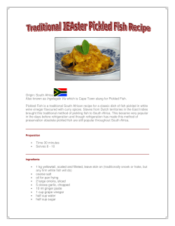
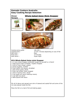

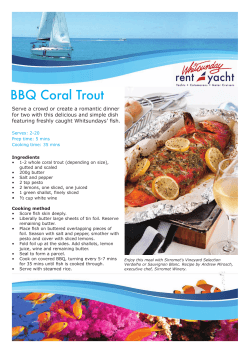
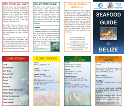


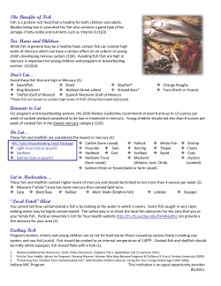
© Copyright 2026