1. science
2. physics

CERN-PH-TH-2014-191
INR-TH/2014-021
arXiv:1410.2408v1 [hep-th] 9 Oct 2014
Completing Lorentz violating massive gravity
at high energies∗
Diego Blas1, Sergey Sibiryakov1,2,3
1
2
CERN Theory division, CH-1211 Geneva 23, Switzerland
Institut de Th´eorie des Ph´enom`enes Physiques, EPFL, CH-1015 Lausanne, Switzerland
3
Institute for Nuclear Research of the Russian Academy of Sciences,
60th October Anniversary Prospect, 7a, 117312 Moscow, Russia
To Valery Rubakov,
Teacher and Colleague
Abstract
Theories with massive gravitons are interesting for a variety of physical applications,
ranging from cosmological phenomena to holographic modeling of condensed matter
systems. To date, they have been formulated as effective field theories with a cutoff
proportional to a positive power of the graviton mass mg and much smaller than that
of the massless theory (MP ≈ 1019 GeV in the case of general relativity). In this
paper we present an ultraviolet completion for massive gravity valid up to a high
energy scale independent of the graviton mass. This is achieved by the introduction of
vectors fields that develop condensates and spontaneously break the product of internal
and space-time symmetries to a diagonal subgroup. The perturbations of these fields
are massive and below their mass the theory reduces to a model of Lorentz violating
massive gravity. The latter theory possesses instantaneous modes whose consistent
quantization we discuss in detail. We briefly study some modifications to gravitational
phenomenology at low-energies. The homogeneous cosmological solutions are the same
as in the standard cosmology. The gravitational potential of point sources agrees with
the Newtonian one at distances small with respect to m−1
g . Interestingly, it becomes
repulsive at larger distances.
∗
Prepared for a special issue of JETP dedicated to the 60th birthday of Valery Rubakov.
1
Contents
1 Introduction
2
2 Lorentz violating massive gravity
5
3 Going beyond Λ2 : ingredients
3.1 The field φ0 . . . . . . . . . . . . . . . . . . . . . . . . . . . . . . . . . . . .
3.2 The fields φa and their coupling to Higgs vectors . . . . . . . . . . . . . . . .
8
8
10
4 Generation of VEVs in expanding backgrounds
13
5 Hierarchy of EFTs and the graviton mass
5.1 Phases with massive gravitons . . . . . . . . . . . . . . . . . . . . . . . . . .
5.2 Other phases? . . . . . . . . . . . . . . . . . . . . . . . . . . . . . . . . . . .
5.3 Quantum treatment of instantaneous modes . . . . . . . . . . . . . . . . . .
14
14
16
17
6 Modification of the Newton’s law
23
7 Summary and discussion
27
1
Introduction
Can gravity be mediated by a massive tensor field ? This straightforward question has
generated a lot of controversy since it was first formulated by Fierz and Pauli [1]. The
situation is remarkably different from the case of gauge interactions mediated by vector
fields, where the Higgs mechanism provides a clear-cut way to give mass to the vector
bosons within a weakly coupled theory. The differences fall into two categories. First, a
generic Lorentz invariant theory with massive spin-2 fields (gravitons) presents instabilities
in the sector of additional polarizations appearing in the massive, as opposed to massless,
case — the “Goldstone” sector. These instabilities arise around realistic backgrounds and
endanger the consistency of the theory even at low energies [2, 3]. It was first realized by
V. Rubakov [4] that these problems can be avoided by breaking the Lorentz invariance. This
approach has lead to the formulation of a class of Lorentz violating (LV) massive gravities
as consistent effective field theories (EFTs) [5] (see [6] for review). An alternative way to
improve the behavior of the Goldstone sector while preserving the Lorentz invariance has
been found in [7] and consists in a judicious choice of the couplings for the interactions of the
2
massive gravitons (see e.g. [8, 9]) for reviews). It has been argued [10, 11] that this tuning
might be stable under quantum corrections, but it is not clear at the moment if there is any
symmetry behind.
The second difference between massive spin-2 and spin-1 theories lies in their different
behavior at high energies. The interactions in the Goldstone sector of massive gravity become
strong and the perturbation theory breaks down at a certain cutoff scale1 Λlow depending on
the graviton mass mg . In the limit of vanishing mass this scale goes down to zero and, instead
of recovering the massless case, the theory ceases to exist. In fact, the same is also true for a
pure theory of massive vector fields with non-abelian interaction. However, in the latter case
the ultraviolet (UV) completion is known in the form of the Higgs mechanism which makes
the theory renormalizable by adding a handful of new degrees of freedom (Higgs bosons).
Importantly, in the resulting theory the massless limit is perfectly smooth and corresponds
to the restoration of the spontaneously broken gauge symmetry2 .
No such mechanism has been found so far for massive gravity3 . Of course, in this case one
cannot insist on an embedding into a fully UV complete theory — the massless theory being
non-renormalizable anyway with the cutoff at the Planck mass MP ≈ 1019 GeV (see, however,
Sec. 3.1). Still, it makes sense to search for a setup, whose cutoff would be independent of
the graviton mass and as close to the Planck scale as possible. To preserve the analogy
with the Higgs mechanism, the embedding theory must contain only a finite number of new
degrees of freedom compared to massive gravity itself4 , these degrees of freedom must be
weakly coupled and the limit mg → 0 must be regular. The goal of this work is to present a
setup fulfilling the above requirements.
The reasons for pursuing this endeavor are not merely academic. First, massive gravity
is a very natural candidate for an infrared (IR) modification of general relativity (GR) [16].
1
Throughout the paper we identify the cutoff with the strong coupling scale of the perturbation theory around the Minkowski background. In the setup of [7] the scale of strong coupling may be raised in
curved space-time due to the Vainshtein mechanism (see the discussion in [9]). However, the validity of the
corresponding backgrounds is under debate [12].
2
From a purist’s viewpoint, no symmetry is broken in the Higgs mechanism, gauge invariance being just
a redundancy in the description. However, we allow ourserves this abuse of terminology because of its clear
intuitive meaning.
3
Exceptions are theories in AdS where the mass of the graviton can appear due to non-trivial conditions
at the time-like boundary [13, 14, 15]. However, these constructions rely heavily on the peculiar properties
of the AdS geometry. In particular, the resulting graviton mass is always parametrically smaller than the
inverse AdS radius.
4
This excludes the known theories with massive spin-2 fields, such as Kaluza–Klein models or string
theory: both imply the presence of an infinite number of new degrees of freedom at the cutoff Λlow .
3
Such modifications are an interesting playground to look for alternatives to the cosmological
constant as the source of cosmic acceleration (see e.g. [17]). The acceleration may be
generated at the level of the background (new contribution to the Friedmann equation) or
of perturbations (weaker or repulsive gravitational potential at distances larger than m−1
g ).
It is fair to say that none of these possibilities have been satisfactory implemented so far in
concrete models. In any event, any candidate to explain cosmic acceleration should have a
completion at high energies, which is important for predictions related to the early universe
or very dense objects. This can also allow to understand the relevance of certain tunings of
the IR parameters. We will see how a concrete ultraviolet (UV) completion can have none
trivial consequences at very large distances.
Massive gravity has also been discussed in the context of the gauge/gravity correspondence [14, 15]. Various phases of massive gravity may be useful to describe different phenomenology at strong coupling. In particular, it was recently realized that LV massive gravity
is relevant for the description of systems with broken translational invariance [18, 19]. The
completion of the theory to smaller distances on the gravity side yields access to the operators
of higher dimensions in the strongly coupled field theory5 .
Finally, the theory of massive gravity is related to the spontaneous breaking of space-time
symmetries [20, 5]. This is an appropriate language to describe different states of matter
within the EFT framework [21, 22]. One can speculate that the Higgs mechanism for massive
gravity will be relevant to describe the phase transitions in such systems.
In this paper we will focus on the LV massive gravity of [4, 5]. Our main motivation
for this choice is the already mentioned validity of this theory as a low-energy EFT, whose
structure is protected by symmetries. Besides, the fundamental role of Lorentz invariance
in quantum gravity has been questioned recently [23]. It is interesting to explore if massive
gravity can be naturally embedded in this framework6 . We will assume that at the fundamental level the violation of Lorentz invariance is minimal and amounts to the existence of a
preferred foliation of space time [23, 25]. It is worth noting that the presence of superluminal
propagation [26, 27, 28] in the seemingly Lorentz invariant massive gravity of [7] makes a
Lorentz invariant Wilsonian UV completion of this theory problematic [29]. Thus, even in
this case the UV completion (if any) is likely to be Lorentz violating.
The paper is organized as follows. In Sec. 2 we briefly summarize the formalism of LV
massive gravity and define the phase that we will consider. In Sec. 3 we introduce the UV
completion that allows to push the cutoff of the theory to values close to MP . We analyze the
5
6
We thank Riccardo Rattazzi for the discussion of this point.
See [24] for an early attempt in this direction.
4
background solutions of the theory in Sec. 4 and show that the LV massive gravity of Sec. 2
appears in the IR limit. Section 5 is devoted to the analysis of the degrees of freedom in the
theory at different scales. We also discuss in some detail the quantization of instantaneous
modes present in the LV massive gravity and their relation to a certain type of non-locality
along the spatial directions. First results in phenomenology are presented in Sec. 6. We
conclude with the summary and discussion in Sec. 7.
2
Lorentz violating massive gravity
We will now briefly review the construction of LV massive gravity. We will formulate these
theories in a language closer to the symmetry breaking mechanism by introducing St¨
uckelberg
fields [20, 5]. This formulation is useful to understand many features of the theories, in
particular the strong coupling scale.
We focus on the setup where Lorentz invariance is broken down to the subgroup of spatial
rotations [4]. To describe this situation, let us consider four scalar St¨
uckelberg fields, φ0 , φa ,
a = 1, 2, 3, with internal SO(3) symmetry acting on the indices a, coupled to the metric in
a covariant way. Additional symmetries must be imposed on this sector to protect it from
pathologies [5]. We start by requiring invariance under the shifts7 of φ0 ,
φ0 7→ φ0 + const ,
(1a)
φa 7→ φa + f a (φ0 ) ,
(1b)
and the φ0 -dependent shifts of φa ,
where f a are arbitrary functions. We assume that in the stationary state the St¨
uckelberg
fields acquire coordinate-dependent vacuum expectation values (VEVs),
φ0 = µ20 t ,
φa = µ2 xa .
(2)
These VEVs break the product of 4-dimensional diffeomorphisms and the internal symmetries of St¨
uckelberg fields down to the diagonal subgroup consisting of the time shifts,
t 7→ t + const ,
(3a)
time-dependent shifts of the spatial coordinates,
xa 7→ xa + f a (t)
7
(3b)
We start from the simple φ0 -shifts to make contact with [5]. Later on we will promote them to a larger
symmetry, see Eq. (14).
5
and SO(3) spatial rotations. A simple Lagrangian that obeys the imposed symmetries and
admits the VEVs (2) has the form8 LS = LS1 + LS2 ,
X µν
1
κ0
0 2
4 2
0 2
4
(∂
φ
)
−
µ
−
(∂
φ
)
−
µ
P ∂µ φa ∂ν φa + 3µ4 ,
µ
µ
0
0
4
4
8µ0
4µ0
a
X
2
κ
1 X µν
2
P ∂µ φa ∂ν φb + µ4 δ ab + 4
P µν ∂µ φa ∂ν φa + 3µ4 ,
=− 4
8µ a,b
8µ
a
LS1 =
(4a)
LS2
(4b)
where κ0 , κ are dimensionless constants and
Pµν = gµν −
∂µ φ0 ∂ν φ0
,
g λρ ∂λ φ0 ∂ρ φ0
(5)
is the projector on the subspace orthogonal to the gradient of φ0 which ensures invariance
under (1b).
To understand the physical content of the theory, let us consider small fluctuations of the
metric and expand to the quadratic order in hµν ≡ gµν − ηµν . Using general covariance, we
can identify the coordinates with the St¨
uckelberg fields, as in (2). In other words, we work
0
a
in the gauge, where the fields φ , φ do not fluctuate. Then, the quadratic Lagrangian takes
the form,
µ4 κ0
µ4
µ4 κ 2
µ4
(2)
h00 haa − hab hab +
h ,
(6)
LS = 0 h200 −
8
4
8
8 aa
where the summation over repeated indices is understood. This is precisely a mass term for
the metric perturbation. In particular, the graviton (the helicity-2 component) acquires the
mass
µ2
mg =
,
(7)
MP
where MP is the Planck mass. Note that the term h0a h0a which is missing in (6) compared
to the most general expression [4] is forbidden by the residual symmetry (3b). The quadratic
Lagrangian of the form (6) appears also in bimetric theories [30, 31].
Let us return from the unitary gauge to the covariant Lagrangian (4) which is more
suitable to study the non-linear properties. Importantly, in the case when µ0 , µ are much
smaller than MP we can decouple the metric fluctuations and concentrate on the St¨
uckelberg
fields, as if they were living in flat space-time. We write
φ0 = µ20 t + ψ 0 ,
φa = µ2 xa + ψ a
8
(8)
This Lagrangian is not the most general one, but it is sufficient for our purposes, as it reproduces all
possible mass terms for the metric which are allowed by the symmetries (1).
6
and obtain
0
(ψ˙ 0 )2 κ0 µ2 ˙ 0
∂a ψ b ∂a ψ b (1 − κ)
∂ψ ∂ψ a
a
a 2
LS =
,
+ 2 ψ ∂a ψ −
−
(∂a ψ ) + Lint
,
2
µ0
4
4
µ20 µ2
(9)
where the last term stands for the derivative interactions of cubic and higher orders. By
power-counting, the strength of these interactions grows with the increase of energy or momentum and the theory breaks down at the scale
Λ = min{µ0 , µ} .
Comparing with (7) we conclude that the cutoff is bounded from above,
p
Λ < Λ2 ≡ mg MP .
(10)
(11)
Actually, this conclusion is not related to the specific form of the Lagrangian (4). As discussed
in [5], Λ2 provides an absolute upper bound on the cutoff in a general massive gravity theory
formulated in terms of the metric and St¨
uckelberg fields only9 . Thus the theory does not
admit a smooth limit mg → 0.
From the quadratic part of (9) we read off that a linear combination of ψ 0 and the
longitudinal part of ψ a has degenerate dispersion relation
ω2 = 0 .
(12)
This presents a potential danger, as in non-trivial backgrounds the r.h.s. of the dispersion
relation can become negative leading to an instability. In [5] it was suggested to lift the
degeneracy by adding to the Lagrangian quadratic terms with higher derivatives as in the
ghost condensate model [33]. In the next section we will take a different route and embed
the field φ0 into the khronometric model [25].
The rest of the modes in (9) — the transverse part of ψ a and the longitudinal component
of ψ a linearly independent from ψ 0 — obey the equations of the form,
k¯2 ψ = 0 ,
(13)
where k¯ is the absolute value of the three-momentum k¯i . Thus, for any non-zero spatial
momentum these modes must vanish implying that there are no propagating degrees of
freedom associated with ψ a . The symmetry (1b) ensures that this property is preserved
upon inclusion of higher-order operators [5] and in curved backgrounds [34]. Therefore the
theories based on the symmetries (1) present a class of well-defined EFTs10 .
9
The cutoff is even lower, Λ < Λ3 ≡ (m2g MP )1/3 , if one restricts to the Lorentz invariant theories [20, 32].
A subtle issue of the proper treatment of the non-propagating modes at the quantum level will be
discussed in Sec. 5.3.
10
7
3
3.1
Going beyond Λ2: ingredients
The field φ0
There are two natural ways to deal with the field φ0 to complete the previous actions to
energies higher than (10). First, as we mentioned above, the degeneracy of the dispersion
relation (12) can be lifted by adding higher derivative terms as in the ghost condensate [33].
This theory is still an effective theory with a cutoff of order µ0 , but since this is independent
of the mass of the graviton, this scale can be quite high. Phenomenological bounds set the
constrain µ0 . 10 MeV. It was argued in [35] that these bounds can be relaxed by the
non-linear dynamics which may push the upper limit on µ0 to 100 GeV. This still remains
much below the Planck scale. The way to raise the cutoff of the theory to (almost) Planckian
was proposed in [36]. It uses the embedding of the ghost condensate into the khronometric
model [25] and requires the introduction of a new degree of freedom — khronon — at a scale
below µ0 . One could use this strategy here.
However, it is more economical to use the second option and identify the St¨
uckelberg field
φ0 directly with the khronon, thus keeping only a single degree of freedom in this sector. In
this case the symmetry (1a) is extended to the full reparameterization invariance,
φ0 7→ f 0 (φ0 ) ,
(14)
for an arbitrary monotonic function f 0 . This larger symmetry forbids the terms present in
(4a). Instead, the Lagrangian must be constructed using the unit vector
uµ ≡ p
∂µ φ0
g λρ ∂λ φ0 ∂ρ φ0
(15)
invariant under the symmetry (14). The most general Lagrangian with the lowest number
of derivatives, and thus dominant at low energies, reads [25],
Lkh = −
MP2
R + β∇µ uν ∇ν uµ + λ(∇µ uµ )2 + αuµ uν ∇µ uρ∇ν uρ ,
2
(16)
where we have also included the standard GR action; α, β, λ are dimensionless coupling
constants. This can be combined with (4b) to give an action of LV massive gravity. Note
that in the unitary gauge11 (2) the Lagrangian (16) gives rise only to terms with derivatives
11
Because of the invariance (14) the choice of the constant µ20 in the first formula of (2) is now arbitrary
and unrelated to the parameters of the theory.
8
of the metric perturbations and thus does not contribute to the mass term for hµν . The
latter reduces to
µ4
µ4 κ 2
Lmass = − hab hab +
h .
(17)
8
8 aa
This can be understood as the consequence of the time-reparameterization invariance
t 7→ f 0 (t) ,
(18)
which, being now a residual symmetry in the unitary gauge, forbids any contributions containing h00 without derivatives. This version of massive gravity was considered in [37].
The Lagrangian (16) contains higher derivatives of the field φ0 and one may be worried
that this can lead to pathologies (ghosts or gradient instabilities). In fact, this does not
happen, as the extra derivatives act in the spatial directions. This property becomes explicit
in the gauge where the time coordinate is identified with φ0 as in the first equation of (2).
Note, that this identification still leaves the free choice of the spatial coordinates, so it should
not be confused with the unitary gauge where all coordinates are fixed. We will call this
partial gauge fixing ADM gauge. The action of the khronometric model takes the form,
2 Z
MP2
∂i N
3 √
ij
2
(3)
dt d x γN (1 − β)Kij K − (1 + λ)K + R + α
,
(19)
Skh =
2
N
where we used the Arnowitt–Deser–Misner (ADM) decomposition for the metric,
ds2 = dt2 − γij (dxi + N i dt)(dxj + N j dt) ,
(20)
the extrinsic curvature of the constant-time slices
Kij =
1
(γ˙ ij − ∇i Nj − ∇j Ni ) ,
2N
K = γ ij Kij ,
(21)
and denoted (3) R the three-dimensional curvature constructed from the metric γij . Apart
from the symmetry (18), this action is invariant under time-dependent spatial diffeomorphisms
xi 7→ x˜i (x, t) .
(22)
We will refer to the group consisting of the transformations (18) and (22) as foliationpreserving diffeomorphisms (FDiff). Clearly, the action (19) leads to equations of motion
which are second order in time derivatives. We will work in the ADM gauge from now on.
The choice α = β = λ = 0 corresponds to GR and the restoration of the full diffeomorphisms-invariance. However, the limit α, β, λ → 0 is not smooth. At any non-zero values of
α, β, λ the theory propagates in addition to the helicity-2 gravitons a single helicity-0 mode
9
(khronon). The latter has linear dispersion relation; in the case α, β, λ ≪ 1 (which is the
relevant one for phenomenology) it reads12 [25],
ω2 =
β+λ 2
k .
α
(23)
Due to the non-linear interactions of the khronon present in (19) the model has a cutoff
√ p √
Λkh ∼ MP min{ α, β, λ} .
(24)
Phenomenological considerations put upper bounds on α, β, λ [25, 38, 39] and hence constrain the cutoff to be somewhat smaller than the Planck scale,
Λkh . 1015 GeV .
(25)
Still, this is well above virtually any scale that can appear in the astrophysical or cosmological context13 . Furthermore, it is known how to complete the action (19) beyond Λkh
by embedding it into the Hoˇrava gravity [23, 40]. The latter presents a power-counting
renormalizable theory. However, due to the technical complexity, the question about its
renormalizability in the strict sense and UV behavior still remains open (see Refs. [41, 42]
addressing this issue in restricted settings). In these circumstances a cautious reader may
prefer to take modest attitude and view the khronometric model as an EFT with the cutoff
(24), which is sufficient for the purposes of this work.
Finally, let us mention the following peculiarity of the action (19). As described in [25],
it leads to a certain type of instantaneous interactions mediated by a non-propagating mode.
The latter is similar to the non-propagating modes of massive gravity discussed in Sec. 2.
We will study the instantaneous modes in more detail in Sec. 5.3.
3.2
The fields φa and their coupling to Higgs vectors
Next we consider the triplet of St¨
uckelberg fields invariant under
φa 7→ φa + f a (t) ,
(26)
which is nothing but the symmetry (1b) in the ADM gauge. We want a Lagrangian that
admits the coordinate-dependent VEVs (2), but at the same time is UV complete past
12
This relation gets modified — in particular, the khronon acquires a mass gap — when the action (19) is
coupled to the other sectors needed to reproduce the massive gravity, see Sec. 6 below.
13
In the applications unrelated to astrophysics, such as non-relativistic holography or description of solids,
the parameters α, β, λ are a priori constrained only by the stability requirements, that are quite mild, and
the scale Λkh can be as high as MP .
10
the scale µ. This precludes from introducing any self-interaction of the St¨
uckelberg fields
involving the scale µ. Then the simplest option is to choose the Lagrangian to be quadratic
in φa . To respect the symmetry (26), it must depend only on the spatial derivatives of these
fields,
Z
1 ij a
3 √
a
Sφ = dt d x γN − γ ∂i φ ∂j φ .
(27)
2
This does not introduce any new strong coupling scale. However, without any further interactions this Lagrangian is not enough to provide non-zero graviton mass. Though the
configuration φa = Φxa is a solution of the equations following from (27) for any constant Φ,
it introduces non-vanishing energy density and pressure which make the universe expand14 .
As will become clear in the Sec. 4, in this case the generated mass will decrease with time
and will asymptotically vanish. Time varying masses can be interesting (see e.g. [34]) but
are not the aim of this paper. To give constant graviton mass, the VEVs must grow proportionally to the scale factor, φa ∝ a(t)xa which is not a solution of the field equations implied
by (19) and (27). We have to add more ingredients.
Consider a triplet of vector fields with purely spatial components Vai . These transform
as vectors under the diffeomorphisms preserving the foliation structure of the ADM gauge,
which act on the i-index. Besides, they form the fundamental representation of a global
internal SO(3) acting on the index a. We do not assume any gauge invariance associated to
these vectors. To avoid strong coupling, we focus on Lagrangians which are renormalizable in
flat space-time. By the standard power-counting, they can contain the derivatives of Vai only
quadratically and up to quartic terms in the potential. The generic Lagrangian satisfying
these properties and invariant under FDiff × SO(3) reads
Z
c21
c22
1 ˙i
3 √
j
i
j
i 2
j 2
SV = dtd x γN
(
V
−
N
∇
V
+
V
∇
N
)
−
(∇
V
)
−
(∇i Vai )2
j
j
i
a
a
a
a
2
2N
2
2
(28)
κ2 i j
κ1 i j
2
2
2 2
− (Va Vb γij − MV δab ) − (Va Va γij − 3MV ) ,
4
4
where c1 , c2 , κ1 , κ2 are dimensionless couplings and we have chosen the overall constant
in the potential to have vanishing vacuum energy (we will shortly introduce a cosmological
constant term in a different part of the action). For clarity, we have omitted non-minimal
interactions with the metric, such as (3) Rij Vai Vaj , (3) RVai Vaj γij , which vanish in Minkowski
space-time. These terms would make the analysis more cumbersome without changing it
qualitatively.
14
These density and pressure cannot be canceled by any bare cosmological constant.
11
When MV2 > 0 the vectors develop VEVs,
Vai = MV δai ,
(29)
which break the product SO(3)×SO(3) of spatial and internal rotations down to the diagonal
√
subgroup, cf. [43, 44, 45, 46]. Below the scale ∼ κMV the dynamics is described by the
σ-model corresponding to this pattern of symmetry breaking with the coset space defined
by
Vai Vbj γij = MV2 δab .
(30)
As the vector VEVs introduce an additional source of Lorentz symmetry breaking, it is
natural to expect that the phenomenological constraint on the scale MV will be similar to
that of Λkh , Eq. (25). Notice, however, that MV is not related to the cutoff and can be much
lower than Λkh without jeopardizing the validity of the theory.
Finally, we complete our Lagrangian with a term mixing the vectors and the St¨
uckelberg
fields,
Z
√ SV φ = dt d3 x γN mA Vai ∂i φa − V0 .
(31)
This mixing operator has dimension 3 and thus is just a relevant deformation of the previous
action. It does not affect the UV properties of the theory, in particular, it does not introduce
any new UV cutoff, and the parameter mA can be arbitrarily small without encountering
any singularity. We are going to see that in IR this coupling leads to the generation of the
VEVs (2) with µ2 = mA MV and the graviton mass (7). The last term in (31) represents a
cosmological constant and can be tuned to cancel the negative vacuum energy that would
be generated otherwise (see below). Note that it is technically natural to take the parameter
mA to be much smaller than the other scales of the theory as it is protected from large
quantum corrections by the discrete symmetry15 φa 7→ −φa . In what follows we will assume
the hierarchy of scales,
MP & Λkh & MV ≫ mA .
(32)
It is worth stressing that this hierarchy is not required by the internal consistency of the
theory. For example, one could consider instead mA ∼ MV . However, assuming (32) makes
the physical picture particularly transparent.
15
A similar argument is used to protect the small coupling between a time-like vector field and an ordinary
massless scalar in the technically natural dark energy model of [47].
12
4
Generation of VEVs in expanding backgrounds
Let us now show that the construction of the previous section gives rise to the VEVs for the
fields φa of the desired form. We assume a homogeneous and isotropic Ansatz with spatially
flat metric allowing for a general cosmological evolution,
N(t) ,
γij = a2 (t)δij ,
Vai =
MV i
δ ,
a(t) a
φa = Φ(t)xa .
(33)
Substituting this Ansatz into the equations of motion obtained from putting together the
actions (19), (27), (28) and (31) we obtain,16
3Φ2
3µ2 Φ
+
− V0 = ρmat ,
2a(t)2
a(t)
2µ2 Φ
Φ2
+
− V0 = −pmat ,
2Mc2 H˙ + 3Mc2 H 2 −
2a(t)2
a(t)
3Mc2 H 2 −
(34a)
(34b)
where
and
Mc2
≡
MP2
µ2 = mA MV
(35)
M2
β + 3λ
− V,
1+
2
2
(36)
is the “cosmological Planck mass”. In Eqs. (34) we fixed the gauge N = 1 and assumed that
the universe is filled with matter with energy density ρmat and pressure pmat . Taking the
derivative of (34a) and using the energy conservation in the matter sector,
ρ˙ mat + 3H(ρmat + pmat ) = 0 ,
(37)
we obtain the following equation for Φ,
˙
Φ(Φ
− µ2 a(t)) = 0 .
(38)
This has two branches of solutions. On the branch Φ = const the VEVs of the St¨
uckelberg
fields actually disappear with time. Indeed, the invariant quantity γ ij ∂i φa ∂j φa = 3Φ2 /a(t)2
decreases as the universe expands. Besides, we will see shortly that this branch is unstable
whenever µ 6= 0. The other branch is
Φ = µ2 a(t) .
16
(39)
The simplest way to derive these equations is to substitute the Ansatz (33) into the action and perform
variation with respect to the free functions N (t) and a(t) afterwards. Note, however, that it would be
incorrect to vary this action with respect to Φ as the corresponding variation δφa = δΦxa would not be
bounded at spatial infinity.
13
It corresponds to constant strength of the St¨
uckelberg fields’ gradients and is stable. In this
latter case the cosmological equations (34) reduce to the form,
3Mc2 H 2 = ρmat + V0 −
3µ4
,
2
(40a)
3µ4
2Mc2 H˙ + 3Mc2 H 2 = −pmat + V0 −
.
(40b)
2
We see that role of µ in this phase is to renormalize the cosmological constant to a smaller
value. In what follows we will assume that this contribution is canceled by the bare cosmological constant,
3µ4
,
(41)
V0 =
2
so that the Minkowski space-time is a solution in the absence of matter. This is just the
usual fine-tuning of the cosmological constant.
5
5.1
Hierarchy of EFTs and the graviton mass
Phases with massive gravitons
To understand the effect of the mixing term (31) on the spectrum of the theory let us study
small perturbations. As before, we work in the ADM gauge and first focus on the phase
with a vacuum from the branch of solutions (39). To simplify the analysis, we freeze out the
perturbations in the khronometric sector by sending MP and Λkh to infinity while keeping
MV and mA finite. For the perturbations of the vectors and the St¨
uckelberg fields we write,
Vai = MV δai + vai , φa = µ2 xa + ψ a .
(42)
√
If we are interested in energies below κMV we can adopt the σ-model description. Inserting
(42) in the constraint equation (30) yields,
vai
=
Aia
Aji Aja
+ O(A3 ) ,
−
2MV
(43)
where Aia is an antisymmetric matrix, Aia + Aai = 0. Substituting this into the Lagrangian
we obtain,
(∂i ψ a )2 m2A j j
−
A A + mA Aia ∂i ψ a .
(44)
Lφ + LV φ = −
2
2 a a
The second term gives mass of order mA to the antisymmetric perturbations Aia . Below this
scale the perturbations of the vectors can be integrated out completely. From (44) we find
Aia =
1
(∂i ψ a − ∂a ψ i ) ,
2mA
14
(45)
which substituted back into (44) gives (up to a total derivative)
Lφ + LV φ = −
∂i ψ a ∂i ψ a (∂a ψ a )2
−
.
4
4
(46)
This coincides with the third and fourth terms (with κ = 0) of the quadratic St¨
uckelberg
a
Lagrangian (9) arising in massive gravity. The “massless” fields ψ can be interpreted as
the Goldstone bosons for the broken symmetries FDiff × SO(3) → SO(3)diag . Recall that
since we are dealing with LV theories, the counting and properties of such fields are different
from the Lorentz invariant case, see e.g. [48, 49, 50]. Given the previous results, we expect
that the graviton in this model will acquire the mass (7). For the case MP ≫ MV the vector
and graviton masses are well separated and at energies mA ≫ E ≫ mg the dynamics is
well described by the EFT for the St¨
uckelberg fields. The hierarchy of various scales in the
theory and the corresponding EFT descriptions are summarized in Fig. 1.
Alternatively, we can work in the unitary gauge and fix ψ a = 0 at the expense of allowing
for the fluctuations of the metric
N =1+n ,
Ni ,
γij = δij + hij .
The relevant part of the Lagrangian takes the form,
Vaa
3
γ aa
4
.
+
−
Lφ + LV φ = µ −
2
MV
2
(47)
(48)
The solution of the constraint (30) now reads,
vai
=
Aia
MV
Aji Aja Aji hja Aja hji 3MV
−
−
hai −
−
+
hji hja + O(A3 , h3 ) .
2
2MV
4
4
8
(49)
Substituting this formula and the expression
γ ij = δij − hij + hik hkj + O(h3 )
(50)
into (48) we obtain at the quadratic level,
Lφ + LV φ = −
m2A i i µ4
A A − hia hia .
2 a a
8
(51)
The first term again gives mass to the antisymmetric perturbations, while the second explicitly provides the mass term for helicity-2 graviton. As we are going to see in Sec. 6, it also
gives mass to the khronon (see Eq. (83)). Note that we obtain only one of the two structures
for the metric mass term allowed by the symmetries, cf. (17). This a consequence of the
15
Figure 1: Relevant energy scales in the theory and the number of propagating degrees of
freedom in each sector at different scales. Rectangles represent the energy scales at which a
sector gets UV completed (we do not make any assumptions about the UV completion of the
khronon and spin-2 sectors, but Hoˇrava gravity [23] would be a natural option). Rhomboids
mark the scales below which a sector loses all its propagating degrees of freedom. Note that
nothing happens at the scale µ ≡ Λ2 which set the cutoff in the original EFT formulation of
massive gravity.
assumption MV ≫ mA which implies that the symmetric part of the vector fluctuations is
√
much heavier (with the mass of order κMV ) than the antisymmetric part. This renders
the parameter κ in (17) suppressed by the ratio m2A /κMV2 which we neglected in the above
analysis. Were we to make a different assumption MV ∼ mA , we would obtain both terms
of (17) with comparable coefficients. Finally, if instead of the khronometric setting one used
the ghost condensate for the φ0 -sector, which in the ADM gauge amounts to promoting all
couplings in the action to functions of the lapse N [25], one would be able to reproduce also
the other terms in the general Lagrangian (6) of the massive gravity discussed in Sec. 2.
5.2
Other phases?
In the previous section we focused on the branch (39) of the background solutions. However,
as noticed before, the equation (38) also admits a second branch
Φ˙ = 0 .
(52)
On this branch the effect of the St¨
uckelberg gradients (if non-zero initially) decays with time
in an expanding universe. For completeness we now analyze the small perturbations around
16
this branch. We write,
φa = Φxa + ψ a ,
(53)
with Φ = const and take the Friedmann–Robertson–Walker (FRW) form for the metric. We
again work in the decoupling limit MP , Λkh → ∞, so that the metric fluctuations are frozen.
√
Below the scale κMV the fluctuations of the vectors are restricted to the antisymmetric
part Aia . Expanding the relevant part of the action to quadratic order we obtain,
SV + Sφ + SV φ =
3
Z
a2 m Φ
a ˙i 2 a 2
A
3
j 2
2
i 2
a 2
i 2
2
i
a
dt d x
c (∂i Aa ) + c2 (∂i Aa ) + (∂i ψ ) −
(A ) −
(Aa ) + a mA Aa ∂i ψ .
2 a
2 1
2MV
(54)
Restricting to the modes with frequencies much higher than the Hubble rate, we can neglect
the terms with derivatives of the scale factor in the equations of motion. This yields,
c2
c2
mA Φ i mA
− A¨ia + 12 ∂j2 Aia + 22 ∂j ∂[i Aja] −
A +
∂[i ψ a] = 0 ,
a
a
MV a a
a
∂i2 ψ a − amA ∂i Aia = 0 ,
(55a)
(55b)
where the square brackets stand for the antisymmetrization of indices. Let us perform the
Fourier transform and concentrate on the transverse modes
a
ψ =
e(α)
a ψ(α)
,
Aia
(α)
(α)
k¯i ea − k¯a ei
A(α) ,
=
k¯
(56)
(α)
where ei , α = 1, 2, are unit polarization vectors orthogonal to the 3-momentum k¯i . Substituting this into Eqs. (55) and eliminating ψ(α) we obtain,
c22 k¯2
mA Φ µ2
2
2
ω − c1 +
A(α) = 0 ,
(57)
−
−
2 a2 MV a
2
where we used µ2 defined in (35). We see that whenever Φ < µ2 a/2 the mode is tachyonic. In
particular, the trivial configuration of the St¨
uckelberg fields φa = 0 is unstable. Furthermore,
in an expanding universe µ2 a/2 will exceed any constant value of Φ and the instability will
set in at late times. Thus we conclude that in an expanding universe this branch is unstable
and we do not consider it any more in this paper.
5.3
Quantum treatment of instantaneous modes
We have argued above that the constructed model is a valid quantum theory up to the scale
(24). We have based this claim on the scaling argument borrowed from relativistic theories,
17
so it is worth taking a closer look at it to check if it is not spoiled by Lorentz violation.
To get a flavor of the potential problems consider the instantaneous modes φa . Let us first
switch off their mixing with the vectors by setting mA = 0 and perform their perturbative
quantization using the path integral formalism. From (27) one reads off the propagator,
φa
p
φb = −
i ab
δ ,
p¯2
(58)
where we denoted by the bar the spatial part of a four-vector pµ = (p0 , p¯i ). This propagator
does not depend on the frequency p0 . The fields φa couple to the metric and contribute into
the effective action for the perturbations hij . For example, the one-loop contribution into
the quadratic part is
p+q
ij
kl
h
h
1
= hij (p)hkl (−p)
4
Z
dq0
2π
Z
d3 q¯ q¯i q¯k (¯
q + p¯)j (¯
q + p¯)l
.
(2π)3
q¯2 (¯
q + p¯)2
(59)
q
This expression contains two types of divergences. The integral over the spatial momentum
can be regulated by subtracting a finite number of local counterterms. However, the whole
contribution will still be infinite because of the overall divergent integral over q0 . Note that
this divergence has non-polynomial dependence on the external spatial momentum p¯i and
therefore is non-local in space. On the other hand, it does not depend on p0 and hence is local
in time. Thus it can be regulated by introducing a spatially non-local counterterm in the
bare action. Though unusual, such counterterms do not spoil the validity of the theory. In
particular, the diagram (59) does not contain any imaginary part and thus the corresponding
counterterm does not violate unitarity.
One may object that allowing for non-locality, even restricted to only spatial dimensions,
introduces an infinite freedom in the choice of the bare action. However, we now argue that
there is a natural choice of counterterms for the diagrams where, like in (59), a divergent
integral over the loop frequency completely factors out of a frequency-independent part.
This consists in canceling these diagrams altogether. In the present case this would mean
that all loop diagrams containing the instantaneous fields φa must be put to zero. Two
arguments support this prescription. First, the integrals over frequency diverge linearly and
thus vanish identically in dimensional regularization. Second, we can appeal to the canonical
quantization. In this formalism, the fields φa are subject to second-class constraints which
force them to vanish. Indeed, as the action does not depend on the time-derivative of these
18
fields, the canonical momenta conjugate to them vanish trivially, while the fields themselves
obey the equation,
∇i (N∇i φa ) = 0 .
(60)
Supplemented by the vanishing boundary conditions at spatial infinity it forces17 φa = 0.
In the canonical approach such constrained degrees of freedom must be eliminated from the
start, even prior to quantization, implying that they completely drop off from the quantum
theory18 .
There is a way to implement the above prescription within the path integral approach
without introducing non-local counterterms from the start. One notices that the overall
result of integration over φa is a factor
det(iγ ij ∂i ∂j )
−3/2
(61)
in the partition function. This can be canceled by adding to the system three real bosonic
fields φ˜a and three complex fermionic fields η a with the action,
Z
1 ij ˜a ˜a
ij
a
a
3 √
(62)
Sφη
dt d x γN − γ ∂i φ ∂j φ − γ ∂i η ∂j η¯ .
˜ =
2
Integrating out these “remover” fields multiplies the partition function by,
3
3/2
det(iγ ij ∂i ∂j )
ij
,
3/2 = det(iγ ∂i ∂j )
det(iγ ij ∂i ∂j )
(63)
which precisely compensates (61). The expression (63) corresponds to the spatially non-local
counterterms discussed above.
Turning on mA makes the situation less trivial. However, given that the mixing (31) is
a relevant deformation it clearly cannot spoil the UV consistency of the theory. A comprehensive analysis of the quantum properties of the theory introduced in Sec. 3 is beyond the
scope of this paper. Instead, we illustrate the expected behavior in a toy model containing
17
Multiplying (60) by φa and integrating over the three-dimensional space we obtain,
Z
Z
0 = d3 x φa ∇i (N ∇i φa ) = − d3 x N ∇i φa ∇i φa .
As the lapse function is non-zero everywhere, one concludes that ∇i φa = 0 and hence φa vanishes due to
the boundary conditions.
18
There is no modification of the canonical structure for the remaining fields as in the case at hand Dirac
and Poisson brackets are identical.
19
a scalar and a vector without any VEVs in an external non-dynamical metric (we assume
Ni = 0),
S=
Z
˙i˙j
γij V V
γjk ∇i V j ∇i V k 1 ij
MV2
√
i
i j
dtd x γN
−
− γ ∂i φ∂j φ+mA V ∂i φ−
γij V V . (64)
2N 2
2
2
2
3
For simplicity, we have retained only one of the gradient terms for the vector putting the
coefficient in front of it to c21 = 1. As before, there are two ways to proceed. In the canonical
approach we have to solve for the field φ before quantization,
φ=
mA (∇i V i + ai V i )
,
γ kl ∇k ∇l + al ∇l
(65)
ai ≡ N −1 ∂i N .
(66)
where
Substituting this into (64) we obtain a non-local action which depends only on V i ,
S=
Z
˙i˙j
γjk ∇i V j ∇i V k MV2 γij V i V j
√
γij V V
−
−
dt d x γN
2N 2
2
2
m2A
j
j
i
i
(∇j V + aj V ) .
− (∇i V + ai V )
2(γ kl ∇k ∇l + ak ∇k )
3
(67)
The Dirac bracket remains identical to the canonical commutator. One observes that the
limit mA → 0 is smooth and corresponds to restoration of locality. As non-locality is purely
spatial, it does not, in principle, present an obstruction to canonical quantization.
However, in practice it is very inconvenient to work with the non-local action (67). It is
more efficient to use the path integral approach and retain φ as a quantum field. Assuming
that the metric is close to flat, we obtain from (64) the propagators for φ and V i ,
φ
φ
Vi
p
p
p
i
im2A
+
,
p¯2 p¯2 (p20 − p¯2 − MV2 + m2A )
−mA p¯i
,
Vi = 2 2
p¯ (p0 − p¯2 − MV2 + m2A )
p
¯
p
¯
i
p¯i p¯j
i
i
j
+ 2 2
.
V j = δij − 2
2
2
2
2
p¯
p¯0 − p¯ − MV
p¯ p0 − p¯ − MV2 + m2A
φ =−
(68a)
(68b)
(68c)
To avoid cluttered formulas, we will set MV = mA in what follows. This does not affect
the UV properties of the theory. Consider again the diagram (59). Now it contains three
contributions. The first one comes from the product of the first terms in the propagator
˜ η with the
(68a) and, as before, is eliminated by adding to the path integral the fields φ,
20
action (62). Besides, there are contributions coming from the cross-product of the two terms
in (68a),
Z
m2A ij
dq0 d3 q¯ q¯i q¯k (q + p¯)j (¯
q + p¯)l
kl
−
h (p)h (−p)
,
(69)
2
4
2
2
2
(2π) q¯ (q0 − q¯ )(¯
q + p¯)2
as well as from the square of the second term,
Z
dq0 d3 q¯
q¯i q¯k (¯
q + p¯)j (¯
q + p¯)l
m4A ij
kl
h (p)h (−p)
.
2
4
2
2
2
4
(2π) q¯ (q0 − q¯ )(¯
q + p¯) ((q0 + p0 )2 − (¯
q + p¯)2 )
(70)
The divergences in these expressions can be removed by genuinely local counterterms. Consider, for example, Eq. (69). Introducing Feynman parameters we obtain,
Z
Z
Z
Z 1
dq0 d3 q¯ q¯i q¯k (¯
dq0′ d3 q¯
q + p¯)j (¯
q + p¯)l
q¯i q¯k (¯
q + p¯)j (¯
q + p¯)l
dx1 1−x1
,
dx
=
2
√
2
2
2
4
2
2
2
4
(2π) q¯ (q0 − q¯ )(q + p)
x1 0
(2π) (q0′ − q¯2 − 2¯
q p¯x2 − p¯2 x2 )3
0
(71)
where in the last integral we rescaled the loop frequency. The integral over the fourmomentum on the r.h.s. has the standard form and its divergent part is a polynomial
in momenta p¯. It is straightforward to check that the integration over Feynman parameters
does not contain any additional divergences. Thus, we conclude that the overall divergence
of (71) is local both in time and space. Similar reasoning applies to (70).
One may worry that a divergence in the Feynman parameters can appear in the diagrams
that contain the loop frequency in the numerator of the integrand, because then more powers
of the Feynman parameters descend into the denominator. Let us show that this does not
happen. Consider the diagram arising from the interactions given by the first and the third
terms in (64),
p+q
Z
2
m
dq0 d3 q¯
q0 (q0 + p0 )¯
qi q¯k (¯
q + p¯)j (¯
q + p¯)l
A
kl
kl =
h
(p)h
(−p)
.
ij
h
2
2
(2π)4 q¯2 (q0 − q¯2 )(¯
q + p¯)2 ((q0 +p0 )2 −(¯
q + p¯)2 )
hij
q
(72)
Passing to the Feynman parameterization we obtain,
Z
dq0 d3 q¯
q0 (q0 + p0 )¯
qi q¯k (¯
q + p¯)j (¯
q + p¯)l
2
4
2
2
2
2
(2π) q¯ (q0 − q¯ )(¯
q + p¯) ((q0 + p0 ) − (¯
q + p¯)2 )
Z 1
Z 1−x1
Z 1−x1 −x2
=6
dx1
dx2
dx3
(73)
0
0
0
Z
q0 (q0 + p0 )¯
qi q¯k (¯
q + p¯)j (¯
q + p¯)l
dq0 d3 q¯
×
4 .
4
2
2
(2π) (x1 + x2 )q0 + 2q0 p0 x2 + p0 x2 − q¯2 − 2¯
qp¯(x2 + x3 ) − p¯2 (x2 + x3 )
21
Figure 2: Generic diagram with instantaneous modes and gravitons propagating in the loops.
Summing it with the diagrams of the same topology where the different subsets of the φ-loops
are replaced by those of φ˜ and η will remove all non-local divergences.
√
Upon rescaling of the loop frequency, q0 7→ q0′ = q0 / x1 + x2 , the most singular contribution
in the integral over Feynman parameters is proportional to (x1 + x2 )−3/2 which is again
integrable. At the heuristic level this can be understood as follows. The divergences in
the integrals over Feynman parameters are usually associated to the infrared (or collinear)
divergences, which are absent in our case because the original expressions (69) and (72) are
IR safe.
By extending the above reasoning to other diagrams in the model (64) the reader will
easily convince herself that the only class of divergences that require (spatially) non-local
counterterms are those where all propagators in a given loop are equated to the first term
in (68a). These divergences are independent of mA and are exactly canceled by the remover
˜ η with the action (62). Furthermore, this cancellation persists upon making the
fields φ,
metric hij dynamical and allowing it to propagate in the loops. Thus, it is natural to
conjecture that no matter how complicated a diagram is (see an example in Fig. 2), it will
require only local counterterms after addition of similar diagrams with the fields φ˜ and η.
So far we have discussed only the instantaneous modes associated with the St¨
uckelberg
a
fields φ of massive gravity. The dynamics of these fields is relatively simple: they enter
in the UV action (27), (31) quadratically and do not contain any propagating degrees of
freedom. This allowed us to eliminate all unusual non-local divergences appearing due to
these fields by adding the “remover” sector φ˜a , η a with the simple action (62). However, as
pointed out in [25], another source of instantaneous interactions is the khronon field φ0 . Here
22
the situation appears more complicated: the khronon describes, besides the instantaneous
mode, a genuine propagating degree of freedom and, furthermore, enters into the action nonlinearly. This produces difficulties with the quantization which are intrinsic of Hoˇrava (or
khronometric) proposal. We plan to address them elsewhere. For now, we just point out that
the above discussion suggests that a consistent quantization of the theory exists. Indeed, in
the decoupling limit the propagator of the khronon has the form similar to the second term
in (68a) [25]. We have seen that the divergences associated with such propagators can be
removed by local counterterms.
6
Modification of the Newton’s law
Having addressed the theoretical consistency of the model, we now study its immediate phenomenological consequences. Let us consider the gravitational field of a point mass M⊙ at a
fixed position xi = 0. We will focus on the weak field (linear) regime and assume the minimal
coupling of the metric to the matter sector; the latter is justified by the phenomenological
constraints on deviations from the Lorentz invariance [51]. There are two important changes
with respect to the massive gravity phase (3) described in [5, 52]. First, at any energy the
role of the St¨
uckelberg field φ0 is played by the khronon. Second, the theory is defined also
above the energy Λ2 , which can have experimental consequences at short distances relevant
e.g. in the early universe or in very dense stars. We will only consider the large distance
modification in this section.
We work in the unitary gauge19 , and restrict the vector fields to the coset space (30).
We consider the scalar part of the perturbations. The expansion around the Minkowski
background to linear order reads,
N =1+ϕ,
(74a)
Ni = ∂i B ,
(74b)
∂i ∂j
∂i ∂j
γij = δij − 2 δij −
Ψ−2
E,
∆
∆
∂i ∂a
∂i ∂a
i
i
Ψ + MV
E,
Va = MV δa + ǫiaj ∂j C + MV δia −
∆
∆
(74c)
(74d)
where we have used the linear part of Eq. (49). Using the expression (51) and expanding
19
Recall that it is consistent to first fix the unitary gauge and take the variation of the action afterwards [53].
23
the khronometric and vector Lagrangians (19) and (28) to quadratic order one obtains20 ,
MP2
(2)
˙ 2 + 4ΨE
¨ + 4Ψ∆B)
˙ − (λ + β)(2Ψ
˙ + E˙ + ∆B)2
Lscal =
(1 − β)(−2Ψ
2
MV2 ˙ 2
2
2
2
2
2
˙
(75)
2Ψ + (E + ∆B) − 4(c1 + c2 )(∂i Ψ)
− 2Ψ∆Ψ + 4ϕ∆Ψ + α(∂i ϕ) +
2
4
˙ 2 − c2 (∂i ∂k C)2 − µ4 Ψ2 − µ E 2 − m2 (∂i C)2 − ϕM⊙ δ(x) .
+ (∂i C)
1
A
2
We see that the pseudoscalar mode C completely decouples and has the dispersion relation
ω 2 = c21 k¯ 2 + m2A .
(76)
For the other components we obtain the set of equations,
2MP2 ∆Ψ − αMP2 ∆ϕ − M⊙ δ(x) = 0 ,
˙ + M 2 (λ + β) − M 2 (E˙ + ∆B) = 0 ,
2MP2 (1 + λ)Ψ
P
V
2
¨ + MP2 (1 + λ)(E
¨ + ∆B)
˙
MP (1 + β + 2λ) − MV2 Ψ
2
− MP − 2MV2 (c21 + c22 ) ∆Ψ − µ4 Ψ + MP2 ∆ϕ = 0 ,
¨ + M 2 (λ + β) − M 2 (E¨ + ∆B)
˙ − µ4 E = 0 .
2M 2 (1 + λ)Ψ
P
P
V
(77a)
(77b)
(77c)
(77d)
Combining the second and fourth equations we find
E=0,
∆B = −
2MP2 (1 + λ)
˙ .
Ψ
MP2 (λ + β) − MV2
(78)
Substituting this into Eq. (77c) and using (77a) to express ϕ we find the equation for the
single variable Ψ,
2
2
α
2 MP (2 + 3λ − β) − MV ¨
2
− αMP
∆Ψ − µ4 αΨ = M⊙ δ (3) (x) ,
(79)
Ψ + 2MP 1 −
MP2 (λ + β) − MV2
2
where we have assumed α, β, λ, MV /MP ≪ 1 and kept only up to the first subleading order
in these parameters.
Let us momentarily put the source to zero, M⊙ = 0. Then (79) reduces to the wave
equation for the helicity-0 graviton mode — the khronon. To the leading order, its dispersion
relation reads,
MV2
µ4
MV2
2
2 λ+β
¯
−
+
λ+β− 2 .
(80)
ω =k
α
αMP2
2MP2
MP
20
We remind that µ is defined in (35).
24
One makes two observations. First, the velocity of the khronon,
s
λ+β
MV2
ckh =
−
,
α
αMP2
(81)
gets renormalized compared to the pure khronometric theory (see Eq. (23)) due to the VEVs
of the vector fields. The requirement that the velocity square remains positive puts an upper
bound,
p
(82)
MV < MP λ + β .
This condition is automatically satisfied within our assumptions (32). Second, the khronon
acquires a mass gap
s
λ+β
µ2
MV2
mkh =
−
,
(83)
MP
2
2MP2
which is parametrically smaller than the mass of the graviton (7). This is in striking contrast
to the case of [5] where the St¨
uckelberg field φ0 remains massless. It is worth stressing that
the appearance of the gap (83) is an IR phenomenon and depends only on the properties of
the St¨
uckelberg sector φ0 , φa at energies below mA . Thus one expects it to be a universal
property of massive gravities where this sector obeys the symmetries (1b), (14).
Next, we restore the source in (79) and focus on static configurations. We find,
Ψ=−
GN M⊙ −mkh r/ckh
e
,
r
(84)
where we have introduced the Newton’s constant,
GN ≡
1
.
8πMP2 (1 − α/2)
(85)
Clearly, the gravitational field has a Yukawa-type behavior. Finally, from (77a) we obtain
the Newton’s potential,
2
GN M⊙
−mkh r/ckh
1−
1−e
.
(86)
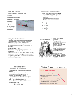
ϕ=−
r
α
This potential is plotted in Fig. 3. One observes that it markedly deviates from the Newtonian potential of general relativity. The most striking feature is that the gravitational force
becomes repulsive at distances r > 1/mg . At large distances the potential goes to zero. This
is different from the case of massive gravities with gapless field φ0 [5], where the gravitational
potential generically presents linear growth with distance21 [52, 34]. Note also that there
25
ϕ
ϕmax
0
2m −1
g
m−1
kh
r
Figure 3: The shape of the Newton potential in the massive gravity model of this paper.
The gravitational force becomes repulsive at distances larger than the inverse graviton mass.
is no van Dam–Veltman–Zakharov (vDVZ) discontinuity [56, 57]: in the limit µ → 0 the
potentials ϕ, Ψ reduce to their GR expressions.
To understand the behavior of the Newton potential in more detail, we expand the
√
−1
exponent at r ≪ ckh m−1
kh = ( αmg ) . At these distances the khronon mass is irrelevant
and one expects the potential to coincide with the results existing in the literature. We
obtain,
r
m2g r
2
1
mg −
+ ... ,
(87)
ϕ = GN M⊙ − +
r
α
2
√
where dots stand for the terms that are suppressed by the powers of the combination αmg r.
The second term in brackets gives a constant shift of the Newton potential which drops off
from the observables involving only distances r . 1/mg . The third term gives precisely
the linear contribution discussed in [52, 34]. Note that for our model this contribution is
√
repulsive. The potential reaches a maximum at r = 2/mg where
ϕmax =
p
2/α GN M⊙ mg .
For the validity of the linearized approximation ϕmax must be much smaller than one.
This translates into the condition that the graviton mass must be smaller than the in√
verse Schwarzschild radius of the source multiplied by α. Unless α is extremely small, this
condition is not very restrictive.
21
This growth may be cut by non-linearities of the model [5, 54, 55] or by non-stationary evolution of the
background [34]. Also, it is absent if the coefficients in the mass term (6) satisfy certain relations [5, 52].
26
Stronger phenomenological constraints come from the requirement that the gravitational
field of localized sources should not significantly deviate from the standard form at astrophysical scales. The Solar System tests put a limit on the difference between the two gravitational
potentials ϕ and Ψ. In the post-Newtonian (PPN) framework this is traditionally parameterized by the ratio γ ≡ Ψ/ϕ and the current constraint (measured at the orbit of Saturn
by the Cassini satellite) reads [58],
γ − 1 = (2.1 ± 2.3) × 10−5 .
(88)
From the expressions22 (84), (87) we obtain the formula for γ in our model at distances
shorter than inverse khronon mass,
γ =1−
(mg r)2
.
2
(89)
This gives an upper bound mg < 4 × 10−17 cm−1 ∼ 120 pc−1 . A tighter limit comes from
the gravitational field of galaxies. The requirement that it matches the standard expression
implies
mg . (1 Mpc)−1 .
(90)
It is likely that yet stronger bounds can be obtained from the large scale structure and the
cosmic microwave background (CMB). We leave this analysis for future.
It would be also interesting to explore if the gravitational repulsion found above can be
active at the cosmological scales and lead to accelerated expansion of the universe. Note
that this mechanism of acceleration would rely crucially on the presence of inhomogeneities,
as the homogeneous FRW Ansatz does not exhibit any self-accelerated behavior (see Sec. 4).
Before closing this section, let us mention that a complementary way to constrain the
graviton mass is by looking directly at the modifications in the helicity-2 sector. These
have consequences for radiation and propagation of gravity waves [52, 59, 60]. Having a
more complete theory allows to put these studies on the firm ground in the situations with
characteristic scales smaller than Λ−1
2 , such as inflation and reheating.
7
Summary and discussion
In this paper we have proposed an embedding of Lorentz violating massive gravity above
p
the scale Λ2 ≡ mg MP . The proposed theory has a high cutoff scale only a few orders of
magnitude below the Planck mass and independent of the mass of the graviton. At high
22
We subtract the constant piece from (87).
27
energies the theory possesses a large symmetry FDiff × SO(3) which is spontaneously broken
at lower energy to a diagonal global SO(3) subgroup. This pattern of symmetry breaking
is realized by a triplet of space-like vector fields which develop non-zero VEVs. A crucial
technical role is played by a quadratic mixing between the vectors and the St¨
uckelberg fields
a
φ of massive gravity. Once the vectors acquire VEVs, this mixing forces the St¨
uckelbergs to
develop coordinate-dependent profiles, which eventually translates into the graviton mass.
This means that no non-linear interactions in the Stuckelberg sector are required to do this
job and one can restrict to purely quadratic action for the fields φa , thus eliminating any
strong coupling from this sector. This mechanism is reminiscent of the proposal for the
(partial) UV completion of the ghost condensate model [47, 36] where a mixing between a
time-like vector acquiring a VEV and a massless scalar forces the latter to evolve in time.
The graviton mass in the model is proportional to the product of the vector VEVs and
the coefficient in front of the vector-St¨
uckelberg mixing. Thus, it vanishes both if the vector
VEVs disappear (in the unbroken phase) or if the mixing is switched off. The action stays
regular in the limit of vanishing mass and therefore one expects all observable quantities,
with the quantum corrections included, to behave smoothly in this limit. In this sense our
mechanism is analogous to the Higgs mechanism of gauge theories. It is worth stressing that
in our model the mixing between the vector and St¨
uckelberg fields is protected by a discrete
a
a
symmetry φ 7→ −φ and thus a small coefficient in front of it is technically natural. This
implies that the graviton mass is stable under quantum corrections.
We analyzed the structure of the theory at different energies and explicitly verified the
expectation that new degrees of freedom, besides those of pure massive gravity, must exist
below the scale Λ2 . Indeed, we found that certain components of the vector fields propagate
at these energies. These degrees of freedom have a mass gap which is parametrically smaller
than Λ2 , but still bigger than mg . It would be interesting to work out the consequences of
these new light degrees of freedom for phenomenology.
We also found that the helicity-0 component of the graviton, which in our model is
identified with the khronon of the khronometric model, acquires a mass parametrically lower
than mg . This has important implications for the gravitational potentials of localized sources:
unlike previous models of LV massive gravity, in our case the potentials fall of exponentially
at large distances. Remarkably, the shape of the Newton potential is not monotonic. It
grows from negative values at short distances, changes sign, reaches a positive maximum at
√
r = 2m−1
g and then decreases towards r → ∞. This implies that the gravitational force
√
becomes repulsive at r > 2m−1
g . This property may lead to a rich phenomenology which
we leave for future studies. An interesting question is whether the gravitational repulsion
28
between the inhomogeneities present in the universe can provide the accelerated expansion
at recent epoch, despite the fact that for the strictly homogeneous Ansatz our model does
not exhibit any self-acceleration.
A subtle theoretical aspect of our model, inherited from the effective theory of LV massive gravity, is the presence of instantaneous interactions. We have addressed the issue of
quantization of the instantaneous modes and argued that it can be performed consistently.
We also pointed out that in the canonical formalism the instantaneous modes must be interpreted as a certain type of non-locality along the spatial dimensions. To make the discussion
concise, we focused on simplified toy models. A more comprehensive study of this topic is
definitely required owing to its importance for LV proposals for quantum gravity [23, 25].
Another open question left for future research is to understand how the strong coupling of
LV massive gravity manifests itself at the level of Feynman diagrams and how it is canceled
by the new degrees of freedom appearing in our model (see [32, 61] for related works in the
Lorentz invariant context). This may shed light on possible generalizations of the mechanism
proposed in this paper to other IR modifications of gravity, such as multi-metric theories
and the Lorentz invariant setup of [7]. In particular, it would be interesting to prove at the
diagrammatic level the (im)possibility of a Lorentz invariant Wilsonian UV completion of
the latter setup.
Acknowledgments
We are grateful to Denis Comelli, Sergei Dubovsky, Maxim Pospelov and Mikhail Ivanov
for useful discussions. We also thank Claudia de Rham and Gregory Gabadadze for useful
comments on the draft. S.S. is grateful to the Perimeter Institute for hospitality during
this work. Research at Perimeter Institute is supported by the Government of Canada
through Industry Canada and by the Province of Ontario through the Ministry of Economic
Development & Innovation.
References
[1] M. Fierz and W. Pauli, Proc. Roy. Soc. Lond. A 173 (1939) 211.
[2] D. G. Boulware and S. Deser, Phys. Rev. D 6 (1972) 3368.
[3] P. Creminelli, A. Nicolis, M. Papucci and E. Trincherini, JHEP 0509 (2005) 003 [hepth/0505147].
29
[4] V. A. Rubakov, “Lorentz-violating graviton masses: Getting around ghosts, low strong
coupling scale and VDVZ discontinuity,” hep-th/0407104.
[5] S. L. Dubovsky, JHEP 0410, 076 (2004) [hep-th/0409124].
[6] V. A. Rubakov and P. G. Tinyakov, Phys. Usp. 51 (2008) 759 [arXiv:0802.4379 [hep-th]].
[7] C. de Rham, G. Gabadadze and A. J. Tolley, Phys. Rev. Lett. 106 (2011) 231101
[arXiv:1011.1232 [hep-th]].
[8] K. Hinterbichler, Rev. Mod. Phys. 84 (2012) 671 [arXiv:1105.3735 [hep-th]].
[9] C. de Rham, Living Rev. Rel. 17, 7 (2014) [arXiv:1401.4173 [hep-th]].
[10] C. de Rham, G. Gabadadze, L. Heisenberg and D. Pirtskhalava, Phys. Rev. D 87,
085017 (2013) [arXiv:1212.4128].
[11] C. de Rham, L. Heisenberg and R. H. Ribeiro, Phys. Rev. D 88, 084058 (2013)
[arXiv:1307.7169 [hep-th]].
[12] N. Kaloper, A. Padilla, P. Saffin and D. Stefanyszyn, “Unitarity and the Vainshtein
Mechanism,” arXiv:1409.3243 [hep-th].
[13] M. Porrati, JHEP 0204, 058 (2002) [hep-th/0112166]; Mod. Phys. Lett. A 18, 1793
(2003) [hep-th/0306253].
[14] E. Kiritsis, JHEP 0611 (2006) 049 [hep-th/0608088].
[15] O. Aharony, A. B. Clark and A. Karch, Phys. Rev. D 74 (2006) 086006 [hep-th/0608089].
[16] D. Blas, “Aspects of Infrared Modifications of Gravity,” arXiv:0809.3744 [hep-th].
[17] A. Joyce, B. Jain, J. Khoury and M. Trodden, “Beyond the Cosmological Standard
Model,” arXiv:1407.0059 [astro-ph.CO].
[18] D. Vegh, “Holography without translational symmetry,” arXiv:1301.0537 [hep-th].
[19] M. Blake, D. Tong and D. Vegh, Phys. Rev. Lett. 112 (2014) 071602 [arXiv:1310.3832
[hep-th]].
[20] N. Arkani-Hamed, H. Georgi and M. D. Schwartz, Annals Phys. 305 (2003) 96 [hepth/0210184].
30
[21] D. T. Son, Phys. Rev. Lett. 94 (2005) 175301 [cond-mat/0501658].
[22] S. Dubovsky, T. Gregoire, A. Nicolis and R. Rattazzi, JHEP 0603 (2006) 025 [hepth/0512260].
[23] P. Horava, Phys. Rev. D 79, 084008 (2009) [arXiv:0901.3775 [hep-th]].
[24] B. Cuadros-Melgar, E. Papantonopoulos, M. Tsoukalas and V. Zamarias, Phys. Rev. D
85 (2012) 124035 [arXiv:1108.3771 [hep-th]].
[25] D. Blas, O. Pujolas and S. Sibiryakov, JHEP 1104, 018 (2011) [arXiv:1007.3503 [hepth]].
[26] A. Gruzinov, “All Fierz-Paulian massive gravity theories have ghosts or superluminal
modes,” arXiv:1106.3972 [hep-th].
[27] C. Burrage, C. de Rham, L. Heisenberg and A. J. Tolley, JCAP 1207, 004 (2012)
[arXiv:1111.5549 [hep-th]].
[28] S. Deser, M. Sandora, A. Waldron and G. Zahariade, “Covariant constraints for generic
massive gravity and analysis of its characteristics,” arXiv:1408.0561 [hep-th].
[29] A. Adams, N. Arkani-Hamed, S. Dubovsky, A. Nicolis and R. Rattazzi, JHEP 0610,
014 (2006) [hep-th/0602178].
[30] Z. Berezhiani, D. Comelli, F. Nesti and L. Pilo, Phys. Rev. Lett. 99 (2007) 131101
[hep-th/0703264 [HEP-TH]].
[31] D. Blas, C. Deffayet and J. Garriga, Phys. Rev. D 76 (2007) 104036 [arXiv:0705.1982
[hep-th]].
[32] M. D. Schwartz, Phys. Rev. D 68 (2003) 024029 [hep-th/0303114].
[33] N. Arkani-Hamed, H. -C. Cheng, M. A. Luty and S. Mukohyama, JHEP 0405, 074
(2004) [hep-th/0312099].
[34] D. Blas, D. Comelli, F. Nesti and L. Pilo, Phys. Rev. D 80 (2009) 044025
[arXiv:0905.1699 [hep-th]].
[35] N. Arkani-Hamed, H. C. Cheng, M. A. Luty, S. Mukohyama and T. Wiseman, JHEP
0701 (2007) 036 [hep-ph/0507120].
31
[36] M. M. Ivanov and S. Sibiryakov, JCAP 1405, 045 (2014) [arXiv:1402.4964 [astroph.CO]].
[37] G. Gabadadze and L. Grisa, Phys. Lett. B 617, 124 (2005) [hep-th/0412332].
[38] L. Shao, R. N. Caballero, M. Kramer, N. Wex, D. J. Champion and A. Jessner, Class.
Quant. Grav. 30, 165019 (2013) [arXiv:1307.2552 [gr-qc]].
[39] K. Yagi, D. Blas, N. Yunes and E. Barausse, Phys. Rev. Lett. 112, 161101 (2014)
[arXiv:1307.6219 [gr-qc]]; Phys. Rev. D 89, 084067 (2014) [arXiv:1311.7144 [gr-qc]].
[40] D. Blas, O. Pujolas and S. Sibiryakov, Phys. Rev. Lett. 104 (2010) 181302
[arXiv:0909.3525 [hep-th]].
[41] D. Benedetti and F. Guarnieri, JHEP 1403, 078 (2014) [arXiv:1311.6253 [hep-th]].
[42] G. D’Odorico, F. Saueressig and M. Schutten, “Asymptotic freedom in Horava-Lifshitz
gravity,” arXiv:1406.4366 [gr-qc].
[43] M. C. Bento, O. Bertolami, P. V. Moniz, J. M. Mourao and P. M. Sa, Class. Quant.
Grav. 10, 285 (1993) [gr-qc/9302034].
[44] C. Armendariz-Picon, JCAP 0407, 007 (2004) [astro-ph/0405267].
[45] M. V. Libanov and V. A. Rubakov, JHEP 0508, 001 (2005) [hep-th/0505231].
[46] D. S. Gorbunov and S. M. Sibiryakov, JHEP 0509, 082 (2005) [hep-th/0506067];
arXiv:0804.2248 [hep-th].
[47] D. Blas and S. Sibiryakov, JCAP 1107 (2011) 026 [arXiv:1104.3579 [hep-th]].
[48] T. Brauner, Symmetry 2 (2010) 609 [arXiv:1001.5212 [hep-th]].
[49] A. Nicolis and F. Piazza, Phys. Rev. Lett. 110 (2013) 011602 [arXiv:1204.1570 [hep-th]].
[50] H. Watanabe and H. Murayama, Phys. Rev. Lett. 108 (2012) 251602 [arXiv:1203.0609
[hep-th]].
[51] S. Liberati, Class. Quant. Grav. 30 (2013) 133001 [arXiv:1304.5795 [gr-qc]].
[52] S. L. Dubovsky, P. G. Tinyakov and I. I. Tkachev, Phys. Rev. Lett. 94 (2005) 181102
[hep-th/0411158]; Phys. Rev. D 72, 084011 (2005) [hep-th/0504067].
32
[53] D. Blas, O. Pujolas and S. Sibiryakov, JHEP 0910 (2009) 029 [arXiv:0906.3046 [hepth]].
[54] M. V. Bebronne and P. G. Tinyakov, JHEP 0904, 100 (2009) [Erratum-ibid. 1106, 018
(2011)] [arXiv:0902.3899 [gr-qc]].
[55] D. Comelli, F. Nesti and L. Pilo, Phys. Rev. D 83 (2011) 084042 [arXiv:1010.4773
[hep-th]].
[56] H. van Dam and M. J. G. Veltman, Nucl. Phys. B 22, 397 (1970).
[57] V. I. Zakharov, JETP Lett. 12, 312 (1970) [Pisma Zh. Eksp. Teor. Fiz. 12, 447 (1970)].
[58] C. M. Will, Living Rev. Rel. 17, 4 (2014) [arXiv:1403.7377 [gr-qc]].
[59] S. Dubovsky, R. Flauger, A. Starobinsky and I. Tkachev, Phys. Rev. D 81 (2010) 023523
[arXiv:0907.1658 [astro-ph.CO]].
[60] S. Mirshekari, N. Yunes and C. M. Will, Phys. Rev. D 85 (2012) 024041 [arXiv:1110.2720
[gr-qc]].
[61] A. Aubert, Phys. Rev. D 69 (2004) 087502 [hep-th/0312246].
33