Technical Solution for Reducing the
Dynamic Interaction Soil-Foundation
Slimane Benayad
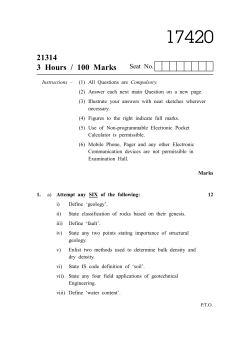
Department of Civil Engineering, University of Bechar, Algeria
e-mail: [email protected]
Abdelmadjid Berga
Department of Civil Engineering, University of Bechar, Algeria
e-mail: [email protected]
Nazihe Terfaya
Department of Mechanical Engineering, University of Bechar, Algeria
e-mail: [email protected]
ABSTRACT
The objective of this paper is to model the transfer of vibrations in a rigid soil and to find a
way to reduce the response to these vibrations. We propose a new technique that involves
building a deep uncompressed soil layer in a peripheral trench. The trench is dug around
structures to absorb the deformations of the soil and thus reduce the stresses in structures.
Using the (2D) PLAXIS software, a finite element numerical modeling is used taking into
account the soil-foundation interaction and with a dynamic resolution based on the Newmark
method, which remains the most used second order implicit method. Some results and
conclusions regarding the movements and ground speeds are also presented.
KEYWORDS:
soil; structure; interactions; dynamics; finite element method.
INTRODUCTION
Some landslides may have different origins (natural anthropic collapses of underground
cavities, ore mining, pumping water, gas exploration and hydrocarbon vibration machines, etc.).
These movements may exceed certain thresholds characterizing the eligible behavior of
structures, and cause damage and destruction of buildings ranging from the damage of
infrastructure to losses of life, and therefore limit the economic and social development. Ground
deformations cause damage that is transmitted to structures in two modes (a push or a loosening
of the ground and friction along the interface between the structure and land. The level of damage
depends on the characteristics of soil geo-mechanical and geometrical characteristics of the
structure and properties of interfaces.
Using the (2D) PLAXIS software, a two-dimensional modeling and nonlinear finite element
method is used. We also present a comparison of results to choose the best dimensioning of the
trench.
MODELING THE PROPAGATION OF VIBRATIONS
Understanding on-site vibration measurements is partially possible by means of a mechanical
analysis of phenomena (in terms of values of velocity, acceleration, displacement, strain, stress,
etc.). Confrontation of such an analysis with experimental data provides an initial interpretation of
- 6583 -
Vol. 19 [2014], Bund. V
6584
these vibrations. However, field data are often lacking; only orders of magnitude are generally
available. Indeed, the attenuation or amplification of the vibratory movement and changes in the
frequency content of the wave field on the propagation path depend on the modules (or wave
velocities) and on depreciation in the layers and their respective thicknesses. In addition, within
complex geometric configurations, mechanical models escape an exact resolution and it is,
therefore, necessary to consider numerical simulations.
Theoretical Modeling of Mitigation
From a signal measured at the distance xi from the source, the acceleration distance x j can be
estimated in the frequency domain, using the following equation (Semblat & Pecker, 2009):
[
a * ( x j , ω ) = a * ( xi , ω ) exp ik * (ω )( x j − xi )
]
(1)
where a * ( x, ω ) represents the Fourier acceleration spectrum measured at the distance x and
k * (ω ) the complex wave number defined by (Aki & Richards, 1980):
k * (ω ) = k (ω ) − iα (ω )
(2)
where k (ω ) = 2πc / ω is the real wave number (proportional to the velocity c of the wave) and
the attenuation factor (Bourbié, Coussy & Richards, 1986).
Theoretical Modeling of Amplification
In the seismic field, it is shown that a wave can be greatly amplified when the contrast of
celerity between soil layers is important (Semblat & Pecker, 2009), (Semblat, Duval & Dangla,
2000), (Semblat & Dangla, 2005). So we recall here how the amplification of a shear wave in a
layer of soil can be described in the simple case of a homogeneous layer of constant thickness
(Figure 1). It is possible to calculate the wave propagating in the layer and into the underlying
soil.
Figure 1: Amplification of a plane wave in a layer of soil
Vol. 19 [2014], Bund. V
6585
In each medium, the displacement resulting from the superposition of waves traveling
upwards (z > 0) and downwards (z < 0) is written by choosing the origin of the z-axis at the top of
each layer (Semblat & Pecker, 2009), (Aki & Richards, 1980)
[
]
u n = An exp(ik zn z n ) + An′ exp(−ik zn z n ) f n ( x, t )
(3)
where the vertical wave number in the layer n is defined by:
k zn =
ω cos θ n
v sn
 iω

f n ( x, t ) = exp  ( x sin θ n − v sn t )
 v sn

(4)
(5)
With v sn as shear wave velocity θ n and impact in the layer n.
The index n equals 1 for the surface layer and 2 for the underlying soil. An and An′ are the
amplitudes of the waves propagating respectively upwards and downwards in the n-layer.
METHODOLOGY AND DYNAMIC ANALYSIS
The equilibrium equation that governs the dynamic response of a system can be written:
 + CU
 + KU = F ext
MU
(6)
M : The mass matrix.
C : The damping matrix.
K : The stiffness matrix.
 , U
 , U : Respectively, the vectors of the accelerations, velocities and displacements
U
F ext : The vector of external load acting on the entire structure
The Newmark Schema
Newmark's method is a direct method for solving equations of dynamic equilibrium. It is
based on the following approximations: on the displacements and velocities at the t + ∆t moment
based on the displacements, velocities and accelerations at the moments t + ∆t and t as follows
(Bathe & Wilson, 1976), (Bathe, 1996):
 t + αu
 t + ∆t ]
u t + ∆t = u t + ∆t [(1 − α )u
u t + ∆t = u t + ∆tu t +
∆t 2
 t + 2 βu
 t + ∆t ]
+ [(1 − 2 β )u
2
(7)
(8)
Vol. 19 [2014], Bund. V
6586
Parameters α and β must be chosen depending on given applications. These parameters
determine the details and the convergence of the algorithm. By injecting the approximations (7)
and (8) in the equilibrium equation (6), we obtain an equation where the only unknown is the
displacement.
with a 0 =
KU t + ∆t = Ft + ∆t
(9)
K = K + a 0 M + a1C
(10)



 +a U
Ft + ∆t = Ft + ∆t + M (a0 U t + a 2 U
t
3 t ) + C(a1 U t + a 4 U t + a 5 U t )
(11)
β
1
1
1
∆t  β
β

− 1 , a 4 = − 1 , a5 =  − 2  .
, a1 =
, a2 =
, a3 =
2
α
∆t
α∆t
2α
2 α
α∆t

Velocities and accelerations are updates at the end not by the expressions:



U
t + ∆t = a 0 (U t + ∆t − U t ) − a 2 U t − a 3 U t
(12)




U
t + ∆t = U t + a 6 U t + a 7 U t + ∆t
(13)
with, a 6 = α∆t , a 7 = ∆t (1 − β ) .
Incremental Form
Assuming that the equilibrium equation is verified at t moment and if we consider the
decomposition of accelerations, velocities and displacements as follows:



U
t + ∆t = U t + ∆U

 + ∆U

U t + ∆t = U
t
U
 t + ∆t = U t + ∆U
(14)

 , ∆U and ∆U respectively show the variations of the accelerations,
where the terms ∆U
velocities and displacements during the time increment ∆t , where the dynamic equation (6) takes
the form:
(
 + ∆U
 ) + C(U
 + ∆U
 ) + K (U + ∆U ) = F ext + ∆F ext
M (U
t
t
t
)
(15)
which gives:
 + C∆U
 + K∆U = ∆F ext
M∆U
(16)
Using the expressions (12), (13) of acceleration and speed at the t + ∆t moment according to
the movements of time t + ∆t , we can express the accelerations and incremental velocities based
on incremental movements:
 = a ∆U − a U


∆U
0
2 t − (1 − a 3 )U t
(17)
 = (a + a )U
 + a ∆U

∆U
6
7
t
7
(18)
Vol. 19 [2014], Bund. V
6587
By substituting the expressions (15), (16) in equation (14) we obtain the following equation:
K∆U = ∆F
(19)
K = K + a0 M + a7 a0 C
(20)
where:
and
(
) (
 − (1 − a )U
 + C (a + a )U
 − a a U

∆F = ∆F + M − a 7 a 2 U
t
3
t
3
6
t
7 2 t
)
(21)
Newmark's method is rewritten in an incremental form. The field ∆U representative of the
variation of displacement during an increment of time ∆t becomes the new unknown.
At the end of the step, equations (14) can update the displacements, velocities, accelerations,
and reactions.
In its original version, Newmark proposed values α = 0.5 and β = 0.25 that correspond to
the rules of a trapezoid. These values allow to have stability of the linear problem. The result was
generalized and the stability condition is provided for β ≥
Wilson, 1976).
2
11
1

and α ≥  + β  (Bathe &
42
2

NUMERICAL MODEL
In this example we consider an elasto-plastic (Mohr-Coulomb criterion) for soil and elastic
behavior for the foundation. Physical and geometric characteristics with boundary conditions of
the soil and the foundation are presented in Figure 2, and Table 1 and Table 2.
Machine: f = 30 Hz
Amplitude = 30 kN/m2
Figure 2: Geometric properties and boundary conditions
Vol. 19 [2014], Bund. V
6588
Table 1: Properties of soil layers and interface
Parameters
Name
Model type
Type de comportement
Rigid Soil
Model
Type
γ dry
γ wet
Dry unit weight
Humid unit weight
Horizontal permeability
Vertical permeability
Young Module
Poisson coefficient
Kx
Ky
Eref
ν
c ref
ϕ
ψ
Cohesion
Friction Angle
Dilatation angle
Rigidity Factor of the interface
Rinter
Trench layer
Unit
Mohr-coulomb
Drain
Mohr-coulomb
Drain
-
17
16
kN/m3
19
1,157E-06
1,157E-06
2,000E+04
0,330
20
1,157E-06
1,157E-06
2000,000
0,300
kN/m3
m/jour
m/jour
kN/m2
-
8
29
0
1
1
30
0
1
kN/m3
°
°
-
Table 2: Properties of the sole
Parameters
Type of behaviour
Normal rigidity
Flexual rigidity
Equivalent thickness
Weights
Poisson coefficient
Name
Material type
EA
EI
d
w
Foundation
Elastic
7,600E+06
2,400E+04
0,195
5,000
0
ν
kN/m
kNm2/m
m
kN/m/m
-
Unit
INTERPRETATION AND CONCLUSION
0,025
Without trench (H=0)
H=1m
H=4m
H=8m
Displacements (m)
0,020
0,015
0,010
0,005
0,000
0,0
0,2
0,4
0,6
0,8
1,0
Time (s)
Figure 3: Effect of the depth (H) of the trench on the displacements (L = 2 m)
Vol. 19 [2014], Bund. V
6589
0,040
Without trench (H=0m)
H=8m
0,035
0,030
velocities (m/s)
0,025
0,020
0,015
0,010
0,005
0,000
-0,005
0,0
0,2
0,4
0,6
0,8
1,0
time (s)
Figure 4: Effect of the depth (H) of the trench on the velocities (L = 2m)
0,025
Without trench (L=0m)
L=1m
L=2m
Displacements (m)
0,020
0,015
0,010
0,005
0,000
0,0
0,2
0,4
0,6
0,8
1,0
Time (s)
Figure 5: Effect of the width (L) of the trench on the displacements (H = 6 m)
Vol. 19 [2014], Bund. V
6590
0,040
0,035
Velocities (m/s)
0,030
0,025
0,020
0,015
Without trench (L=0m)
(L=1m)
(L=2m)
0,010
0,005
0,000
0,0
0,2
0,4
0,6
0,8
1,0
Time (s)
Figure 6: Effect of the width (L) of the trench on the velocities (H m = 6)
It can be clearly observed from the obtained graphs of displacement and velocity (Figure 3, 4,
5, 6) that:
-
The greater the width (L) and depth (H) of the trench, the more the displacements and
velocities decrease.
-
One can also notice the velocity reduction which implies the reduction in acceleration.
-
The percentage decrease of the displacement and velocity being 29% for the increase of the
depth (H) and 47% for the increase in the width (L). Indicating that most affects the width
than depth. This justifies the validity of the proposed technique to reduce the transmission of
vibration and minimize their impact on the adjoining structures.
REFERENCES
1. Aki, K. and P. G. Richards (1980) “Quantitative Seismology, Theory and
Methods,” Vol. I and II, W.H. Freeman. San Francisco.
2. Bathe, K. J. and E. L. Wilson (1976) “Numerical methods in finite element analysis,”
Prentice-Hall Inc., USA , pp. 458-460.
3. Bathe. K. J. (1996) “Finite element procedures,” Englewood Cliffs. NJ. PrenticeHall.
4. Bourbié, T., O. Coussy and B. Zinszner (1986) “Acoustique Des Milieux Poreux,”
Editions Technip. Paris.
5. Semblat, J.F., A. M. Duval and P. Dangla (2000) “Numerical analysis of seismic
wave amplification in Nice (France) and comparisons with experiments,” Soil
Dynamics and Earthquake Engineering. 19(5), pp.347-362.
Vol. 19 [2014], Bund. V
6591
6. Semblat, J.F. and P. Dangla (2005) “Modélisation de la propagation d’ondes et de
l’interaction sol-structure : approches par éléments finis et éléments de frontière,”
Bulletin des Laboratoires des Ponts et Chaussées, No.256-257, pp. 163-178.
7. Semblat, J. F. and A. Pecker (2009) “Waves and Vibrations in Soils: Earthquakes,
Traffic, Shocks, Construction Works,” IUSS Press. Pavia, Italy., 500 pages.
© 2008 ejge