
AADL Fault Modeling and Analysis Within an ARP4761 Safety Assessment Julien Delange
AADL Fault Modeling and Analysis Within an ARP4761 Safety Assessment Julien Delange Peter Feiler David P. Gluch John Hudak October 2014 TECHNICAL REPORT CMU/SEI-2014-TR-020 Software Solutions Division http://www.sei.cmu.edu Copyright 2014 Carnegie Mellon University This material is based upon work funded and supported by the Department of Defense under Contract No. FA8721-05-C-0003 with Carnegie Mellon University for the operation of the Software Engineering Institute, a federally funded research and development center. Any opinions, findings and conclusions or recommendations expressed in this material are those of the author(s) and do not necessarily reflect the views of the United States Department of Defense. This report was prepared for the SEI Administrative Agent AFLCMC/PZM 20 Schilling Circle, Bldg 1305, 3rd floor Hanscom AFB, MA 01731-2125 NO WARRANTY. THIS CARNEGIE MELLON UNIVERSITY AND SOFTWARE ENGINEERING INSTITUTE MATERIAL IS FURNISHEDON AN “AS-IS” BASIS. CARNEGIE MELLON UNIVERSITY MAKES NO WARRANTIES OF ANY KIND, EITHER EXPRESSED OR IMPLIED, AS TO ANY MATTER INCLUDING, BUT NOT LIMITED TO, WARRANTY OF FITNESS FOR PURPOSE OR MERCHANTABILITY, EXCLUSIVITY, OR RESULTS OBTAINED FROM USE OF THE MATERIAL. CARNEGIE MELLON UNIVERSITY DOES NOT MAKE ANY WARRANTY OF ANY KIND WITH RESPECT TO FREEDOM FROM PATENT, TRADEMARK, OR COPYRIGHT INFRINGEMENT. This material has been approved for public release and unlimited distribution except as restricted below. Internal use:* Permission to reproduce this material and to prepare derivative works from this material for internal use is granted, provided the copyright and “No Warranty” statements are included with all reproductions and derivative works. External use:* This material may be reproduced in its entirety, without modification, and freely distributed in written or electronic form without requesting formal permission. Permission is required for any other external and/or commercial use. Requests for permission should be directed to the Software Engineering Institute at [email protected]. * These restrictions do not apply to U.S. government entities. Carnegie Mellon® is registered in the U.S. Patent and Trademark Office by Carnegie Mellon University. DM-0000593 Table of Contents Acknowledgments ix Abstract xi 1 Introduction 1.1 Functional Hazard Assessment 1.2 Preliminary System Safety Assessment 1.3 System Safety Assessment 1.4 Reader’s Guide 1 2 2 3 3 2 AADL Error Model Constructs That Support ARP4761 2.1 Error Propagation 2.1.1 Definition 2.1.2 Procedure 2.1.3 Constraints 2.1.4 Example 2.2 Error Source 2.2.1 Definition 2.2.2 Procedure 2.2.3 Constraints 2.2.4 Example 2.3 Error Path 2.3.1 Definition 2.3.2 Procedure 2.3.3 Constraints 2.3.4 Examples 2.4 Error Sink 2.4.1 Definition 2.4.2 Procedure 2.4.3 Example 2.5 Error Events 2.5.1 Definition 2.5.2 Procedure 2.5.3 Constraints 2.5.4 Example 2.6 Error States 2.6.1 Definition 2.6.2 Procedure 2.6.3 Constraints 2.6.4 Example 2.7 Error Transitions 2.7.1 Definition 2.7.2 Procedure 2.7.3 Constraints 2.7.4 Example 2.8 Error Propagation Condition 2.8.1 Definition 2.8.2 Procedure 2.8.3 Constraints 2.8.4 Example 4 4 4 5 5 5 8 8 8 8 8 9 9 10 10 10 12 12 12 12 13 13 13 13 13 14 14 14 14 14 15 15 15 15 16 16 16 16 17 17 CMU/SEI-2014-TR-020 | i 2.9 Composite Error Behavior Model 2.9.1 Definition 2.9.2 Procedure 2.9.3 Constraints 2.9.4 Example 2.10 Hazards Property 2.10.1 Definition 2.10.2 Procedure 2.10.3 Constraints 2.10.4 Example 2.11 OccurrenceDistribution Property 2.11.1 Definition 2.11.2 Procedure 2.11.3 Constraints 2.11.4 Example 17 17 17 18 18 19 19 21 21 21 22 22 23 23 23 3 OSATE Tool Set 3.1 Functional Hazard Assessment Support 3.1.1 Processed Modeling Patterns 3.1.2 Example Model 3.1.3 Fault and Hazard Analysis Report Example 3.2 Fault Tree Analysis Support 3.2.1 Introduction 3.2.2 Using the Fault Tree Analysis Generator 3.2.3 Mapping to OpenFTA Format File 3.2.4 Mapping to Generic XML Format 3.2.5 AADL and FTA Mapping Rules 3.2.6 Issues and Known Limitations 3.3 Failure Modes and Effects Analysis Support 3.4 Dependence and Reliability Block Diagram Support 3.4.1 Introduction 3.4.2 Processed Modeling Patterns 3.4.3 Algorithm 3.4.4 Example 3.4.5 Known Issues and Limitations 3.5 Markov Analysis Support 3.5.1 Continuous-Time Markov Chains 3.5.2 Discrete-Time Markov Chains 3.5.3 AADL Export to PRISM Function 3.5.4 AADL and PRISM Mapping Rules 3.5.5 Issues and Known Limitations 3.6 Error-Model Consistency 3.7 Unhandled Faults 24 24 25 25 26 27 27 27 27 28 28 29 30 31 31 32 33 34 37 37 37 39 41 42 43 43 45 4 Wheel Brake System Example 4.1 Overview 4.1.1 Wheel Brake System Architecture 4.1.2 Safety Evaluation Materials 4.2 Simple Model 4.2.1 Overview 4.2.2 Adding Faults and Errors Information in the AADL Model 4.2.3 Functional Hazard Assessment 4.2.4 Fault Tree Analysis 4.2.5 Failure Modes and Effects Analysis 47 47 48 48 49 49 51 56 57 58 CMU/SEI-2014-TR-020 | ii 4.3 5 Advanced Model 4.3.1 Overview 4.3.2 Functional Model 4.3.3 Realization Model 4.3.4 Binding Realization and Functional Models Summary 59 59 60 61 62 67 Acronyms 68 References 69 CMU/SEI-2014-TR-020 | iii CMU/SEI-2014-TR-020 | iv List of Figures Figure 1: Overview of the Safety Assessment Process [SAE 1996] 1 Figure 2: Basic Dual-Redundant Control System 5 Figure 3: Error Propagation from Controller 1 7 Figure 4: Graphical Representation of the Control System with Error Flows 11 Figure 5: Error Flow of the HardwareFailure to SoftwareFailure Using Bindings 11 Figure 6: OSATE Functions for Consistency Analysis 24 Figure 7: OSATE’s Functional Hazard Assessment Report 26 Figure 8: Error State for the Fault Tree Analysis 27 Figure 9: OSATE’s Reports Subdirectory 27 Figure 10: Fault Tree Analysis as Shown in OpenFTA 28 Figure 11: Fault Analyses Menu in OSATE 30 Figure 12: File Hierarchy Containing Error-Related Reports 30 Figure 13: Redundant Controller Architecture RBD 31 Figure 14: Combined RBD 32 Figure 15: RBD Results 34 Figure 16: Graphical Instance Model for the RBD Analysis 35 Figure 17: Result of the Plug-in on the RBD Analysis 35 Figure 18: Dual-Sensor Model with No Repair 37 Figure 19: Dual-Sensor Model with Repair 38 Figure 20: Graphical Output of the PRISM Simulation 39 Figure 21: DTMC State Diagram 40 Figure 22: Selection of the Markov-Chain Type 42 Figure 23: Files Hierarchy and the Produced PRISM File 42 Figure 24: Report of Unhandled Error Types in Eclipse Problems View 46 Figure 25: Files Hierarchy of the Model 49 Figure 26: Overview of the Complete Model of the WBS 50 Figure 27: Variation of the BSCU Implementation 51 Figure 28: Error Paths from the Battery to Select_Alternate 54 Figure 29: Extract of the Functional Hazard Assessment 57 Figure 30: Extract of the Fault Tree Analysis 58 Figure 31: Extract of the FMEA 58 Figure 32: Functional Model 60 Figure 33: Decomposition of the Decelerate Function 61 CMU/SEI-2014-TR-020 | v Figure 34: Realization Model 62 Figure 35: Example of Binding a Functional and a Realization Model 63 Figure 36: Fault Impact Analysis of the Functional Model 66 Figure 37: Fault Impact Analysis for the Integrated Model (Implementation + Functional) 66 CMU/SEI-2014-TR-020 | vi List of Tables Table 1: ARP4761 Process Elements and Supporting AADL Error Model Constructs 4 Table 2: RBD Failure Rate Equations 32 Table 3: Composite System Error Behavior for a Redundant Control System Architecture 33 Table 4: Mapping Rules for the AADL to PRISM Transformation 42 CMU/SEI-2014-TR-020 | vii CMU/SEI-2014-TR-020 | viii Acknowledgments The authors would like to thank all the people who contributed to this report by reviewing it, proposing additions, making comments, or providing general feedback. The work presented in this report was initially performed for the System Architecture Virtual Integration (SAVI) program, a project of the Aerospace Vehicle System Institute (AVSI). All project contributors were very helpful to this work and provided good input for enhancing the connection between model-based technologies with actual safety evaluation standards. CMU/SEI-2014-TR-020 | ix CMU/SEI-2014-TR-020 | x Abstract SAE Standard Aerospace Recommended Practice (ARP) 4761, Guidelines and Methods for Conducting the Safety Assessment Process on Civil Airborne Systems and Equipment, provides general guidance on evaluating the safety aspects of a design and identifies processes, methods, and tools to support the evaluation. The Architecture Analysis and Design Language (AADL) Error Model Annex defines features to enable specification of risk mitigation methods in an architecture and assessments of system properties such as safety and reliability. This report describes how the AADL Error Model Annex supports the safety assessment processes and techniques presented in SAE Standard ARP4761. It provides a mapping between constructs of the AADL Error Model Annex and the assessment techniques identified in ARP4761 and presents examples of using the Error Model Annex with those techniques. The processes and techniques of the ARP4761 standard that this report addresses are the Functional Hazard Assessment, Preliminary System Safety Assessment, System Safety Assessment, Fault Tree Analysis, Failure Modes and Effects Analysis, Markov Analysis, and Dependence Diagrams, also referred to as Reliability Block Diagrams. CMU/SEI-2014-TR-020 | xi CMU/SEI-2014-TR-020 | xii 1 Introduction SAE Standard Aerospace Recommended Practice (ARP) 4761, Guidelines and Methods for Conducting the Safety Assessment Process on Civil Airborne Systems and Equipment, provides general guidance on evaluating the safety aspects of a design and identifies processes, methods, and tools to support the evaluation [SAE 1996]. The techniques identified in the ARP4761 assessment process are Functional Hazard Assessment (FHA), Preliminary System Safety Assessment (PSSA), System Safety Assessment (SSA), Common Cause Analysis (CCA), Fault Tree Analysis (FTA), Failure Modes and Effects Analysis (FMEA), Failure Modes and Effects Summary, Markov Analysis (MA), and Dependence Diagrams (DDs), also referred to as Reliability Block Diagrams (RBDs). The Architecture Analysis and Design Language (AADL) Error Model Annex defines features to enable specification of risk mitigation methods in an architecture and assessments of system properties such as safety and reliability.1 Figure 1 is adapted from the ARP4761 standard and provides an overview of safety assessment, highlighting the FHA, PSSA, and SSA processes. In this report, we address the FHA, PSSA, and SSA processes and describe how the AADL Error Model Annex supports these and the FTA, MA, and DD/RBD methods, which are integral to an effective safety assessment. Design Validation and Verification Detailed Design Preliminary Design Concept Development Aircraft FHA Aircraft FTAs System FHA SSAs PSSAs System FTAs System FMEAs System FTAs CCAs Figure 1: Overview of the Safety Assessment Process [SAE 1996] 1 Delange, Julien; Feiler, Peter; Gluch, David; & Hudak, John. Architecture Fault Modeling with AADL and the Error Model Annex v2. Software Engineering Institute, Carnegie Mellon University, forthcoming. Hereafter cited as (Delange, forthcoming). CMU/SEI-2014-TR-020 | 1 1.1 Functional Hazard Assessment The FHA is a systematic examination of functions to identify and classify failure conditions of those functions according to their severity. The FHA output is the input to a PSSA and a starting point for the creation of safety requirements with an FTA, DD/RBD, or MA supporting the more detailed requirements, especially quantitative requirements. An FHA is usually conducted at the aircraft and system levels. The AADL Error Model Annex supports the FHA through property assignments within an AADL architecture model. Users can generate an FHA report using the Error Model Annex and the Open Source AADL Tool Environment (OSATE), by assigning Hazard, Likelihood, and Severity property values to points of failure. Then, OSATE can generate the FHA report. 1.2 Preliminary System Safety Assessment The PSSA is a systematic, top-down investigation of proposed system architectures. It determines how failures can lead to the functional hazards identified in the FHA and how the requirements of the FHA can be achieved. The PSSA process is iterative, correlates with the design process, and continues throughout the design cycle. A PSSA can be qualitative and quantitative and is conducted at multiple levels from aircraft to more detailed system levels, where higher levels provide a basis for conducting lower level PSSAs. For example, the PSSA data from the aircraft level inform PSSA data from the lower components. The ARP4761 recommends using FTAs, FHAs, RBDs, and MAs to make a first description of safety concerns during the PSSA. It indicates that where FTAs are referenced, DDs/RBDs or MAs may be employed. Then, this preliminary description is refined and enhanced during the SSA. The AADL Error Model Annex provides support for conducting these analyses as well as supporting analyses of various levels of fault propagation through an architecture. To investigate the occurrence and propagation of errors, users identify error-propagation points and error-propagation paths within the AADL architecture model. Then, with the OSATE tool, users can create a graphical representation of the occurrence of an error and its impact on other components within the architecture. When using the AADL Error Model Annex for creating and analyzing RBDs, system designers must assign reliability values as properties of components within an AADL architecture model and embed descriptions of system failure characteristics within that model. Using the OSATE tool, users can analyze the RBD representation to determine the system failure probability. In conducting an FTA, users use the same AADL error model developed for the RBD. Within the OSATE tool, the reliability representation of an AADL model is exported into an FTA tool (e.g., into OpenFTA [OpenFTA 2013]) for the analysis. In conducting MAs, system designers assign failure probabilities or rates to transitions. For discrete-time Markov chains (DTMCs), users assign failure probabilities as a fixed probability distribution. For continuous-time Markov chains (CTMCs), users assign the failure rates as a Poisson CMU/SEI-2014-TR-020 | 2 distribution. Within the OSATE tool, the AADL model is exported into a Markov chain representation compliant with the PRISM tool [Kwiatkowska 2011] for the analysis.2 1.3 System Safety Assessment The SSA is a systematic investigation of a system, its architecture, and its implementation to show compliance with the safety requirements. The methods employed may be qualitative or quantitative and are the same as those used in the PSSA. SSAs generally include additional analyses such as FMEA. However, rather than providing an evaluation of proposed architectures and derivation of safety requirements, the SSA provides a verification that the design and implementation meet the safety requirements defined in the FHA and PSSA. For conducting an SSA, the Error Model Annex supports the methods outlined for the PSSA and provides support for an FMEA. For the FMEA, users employ the Fault Impact Analysis capabilities of the OSATE tool set to generate an FMEA report. A Fault Impact Analysis traces the error paths between an error source and the components that it affects. 1.4 Reader’s Guide Section 2 summarizes the AADL error model constructs that support ARP4761 processes and methods. Section 3 presents the use of the OSATE tool set in conducting FHA, FTA, FMEA, MA, and DD/RBD techniques. Section 4 presents the use of the Error Model Annex in the error modeling and analysis of the aircraft wheel brake system (WBS) example introduced in the ARP4761 and AIR6110 documents [SAE 1996, 2011]. An appendix lists the acronyms used in this report. This report highlights the use of the AADL Error Model Annex for supporting the ARP4761 process. Another report provides a detailed overview of the AADL Error Model Annex (Delange, forthcoming). Both documents are complementary, and readers might consider reading them together. Also, when required, we reference this document so that users may find other useful information for modeling safety concerns of their architecture and study the advanced constructs of the language. 2 Note that there is also a commercial product called PRISM®, which is a System Reliability Center software tool for comprehensive system reliability prediction (http://src.alionscience.com/prism), but it does not provide formal analysis capabilities. CMU/SEI-2014-TR-020 | 3 2 AADL Error Model Constructs That Support ARP4761 In this section, we present the AADL error model constructs that support various elements of the ARP4761 Guidelines and Methods for Conducting the Safety Assessment Process on Civil Airborne Systems and Equipment [SAE 1996]. Table 1 summarizes these constructs, listing AADL error model constructs in the left column and ARP4761 elements in the top row. The subsequent sections present the specification and use of each AADL error model construct. Table 1: ARP4761 Process Elements and Supporting AADL Error Model Constructs Error propagation x x x Error source x x x Error path Error behavior x Error states x x x Error transitions x x x Hazards property OccurrenceDistribution property 2.1.1 x x x Composite error model 2.1 x Error sink Error events Properties Dependence Diagram (Reliability Block Diagram) Error flows Markov Analysis Failure Mode and Effect Analysis AADL Error Model Constructs Functional Hazard Assessment Fault Tree Analysis ARP4761 Process Elements x x x x x x x x x Error Propagation Definition Users can incrementally develop and analyze a model. For example, users can explore error propagation through architecture without defining component details. Consider a basic dualredundant control system, as shown in Figure 2. CMU/SEI-2014-TR-020 | 4 Figure 2: Basic Dual-Redundant Control System A single set of sensors provides input to two instances of a controller. Each controller outputs an actuator command to a fault manager that decides whether one or both controllers are faulty and outputs a command to the actuator. Nominally, the fault manager outputs the command value from only one controller. If that controller is deemed faulty, the fault manager uses the other value unless the second (backup) controller is deemed faulty. If both controllers are deemed faulty, then the fault manager outputs no value. In modeling this system, users can first represent error propagations for the system. To do this, users place Error Model Annex subclauses in each of the component declarations. Users can place them in the type or implementation declarations. At this level, it can be useful to place them in the type declarations, since they will be carried into any extensions of those declarations. Error propagations are discussed in Architecture Fault Modeling with AADL and the Error Model Annex, Version 2 (Delange, forthcoming). 2.1.2 Procedure For each artifact that may propagate an error, users declare error propagation in the error propagations section. An error propagation can be incoming (the component receives an error) or outgoing (the component transmits an error). An error propagation can be associated with component features (e.g., component access, event/data ports) or bindings (e.g., bus, processor). If an error propagation point both receives and sends errors, users include two error propagations: one for the incoming errors and another for the outgoing errors. Users must associate one or more error types with each propagation statement to specify what kind of error is propagated by this error point. 2.1.3 Constraints Each error-propagation declaration must specify types associated with it. Users do this using a set of types, which may consist of only a single type. 2.1.4 Example Listing 1 shows the specification of error propagation for the basic dual-redundant control system (shown in Figure 2). For this example, both data ports are declared as propagation points, and an error path is declared from the in data port to the out data port. Specifically, an error of any CMU/SEI-2014-TR-020 | 5 type can propagate into the component through the data port dpin, and an error of any type can propagate out of the data port dpout. system control_sys features dpin: in data port; dpout: out data port; annex EMV2{** error propagations dpin: in propagation{AnyError}; dpout: out propagation{AnyError}; flows fPath: error path dpin -> dpout ; end propagations; **}; end control_sys; Listing 1: Error-Annex Subclause Within a Type Declaration Similarly, users can declare error propagations for the other components, as shown in Listing 2. The device sensor is an error source for any error type that propagates out of the data port dpout. The device actuator is an error sink for any error type. The ft_manager, with ability to block errors, is a sink for any error type. device sensor features dpout: out data port; annex EMV2{** error propagations dpout: out propagation{AnyError} ; flows fPath: error source dpout{AnyError}; end propagations; **}; end sensor; -device actuator features dpin: in data port; annex EMV2{** error propagations dpin: in propagation{AnyError}; flows fPath: error sink dpin{AnyError}; end propagations; **}; end actuator ; -system ft_manager_dual features dpin1: in data port; CMU/SEI-2014-TR-020 | 6 dpin2: in data port; dpout: out propagation{AnyError} ; annex EMV2{** error propagations dpin1: in propagation{AnyError}; dpin2: in propagation{AnyError}; dpout: out propagation{AnyError}; flows fP1: error sink dpin1{AnyError}; fP: error sink dpin2{AnyError}; end propagations; **}; end ft_manager_dual; Listing 2: Error Propagations for the Sensor, Actuator, and Fault Manager With these error-propagation declarations incorporated into models, users can show the propagation of errors through the system. For example, consider an error in Controller 1. It will propagate to the fault manager but will not propagate through to the actuator, as the fault manager is a sink and is thus supposed to avoid the error propagation, as shown in Figure 3. Figure 3: Error Propagation from Controller 1 Users may use this analysis at the outset of an error assessment of a complex system with hundreds of interacting components. In such a system, unlike the simple example shown here, it might not be obvious where errors may propagate. Propagation analysis can be expanded to distinct error types where there may be differential error propagation through components of a system. For example, an out-of-range value from one sensor in a set of redundant sensors may be detected by a component sampling the sensor, allowing it to select another sensor. However, an incorrect value that is within the acceptable range will continue to be propagated through the component sampling the sensors, which results in a miscalculation later in the control process. Also, users can model the transformation of error types. For example, a bad data value received by a software component may result in that component aborting and not outputting a value. Using the type system, users can model and analyze these complexities. This is discussed in more detail in Architecture Fault Modeling (Delange, forthcoming). CMU/SEI-2014-TR-020 | 7 2.2 Error Source 2.2.1 Definition An error source declaration indicates that an error, which originates from within a component, propagates out of that component. The error propagates out through one of the features or bindings of the component. Error sources are discussed in Architecture Fault Modeling (Delange, forthcoming). 2.2.2 Procedure To declare an error source for a component, users 1. declare an out propagation point in the error propagations section (as described in Section 2.1.2). In so doing, users establish the feature or binding through which the error propagates out of the component. Optionally, users can also declare the type of error that is propagated. 2. declare the error source in the flows block of the error propagations section, thereby naming the flow, establishing the component as the source of the error flow, and associating the error-propagation point with the flow. The error type associated with the error source must comply with the declaration of the out propagation point and be a subtype of an error from the associated error set. 2.2.3 Constraints The declaration must be included in an EMV2 error-annex subclause for the component. One feature or binding can propagate different error types. Identify these with separate declarations in the error propagations section. The flows declarations block allows a user to distinguish the error types that originated within the component itself from the one being received and propagated. For example, a component can receive an OutOfBound error type on an incoming error-propagation point and produce a ValueError on one of its outgoing errorpropagation points. For more information about error propagation, see Architecture Fault Modeling (Delange, forthcoming). 2.2.4 Example Listing 3 shows the definition of an error-propagation source and associated flow. The component (battery) propagates the NoPower error type on its bus access feature socket. CMU/SEI-2014-TR-020 | 8 device battery features socket : provides bus access common::power.generic; annex EMV2{** use types error_library; use behavior error_library::simple; error propagations socket : out propagation{NoPower}; flows f1 : error source socket{NoPower}; end propagations; **}; end battery; Listing 3: Declaration of Error Source on Component Features Listing 4 shows the error-annex declarations for declaring error propagations through bindings. It describes a virtual processor that propagates the SoftwareFailure error type to all components that are bound to the virtual processor. virtual processor partition annex EMV2{** use types error_library; use behavior error_library::simple; error propagations bindings : out propagation{SoftwareFailure}; flows fsoft : error source bindings{SoftwareFailure}; end propagations; **}; end partition; Listing 4: Error Model Annex Subclause on Component Bindings 2.3 2.3.1 Error Path Definition An error path describes how an error, which originates outside of a component, passes through that component. It specifies that an error propagates into the component through one feature or binding, continues through the component, and exits through an outgoing feature or binding of the component. The component behavior may transform the error (i.e., change its type) as it passes through the component. For example, an incoming late-delivery error may be transformed as an outgoing-service error. Error path description is also described in Architecture Fault Modeling (Delange, forthcoming). CMU/SEI-2014-TR-020 | 9 2.3.2 Procedure Declaring an error path requires the user to 1. declare an in propagation for the feature or binding that receives the incoming error (as described in Section 2.1.2). Users specify this within the error propagations section of the component. 2. declare the out propagation for the feature or binding that transmits the error out of the component. Users specify this within the error propagations section of the component. 3. declare the error path in the flows section and specify the appropriate error type. In particular, if the error is transformed, users specify different error types for the incoming and outgoing features. 2.3.3 Constraints The declaration must be included in an EMV2 error-annex subclause for the component. 2.3.4 2.3.4.1 Examples Error Path Through Connections The example in Listing 5 shows the declaration for an error path through a control system component, where the component receives the bad data value Bad_Data. In response to the error, the control_sys component does not send a command to the actuator. In the model, the output error type is No_Flow_Cmd, which is an extension of the ServiceOmission error type. The extension, which is a renaming, is declared in the package ErrorModelLibrary. system control_sys features dpin: in data port; dpout: out data port; annex EMV2{** use types ErrorModelLibrary; error propagations dpin: in propagation{Bad_Data}; dpout: out propagation{No_Flow_Cmd}; flows fPath: error path dpin -> dpout ; end propagations;**};end control_sys; Listing 5: Basic Control System Component CMU/SEI-2014-TR-020 | 10 Figure 4: Graphical Representation of the Control System with Error Flows 2.3.4.2 Error Path Through Bindings The following example shows an error path for a component binding. The component partition defines an in propagation for the type HardwareFailure for each processor bound to it. It also defines an out propagation for all components bound to it (for example, a process bound to this partition component). Finally, it declares an error path that specifies that any HardwareFailure received from the bound processor is propagated to the bindings. On the other hand, the same component is an error source for the SoftwareFailure type. Figure 5 illustrates the error flow of this declaration. Processor Virtual processor Process Figure 5: Error Flow of the HardwareFailure to SoftwareFailure Using Bindings virtual processor partition annex EMV2{** use types error_library; use behavior error_library::simple; error propagations bindings : out propagation{SoftwareFailure, HardwareFailure}; processor : in propagation{HardwareFailure}; flows fsoft : error source bindings{SoftwareFailure}; fhard : error path processor{HardwareFailure} -> bindings; end propagations; **}; end partition; Listing 6: Declaration of Error Flows Using Bindings CMU/SEI-2014-TR-020 | 11 2.4 Error Sink 2.4.1 Definition In an error sink, an error that enters a component is handled inside the component, either by the component itself or one of its subcomponents. An error sink represents the end of an error flow that originates from an error source. Error sinks are detailed in Architecture Fault Modeling (Delange, forthcoming). 2.4.2 Procedure Declaring an error sink requires the user to 1. declare an in propagation for the feature or binding that receives the incoming error (as described in Section 2.1.2). In so doing, users establish the feature or binding through which the error propagates into the component. Optionally, users can also declare one or more types of errors that are propagated. 2. declare an error sink in the flows section. Optionally, users can also declare one or more types of errors that are propagated. The associated error set of the error sink is a subset of (or the same as) the incoming propagation types. 2.4.3 Example The following example shows an incoming error propagation with a type NoService for the bus access feature input. This incoming error propagation is used in the declaration of the error sink ns1. Additionally, notice that the in propagation input triggers a state change in the error behavior, as specified in the transitions section of the component error behavior section. system wheel_one_input extends wheel features input : requires bus access common::pressure.i; annex EMV2{** use types error_library; use behavior error_library::simple; error propagations input : in propagation{NoService}; flows ns1 : error sink input{NoService}; end propagations; component error behavior transitions t1 : Operational -[input{NoService}]-> Failed; end component; **}; end wheel_one_input; Listing 7: Declaration of Error Sinks Using Bindings CMU/SEI-2014-TR-020 | 12 2.5 Error Events 2.5.1 Definition An error event represents an internal event of the component, specific to error modeling. For example, for a battery, an error event could represent the fact that the battery is depleted or that an internal component fails. Error events are also detailed in Architecture Fault Modeling (Delange, forthcoming). 2.5.2 Procedure Declaring an error event requires the user to declare the event in the component error behavior section within the annex EMV2 section of a component declaration declare the event in the error behavior section of an error library and reference that behavior in the use behavior section 2.5.3 Constraints After declaring the error event, users can associate the event with a condition that triggers state transitions or error propagations. 2.5.4 Example The following example shows the definition of two error events, Depleted and Explode, for a component named battery. These are declared within the component error behavior section. Also, all of the events declared in the error behavior simple, defined in the error library package error_library, are events associated with the battery component. By using the library in the battery component, as shown in Listing 8, the events op and failure are also events for the battery component. Listing 9 shows an excerpt from the library error_library. device battery features socket : provides bus access common::power.generic; annex EMV2{** use types error_library; use behavior error_library::simple; error propagations socket : out propagation{NoPower}; flows f1 : error source socket{NoPower}; end propagations; component error behavior events Depleted : error event; Explode : error event; end component; end battery; Listing 8: Use of an Error Library Within a Component Declaration CMU/SEI-2014-TR-020 | 13 package error_library public annex EMV2{** error behavior simple events op : error event; failure : error event; states Operational : initial state; Failed : state; transitions t1 : Operational -[failure]-> Failed; t2 : Failed -[op]-> Operational; end behavior; **}; end error_library; Listing 9: Definition of an Error Library 2.6 Error States 2.6.1 Definition Error state declarations define the specific error states of state-machine error-behavior models. Error states are generic and are declared within an error-annex library package as part of an error-behavior declaration. These error behaviors are imported by a component. Error states and state machines are also discussed in Architecture Fault Modeling (Delange, forthcoming). 2.6.2 Procedure Declaring an error state requires the user to declare the state in the error behavior section of an error library, and reference that behavior in the use behavior section import the state-machine behavior with a use behavior within the annex EMV2 section of a component declaration 2.6.3 Constraints Users must declare one state as the initial state for each state machine. 2.6.4 Example In the following example, we show the definition of a generic error behavior in a package. In this example, two states, Operational and Failed, are defined within the state machine Simple. The initial state is the Operational state. package error_library public annex EMV2{** error types ValueError OutOfRange : type; : type extends ValueError; CMU/SEI-2014-TR-020 | 14 Inconsistent end types; : type extends ValueError; error behavior Simple states Operational : initial state; Failed : state; end behavior; **}; end error_library; Listing 10: Declaration of Error States Within an Error Library This generic error behavior Simple can be imported into a component with the use behavior declaration. Thus, the virtual processor component partition has two states: Operational, which is the initial state, and Failed. virtual processor partition annex EMV2{** use types error_library; use behavior error_library::simple; **}; end partition; Listing 11: Use of an Error Behavior 2.7 Error Transitions 2.7.1 Definition Error transitions are part of a component’s state-machine error-behavior model. They define the ways that the state machine moves from one state to another. They encompass a definition of the starting state, conditions for the transitions, and the terminating state of the transition. Error transitions are used in defining the generic error state machines within an error-annex library package and can be declared as part of a component’s error-behavior declaration. Error transitions are discussed in Architecture Fault Modeling (Delange, forthcoming). 2.7.2 Procedure Declaring a transition requires 1. a name for the transition (optional) 2. a source state for the transition 3. a condition that references an incoming error propagation or an error event 4. a destination state, defined in the imported behavior or the specific component error behavior 2.7.3 Constraints Users can declare transitions within a component declaration only if the component is associated with an error behavior. The transitions declared within the component are specific to the component and are combined with those imported with the behavior. CMU/SEI-2014-TR-020 | 15 Two transitions cannot have the same source state and condition: this would lead to nondeterministic behavior. However, several error transitions can have the same error-state source, as long as they have different conditions. In the Error Model Annex semantics, the error transitions are executed after the propagations section. The rationale is that the propagations section depends on the current state of the component, so states are updated before propagating any error. Note also that only an error sink may trigger a switch from one state to another through an error-behavior transition (as defined in Section 2.7). 2.7.4 Example The following example defines two error transitions for switching from the Operational state to the Failed state. One is triggered when the event Depleted occurs and another when the Explode event occurs. device battery features socket : provides bus access common::power.generic; annex EMV2{** use types error_library; use behavior error_library::simple; component error behavior events Depleted : error event; Explode : error event; transitions Operational -[Depleted]-> Failed; Operational -[Explode]-> Failed; propagations p1: Failed -[]-> socket(NoPower); normal : Operational -[]-> socket(NoError); end component; **}; end battery; Listing 12: Use of Error Transitions and Propagations 2.8 Error Propagation Condition 2.8.1 Definition An error propagation condition is part of a component-specific error-behavior specification. It defines the conditions under which a component emits an error. Error propagation conditions are also discussed in Architecture Fault Modeling (Delange, forthcoming). 2.8.2 Procedure Defining an error propagation condition requires 1. a name (optional) 2. a state in which the component propagates the error CMU/SEI-2014-TR-020 | 16 3. a condition that triggers the error emission (A condition references an incoming error propagation or error event.) 4. an out error propagation point that defines which part of the component (feature or binding) emits the propagation 2.8.3 Constraints As part of the Error Model Annex semantics, the error propagations are executed before the transitions section. Also, the incoming error propagation referenced within a propagation condition should be specified as an error path in the error flows of the component. 2.8.4 Example The following example defines the propagation for the component battery. When the component is in the Operational mode, it does not propagate any error (NoError) on its bus access. In the Failed mode, it sends the NoPower error type in this feature. No conditions are specified for either propagation. device battery features socket : provides bus access common::power.generic; annex EMV2{** use types error_library; use behavior error_library::simple; component error behavior events Depleted : error event; Explode : error event; transitions Operational -[Depleted]-> Failed; Operational -[Explode]-> Failed; propagations p1: Failed -[]-> socket(NoPower); normal : Operational -[]-> socket(NoError); end component; **}; end battery; Listing 13: Declaration of Error-Propagation Condition 2.9 2.9.1 Composite Error Behavior Model Definition The composite error behavior model expresses the error behavior of a component in terms of the Error states of its subcomponents. Composite error behavior model is also discussed in Architecture Fault Modeling (Delange, forthcoming). 2.9.2 Procedure Defining a composite error-behavior model requires 1. an error behavior for the root component and its subcomponents CMU/SEI-2014-TR-020 | 17 2. a composite error behavior section that defines all the Composite states (A Composite state defines the component state according to the state of its subcomponents.) 2.9.3 Constraints Users can define a composite error behavior only for a component implementation. The reason is that only the component implementation contains subcomponents. As the composite error behavior makes use of them, it makes sense to use them only with a component implementation. 2.9.4 Example In the following example, we define a temp_regulator system that is composed of two subsystems: one thermostat t1 and one thermostat t2. The main component (temp_regulator) is considered as failing if one of its subcomponents is failing also. Otherwise, as long as one thermostat is operating, we consider the main system operational. To capture that, the main component (temp_regulator) defines a composite error behavior state machine that defines the condition for being in the Operational or Failed state: The component is in the Operational state if one subcomponent is in the Operational state. The component is in the Failed state if both subcomponents are in the Failed state. The following model shows how to use the Error Model Annex syntax to declare this system. package composite_section public with EMV2; device thermostat annex EMV2{** use behavior ErrorModelLibrary::Simple; **}; end thermostat; system temp_regulator end temp_regulator; system implementation temp_regulator.i subcomponents t1: device thermostat; t2: device thermostat; annex EMV2{** use behavior ErrorModelLibrary::Simple; composite error behavior states [t1.Operational or t2.Operational]-> Operational; [t1.Failed and t2.Failed]-> Failed; end composite; **}; end temp_regulator.i; end composite_section; Listing 14: Definition of a Composite Error Model CMU/SEI-2014-TR-020 | 18 2.10 Hazards Property 2.10.1 Definition The Hazards property is used mostly to generate safety-related documentation (such as the FHA). It can be attached to error states, error events, or error propagations. The property is list of record values that have several fields: Cross-reference: string value for a cross-reference into an external document Phases: list of string values to identify the operational phases (modes) in which the hazard is relevant. Because this is a list, it can reference several phases for the same hazard (for example, in the context of avionics systems, takeoff and landing). Environment: string value to describe the operational environment in which the hazard is relevant Likelihood: label (A, B, C, D, E) that specifies how likely an error event will occur. Standards-specific constants map standards likelihood descriptions to appropriate (probabilities) values. Severity: integer that specifies the severity of a hazard. The value ranges from 1 (very critical) to 5 (low critical). Standards-specific constants map standards severity descriptions to appropriate number values. Description: string value providing a textual description of the hazard Verification method: string value to textually describe the verification method used to address the hazard Risk: string value to textually describe the potential risk of the hazard Comment: string value to textually describe additional comments about the hazard The Severity field is an integer value to indicate the severity level of the hazard, ranging from 1 (high) to 5 (low). MIL-STD-882D suggests descriptive labels (Catastrophic, Critical, Marginal, and Negligible). The ARP4761 defines descriptive labels (Catastrophic, Hazardous, Major, Minor, and NoEffect). For adapting the EMV2 annex to each safety standard, we introduce standardspecific notations. The severity values specific to MIL-STD-882D are shown in Listing 15. property set MILSTD882 is Catastrophic : constant Critical : constant Marginal : constant Negligible : constant end MILSTD882; aadlinteger aadlinteger aadlinteger aadlinteger => => => => 1; 2; 3; 4; Listing 15: Definition of the MIL-STD-882DSpecific Severity Properties The severity values for ARP4761 are shown in Listing 16. CMU/SEI-2014-TR-020 | 19 property set ARP4761 is Catastrophic : constant Hazardous : constant Major : constant Minor : constant NoEffect : constant aadlinteger aadlinteger aadlinteger aadlinteger aadlinteger => => => => => 1; 2; 3; 4; 5; end ARP4761; Listing 16: Definition of the ARP4761-Specific Severity Properties As with the Severity field, the Likelihood field is the likelihood with which the hazard occurs. Likelihood is expressed with a label in terms of levels ranging from A (high) to E (low). Each level typically has an associated probability of occurrence (p) threshold. The Likelihood property is defined under the EMV2 namespace. Then, the annex includes standards-specific values for mapping standards values to the annex. The MIL-STD-882D standard suggests likelihood levels for probability of occurrence over the life of an item: Frequent: p > 10−1 Probable: 10−1 > p > 10−2 Occasional: 10−2 > p > 10−3 Remote: 10−3 > p > 10−6 Improbable: p < 10−6 To have consistent wording between the standard and the model, use the values in Listing 17 for the MIL-STD-882D Likelihood property. property set MILSTD882 is Frequent : constant Probable : constant Occasional : constant Remote : constant Improbable : constant end MILSTD882; EMV2::LikelihoodLabels EMV2::LikelihoodLabels EMV2::LikelihoodLabels EMV2::LikelihoodLabels EMV2::LikelihoodLabels => => => => => A; B; C; D; E; Listing 17: Definition of the MIL-STD-882DSpecific Likelihood Values The ARP4761 and DO178 standards define descriptive labels for probability of occurrence per operational hour: Probable: p > 10−5 Remote: 10−5 > p > 10−7 ExtremelyRemote: 10−7 < p < 10−9 ExtremelyImprobable: p < 10−9 To reflect this wording, the Likelihood values for ARP4761 appear in Listing 18. CMU/SEI-2014-TR-020 | 20 property set ARP4761 is Probable Remote ExtremelyRemote ExtremelyImprobable end ARP4761; : : : : constant constant constant constant EMV2::LikelihoodLabels EMV2::LikelihoodLabels EMV2::LikelihoodLabels EMV2::LikelihoodLabels => => => => A; B; C; D; Listing 18: Definition of the ARP4761-Specific Likelihood Values The Hazards property is used especially to generate the Functional Hazard Assessment (FHA) required by certification standards (such as ARP4761). When the tools analyze the component, the property is read to generate the spreadsheet that contains all faults and their associated information. As a consequence, this property can be used for all Error Model Annex artifacts reported in the FHA. Error-model-specific properties and the Hazards property are discussed in Architecture Fault Modeling (Delange, forthcoming). Also, because users can attach several hazards to the same error-model-related artifact, the property is defined as a list so that users can specify several hazards for the same error-related artifact. 2.10.2 Procedure To declare the property, users associate it with its related error-model artifact within the Error Model Annex declaration. Specifically, users employ the applies to keyword to reference the error-model element associated with the property value. When referencing an error type of the element, users distinguish the error type with a dot (.). 2.10.3 Constraints There is no specific constraint for the Hazards property. 2.10.4 Example The following example defines the property on two events. That will then add these events into the FHA and fill the report with this information. device battery features socket : provides bus access common::power.generic; annex EMV2{** use types error_library; use behavior error_library::simple; error propagations socket : out propagation{NoPower}; flows f1 : error source socket{NoPower}; end propagations; component error behavior events Depleted : error event; Explode : error event; end component; CMU/SEI-2014-TR-020 | 21 properties EMV2::hazards => ([crossreference => "ARP4761 page 277 figure 9"; failure => "Loss of one power source, might be critical if both are lost (primary and redundant)"; phases => ("Landing","RTO"); description => "Loss of Electrical Power to BSCU"; comment => "Major hazard if both power are lost"; ]) applies to socket.NoPower; EMV2::hazards => ([crossreference => "TBD"; failure => "Battery Explode"; phases => ("all"); description => "Battery Explode, major hazard"; comment => "Have a physical impact on the surrounding components";]) applies to Explode; EMV2::hazards => ([crossreference => "TBD"; failure => "Battery Depleted"; phases => ("all"); description => "No more power in the battery"; comment => "Can be an issue if redundant battery is failing also";]) applies to Depleted; **}; end battery; Listing 19: Use of the Hazards Property 2.11 OccurrenceDistribution Property 2.11.1 Definition The OccurrenceDistribution property specifies the probability of an error event or an error propagation. It can be associated with error propagations, error states, and error events. When associated with an error event or outgoing error propagation, it represents the probability that the error propagation or the event will occur. When associated with a state, it represents the probability of being in that state. When associated with an incoming error propagation, it represents the probability of receiving the error. Error-model-specific properties and the OccurrenceDistribution property are discussed in Architecture Fault Modeling (Delange, forthcoming). The OccurrenceDistribution property is a record that defines a distribution function. Several rules have been specified by the standard (such as fixed, Poisson, or stochastic; a complete list is included in the standard). a value that represents the likelihood or rate of occurrence according to the specified distribution function CMU/SEI-2014-TR-020 | 22 2.11.2 Procedure To declare the property, users associate it with its related error-model artifact within the Error Model Annex declaration. Specifically, users employ the applies to keyword to reference the error-model element associated with the property value. When referencing an error type of the element, users distinguish the error type with a dot (.). 2.11.3 Constraints There is no specific constraint for the OccurrenceDistribution property. 2.11.4 Example In the following example, we define the property for the occurrence of the NoPower error type on the socket bus access of the component battery. device battery features socket : provides bus access common::power.generic; annex EMV2{** use types error_library; use behavior error_library::simple; error propagations socket : out propagation{NoPower}; flows f1 : error source socket{NoPower}; end propagations; properties EMV2::OccurrenceDistribution => [ProbabilityValue => 1.35e-5; Distribution => Fixed;] applies to socket.NoPower; **}; end battery; Listing 20: Use of the OccurrenceDistribution Property CMU/SEI-2014-TR-020 | 23 3 OSATE Tool Set The OSATE tool set provides several functions for automating the production of safety-related documentation. In particular, for the ARP4761 standard, it can generate the following: Functional Hazard Assessment (FHA) Fault Tree Analysis (FTA) Failure Modes and Effects Analysis (FMEA) Markov Analysis (MA) Dependence Diagram (DD), referenced here as a Reliability Block Diagram (RBD) It also provides several functions to analyze the consistency between the error-model artifacts and the core AADL model. The functions are available in the Analysis menu of OSATE, under the submenu Fault Analyses, as shown in Figure 6. Figure 6: OSATE Functions for Consistency Analysis The OSATE analysis plug-ins are early prototypes for the purposes of demonstration only. As prototypes, they require additional evaluation and testing, especially concerning their application to large, complex systems. We list known limitations and constraints at the end of each section describing the plug-ins. Additional development and testing are under way. 3.1 Functional Hazard Assessment Support The FHA, not to be confused with Fault Hazard Analysis (see the FAA System Safety Handbook [FAA 2000]), is defined as part of SAE ARP4761. It is a systematic examination of systems and subsystem functions to identify and classify failure conditions of those functions according to their severity. We support this process by working with specifications of the system or subsystems of interest expressed as component type descriptions for all component categories in AADL, ranging from CMU/SEI-2014-TR-020 | 24 system and process to processor and device. We will then attach information relevant to an FHA through EMV2 subclauses and property associations. We use the EMV2 subclause to declare for each component the relevant outgoing error propagations and identify those outgoing error propagations that are error sources. In the error source declaration, we may identify the error source as an error state or as an error-type set (set of type tokens). Those are the entities that represent potential hazards to other components or the environment. EMV2 includes a set of properties that are defined in the property set EMV2. We use the Hazards property to characterize the fault. Section 2.10 explains how to use them in the model. These properties allow modelers to provide descriptive hazard information within the model. The property values are associated with error propagations and events of components. They are declared in the properties section of EMV2 subclauses. They can be declared for component types or implementations; in this case, they apply to all instances of components of this type. Or they can be declared for specific subcomponents; for example, the hazard description can be specific to the context of the subcomponent (component instance). The path in the applies to clause of the property association identifies the specific target of the hazard description. The path is a (.)-separated list of identifiers. The path may start with zero or more subcomponent identifiers, starting with a subcomponent in the component whose errorannex subclause contains the property association. The path is followed by an error-propagation identifier or error-source identifier and optionally an error-type identifier. The error propagation or error source must be of the last subcomponent in the path or the component classifier (type or implementation) that contains the error-annex subclause. 3.1.1 Processed Modeling Patterns In order to generate the FHA from the AADL model, the following information must be defined (as shown in Table 1): points of failure: outgoing error propagations (as defined in Section 2.1) or error events (as defined in Section 2.5) Hazards properties associated with each point of failure (as explained in Section 2.10) 3.1.2 Example Model The model shown in Listing 21 illustrates an example hazard specification. The Hazard property is associated with the error-behavior state that is the error source. Such hazard specifications are characterized by severity and criticality. Our GitHub public example repository provides additional models [GitHub 2013]. CMU/SEI-2014-TR-020 | 25 device PositionSensor features PositionReading: out data port ; flows f1: flow source PositionReading{ Latency => 2 ms .. 3 ms; }; annex EMV2{** use types ErrorLibrary; use behavior ErrorModelLibrary::Simple; error propagations PositionReading: out propagation {ServiceOmission,ValueError,ItemOmission}; flows ef1:error source PositionReading{ServiceOmission} when Failed; ef2:error source PositionReading{ValueError} when Failed; ef3:error source PositionReading{ItemOmission} when Failed; end propagations; properties EMV2::severity => 1 applies to ef1.Failed; EMV2::likelihood => 3 applies to ef1.Failed; EMV2::hazards => ([ crossreference => "1.1.1"; failure => "Loss of sensor readings"; phases => ("all"); description => "No position readings due to sensor failure"; comment => "Becomes major hazard, if no redundant sensor"; ]) applies to ef1.Failed; **}; end PositionSensor; Listing 21: Definition of the Hazard, Likelihood, and Severity Properties 3.1.3 Fault and Hazard Analysis Report Example From the previous component definition, OSATE can automatically produce the FHA report, as shown in Figure 7. The FHA report includes catastrophic and critical hazards. The other hazards remain in the model for safety analysis activities in later phases. Figure 7: OSATE’s Functional Hazard Assessment Report In producing the report, OSATE processes each component instance in a system instance model that has an EMV2 subclause with an error propagations section. Then, the tool processes every error source from the flows declarations, either incoming propagations or error events. CMU/SEI-2014-TR-020 | 26 3.2 Fault Tree Analysis Support 3.2.1 Introduction FTA is a graphical representation of the faults that contribute to generate a failure. Several safety and reliability evaluation processes, such as ARP4761, use this type of analysis. The following paragraphs explain the mapping rules between an AADL model and its Error Model Annex into a fault tree representation. 3.2.2 Using the Fault Tree Analysis Generator To use the FTA generator, users select a system instance and invoke the FTA tool on the root system. A dialog box will ask for the error state (in terms of component behavior state) that corresponds to the error, as shown in Figure 8. Figure 8: Error State for the Fault Tree Analysis OSATE then produces the file in the reports subdirectory, as shown in Figure 9. Figure 9: OSATE’s Reports Subdirectory The tool generates two types of files: 1. OpenFTA format, suitable for use directly in OpenFTA [OpenFTA 2013], with the file extension .fat 2. a generic Extensible Markup Language (XML) format that can be exported to other commercial tools, with the file extension .xml 3.2.3 Mapping to OpenFTA Format File The mapping to OpenFTA provides the ability to use the FTA capability of an open-source tool. Even if this tool has some limitation, it is a convenient way to visualize the fault tree of the system. Once the report is generated, users can use it directly within OpenFTA. Figure 10 shows one example of an exported model. CMU/SEI-2014-TR-020 | 27 Figure 10: Fault Tree Analysis as Shown in OpenFTA 3.2.4 Mapping to Generic XML Format Most FTA tools are proprietary and use a specific format. Thus, exporting the AADL notation into a tool requires producing a file using a specific format. One solution is to use a generalpurpose, open file format that can be processed to export into a specific representation for each FTA-related tool. The XML file is composed of one or several XML nodes called event nodes that may contain event children nodes. The event node may have the following attributes: id (required): unique identifier of the event description (optional): description of the event type (optional): indication of whether the event is a composite of other events. If present, the value can be one of the following: 1. and: The event sub-items are required in order to trigger the current event. 2. or: Only one event from the event’s sub-items must be triggered in order to trigger the current event. probability (optional): probability that the current event occurs 3.2.5 AADL and FTA Mapping Rules To generate an FTA, the tool needs the following information, as summarized in Table 1: composite error behavior incoming error propagation error events CMU/SEI-2014-TR-020 | 28 error states error transitions OccurrenceDistribution property on error events and incoming error propagation OSATE processes the composite error behavior to produce to an FTA. The tool walks through the architecture from the state specified by the user, browses the subcomponent hierarchy for each referenced component, and processes the following elements: component error behavior: analysis of the error event and incoming error propagation that contribute to switch the component on the referenced state composite error behavior: references to the subcomponents that may trigger a switch to a particular error state. The tool will then browse recursively all subcomponents and show their contribution to the actual error or fault. As a consequence, in order to generate a complete FTA, the initial component must have a composite error behavior that references its subcomponents. Leaves of the fault tree (component not having any subcomponents) shall specify their internal error events and error behavior with transitions. The tool will visit all subcomponents that have composite error behavior and add them to the fault tree. It will also add events and error propagations that contribute to the analyzed state. Listing 22 provides an example of an XML file produced for an FTA tool. <event id="Failed state" type="or"> <event id="Failed/AircraftFMS_i_Instance" type="and" description=""description from aircraft failure""> <event id="Failed/Actuator1" description=""description from actuator failure""> </event> <event id="Failed/Actuator2" description=""description from actuator failure""> </event> </event> <event id="Failed/PositionSensor" description=""description from sensor failure""> </event> </event>> Listing 22: XML Notation of the FTA 3.2.6 Issues and Known Limitations When installing the external third-party tool OpenFTA, users may encounter an error. On Windows 7, users can right click on the installer and change the compatibility options, making sure to execute the software under the Windows 2000 compatibility mode. This is a prototype function that is still under development; for example, more experience with the tool on large models is required. CMU/SEI-2014-TR-020 | 29 3.3 Failure Modes and Effects Analysis Support The goal of the Fault Impact Analysis is to trace the error paths between the error source and the affected component. Used with the FHA, it provides valuable information for evaluating system safety. In particular, it expands the error sources listed in the FHA and lists them with all the errors that they can trigger within the architecture. Thus, users can then see the fault impact across the overall architecture. To use the function, users select the system instance file and click the FaultImpact menu item in the Safety Analysis menu, as shown in Figure 11. Figure 11: Fault Analyses Menu in OSATE This produces a comma-separated values (CSV) file that contains all the error paths within the architecture. It can be imported into Excel. Figure 12 shows the file hierarchy of the AADL instance model and all reports that are created by safety-related analysis tools. OSATE produces the FMEA-related documents in the FaultImpact subdirectory. Figure 12: File Hierarchy Containing Error-Related Reports The Fault Impact Analysis retrieves all components that have outgoing error propagations and identifies all error paths starting from each of the components with outgoing error propaga- CMU/SEI-2014-TR-020 | 30 tions. Then, it logs all the components across the error paths so that users can check the potential impacts of a fault occurring in that component. In order to generate the FMEA, the model should define the following artifacts (as detailed in Table 1): error propagations (incoming and outgoing) error events error paths (error source, error path, and error sink) component behavior transitions component behavior propagations The analysis retrieves all error sources of all instance components and reports all flows across the architecture. To do so, it uses various elements of the error such as the error path (with the transformation rules), the incoming error source and sink, and the propagation rules across component bindings. 3.4 Dependence and Reliability Block Diagram Support 3.4.1 Introduction An RBD is a graphical representation that captures the composite reliability of a system using the characteristics of the system’s components and their interrelationships. Each component is treated as an isolated unit (a block) represented by a rectangle that is assigned a reliability, failure rate, or failure probability value (unreliability). The rectangles are interconnected by lines that define reliability dependencies dictated by the system architecture. We focus on RBDs with simple parallel or series configurations. An example RBD is shown in Figure 13.3 Controller1 Actuator1 Sensor1 Controller2 Signal Selection Actuator2 Sensor2 Controller3 Figure 13: Redundant Controller Architecture RBD If a failure rate is assigned to each component, users can analyze the RBD to assess the composite failure rate. Alternatively, the reliability or failure probability over a specified time frame can be assigned to each component (e.g., the failure probability over a 10-hour flight of an aircraft). Using these reliability values, analysts can calculate the reliability or failure probability of the complete system. When using the failure rate, an exponential, component lifetime distribution is 3 Some RBD notations use arrows to show the flow of data. CMU/SEI-2014-TR-020 | 31 assumed such that the failure rates are constant. When using reliability or failure probabilities, a constant failure rate assumption is not required for the RBD analysis. To understand how the RBD is used to produce the reliability metrics of the system, consider the redundant sensor-controller-actuator architecture shown in Figure 13. This system is a tripleredundant controller system with dual-redundant sensors and actuators. It is assumed that only one component of a parallel redundant set is needed to provide the required functionality. To analyze this RBD, users calculate a reliability value for each parallel grouping of blocks. For this example, the reliability value consists of computing a combined reliability for the sensor, controller, and actuator grouping shown in Figure 13. The analysis treats each parallel grouping as a single block (combined block) with the calculated reliability, and the remaining individual blocks and all of the combined “parallel” blocks as a series. This combined configuration is shown in Figure 14 for the redundant controller system of Figure 13. Sensors Signal Selection Controllers Actuators Figure 14: Combined RBD Use the equations summarized in Table 2 to determine the composite reliability, failure rate, or failure probability for the system. Table 2: RBD Failure Rate Equations Reliability R and failure probability F are related by 1 For a parallel interconnection, the total failure probability Ftp is the product of the failure probabilities of each component: For a series, the total reliability is the product of the reliabilities of each block , where : 1 For an exponential lifetime distribution, the reliability R is given by R = e –t, where is the failure rate. A total failure rate can be calculated for the system by integrating the composite system reliability over time (t) to determine the mean time to failure (MTTF), where 1 3.4.2 Processed Modeling Patterns To generate the RBD for a component with Error Model Annex information, the model must contain the following information, as summarized in Table 1: error states composite error model OccurrenceDistribution property on each of the error states CMU/SEI-2014-TR-020 | 32 3.4.3 Algorithm To express the RBD for a system in AADL, it is helpful to recognize that only a failure of all the elements in a parallel block results in the failure of that block and that the failure of any individual or combined parallel block will result in total system failure. For example, Table 3 presents the AADL error model for the RBD of a redundant processor system. The lower portion of the table shows the AADL graphic for the system. The declarations within the states subsection of the composite error behavior section define the component conditions for the system to be in the failed state. For example, for the dual sensors, both must fail for the system to fail. In contrast, if the signal_select component fails, the entire system fails. The OccurrenceDistribution property association assigns a failure probability that the component is in the failed state. For example, the probability of a failure of an aircraft’s GPS unit over a 10-hour flight may be one in a million (i.e., ProbabilityValue => 10−6). Table 3: Composite System Error Behavior for a Redundant Control System Architecture annex EMV2{** use types ErrorModelLibrary; use behavior ErrorModelLibrary::simple; composite error behavior states -- redundant parallel blocks [sensor1.failed and sensor2.failed]->failed; [control1.failed and control2.failed and control3.failed]-> failed; [actuator1.failed and actuator2.failed]->failed; -- single blocks [signal_select.failed]-> failed; end composite; properties EMV2::OccurrenceDistribution => [ ProbabilityValue => 3.0e-4 ; Distribution => Fixed;] applies to sensor1.failed; EMV2::OccurrenceDistribution => [ ProbabilityValue => 0.00003 ; Distribution => Fixed;] applies to sensor2.failed; EMV2::OccurrenceDistribution => [ ProbabilityValue => 0.000001 ; Distribution => Fixed;] applies to control1.failed; EMV2::OccurrenceDistribution => [ ProbabilityValue => 0.000001 ; Distribution => Fixed;] applies to control2.failed; EMV2::OccurrenceDistribution => [ ProbabilityValue => 0.000001 ; Distribution => Fixed;] applies to control3.failed; EMV2::OccurrenceDistribution => [ ProbabilityValue => 0.00002 ; Distribution => Fixed;] applies to actua- CMU/SEI-2014-TR-020 | 33 tor1.failed; EMV2::OccurrenceDistribution => [ ProbabilityValue => 0.00002 ; Distribution => Fixed;] applies to actuator2.failed; EMV2::OccurrenceDistribution => [ ProbabilityValue => 0.000001 ; Distribution => Fixed;] applies to signal_select.failed; **}; Figure 15 shows the results for the example. Figure 15: RBD Results 3.4.4 Example The following example is composed of three devices: a sensor and two actuators. The system is operational as long as a sensor is operational and at least one actuator is operational. All devices are associated with the same processor. Figure 16 shows the graphical instance model. CMU/SEI-2014-TR-020 | 34 Figure 16: Graphical Instance Model for the RBD Analysis Then, using the RBD function from the tool framework, we can compute metrics that show the probability of having (or not) failures. Figure 17 shows the result of our plug-in on the following example (see Figure 16). The result shows the metrics and which components are used to produce the metrics so that the user can also check that all components are being processed correctly. Figure 17: Result of the Plug-in on the RBD Analysis The AADL textual model in Listing 23 gives an overview of the definition of the main system instance. system implementation AircraftFMS.i subcomponents PositionSensor: device PositionSensor; Actuator1: device Actuator ; Actuator2: device Actuator ; FMSProcessor: processor PowerPC; connections sensedPosition: port PositionSensor.PositionReading -> Actuator1.ActCmd; Actuator2Cmd: port PositionSensor.PositionReading -> Actuator2.ActCmd; properties Actual_Processor_Binding => (reference (FMSProcessor)) ap- CMU/SEI-2014-TR-020 | 35 plies to PositionSensor; Actual_Processor_Binding => (reference (FMSProcessor)) applies to Actuator1; Actual_Processor_Binding => (reference (FMSProcessor)) applies to Actuator2; annex EMV2{** use behavior ErrorModelLibrary::Simple; composite error behavior states [PositionSensor.Operational and (Actuator1.Operational or Actuator2.Operational)]-> Operational; [Actuator1.Failed and Actuator2.Failed]-> Failed; [PositionSensor.Failed]-> Failed; end composite; properties EMV2::OccurrenceDistribution => [ ProbabilityValue => 0.1 ; Distribution => Fixed;] applies to Actuator2.Failed; EMV2::OccurrenceDistribution => [ ProbabilityValue => 0.2 ; Distribution => Fixed;] applies to Actuator1.Failed; EMV2::OccurrenceDistribution => [ ProbabilityValue => 0.5 ; Distribution => Fixed;] applies to PositionSensor.Failed; EMV2::OccurrenceDistribution => [ ProbabilityValue => 0.3 ; Distribution => Fixed;] applies to FMSProcessor.Failed; **}; end AircraftFMS.i; Listing 23: AADL Model with Appropriate Error-Model Constructs for the Reliability Block Diagram Analysis In this model, we have the following fault occurrence for failure: 1. Position Sensor: 0.5 2. Actuator1: 0.2 3. Actuator2: 0.1 4. The reliability is computed as follows: Reliability = 1 – Failure Probability. The following steps explain how to do the computation for this example: Failure (Actuator) = Failure (Actuator1) * Failure (Actuator2) = 0.02 FailureProbability = 1 − Failure (PositionSensor) − Failure (Actuator) + Failure (PositionSensor) * Failure (Actuator) FailureProbability = Failure (PositionSensor) + Failure (Actuator) − Failure (PositionSensor) * Failure (Actuator) FailureProbability = 0.5 + 0.02 − 0.01 = 0.51 For this example, the following rules must be observed to compute reliability-related metrics: 1. faults in series: Add the failure probabilities, and subtract their product. 2. faults in parallel: Multiply the probability of failure. CMU/SEI-2014-TR-020 | 36 3.4.5 Known Issues and Limitations The tool requires a fixed probability where the ProbabilityValue represents the failure probability for the component. It does not work with error propagations, and computation involves only occurrence values associated with states. 3.5 Markov Analysis Support A Markov process is a random (stochastic) process in which probability distributions for the future behavior of a system do not depend on the history of the system. A Markov chain is a Markov process that represents system behavior in terms of random transitions between discrete states. If time is modeled as continuous, the representation is a continuous-time Markov chain (CTMC). If time is modeled as discrete, the representation is a discrete-time Markov chain (DTMC). Markov chains can be used to analyze system reliability in terms of error states, occurrences, and propagations. 3.5.1 Continuous-Time Markov Chains Users can use a CTMC to determine the reliability and, if recovery or repair is included, the availability of a system. For example, consider the dual-sensor components of the control system shown in Figure 18. Users can model the error behavior of these sensors as three discrete states: neither sensor failed, one failed, or both failed. In the state diagram of Figure 18, these states are labeled as states 0, 1, and 2, respectively. The transitions from the states 0 and 1 are labeled with failure rates 0 and 1, respectively. 0 1 2 Figure 18: Dual-Sensor Model with No Repair Users can solve for the probability that the system is in each of these states as a function of time. For example, if the system starts in state 0, the probability that the system is in state 0 or state 1 at some later time is the reliability of the dual-sensor system. If users include repair in the system, they can use a CTMC model to solve for the availability. Figure 19 shows a dual-sensor model with repair rate 2. CMU/SEI-2014-TR-020 | 37 0 1 2 Figure 19: Dual-Sensor Model with Repair In both the model with and the model without repair, time is assumed to be continuous. To analyze either of these configurations and more complex systems (such as the complete redundant controller architecture discussed in Section 3.4), users can employ the AADL Error Model Annex within the OSATE tool to represent the system. Users can export the model to the PRISM tool for analysis. To develop a CTMC model using the AADL Error Model Annex, users define the failure rates and, as appropriate, the repair rates between states of the system using the OccurrenceDistribution property. This is done by assigning the failure rate or repair rate to the ProbabilityValue variable, declaring the Distribution as Poisson, and applying the property to the event that results in the transition. For example, for a burnout event that occurs at the rate of 3.0.10−7 per hour, the OccurrenceDistribution property declaration is shown below: EMV2::OccurrenceDistribution => [ ProbabilityValue => 3.0e-7; Distribution => Poisson;] applies to actuator.burnout; Consider the redundant controller architecture discussed in Section 3.4, which is shown graphically in the lower portion of Table 3. Users can modify the AADL representation shown in Table 3. (the one used for an RBD analysis) to conduct a CTMC analysis of the system, using OSATE and the PRISM tool. Users will need to modify the OccurrenceDistribution property, where the ProbabilityValue represents the transition rates for the CTMC; declare the Distribution as Poisson; and apply property values to the events that result in transitions rather than states. We show this in Listing 24, where we use a Poisson distribution instead of a Fixed distribution and assign the values to the failure event for each of the components that comprise the system. annex EMV2{** use types ErrorModelLibrary; use behavior ErrorModelLibrary::simple; composite error behavior states -- redundant parallel blocks [sensor1.failed and sensor2.failed]->failed; [control1.failed and control2.failed and control3.failed]-> failed; [actuator1.failed and actuator2.failed]->failed; -- single blocks [signal_select.failed]-> failed; end composite; CMU/SEI-2014-TR-020 | 38 properties EMV2::OccurrenceDistribution => [ ProbabilityValue tribution => Poisson;] applies to sensor1.failure; EMV2::OccurrenceDistribution => [ ProbabilityValue => tribution => Poisson;] applies to sensor2.failure; EMV2::OccurrenceDistribution => [ ProbabilityValue => tribution => Poisson;] applies to control1.failure; EMV2::OccurrenceDistribution => [ ProbabilityValue => tribution => Poisson;] applies to control2.failure; EMV2::OccurrenceDistribution => [ ProbabilityValue => tribution => Poisson;] applies to control3.failure; EMV2::OccurrenceDistribution => [ ProbabilityValue => tribution => Poisson;] applies to actuator1.failure; EMV2::OccurrenceDistribution => [ ProbabilityValue => tribution => Poisson;] applies to actuator2.failure; EMV2::OccurrenceDistribution => [ ProbabilityValue => tribution => Poisson;] applies to signal_select.failure; => 3.0e-5 ; Dis0.00003 ; Dis0.000001 ; Dis0.000001 ; Dis0.000001 ; Dis0.00002 ; Dis0.00002 ; Dis0.000001 ; Dis- **}; Listing 24: Error-Annex Declarations for a CTMC Analysis Figure 20 graphically shows the results from the PRISM tool for the values shown in Listing 24. The graph presents the total probability of failure during continuous operation with no repair. Figure 20: Graphical Output of the PRISM Simulation 3.5.2 Discrete-Time Markov Chains DTMC models define the states and transition probabilities between those states. For example, consider a discrete-state error model of a system that has only three states: Nominal, Bad Data, and Failed. The Bad Data state is the condition in which the system appears to operate correctly but outputs incorrect data. The failed state is the condition in which the system outputs no data. Figure 21 shows the state diagram for this system. The transitions between states are labeled with the probability for the transition. For instance, P12 represents the probability of a transition between the Nominal state (1) and the Bad Data state (2). CMU/SEI-2014-TR-020 | 39 Figure 21: DTMC State Diagram Users can employ a DTMC to represent and analyze this system error model. While the states in the DTMC are the three states of the discrete-state error model, users need to make assumptions about the discrete time intervals. For example, one may assume that a discrete time interval is one day (i.e., the condition of the system is observed once a day). After users assume the one-day discrete time interval, a DTMC analysis requires specifying the transition probabilities per day from each state to every other adjacent state in the chain as well as backing into the state itself. Include these in a probability transition matrix, P. Since this is a Markov process, the values in the matrix P are the same for each time interval. If users let integers (1, 2, 3) represent the Nominal, Bad Data, and Failed states, respectively, they can structure the matrix P with rows and columns labeled in that order (i.e., a transition from Nominal to Failed is the element P13, and a transition from Bad Data to Failed is the element P23). Let the matrix P, listed below, represent the transition probability values for the system shown in Figure 21. . 9 . 05 . 05 .6 .2 .2 . 6 0.0 . 4 The convention is that the first row represents the transitions from the Nominal state. For example, when the system is in Nominal, its probability to transition to the Failed state is 0.05 and the probability to remain in the Nominal state is 0.9. Similarly, the second row represents the probability values to transition out of the Bad Data state. For example, if the system is in the Bad Data state, its probability to transition to the Failed state is 0.2. Notice that there is no transition from Failed to Bad Data, indicated by the 0.0 value in the second column of the third row. This reflects the assumption that repairs always return the system to Nominal. When analyzing the system using its DTMC representation, users define the initial conditions using a vector that represents the probabilities that the system is in each state. For example, the vector u = [1.0, 0.0, 0.0] represents the initial condition that the system is in the Nominal state (i.e., the probability of Nominal is 1, and the probability of other states is 0). Users then multiply the vector by the P matrix to get a new vector that represents the probabilities of each state after the time interval, in our case one day. For our example, the vector is u1 = [.9, .05, .05], which is what we expect. To determine the probabilities at two days or more, the user repeatedly multiplies CMU/SEI-2014-TR-020 | 40 by P. This can be represented by powers of P, where Pn is the probability matrix after n days. If one determines the powers of P, he or she can multiply the initial state vector into Pn to determine the probabilities after n days. Users can do these calculations manually or with a tool such as PRISM, an open-source probabilistic model checker that can be used to process Markov chains [Kwiatkowska 2011]. When developing a DTMC model using the AADL Error Model Annex, users define the failure and, as appropriate, the repair transition probabilities between states of the system, using the OccurrenceDistribution property. Users can export the model to the PRISM tool for formal analysis. Listing 25 presents the error-annex declarations for the example shown in Figure 21. annex EMV2{** use types ErrorModelLibrary; use behavior Error_Library::Three_State; properties -- add these for DTMC analysis EMV2::OccurrenceDistribution => [ ProbabilityValue bution => Fixed;] applies to P11; EMV2::OccurrenceDistribution => [ ProbabilityValue => tion => Fixed;] applies to P12; EMV2::OccurrenceDistribution => [ ProbabilityValue => tion => Fixed;] applies to P13; EMV2::OccurrenceDistribution => [ ProbabilityValue => tion => Fixed;] applies to P21; EMV2::OccurrenceDistribution => [ ProbabilityValue => tion => Fixed;] applies to P22; EMV2::OccurrenceDistribution => [ ProbabilityValue => tion => Fixed;] applies to P23; EMV2::OccurrenceDistribution => [ ProbabilityValue => tion => Fixed;] applies to P31; EMV2::OccurrenceDistribution => [ ProbabilityValue => tion => Fixed;] applies to P32; EMV2::OccurrenceDistribution => [ ProbabilityValue => tion => Fixed;] applies to P33; => 0.9 ; Distri0.05 ; Distribu0.05 ; Distribu0.6 ; Distribu0.2 ; Distribu0.2 ; Distribu0.6 ; Distribu0.0 ; Distribu0.4 ; Distribu- **}; Listing 25: Definition of the OccurrenceDistribution Property for Generating DTMC Markov Chains 3.5.3 AADL Export to PRISM Function In order to perform a reliability/fault analysis of a system, formal method tools can be useful. To use them, an appropriate supporting tool needs to transform the architecture model into a representation suitable for the model-checking tool. In our case, the OSATE AADL to PRISM export function transforms an AADL specification into a PRISM model, either a DTMC or CTMC model: A DTMC model uses a transition probability for a fixed interval of time. To create a DTMC file, users specify the occurrence value with the Fixed distribution parameter and the appropriate transition probability. CMU/SEI-2014-TR-020 | 41 A CTMC model uses a rate based on a Poisson distribution. To create a CTMC file, users specify the occurrence value with a Poisson distribution and its associated rate parameter. Users can choose the target model in the Fault-Analysis tools preferences menu, as shown in Figure 22. Figure 22: Selection of the Markov-Chain Type To generate a PRISM model from an AADL model, users first select the instance AADL model and then invoke the PRISM menu option in OSATE, as shown in Figure 11. Once the PRISM model is created, it is available in a subdirectory called reports, as shown in Figure 23. Users can then open it in the PRISM tool. Figure 23: Files Hierarchy and the Produced PRISM File 3.5.4 AADL and PRISM Mapping Rules The AADL to PRISM transformation tool translates an AADL model into a PRISM specification. To do so, it uses mapping rules for transforming the AADL components and their associated Error Model Annex information into PRISM constructs. Table 4 lists all mapping rules for transforming the AADL model into a PRISM notation. Table 4: Mapping Rules for the AADL to PRISM Transformation AADL Construct PRISM Construct Composite behavior Formula to help the engineer use the PRISM model Component state Local variable of a module with component_name_state. The number of values depends on the number of states in the state machine associated with the component. This variable is always initialized with 0. CMU/SEI-2014-TR-020 | 42 Each state is translated into a dedicated value, so that the PRISM component has an associated state value with a dimension defined by the number of states. The declaration of the state variable looks like the following: component_name_state: [0 .. NBSTATE] init 0; Component state value a PRISM formula that helps to determine the current component state. For example, the following formula is defined to provide assistance for querying the model and determine whether the main system is in the Failed state: formula main_i_instance_is_failed = main_i_instance_state=1; Component instance A module Component OUT port Local variable in the module with a name component_name_portname Error propagation component_name_PORTNAME: [0 .. NB_ERROR_PROPAGATIONS] init 0; Values of local variables from a port into the component. This is declared as Component IN port Nothing. On the other hand, when the port is an in propagation and might trigger a state change, we use that when generating transitions. Command with probability. The probability value is deduced from the associated occurrence value from the AADL property OccurrenceDistribution: State transition because of an error event [] component_state=stateval -> prob1 : (component_state:=newstateval) + prob2: (component_state:=otherstateval) Command with the name of the current state, the corresponding outgoing port from the sender component, or both: State change due to an incoming fault propagation [] component_state=stateval & sendercomponent_name_outportname=val -> (component_state:=newstateval) Variable assignment while the component is in this state: [] statevar=stateval -> out propagation on a port when the component is in a particular state prob1: (statevar:=newstateval) & (portvar:=errorval) + prob2: (statevar:=newstateval) & (portvar=errorval2); 3.5.5 Issues and Known Limitations The tool supports only the first nesting level of component hierarchy. It does not support different error types when analyzing component propagations and does not include component bindings. Also, there is currently no connection to the behavior annex to inject error- or behavior-related information between the two annexes. 3.6 Error-Model Consistency Declaring errors using different notations (composite error model, component error model, etc.) might contribute to inconsistency and lead to misunderstandings and errors when analyzing the model. To overcome these potential issues, OSATE provides a model consistency function that analyzes the model and reports potential inconsistencies. To use the functionality, select the instance model and invoke the “Consistency-Checks” Action from the Fault Analyses menu (as shown in Figure 11). CMU/SEI-2014-TR-020 | 43 The analysis checks for the following rules and adds a message in the Eclipse error view when they are not enforced: 1. Ensure error-source and error-sink compliance. This consists of ensuring that for each error source, there is an error sink at the end. The tool also checks that all types propagated from the error source are handled by the error sink or are being transformed with an error path. Note: When a system fails, the tool traverses all connection references of the connection instance to check where the fault is not correctly handled. 2. Transitions of error-component behavior use all incoming error propagations and error events. The tool ensures that each transition with the same state source and state destination uses all incoming error propagations and error events. Also, having only incoming error events can be valid only for an error sink, and the sink must be referenced within an error path. 3. Outgoing propagations with an empty condition are error sources. When having an outgoing propagation without a condition, the tool checks that the outgoing propagation is an error source. It can be also referenced in an error path, but it must have an error source declaration. 4. Outgoing propagations with a condition must have an associated flow path. When having an outgoing propagation with a condition, the tool checks the following: a. If the condition contains a reference to an incoming error propagation, this must be declared in an error path. b. The outgoing error propagation must be referenced within a path that also includes the incoming error propagation referenced in the conditions. 5. In the component error behavior, there is a transition between each state. This corresponds to the liveliness of the state machine; the tool checks that the state machine does not have dead state. This is a warning rather than an error because some architectures might require the use of dead states. 6. All outgoing error-propagation conditions are complete. The tool addresses and covers all error types. For all outgoing propagation conditions, it makes sure that all outgoing propagations are propagated with the appropriate error type. 7. For error sinks, components do not propagate any errors. For an error sink, a transition can be triggered, but the error sink cannot be part of the error condition of an outgoing errorpropagation condition. 8. An error source can be triggered by propagations only without any incoming error propagation. Check that an error source in the propagations section can be indicated only without incoming conditions or just with conditions representing an event. If there is a condition associated with an outgoing propagation condition, the element can be only an event. If there is an incoming error propagation, then Rule 7 will apply. 9. There is no transition with the same condition and source state. Each transition in the component error state machine shall be independent. In other words, for each transition from state S1 to state S2, there must be a unique condition. There may be several transitions from S1 to S2, but their associated conditions must be different. CMU/SEI-2014-TR-020 | 44 10. For each state transition, all elements are referenced. The tool checks that for each transition, all incoming propagations, their error events, and their associated types are correctly addressed. 11. Composite error behavior indicates the condition for each state of the component. For each state of the component, the tool makes sure that the composite error behavior specifies the condition. This validates the completeness of the Composite Error state. 12. Composite error behavior references all subcomponents. The tool makes sure that each Composite Error-Behavior state references all subcomponents. Thereby, it ensures that the state machine is not ambiguous. 13. Composite error behavior checks compliance between the component state machine and composite error state machine. A state can have different definitions: one in the component error state machine and another in the composite error state machine. The goal of this check is to make sure that the component state machine is consistent with the composite state machine. 14. There are no undeclared error paths. Within an architecture, error paths could be missing and not declared, especially when aggregating or composing the architecture. This check aims at discovering these and warns the user of potential missing error paths. 15. If a component declares an error path, any connection from the associated feature goes into a feature that is also an error sink. When a component declares an error sink as an error flow, the feature can be connected to a subcomponent, but the ultimate destination must be an error sink. The feature cannot be connected to a component that declares a single error flow. The failure must be handled within a subcomponent. Error-model consistency and other related topics, such as completeness of the error model, are also discussed in Architecture Fault Modeling (Delange, forthcoming). 3.7 Unhandled Faults When reusing components in architecture, users may reuse their related error descriptions. However, when reusing a component, some faults propagated may not be handled by the components connected to it. Also, components that are connected may expect to receive fault types that are not propagated. For these reasons, OSATE provides a function that checks component connections and interactions and reports each error that is propagated but not handled. For example, if a component propagates two types, EarlyDelivery and BadValue, and is connected to a component that receives only BadValue, the OSATE plug-in will report that the EarlyDelivery error type is not handled. To use this function, select the instance model and choose the UnhandledFaults menu item, as shown in Figure 11. It creates a report in a new directory and shows all reported errors in the Eclipse Problems View, as shown in Figure 24. CMU/SEI-2014-TR-020 | 45 Figure 24: Report of Unhandled Error Types in Eclipse Problems View CMU/SEI-2014-TR-020 | 46 4 Wheel Brake System Example The aircraft wheel brake system (WBS) is an example introduced in the ARP4761 and AIR6110 standards [SAE 1996, 2011]. It defines the different steps and supporting documentation for evaluating system safety. It identifies the major process elements: Functional Hazard Assessment (FHA) Preliminary System Safety Assessment (PSSA) System Safety Assessment (SSA) An FHA identifies and classifies the failure conditions associated with the aircraft functions. The failure condition classifications establish the safety objectives. The PSSA explores the proposed system architecture or architectures to determine how failures can cause the functional hazards identified by the FHA. It establishes the system safety requirements and assesses whether the proposed architecture can be expected to meet the safety objectives identified in the FHA. The SSA is an evaluation of the system implementation against the safety requirements. In other words, it consists of ensuring that the system meets the safety objectives from the FHA and the safety requirements from the PSSA. The standard defines the necessary information for each element of the process (FHA, PSSA, SSA, etc.) and details the level of information required (probability, name of the event, etc.) as well as the dependencies between them [SAE 1996]. The process encompasses outlining system hazards, failures, and recovery strategies. It lists the failure conditions through an FHA and identifies its contributing factors using Fault Tree Analysis (FTA), Markov Analysis (MA), or Decision Diagrams (DD). The procedure starts with high-level fault and failure identification and assessments. It then refines the system description by enhancing it with more detailed information. Engineers start to sketch system hazards and failures at a high level (for example, crash of the airplane) and refine the initial description by connecting them with related components (for example, crash because of failure of the WBS or the navigation system) and adding more information (for example, probability of a failure). In this section, we present the WBS used in ARP4761 and AIR6110 and explain how to conduct a safety analysis using AADL and OSATE. First, we overview the system, and then we present two versions of the system: 1. a simple model that shows how to map the architecture into a single AADL model 2. 4.1 an advanced version that separates the functional definition from the implementation and binds the implementation to the functional definition to enhance and augment the information included in safety evaluation documents. Such separation provides the ability to analyze each aspect (functional and implementation) separately. Overview The WBS aims to provide the necessary support for stopping an aircraft during landing or parking. The system should operate correctly during all phases, even when the system is not supposed to operate. For example, we expect the system to act during landing or taxi but not during takeoff. The initial FHA of the system defines the failure condition (for example, loss of deceleration CMU/SEI-2014-TR-020 | 47 capability), its associated phase (landing, taxi, etc.), and hazard classification (catastrophic, hazardous, major, etc.). 4.1.1 Wheel Brake System Architecture The high-level architecture of the system, as defined in AIR6110, consists of the following components [SAE 2011, p. 42]: a brake system control unit (BSCU) that interfaces with the other components and provides commands to the hydraulic pressure, antiskid system, and braking system and annunciation to the pilot shutoff valves that respond to commands from the BSCU to apply hydraulic pressure to the braking discs metering valves that control and maintain the pressure at the demanded level an accumulator that provides an emergency reserve of hydraulic pressure antiskid valves that control the hydraulic pressure to the braking pads and restrict the hydraulic line pressure to the brakes in order to prevent locking of the wheels a braking pedal that provides mechanical and electrical braking commands to the braking system and pedal force and position inputs to the BSCU, which uses these values to produce output to the shutoff and antiskid valves a wheel brake that provides friction force to the wheel a parking brake that provides braking while the aircraft is parked This architecture is refined by an implementation architecture with the following design decision: The BSCU is replicated with a redundant system (BSCU1 and BSCU2). Two independent hydraulic pistons (called Green Pump and Blue Pump) provide hydraulic supply to the wheels to meet the safety requirements (loss of all wheel braking is less probable than 5.10−7 per flight). The overall architecture is detailed in Section 4.4 of AIR6110 [SAE 2011]. In the following sections, we explain the mapping of this system into an AADL representation for two architectures, one that mixes functional and implementation concerns and another that refines the functional and implementation aspects and binds these models together to augment the system description. 4.1.2 Safety Evaluation Materials As the AIR6110 and ARP4761 standards describe the application safety evaluation process, it provides an example of safety validation materials. The safety evaluation process provides the following materials: Functional Hazard Analysis [SAE 2011, p. 35, Fig. 17] FTA [SAE 2011, p. 49, Fig. 25] Failure Modes and Effects Analysis (FMEA) [SAE 1996, Section L.4, p. 230] 4.1.2.1 Functional Hazard Analysis The Functional Hazard Analysis shows the failure condition (hazard description) for each function [SAE 2011, p. 35, Fig. 17]. As the system focuses only on one function (“decelerate aircraft CMU/SEI-2014-TR-020 | 48 using wheel braking”), it lists only failure conditions related to this function. For each failure condition, it lists the phase, the effect on aircraft and crew, classification, references to supporting material, and verification method. 4.1.2.2 Fault Tree Analysis The FTA focuses on the WBS. The AIR6110 standard shows the fault tree for the fault “Unannunciated Loss of all Wheel Braking,” illustrating the condition for this fault to happen [SAE 2011, p. 49, Fig. 25]. In this fault tree, the fault is raised if the system loses the capability of braking on all wheels. Then, the condition for an occurrence of the fault “Loss of All Wheel Braking” is itself decomposed into different fault occurrences: “no operation from the normal brake system,” “alternative brake system does not operate,” and “emergency system does not operate.” In the fault tree, the emergency system is assumed to have failed. Thus, loss of all wheel braking occurs when both the normal and alternative braking systems fail. The complete fault tree then decomposes all faults, the leaf node being the failure of the BSCU system and the loss of electric capability. This top-to-bottom approach illustrates how a fault can be triggered, showing all dependent failure conditions. 4.1.2.3 Failure Modes and Effects Analysis The FMEA is presented in ARP4761. It shows the graphical flow from a failure to a high-level (or functional) failure. Contrary to the FTA, an FMEA is a bottom-up approach, starting from a lowlevel fault and showing its impact on higher levels. 4.2 4.2.1 Simple Model Overview In this section, we provide details on a basic AADL model of the WBS. The simple model captures the WBS architecture in a single AADL model. The model is available on the OSATE GitHub [GitHub 2013], and information to import the project is available on the AADL wiki [AADL Wiki 2013a] under the section dedicated to the WBS model [AADL Wiki 2013b]. The model is organized into several files, as shown in Figure 25, with one file for each component. It clearly separates each component into a separate file and integrates them in a root system component. The resulting graphical model is shown in Figure 26. Figure 25: Files Hierarchy of the Model CMU/SEI-2014-TR-020 | 49 Figure 26: Overview of the Complete Model of the WBS This main model comes in two versions, with the BSCU as the variability factor: 1. One version uses a federated implementation of the BSCU with two physically separated CPUs, each one executing one instance of the BSCU. 2. The other version uses an integrated modular avionics (IMA) implementation of the BSCU with one physical CPU executing the two instances of the BSCU (nominal and redundant). Figure 27 shows the graphical notation of the architecture of each BSCU. As pointed out before, because the variability factor is the executing processor, the change is the platform component at the lower left of the graphical diagrams, a single CPU versus two CPUs. CMU/SEI-2014-TR-020 | 50 Integrated Modular Avionics Version Federated Version Figure 27: Variation of the BSCU Implementation 4.2.2 4.2.2.1 Adding Faults and Errors Information in the AADL Model Defining Component Error Behavior and Associated Appropriate Properties The first step consists of defining the error behavior associated with each component. Two main error behaviors are defined: 1. one generic with two states: Operational and Failed. This is used on all components that include an error-model subclause. 2. one specific to the WBS: It defines one state for each failure condition of the FHA. Listings 26 and 27 show the Error Model Annex declarations for these behaviors. error behavior Simple states Operational : initial state ; Failed : state; end behavior; Listing 26: The Simple Error Behavior CMU/SEI-2014-TR-020 | 51 error behavior WBS states Operational AnnunciatedBrakingLoss UnannunciatedBrakingLoss PartialBrakingLoss AsymmetricLoss InadvertentBrake end behavior; : initial state; : state; : state; : state; : state; : state; Listing 27: Error Behavior of the Top-Level System To generate the FHA information for the appropriate states, users need to associate the Hazard property with the states that appear in the generated document. To do so, we define the properties EMV2::Hazards in the instance model, as explained in Section 2.10. The OSATE tool will include states with these properties in the FHA. Listing 28 shows how to associate the properties with one state; the complete model defines the property for all component states. EMV2::severity => ARP4761::Hazardous applies to UnannunciatedBrakingLoss; EMV2::likelihood => ARP4761::ExtremelyImprobable applies to UnannunciatedBrakingLoss; EMV2::hazards => ([crossreference => "AIR6110 page 35 figure 17"; failure => "Crew detect the failure when the brakes are operated (unannunciated)"; phases => ("Landing","RTO"); description => "Total Loss of Wheel Braking"; comment => "Reference to crew procedures for loss of normal and reserve modes"; ]) applies to UnannunciatedBrakingLoss; Listing 28: Definition of Severity, Likelihood, and Hazards Properties on Components 4.2.2.2 Defining Error Sources To generate the propagation path of faults occurring within the architecture, users must define error sources, as discussed in Section 2.1. Error sources are associated with component features such as out data ports or component access. We define an error source for each component that generates an error. For example, the battery component has access to a shared power bus through an access feature called socket. Then, when the battery has some internal problem (battery explodes or is depleted) and becomes an error source, it generates a NoPower error to its connected components. To capture this design requirement, we declare the access feature socket as an out propagation and an error source, as described in Section 2. CMU/SEI-2014-TR-020 | 52 device battery features socket : provides bus access common::power.generic; annex EMV2{** use types error_library; use behavior error_library::simple; error propagations socket : out propagation{NoPower}; flows f1 : error source socket{NoPower}; end propagations; Listing 29: Definition of Error Sources 4.2.2.3 Defining Error Paths and Error Sink Once users have defined the error sources, they need to specify how the errors propagate through the architecture. For that purpose, users must define error paths and error sinks, as explained in Sections 2.3 and 2.4: Error paths make explicit how errors propagate through a component from incoming to outgoing features. Each feature receives an error type and either propagates the same type or changes the type that it propagates. Error sinks receive and handle an error. This represents the end of an error path. Listing 30 shows an example of an error path with a BSCU component propagating a NoValue error on the outgoing port valid when a NoPower error is propagated through its access connection to the power bus. This description means that when the component receives a NoPower event from its pwr feature, it transforms it into a NoValue error and propagates this type on the outgoing port value. It shows that when the BSCU has no power supply, it does not send a value. system implementation bscu_subsystem.generic features pwr : requires bus access common::power.generic; pedal : in data port common::command.pedal; cmd_skid : out data port common::command.skid; cmd_brk : out data port common::command.brake; valid : out data port Base_Types::Boolean; annex EMV2{** use types error_library; use behavior error_library::simple; error propagations pwr : in propagation{NoPower}; valid : out propagation{NoValue}; flows nopwr : error path pwr{NoPower} -> valid(NoValue); end propagations; **}; Listing 30: Definition of Error Path CMU/SEI-2014-TR-020 | 53 Listing 31 shows an example of an error sink and corresponds to the component connected to the valid data port of the component bscu_subsystem.generic. In fact, this component handles the NoValue error type through its incoming data ports. system select_alternate features input1 : in data port Base_Types::Boolean; input2 : in data port Base_Types::Boolean; result : out data port Base_Types::Boolean; annex EMV2{** use types error_library; use behavior error_library::simple; error propagations input1 : in propagation{NoValue}; input2 : in propagation{NoValue}; result : out propagation{NoValue}; flows f1 : error source result{NoValue}; f2 : error sink input1{NoValue}; f3 : error sink input2{NoValue}; end propagations; **}; Listing 31: Definition of Error Sinks Figure 28 shows the error path across the components: from the battery (the error source) through the BSCU (the error path that transforms the NoPower error into a NoValue error) to Select_Alternate (error sink). Battery (source) BSCU(path) SelectAlternate (sink) Figure 28: Error Paths from the Battery to Select_Alternate 4.2.2.4 Defining Error Events Error source and sinks are related to a component’s interfaces (incoming and outgoing ports). On the other hand, we can have error events that are internal to the component, which may affect the component’s behavior, such as by changing states and propagations. For example, two potential errors internal to the battery component include when the battery is depleted and when it explodes. Because these faults are related to the internal component’s behavior, we specify them as error events. The OSATE tool processes this information (the error event) when generating the FTA to show the error events that contribute to a top-level error in the FMEA and to list the error events that may be failure sources. We apply the modeling pattern described in Section 2.5 and add the error event in the component behavior, as shown in Listing 32. CMU/SEI-2014-TR-020 | 54 device battery features socket : provides bus access common::power.generic; annex EMV2{** use types error_library; use behavior error_library::simple; error propagations socket : out propagation{NoPower}; flows f1 : error source socket{NoPower}; end propagations; component error behavior events Depleted : error event; Explode : error event; transitions Operational -[Depleted]-> Failed; Operational -[Explode]-> Failed; propagations p1: Failed -[]-> socket(NoPower); normal : Operational -[]-> socket(NoError); **}; Listing 32: Battery Component Error Behavior with Events, Transitions, and Propagations 4.2.2.5 Defining Component Error-Behavior Transitions A change in state within a component error behavior occurs through a transition. A transition, as discussed in Section 2.7, defines the originating error state, the transition condition, and the resulting (target) error state. The condition references either an incoming error propagation or error event. For generating the FTA, the component behavior matters because the component may propagate errors when in a particular state. Therefore, users must specify the transition conditions that may trigger a component to switch to a state in which it propagates a particular error. For example, for the battery component, the error NoPower is propagated when the component is in the Failed state. Thus, adding the conditions that trigger the switch to the Failed state shows which error events or incoming propagations may contribute to the propagation of NoError. We apply the modeling pattern described in Section 2.7 and add transitions in the component behavior, as shown in Listing 32. These transitions switch the component state from Operational to Failed when an error event (Depleted or Explode) is triggered. 4.2.2.6 Defining Component Error-Behavior Propagations Error propagations define the conditions for propagating an error when the component is in a specific state. In the battery example, the NoPower error type is propagated through the out propagations when in the Failed state. As the component switches to the Failed state when it receives the Depleted or Explode error event (see Listing 32), the NoPower error is propagated when the battery is either depleted or has exploded. CMU/SEI-2014-TR-020 | 55 We apply the modeling pattern described in Section 2.1 and add the error propagations in the component error behavior, as shown in Listing 32. Thus, the component propagates the NoPower error in the Failed state. 4.2.2.7 Defining Composite Error Behavior The composite error behavior specifies the component state according to the state of its subcomponent or its incoming error propagation, as described in Section 2.1. It is used to generate the FTA, which shows the top-level state with all contributors that may trigger the component to switch to this state. For the WBS, a composite error behavior is used to specify the condition related to a specific error state. For example, for the root system, being in the state UnannunciatedBrakingLoss means that the annunciation subsystem Failed but also that either all pumps failed or the BSCU failed. The following code example shows how to specify these Composite Error states through to the root component. system implementation wbs.generic subcomponents pedals : system pedals::pedals.generic; power : system power::power.generic; blue_pump : system pump::pump.i; green_pump : system pump::pump.i; accumulator : system pump::pump.i; selector : system valves::selector; bscu : system bscu::bscu.generic; wheel : system wheel::wheel; annunciation : device communication::annunciation.i; connections annex EMV2{** use types error_library; use behavior error_library::wbs; composite error behavior states [bscu.Failed and accumulator.Failed and annunciation.Failed]-> UnannunciatedBrakingLoss; [blue_pump.Failed and green_pump.Failed and accumulator.Failed and annunciation.Failed]-> UnannunciatedBrakingLoss; end composite; **}; end wbs.generic; Listing 33: Definition of the Composite Error Behavior for the Top-Level System 4.2.3 Functional Hazard Assessment The initial FHA shows the high-level failures. It includes all error sources and error events associated with the properties EMV2::Hazards, ARP4761::Severity, and ARP4761::Likelihood. Be- CMU/SEI-2014-TR-020 | 56 cause the model specifies these properties only for the WBS states (see Section 4.2.2.1), the FHA includes only the WBS states. The produced FHA translates the AADL model information into a spreadsheet that contains the state names and the information from its associated properties, as shown in Figure 29. The report is similar to the one produced in the original document [SAE 2011, p. 35, Fig. 17]. Figure 29: Extract of the Functional Hazard Assessment 4.2.4 Fault Tree Analysis The FTA represents the decomposition of a top-level failure into its contributors. As a result, for each fault, it shows the conditions that may trigger its occurrence. This enables engineers to see the dependencies between the components and their incoming and outgoing error propagations or error events. To generate the FTA, the OSATE tool set analyzes all conditions that contribute to a particular state. It processes the composite error behavior model and walks through the referenced error states, incoming error propagations, or error events that may trigger a switch to this error state. Figure 30 shows the FTA for the state UnannunciatedBrakingLoss in the root system (represented with the yellow box at the top of the figure). It then shows an FTA similar to the one included in the original standard [SAE 2011, p. 49, Fig. 25]. CMU/SEI-2014-TR-020 | 57 Figure 30: Extract of the Fault Tree Analysis 4.2.5 Failure Modes and Effects Analysis The FMEA shows the impact of a component error or failure on the overall architecture. This is a bottom-up approach that lists for each potential error the impact on all the architecture. For each error source or error event, the tool analyzes the error path and lists all components affected by the fault originator. An FMEA can be represented in different ways, either with a graphical or textual approach. Figure 31 shows a textual version of a portion of the FMEA in a spreadsheet. It lists each error source or event and its impact on the overall architecture. Because the model includes many error sources, events, and paths, the complete document generated from the model is large and includes more than 250 error paths. Figure 31: Extract of the FMEA CMU/SEI-2014-TR-020 | 58 4.3 Advanced Model 4.3.1 Overview The advanced model is a revision of the original WBS AADL architecture that separates functional and implementation aspects. Two models are then developed: 1. A functional model represents system functions with their faults and associated dependencies. It uses generic AADL components, such as system or abstract, and specifies connections using abstract features without a type. Note that this functional model is similar to a conceptual architecture view [Hofmeister 2000]. 2. A realization model specifies the realization of the system using specialized AADL components (device, processor, etc.). It explicitly represents a component’s interaction with the underlying runtime environment (bus, processors, process, device, etc.). These two models are then integrated, and the components of the realization model are mapped to system functions. Several realization components can be mapped to the same functional component (for example, all battery components are associated with the power function). 4.3.1.1 Mapping with PSSA and SSA Phases These two models, and their association through a mapping using AADL, support the PSSA and SSA processes. Also, by mapping the realization model to the functional model, users can see how failures from the concrete system propagate to system functions and their associated components. As a consequence, the complete model that combines the functional and realization models can show the complete fault tree of the actual system that is deployed. As the functional model represents system functions with their interactions and their associated faults and errors, it supports the PSSA phase. In addition, with all details of the system realization and its association to the functional model, the realization model supports the SSA phase. CMU/SEI-2014-TR-020 | 59 Figure 32: Functional Model 4.3.2 Functional Model The functional model represents system functions with their dependencies. Because this is a highlevel model, it uses generic components that do not provide any insight about system implementation. The model uses only the AADL system component to represent system functions and captures their dependencies using abstract features. No specific type of specialized implementation is associated with this model, leaving the implementation choice to the suppliers. However, an error model is associated with the function related to the WBS function. A dedicated Error Model Annex library, WBSFunctionalErrorLib, is specified to list all function-level errors and describe functional error state machines. The model contains the following top-level functions: status: provides current system status (autopilot providing status of internal devices) steering: provides directional control for the aircraft electrical: provides power to aircraft components alert: provides alert signals to the crew decelerate: decelerates the aircraft hydraulic: controls hydraulic components Then, for example, the decelerate function is decomposed into the following components (see Figure 33), showing that this function is provided by several subfunctions: 1. deceleratewheels: Stop the aircraft by braking the wheels. This subfunction is in turn decomposed into subfunctions, including decelerateonground, preventmotion, directionalcontrol, and stopmainlanding. 2. deceleratethrottle: Stop the aircraft with the aircraft engines. CMU/SEI-2014-TR-020 | 60 Figure 33: Decomposition of the Decelerate Function 4.3.3 Realization Model The realization model mimics the simple model defined in Section 4.2. It is composed of specialized components that realize the system. It also defines its own error library, WBSImplementationErrorLib, that lists and describes implementation-specific error and error state machines. CMU/SEI-2014-TR-020 | 61 Figure 34: Realization Model This realization model defines the same architecture as the one presented in Section 4.2 with the IMA variance. The main change consists of using another error-model library, one dedicated to implementation-related faults (WBSImplementationLib). 4.3.4 4.3.4.1 Binding Realization and Functional Models Procedure for Binding AADL Implementation and AADL Functional Components Once users have defined the functional and realization models, they may associate them, to define which component or components implement which functions. Then, by using the Error Model Annex, users can analyze how the realization model impacts the functional model. By associating these two models, one can see the propagation of an error originating from the realization into the functional model, propagating potentially to other realization-level components. CMU/SEI-2014-TR-020 | 62 Figure 35 shows an example that represents a heating-control system: At a functional level (orange boxes), two functional components interact: one acquires the temperature while the other adjusts the temperature. These two functions are connected in that the sensor sends the temperature value to the control function. At a realization level (green boxes), one component takes the current temperature (sensor) and activates the heater, thereby changing the temperature value. Users will then define the binding between these models: the sensor from the realization model is bound to the functional component that acquires the temperature, and the heater is bound to the functional component that controls the temperature. This binding definition provides the explicit system realization. Then, once users have specified the binding, analysis tools can analyze the system and show that a fault occurring within the sensor may impact the heater through the functional connection (between the acquire and control heat functions) and the binding associations. Implementation Sensor Heater Bindings Acquire temperature Control heat temperature Propagation of sensor value Functional Figure 35: Example of Binding a Functional and a Realization Model In AADL, we bind function and realization components using processor bindings. So, to associate the sensor component with the functional acquire component, the model should contain the following property in the enclosing component: Actual_Processor_Binding => (reference (sensor)) applies to acquire; Although this defines the binding association, it is still necessary to define the error propagation through the bindings. For the component that propagates an error through its bindings (for example, the sensor), we define error propagations through those bindings. For example, the definition of the sensor device would be similar to the model shown in Listing 34. CMU/SEI-2014-TR-020 | 63 device sensor annex EMV2{** use types WBSImplementationErrorLib; use behavior WBSImplementationErrorLib::Twostate; error propagations bindings : out propagation{ImplementationBadValue}; flows f0 : error source bindings{AnyImplementationError}; end propagations **}; end sensor; Listing 34: Definition of Outgoing Error Propagation Through Bindings On the other hand, the acquire function must declare that it may receive errors through its bindings and potentially handle them. To do so, it is necessary to define the error propagations of the component through the processor binding. In the example shown in Listing 35, we explicitly define which errors are received by the acquire function through its bindings. system acquire annex EMV2{** use types WBSFunctionalErrorLib; error propagations processor : in propagation{FunctionalBadValue}; flows f1 : error sink processor{FunctionalBadValue }; end propagations; **}; end acquire; Listing 35: Definition of Incoming Error Propagation Through Bindings 4.3.4.2 Mapping Error-Model Libraries Once components are associated and bound, it is necessary to check that error models are consistent, especially if the functional and realization models do not use the same error libraries. We need to make sure that an error from one error model is correctly converted into an error from another. In our example, functional and realization components do not use the same error type. To address this issue, we define the mapping between the different error libraries. The mapping defines how a type from one error library is translated into a type from another error library. This is done using the type mappings declaration. In the example below, the ImplementationBadValue is converted into a FunctionalBadValue. type mappings FunctionToImplementation {ImplementationBadValue} -> (FunctionalBadValue); end mappings; Users must use this mapping definition in the top-level component that integrates the functional and realization components. In so doing, users employ the type equivalence keyword. In the following example, the main component uses the mappings defined previously. By defining this CMU/SEI-2014-TR-020 | 64 equivalence, the incoming error propagation ImplementationBadValue will be interpreted as a FunctionalBadValue in the sensor component. system main end main; system implementation main.impl subcomponents f0 : system acquire; s0 : device sensor; properties Actual_Processor_Binding => (reference (s0)) applies to f0; annex EMV2{** use type equivalence WBSMappingErrorLib::FunctionToImplementation; **}; end main.impl; Listing 36: Definition of the Type Equivalence Architecture Fault Modeling also describes the mapping mechanism between different error libraries (Delange, forthcoming). 4.3.4.3 Binding Associations in the Wheel Brake System In the WBS model, we define several binding associations: The root implementation of the realization model is bound to the DecelerateWheels component of the functional model (as a subcomponent of the main decelerate function). The blue_pump, green_pump, and accumulator components from the realization model are bound to the hydraulic functional component. The power, battery1, and battery2 components from the realization model are bound to the electrical functional component. These bindings are not complete, but they demonstrate how to bind a functional architecture with its realization. Also, the main intent is to show how the binding can refine the existing model and extend the analysis capabilities by enabling users to process the realization and the functional models together. 4.3.4.4 Impact of Binding on Analysis Tools Associating functional and realization components enhances system analysis and provides the ability to see both the impact of system realization on the high-level functions and the impact of the functions on system realization. By binding the WBS functional and realization models together, users can see the additional information from the bindings association. This is shown in Figure 36 and Figure 37. The Fault Impact Analysis of the functional model (Figure 36) reports only functional errors. The excerpt from the analysis result shows that the electrical function can fail and impact the subfunctions of De- CMU/SEI-2014-TR-020 | 65 celerateWheel (decelerateonground, directionalcontrol, stopmainlanding, and preventmotion). Also, after associating the battery1, battery2, and power components to the electrical system, we can see the propagation of these faults into the functional model, as shown in Figure 37. Thus, the errors listed in the functional model (Figure 36) can originate from a failure triggered in the realization components. In the excerpt in Figure 37, the Fault Impact Analysis of the integrated model shows that these faults can be triggered by the error raised in the battery1 component. Figure 36: Fault Impact Analysis of the Functional Model Figure 37: Fault Impact Analysis for the Integrated Model (Implementation + Functional) CMU/SEI-2014-TR-020 | 66 5 Summary The AADL Error Model Annex provides a foundation to support the safety assessment processes described in SAE ARP4761: Guidelines and Methods for Conducting the Safety Assessment Process on Civil Airborne Systems and Equipment [SAE 1996]. With the AADL Error Model Annex, Open Source AADL Tool Environment (OSATE), and supporting analysis tools, system designers can complete a Functional Hazard Assessment (FHA), Preliminary System Safety Assessment (PSSA), and System Safety Assessment (SSA) as described in ARP4761. In so doing, AADL practitioners can employ analysis techniques including Fault Tree Analysis (FTA), Failure Modes and Effects Analysis (FMEA), Markov Analysis (MA), and Dependence Diagrams (DDs), also referred to as Reliability Block Diagrams (RBDs). Model designers do so by creating AADL models with Error Model Annex annotations. They can assess the system hazards and faults and create hazard and fault reports as required in an FHA and FMEA using OSATE. They can also conduct qualitative and quantitative reliability analyses as part of FTAs, DDs/RBDs, or MAs using internal OSATE capabilities, or they can export fault and failure models to other tools, such as the open-source model-checking tool PRISM. Together, AADL and OSATE help enable specification of risk mitigation methods in an architecture and assessments of system properties such as safety and reliability for civil airborne systems and equipment. CMU/SEI-2014-TR-020 | 67 Acronyms AADL Architecture Analysis and Design Language ARP Aerospace Recommended Practice BSCU Brake System Control Unit CTMC continuous-time Markov chain DD Decision Diagram DTMC discrete-time Markov chain FHA Functional Hazard Assessment FMEA Failure Modes and Effects Analysis FTA Fault Tree Analysis IMA integrated modular avionics MA Markov Analysis MTTF mean time to failure OSATE Open Source AADL Tool Environment PSSA Preliminary System Safety Assessment RBD Reliability Block Diagrams SSA System Safety Assessment WBS wheel brake system XML Extensible Markup Language CMU/SEI-2014-TR-020 | 68 References URLs are valid as of the publication date of this document. [AADL Wiki 2013a] AADL Wiki. https://wiki.sei.cmu.edu/aadl (May 2013). [AADL Wiki 2013b] AADL Wiki. ARP4761: Wheel Brake System (WBS) Example. https://wiki.sei.cmu.edu/aadl/index.php/ARP4761__Wheel_Brake_System_%28WBS%29_Example (July 2013). [FAA 2000] Federal Aviation Administration. System Safety Handbook. FAA, 2000. http://www.faa.gov/regulations_policies/handbooks_manuals/aviation/risk_management/ ss_handbook [GitHub 2013] GitHub. OSATE Example. https://github.com/osate/examples (October 2013). [Hofmeister 2000] Hofmeister, Christine; Nord, Robert; & Soni, Dilip. Applied Software Architecture. AddisonWesley, 2000. [Kwiatkowska 2011] Kwiatkowska, Marta; Norman, Gethin; & Parker, David. “PRISM 4.0: Verification of Probabilistic Real-Time Systems.” Lecture Notes in Computer Science, 6806 (2011): 585–591. [OpenFTA 2013] OpenFTA. http://www.openfta.com (2013). [SAE 1996] SAE International. Guidelines and Methods for Conducting the Safety Assessment Process on Civil Airborne Systems and Equipment (Standard ARP4761). SAE, December 1996. http://standards.sae.org/arp4761 [SAE 2011] SAE International. Contiguous Aircraft/System Development Process Example (AIR6110). SAE, December 2011. http://standards.sae.org/wip/air6110 CMU/SEI-2014-TR-020 | 69 CMU/SEI-2014-TR-020 | 70 Form Approved OMB No. 0704-0188 REPORT DOCUMENTATION PAGE Public reporting burden for this collection of information is estimated to average 1 hour per response, including the time for reviewing instructions, searching existing data sources, gathering and maintaining the data needed, and completing and reviewing the collection of information. Send comments regarding this burden estimate or any other aspect of this collection of information, including suggestions for reducing this burden, to Washington Headquarters Services, Directorate for information Operations and Reports, 1215 Jefferson Davis Highway, Suite 1204, Arlington, VA 22202-4302, and to the Office of Management and Budget, Paperwork Reduction Project (0704-0188), Washington, DC 20503. 1. 2. AGENCY USE ONLY (Leave Blank) 3. REPORT DATE October 2014 REPORT TYPE AND DATES COVERED Final 4. 5. TITLE AND SUBTITLE AADL Fault Modeling and Analysis Within an ARP4761 Safety Assessment 6. FUNDING NUMBERS FA8721-05-C-0003 AUTHOR(S) Julien Delange, Peter Feiler, David P. Gluch, and John Hudak 7. 8. PERFORMING ORGANIZATION NAME(S) AND ADDRESS(ES) Software Engineering Institute Carnegie Mellon University Pittsburgh, PA 15213 9. PERFORMING ORGANIZATION REPORT NUMBER CMU/SEI-2014-TR-020 SPONSORING/MONITORING AGENCY NAME(S) AND ADDRESS(ES) 10. SPONSORING/MONITORING AGENCY REPORT NUMBER AFLCMC/PZE/Hanscom Enterprise Acquisition Division 20 Schilling Circle Building 1305 Hanscom AFB, MA 01731-2116 11. SUPPLEMENTARY NOTES 12A DISTRIBUTION/AVAILABILITY STATEMENT 12B DISTRIBUTION CODE Unclassified/Unlimited, DTIC, NTIS 13. ABSTRACT (MAXIMUM 200 WORDS) SAE Standard Aerospace Recommended Practice (ARP) 4761, Guidelines and Methods for Conducting the Safety Assessment Process on Civil Airborne Systems and Equipment, provides general guidance on evaluating the safety aspects of a design and identifies processes, methods, and tools to support the evaluation. The Architecture Analysis and Design Language (AADL) Error Model Annex defines features to enable specification of risk mitigation methods in an architecture and assessments of system properties such as safety and reliability. This report describes how the AADL Error Model Annex supports the safety assessment processes and techniques presented in SAE Standard ARP4761. It provides a mapping between constructs of the AADL Error Model Annex and the assessment techniques identified in ARP4761 and presents examples of using the Error Model Annex with those techniques. The processes and techniques of the ARP4761 standard that this report addresses are the Functional Hazard Assessment, Preliminary System Safety Assessment, System Safety Assessment, Fault Tree Analysis, Failure Modes and Effects Analysis, Markov Analysis, and Dependence Diagrams, also referred to as Reliability Block Diagrams. 14. SUBJECT TERMS 15. NUMBER OF PAGES AADL, Architecture Analysis and Design Language, safety assessment, reliability, architecture analysis, ARP4761, AIR6110 85 16. PRICE CODE 17. SECURITY CLASSIFICATION OF 18. SECURITY CLASSIFICATION 19. SECURITY CLASSIFICATION 20. LIMITATION OF REPORT OF THIS PAGE OF ABSTRACT ABSTRACT Unclassified Unclassified Unclassified UL NSN 7540-01-280-5500 Standard Form 298 (Rev. 2-89) Prescribed by ANSI Std. Z39-18 298-102
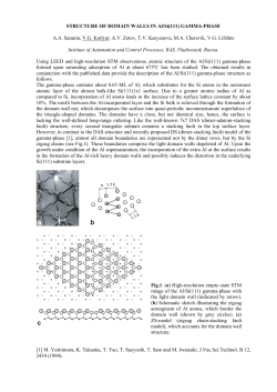
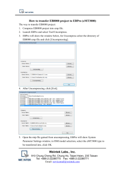


© Copyright 2026