
Journal of Science SOUTH AFRICAN
Open-access publishing in South Africa Micronutrient content of wild vegetables SOUTH AFRICAN Journal of Science South African schools need sun protection policy ISSN: 0038-2353 SEPTEMBER/OCTOBER 2014 New possibilities for research on South Africa’s shelf reef habitat volume 110 number 9/10 SEPTEMBER/OCTOBER ISSN: 0038-2353 (Print) | ISSN: 1996-7489 (Online) EDITOR-IN-CHIEF John Butler-Adam Office of the Vice Principal: Research and Graduate Education, University of Pretoria MANAGING EDITOR Linda Fick SOUTH AFRICAN Journal of Science Academy of Science of South Africa ONLINE PUBLISHING ADMINISTRATOR Nadine Wubbeling Academy of Science of South Africa volume 110 ASSOCIATE EDITORS Nicolaas Beukes number 9/10 Department of Geology, University of Johannesburg Liesbeth Botha Materials Science and Manufacturing, Council for Scientific and Industrial Research Leader Open sesame ............................................................................................................................1 Kavilan Moodley News and Views Alan Morris New possibilities for research on reef fish across the continental shelf of South Africa Anthony T.F. Bernard, Albrecht Götz, Denham Parker, Elodie R. Heyns, Sarah J. Halse, Nicholas A. Riddin, Martin K.S. Smith, Angus W. Paterson, Henning Winker, Laura Fullwood, Timothy J. Langlois & Euan S. Harvey ..................................... School of Mathematics, Statistics and Computer Science, University of KwaZulu-Natal Department of Human Biology, University of Cape Town Dan Ncayiyana Professor Emeritus, University of Cape Town Jolanda Roux Forestry and Agricultural Biotechnology Institute, University of Pretoria Pearl Sithole School of Built Environment and Development Studies, University of KwaZulu-Natal Pieter Steyn Department of Chemistry and Polymer Science, Stellenbosch University Brian van Wilgen Centre for Invasion Biology, Department of Botany and Zoology, Stellenbosch University Marco Weinberg Department of Molecular Medicine and Haematology, University of the Witwatersrand EDITORIAL ADVISORY BOARD Laura Czerniewicz 2 Book Review Excalfactoria and a bird and word book to keep you warm Duncan Mitchell ........................................................................................................................7 Interdisciplinary mentoring in science Brenda Wingfield ...................................................................................................................... 8 Commentary Good news from the South: Biodiversity mainstreaming – A paradigm shift in conservation? Brian J. Huntley ........................................................................................................................ 9 Towards SunSmart school policies in South Africa Caradee Y. Wright, Anthony J. Mundackal, Maria A. Oosthuizen & Patricia N. Albers ................................................................................... 13 Research Article Research governance and scientific knowledge production in The Gambia Frederick U. Ozor ......................................................................................................................17 Characterisation of Mycosphaerella species associated with pink spot on guava in South Africa Adriaana Jacobs, Mariette Truter & Maritha H. Schoeman .......................................................... 26 Escherichia coli with virulence factors and multidrug resistance in the Plankenburg River Corne Lamprecht, Marco Romanis, Nicola Huisamen, Anneri Carinus, Nika Schoeman, Gunnar O. Sigge & Trevor J. Britz ............................................ 32 Centre for Higher Education Development, University of Cape Town Novel CYP2E1 haplotype identified in a South African cohort Laura J. Heathfield, Shareefa Dalvie, Kusha Kalideen, Collet Dandara ........................................ 38 Roseanne Diab IziNambuzane: IsiZulu names for insects Jessica J. Cockburn, Ben Khumalo-Seegelken & Martin H. Villet ............................................... 43 Academy of Science of South Africa Christopher McQuaid Prescription patterns of enzyme-containing products in South Africa over a 2-year period Ilse Truter .................................................................................................................................. 56 Johann Mouton Advances towards the development of a cloud-resolving model in South Africa Mary-Jane M. Bopape, Francois A. Engelbrecht, David A. Randall & Willem A. Landman ..................................................................................... 61 Department of Zoology and Entomology, Rhodes University Centre for Research on Science and Technology, Stellenbosch University Maano Ramutsindela Department of Environmental & Geographical Science, University of Cape Town Published by the Academy of Science of South Africa (www.assaf.org.za) with financial assistance from the Department of Science & Technology. Design and layout SUN MeDIA Bloemfontein T: 051 444 2552 E: [email protected] Correspondence and enquiries [email protected] Copyright All articles are published under a Creative Commons Attribution Licence. Copyright is retained by the authors. Disclaimer The publisher and editors accept no responsibility for statements made by the authors. Submissions Submissions should be made at http://mc.manuscriptcentral.com/ sajs Subscriptions Subscription information can be found at www.sajs.co.za Trace element composition of two wild vegetables in response to soil-applied micronutrients Sydney Mavengahama, Willem P. de Clercq & Milla McLachlan ................................................. 73 Long bone cross-sectional geometric properties of Later Stone Age foragers and herder–foragers Michelle E. Cameron & Susan Pfeiffer ....................................................................................... 78 Tufa stromatolite ecosystems on the South African south coast Renzo Perissinotto, Tommy G. Bornman, Paul-Pierre Steyn, Nelson A.F. Miranda, Rosemary A. Dorrington, Gwynneth F. Matcher, Nadine Strydom & Nasreen Peer ............................................................................................... 89 Open access in South Africa: A case study and reflections Laura Czerniewicz & Sarah Goodier ........................................................................................... 97 Leader Open sesame The 1973 edition of the Shorter Oxford English Dictionary on Historical Principles (just 2762 pages long), which stands on a bookshelf behind my desk, has a declaration which, in the age of almost free online dictionaries and Creative Commons licences, may seem strange: The Budapest Declaration was followed by the Bethesda Statement on Open Access Publishing in June 20034 and the Berlin Declaration on Open Access to Knowledge in the Sciences and Humanities in October 2003. Since then, the movement has made considerable progress across publications, scholarly societies and nations, and the theoretical underpinnings of the need for open access have been clearly spelled out. Jean-Claude Guedon has explained the manner in which scientific cores and peripheries are created using geo-economic theory, while Erin McKiernan, a researcher working in experimental and theoretical neuroscience, points out that: All rights reserved. No part of this publication may be reproduced, stored in a retrieval system, or transmitted, in any form or by any means, electronic, mechanical, photocopying, recording, or otherwise, without the prior permission of the Oxford University Press. Presumably, this requirement applies equally to the passage just quoted as it would, for example, to citing the definition of ‘open’ as being: Every day we make amazing discoveries, some of which could even save lives. Then we lock that information in journals that most of the population cannot read. In many parts of the world, access to subscription journals is just too expensive. ….A lack of access to information hinders learning, stifles innovation and slows scientific progress.5 Open a. (adv.) 1. Of a door, gate, etc.: Not ‘put to’ not closed or shut; ‘-up’, set up so as to allow free passage through. If so, reproducing a statement does not only require an appropriate citation to the source of the information but also, more stringently, it requires permission (presumably in writing) from the Oxford University Press. Thus two copyright infringements have just occurred. There are also more radical and, at the same time, very human positions on the importance of open access. Delivering an address entitled ‘The case against privatising knowledge’, during a Vice Chancellor’s Open Lecture at the University of Cape Town last month, Dr Rajesh Tandon, who holds the UNESCO Chair in Health Research and Social Responsibility at the University, observed that Anyone who has access to the full, constantly updated, Oxford English Dictionary online faces no such restrictions, although, of course, the online version is hardly ‘set up so as to allow free passage’ unless, of course, one pays handsomely in advance. But things have changed. In 1974, I paid dearly earned postgraduate stipend funds for the Shorter Oxford English Dictionary, but still had to face the ‘rights reserved’ condition. Now one may pay and quote. The world of scholarly publishing has come a long way over the past 40 years. …knowledge industries have workers and elites…so you have the propertied classes and the property-less masses when it comes to knowledge as a commodity. It creates the divide of the haves and the have-nots, and it creates therefore control over knowledge in ways that [create] not just power…but also wealth.6 From 20 October to 26 October, the world will celebrate, and advance the cause of, open access through ‘Open Access Week,’ an event whose location is, appropriately, posted on the Scholarly Publishing and Academic Resources Commission (SPARC) site as being ‘everywhere’. SPARC Yet, despite the unquestionable logic and morality of Tandon’s observations and the valuable contributions made by McKiernan and by Guerdon, there is much progress to be made. Large publishing corporations make substantial profits by charging either articleprocessing charges or subscription fees (or both). Universities have to reduce serial subscriptions in order to cover these costs. And researchers face the damaging consequences of the remaining challenges that limit scholarly communication. I urge you to read Czernewizc and Goodier’s article in this issue for more on the topic of open access. …believes that faster and wider sharing of the outputs of the scholarly research process increases the impact of research, fuels the advancement of knowledge, and increases the return on research investments. SPARC focuses on taking action in collaboration with stakeholders – including authors, publishers, and libraries – to build on the unprecedented opportunities created by the networked digital environment to advance the conduct of scholarship.1 Here’s to Open Access Week. References As a notion, movement and, now, a well-established practice (in some quarters), open access began its freedom march with the Budapest Declaration 12 years ago.2 This declaration opens with these words: 1. SPARC. About us [homepage on the Internet]. No date [cited 2014 Sep 10]. Available from: http://www.sparc.arl.org/about 2. Digital Scholarship. Open access statements [homepage on the Internet]. No date [cited 2014 Sep 10]. Available from: http://www.digital-scholarship.org/ oab/2statements.htm An old tradition and a new technology have converged to make possible an unprecedented public good. The old tradition is the willingness of scientists and scholars to publish the fruits of their research in scholarly journals without payment, for the sake of inquiry and knowledge. The new technology is the internet. The public good they make possible is the world-wide electronic distribution of the peerreviewed journal literature and completely free and unrestricted access to it by all scientists, scholars, teachers, students, and other curious minds.3 3. Chan L, Cuplinskas D, Eisen M, Friend F, Genova Y, Guédon J-C, et al. Budapest Open Access Initiative [homepage on the Internet]. c2002 [cited 2014 Sep 10]. Available from: http://www.budapestopenaccessinitiative.org/read 4. Brown PO, Cabell D, Chakravarti A, Cohen B, Delamothe T, Eisen M, et al. Bethesda Statement on Open Access Publishing [homepage on the Internet]. c2003 [cited 2014 Sep 10]. Available from: http://www.earlham. edu/~peters/fos/bethesda.htm 5. McKiernan E. University research: If you believe in openness, stand up for it [homepage on the Internet]. c2014 [cited 2014 Sep 10]. Available from: http://www.theguardian.com/higher-education-network/blog/2014/aug/22/ university-research-publish-open-access-journal Leaders of the movement that brought the declaration to life include Jean-Claude Guedon of the University of Montreal and Lars Bjornhauge (both of whom recently addressed the South African National Scholarly Editors’ Forum in Cape Town), along with a distinguished list of people from institutions including The Wellcome and Open Society Foundations; Harvard, Minho and Southampton Universities; the Max Planck Institute and the European Union. 6. Omar Y. The case against privatising knowledge [homepage on the Internet]. c2014 [cited 2014 Sep 10]. Available from: http://www.uct.ac.za/ dailynews/?id=8800 HOW TO CITE:Butler-Adam J. Open sesame. S Afr J Sci. 2014;110(9/10), Art. #a0082, 1 page. http://dx.doi.org/10.1590/sajs.2014/a0082 © 2014. The Authors. Published under a Creative Commons Attribution Licence. South African Journal of Science http://www.sajs.co.za 1 Volume 110 | Number 9/10 September/October 2014 News & Views Page 1 of 5 AUTHORS: Anthony T.F. Bernard1,2 Albrecht Götz2,3,4 Denham Parker2,4 Elodie R. Heyns1,5 Sarah J. Halse2,4 Nicholas A. Riddin2 Martin K.S. Smith6 Angus W. Paterson5 Henning Winker7,8 Laura Fullwood9 Timothy J. Langlois10 Euan S. Harvey9 AFFILIATIONS: Department of Zoology and Entomology, Rhodes University, Grahamstown, South Africa 1 Elwandle Node, South African Environmental Observation Network, Grahamstown, South Africa 2 Development of remote stereo-video platforms New possibilities for research on reef fish across the continental shelf of South Africa Subtidal research presents numerous challenges that restrict the ability to answer fundamental ecological questions related to reef systems. These challenges are closely associated with traditional monitoring methods and include depth restrictions (e.g. safe diving depths for underwater visual census), habitat destruction (e.g. trawling), mortality of target species (e.g. controlled angling and fish traps), and high operating costs (e.g. remotely operated vehicles and large research vessels).1 Whereas many of these challenges do not apply or are avoidable in the shallow subtidal environment, the difficulties grow as one attempts to sample deeper benthic habitats. This situation has resulted in a paucity of knowledge on the structure and ecology of deep water reef habitats around the coast of South Africa2,3, and in most marine areas around the world4,5. Furthermore, the inability to effectively survey deep water benthic environments has limited the capacity of researchers to investigate connectivity between shallow and deep water habitats in a standardised and comparable fashion.6 With the recent advent of sophisticated and cost-effective remote sampling methods suitable for deep water research,1 ecologists have been able to describe finer-scale patterns of reef ecosystems in both deep and shallow waters. This ability has led to the identification of ecological drivers of shallow and deep water fish community structure in a standardised and comparable manner.7-16 The baited remote underwater stereo-video system (stereo-BRUVs; Figure 1) has been at the forefront of these developments17-19, and has emerged as the most comprehensive, precise and cost-effective tool to measure the ecosystem effects of fisheries14,20, and patterns in fish abundance7,8,15,21. a b Department of Zoology, Nelson Mandela Metropolitan University, Port Elizabeth, South Africa 3 Department of Ichthyology and Fisheries Science, Rhodes University, Grahamstown, South Africa 4 South African Institute for Aquatic Biodiversity, Grahamstown, South Africa 5 South African National Parks, Rondevlei Scientific Services, Sedgefield, South Africa 6 South African National Biodiversity Institute, Kirstenbosch Research Centre, Cape Town, South Africa 7 Centre for Statistics in Ecology, Environment and Conservation (SEEC), Department of Statistical Sciences, University of Cape Town, Cape Town, South Africa 8 Department of Environment and Agriculture, Curtin University, Perth, Australia 9 The UWA Oceans Institute and School of Plant Biology, Faculty of Natural and Agricultural Sciences, The University of Western Australia, Perth, Australia 10 Figure 1: (a) Schematic of a baited remote underwater stereo-video system (stereo-BRUVs) showing stainless steel frame (A) with pins to mount additional weights (B) and rigid centre bar (C) that holds the housed digital high-definition cameras (D). Extending perpendicularly from the centre bar is a pole that holds the synchronising diode (E) and the bait container (F). The system is linked to the surface by a buoy and rope system that attaches to the stainless steel frame (G). (b) Stereo-BRUVs deployed at a depth of 20 m on Rheeders Reef off Storms River, Tsitsikamma National Park Marine Protected Area (photo: Steve Benjamin). For the first time in South Africa, through a collaborative project of the Elwandle Node of the South African Environmental Observation Network (SAEON), the South African Institute for Aquatic Biodiversity (SAIAB), Rhodes University, the University of Western Australia, and Curtin University (Australia), stereo-BRUVs research on reef fish assemblages is being conducted within the Agulhas Ecoregion from the shallow subtidal area to the edge of the continental shelf. The purpose of this piece is to place in context the necessity of standardised research on the populations of reef fish across the continental shelf of South Africa, to put forward the case for employing stereo-BRUVs in this research, and to introduce the South African marine science community to the research possibilities available with stereo-camera systems. Video sampling techniques Although there is some variation in how different studies have approached video sampling,22-27 the techniques can broadly be grouped as (1) unbaited remote underwater video systems (RUVs), (2) baited RUVs (BRUVs), (3) diveroperated video systems (DOVs), (4) stereo-RUVs, (5) stereo-BRUVs and (6) stereo-DOVs. In addition, remotely CORRESPONDENCE TO: Anthony Bernard EMAIL: [email protected] POSTAL ADDRESS: Department of Zoology and Entomology, Rhodes University, PO Box 94, Grahamstown 6140, South Africa South African Journal of Science http://www.sajs.co.za KEYWORDS: subtidal reef fish; standardised monitoring; stereo-BRUVs; underwater video techniques HOW TO CITE: Bernard ATF, Götz A, Parker D, Heyns ER, Halse SJ, Riddin NA, et al. New possibilities for research on reef fish across the continental shelf of South Africa. S Afr J Sci. 2014;110(9/10), Art. #a0079, 5 pages. http://dx.doi.org/10.1590/sajs.2014/ a0079 © 2014. The Authors. Published under a Creative Commons Attribution Licence. 2 Volume 110 | Number 9/10 September/October 2014 News & Views Page 2 of 5 Development of remote stereo-video platforms operated vehicles (ROVs) and autonomous underwater vehicles (AUVs) equipped with video cameras are being used more frequently for research. However, both ROVs and AUVs are expensive and logistically complicated to operate and have been largely restricted to oceanographic (AUVs) or exploratory (ROVs) research. Both RUVs and BRUVs are deployed from a research vessel with the system resting on the sea floor or in the water column, while tethered to a surface marker buoy or to the research vessel. The only distinction between these two approaches is that BRUVs use a food-based attractant to draw fish into the field of view of the camera. DOV is synonymous with underwater visual census (UVC), except that the survey is recorded and the researcher identifies and counts fish post sampling from the video footage, as opposed to identifying and counting the fish while underwater (as in UVC). Stereovideo sampling is a variation of mono-video camera techniques (RUVs, BRUVs and DOVs) that allow for fish lengths to be measured and the survey area to be quantified, greatly increasing the data output per sample and the value of the data for studying the effects of fishing.14 targeted by fisheries and accurate information on the size structure of these populations.14,18,19,24,30,36 Remote video sampling techniques are flexible in that the systems can be deployed with or without bait, or with the bait type varying between units or deployments, and can be tailored to address a multitude of questions by targeting specific components of the fish community. As such, remote video sampling techniques reduce the research footprint and provide data capable of addressing research and management questions across geographical and depth gradients, within special management areas (e.g. no-take marine protected areas, MPAs) and across different habitats. Importantly, the feasibility of long-term standardised monitoring will be increased significantly by the cost-efficiency of the method. Since the mid-1990s there has been an exponential increase in the number of research articles published in peer-reviewed scientific journals that employed BRUVs, RUVs, DOVs or their stereo-video equivalents to collect fish assemblage data from subtidal reefs across continental shelves (Figure 2). Stereo-video sampling techniques first emerged in the early 1980s28; however, it was only in the mid-1990s that development of the remote stereo-video approach was initiated by researchers at Otago University and Melbourne University.24 Only in the last 4 years has the method expanded globally, resulting in a rapid increase in the number of publications based on data collected with this approach (Figure 2). Further growth in the publication rate can be expected over the next few years as the tools become more available and awareness of the new research possibilities they provide increases. One of the major advantages of stereo-video over mono-video techniques is that it allows for precise length measurement of fish underwater. This advantage means that the potential for observer error is avoided (compared with UVC) and the need to remove fish from the water, which frequently leads to barotrauma, is eliminated (compared with controlled angling and fish traps).17,37,38 The size distribution of a fish community is a more sensitive measure of fishing pressure than abundance, as larger individuals of a species are typically more aggressive and caught first when fishing.1 Research from Western Australia has demonstrated that the size data collected with stereo-BRUVs are comparable to fisheries-dependent data sources and are therefore potentially useful for informing management of stocks.36,39 In addition, size-based indicators, such as mean length in a population or community, mean maximum length in a community, and the slope and intercept of size spectra, are particularly useful for long-term ecosystem-based fisheries management (EBFM).40,41 Furthermore, the use of stereo-video also allows the distance from the cameras to a fish to be measured and hence the area sampled can be standardised.42 Several studies have compared the benefits and shortcomings of different underwater video sampling techniques,19,29-31 or contrasted them with more established subtidal sampling techniques such as UVC18,32,33, controlled angling14,34, research trawling25,35 or trapping35,36. In general, results show that the stereo-BRUVs technique outperforms all other available methods with the data characterised by low levels of variability, high levels of species richness, high abundances of species Over the last 4 years, single camera remote underwater video systems (RUVs and BRUVs) have been successfully employed to survey the reef fish communities in the Tsitsikamma National Park, Still Bay National Park and Table Mountain National Park MPAs in South Africa.31,43,44 The results suggest that BRUVs are highly suitable for obtaining relative abundance data for most of the reef fish species occurring in the Agulhas Ecoregion. Furthermore, data collected in the Tsitsikamma National Park a 30 b 16 14 25 10 15 8 6 10 4 5 2 0 2012 2012 2010 2008 2006 2004 2002 2000 1998 1994 2010 2000 1990 1980 1970 1960 1950 0 1996 Number of publications 12 20 Year Figure 2: Number of articles published in peer-reviewed scientific journals (a) from 1952 to June 2013 that included use of video sampling techniques and (b) from 1994 that included use of stereo-video sampling techniques. The bars indicate the number of articles published by July 2013, while the open circle indicates the expected number of published articles by the end of 2013. The articles were collated by means of academic publication search engines (Academic Search Premier, Cambridge Journals, CSIRO, ESA, JSTOR, Google Scholar, Inter-Research, Science Direct, Sci-Verse Scopus, Springer Link, Web of Knowledge) and reference list reviews of key literature. Search terms entered included: BRUVs, RUVs, DOVs, remote video and fish. Studies using remotely operated vehicles and autonomous underwater vehicles and those with data collected beyond the continental shelves were excluded. South African Journal of Science http://www.sajs.co.za 3 Volume 110 | Number 9/10 September/October 2014 News & Views Page 3 of 5 Development of remote stereo-video platforms across these broad distributional ranges in a standardised and comparable fashion is required to provide data that promotes effective management of such species. The remote underwater stereo-video system, whether baited or unbaited, offers an opportunity to meet this need. MPA, using six different techniques, show that BRUVs detected 92% of all bony fish and 71% of all cartilaginous species recorded by the six methods, compared with 68% and 43%, respectively, for the second best method – RUVs (Table 1).45 Interestingly, in the same study UVC recorded zero cartilaginous species and only 60% of the bony fish species, even though it had three times the sampling effort compared with both RUVs and BRUVs.45 These results further emphasised the efficiency of BRUVs, with the method requiring only 21 samples per annum to detect a 10% increase in the abundance of important commercial fisheries species, compared with 49 samples required by RUVs and 72 samples required by UVC.45 Conclusions There is a growing global recognition that high-resolution, nondestructive and in-situ stereo-video techniques can provide improved understanding of fine-scale ecology on deep and shallow reef habitats, and deliver data that support effective EBFM. Preliminary work in South Africa has proved that the method can be cost-efficiently employed by small research teams working off small vessels. The stereo-video research platform developed at SAIAB and SAEON will be able to operate down to depths of 250 m, covering the entire depth range of the continental shelf of South Africa, and will open an extensive array of new research possibilities to scientists based at tertiary education facilities and research institutes in South Africa. The next step is to implement priority research projects that, for example, provide data necessary to develop an understanding of the ecology of shallow- and deep-water habitats and their connectivity, and to determine the spatial patterns of abundance and biomass distributions of vulnerable and endemic fish species. This will support the implementation of effective EBFM and form the basis of long-term monitoring programmes that inform adaptive EBFM. During 2013, stereo-BRUVs were deployed for the first time in South Africa (and Africa), to collect fish assemblage data within the Tsitsikamma National Park MPA. A total of 194 samples, equating to 388 h of video footage, was collected from inside and outside the MPA using four units during 17 sampling days. Sampling depth ranged from 6 m to 80 m, encompassing the deepest extent of the reef habitat inside the MPA and equivalent habitat outside the MPA. All sampling was conducted off an 8-m semi-rigid ski-boat fitted with a simple capstan winch to retrieve the weighted systems. Preliminary analysis of 36 samples has resulted in the detection of 41 species and a total of 3644 size measurements, showing that the stereo-BRUVs not only provide the same benefits as the mono-camera BRUVs, but also produce a considerable amount of length frequency data (±100/sample). Importance of standardised monitoring Beyond the scientific value, hours of video footage will be available for educational purposes to raise awareness regarding the vulnerability of reef fishes and the role of no-take MPAs in protecting reef ecosystems. This material can be used to stimulate interest in marine biology amongst the younger generation and inform communities on the importance of MPAs and fisheries regulations. Over the last few decades it has become evident that both management and monitoring of fish resources have been inadequate, or inappropriate, to ensure the conservation of biodiversity and sustainable utilisation of target species.46-49 The single or multi-species approach to traditional management is considered by many to be outdated, particularly for reef fish, and there is a drive to implement holistic EBFM.3,47,48,50 Similarly, the assumption that managers can rely on resource users to abide by regulations has been repeatedly disproved, compelling managers to adopt approaches that are feasible to manage and enforce, such as notake MPAs.3,48,49 Acknowledgements Funding was provided by the South African Institute for Aquatic Biodiversity, the South African Environmental Observation Network, the British Ecological Society, the Western Indian Ocean Marine Science Association and the National Research Foundation of South Africa. Ecosystem-based fisheries management requires sound knowledge on the ecology of the natural systems being managed.50,51 Because of the vulnerable nature of populations of over-exploited fish species, monitoring methods need to be non-destructive to remove the possibility of additional impacts on stocks. Furthermore, many reef fish species occupy broad depth ranges during the course of their life histories.52-54 In South Africa, this applies for most of the important endemic reef dwelling species targeted in the line-fishery industry, with some occupying a depth range in excess of 150 m.52,53 This is true for species such as carpenter (Argyrozona argyrozona), dageraad (Chrysoblephus cristiceps), red stumpnose (C. gibbiceps), roman (C. laticeps), black musselcracker (Cymatoceps nasutus), blue hottentot (Pachymetopon aeneum), hottentot seabream (Pachymetopon blochii), red steenbras (Petrus rupestris), scotsman (Polysteganus praeorbitalis) and panga (Pterogymnus laniarius), many of which are considered over-exploited and are listed by the South African Sustainable Seafood Initiative as species of concern or as unsustainable.48,49,55 Adequate monitoring Table 1: References 1. Murphy HM, Jenkins GP. Observational methods used in marine spatial monitoring of fishes and associated habitats: A review. Mar Freshwater Res. 2010;61:236–252. http://dx.doi.org/10.1071/MF09068 2. Griffiths CL, Robinson TB, Lange L, Mead A. Marine biodiversity in South Africa: An evaluation of current states of knowledge. PLoS ONE. 2010;5:e12008. http://dx.doi.org/10.1371/journal.pone.0012008 3. Sink KJ, Attwood CG, Lombard AT, Grantham H, Leslie R, Samaai T, et al. Spatial planning to identify focus areas for offshore biodiversity protection in South Africa. Final report for the Offshore Marine Protected Area Project. Cape Town: South African National Biodiversity Institute; 2011. 4. Miller K, Neil H, Tracey D. Recent advances in deep-sea coral science and emerging links to conservation and management of deep-sea ecosystems. Mar Ecol Prog Ser. 2009;397:1–5. http://dx.doi.org/10.3354/meps08452 Fish species sampled by means of controlled angling (CA), fish trap (FT), remotely operated vehicle (ROV), remote underwater video systems (RUVs), baited RUVs (BRUVs) and underwater visual census (UVC) in the Tsitsikamma National Park Marine Protected Area during a simultaneous method comparison.45 Each method was allocated two randomly selected days for data collection within a 24-day sampling period. Method (number of samples) Common name (total number of species recorded with all six methods) CA (16) Jawless fishes (1 species) FT (25) ROV (7) RUVs (10) BRUVs (10) UVC (30) 1 Cartilaginous fishes (7 species) 3 4 1 3 5 0 Bony fishes (25 species) 11 5 9 17 23 15 South African Journal of Science http://www.sajs.co.za 4 Volume 110 | Number 9/10 September/October 2014 News & Views Page 4 of 5 Development of remote stereo-video platforms 5. Quattrini AM, Ross SW, Carlson MCT, Nizinski MS. Megafaunal-habitat associations at a deep-sea coral mound off North Carolina, USA. Mar Biol. 2012;159:1079–1094. 23. Willis TJ, Babcock RC. A baited underwater video system for the determination of relative density of carnivorous reef fish. Mar Freshwater Res. 2000;51:755–763. http://dx.doi.org/10.1071/MF00010 6. Levin LA, Dayton PK. Ecological theory and continental margins: Where shallow meets deep. Trends Ecol Evol. 2009;1142:606–617. http://dx.doi. org/10.1016/j.tree.2009.04.012 24. Harvey ES, Fletcher D, Shortis M. Estimation of reef fish length by divers and by stereo-video: A first comparison of the accuracy and precision in the field on living fish under operational conditions. Fish Res. 2002;57:255–265. http://dx.doi.org/10.1016/S0165-7836(01)00356-3 7. Moore CH, Harvey ES, Van Niel KP. Spatial prediction of demersal fish distributions: Enhancing our understanding of species-environment relationships. ICES J Mar Sci. 2009;66:2068–2075. http://dx.doi. org/10.1093/icesjms/fsp205 25. Cappo M, Speare P, De’ath G. Comparison of baited remote underwater video stations (BRUVS) and prawn (shrimp) trawls for assessments of fish biodiversity in inter-reefal areas of the Great Barrier Reef Marine Park. J Exp Mar Biol Ecol. 2004;302:123–152. http://dx.doi.org/10.1016/j. jembe.2003.10.006 8. Moore CH, Harvey ES, Niel K. The application of predicted habitat models to investigate the spatial ecology of demersal fish assemblages. Mar Biol. 2010;157:2717–2729. http://dx.doi.org/10.1007/s00227-010-1531-4 26. Pelletier D, Leleu K, Mallet D, Mou-Tham G, Hervé G, Boureau M, et al. Remote high-definition rotating video enables fast spatial survey of marine underwater macrofauna and habitats. PLoS ONE. 2012;7:e30536. http:// dx.doi.org/10.1371/journal.pone.0030536 9. Moore CH, Van Niel K, Harvey ES. The effect of landscape composition and configuration on the spatial distribution of temperate demersal fish. Ecography. 2011;34:425–435. http://dx.doi.org/10.1111/j.1600-0587.2010.06436.x 27. Santana-Garcon J, Leis JM, Newman SJ, Harvey ES. Presettlement schooling behaviour of a priacanthid, the Purplespotted Bigeye Priacanthus tayenus (Priacanthidae: Teleostei). Environ Biol Fishes. 2013;97:277–283. http:// dx.doi.org/10.1007/s10641-013-0150-6 10. Watson DL, Anderson MJ, Kendrick GA, Nardi K, Harvey ES. Effects of protection from fishing on the lengths of targeted and non-targeted fish species at the Houtman Abrolhos Islands, Western Australia. Mar Ecol Prog Ser. 2009;384:241–249. http://dx.doi.org/10.3354/meps08009 28. Dill LM, Dunbrack RL, Major PF. A new stereophotographic technique for analyzing the three-dimensional structure of fish schools. Environ Biol Fishes. 1981;6:7–13. http://dx.doi.org/10.1007/BF00001793 11. Malcolm H, Jordan A, Smith SD. Testing a depth-based habitat classification system against reef fish assemblage patterns in a subtropical marine park. Aquat Conserv Mar Freshwater Ecosyst. 2011;21:173–185. http://dx.doi. org/10.1002/aqc.1165 29. Harvey ES, Cappo M, Butler JJ, Hall N, Kendrick GA. Bait attraction affects the performance of remote underwater video stations in assessment of demersal fish community structure. Mar Ecol Prog Ser. 2007;350:245–254. http:// dx.doi.org/10.3354/meps07192 12. Mcilwain JL, Harvey ES, Grove S, Shiell G, Al Oufi H, Al Jardani N. Seasonal changes in a deep-water fish assemblage in response to monsoongenerated upwelling events. Fish Oceanogr. 2011;20:497–516. http://dx.doi. org/10.1111/j.1365-2419.2011.00598.x 30. Watson DL, Harvey ES, Fitzpatrick BM, Langlois TJ, Shedrawi G. Assessing reef fish assemblage structure: How do different stereo-video techniques compare? Mar Biol. 2010;157:1237–1250. http://dx.doi.org/10.1007/ s00227-010-1404-x 13. Harvey ES, Dorman SR, Fitzpatrick C, Newman SJ, McLean DL. Response of diurnal and nocturnal coral reef fish to protection from fishing: an assessment using baited remote underwater video. Coral Reefs. 2012;31:939–950. http:// dx.doi.org/10.1007/s00338-012-0955-3 31. Bernard ATF, Götz A. Bait increases the precision in count data from remote underwater video for most subtidal reef fish in the warm-temperate Agulhas bioregion. Mar Ecol Prog Ser. 2012;471:235–252. http://dx.doi.org/10.3354/ meps10039 14. Langlois TJ, Harvey ES, Meeuwig JJ. Strong direct and inconsistent indirect effects of fishing found using stereo-video: Testing indicators from fisheries closures. Ecol Indic. 2012; 23:524–534. http://dx.doi.org/10.1016/j. ecolind.2012.04.030 32. Colton MA, Swearer SE. A comparison of two survey methods: Differences between underwater visual census and baited remote underwater video. Mar Ecol Prog Ser. 2010;400:19–36. http://dx.doi.org/10.3354/meps08377 15. Langlois TJ, Radford BT, Van Niel KP, Meeuwig JJ, Pearce AF, Rousseaux CSG, et al. Consistent abundance distributions of marine fishes in an old, climatically buffered, infertile seascape. Glob Ecol Biogeogr. 2012;21:886– 897. http://dx.doi.org/10.1111/j.1466-8238.2011.00734.x 33. Pelletier D, Leleu K, Mou-Tham G, Guillemot N, Chabanet P. Comparison of visual census and high definition video transects for monitoring coral reef fish assemblages. Fish Res. 2011;107:84–93. http://dx.doi.org/10.1016/j. fishres.2010.10.011 16. Zintzen V, Anderson MJ, Roberts CD, Harvey ES, Stewart AL, Struthers CD. Diversity and composition of demersal fishes along a depth gradient assessed by baited remote underwater stereo-video. PLoS ONE. 2012;7:e48522. http:// dx.doi.org/10.1371/journal.pone.0048522 34. Willis TJ, Millar RB, Babcock RC. Detection of spatial variability in relative density of fishes: Comparison of visual census, angling and, baited underwater video. Mar Ecol Prog Ser. 2000;198:249–260. http://dx.doi. org/10.3354/meps198249 17. Harvey ES, Shortis M. A system for stereo-video measurement of sub-tidal organisms. J Mar Tech Soc. 1995;29:10–22. 35. Priede I, Bagley P, Smith A, Creasey S, Merrett N. Scavenging deep demersal fishes of the Porcupine Seabight, north-east Atlantic: Observations by baited camera, trap and trawl. J Mar Biol Assoc UK. 1994;74:481–498. http:// dx.doi.org/10.1017/S0025315400047615 18. Watson DL, Harvey ES, Anderson MJ, Kendrick GA. A comparison of temperate reef fish assemblages recorded by three underwater stereovideo techniques. Mar Biol. 2005;148:415–425. http://dx.doi.org/10.1007/ s00227-005-0090-6 36. Harvey ES, Newman SJ, McLean DL, Cappo M, Meeuwig JJ, Skepper CL. Comparison of the relative efficiencies of stereo-BRUVs and traps for sampling tropical continental shelf demersal fishes. Fish Res. 2012;125– 126:108–120. http://dx.doi.org/10.1016/j.fishres.2012.01.026 19. Langlois TJ, Harvey ES, Fitzpatrick B, Meeuwig JJ, Shedrawi G, Watson DL. Cost-efficient sampling of fish assemblages: Comparison of baited video stations and diver video transects. Aquat Biol. 2010;9:155–168. http://dx.doi. org/10.3354/ab00235 37. Shortis MR, Ravanbakskh M, Shaifat F, Harvey ES, Mian A, Seager JW, et al. A review of techniques for the identification and measurement of fish in underwater stereo-video image sequences. Proc SPIE. 2013;8791. http:// dx.doi.org/10.1117/12.2020941 20. McLean DL, Harvey ES, Meeuwig JJ. Declines in the abundance of coral trout (Plectropomus leopardus) in areas closed to fishing at the Houtman Abrolhos Islands, Western Australia. J Exp Mar Biol Ecol. 2011;406:71–78. http://dx.doi.org/10.1016/j.jembe.2011.06.009 38. Kerwath SE, Wilke CG, Götz A. The effects of barotrauma on five South African line caught fishes. Afr J Mar Sci. 2013;35:243–252. http://dx.doi.org /10.2989/1814232X.2013.805594 21. Fitzpatrick BM, Harvey ES, Heyward AJ, Twiggs EJ, Colquhoun J. Habitat specialization in tropical continental shelf demersal fish assemblages. PLoS ONE. 2012;7:e39634. http://dx.doi.org/10.1371/journal.pone.0039634 39. Langlois TJ, Fitzpatric BR, Fairclough DV, Wakefield CB, Hesp SA, McLean DL, et al. Similarities between line fishing and baited stereo-video estimations of length-frequency. Novel application of kernel density estimates. PLoS ONE. 2012;7(11):e45973. http://dx.doi.org/10.1371/journal.pone.0045973 22. Francour P, Liret C, Harvey ES. Comparison of fish abundance estimates made by remote underwater video and visual census. Naturalista Siciliana. 1999;XXIII(suppl):155–168. South African Journal of Science http://www.sajs.co.za 5 Volume 110 | Number 9/10 September/October 2014 News & Views Page 5 of 5 Development of remote stereo-video platforms 40. Shin Y, Rochet M, Jennings S, Field J, Gislason H. Using size-based indicators to evaluate the ecosystem effects of fishing. ICES J Mar Sci. 2005;62:384– 396. http://dx.doi.org/10.1016/j.icesjms.2005.01.004 48. Sink KJ, Holness S, Harris L, Majiedt P, Atkinson L, Robinson T, et al. National biodiversity assessment 2011: Technical report: Volume 4: Marine and Coastal Component. Pretoria: South African National Biodiversity Institute; 2012. 41. Trebilco R, Baum JK, Salomon AK, Dulvy NK. Ecosystem ecology: Size-based constraints on the pyramids of life. Trends Ecol Evol. 2013;28:423–431. http://dx.doi.org/10.1016/j.tree.2013.03.008 49. Department of Agriculture, Forestry and Fisheries (DAFF). Status of the South African marine fishery resources. Cape Town: Chief Directorate Fisheries Research, Fisheries Branch; 2012. 42. Harvey ES, Fletcher D, Shortis MR, Kendrick GA. A comparison of underwater visual distance estimates made by SCUBA divers and a stereo-video system: Implications for underwater visual census of reef fish abundance. Mar Freshwater Res. 2004;55:573–580. http://dx.doi.org/10.1071/MF03130 50. Johnson AF, Jenkins SR, Hiddink JG, Hinz H. Linking temperate demersal fish species to habitat: Scales, patterns and future directions. Fish Fish. 2012;14:256–280. http://dx.doi.org/10.1111/j.1467-2979.2012.00466.x 43. De Vos L, Götz A, Winker H, Attwood CG. Optimal BRUVs (baited remote underwater video system) survey design for reef fish monitoring in the Stilbaai Marine Protected Area. Afr J Mar Sci. 2014;36:1–10. http://dx.doi.or g/10.2989/1814232X.2013.873739 51. Fletcher WJ, Shaw J, Metcalf SJ, Gaughan DJ. An ecosystem based fisheries management framework: The efficient, regional-level planning tool for management agencies. Mar Policy. 2010;34:1226–1238. http://dx.doi. org/10.1016/j.marpol.2010.04.007 44. Sanguinetti C. Patterns in reef fish assemblages as determined by baited remote underwater video (BRUV) along the western side of False Bay: effects of site, depth, and protection [MSc thesis]. Cape Town: University of Cape Town; 2013. 52. Mann BQ. South African marine linefish status reports. Oceanographic Research Institute Special Publication 7. Durban: South African Association for Marine Biological Research; 2000. 45. Bernard ATF. Towards a cost-efficient & standardised monitoring protocol for subtidal reef fish in the Agulhas Ecoregion of South Africa [PhD thesis]. Grahamstown: Rhodes University; 2012. 53. Mann BQ. South African marine linefish species profiles. Oceanographic Research Institute Special Publication 9. Durban: South African Association for Marine Biological Research; 2013. 46. Gray JS. Marine biodiversity: Patterns, threats and conservation needs. Biodivers Conserv. 1997;6:153–175. http://dx.doi.org/10.1023/A:1018335901847 54. Collins A, McBride R. Demographics by depth: Spatially explicit life-history dynamics of a protogynous reef fish. Fish Bull. 2011;109:232–242. 47. Pikitich EK, Santora C, Babcock EA, Bakun A, Bonfil R, Conover DO, et al. Ecosystem-based fishery management. Science. 2004;305:346–347. http:// dx.doi.org/10.1126/science.1098222 55. South African Sustainable Seafood Initiative (SASSI). Consumer seafood pocket guide [document on the Internet]. c2013 [cited 2013 July 01]. Available from: http://www.wwfsassi.co.za/pocketguide.pdf. South African Journal of Science http://www.sajs.co.za 6 Volume 110 | Number 9/10 September/October 2014 Book Review Page 1 of 1 BOOK TITLE: Latin for birdwatchers BOOK COVER: AUTHORS: Roger Lederer and Carol Burr ISBN: 9781775840930 PUBLISHER: Struik Nature, Cape Town, ZAR220 PUBLISHED: 2014 REVIEW TITLE: Excalfactoria and a bird and word book to keep you warm REVIEWER: Duncan Mitchell1,2 EMAIL: [email protected] AFFILIATIONS: Rand Barbets Bird Club of BirdLife South Africa, Johannesburg, South Africa 1 Emeritus Professor, School of Physiology, University of the Witwatersrand, Johannesburg, South Africa 2 POSTAL ADDRESS: Brain Function Research Group, School of Physiology, Faculty of Health Sciences, University of the Witwatersrand, Private Bag 3, Wits 2050, South Africa HOW TO CITE: Mitchell D. Excalfactoria and a bird and word book to keep you warm. S Afr J Sci. 2014;110(9/10), Art. #a0077, 1 page. http://dx.doi. org/10.1590/sajs.2014/a0077 © 2014. The Authors. Published under a Creative Commons Attribution Licence. South African Journal of Science http://www.sajs.co.za Excalfactoria and a bird and word book to keep you warm Excalfactoria and a bird and word book to keep you warm Chico, California, bordered by almond orchards and home to the US Yo-Yo Museum, seems an unlikely place to find an erudite husband-and-wife team who love birds, and words, and Latin. Roger Lederer and Carol Burr both have PhDs and both are Emeritus Professors at California State University, Chico – he of Biological Sciences and she of English. On his website, Lederer says he ‘knows exactly what birds you will find anywhere in the world’; he has travelled to over 100 countries. He has written five previous books on birds, and a 1984 textbook on Ecology and Field Biology. Burr is using her retirement from teaching English and Women’s Studies to paint and draw, in oils, water colours, pen and coloured pencils (the medium that she has used in illustrating Latin for Birdwatchers). Latin for Birdwatchers sets out to explore and explain 3000 scientific bird names, listed alphabetically. It does not claim to be comprehensive: there are about 20 000 bird names. Those scientific names are the Linnaean binomial names, that is, the paired names of genus and species in the system set up by Carl Linnaeus (1707–1778) for naming everything alive. Although BirdLife South Africa works hard to promote the use of these names, birdwatchers tend to show less interest in Linnaean binomials than do, for example, tree watchers, but they are the only definitive names for birds (and trees). Most Linnaean binomials for birds are Latin-derived constructs, but enough, and especially those for African bird species, are Greek-derived to have justified ‘and Greek’ in the book’s title: meleagris, as in Numida meleagris (helmeted guineafowl) is the Greek word for guinea fowl and Tyto, as in Tyto alba (barn owl), the Greek word for owl. Some names are derived from other languages. Pitta – as in Pitta angolensis (African pitta) – is an Indian word meaning ‘little bird’. The kori in Ardeotis kori (kori bustard) comes from its Setswana name kgôri. For all the Linnaean binomials listed, the authors offer an easy-to-interpret pronunciation as if in post-Renaissance Latin, with the appropriate syllable emphasised: mel-ee-AH-gris and TI-to. Most Linnaean binomials are descriptive of the bird’s biology, and for each of those listed the authors explain the derivation. To cover 3000 names, their explanations necessarily have to be brief, although they have expanded a few in boxes that they have called ‘Latin in action’ (Picus, after whom the woodpecker family Picidae was named, was a king in Roman mythology turned into a woodpecker by the witch Circe). Wildlife author Richard Conniff, who reviewed the book, otherwise favourably, in May 2014 for the Wall Street Journal, complained that some explanations were too brief to be satisfactory. (The US version that he reviewed was called Latin for Bird Lovers; South Africans apparently are allowed to ‘watch’ birds but not to ‘love’ them.) I did not find the explanations unsatisfactorily brief; they are more comprehensive, for example, than the explanations in the ‘big Roberts’1, which, of course, admirably serves many purposes other than explaining binomials. Some Linnaean binomials are not descriptive but acknowledge a person associated with a species, and the person celebrated is identified in a phrase: Neergaard (‘recruiter for Witwatersrand mines’) of Neergaard’s sunbird Cinnyris neergaardi is recognised, as is Barlow (‘South African businessman’) of Barlow’s lark Calendulauda barlowi and Vigors (‘Irish secretary of the Zoological Society of London’) of the Karoo korhaan Eupodotis vigorsii, but not Stierling of Stierling’s wren-warbler Calamonastes stierlingi or Rüppell of Rüppell’s vulture Gyps rueppellii. Some Latin names are onomatopoeic: Pitohui as in Pitohui dichrous (hooded pitohui, a poisonous oriole-like bird from New Guinea) ‘is the sound made after a human tastes and immediately rejects the poisonous bird’, and Tockus, the hornbill genus, comes from ‘a Portuguese imitation of the bird’s call’. Here are some of the descriptive Latin names related to birds well known to South African birdwatchers: ‘cista, a wooden basket, and colo, dwell’, describing the nesting habits of cisticolas; Ispidina ‘from hispidus, rough, shaggy, hairy, as in Ispidina picta’ (African pigmy kingfisher); Mirafra in Mirafra africana (rufous-naped lark, called Mirafra mirafra in the book) from ‘miras, wonderful, and afra, African’; ‘Musophaga, from musa, banana, and phagus, eater of, as in Musophaga rossae’ (Ross’s turaco). Just the list of Linnaean binomial names would have entertained me sufficiently, but that is not where Lederer and Burr left their book. They added two-page biosketches of 11 ‘famous birders’, including John Gould (1804–1881), after whom 24 bird species have been named (more than after anyone else), and the real James Bond (1900–1989), after whom Ian Fleming named 007. There are 20 one-page ‘genus profiles’, including the Laniidae, from lanius, Latin for ‘butcher’, amongst which are the fiscals, from the Afrikaans fiskaal, meaning, according to Lederer and Burr, ‘a public official, particularly a hangman’. There are eight two-page essays on bird biology, containing interesting information that even experienced birdwatchers may not know. And then every page has one or more illustrations by Burr, attractively drawn not so much for ornithological accuracy but, as she herself said in an interview on Chico’s Northstate Public Radio, to try to capture the personality and aesthetics of the bird. The book has been produced beautifully by Quid Publishing in the UK for Struik Nature. It has a textured hard cover, is a comfortable size, and is printed on elegant fulvus paper. I found some repetition in the grammar and a few typographical errors, which easily can be fixed in later editions, and do not intrude in this edition. If you like birds and words, and especially if you like Latin and Greek, read Latin for Birdwatchers cover to cover, or explore a favourite genus or historical ornithologist, or absorb a bird’s personality from an illustration, or just take a lucky dip. I do not think that the book will work well in electronic format. This is a book that you need to hold in your hands, to keep you warm. And I’ll leave it to you to discover why the king quail is called Excalfactoria chinensis. Reference 1. Hockey PAR, Dean WRJ, Ryan PG. Roberts birds of southern Africa. 7th ed. Cape Town: The Trustees of the John Voelcker Bird Book Fund; 2005. 7 Volume 110 | Number 9/10 September/October 2014 Book Review Page 1 of 1 Interdisciplinary mentoring in science Interdisciplinary mentoring in science BOOK TITLE: Interdisciplinary mentoring in science : Strategies for success Mentorship is something I am passionate about and it was possibly for this reason that I was asked to provide a review on this book. As a starting point, I should mention that this book is not so much about mentorship as about how to put in place a mentoring programme in a scientific organisation. It is thus not a book that one should just read, but a book that one should read with the idea of putting into practice the tasks suggested. BOOK COVER: The book is interesting and challenging and I appreciated a number of aspects about it. However, as a scientist in a developing world environment I did find the strong American focus distracting at times. Perhaps this focus was to be expected but there are some strong statements about the need for mentoring in the developing world, and particularly in sub-Saharan Africa, and I would have hoped that the American view point would not be quite so overwhelming. My advice to readers is to thus try to get beyond this view as the book does provide some very useful insights which do have an international value. The first four chapters deal overwhelmingly with minority mentoring and gender diversity. All but one of the experts who are showcased in the book are women. From a South African perspective, there is a disjunction, as our socalled previously disadvantaged communities are in the majority. Perhaps the real ‘take-home message’ here is the importance of diversity. In South Africa, diversity is pretty much a given – which does not mean that we necessarily always appreciate the possible advantages of our diversity. My own opinion is that there is only one thing worse than a committee of only men: a committee of only women. AUTHOR: Ofelia A. Olivero ISBN: 9780124159624 PUBLISHER: Academic Press, Oxford, USD34.95 PUBLISHED: 2013 REVIEW TITLE: Interdisciplinary mentoring in science My favourite chapter was without question Chapter 5, which focuses on ‘Interdisciplinary Mentoring’. This chapter was for me the most important one of the book. The value of interdisciplinarity has always been obvious to me, but this chapter served to highlight some examples as well as to explain the issues in ways that I would not have thought about. In South Africa we engage with scientists from very different backgrounds, yet very little time is spent considering these backgrounds and how some of the traditional Western norms of a scientific career can be at odds with traditional expectations. This is not to say that we have to either adopt the Western norms or just accept tradition. We need to converse and find ways of doing things even better. The book gives some details about what is needed to be a good mentor and I would hope that most scientists would reflect on this section. So often the ‘lone inventor/innovator or the multifunded, independent laboratory head, is seen as the pinnacle of success’. While this can be the case, and often has been the case in the past, I think that often the nature of how we practise science today has meant that things have changed. In most disciplines we are all involved in increasingly large data sets, meaning that collaboration, particularly across many disciplines, has become the norm. Thus we all must learn how to collaborate and put in place sustainable research cultures. There is no question that mentorship will play an important role in doing so. I enjoyed reading this book and will be recommending it to others who have an interest in managing research programmes. In many ways, the book is very timely as we all are dealing with many of the issues discussed and could learn a lot more about mentorship. REVIEWER: Brenda Wingfield EMAIL: [email protected] AFFILIATION: Faculty of Natural and Agricultural Sciences, University of Pretoria, Pretoria, South Africa POSTAL ADDRESS: Faculty of Natural and Agricultural Sciences, University of Pretoria, Private Bag X20, Hatfield 0028, Pretoria HOW TO CITE: Wingfield B. Interdisciplinary mentoring in science. S Afr J Sci. 2014;110(9/10), Art. #a0081, 1 page. http://dx.doi. org/10.1590/sajs.2014/a0081 © 2014. The Authors. Published under a Creative Commons Attribution Licence. South African Journal of Science http://www.sajs.co.za 8 Volume 110 | Number 9/10 September/October 2014 Commentary Page 1 of 4 AUTHOR: Brian J. Huntley1 AFFILIATION: Centre for Invasion Biology, Stellenbosch University, Stellenbosch, South Africa 1 CORRESPONDENCE TO: Brian Huntley EMAIL: [email protected] POSTAL ADDRESS: Otter Close, Box 334, Betty’s Bay 7141, South Africa KEYWORDS: biodiversity; mainstreaming; conservation; Global Environment Facility HOW TO CITE: Huntley BJ. Good news from the South: Biodiversity mainstreaming – A paradigm shift in conservation? S Afr J Sci. 2014;110(9/10), Art. #a0080, 4 pages. http://dx.doi. org/10.1590/sajs.2014/a0080 Biodiversity mainstreaming – A paradigm shift in conservation? Good news from the South: Biodiversity mainstreaming – A paradigm shift in conservation? ‘Bad governance stifles everything’ said ecologist Richard Cowling, a pioneer in promoting mainstreaming approaches to conserving biodiversity. Cowling was addressing an international workshop convened in Cape Town in October 2013 to review progress in the impressive body of 327 projects in 135 countries supported since the late 1990s by the Global Environment Facility (GEF).1 With over USD1.6 billion invested by the GEF, and USD5.6 billion in co-financing by partners, the mainstreaming agenda is one of the largest biodiversity initiatives on record. A whopping 48% of these funds went to the 10 countries that hold most of the world’s biodiversity treasure troves – Brazil, India, China, Mexico, South Africa, Colombia, Russian Federation, Indonesia, Vietnam and Argentina. The obvious reciprocal to bad governance – good governance – certainly holds true, and is demonstrated by the success of mainstreaming projects in post-apartheid South Africa and in that icon of democratic good governance, Costa Rica.2,3 These two countries lead the world in innovative approaches to biodiversity conservation, most especially in moving from the traditional ‘protected areas’ model to an integrated landscape paradigm. The emerging trends and the challenges to the successful implementation of mainstreaming are considered here. What is ‘biodiversity mainstreaming’? Emerging as an effective and synergistic interface between conservation science and sustainable development, biodiversity mainstreaming has been variously defined over the past decade,4,5 most recently at the Cape Town workshop, at which conservation practitioners and researchers from around the globe defined it thus: Biodiversity mainstreaming is the process of embedding biodiversity considerations into policies, strategies and practices of key public and private actors that impact or rely on biodiversity, so that it is conserved and sustainably and equitably used both locally and globally. The mainstreaming approach has gained traction across major international organisations, as reflected in the strategic plans and programmes of the Convention on Biological Diversity – the United Nations Environment Programme, United Nations Development Programme and the World Bank – and, most recently, the G20’s post2015 sustainable development agenda.6,7 Mainstreaming offers dual benefits to conserving biodiversity and to the livelihoods of people within production landscapes and seascapes – an outcome that has been difficult to achieve where traditional protected area approaches to conservation have failed to effectively embrace the interests of local peoples.8-11 What does the biodiversity mainstreaming record show? Firstly, the interdependence of healthy environments and human societies has long been recognised – mainstreaming is not a new concept. In the winter of 1339, Ambrogio Lorenzetti completed a massive series of six frescoes – the Allegory of Good and Bad Government – commissioned not by the Church but by the City Council of Siena, Tuscany’s picture-perfect hill city.12 This purely secular, early renaissance masterpiece presents detailed panoramas of landscapes and cityscapes. It is the two works contrasting the effects of good and bad governance on life in the countryside that are of interest. Rolling hills, clothed by well-tended fields, woods and bountiful crops, a falconer riding off to hunt, and farmers approaching the city carrying abundant produce, presents the story of the countryside under good governance – where justice, equity, wisdom and peace prevail. In contrast, the countryside under bad governance is characterised by eroded fields, mutilated trees, burning hills, abandoned houses and roaming bands of armed bandits. Nearly seven centuries on, the wisdom portrayed by Lorenzetti resonates with a key lesson learned at the Cape Town workshop – good governance is paramount for healthy environments and for healthy people. From medieval rules of engagement with the environment to modern international conventions, national law reforms and municipal legislation, respect for the law and its fair enforcement has been fundamental. Sound, democratically developed policy and planning are key elements. Since 1994, South Africa has seen impressive advances in environmental legislation13 and in conservation planning14, the pre-requisites for effective mainstreaming. That implementation has not been as energetic as planning, and that governance is slipping in several provinces, is a reality.15 Secondly, biophysical and socio-economic knowledge – whether traditional or modern – are also essential building blocks for mainstreaming. Again, South Africa has a robust record in using geospatial information for systematic conservation planning. The surge of science-based systematic conservation planning exercises implemented at national and regional scales during the past two decades has provided a convincing base for rational land-use planning.16,17 Simultaneously identifying global and local sites of highest biodiversity concern, the new spatial planning tools have guided the targeting of environmentally sensitive and effective investments across landscapes. Without detailed spatial information, the trade-offs between production (agriculture, forestry, fisheries and extractive industries) and the protection, reduction of loss and restoration of biodiversity assets cannot be measured or negotiated.18 © 2014. The Authors. Published under a Creative Commons Attribution Licence. South African Journal of Science http://www.sajs.co.za Thirdly, mainstreaming has focused on improving production practices across landscapes and seascapes without compromising biodiversity assets. However, supply and demand sides of trade are often geographically remote, and commodity users are often ignorant of cause and effect. It has been reported that as few as 500 companies control 9 Volume 110 | Number 9/10 September/October 2014 Commentary Page 2 of 4 Biodiversity mainstreaming – A paradigm shift in conservation? 70% of global trade.19 Models of trade and threat trends demonstrate that developed nations drive biodiversity threats in developing nations. International trade has been causally linked to 30% of the vertebrate species listed by the International Union for Conservation of Nature as ‘threatened’.20 A widely tested response has been to engage the commodity sector in certification schemes for environmentally friendly coffee, cacao, timber, fish, beef, palm oil, etc. These schemes are well known in the consumer countries of the developed ‘North’, but have they been effective in reducing forest loss in the developing ‘South’? The evidence is inconsistent21,22 – but, it is a work in progress and should not be too hastily rejected. seldom result in peer-reviewed papers, but have significant impact. The ‘short hook/downstream’ activities – locally based stewardship programmes, changes in production practices, certification in tourism and in selected food products – also fail to result in journal papers – they simply were not designed to do so. Project outputs include a wide range of ‘soft’ products – most important of which are a slow, progressive, positive growth in individual and institutional capacities and behaviour (the means) – and in reaching tangible, ‘hard’, physically measurable outcomes such as hectares of habitat conserved or restored, stream flows maintained or stabilised, populations of threatened species increased, soil loss reduced, crop yields improved and local communities benefitted (the ends). Achieving desired ends through such transformational means requires decades, not the average 5-year project funding cycle. The final leg of mainstreaming relates to financing mechanisms. Should biodiversity pay its way – and if so, how? While the entry points for mainstreaming interventions such as policy, planning and production systems have had measurable indicators (such as simple counts of laws enacted and implemented, hectares of land designated for production or conservation and commodities certified) and have enjoyed wide success, financial mechanisms such as the inclusion of natural capital values in national accounting frameworks, reforms in financial flows and payments for environmental services, have been criticised as more hype than hope.24-27 But, increasingly, financial institutions are embedding environmental risks in financial models, and recognising the parallels between the systemic risks of the financial sector and the systemic risks associated with ecosystems.28-30 Recommendations to the key funding agencies on experimental or quasiexperimental project design have not attracted much response. The operational complexity of biodiversity mainstreaming projects, usually undertaken in resource-poor countries with limited institutional capacity, makes sophisticated and costly project designs difficult to implement and to sustain. Further, the monitoring and evaluation systems of donor agencies are very coarse-grained, focusing on activities, products and compliance with administrative and financial management norms, but with few measures of biodiversity and social outcomes. The mandatory mid-term and terminal evaluations that donors require are invariably undertaken by project management consultants and seldom, if ever, lead to publications outside the grey literature. Early successes enjoy highprofile media coverage, but failed projects are seldom, if ever, reported. What are the challenges to mainstreaming biodiversity? Despite the enthusiasm and tangible support from donors that biodiversity mainstreaming has enjoyed, it is not without its naysayers. Principal among these are those who question the evidence base of results reported on key mainstreaming interventions such as certification and payments for environmental services.31-32 While there is a rapidly growing literature on spatial conservation planning and payments for environmental services, the massive investment in mainstreaming projects is not reflected in the peer-reviewed literature. Globally, mainstreaming remains on the periphery of scientific debate – because of both a lack of papers in mainstream journals (but South Africa is addressing this gap) and the absence of any unifying theory of change. A consequence of the dependency of large, complex mainstreaming projects on donor support, mostly from the three main (but discretely competing) implementing agencies of the GEF – United Nations Environment Programme, United Nations Development Programme and the World Bank – is the lack of an institutional home for the growing community of practice that has evolved during the past decade. Being at the interface between conservation science and sustainable development, mainstreaming practitioners come from a diverse and diffuse mix of backgrounds and institutional loyalties. Mainstreaming lacks the focus of professional societies and organisations such as the Society for Conservation Biology, the International Union for Conservation of Nature or the newly established Intergovernmental Platform for Biodiversity and Ecosystem Services. It needs a general theory of change – or at least a series of theories of change for each intervention type – to bring focus and inspiration to its intellectual content. Firstly, let us consider the absence of published results. Few main streaming projects, designed as they are around the elaborate ‘logframes’ so cherished by donors, offer the opportunity to develop and test hypotheses. Mainstreaming is a messy process.33 It is at the soft edge of science, with diffuse methodologies that are not only highly context-dependent, but also rely on the personalities and negotiating skills of their leaders. They are high-risk initiatives, with high transaction costs and long-term investment horizons to achieve success. They are essentially both transdisciplinary and transformational, demanding a skills mix that extends well beyond the typical attributes of most researchers in the biodiversity arena. A further challenge to bringing focus to its collective strategy is that most of its technical and administrative leadership has come from the geopolitical developed North, while its field activities are in the developing countries of the South. Resource constraints have often resulted in leadership by expatriate consultants, researchers and agency officials – a situation not conducive to building long-term national or regional networks. In addition, the opportunities to build regional learning organisations have not been taken up. But there are hopeful exceptions to this over-simplification. Experimental or quasi-experimental project designs that include social as well as biophysical measures and outcomes are seldom found in mainstreaming projects. Lorenzetti’s frescoes give a hint of possible approaches. South Africa, with its wide range of municipal governance capacities, offers an opportunity to use counterfactual approaches. The impact of good governance (‘treatment’ – i.e. mainstreaming intervention) versus poor governance (‘control’ – no mainstreaming intervention) could be monitored with simple biodiversity indicators. Obviously, more sophisticated counterfactual designs can be developed. Across Latin America – from Mexico and Costa Rica, through Colombia, Ecuador and Brazil to Argentina – a strong body of nationally driven mainstreaming programmes has emerged. Penetrating far beyond initial projects such as the Meso-American Biological Corridor project, and the early, difficult initiatives in payments for ecosystem services and shade coffee certification, there is now an inspiring sweep of successful projects that have their roots in these early initiatives – even if they were not originally identified as mainstreaming projects. Conservation is gaining momentum across sectors, supported by new legislation, improved and detailed land-use planning, environmentally responsible production practices and impacts on the ground. The Cape Town workshop report describes many of these.1 While the naysayers might be correct in criticising the weak evidence base of specific projects, the on-the-ground outcomes, such as the reduction of the rates of forest loss in Costa Rica, the investments in catchment protection in Ecuador and the revision of forest law in Brazil, reflect conceptual advances In implementing mainstreaming approaches, a critical issue is identifying mainstreaming entry points. A tension exists between project targets that require site-level interventions (‘short hook’) and the systemic changes required at policy and institutional level (‘long hook’) to achieve desired outcomes. A focus on ambitious site-level targets can lead projects away from the deeper institutional mainstreaming outcomes, and vice versa. The many successes that were reported on at the Cape Town workshop include ‘long hook/upstream’ interventions – policy, legislation, institutional development, planning at national levels – that South African Journal of Science http://www.sajs.co.za 10 Volume 110 | Number 9/10 September/October 2014 Commentary Page 3 of 4 Biodiversity mainstreaming – A paradigm shift in conservation? beyond traditional protected area approaches. The new paradigm of mainstreaming biodiversity conservation across landscapes and seascapes has become integral to conservation thinking during the past two decades. As a workshop participant concluded: ‘If last century was the century of protected areas, the 21st century must become the century of mainstreaming.’ on the operational models of mainstreaming projects from across the globe. A general theory of change is needed that can effectively link hypotheses formulated around specific interventions from different entry points to desired outcomes, and to develop common indicators and measurement approaches to provide evidence to test these hypotheses. Individual projects thus become learning opportunities with exchanges at both vertical and horizontal scales. The need for a robust evidence base is clear. In South Africa, the municipality-level opportunity suggested above is available through the statistics on governance and social indicators provided by the national census, and on biodiversity indicators assembled within the many surveys included in the South African National Biodiversity Institute information system. An even bigger experiential learning opportunity lies in the GEF’s information system on the 327 projects it has supported since the first GEF workshop on the topic, convened in Cape Town in 2004.35 A thorough meta-analysis and synthesis of the GEF experience has yet to be undertaken. But the conceptual development and testing of a theory of change for mainstreaming requires the involvement of both the scientific and development communities and stretches beyond mainstreaming implementers. The next big challenge is to translate the 14th-century insights of Ambrogio Lorenzetti into an operational model for the 21st century. In Africa, mainstreaming has not enjoyed as much traction as in Latin America. This situation can be ascribed to the lack of the enabling preconditions for the approach. Mainstreaming needs both prerequisites (good governance and strong institutions) and stimuli (such as political change).34,35 Protected area establishment and expansion remains the core strategy for biodiversity conservation in Africa. But an exception to this rule is found in South Africa. Here, the transition from pariah state to rainbow nation introduced a massive law reform process which, building on the outcomes of the Rio Earth Summit, crafted new water, land-use and environmental legislation and institutions, building on frameworks such as the Convention on Biological Diversity. Today, 20 years after the dawn of the country’s democracy, South Africa has one of the most robust mainstreaming programmes anywhere. Across the world, stimuli for ‘hot moments’ in conservation36 come in diverse forms. In Eastern Europe, the preconditions set by the European Union for joining the Union by countries with weak environmental policies triggered the introduction of new national legislation and investment in mainstreaming programmes. In Belarus, health problems resulting from massive air pollution from peat fires led to changes in wetland drainage developments and supporting legislation.37 In Indonesia, region-wide air pollution from forest clearing for palm oil provoked international sanction and the subsequent investment in an international Round Table on Palm Oil to promote better land management in the industry. Acknowledgements The initiative taken by the GEF Scientific and Technical Advisory Panel (STAP) in convening the two Cape Town workshops (2004, 2013) is acknowledged, as is the leadership played by Richard Cowling, Nik Sekhran, Mark Zimsky, Kent Redford and Tom Hammond in the development of mainstreaming thinking and action. South Africa and Costa Rica have provided significant leadership in the new paradigm. What accounts for two countries with such different histories, different economies and different societies achieving parallel success in mainstreaming? One must revisit mainstreaming’s first principles to explain. References 1. Huntley BJ, Redford KH. Mainstreaming biodiversity in practice: A STAP advisory document. Washington, DC: Global Environment Facility; 2014. 2. Cadman M, Petersen C, Driver A, Sekhran N, Maze K, Munzhedzi S. Biodiversity for development: South Africa’s landscape approach to conserving biodiversity and promoting ecosystem resilience. Pretoria: South African National Biodiversity Institute; 2010. Firstly, democratic and transparent governance systems provide security and longevity to mainstreaming investments. Secondly, South Africa and Costa Rica have high levels of biological diversity, under high levels of threat (from deforestation and other forms of land transformation, impacts of invasive alien species, over-exploitation of threatened species, etc.) – which results in high interest and support from donors. Thirdly, both have a long history of biological research. In the case of Costa Rica, institutions such as the Organisation for Tropical Studies at La Selva and research conducted across the country by the Instituto Nacional de Biodiversidade provide a deep resource of science-based knowledge to underpin legislation and action. In South Africa, the suite of biome projects initiated in the 1970s in response to the International Biological Programme and other programmes of the International Council of Scientific Unions, addressing ‘environmental problems that lend themselves to solution through multi-disciplinary, cooperative research’ established a long tradition of basic and applied ecological research integrating science and society, challenging many policies of the existing regime.38,39 In 1994, the powerful stimulus of the change to democratic governance propelled the programmes forward with major projects – such as Cape Action for People and the Environment, Succulent Karoo Ecosystem Project, the Sub-Tropical Thicket Biome Project, the Grasslands Biome Programme and the massive Working for Water Programme40,41 – building on the strong professional community of practice developed over the preceding decades. Finally, both Costa Rica and South Africa have benefitted from the energies of national champions, in both their scientific communities and in politics – with the active personal leadership of their Ministers of Environment (Valli Moosa in South Africa and Carlos Rodriguez in Costa Rica) and of Water Affairs (Kader Asmal in South Africa) dedicated to embedding biodiversity concerns across government policy. 3. Rodriguez CM. Strengthening policy and regulatory frameworks at national and sub-national levels; advancing biodiversity-friendly policies and legislation and their implementation supported by biodiversity-sensitive spatial planning and capacity building. In: Huntley BJ, Redford KH. Mainstreaming biodiversity in practice: A STAP advisory document. Washington, DC: Global Environment Facility; 2014. p. 59–60. 4. Pierce SM, Cowling RM, Sandwith T, MacKinnon K. Mainstreaming biodiversity in development: Case studies from South Africa. Washington, DC: World Bank; 2002. 5. Roe D, Mapendembe A. Biodiversity and development mainstreaming: A state of knowledge review: Discussion paper. London: International Institute for Environment and Development (IIED) and the United Nations Environment Program (UNEP); 2013. 6. Convention on Biological Diversity. Strategic plan for biodiversity 2011–2020, including Aichi Biodiversity Targets. Montreal: Convention on Biological Diversity; 2010. 7. United Nations Development Programme (UNDP). The future we want. Biodiversity and ecosystems – driving sustainable development. New York: UNDP; 2012. 8. Adams WM, Aveling R, Brockington D, Dickson B, Elliott J, Hutton J, et al. Biodiversity conservation and the eradication of poverty. Science. 2004;306(5699):1146–1149. http://dx.doi.org/10.1126/science.1097920 9. Andam KS, Ferraro PJ, Pfaff A, Sanchez-Azofeifa GA, Robalino JA. Protected areas reduced poverty in Costa Rica and Thailand. Proc Natl Acad Sci USA. 2010;107:9996–10001. http://dx.doi.org/10.1073/pnas.0914177107 Turning finally to the lack of a unifying, general theory of change. An adequate collective knowledge base is now available on which to develop an overarching theory of change for biodiversity mainstreaming, building South African Journal of Science http://www.sajs.co.za 10. Brockington D, Igoe J, Schmidt-Soltau K. Conservation, human rights, and poverty reduction. Conserv Biol. 2006;20(1):250–252. http://dx.doi. org/10.1111/j.1523-1739.2006.00335.x 11 Volume 110 | Number 9/10 September/October 2014 Commentary Page 4 of 4 Biodiversity mainstreaming – A paradigm shift in conservation? 11. Pullin AS, Dalrymple S, Haddaway NR, Knight T. Assessing the effects of terrestrial protected areas on human well-being: A STAP advisory document. Washington, DC: Global Environment Facility; 2014. 27. Wunder S. When payments for environmental services will work for conservation. Conserv Letters. 2013;6:230–237. http://dx.doi.org/10.1111/ conl.12034 12. Southard EC. The frescoes in Siena’s Palazzo Pubblico, 1289–1539: Studies in imagery and relations to other communal palaces in Tuscany. New York: Garland; 1979. 28. Quintero JD. Mainstreaming conservation in infrastructure projects. Case studies from Latin America. Washington, DC: International Bank for Reconstruction and Development/World Bank; 2007. 13. Government of South Africa. National Environmental Management: Biodiversity Act, No. 10 of 2004. Pretoria: Department of Environmental Affairs and Tourism; 2004. 29. Sukhdev P, Wittmer H, Schröter-Schlaack C, Nesshöver C, Bishop J, ten Brink P, et al., editors. The economics of ecosystems and biodiversity: Mainstreaming the economics of nature: A synthesis of the approach, conclusions and recommendations of TEEB. Geneva: UNEP TEEB; 2010. Available from: http:// africa.teebweb.org/wp-content/uploads/Study%20and%20Reports/Reports/ Synthesis%20report/TEEB%20Synthesis%20Report%202010.pdf 14. Government of South Africa. National Protected Area Expansion Strategy for South Africa 2008: Priorities for expanding the protected area network for ecological sustainability and climate change adaptation. Pretoria: Government of South Africa; 2010. Available from: https://www.environment.gov.za/sites/ default/files/docs/nationalprotected_areasexpansion_strategy.pdf 30. Wealth Accounting and the Valuation of Ecosystem Services. About us [homepage on the Internet]. No date [cited 2014 Sep 03]. Available from: http://www.wavespartnership.org/about-us 15. Knight AT, Cowling RM, Rouget M, Balmford A, Lombard AT, Campbell BM. Knowing but not doing: Selecting priority conservation areas and the research-implementation gap. Conserv Biol. 2008;22:610–617. http://dx.doi. org/10.1111/j.1523-1739.2008.00914.x 31. Muradian R, Arsel M, Pellegrini L, Adaman F, Aguilar B, Agarwal B, et al. Payments for ecosystem services and the fatal attraction of win-win solutions. Conserv Lett. 2013;6:274–279. http://dx.doi.org/10.1111/j.1755263X.2012.00309.x 16. Cowling R, Pressey R, Rouget M, Lombard A. A conservation plan for a global biodiversity hotspot – The Cape Floristic Region, South Africa. Biol Conserv. 2003;112:191–216. http://dx.doi.org/10.1016/S00063207(02)00425-1 32. Ferraro PJ. Experimental project designs in the Global Environment Facility: Designing projects to create evidence and catalyze investments to secure global environmental benefits. A STAP advisory document. Washington, DC: Global Environment Facility; 2012. 17. Knight AT, Driver A, Cowling RM, Maze K, Desmet PG, Lombard AT, et al. Designing systematic conservation assessments that promote effective implementation: Best practice from South Africa. Conserv Biol. 2006;20:739– 750. http://dx.doi.org/10.1111/j.1523-1739.2006.00452.x 33. Cowling RM, Egoh B, Knight AT, O’Farrell PJ, Reyers B, Rougert M, et al. An operational model for mainstreaming ecosystem services for implementation. Proc Natl Acad Sci USA. 2008;105:9483–9488. http://dx.doi.org/10.1073/ pnas.0706559105 18. McShane TO, Hirsch PD, Trung TC, Songorwa AN, Kinzig A, Monteferri B, et al. Hard choices: Making trade-offs between biodiversity conservation and human well-being. Biol Conserv. 2011;144:966–972. http://dx.doi. org/10.1016/j.biocon.2010.04.038 34. Cowling RM, Pierce SM, Sandwith T. Conclusions: The fundamentals of mainstreaming biodiversity. In: Pierce SM, Cowling RM, Sandwith T, MacKinnon K, editors. Mainstreaming biodiversity in development: Case studies from South Africa. Washington, DC: World Bank; 2002. 19. Clay JW. Freeze the footprint of food. Nature. 2011;475:287–289. http:// dx.doi.org/10.1038/475287a 35. Petersen C, Huntley B. Mainstreaming biodiversity in production landscapes. GEF Working Paper 20. Washington, DC: Global Environment Facility; 2005. 20. Lenzen M, Moran D, Foran B, Lobefaro L, Geschke A. International trade drives biodiversity threats in developing nations. Nature. 2012;486:109–112. http://dx.doi.org/10.1038/nature11145 36. Radeloff VC, Beaudry F, Brooks TM, Butsic V, Dubinin M, Kuemmerle T, et al. Hot moments for biodiversity conservation. Conserv Lett. 2012;6:58–65. http://dx.doi.org/10.1111/j.1755-263X.2012.00290.x 21. Rueda X, Lambin EF. Responding to globalization: Impacts of certification on Colombian small-scale coffee growers. Ecol Soc. 2013;18:21. 37. Appleton MR, Dinu A, Liscakova N, Panchenko N, Vergeichik M. Biodiversity: Delivering results in Europe and the CIS. Bratislava, Slovakia: United Nations Development Programme; 2012. 22. Blackman A, Rivera J. Environmental certification and the Global Environment Facility. A STAP advisory document. Washington, DC: Scientific and Technical Advisory Panel of the Global Environment Facility; 2013. 38. Human needs in rural areas. South African National Scientific Programmes Report 116. Pretoria: FRD; 1985. 39. Huntley B, Siegfried R, Sunter C. South African environments into the 21st century. Cape Town: Human and Rousseau; 1989. 23. Braat LC, De Groot R. The ecosystem services agenda: Bridging the worlds of natural science and economics, conservation and development and public and private policy. Ecosyst Serv. 2012;1:4–15. http://dx.doi.org/10.1016/j. ecoser.2012.07.011 40. Ginsburg AE, Stephens A, Tau M, Botts EA, Holness S. Biodiversity mainstreaming in South Africa’s production landscapes: Lessons and achievements. In: Michalk DL, Millar GD, Badgery WB, Broadfoot KM, editors. Revitalising our grasslands to sustain our communities: Proceedings of the 22nd International Grasslands Congress; 2013 September 15–19; Sydney, Australia. Orange, NSW: New South Wales Department of Primary Industry; 2013. p. 1672–1677. Available from: http://www.internationalgrasslands. org/files/igc/publications/2013/proceedings-22nd-igc.pdf 24. Ferraro PJ. The future of payments for environmental services. Conserv Biol. 2011;25:1134–1138. http://dx.doi.org/10.1111/j.1523-1739.2011.01791.x 25. Goldman-Benner RL, Benitez S, Boucher T, Calvache A, Daily G, Kareiva P, et al. Water funds and payments for ecosystem services: Practice learns from theory and theory can learn from practice. Oryx. 2012;46:55–63. http:// dx.doi.org/10.1017/S0030605311001050 41. Van Wilgen BW, Forsyth GG, Le Maitre DC, Wannenburgh A, Kotzé JDF, Van den Berg E, et al. An assessment of the effectiveness of a large, nationalscale invasive alien plant control strategy in South Africa. Biol Conserv. 2012;148:28–38. http://dx.doi.org/10.1016/j.biocon.2011.12.035 26. Kinzig A, Perrings C, Chapin III FS, Polasky S, Smith VK, Tilman D, et al. Paying for ecosystem services – Promise and peril. Science. 2011;334:603– 604. http://dx.doi.org/10.1126/science.1210297 South African Journal of Science http://www.sajs.co.za 12 Volume 110 | Number 9/10 September/October 2014 Commentary Page 1 of 4 School sun policies and safe sun practices among children Towards SunSmart school policies in South Africa AUTHORS: Caradee Y. Wright1 Anthony J. Mundackal 2 Maria A. Oosthuizen1 Patricia N. Albers3 AFFILIATIONS: Climate Studies, Modelling and Environmental Health Research Group, Council for Scientific and Industrial Research, Pretoria, South Africa 1 Physiology and Environmental Health, University of Limpopo, Polokwane, South Africa 2 Environment and Health Research Unit, South African Medical Research Council, Johannesburg, South Africa 3 CORRESPONDENCE TO: Caradee Wright EMAIL: [email protected] POSTAL ADDRESS: Climate Studies, Modelling and Environmental Health Research Group, Council for Scientific and Industrial Research, PO Box 395, Pretoria 0001, South Africa KEYWORDS: policy; school; sun protection; schoolchildren; public health HOW TO CITE: Wright CY, Mundackal AJ, Oosthuizen MA, Albers PN. Towards SunSmart school policies in South Africa. S Afr J Sci. 2014;110(9/10), Art. #0078, 4 pages. http://dx.doi. org/10.1590/sajs.2014/a0078 Solar ultraviolet radiation exposure is the major cause of cancers of the skin and cataracts of the eyes. Skin cancer rates in South Africa, particularly among white individuals, are among the highest in the world. Moreover, recent data have raised new concerns about increasing non-melanoma skin cancer incidence among black South Africans who are HIV positive.1,2 Cataracts are the leading cause of blindness in South Africa.3 Prevention of these adverse health effects requires an appropriate behavioural response in the form of sun protection. Sunscreen, clothing, hats, umbrellas and shade structures offer varying degrees of photoprotection against excess personal solar ultraviolet radiation exposure. Schools have an important part to play in supporting children to make healthy sun choices. The International Community Preventive Services Task Force released a statement that supported ‘strong evidence’ for the effectiveness of interventions in primary schools aimed at the prevention of skin cancer that combine education and policy approaches to increase preventive behaviours, specifically, child sun protective practices that reduce sunburn incidence and new melanocytic mole development.4 In South Africa, more than 10 million schoolchildren attend government schools on a daily basis. To date, sun protection has not been a top priority at schools; pressing issues such as nutrition and violence have taken precedence. However, if we wish to curtail skin cancer incidence rates, interventions in schools seem to be a reasonable place to start. Hence, a study to assess schools’ sun-related efforts and schoolchildren’s sun-related knowledge, attitudes and behaviours was carried out among 24 urban government primary schools in 2012. Not one school had a sun protection policy in place5; however, several children knew about the need for sun protection and some practised positive sun behaviours.6 An opportunity then arose to survey children attending a government primary school in KwaZulu-Natal that implemented a sun protection policy in 2013 with the identical instrument and then compare their questionnaire results to the previous results. Here, we report on the findings of this comparison. While the results are not meant to be representative of South Africa, they raise some interesting questions and support the need for further research. Methods Study design This study was designed as a cross-sectional, descriptive epidemiological study. The study took place during the third South African school term (August–October 2012) at the end of winter / beginning of spring (field research is usually not permitted in the fourth school term according to the prescribed requirements of the Provincial Departments of Education). Self-completed questionnaires were issued to Grade 7 learners at schools randomly selected in all nine South African provinces. Once the sample was defined, school principals were contacted and invited to participate. When a school chose not to participate, the next randomly selected school from the same province was contacted until the total of 24 schools was reached. Ethical clearance for this study was obtained from the Research Ethics Committee of the Council for Scientific and Industrial Research (35/2012) on 27 June 2012. Provincial approval was obtained from all nine provinces. School principals gave informed consent for the study prior to contacting the children. Children’s parents/guardians/caregivers completed an informed consent form and children gave assent prior to completing the questionnaire. Study sample and comparison school A total of 36 schools, four from each province, were invited to participate in the study, but only 24 schools did participate. This number was determined based on the project budget and the cost of couriering questionnaires to and from schools throughout South Africa. Schools were randomly selected from the Department of Basic Education schools database. Schools were eligible for inclusion in the study if they had a Grade 7 class of children (modal age 13 years), they were public schools and they were situated in an urban setting (rural schools were excluded due to access constraints). Co-educational schools at which either English or Afrikaans was the main spoken and written language were included. Private schools, correspondence, home schools and schools for children with special needs were excluded because they require a different research methodology. Schools with Grade 7 classes with fewer than 10 children were excluded to optimise the study budget. The school with a sun policy was purposefully selected for comparison purposes based on the following criteria: it had a sun policy in place, it had Grade 7 classes with more than 10 learners, it was an urban school and English or Afrikaans was the main language of the learners. Questionnaire The questionnaire administered to the children was based on previously tested and validated instruments7,8 and adapted for local cultural differences (for example, a question was added on skin bleaching). Four general sections were included: (1) attitudes towards sun exposure, suntanning and sun protection; (2) knowledge of the impacts of the sun and sun protection; (3) outdoor sun protection behaviour; and (4) demographic data. The questionnaire was piloted, translated (into Afrikaans) and posted to all schools with the information sheets and consent forms. Statistical analyses © 2014. The Authors. Published under a Creative Commons Attribution Licence. South African Journal of Science http://www.sajs.co.za All questionnaire data were coded and entered into an electronic database (double data entry). These data were then prepared and imported into Stata 11.0 statistical analysis software. Descriptive statistics including observed frequencies for all variables were calculated. 13 Volume 110 | Number 9/10 September/October 2014 Commentary Page 2 of 4 School sun policies and safe sun practices among children Results is less fashionable now than it used to be; agreeing that clothing that covers most of the arms and legs is not fashionable; and agreeing that there is little chance that I will get skin cancer. Similarly, the percentage of responses was the same for both samples for knowledge questions, including agreeing that it is safe to get sunburnt once or twice a year. Table 1 provides the descriptive statistics for the two samples, i.e. children at a school (n=1) with a sun policy and children at schools (n=24) without a sun policy. At the school with a sun policy, there were equal numbers of girls and boys; most children were 12 years old, and most self-reportedly belonged to the white ethnic group and had white or light brown skin. For the children attending the 24 schools with no sun policies, there were more girls than boys; most children were 13 years old and most self-reportedly belonged to the black ethnic group with self-reported light brown or brown skin on the unexposed, inner upper arm. The age difference was likely as a result of the time of year when the Grade 7 learners were asked to complete the questionnaire. At the school with the sun policy, the learners completed the questionnaire early in the year (in February 2014), whereas the learners at the schools without sun policies completed the questionnaire in the later part of the year (in August 2012). In terms of sun-related behaviours, more learners attending the school with a sun policy reportedly got a suntan last summer, did not use oils or lotions to get a suntan, used sunscreen and were sunburnt last summer than learners attending schools without sun policies. More children at the school with a policy also tended to know about the things one can do to try and avoid skin cancer, including avoiding getting sunburnt, staying out of the summer sun, covering up with clothing and using sunscreen. Compared with learners attending schools without sun policies, more children at the school with a policy knew that melanoma was a form of skin cancer, had seen or heard about the ultraviolet index and had heard about the Cancer Association of South Africa. The frequencies of responses for each questionnaire item for children attending the school with a policy and children attending schools without policies are given in Table 2. For most questions, the percentages of responses were similar for the two groups. This was the case for behaviour questions: sunbathing regularly, not applying fake tanning or skin lightening cream; staying in the shade; wearing a hat or cap; wearing a broad-brimmed hat, bucket hat or cap with flaps; and wearing clothing. It was also the case for the following attitude questions: feeling healthier with a suntan; agreeing that friends think a suntan is a good thing; agreeing that family think a suntan is a good thing; agreeing that tanned or dark skin protects against skin cancer; agreeing that a suntan Table 1: Discussion In general, children attending the school that had a sun policy tended to know more about sun protection and skin cancer, to practise safe sun behaviours more often and to have healthier sun-related attitudes compared with children attending schools without sun policies in place. This finding is positive; however, we did not test our findings for statistically significant differences, mainly because of the skewed sample sizes (i.e. 82 versus 707) and different ethnic composition of the two study groups, and the results need to be verified with data from additional government primary schools that do have a sun policy in Sample demographics Children attending a school with a sun policy % (n) Children attending the 24 schools without a sun policy % (n) (82) (707) Male 50.0 (41) 38.0 (269) Female 50.0 (41) 61.3 (434) 0 (0) 0.5 (4) Number of learners Gender Not disclosed Age 11 years old 6.1 (5) 0.8 (6) 12 years old 62.2 (51) 24.4 (173) 13 years old 31.7 (26) 60.6 (429) Other 0 (0) 13.7 (97) 0 (0) 0.2 (2) Black 14.1 (12) 39.7 (312) Indian/Asian 14.1 (12) 7.52 (59) White 68.2 (58) 26.6 (209) Coloured 2.35 (2) 22.5 (177) Other 1.17 (1) 1.7 (14) 0 (0) 1.6 (13) White 39.0 (32) 21.5 (152) 48.7 (40) 54.3 (384) 10.9 (9) 15.5 (107) 0 (0) 5.9 (42) 1.2 (1) 2.6 (19) 0 (0) 0.4 (3) Not disclosed Ethnic group (self-reported, children could belong to more than one group) Don’t know Skin colour (self-reported) Light brown Brown Dark brown Black Not disclosed South African Journal of Science http://www.sajs.co.za 14 Volume 110 | Number 9/10 September/October 2014 Commentary Page 3 of 4 Table 2: School sun policies and safe sun practices among children Comparison of frequencies of responses to all questionnaire items between children at a school with a sun policy and children at schools without sun policies Questionnaire item Children at a school with a sun policy Children at schools without a sun policy % (n) % (n) Got a suntan last summer 75.6 (62) 59.4 (420) Sunbathed regularly to get a suntan 18.2 (15) 21.7 (154) Did not use oils or lotions to get a suntan 87.8 (72) 68.7 (486) Did not apply a fake tanning lotion 100.0 (82) 90.1 (637) Never used a sunbed 98.7 (81) 93.7 (663) Got sunburnt last summer 82.9 (68) 56.0 (396) Stay inside 86.5 (71) 72.4 (512) Stay in the shade 89.0 (73) 85.9 (608) Wear a hat or cap 78.0 (64) 72.0 (509) Wear a broad-brimmed hat, bucket hat or cap with flaps 45.1 (37) 49.3 (349) Wear clothing (not a hat) 60.9 (50) 53.7 (380) Use sunscreen 90.2 (74) 65.7 (465) Applied a skin lightening cream 3.6 (3) 18.5 (131) Feel healthier with a suntan 4.8 (4) 8.4 (60) Feel more attractive with a suntan 28.0 (23) 17.1 (121) Friends think a suntan is a good thing 18.2 (15) 15.9 (113) Family think a suntan is a good thing 18.2 (15) 14.1 (100) 3.6 (3) 9.7 (69) Having a tan is less fashionable now than it used to be 18.2 (15) 19.9 (141) Clothing which covers most of the arms and legs is not fashionable 21.9 (18) 23.0 (163) There is little chance that I will get skin cancer 25.6 (21) 27.8 (197) It is safe to get sunburnt once or twice a year 30.4 (25) 22.3 (158) Avoid getting sunburnt 91.4 (75) 64.4 (456) Stay out of the summer sun 73.1 (60) 48.0 (340) Cover up with clothing 68.2 (56) 45.5 (322) Use sunscreen 96.3 (79) 65.4 (463) Get a suntan 3.6 (3) 5.2 (37) Go to a sunbed clinic 2.4 (2) 14.9 (106) Eat the rights foods 32.9 (27) 38.0 (269) Melanoma is a form of skin cancer 25.6 (21) 13.4 (95) Seen or heard about the ultraviolet index 64.6 (53) 28.5 (202) Heard about CANSA 86.5 (71) 74.4 (526) To protect yourself from getting sunburnt, did you ever: Tanned or dark skin protects you against skin cancer Things you can do to not get skin cancer†: †Note: children could choose more than one response. South African Journal of Science http://www.sajs.co.za 15 Volume 110 | Number 9/10 September/October 2014 Commentary Page 4 of 4 School sun policies and safe sun practices among children important role in increasing learner knowledge about sun protection and skin cancer. However, there are many other important factors, besides school support, that will need to be considered to change learners’ behaviours and attitudes in relation to sun exposure. A holistic approach to sun awareness and safe sun practices – involving school, family, government and community – is most likely needed to ensure safe sun behaviour and reduce the adverse health impacts of excess sun exposure. place. This verification is currently difficult to achieve because very few government primary schools have adopted sun protection policies, but we expect that this situation will change in the next 5 to 10 years. The most striking result was found in responses from children at the school with a sun policy compared with children at schools without sun policies: more of the former reported getting sunburnt in the last summer than the latter. At first, one would consider this finding surprising and deem it a failure of the school sun policy and implemented activities. But, upon reflection, this result probably shows that more children at the school with a sun policy are aware of the dangers of the sun and of the risk of sunburn as they have been educated about it at school. Therefore, it is possible that they would better remember any occurrence of sunburn, however mild or severe, than would the children at schools without sun policies. It might also reflect the skin photosensitivity of the children at the school with a sun policy (being mostly fair-skinned individuals) and their increased susceptibility to sunburn compared with children with darker skin. There may also be a component of the Hawthorne effect, whereby the children answered in the way that they thought they were expected to answer, an extremely difficult effect to resolve. There may also have been under-reporting by learners at schools without sun policies when asked about experiencing sunburn because learners did not understand what sunburn is, despite perhaps having experienced it. The timing of the questionnaire survey may also have influenced the results (i.e. end of summer at the school with a policy versus end of winter at the schools without sun policies), causing the recall period to be much longer for the schools without a sun policy compared to the school with a sun policy. An attempt must be made to resolve all of these issues in future studies. References 1. Norval M, Kellet P, Wright CY. The incidence and body site of skin cancers in the population groups of South Africa. Photoderm Photoimmunol Photomed. Forthcoming 2014. http://dx.doi.org/10.1111/phpp.12106 2. Silverberg MJ, Leyden W, Warton EM, Quesenberry CP, Engels EA, Asgari MM. HIV infection status, immunodeficiency, and the incidence of nonmelanoma skin cancer. J Natl Cancer Inst. 2013;105(5):350–360. http:// dx.doi.org/10.1093/jnci/djs529 3. Lecuona K, Cook C. South Africa’s cataract surgery rates – Why are we not meeting our targets? S Afr Med J. 2011;101(8):510–512. 4. Saraiya M, Glanz K, Briss PA, Nichols P, White C, Das D. Interventions to prevent skin cancer by reducing exposure to ultraviolet radiation: A systematic review. Am J Prev Med. 2004;27(5):422–426. 5. Wright CY, Albers PN, Oosthuizen MA, Phala N. Sun protection policy and practices in South African primary schools. Household and Personal Care Today Monographic Supplement Series. 2013;8(4):iv–viii. 6. Wright CY, Albers PN, Oosthuizen MA, Phala N. Self-reported sun-related knowledge, attitudes and behaviours among schoolchildren attending South African primary schools. Photoderm Photoimmunol Photomed. Forthcoming 2014. http://dx.doi.org/10.1111/phpp.12107 Few studies have considered whether having a school sun policy results in children with greater knowledge, more positive attitudes and healthy behaviours in terms of sun protection. One recent Australian, ecological study considered whether being a SunSmart school (a school with a sun policy) influenced hat-wearing compliance. They found that SunSmart status was not consistently associated with better hat-wearing behaviour (in terms of type of hat and frequency of hat wearing).9 Their sample size was in excess of 30 000 children and teachers, highlighting the importance of increasing our sample size for future research to augment our findings. 7. Tempark T, Chatproedprai S, Wananukul S. Attitudes, knowledge and behaviours of secondary school adolescents regarding protection from sun exposure: A survey in Bangkok, Thailand. Photoderm Photoimmunol Photomed. 2012;28(4):200–206. 8. Wright C, Reeder A, Gray A, Cox B. Child sun protection: Attitudes mediate the association between children’s knowledge and behaviours. J Paediatr Child Health. 2008;44:692–698. http://dx.doi.org/10.1111/j.1440-1754. 2008.01408.x 9. Turner D, Harrison Sl, Buettner P, Nowak M. Does being a “SunSmart School” influence hat-wearing compliance? An ecological study of hat-wearing rates at Australian primary schools in a region of high sun exposure. Prev Med. 2014;60:107–114. http://dx.doi.org/10.1016/j.ypmed.2013.12.020 Conclusions This first glimpse at the possible impact that a school sun protection policy may have on schoolchildren suggests that schools may play an South African Journal of Science http://www.sajs.co.za 16 Volume 110 | Number 9/10 September/October 2014 Research Article Page 1 of 9 AUTHOR: Frederick U. Ozor1* AFFILIATION: Humanities and Social Sciences Department, University of The Gambia, Brikama Campus, Serekunda, The Gambia 1 Current address: Department of Public Administration, Ebonyi State University, Abakiliki, Nigeria * CORRESPONDENCE TO: Frederick Ozor EMAIL: [email protected] POSTAL ADDRESS: Department of Public Administration, Ebonyi State University, PO Box 1292, Enugu, Nigeria DATES: Received: 15 June 2013 Revised: 13 Dec. 2013 Accepted: 19 Dec. 2013 KEYWORDS: research; governance; scientific; performance; practices HOW TO CITE: Ozor FU. Research governance and scientific knowledge production in The Gambia. S Afr J Sci. 2014;110(9/10), Art. #2013-0185, 9 pages. http://dx.doi.org/10.1590/ sajs.2014/20130185 Research governance in The Gambia Research governance and scientific knowledge production in The Gambia Public research institutions and scientists are principal actors in the production and transfer of scientific knowledge, technologies and innovations for application in industry as well for social and economic development. Based on the relevance of science and technology actors, the aim of this study was to identify and explain factors in research governance that influence scientific knowledge production and to contribute to empirical discussions on the impact levels of different governance models and structures. These discussions appear limited and mixed in the literature, although still are ongoing. No previous study has examined the possible contribution of the scientific committee model of research governance to scientific performance at the individual level of the scientist. In this context, this study contributes to these discussions, firstly, by suggesting that scientific committee structures with significant research steering autonomy could contribute not only directly to scientific output but also indirectly through moderating effects on research practices. Secondly, it is argued that autonomous scientific committee structures tend to play a better steering role than do management-centric models and structures of research governance. Introduction Scientific knowledge production, technology and innovation all contribute immensely to a nation’s technologybased economy. Public research institutions and scientists are principal actors in the production and transfer of scientific knowledge, technologies and innovations for application in industry as well for social and economic development. The aim of this study was to identify and explain factors in research governance that influence scientific knowledge production and to generate knowledge, which could inform public science and research policy particularly in The Gambia. However, empirical discussions on the impact levels of different governance models and structures are inconclusive in the literature. There are implicit doubts regarding the benefits of both internal hierarchical self-control/management-centric structures and academic self-management (which measures the degree to which research chairs can decide autonomously). Although the benefits or positive impacts of management-centric governance models and structures are sometimes doubted ‘because it is argued that research is not a routine task and the most empowering setting is that of academic freedom’1, it also has not been shown that the scientific committee model actually positively influences research output. Schubert identified and discussed these governance models and suggested that strengthening internal hierarchy (i.e. increasing management grip on research and decision competences of Deans and Chancellors/Presidents of research institutions) contributes positively to research efficiency. In The Gambia, research and science appear to be in a rudimentary state of development and there is no clearly articulated state science and technology policy. According to a report by the Educational Research Network for West and Central Africa2, The Gambia evidently lacks capacity for research. The country possesses limited science and technology infrastructure and resources and no proper incentives and partnerships with the private sector (which in itself is underdeveloped) to engage in a more strategic and longterm development of the human resource base. The Gambia further makes very little investment in research and development,3 and primary data are unavailable for concrete policy decisions. A number of authors4,5 have argued that factors hindering scientific knowledge production in The Gambia, as in most other developing countries, include lack of legal and strategic frameworks for research and credible governance structures for research. Other factors are a lack of coordination of research activities; inadequate participation of stakeholders in research, policy and implementation processes; lack of demand for research; low accessibility and use of research findings; and inadequate financial and human capacity. However, no empirical work appears to have focused on the effects of research governance factors on scientific performance in The Gambia. The focus of this study, however, is on the contributions of governance models to research effectiveness defined in terms of quantity of scientific production, not necessarily efficiency. Further, in addressing the lingering question in the literature – that is, what are the impacts or benefits of different governance models and structures in terms of scientific performance/output of scientists – this study identified the scientific committee model of research governance and examined its contribution to knowledge production. In doing so, an attempt was made to identify and explain individual and organisational determinants that influence the research process at the individual level of the scientist, similarly to Horta and Lacy6. This postmodern, mixed-methods study was structured in two phases. The first, qualitative, phase, which was a grounded theory study, was used to discover from the participants their own perspectives on those factors or variables that contribute to scientific knowledge production. In the second – quantitative – phase, a positivist approach was used to test hypotheses developed around themes and issues considered important to the research experiences of participants. However, a search for a singular solution later resulted in the integration of the findings from both phases at the point of interpretation and discussion of results. Methodology © 2014. The Authors. Published under a Creative Commons Attribution Licence. South African Journal of Science http://www.sajs.co.za The overall approach to the study was a postmodern, mixed-methods approach, which is a sequential exploratory strategy7 involving a combination of qualitative analyses in the first phase (Study 1) and a quantitative analysis in the second phase (Study 2). Specifically, the ontological position of Study 1 is essentially constructionist, its focus exploratory, descriptive and interpretative of the varied and complex research experiences of participants. 17 Volume 110 | Number 9/10 September/October 2014 Research Article Page 2 of 9 Research governance in The Gambia Consequently, the design of the qualitative phase is emergent in order to discover meanings as revealed by informants. Further, Study 1 takes the epistemological position of the constructionist paradigm assuming that data are contained within the perspectives of participants involved in scientific search processes as individual researchers, research teams, research governors/managers and research policymakers. Thus, the method for qualitative data collection and analysis is grounded theory, which is appropriate for describing and interpreting research routines and processes under study. As the study objective was also to generate new knowledge to inform public research policy in The Gambia, grounded theory methodology was an appropriate and effective strategy for theory building, which is a crucial basic step in an unexplored area.8 Glaser’s classic version of grounded theory was used, based on its focus on the emergent nature of theory grounded on data, to select and remain consistent in the application of one approach, thereby avoiding ‘methodological muddling’.9,10 In providing an explanation for the selection of Glaser’s version of grounded theory,11 this approach enabled the inquiry to provide a fresh slant on existing knowledge about public science policy implications for production of scientific knowledge in The Gambia. However, the overall knowledge claim of the study is pragmatic, which means that the investigation is result or problem oriented. The study design is therefore both qualitative and quantitative in thrust, and the overall strategy of inquiry involved the sequential collection of data in order to best describe, interpret and explain the research problem (see Figure 1, which represents the study plan indicating stages of development of the study). By approaching the phenomena under investigation in different ways, from different perspectives, the triangulation of data was possible. Triangulation therefore produced data which otherwise could not have been easily obtained from one source alone. Health Units (Malaria and Reproductive Health Units) and the Department of State for Higher Education, Research, Science and Technology, the key player in the research policy arena, were further study points. The need to enhance understanding of a variety of contextual factors that affect research practices and scientific output informed the choice of the study area. The strategies and tactics that individual ‘researchers’/actors and the organisations as a whole apply in order to handle the complex organisational processes were also relevant considerations. The study area further permitted in-depth examination of the significance of collaborative research exchanges and their implications for public sector research. In addition, the ease of access to research colleagues who readily responded to the study questionnaires provided further justifications for the selection of the study area. The research design (Figure 1) outlines the use of postmodern, mixed-methods research involving both qualitative and quantitative methods. The sequential exploratory mixed-methods7 began with a qualitative and inductive phase and ended with a quantitative and deductive phase. The deductive part of the research was designed to explain and expand findings from the qualitative phase. Primary data for both phases of the study came mainly from survey questionnaires (structured), semistructured interviews, three focus group discussions, interview protocols and personal observations. Secondary data were obtained from already published works on research policy as well as institutional data from research institutions in The Gambia. In the quantitative study, structured survey questionnaires were developed around the initial predictor variables labelled research governance models (i.e. management-centric and scientific committee models of research governance). Scientific committee models anchor on professional self-steering of research by research chairs and scientific committees at different hierarchical levels with a significant degree of autonomy to decide on key research issues. There is limited control over research by the state, external stakeholders and management as well as limited state and research-chair holder competences. Although professionals have critical competence in research, they also play a supportive role in achieving the institutional strategic research agenda. The research chair at the apex hierarchy may deal mainly with strategic research issues by providing the necessary institutional research leadership and coordination of research activities. The explanatory variables emerged from the participants’ point of view as the first qualitative phase Research methods and data design The study area is The Gambia public research system consisting of public research institutions. Data were collected and subsequently analysed from The University of The Gambia, the Educational Research Network for West and Central Africa (both of which are engaged in basic research), the National Agricultural Research Institute, Medical Research Council, The Gambia Unit and the International Trypanotolerant Centre, which focuses on science and technology activities. The Ministry of Qualitative phase Quantitative phase Explorative Study 1 Study 2: Stage 1 Study 2: Stage 2 • Literature review • Pilot/validation stage • • Grounded theory study • Member checks Quantitative data collection • Qualitative research objectives • • • Exploratory stage – qualitative data collection Developing and testing survey instrument Quantitative data analysis • • Qualitative/grounded theory analysis Writing quantitative results • Simultaneous data collection and analysis • Coding process: naming, comparing and noting • Theoretical sampling and saturation • Theory development • Writing qualitative results Squaring/ integrating results from both phases in a post modern framework Figure 1: Research design: stages of development. South African Journal of Science http://www.sajs.co.za 18 Volume 110 | Number 9/10 September/October 2014 Research Article Page 3 of 9 Research governance in The Gambia progressed. The dependent variable was scientific performance/output, which had specific variable indicators and was measured in terms of the number of scientific publications (or articles in peer‐reviewed journals), editorships in journals and book series, conferred doctoral degrees (or successful PhD dissertations), research prizes/awards and advisory services to companies/consultancies. A relevant staff list of all public research organisations in The Gambia (including the University of The Gambia) constituted the quantitative study population. The quantitative phase set the sample size at 650 drawn from seven stratified sampling frames obtained from updated computerised files maintained by the University of The Gambia administration and those of the other public research organisations in The Gambia. Table 1 shows the percentage distribution of classes and the sample size. quantitative data. Both phases were given equal priority or weight in the process. Integration of qualitative and quantitative data and findings, which occurred at the point of data interpretation and discussion of results, involved comparing and collating data and findings from the qualitative phase with data, findings and conclusions from the quantitative phase. This strategy enabled the exploration of not only the phenomenon under study, but also the elaboration and clarification of the qualitative results with results from the quantitative method.7,12,13 It became possible to test some elements of the emerging theory of scientific knowledge production from the qualitative phase and generalise results to the study population. Table 1: Based on Glaser’s version of grounded theory method14, the following techniques for concept coding were employed: (1) open, axial and selective coding of key themes; (2) writing memos for every interview summarising key themes; and (3) recording a ‘researcher’s journal’ that puts together key concepts across all the interview protocols. Each data set was separately open coded when collected, and data collection continued until saturation was achieved by the 15th interview. Axial and selective coding were performed after open coding. Axial coding consisted of relating categories to one another and transforming the initial categories to their subcategories (Table 2). Selective coding permitted the identification of conceptual ideas that integrated the existing categories by making relational statements using memos created during the continuous process of data collection and analysis. As categories, which emerged and evolved during data collection, became structured and saturated, relationships between categories were examined by means of systematic comparison. Memos created as the research progressed directed the creation of a ‘researcher’s journal’, in which all key concepts were listed and relational statements between concepts formed during axial coding were indicated. Codes collapsed these memos as they began to resemble each other during organisation and memo sorting. Consistent with the rigor of implementing methodological procedures of grounded theory, discipline in the methodology and the need to properly explain the process by which the theory was generated,10,15 a resultant theory of knowledge production emerged as categories became saturated and concepts and relational statements connecting them became fully defined and clarified. Describing qualitative results Percentage distribution of classes and sample size Study sample Population sampling elements (no. in class sampling frame) % of population The University of The Gambia 135 250 20.8 Medical Research Council, The Gambia 100 185 15.4 National Agricultural Research Institute 119 220 18.3 Ministry of Health Units (Malaria, Reproductive Health, etc.) 86 160 13.3 The International Trypanotolerance Centre, The Gambia 76 140 11.7 The Educational Research Network for West and Central Africa 109 200 16.7 The Department of State for Higher Education, Research, Science and Technology 25 45 3.8 Total 650 1200 100% Sample class Qualitative and quantitative data analysis All the reported qualitative results were derived inductively from qualitative data, which were generated from semi-structured interviews, focus group discussions and two interview protocols. By undertaking a grounded theory approach, it was found that research practices and behaviour not only impact on the scientific output of the scientist but are also a function of governance categories. For the purpose of this study, the term ‘research practice’ is used to describe how scientists organise their work, the structure of their research process, and the ‘doing of’ research. It is about the scientist’s decisions regarding research topics, priorities and agendas. It is also about research funding decisions, decisions on how much time is devoted for teaching and research (in respect of academics), decisions about research output orientation in terms of quality versus quantity, publication strategy and collaborative research efforts.16 Research practice is about all the research-related decisions and behaviours of the scientist. The expectations of scientific committees, demands from professional competitions, recognition among peers, and pressures arising from peer evaluations affect these decisions and behaviours. Through similar mediating influences by means of institutional research policies, the management-centric governance category impacts on research practices. Funding decisions of scientists remained largely constrained, and choices and decisions about research interests and priorities depended on limited funding options in a stifling research context defined by state and institutional policies. Participant 13 limited his research to ‘things I can fund myself…so the areas I am hoping to work on, or areas I am not working on are basically things I feel that I can’t fund by myself’. The mixed-methods strategy for data collection and analysis was sequential exploratory,7,12 meaning that qualitative data collection and analysis was undertaken first, followed by collection and analysis of On the other hand, by means of intervening conditions defined by the expectations of peer evaluators for quality, ethical standards, procedural norms and values of scientific research, the scientific The quantitative survey adopted both non-probability (convenience sampling) and random systematic sampling techniques. However, the data collection procedure in respect of Study 1 involved joint systematic data collection, coding, and analysis with theoretical sampling to develop a grounded theory of scientific knowledge production. The process involved coding and summarising data, reassembling emerging variables and making propositions about them, and, through a selective coding process (by which core variables are identified), establishing the basis for formal theory. On the other hand, quantitative data collection and analysis involved the use of simple statistical tools (frequency distributions, means or modes, standard deviation/standard error of a sampling distribution, percentage tables and a five-point Likert scale) to test hypotheses developed around themes and issues considered important to research experiences of participants. Integration of research findings from both phases of the study occurred at the point of interpretation/discussions of results in a postmodern framework to produce deeper insights and a more comprehensive analysis of public research phenomenon in The Gambia. South African Journal of Science http://www.sajs.co.za 19 Volume 110 | Number 9/10 September/October 2014 Research Article Page 4 of 9 Table 2: Research governance in The Gambia Axial coding sheet Phenomenon Scientific committee governance Management-centred governance Causal conditions Significant autonomy over research issues by scientific committees; state and institutional research policy; external stakeholder factors Dominant control over research by institutional management; state and institutional research policy; external stakeholder factors Context Autonomy for researchers and supportive feedback from research governors/scientific committees Overbearing management; some support from professionals and scientific committees; often stifling research situation Intervening conditions Mediating influences of procedural values, norms and rules; professional ethics (regulating scientific enterprise) on research practices/behaviours Defining factors of state and institutional science and research policies Action/interaction Conduct of research; interaction with scientific committees; wide and extensive collaborations and networks Conduct of research; interaction with management and external stakeholders; very limited internal research collaborations Consequences/inferences Better positioned than other governance models and structures to impact on research practices and scientific performance Could positively contribute to effective scientific performance provided supported by scientific teams committee category impacts on research practices, such as deciding how much time to spend on research, and how to structure the work. Participant 3 thought that ‘quality has to be given high priority in organising your research’. Most respondents preferred to publish their work in foreign scientific journals, and, because of limited publication options available, they believed that this publication strategy encouraged them to focus on the quality of the work. Participant 13 thought that by focusing on quality, there is a focus on doing it [research work] rightly to be accepted for publication’. Offshore publication, and thus publication behaviour, exposed respondents to foreign professional research expertise, which shaped their overall research behaviour and consequently positively influenced the quality of their research. In brief, the qualitative study inductively established that the scientific committee category impacts on research practices by means of support for quality of research, peer-based evaluations and supportive feedbacks as well as fostering professional competition for recognition among peers and collaborative exchanges. Participant 1 thought that ‘publishing encourages competition…and publishing offshore…ensures that your work meets international standards or quality’. Participant 2 added ’you go for foreign journals so that the more of these you publish the more recognised the researcher becomes’. Apparently, the scientist learns through doing and exposure to the expertise of ‘other professional colleagues’. Thus far, the description of results underpins the process of theoretical integration, and, drawing from Glaser’s17,18 ideas on theoretical coding during the advanced coding stage, as well as employing existing theories, it is inductively evident that a fluid interface between the scientist and scientific committee governance structures is a necessary condition for improving research practices and behaviour and scientific performance. Through support provided by professional colleagues in terms of opportunities for collaborative networking and supportive feedbacks, and through doing, exposure and experience were enhanced and research practices and behaviour improved. The scientific committee category thus impacts on communication behaviour and other research-related behaviours of scientists. Qualitative evidence shows that, although limited research is currently taking place in The Gambia and public and private sectors, linkages and support for research are still expanding; institutional science policy nevertheless encourages collaboration, particularly external exchanges. Apparently, external networks and contacts with external educational and scientific institutions are growing rapidly. Qualitative evidence further indicates a high degree of preference among academics and scientists to interact with colleagues from external universities and research organisations. There is also evidence of internal co-authorship networks. Publication data and information obtained from institutional databases show that all publications by respondents interviewed were ‘offshore’, that is, papers were published in international scientific journals. In this context, most informants agreed that collaborative exchanges ‘enhanced human capacity’ and produced ‘quality [research] and added value’. Collaborative research exchanges positively affected the ‘capacity’ of the South African Journal of Science http://www.sajs.co.za scientist to conduct research. Participant 7 believed that collaboration with international research institutions can ‘give you insight into other research activities that are taking place elsewhere in the world’ and can also help to ‘build relationships between researchers in the international arena’. Participant 5 stated that collaboration expanded the scope of his research interests. Participant 13, a medical scientist, added: …those kind of collaborations, whether with funders, industry, or even among colleagues, you know… brings out the best in research because definitely surgeons have an expertise in certain areas and if we have people who are good statisticians for example, we would have made excellent combination to collaborate with such kind of people [sic]. Moreover, Participant 10 thought that ‘collaborative research reduced costs and time [spent on research]’, expanded funding sources and provided opportunities for dissemination of research results. Collaborative research exchanges defined how scientists organised their work. These exchanges or collaborations are also about decisions to link up with colleagues, and share and benefit from the resources and expertise of others involved in research. Thus, collaborative research exchanges are categorised as communication behaviour, which is one of several research-related behaviours. Theory of scientific knowledge production Theoretical integration of these concepts led to the following theoretical postulations. Firstly, a fluid interface between the scientist and scientific committee governance structures is a necessary condition for improving research practices and scientific performance. Research practice, through experience, becomes productive as scientists deepen their professional interaction with colleagues. In addition, the steering of research by scientific committees is not only a prerequisite for productive research practices, but also enhances research competences. In this context, the analysis of qualitative data inductively established that the scientific committee category impacts on research practices by means of support for quality of research, peer-based evaluations and supportive feedbacks as well as by fostering professional competition for recognition among peers and collaborative exchanges. Hence, research practice/behaviour is a function of governance categories. Secondly, scientific committee structures with significant research steering autonomy tend to be better at steering roles than management-centric models and structures of research governance. Further, management-centred governance structures are characterised by tight control and coordination of research processes; overbearing and unchallenging, non-competitive 20 Volume 110 | Number 9/10 September/October 2014 Research Article Page 5 of 9 Research governance in The Gambia and de-motivating research environments impair scientific performance. In brief, key findings from this phase are: 1. Research practices/behaviour is a function of governance categories, and influences the scientific output of the scientist. 2. By means of intervening conditions defined by the expectations of peer evaluators for quality, ethical standards, procedural norms and values of scientific research as well as fostering professional competition for recognition among peers and collaborative exchanges, the scientific committee category impacts on research practices. 3. A fluid interface between the scientist and scientific committee governance structures is a necessary condition for improving research practices and scientific performance. 4. Scientific committee structures with significant research steering autonomy tend to be better at steering roles than managementcentric models and structures. 5. Management-centric structures characterised by tight management control and coordination of research process, and overbearing, unchallenging, non-competitive and de-motivating research environments impair scientific performance. measure and analyse the degree of their impact on research output or scientific performance defined in terms of the number of published scientific works, conference papers, and supervision of graduate theses. The quantitative responses to a five-point itemised rating are shown in Table 3. A total of 15 respondents strongly agreed and 45 agreed that scientific committee structures enhanced scientific performance; this finding is further supported by the mean score of 3.62 on the Likert scale (Table 3). Table 4 summarises the sample means. The measure of dispersion of responses used was the standard deviation. The lowest standard deviation (0.94) was for scientific committee structures, which showed that respondents did not differ much in their responses in respect of these factors. The highest standard deviation (1.10) was for management-centric structures, indicating that respondents varied in their responses towards these factors. However, about 84 of the respondents agreed and 254 disagreed (while 141 strongly disagreed) that management-centric structures enhanced research performance (Table 3). This result (a mean score of 2.56, i.e. less than 3, on the Likert scale) therefore indicates that management-centred research steering structures do not support scientific performance. From all indications, the results of analysis of the quantitative data show that scientific committee structures positively influenced research output (scientific performance). Overall, key quantitative findings are: A validation stage preceded the quantitative data collection and analysis in order to ensure that relevant survey questions were asked and directed towards the quantitative research objectives and to enhance the validity of the findings. Validation measures consisted of a member check, development of a survey instrument based on specific themes and views of respondents in the qualitative phase for generating quantitative data, pre-test of the survey instrument, and triangulation of data sources. Quantitative data analysis involved testing the relationships among scientific committee governance structures, management-centric structures and scientific performance. The analysis further involved the use of descriptive and inferential statistics, employing the chi-squared technique in testing the following hypotheses: • Hypothesis 1 – the effect of scientific committee structures and management-centric structures on research output/scientific performance is insignificant. • Hypothesis 2 – the effect of scientific committee structures and management-centric structures on research output/scientific is significant. 1. A management-centric structure of research governance limits scientific performance. 2. A significant correlation exists between research output or scientific performance (as a dependent variable) and scientific committee structures (as a predictor). Discussion The major contributions of the study to the ongoing, although limited and mixed, empirical discussions in the literature concerning the benefits and impact levels of different governance models, will be elaborated on. The analysis fills a gap in the literature by addressing the complex intervening and moderating influence of governance structures on research behaviour and practices of researchers and their scientific output. The multidimensional nature of research-related behaviours and their mediated contribution to scientific performance also are discussed. Conclusion 1: Management-centric models and structures of research governance can positively contribute to scientific performance, provided they are supported by advisory groups of mainstream scientists or academics at key hierarchical levels of governance. Summary of key quantitative findings Two governance categories – scientific committee structures and management-centric structures – were used in a Likert-type scale to Table 3: Influence of governance structures Management-centric structures Scientific committee structures Governance structure X Frequency Cumulative frequency Mean Standard deviation 5 97 485 15 4 292 1168 45 3 195 585 2 48 96 7 1 16 16 3 5 28 140 4 4 84 336 13 3 254 762 2 141 282 22 1 141 141 22 3.62 2.56 0.94 1.10 % 30 39 Response levels of agreement on predictor impact on scientific performance: 1, no view; 2, strongly disagree; 3, disagree; 4, agree; 5, strongly agree. South African Journal of Science http://www.sajs.co.za 21 Volume 110 | Number 9/10 September/October 2014 Research Article Page 6 of 9 Table 4: Research governance in The Gambia Summary of means Predictors/explanatory variables N Mean Standard deviation Minimum Maximum Scientific committee structures 648 3.62 0.94 1 5 Management-centred structures 648 2.56 1.10 1 5 Scientific committee structures with significant research steering autonomy tend to be better at steering roles than management-centric model structures. With appropriate competences and steering autonomy, scientific committees could take and implement more informed research decisions than institutional management or even research chairs who, when acting alone, may either ignore or overrule professional advice and inputs. of these management-centric structures is the conspicuous presence of research managers and a hierarchy of managers and the absence of scientific committees with significant research steering autonomy. Management-centric structures do not have scientific committees with fully fledged research competences in the management of research activities as well as competences for the determination of research investment, policy development, research ethics and peer review. Rather, every other point in these hierarchies ultimately reports to the Deputy Vice Chancellor (Research) while the scientific and technical advisory committees play only professional advisory roles. A common finding from both phases of the study was that the scientific committee model of research governance positively influenced scientific performance across research institutions in The Gambia. A mean score of 3.62 (close to 4) on the impact of scientific committee structures indicates a significant effect. A majority of respondents in the qualitative study believed that effective research performance was possible if scientists and academics and their professional committees played a significant role in steering research. However, the findings of this study indicate that management-centric structures could in fact inhibit performance where overbearing management-controlled research structures create unchallenging research environments. From the quantitative analysis of data, the mean score of 2.56 (below 3) on the impact of management-centred structures indicates an insignificant effect. These results suggest that, across research institutions in The Gambia, the insignificant contributions of management-centric models and structures of research governance to scientific performance were a result of ineffective management systems, poor management of staff and resources and non-inclusion of inputs and support from mainstream scholars. Management ineptitude and non-prioritisation of research, ineffective research governance structures and weak coordination of research activities are other plausible explanations for the insignificant contribution of management-centric governance structures, which is corroborated by earlier reports.4,5 Another contributing factor could be very limited investment in research and development in The Gambia.3 Overall, it is not surprising that, under these conditions, managementcentric structures of governance limited scientific output. Nonetheless, this finding does not suggest that management-centred structures of research governance do not produce important research outputs. On the contrary, Schubert1 found positive impacts on research steering by management authorities. According to the European Commission19, executive leadership in research governance could promote higher quality education and more relevant research output, if a number of hierarchical levels of research decision competences are in place and external stakeholders provide a supportive role in driving research. These hierarchical structures and support from scientific teams are found at the University of Melbourne, where there are several levels of research hierarchies with the Deputy Vice Chancellor (Research) at the apex providing academic leadership in research and delivery of the university’s research agenda. The Pro Vice Chancellor (Research Collaboration) and Pro Vice Chancellor (Graduate Research) support the Pro Vice Chancellor (Research) who is responsible for research performance and research ethics and integrity. At the faculty level, Associate Deans (Research) provide ‘local’ leadership in research planning, target setting, research development and performance review. Heads of academic departments provide important leadership in research and research training. Most faculties have faculty research managers to manage the administration of research activities within the faculty. Two committees report directly to the Deputy Vice Chancellor (Research): an advisory group of senior academics that provides advice on strategic issues such as research investments and priorities and the committee of associate deans that provides advice on research policy and operational matters. There are a number of other research sub-committees which report through the committee of associate deans, and which are concerned with policy development and review as well as engagement with external regulators.20 An important feature South African Journal of Science http://www.sajs.co.za In contrast to the situation at University of Melbourne, the managementcentric governance structures in the particular context of public research institutions in The Gambia appear to be highly centralised. At the same time, support from scientific committees is very limited. Research policy development, research investment and funding, and other critical research issues including research collaboration and partnerships, research initiatives and intellectual property management, if any, are determined and treated as administrative matters without significant input from scientists. The University of The Gambia had a Research and Strategic Committee, consisting of professionals/scientists, which steered research until 2009. From 1999 to 2009, the University of The Gambia produced significant research outputs. However, this committee, as well as other sub-departmental or faculty scientific committees, seem to have become either redundant or moribund. In the National Agricultural Research Institute, the Director General, Deputy Director General and the Director of Research manage research. Scientific committee structures with significant research competences appear to have disappeared within the same period in the Institute. In this context, a majority of respondents in the qualitative survey of data commented that: We do not have these committees [or] evaluation committee[s] within the research system. Scientists are left to coordinate among themselves and decide what things to work on in a particular season, you know, and then they later come to management to make a final decision. Respondents also agreed that ‘it is only management that dictates what one does and when’ and ‘if…you are not in the good books of management…they would not want to fund your activity’. It is thus understandable why, in this context, management-centric governance structures of research governance, without supportive research steering roles from scientific committees, actually inhibited research output. This finding therefore suggests that management-centred governance structures have not created ‘that atmosphere for competition’ because ‘in having good research there must be an atmosphere of competition’. Because scientific committees do not exist, management ‘does not mind much, if problems arise…they do not even scrutinise the outcome of some of the research that the scientists have produced’. Overall, these findings suggest that scientific committee models and structures of research governance tend to be in a better structural position than management-centric models and structures to steer research and handle critical research issues of peer review and governance of behaviours of researchers. A plausible explanation is that scientific committees with significant autonomy could create a more enabling and challenging research environment; better foster research collaborations and exchange of information among colleagues; understand and resolve critical research issues; and make and implement more informed research decisions than institutional management. The key strength of scientific committee structures appears to lie in consultation and consideration of a wider range of options in decision-making and implementation, as inputs could come from core scientists across 22 Volume 110 | Number 9/10 September/October 2014 Research Article Page 7 of 9 Research governance in The Gambia Firstly, an important observation is that none of the previous empirical studies, including that of Schubert1 which focused on impacts of different governance models and structures, have tested the contribution of the influence of scientific committee models and structures on scientific output. This governance model consists of research chairs and scientific committees holding autonomous decision competences. Rather, Schubert1 found that the influence of deans and chancellors and presidents of research institutions had a positive impact on research efficiency (provided that they used their power and influence wisely). Schubert was concerned with linking relationships between inputs and outputs to governance structures in terms of efficiency, which is calculated using a field-specific differences estimator (FDH). The FDH procedure constructs an estimated frontier out of a sample of observed units, where FDH is an estimation of a production frontier, which is defined as the maximum output producible at a given input level. In this context, Schubert examined the association between new public management governance mechanisms and efficiency. In contrast, in this study, the mediating effects of autonomous scientific committee structures on research practices were examined and outcomes of research were determined using publication counts (number of scientific publications and citations) as a proxy for scientific performance (i.e. output effectiveness). Publication counts were used because comparisons were not made across research institutions, so as not to disadvantage research institutions that specialise in activities measured by other output indicators. Hence, it is argued that, in the context of institutional research, scientific committee models and structures of research governance, more than most other governance models and structures, create a more enabling and challenging research environment. In this model, described as professional self-steering, research chairs and scientific committees at different hierarchical levels could have a significant degree of autonomy to decide on key research issues. However, within the framework of institutional mission and science policy, internal guidelines and inter-institutional agreements, the research chair in the apex hierarchy could deal mainly with strategic research issues, providing the necessary institutional research leadership and coordination of research activities. Departmental scientific committees and research sections could provide support on research direction and priorities and sectoral research leadership. In brief, unlike the governance pattern often described as new public management31-33, the scientific committee model anchors on limited control by the state, external stakeholders and management, as well as limited state and researchchair holder competences. However, the model still maintains the spirit of new public management as it gives greater steering autonomy to researchers and research teams. Thus, given these critical competences over research, and in playing a supportive role in achieving the institutional strategic research agenda, scientific committee governance structures could mould research behaviours at the level of the individual scientist by facilitating both internal and external research collaborations, shaping not only individual research behaviour and practices but also possibly the entire institutional research process. When not distracted by exigencies of institutional management and administration, and concerned primarily with research and research-related activities (e.g. teaching, research supervision and mentoring), research leaders speak the language of peers and understand their concerns. It would thus appear that they are in a better position to understand and resolve critical research issues of governance, professional information, research management and administration, grant conditions of awards and research-related contracts, contacts with relevant stakeholders, and opportunities, responsibilities, risks and benefits associated with collaborative initiatives. With appropriate competences and steering autonomy, scientific committees could take and implement more informed research decisions than institutional management or even research chairs who, when acting alone, could either ignore or overrule professional advice and inputs. For these reasons, it is argued that scientific committee structures of research governance, more so than other governance structures, could better facilitate the establishment of information exchange networks that enable researchers to make important choices concerning research topics and priorities, funding sources, publication orientation and strategies as well as communication options. This is because the information exchange networks which define hierarchical levels of the structure. Another plausible explanation for the better performance in a steering role by scientific committee structures derives from traditional peer-based evaluation of the work of scientists and scholars. Research steering scientific committees may be more inclined to accept reforms such as those suggested by Osterloh and Frey21 in favour of a combination of qualitative peer reviews and bibliometrics, which can balance the advantages and disadvantages of the two methods in measuring the scientists’ performance22-25. While bibliometric indicators provide extrinsic incentives for performance, and qualitative reviews, anchored on quality, provide intrinsic motivation, the combination of the two methods could possibly improve rankings as instruments for monitoring and sanctioning, or precisely, governing the behaviour of scientists. The preference for autonomy ín choosing one’s own goals is important for innovative research, because it guarantees useful self-selection effects and is the most important prerequisite for intrinsic motivation.26-28 Hence an approach which combines both qualitative peer review and bibliometrics would generally improve the governance system and allow more room for creative research to blossom. Consequently, within the context of this study, the argument is that scientific committees consisting of mainstream scholars and scientists who understand the process and content of research would more readily introduce qualitative peer evaluations (or better still, a combination of quality- and quantity-based evaluations), foster creative research and generally improve the governance system. However, there might be limitations to realising these advantages because of pressures that could arise from expectations of peers, which include biases based on views contradicting those of the mainstream scholars. Another obstacle could be discouragement among scholars from conducting and submitting creative and unorthodox research.29,30 Conclusion 2: Scientific committees could mould and sustain appropriate research behaviour and practices and competences of individual researchers and research teams by fostering linkages, effective communication, and institutional socialisation and by means of peer review. Turning to the finding that a connection exists between research practices and behaviour and scientific committee models and structures, results from analysis of data suggest that autonomous scientific committee structures exert a moderating effect on research practices, and, for this reason, can improve the research competence of individual scientists. This moderating influence of scientific committee structures on research behaviour appears to account to some extent for the nature of interconnectedness of some of the multicausal factors of knowledge production. After a detailed examination of the qualitative evidence, it can be reasonably asserted that, in the context of institutional research, scientific committee structures of research governance have greater impetus to encourage and enhance collaborative exchanges, foster important research expertise and behaviours and ultimately improve scientists’ performance effectiveness. As deductively derived from data, the connection (or interaction) between research practices and scientific committee structures implies that these structures support the doing of research. For this reason, scientific committee models and structures of research governance could be a necessary condition for productive research practices. The argument is that the association between research practices and behaviour and effective research performance tends to be strong (or otherwise weak), depending on other conditions or factors, such as varying ’values/weights’ of scientific committee structures. This implies that the effect of research behaviours on scientific performance would increase (or otherwise decrease) depending on varying levels of autonomy in steering research by scientific committees. The effect of this association changes in intensity or direction when these conditions occur, i.e. when there are variations in the value or weight of scientific committee structures. It further implies that different levels of, or changes in, decision-making competences of scientific committee structures could produce corresponding changes in the association between research practices and scientific performance. The following explanations seem reasonable. South African Journal of Science http://www.sajs.co.za 23 Volume 110 | Number 9/10 September/October 2014 Research Article Page 8 of 9 Research governance in The Gambia scientists’ communication behaviour, tend to maximise resources, find complementary skills and expand the organisation’s ability to generate and access new knowledge.34,35 In addition to providing professional research services – which might include promoting the preparation of high-quality proposals and information to researchers on research integrity and ethics by means of guidelines, individual assistance, websites, training and workshops – scientific committees could enable scientists to improve their research and their competences. In support of this view, Osterloh and Frey21 argued that a governance system based on qualitative evaluation of peers and supportive feedback would be able to inform researchers on how to improve their research and their competence. Peer reviews or ‘evaluations are reasonable mechanisms to enhance publishing activities’1, and develop reputations that come from quality publication, in particular creativity.36 Based on these arguments, scientific committees could encourage the development of appropriate publishing behaviour by scientists. In brief, by fostering linkages, effective communication, institutional socialisation, and by means of peer reviews, scientific committees could mould and sustain appropriate research behaviour and practices and competences of individual researchers and research teams. This suggestion is consistent with the assertion that scientific collaboration results in the generation of new knowledge, new method and new approaches.37 However, there may be a technical problem in determining the precise mediating effect of scientific committee structures on research practices because the association is qualitatively determined. There also is a possible danger of using this recipe to create a governance model that can be hijacked by professional oligarchs. A limitation to this study is the lack of crucial data to investigate the precise moderating effects of scientific committee structures on research behaviours of scientists; this could be considered as an area for future research. Nonetheless, the analysis yields the insight that research institutions, considering their missions, should wisely choose their governance system because of the far-reaching implications it might have for the research practices or behaviours of scientists and their knowledge production. 3. GOTG. Education sector strategic plan, 2006-2015. Banjul: Department of State for Education; 2006 4. Kirigia JM, Wambebe C. Status of national health research systems in ten countries of the WHO African Region. BMC Health Serv Res. 2006;6, Art. 135. 5. D’Souza C, Sadana R. Why do case studies on national health research systems matter? Identifying common challenges in low- and middleincome countries. Soc Sci Med. 2006;62:2072. http://dx.doi.org/10.1016/j. socscimed.2005.08.022 6. Horta H, Lacy TA. How does size matter for science? Exploring the effects of research unit size on academics’ scientific productivity and information exchange behaviours. Sci Public Policy. 2011;38(6):449–460. http://dx.doi. org/10.3152/030234211X12960315267813 7. Creswell JW. Qualitative inquiry and research design: Choosing among five approaches. Thousand Oaks, CA: SAGE; 2007. 8. Villani C, Kapulski N, Bogomolova S. Application & procedure of grounded theory: Gaining insight into brand choices. In: Ballantine P, Finsterwalder J, editors. ANZMAC 2010 – Doing more with less; 2010 Nov 29 – Dec 01; Christchurch, New Zealand. Christchurch: University of Canterbury; 2010. Available from: http://arrow.unisa.edu.au:8081/1959.8/119208 9. Goulding C. Grounded theory: A practical guide for management, business and market researchers. London: SAGE; 2002. 10. Jones R, Noble G. Grounded theory and management research: A lack of integrity? Qual Res Org Manag Int J. 2007;2(2):84–96. http://dx.doi. org/10.1108/17465640710778502 11. Babchuk WA. Grounded theory as a ‘family of methods’: A genealogical analysis to guide research. US-China Educ Rev. 2011;3:383–388. 12. Creswell JW. Qualitative, quantitative and mixed methods approaches. 3rd ed. Thousand Oaks, CA: SAGE; 2009. 13. Johnson RB, Onwuegbuzie AJ. Mixed methods research: A research paradigm whose time has come. Educ Res. 2004;33(7):14–26. http://dx.doi. org/10.3102/0013189X033007014 14. Glaser BG, Strauss AL. The discovery of grounded theory: Strategies for qualitative research. New York: Aldine; 1967. Conclusion This study contributes to empirical discussions on research governance, showing that scientific committee structures with significant research steering autonomy contribute not only directly to scientific output but also indirectly through moderating effects on research practices and behaviour. By generally contributing positively to the development of appropriate research behaviour, this model and its governance structures could have profound impacts on scientific outputs. Autonomous scientific committees could mould and sustain appropriate research behaviour and practices and competences of individual researchers and research teams by fostering linkages, effective exchange of information among peers and institutional socialisation and by means of qualitative peer-based evaluations. However, it is acknowledged that, if supported by advisory groups of mainstream scientists and academics at key hierarchical levels of governance, management-centric models and structures can positively contribute to scientific output. Overall, as original research, particularly creative research, and innovations require autonomy, individuality and freedom on the part of researchers, research teams and governors of research institutions must set up suitable governance models which provide for significant decision-taking autonomy at key hierarchical levels of governance. A national research council which guides and focuses research activities according to the needs of society and industry could support such suitable governance structures, which are tailored towards the institutional mission. 15. Chiovitti RF, Piran N. Rigor and grounded theory research. J Adv Nurs. 2003;44(4):427–435. http://dx.doi.org/10.1046/j.0309-2402.2003.02822.x References 22. Butler L. Assessing university research: A plea for a balanced approach. Sci Public Pol. 2007;34:565–574. http://dx.doi.org/10.3152/030234207X254404 16. Ozor FU. An Investigation into the effects of research governance structure and mechanisms on scientific knowledge production: Evidence from public research institutions within The Gambia public science [PhD thesis]. Turk & Caicos Islands: St Clements University; 2013. 17. Glaser BG. Conceptualization: On theory and theorizing using grounded theory. Int J Qual Methods. 2002;1(2):23–38. 18. Glaser BG. Naturalist inquiry and grounded theory. Forum Qual Soc Res. 2004;5(1), Art. 7. http://nbn-resolving.de/urn:nbn:de:0114-fqs040170. 19. European Commission. Trends in R&D policies for a European knowledgebased economy. European Commission – JRC Scientific and Technical Report. In: Veltri G, Grablowitz A, Mulatero F, editors. European Commission Project. Luxembourg: European Communities; 2009. 20. University of Melbourne. Melbourne research [homepage on the Internet]. c2011 [cited 2013 June 15]. Available from: http://mro.unimelb.edu.au/ content/about-us 21. Osterloh M, Frey BS. Research governance in academia: Are there alternatives to academic rankings? CESIFO Working Paper No. 2797 Category 1: Public finance [document on the Internet]. c2009 [cited 2013 June 15]. Available from: http://www.cesifo-group.de/portal/page/portal/DocB ... 9/cesifo1_ wp2797.pdf 1. Schubert T. Empirical observations on New Public Management to increase efficiency in public research – Boon or bane? Res Policy. 2009;38:1225–1234. http://dx.doi.org/10.1016/j.respol.2009.06.007 23. Moed HF. The future of research evaluation rests with an intelligent combination of advanced metrics and transparent peer review. Sci Public Pol. 2007;34:575–583. http://dx.doi.org/10.3152/030234207X255179 2. Educational Research Network for West and Central Africa (ERNWACA). Study on the extent to which social policy development is informed by research evidence [homepage on the Internet]. c2007 [cited 2013 June 15]. Available from: http://www.ernwaca.org South African Journal of Science http://www.sajs.co.za 24. Weingart P. Impact of bibliometrics upon the science system: In-adverted consequences? Scientometrics. 2005;62:117–131. http://dx.doi. org/10.1007/s11192-005-0007-7 24 Volume 110 | Number 9/10 September/October 2014 Research Article Page 9 of 9 Research governance in The Gambia 25. Hayati Z, Ebrahimy S. Correlation between quality and quantity in scientific production: A case study of Iranian organizations from 1997 to 2006. Scientometrics. 2009;80(3):627–638. http://dx.doi.org/10.1007/s11192009-2094-3 33. Schimank U. Die Governance-perspektive: Analytisches potential und anstehende konzeptionelle fragen [The governance perspective: Analytical potential and unresolved questions]. In: Kussau J, Brüsemeister T, editors. Governance, schule, politik- zwischen antagonismus und cooperation [Governance, schools and politics: Between conflict and cooperation]. Wiesbaden: VSVerlag; 2007. p. 231–261. German. http://dx.doi.org/10.1007/s11024-0052472-9 26. Amabile T. How to kill creativity. Harv Bus Review. 1998;76:76–87. 27. Amabile TM, Conti R, Coon H, Lazenby J, Herron M. Assessing the work of environment for creativity. Acad Manage J. 1996;39(5):1154–1184. http:// dx.doi.org/10.2307/256995 34. Song J, Almeida P, Wu G. Learning-by-hiring: When is mobility more likely to facilitate inter firm knowledge transfer? Manage Sci. 2003;49(4):351–365. http://dx.doi.org/10.1287/mnsc.49.4.351.14429 28. Mudambi R, Mudambi S, Navarra P. Global innovation in MNCs: The effects of subsidiary self-determination and teamwork. J Prod Innovat Manag. 2007;24:442–455. http://dx.doi.org/10.1111/j.1540-5885.2007.00262.x 35. Lacetera N, Cockburn I, Henderson R. Do firms change capabilities by hiring new people? A study of the adoption of science-based drug discovery. In: Baum JA, McGahan AM, editors. Business strategy over the industry life cycle – Advances in strategic management. Oxford: JAI Press; 2004. p. 21. http://dx.doi.org/10.1016/S0742-3322(04)21005-1 29. Armstrong JS. Peer review for journals: Evidence on quality control, fairness, and innovation. Sci Eng Ethics. 1997;3:63–84. http://dx.doi.org/10.1007/ s11948-997-0017-3 30. Gillies D. How should research be organized? London: College Publication King’s College; 2008. 36. Dewett D, Denisi AS. Exploring scholarly reputation: It’s more than just productivity. Scientometrics. 2004;60(2):249–272. http://dx.doi. org/10.1023/B:SCIE.0000027796.55585.61 31. Braun D, Merrien FX. Governance of universities and modernization of the state. In: Braun D, Merrien FX, editors. New managerialism and the governance of universities in a comparative perspective. 53rd ed. London and Philadelphia: Jessica Kingsley Publishers; 1999. p. 934. 37. Stokols D, Harvey R, Gress J, Fuqua J, Phillips K. In vivo studies of transdisciplinary scientific collaboration: Lessons learned and implications for active living research. Am J Prev Med. 2005;28(2):202–213. http://dx.doi. org/10.1016/j.amepre.2004.10.016 32. Schimank U. New public management and the academic profession: Reflections on the German situation. Minerva. 2005;43:361–376. South African Journal of Science http://www.sajs.co.za 25 Volume 110 | Number 9/10 September/October 2014 Research Article Page 1 of 6 AUTHORS: Adriaana Jacobs1 Mariette Truter1 Maritha H. Schoeman2 AFFILIATIONS: Biosystematics Programme, Plant Protection Research Institute, Agricultural Research Council, Pretoria, South Africa 1 Crop Protection Programme, Institute for Tropical and Subtropical Crops, Agricultural Research Council, Nelspruit, South Africa 2 CORRESPONDENCE TO: Adriaana Jacobs EMAIL: [email protected] POSTAL ADDRESS: Biosystematics Programme, Plant Protection Research Institute, Agricultural Research Council, Private Bag X134, Queenswood 0121, South Africa DATES: Characterising Mycosphaerella species associated with pink spot Characterisation of Mycosphaerella species associated with pink spot on guava in South Africa Pink spot symptoms on guava fruit in the Lowveld region were in the past attributed to Colletotrichum gloeosporioides, but recently Mycosphaerella species were suggested to be part of a disease complex, including pink spot symptoms. During routine surveys of guava diseases in the Lowveld area of the Mpumalanga Province in South Africa, Mycosphaerella species were consistently isolated from guava fruit. Colletotrichum gloeosporioides was also retrieved, especially from older, bigger lesions. The Mycosphaerella isolates were compared based on their growth characteristics in culture and on DNA sequences of the internal transcribed spacer region, large subunit of the ribosomal DNA as well as the β-tubulin and translation elongation factor 1α gene regions. The phylogenetic analyses indicate that the isolates from the present study represent at least three species not previously reported on guavas. This report is therefore the first report of Mycosphaerella species associated with Psidium guajava in South Africa. Introduction Guava (Psidium guajava L.) is a fruit-bearing tree in the Myrtaceae plant family. Closely related genera include Eucalyptus L’Heritier and Syzygium R.Br. ex Gaertn. The tree is native to Mexico, the Caribbean and Central America, where it is an economically important crop.1,2 Leading producers of guava fruit are Brazil, India and Mexico.2 In South Africa, approximately 41 000 tonnes of guava are harvested per annum for fresh sales and processing.3 Several diseases affecting the health and productivity of guava plants and fruit have been reported internationally. Of these, anthracnose, caused by Colletotrichum gloeosporioides (Penz.) Penz. & Sacc., is the most common fruit disease in guava-growing countries globally.2 In Puerto Rico, up to 50% of the guava crop (mainly from wild trees) is threatened by anthracnose, which mummifies and blackens immature fruits and rots mature fruits. Similarly, dry rot, caused by Lasiodiplodia theobromae (Pat.) Griffon & Maubl. (Diplodia natalensis Pole-Evans), has been reported to affect 40% of the crop on some trees in South India.1 KEYWORDS: Fruit diseases occurring on guava in South Africa include anthracnose, blossom end rot (caused by Phomopsis psidii Nag Raj & Ponnappa) and pink spot.4,5 Pink spot symptoms were in the past attributed to C. gloeosporioides6 – the same fungus causing anthracnose – but later the possibility of a Guignardia sp. as the causal agent was investigated (Schoeman, unpublished data). Recently, it has been suggested that Mycosphaerella-like species could be associated with the small pink and red/purple specks of the disease called pink spot. These specks have been seen on fruit in all guava production areas in South Africa, but are most severe in the Mpumalanga Province.5 HOW TO CITE: Mycosphaerella Johanson is one of the largest genera of plant pathogenic fungi, many of which cause economically important diseases in temperate and tropical crops.7-10 Mycosphaerella species occur on all aboveground plant parts including the leaves and stems of several hundred different host plants.11 Mycosphaerella can spread to healthy hosts either as waterborne conidia or as airborne ascospores. Once in contact with compatible host tissue, the spores can germinate and penetrate the plant through the leaf stomata.8 Received: 18 Feb. 2013 Revised: 04 Feb. 2014 Accepted: 07 Feb. 2014 Capnodiales; Psidium guajava; multi-gene phylogeny; internal transcribed spacer region Jacobs A, Truter M, Schoeman MH. Characterisation of Mycosphaerella species associated with pink spot on guava in South Africa. S Afr J Sci. 2014;110(9/10), Art. #2013-0041, 6 pages. http://dx.doi.org/10.1590/ sajs.2014/20130041 Identification of Mycosphaerella species based on morphology alone is impossible. The production of very small fruiting structures with highly conserved morphology, host-specificity and poor growth in culture contribute to a lack of informative morphological characteristics. Although ascospore germination patterns8,12 and morphology of the asexual state13 greatly facilitate species identification, co-inhabitancy14 makes it difficult to link the asexual state from the isolated culture to their correct sexual state as observed on the host tissue15 using only morphological approaches. Comparisons of DNA-based methods such as RAPDs, species-specific primers, microsatellites and DNA sequence data have in recent years been employed to distinguish between Mycosphaerella species, resulting in substantial changes to genus and species concepts in this group.12,13,15-17 The majority of studies employing DNA sequence data for species identification has relied on sequence data from the internal transcribed spacer (ITS) region, large subunit of the ribosomal DNA (LSU) as well as translation elongation factor 1α (TEF) gene regions.18-20 The objective of this study was to identify possible Mycosphaerella species associated with pink spot on P. guajava fruit in the Lowveld area of the Mpumalanga Province, South Africa. Identification was performed using DNA sequence data of the ITS, LSU, TEF as well as the β-tubulin (BT) gene regions. Materials and methods Symptoms and isolations © 2014. The Authors. Published under a Creative Commons Attribution Licence. South African Journal of Science http://www.sajs.co.za Symptomatic guava fruit were collected from various orchards in the Mpumalanga Province of South Africa during the 2007–2009 production seasons and field observations were recorded. Fruit were surface disinfected by spraying twice with 75% ethanol, followed by air drying. Lesions of different sizes were randomly selected, aseptically removed and small (1–2 mm in diameter) segments plated on potato dextrose agar (PDA) (Biolab, Merck, Darmstadt, Germany) in Petri dishes. Plates were incubated at 25 °C, under 24-h cool white fluorescent 26 Volume 110 | Number 9/10 September/October 2014 Research Article Page 2 of 6 Characterising Mycosphaerella species associated with pink spot light for 3–4 weeks. The emerging fungal colonies were examined and selected colonies were purified for further identification. temperatures (62 °C for LSU and 52 °C for BT and TEF). The resulting amplicons were purified using a QIAquick PCR Purification Kit (Qiagen, Hilden, Germany). Isolates were sub-cultured onto carnation leaf agar, malt extract agar (MEA) (Biolab, Merck, Darmstadt, Germany) and oatmeal agar (OA) for morphological grouping and determination of growth characteristics.21 Petri dishes were incubated at 25 °C under continuous near-ultraviolet light, and examined weekly for 2 months. Mounts were prepared in lactic acid and examined using phase and bright-field phase contrast microscopy at x400 and x1000 magnification. Colony colour was assigned based on Rayner’s colour chart.22 Cultures are maintained in the South African National Collections of Fungi (PPRI collection) (Table 1). DNA sequencing and sequence comparisons DNA sequences were determined from PCR amplicons using the ABI PRISMTM Dye Terminator Cycle Sequencing Ready Reaction Kit with AmpliTaq® DNA Polymerase, (Applied Biosystems, Paisley, UK) using both forward and reverse primers for each gene region. Sequences generated in this study have been deposited in GenBank (Table 1). BLAST comparisons on the Mycosphaerellaceae database (MycoBank, www.mycobank.org) were done for the ITS, TEF, LSU and BT sequences generated. These comparisons were performed to enable the construction of data sets for phylogenetic analyses and comparisons with closely related species. Multiple sequence alignments for all gene regions were generated for our data using MAFFT version 5.28 Gaps were treated as missing data in the subsequent analysis. Phylogenetic analysis was based on parsimony using PAUP 4.0* (Phylogenetic Analysis Using Parsimony *and Other Methods version 4).29 Heuristic searches were done with random addition of sequences (100 replicates), tree bisectionreconnection branch swapping, MULPAR effective and MaxTrees set to auto-increase. The combinability of the data sets was determined by the partition homogenicity test.30 Species previously isolated from Myrtaceae plant species were included in the final phylogenetic data set. The consistency and retention indices were determined for the data set. The phylogenetic tree was rooted with Uwebraunia commune (Crous & Mansilla) Crous as monophyletic sister outgroup to the rest of the taxa. Bootstrap analyses were performed to determine branching point confidence intervals (1000 replicates) for the most parsimonious trees generated for the respective data sets. DNA sequence comparisons DNA extraction and amplification All isolates obtained were grown on PDA at 25 °C for 21 days. DNA was isolated using the DNAeasy® Plant Mini Kit (Qiagen, Valencia, CA, USA) according to the manufacturer’s specifications. Extracted DNA was used as a template in polymerase chain reactions (PCR) to amplify a part of the ITS region using the primer set ITS 1 (5’-TCCGTAGGTGAACCTGCGG-3’) and ITS 4 (5’-TCCTCCGCTTATTGATATGC-3’)23, LSU region (including domains D1−D3) using the primer set LR0R (5’-ACC CGC TGA ACT TAA GC-3’)24 and LR7 (5’-TAC TAC CAC CAA GAT CT-3’)25, BT region using the primer set TUB2Fd (5’-GTB CAC CTY CAR ACC GGY CAR TG3’) and TUB4Rd (5’-CCR GAY TGR CCR AAR ACR AAG TTG TC-3’)26 and TEF region using primer set EF1-728F (5’-CAT CGA GAA GTT CGA GAAGG-3’) and EF2-986R (5’-TAC TTG AAG GAA CCC TTACC-3’)27. The PCR reactions consisted of 1x Roche Taq reaction buffer with MgCl2, dNTPs (250 µM each), primers (0.2 µM each), template DNA (25 ng) and Roche Taq polymerase (0.5 U) (Roche Pharmaceuticals, Berlin, Germany). The PCR reaction conditions for the amplification of the ITS gene region were an initial denaturation at 94 ºC for 2 min, followed by 35 cycles of denaturation at 94 ºC for 1 min, annealing at 52 ºC for 1 min and elongation at 72 ºC for 1 min, with a final elongation step of 72 ºC for 5 min. PCR cycling conditions for the LSU, BT and TEF gene regions differed from the above-mentioned protocol only in the annealing Table 1: Results Symptoms and isolations Spots and lesions were observed on fruit from February to September, depending on the time of pruning, and on leaves from December to August during the 3-year inspection period. Symptoms on fruit Mycosphaerella isolates from infected guava fruit used in this study Name PPRI no.† Geographical locality GenBank accession numbers MycoBank BLAST result (ITS/TEF) (ITS/TEF) † Mycosphaerella acaciigena 8911 Nelspruit, Mpumalanga, South Africa JQ254924 M. acaciigena/M. heimioides M. acaciigena 8916 Nelspruit, Mpumalanga, South Africa JQ254928 M. acaciigena/M. heimioides M. acaciigena 8919 Nelspruit, Mpumalanga, South Africa JQ254923 M. acaciigena/M. heimioides M. acaciigena 8920 Nelspruit, Mpumalanga, South Africa JQ254922 M. acaciigena/M. heimioides M. acaciigena 8921 Nelspruit, Mpumalanga, South Africa JQ254927 M. acaciigena/M. heimioides Mycosphaerella keniensis 8912 Nelspruit, Mpumalanga, South Africa JQ254919 M. keniensis/ M. heimioides M. keniensis 9045 Nelspruit, Mpumalanga, South Africa JQ254918 M. keniensis/ M. heimioides M. keniensis 9046 Nelspruit, Mpumalanga, South Africa JQ254917 M. keniensis/ M. heimioides Mycosphaerella heimii 8915 Nelspruit, Mpumalanga, South Africa JQ254920 M. heimii/ M. heimioides M. heimii 8917 Nelspruit, Mpumalanga, South Africa JQ254925 M. konae/ M. heimioides Mycosphaerella sp. 8913 Nelspruit, Mpumalanga, South Africa JQ254926 M. acaciigena/ M. acaciigena Mycosphaerella sp. 8914 Nelspruit, Mpumalanga, South Africa JQ254916 M. aurantia The South African National Collections of Fungi (PPRI collection). ITS, internal transcribed spacer region; TEF, translation elongation factor 1α. South African Journal of Science http://www.sajs.co.za 27 Volume 110 | Number 9/10 September/October 2014 Research Article Page 3 of 6 Characterising Mycosphaerella species associated with pink spot Colonies of Mycosphaerella group C isolates on OA displayed thin, white, smooth margins (1–2 mm wide), sparse aerial mycelium and pale olivaceous-grey (21’’’’’d) surfaces. On MEA, the margins were smooth, aerial mycelium sparse and variable in colour, and surfaces were predominantly pale olivaceous-grey (23’’’’’d) with patches of olivaceous-grey (21’’’’’i) and smoke grey (19’’’’d), and the reverse was dark olivaceous-grey (21’’’’’i). developed before harvesting and did not increase significantly in size after harvest, but became more obvious as the fruit changed colour. Single spots originated from an initial slight depression (1–2 mm in diameter) with a brick-red margin (Figure 1a). On green fruit, lesions had a dark reddish-brown colour (Figure 1b) and as the fruit coloured, the centres became light brown and the brick red margins showed up more clearly. As a spot aged, it enlarged to about 3–4 mm in diameter with the tissue in the centre turning lighter brown, surrounded by a dark brown to purple-red margin which faded to a brick red colour (Figure 1c). Not all lesions enlarged with age, giving rise to various-sized lesions on the fruit at harvest. No fruiting structures were observed in the fruit lesions at the time of harvest. Fruit incubated in moist conditions developed excessive sporulation of a Colletotrichum species and no fruiting structures of fungi in the Mycosphaerellaceae could be detected. DNA sequence comparisons DNA sequencing and sequence comparisons BLAST results of sequences for the ITS, LSU, BT and TEF gene regions generated for Mycosphaerella-like isolates from guava fruit in this study suggested that all our isolates represented species of Mycosphaerella (Table 1). Parsimony analyses of the sequences for the ITS and TEF gene regions were done to determine the phylogenetic placement of the Mycosphaerella-like isolates from guava amongst other Mycosphaerella species associated with Myrtaceae plants (Table 2) – the plant family to which Psidium guajava belongs. Alignment by inserting gaps resulted in a total of 1153 characters used in the combined data set for the ITS and TEF gene sequences. All parsimony-uninformative and constant characters were excluded, resulting in 394 parsimony-informative characters for the combined data set. Heuristic searches on the data set generated 100 most parsimonious trees and partition homogeneity tests indicated that the two data sets could be combined (Figure 2). The LSU and BT data sets were excluded from the combined data set because the LSU data set did not resolve the relationships amongst the species (data not shown) and the BT data available to include for reference strains are limited. Symptoms on leaves documented during field inspections were small (<2 mm in diameter) and visible on both sides of the leaf. These lesions were roundish and had a red-brown colour (Figure 1d). Lesions did not enlarge with age. Symptoms on leaves were most severe in July and August – at times, large areas of the leaves were covered with spots. In December to June, only a few spots per leaf were found. No further investigations were performed on these lesions. a c b Two South African isolates from guava (group A) grouped with Mycosphaerella heimii Bouriquet ex Crous, supported by a 90% bootstrap value (Figure 2), while three isolates (group B) grouped with M. keniensis Crous & T.A. Cout., although this grouping was only supported by a 74% bootstrap value. An additional five South African isolates (group C) grouped with M. acaciigena Crous & M.J. Wingf, supported by a 100% bootstrap value. PPRI 8914 clustered basal to the clade of M. ellipsoidea Crous & M.J. Wingf, M. africana Crous & M.J. Wingf, M. aurantia A. Maxwell and M. keniensis, while PPRI 8913 grouped basal to the M. acaciigena cluster, both supported by a 100% bootstrap value. Both of these isolates may represent new species. All these groupings support the MycoBank BLAST results. d Discussion Figure 1: Symptoms of pink spot on fruit and leaves: (a) initial slight depression with brick red margin, (b) green fruit showing dark reddish brown lesion, (c) a mature spot and (d) pink spot symptoms on leaves. Pink spot of guava fruit in South Africa has in the past been attributed to C. gloeosporioides.6 Mycosphaerella species were only recently suspected to be associated with the pink spot observed on guava fruit and leaves in the Lowveld of Mpumalanga, South Africa. In the current study we identified isolates from pink spot symptoms by means of phylogenetic comparisons, as opposed to morphology only. The analyses indicate that the Mycosphaerella isolates from fruit lesions represent at least three species not previously reported on guavas. These species are M. heimii, M. keniensis and M. acaciigena. Mycosphaerella heimii have previously been reported on Eucalyptus species and M. acaciigena on Acacia mangium Willd.20,31-33 A number of Mycosphaerella species are associated with Myrtaceae species other than Eucalyptus, including Mycosphaerella syzygii Crous, Mycosphaerella aequatoriensis Petr., Mycosphaerella eugeniae Rehm and Mycosphaerella metrosideri F. Stevens & P.A. Young.34 None of these were isolated from the infected guava trees. Big, mature lesions on fruit yielded mostly C. gloeosporioides-like fungi (90%), identified based on ITS gene sequences, with only a few isolates resembling the Mycosphaerellaceae. Fewer Mycosphaerellaceae species were retrieved when lesion segments larger than 2 mm in diameter were used for isolations; however, with small (1–2 mm in diameter) lesions, 80–90% of lesion segments yielded isolates resembling fungi in the Mycosphaerellaceae. Mycosphaerella-like cultures could be grouped into three morpho-groups based on colony morphology and colour. Cultures were, however, sterile, making it impossible to confirm their identity based on morphology. Colonies of Mycosphaerella group A cultures were characterised by thin, white, smooth margins (1 mm wide), sparse to moderate aerial mycelium and grey-olivaceous (21’’’’’i) surfaces on OA; whereas on MEA, the colony margins were evenly edged, aerial mycelium moderate, surfaces were olivaceous-grey (23’’’’’i) and the reverse was greenish black (33’’’’’k). In this study, we applied DNA sequences of the ITS, LSU and TEF regions. Although ITS has been shown to be insufficient for the Mycosphaerella species in anamorph genera such as Cercospora and Septoria, it appears to be useful for distinguishing species with Pseudocercospora Speg., Ramularia Unger and most other Mycosphaerella anamorph genera.13 Our data of the ITS and TEF regions enabled us to distinguish between all the Mycosphaerella species included in this study, except for two isolates that grouped basal to existing clades. These isolates may represent new species. The BLAST results did, however, cluster them Colonies of Mycosphaerella group B cultures on OA were characterised by smooth margins, moderate aerial mycelium and grey-olivaceous (21’’’’i) surfaces; whereas on MEA, the colony margins were irregular but smooth with moderate aerial mycelium and olivaceous-grey (23’’’’’i) surfaces with olivaceous-black (27’’’’’k) reverse sides. South African Journal of Science http://www.sajs.co.za 28 Volume 110 | Number 9/10 September/October 2014 Research Article Page 4 of 6 Characterising Mycosphaerella species associated with pink spot Uwenraunia commune Mycosphaerella lateralis PPRI 8914 100 Mycosphaerella ellipsoidea 94 Mycosphaerella africana 100 Mycosphaerella aurantia Mycosphaerella keniensis 74 PPRI 8912 PPRI 9045 PPRI 9046 Mycosphaerella suttoniae Mycosphaerella tasmaniensis Mycosphaerella flexuosa Mycosphaerella walkeri Mycosphaerella colombiensis 92 75 100 100 Mycosphaerella crystallina Mycosphaerella irregularamosa 96 90 PPRI 8917 Mycosphaerella heimii 100 PPRI 8915 PPRI 8913 Mycosphaerella acaciigena 100 PPRI 8911 100 PPRI 8916 PPRI 8919 PPRI 8920 PPRI 8921 100 Mycosphaerella marksii Mycosphaerella parkii Figure 2: Phylogenetic tree produced using parsimony of the internal transcribed spacer and translation elongation factor 1α gene regions with Uwebraunia commune as outgroup. Bootstrap values above 70% (percentages of 1000 bootstrap replicates) are indicated above the branches of the tree (tree length=483; consistency index=0.5983; retention index=0.7798). with individual species. The LSU data failed to resolve the phylogenetic relatedness amongst the species. on non-host plants or catch crops in an attempt to find the appropriate Species of Mycosphaerella are usually assumed to be host-specific and most species have a narrow host range.13,14 But, in some cases, Mycosphaerella species have been reported from other plants, albeit in low numbers.8 Crous and Groenewald13 suggested that in the absence of their natural host, Mycosphaerella species can infect and reproduce hypothesis’. It is possible that guava serves as only a catch crop for South African Journal of Science http://www.sajs.co.za host species. They referred to the phenomenon as the ‘pogo stick the associated Mycosphaerella species identified in the present study. Another hypothesis explaining the presence of Mycosphaerella species on non-host plants is adaptation to a new host plant species.13 29 Volume 110 | Number 9/10 September/October 2014 Research Article Page 5 of 6 Table 2: Characterising Mycosphaerella species associated with pink spot Species included in the phylogenetic analyses Species GenBank accession number Internal transcribed spacer sequence data Translation elongation factor 1α data Uwebraunia communea EU514232c JX500111 Mycosphaerella acaciigenaa AY752143a GU384367 Mycosphaerella africanab DQ267577b DQ235099 Mycosphaerella aurantiab AY509744a DQ235097 Mycosphaerella colombiensisb AY725533a AY752183 Mycosphaerella crypticab DQ302951b – Mycosphaerella crystallinab AF222839d JQ733028 Mycosphaerella cypticab AY534226a – Mycosphaerella ellipsoideab AY725545d JX901653 Mycosphaerella flexuosab DQ302956b JX901653 Mycosphaerella heimiia EF394837a JX500107 Mycosphaerella heimioidesb DQ267586b – Mycosphaerella irregulariramosab AF309608d DQ240178 Mycosphaerella keniensisb AF173300d DQ235100 Mycosphaerella lateralisb AY725552d DQ235139 Mycosphaerella madeiraeb AY725553d – Mycosphaerella marasasiib AF309591d – Mycosphaerella marksiib DQ302979b DQ235135 Mycosphaerella parkiib AY152599d DQ235137 Mycosphaerella suttoniaeb DQ303053b DQ240170 Mycosphaerella tasmaniensisb DQ784689b DQ235122 Mycosphaerella walkerib AY045501d DQ235096 Crous et al.19; bHunter et al.20; csourced from the National Center for Biotechnology Information; dCrous et al.18 a Most of the South African Mycosphaerella isolates associated with pink spot clustered with Mycosphaerella species from unresolved clades, as previously indicated by Crous et al.35 Further work is required to resolve the taxa associated with pink spot on guava in South Africa. In addition, the pathogenicity of Mycosphaerella isolates on guava needs to be resolved before conclusions on the host range of M. acaciigena, M. heimii and M. keniensis can be made. Characterisation of fungal isolates associated with leaf lesions observed during the 3-year period, also warrants further investigation. This report is the first of Mycosphaerella species associated with pink spot of guava in South Africa. 2. Lim TK, Manicom BQ. Diseases of guava. In: Ploetz RC, editor. Diseases of tropical fruit crops. Wallingford: CABI Publications; 2003. p. 275–289. http:// dx.doi.org/10.1079/9780851993904.0275 3. Anon. Increased demand for guavas creates vital job opportunities. South African Vegetables and Fruit. 2009 Jun/Jul;19. 4. Schoeman MH. Diseases. In: De Villiers EA, Joubert PH, editors. The cultivation of guava. Nelspruit: ARC-Institute for Tropical and Subtropical Crops; 2004. p. 91–97. 5. Schoeman MH. Koejawelverwelksiekte [Guava wilt]. Afgriland. 2007;51:68– 69. Afrikaans. Authors’ contributions 6. Matthee FN. Siektebestryding by vrugte 49: Koejawelverwelksiekte: Beter siektebeheer kan nuwe markte open [Disease eradication in fruit 49: Guava wilt: Better disease management will open new markets]. Landbouweekblad. 1981;1534:38–43. Afrikaans. M.H.S. was the project leader. A.J. and M.T were responsible for experimental and project design and performed most of the experiments. All the authors contributed to the writing of the manuscript. 7. Barr ME. Preliminary studies on the Dothideales in temperate North America. Contributions of the University of Michigan Herbarium. Volume 9. Ann Arbor, MI: University of Michigan Herbarium; 1972. p. 523–638. References 1. Morton JF. Fruits of warm climates. Miami, FL: Florida Flair Books; 1987. South African Journal of Science http://www.sajs.co.za 30 Volume 110 | Number 9/10 September/October 2014 Research Article Page 6 of 6 Characterising Mycosphaerella species associated with pink spot 8. Crous PW. Mycosphaerella spp. and their anamorphs associated with leaf spot diseases of Eucalyptus. Mycologia Memoir. 1998;21:1–170. http:// dx.doi.org/10.5598/imafungus.2011.02.01.08 23. White TJ, Bruns T, Taylor J. Amplification and direct sequencing of fungal ribosomal RNA genes for phylogenetics. In: Innis AM, Gelfand DH, Snisky JJ, White JW, editors. A guide to molecular methods and applications. New York: Academic Press; 1990. p. 315–322. 9. Crous PW, Tanaka K, Summerell BA, Groenewald Z. Additions to the Mycosphaerella complex. IMA Fungus. 2011;2:49–64. http://dx.doi. org/10.3114/sim.2009.64.02 10. Crous PW, Schoch CL, Hyde KD, Wood AR, Gueidan C, De Hoog GS, et al. Phylogenetic lineages in the Capnodiales. Stud Mycol. 2009;64:17–47. 24. Moncalvo JM, Wamg HH, Hseu RS. Phylogenetic relationships in Ganoderma inferred from the internal transcribed spacers and 25S ribosomal DNA sequences. Mycologia. 1995;87:223–238. http://dx.doi. org/10.2307/3760908 11. Park RF, Keane PJ. Leaf diseases of Eucalyptus associated with Mycosphaerella species. T Brit Mycol Soc. 1982;79:101–105. http://dx.doi. org/10.1016/S0007-1536(82)80195-2 25. Vilgalys R, Hester M. Rapid genetic identification and mapping of enzymatically amplified ribosomal DNA from several Cryptococcus species. J Bacteriol. 1990;172:4238–4246. 12. Crous PW, Wingfield MJ, Mansilla JP, Alfenas AC, Groenewald JZ. Phylogenetic reassessment of Mycosphaerella spp. and their anamorphs occurring on Eucalyptus. II. Stud Mycol. 2006;55:99–131. http://dx.doi. org/10.3114/sim.55.1.99 26. Aveskamp MM, Verkley GJM, De Gruyter J, Murace MA, Perelló A, Woudenberg JHC, et al. DNA phylogeny reveals polyphyly of Phoma section Peyronellaea and multiple taxonomic novelties. Mycologia. 2009;101:363– 382. http://dx.doi.org/10.3852/08-199 13. Crous PW, Groenewald JZ. Hosts, species and genotypes: Opinions versus data. Australas Plant Path. 2005;34:463–470. http://dx.doi.org/10.1071/ AP05082 27. Carbone I, Kohn LM. A method for designing primer sets for speciation studies in filamentous ascomycetes. Mycologia. 1999;91:553–556. http:// dx.doi.org/10.2307/3761358 14. Crous PW. Adhering to good cultural practice (GCP). Mycol Res. 2002;106:1378–1379. http://dx.doi.org/10.1017/S0953756202227136 28. Katoh K, Kuma K, Toh H, Miyata T. MAF6FT version 5: Improvement in accuracy of multiple sequence alignment. Nucleic Acids Res. 2005;33:511– 518. http://dx.doi.org/10.1093/nar/gki198 15. Carnegie AJ, Ades PK, Ford R. The use of RAPD-PCR analysis for the differentiation of Mycosphaerella species from Eucalyptus in Australia. Mycol Res. 2001;105:1313–1320. http://dx.doi.org/10.1017/S0953756201004762 29. Swofford DL. PAUP*: Phylogenetic analysis using parsimony (*and other methods). Version 4.0b10. Sunderland, MA: Sinauer Associates; 2002. 16. Maxwell A, Jackson SL, Dell B, Hardy E St J. PCR-identification of Mycosphaerella species associated with leaf diseases of Eucalyptus. Mycol Res. 2005;109:992–1004. http://dx.doi.org/10.1017/S0953756205003539 30. Farris JS, Kallersj M, Kluge AG, Bult C. Testing significance of congruence. Cladistics. 1994;10:315–320. http://dx.doi.org/10.1111/j.1096-0031.1994. tb00181.x 17. Crous PW, Hong L, Wingfield MJ, Wingfield BD, Kang J. Uwebraunia and Dissoconium, two morphologically similar anamorph genera with distinct teleomorph affinity. Sydowia. 1999;51:155–166. 31. Crous PW, Groenewald JZ, Pongpanich K, Himaman W, Arzanlou M, Wingfield MJ. Cryptic speciation and host specificity among Mycosphaerella spp. occurring on Australian Acacia species grown as exotics in the tropics. Stud Mycol. 2004;50:457–469. 18. Crous PW, Kang JC, Braun U. A phylogenetic redefinition of anamorph genera in Mycosphaerella based on ITS rDNA sequence and morphology. Mycologia. 2001;93:1081–1101. http://dx.doi.org/10.2307/3761670 32. Maxwell A, Dell B, Neumeister-Kemp HG, Hardy GE St J. Mycosphaerella species associated with Eucalyptus in south-western Australia: New species, new records and a key. Mycol Res. 2003;107:351–359. http://dx.doi. org/10.1017/S0953756203007354 19. Crous PW, Groenewald JZ, Mansilla JP, Hunter GC, Wingfield MJ. Phylogenetic analysis of Mycosphaerella spp. and their anamorphs occurring on Eucalyptus. Stud Mycol. 2004;50:195–214. 33. Crous PW, Swart WJ. Foliicolous fungi of Eucalyptus spp. from eastern Madagascar: Implications for South Africa. S Afr For J. 1995;172:1–5. http:// dx.doi.org/10.1017/S0953756298007692 20. Hunter GC, Wingfield BD, Crous PW, Wingfield MJ. A multigene phylogeny for species of Mycosphaerella occurring on Eucalyptus leaves. Stud Mycol. 2006;55:147–161. http://dx.doi.org/10.3114/sim.55.1.147 34. Crous PW. Species of Mycosphaerella and related anamorphs occurring on Myrtaceae (excluding Eucalyptus). Mycol Res. 1999;103:607–621. 21. Dhingra OD, Sinclair JB. Basic plant pathology methods. London: CRC Press; 1995. 35. Crous PW, Summerell BA, Carnegie AJ, Wingfield MJ, Hunter GC, Burgess TI, et al. Unravelling Mycosphaerella: Do you believe in genera? Persoonia. 2009;23:99–118. http://dx.doi.org/10.3767/003158509X479487 22. Rayner RW. A mycological colour chart. Kew: CMI and British Mycological Society; 1970. South African Journal of Science http://www.sajs.co.za 31 Volume 110 | Number 9/10 September/October 2014 Research Article Page 1 of 6 AUTHORS: Corne Lamprecht1 Marco Romanis1 Nicola Huisamen1 Anneri Carinus 1 Nika Schoeman1 Gunnar O. Sigge1 Trevor J. Britz1 AFFILIATION: Department of Food Science, Stellenbosch University, Stellenbosch, South Africa 1 CORRESPONDENCE TO: Trevor Britz EMAIL: E. coli virulence factors and multidrug resistance Escherichia coli with virulence factors and multidrug resistance in the Plankenburg River Escherichia coli is a natural inhabitant of the gut and E. coli levels in water are considered internationally to be an indication of faecal contamination. Although not usually pathogenic, E. coli has been linked to numerous foodborne disease outbreaks, especially those associated with fresh produce. One of the most common ways through which E. coli can be transferred onto fresh produce is if contaminated water is used for irrigation. In this study, a total of 81 confirmed E. coli strains were isolated from the Plankenburg River as part of three separate studies over 3 years. During sampling, E. coli levels in the river were above the accepted levels set by the World Health Organization and the South African Department of Water Affairs and Forestry for safe irrigation of fresh produce, which indicates that transfer of E. coli during irrigation is highly probable. Multiplex polymerase chain reaction screening for pathogenic gene sequences revealed one enteroaggregative positive strain and four enteropathogenic positive strains. The four enteropathogenic strains were also found to be resistant to three or more critically and highly important antibiotics and were therefore classified as multidrug resistant strains. These results show that E. coli with enteropathogenic potential and multiple antimicrobial resistance properties has persisted over time in the Plankenburg River. [email protected] POSTAL ADDRESS: Department of Food Science, Stellenbosch University, Private Bag X1, Matieland 7600, South Africa DATES: Received: 06 Nov. 2013 Revised: 06 Feb. 2014 Accepted: 18 Feb. 2014 KEYWORDS: enteropathogenic; enteroaggregative; virulence genes; antibiotic resistance; pollution HOW TO CITE: Lamprecht C, Romanis M, Huisamen N, Carinus A, Schoeman N, Sigge GO, et al. Escherichia coli with virulence factors and multidrug resistance in the Plankenburg River. S Afr J Sci. 2014;110(9/10), Art. #2013-0347, 6 pages. http://dx.doi.org/10.1590/ sajs.2014/20130347 Introduction Escherichia coli is a natural inhabitant of the gut of humans, birds and other warm-blooded animals and is widely accepted as an indicator of faecal contamination of water. It is a robust bacterium which is genetically highly adaptable to environmental stresses, and has been shown to survive and multiply in the environment.1,2 Based on the aforementioned, concerns have been raised in recent years regarding the status of E. coli as just a faecal indicator organism.3 Although most strains are commensal, pathogenic E. coli strains can contain various virulence factors and can be responsible for a variety of infections.4 Based on the specific virulence factors present, pathogenic E. coli can be classified as either extra-intestinal pathogenic E. coli (ExPEC) or intestinal pathogenic E. coli (InPEC). ExPEC strains are usually able to cause infections in anatomical sites outside of the intestinal tract and are associated with urinary tract infections, neonatal meningitis and septicaemia. ExPEC, like commensal E. coli, can colonise the intestinal tract without causing gastroenteritis. In contrast, InPEC strains can cause different types of gastroenteritis and can be divided into six pathogenic groups: enterohaemorrhagic (EHEC); enteropathogenic (EPEC); enteroaggregative (EAEC); enterotoxigenic (ETEC); enteroinvasive (EIEC) and diffusely adherent (DAEC) E. coli. Each of the InPEC types has different infection mechanisms and symptoms.4 Foodborne disease outbreaks linked to pathogenic E. coli, specifically those derived from fresh produce, are increasing both in number and intensity.5 As a result, E. coli is considered to be an emerging pathogen. One of the most common means by which E. coli can be transferred to fresh produce is via contaminated irrigation water. Recognising this potential danger, the World Health Organization (WHO) and the South African Department of Water Affairs (DWA) have set a recommended limit for irrigation water used for fresh produce of 1000 faecal coliforms/100 mL.6,7 Long-term monitoring studies of the Plankenburg River have revealed that although faecal coliform loads vary depending on the season, the loads are above the recommended limits.8 The Plankenburg River flows past an informal settlement as well as through an industrial area of the town of Stellenbosch before it converges with the Eerste River and flows through an agricultural region, where the water is withdrawn for irrigation. Constant high faecal coliform levels might therefore contribute to the possible transfer of E. coli during irrigation, if river water is not treated prior to irrigation. Although the presence of several potential pathogens in the Plankenburg River has been reported,8 the occurrence and types of pathogenic E. coli are not known. The aim of this study was therefore to determine the number, types and antibiotic susceptibility of potential pathogenic E. coli present in the Plankenburg River. Materials and methods Sampling © 2014. The Authors. Published under a Creative Commons Attribution Licence. South African Journal of Science http://www.sajs.co.za Water samples from which E. coli was isolated were collected from the Plankenburg River (Stellenbosch, Western Cape Province) at three sites (P-0, P-1 and P-2).8 The P-0 sampling site was about 5 km upstream of the P-1 site and was selected specifically to assess the impact of an informal settlement and industrial area on the water quality of the Plankenburg River. However, for large parts of each year, especially during the dry summer months, this site had no flowing water and therefore it was not sampled at the same frequency as the other sites. Two of the sites – P-1 and P-2 – are situated downstream of an informal settlement and industrial area and have shown high levels of faecal contamination.8 River water sampling was done in accordance with the SANS 5667-6 method9; all samples were 1 L in volume. 32 Volume 110 | Number 9/10 September/October 2014 Research Article Page 2 of 6 E. coli virulence factors and multidrug resistance E. coli isolation and identification buffer. Gel electrophoresis was performed at 210V/20 min for the uidA PCR products and the triplex PCR products, using 1.25% agarose gels and 2% agarose gels, respectively. Gel electrophoresis of the InPEC and ExPEC PCR products were conducted at 120V/90 min using 1.25% agarose gels. A 100-bp marker (Promega, Madison, WI, USA) was included for size estimation purposes. Study 1 (year 1): Daily, for 9 days, 1 L of water was collected aseptically at site P-1. The presence of coliforms, faecal coliforms and E. coli were determined using the multiple tube fermentation (MTF) technique.10 The E. coli broth tubes that exhibited gas production as well as fluorescence after 24 h incubation at 44.5 °C were streaked onto Eosin Methylene-blue Lactose Sucrose (L-EMB) agar (Oxoid, Hampshire, UK). Five typical E. coli colonies (dark purple to black colonies with a distinct metallic sheen) from each of the water samples were selected using Harrison’s disc method11 and further purified using Brilliance™ E. coli/coliform selective agar (Oxoid). Table 1: Primer sequences used for uidA,17 triplex,20 InPEC18 and ExPEC19 polymerase chain reactions (PCRs) Primer† Primer sequence (5’ - 3’) UAL 1939b ATGGAATTTCGCCGATTTTGC UAL 2105b ATTGTTTGCCTCCCTGCTGC Size (bp) Primer concentration 187 0.4 µM 300 0.2 µM 650 0.2 µM 384 0.2 µM 614 0.2 µM 779 0.2 µM 450 0.2 µM 160 0.2 µM 194 0.2 µM 279 0.2 µM 211 0.2 µM 152 0.2 µM 717 0.2 µM 205 0.2 µM 410 0.2 µM 302 0.2 µM 272 0.2 µM E. coli confirmation PCR17 Study 2 (year 2): InPEC PCR18 Daily, for 14 days, 1 L of water was collected aseptically at site P-2. E. coli enumeration was done according to the American Public Health Association Standard Method12 and Violet Red Bile Agar (Merck, Johannesburg, South Africa) was used for the enumeration. For further analysis, representative Enterobacteriaceae colonies (red and pink) were selected using Harrison’s disc method.11 The selected colonies were further purified using Brilliance™ E. coli/coliform selective agar (Oxoid). E. coli control Mdh01 (F) GGTATGGATCGTTCCGACCT21 Mdh02 (R) GGCAGAATGGTAACACCAGAGT21 EIEC L-ial (F) GGTATGATGATGATGAGTCCA22 Ial (R) GGAGGCCAACAATTATTTCC22 EPEC & EHEC‡ Study 3 (year 3): L-eaeA (F) GACCCGGCACAAGCATAAGC22 As part of a larger environmental study, sites P-0, P-1 and P-2 were sampled twice. Enumeration of total coliforms and E. coli was done according to SANS 930813 using Colilert 18 (IDEXX, Cape Town, South Africa). The Colilert 18 method is considered more user-friendly than the traditional MTF method used in Study 1, and it has been reported that Colilert results compare well with MTF results.14 After incubation,14 Quantitrays were divided into quarters and two fluorescent wells per quarter were pooled (1 mL per well to yield a maximum of 8 mL). A dilution was made from the pooled extract and spread plates were prepared on L-EMB agar (Oxoid). Five typical E. coli colonies from each of the water samples were selected at the highest dilution using Harrison’s disc method11 and purified using Brilliance™ E. coli/coliform selective agar (Oxoid). L-eaeA (R) CCACCTGCAGCAACAAGAGG22 Eagg (F) AGACTCTGGCGAAAGACTGTATC24 Characterisation and confirmation of E. coli identification Eagg (R) ATGGCTGTCTGTAATAGATGAGAAC24 chuA.1 (F) GACGAACCAACGGTCAGGAT chuA.2 (R) TGCCGCCAGTACCAAAGACA yjaA.1 (F) TGAAGTGTCAGGAGACGCTG yjaA.2 (R) ATGGAGAATGCGTTCCTCAAC TSPE4.C2.1 (F) GAGTAATGTCGGGGCATTCA TSPE4.C2.2 (R) CGCGCCAACAAAGTATTACG EHEC CTGAATCCCCCTCCATTATG23 Stx2 (F) CCATGACAACGGACAGCAGTT23 Stx2 (R) CCTGTCAACTGAGCACTTTG23 LT (F) GGCGACAGATTATACCGTGC22 LT (R) CGGTCTCTATATTCCCTGTT22 ST (F) TTTCCCCTCTTTTAGTCAGTCAACT18 ST (R) GGCAGGATTACAACAAAGTTCACA18 EAEC Phylogenetic group PCR20 Polymerase chain reaction analyses Cell extracts of all isolates were prepared prior to the polymerase chain reaction (PCR) using the method of Altalhi and Hassen16. Isolates identified as E. coli with API were tested for the presence of the E. coli uidA household gene using the primer sequences of Heijnen and Medema17 and KAPATaqTM HotStart DNA polymerase (KAPABiosystems, Cape Town, South Africa). Strains that tested positive for uidA were subjected to a multiplex PCR method as modified from Omar and Barnard18 to screen for the presence of InPEC genes (Table 1). Strains identified as InPECs were also screened for the presence of ExPEC genes19 and classified phylogenetically using the triplex PCR method of Clermont et al.20 for E. coli phylogenetic group (genogroup) identification. The Kapa2GTM Fast Multiplex PCR kit (KAPABiosystems) was used for the InPEC and ExPEC multiplex methods as well as for the triplex PCR method. Positive and negative controls were included in all PCRs, and all reactions were performed in a G-storm thermal cycler (Vacutec, Johannesburg, South Africa). Primer sequences and concentrations are presented in Table 1. Reaction conditions are presented in Table 2. PCR products were all visualised with UV illumination after gel electrophoresis in agarose gels containing 1 µg/mL ethidium bromide and 0.5 x TBE http://www.sajs.co.za ACACTGGATGATCTCAGTGG23 Stx1 (R) ETEC Each isolate was streaked out on nutrient agar (Biolab, Johannesburg, South Africa), and the analytical profile index (API) 20E system (BioMérieux, Johannesburg, South Africa) was used in conjunction with Gram staining, a catalase test and growth on MacConkey medium.15 The profile was then entered into the API Web database (BioMérieux) for species identification. Isolates were stored in 40% (v/v) glycerol at -80 °C. South African Journal of Science Stx1 (F) ExPEC PCR19 33 papA (F) ATGGCAGTGGTGTCTTTTGGTG papA (R) CGTCCCACCATACGTGCTCTTC papC (F) GTGGCAGTATGAGTAATGACCGTTA papC (R) ATATCCTTTCTGCAGGGATGCAATA sfa (F) CTCCGGAGAACTGGGTGCATCTTAC sfa (R) CGGAGGAGTAATTACAAACCTGGCA iutA (F) GGCTGGACATCATGGGAACTGG iutA (R) CGTCGGGAACGGGTAGAATCG kpsMT (F) GCGCATTTGCTGATACTGTTG kpsMT (R) CATCCAGACGATAAGCATGAGCA † F, forward primer; R, reverse primer ‡ EHEC strains should be eaeA positive as well as stx 1 and/or stx 2 positive Volume 110 | Number 9/10 September/October 2014 Research Article Page 3 of 6 Table 2: E. coli virulence factors and multidrug resistance Thermocycling conditions used for uidA, triplex, InPEC and ExPEC polymerase chain reactions (PCRs) PCR method Thermocycling conditions uidA 95 °C for 3 min, 35 cycles of 95 °C for 30 s, 59.7 °C for 30 s, 72 °C for 30 s, final extension at 72 °C for 5 min InPEC multiplex 95 °C for 3 min, 30 cycles of 95 °C for 15 s, 55 °C for 30 s, 68 °C for 30 s, final extension at 72 °C for 5 min Genogroup triplex 95 °C for 3 min, 30 cycles of 95 °C for 30 s, 60 °C for 30 s, 72 °C for 30 s, final extension 72 °C for 5 min ExPEC multiplex 95 °C for 3 min, 30 cycles of 95 °C for 15 s, 61 °C for 30 s, 68 °C for 30 s, final extension at 72 °C for 5 min Antimicrobial resistance testing E. coli with InPEC virulence genes The E. coli pathogens identified with PCR analysis were also screened for antimicrobial susceptibility against Ampicillin (10 µg), Cephalothin (30 ug), Chloramphenicol (30 ug), Ciprofloxacin (5 µg), Tetracycline (30 µg), Trimethoprim (2.5 µg), and Streptomycin (S) (10 µg). This screening was done using the standard antimicrobial disc susceptibility test described by the US Clinical and Laboratory Standards Institute (CLSI).25 Inhibition zones were interpreted using the performance standards of CLSI26 (for Ampicillin, Cephalothin, Chloramphenicol, Ciprofloxacin, Tetracycline and Streptomycin) and Andrews27 (for Trimethoprim) and strains were classified as susceptible, intermediate or resistant. The American Type Culture Collection (ATCC) strain 25922 was included as a susceptible control in all antimicrobial resistance screening tests. The 81 E. coli strains isolated from the river (Table 3) were positively identified by the API system and their identity was then confirmed using uidA PCR. The strains were then screened for InPEC gene sequences and the characteristics of the pathogenic E. coli strains identified are presented in Table 4. Of the 81 strains screened (Table 3), five pathogens were identified (one EAEC and four EPEC strains) (Table 4). This result concurs with previous reports that E. coli strains that carry pathogenic gene sequences represent 0.9–10% of E. coli present in surface waters.28 It is interesting to note that the three EPEC strains isolated during Study 2 (Table 4) had different biochemical (API) profiles, which suggests that they are not clones. Table 4: Intestinal pathogenic (InPEC) E. coli strains isolated Standard cultures for PCR analysis Strain E. coli ATCC 25922 was used as a positive control in the uidA PCR and the triplex PCR. ATCC 25922 was also combined with ATCC 35218 and used as a positive control for the ExPEC multiplex PCR after the identity of bands amplified in the expected regions for papA, sfa/foc, iutA, kpsMT II and papC were confirmed with sequencing and BLAST identification. A combination of EPEC, EHEC, ETEC, EIEC and EAEC positive strains was used as a positive control for the InPEC multiplex PCR. Results and discussion E. coli loads The E. coli loads in the Plankenburg River samples and the number of confirmed E. coli strains are presented in Table 3. In all instances, the E. coli counts exceeded the WHO recommended limit for irrigation water used for fresh produce of 1000 faecal coliforms/100 mL.6 National guidelines set by the DWA associate risk with different E. coli levels in irrigation water: ‘no risk’ is associated with <1 E. coli/100 mL, ‘low risk’ is associated with 1–999 E. coli/100 mL and ‘high risk’ is associated with 1000–3999 E. coli/100 mL.7 Considering these guidelines, the E. coli levels at the time of analysis qualify as unacceptably high for the most part. It would therefore be a fair assumption to conclude that, under these conditions, the transfer of microbes from the Plankenburg River via irrigation onto the surface of fresh produce is highly probable. Table 3: 29 000–790 000 MPN/100 mL 27 Study 2 (P-2) 3900–118 500 cfu/mL 30 Study 3 (P-0) 1600–20 000 MPN/100 mL 10 Study 3 (P-1) 250 000–1 000 000 MPN/100 mL 8 Study 3 (P-2) 2500–310 000 MPN/100 mL 6 South African Journal of Science http://www.sajs.co.za Genogroup Pathotype E. coli H45 Study 1 (P-1) 504455257 A1 EAEC E. coli A95 Study 2 (P-2) 104457257 B23 EPEC E. coli A118 Study 2 (P-2) 514455257 B1 EPEC E. coli A132 Study 2 (P-2) 504455257 B23 EPEC E. coli S49a Study 3 (P-2) 104457257 B23 EPEC The API profiles for all the pathogenic strains showed that they differed in three respects: production of lysine decarboxylase (LDC) and L-ornithine decarboxylase (ODC) and utilisation of saccharose. Variation in these three properties has been observed before in E. coli isolated from untreated surface waters and soil.29,30 It has furthermore been reported that E. coli can induce production of amino acid decarboxylases (such as LDC and ODC) in response to reduced pH conditions.31 This report illustrates the highly adaptable nature of E. coli which helps it survive in more acidic environments.32 Because the PCR-based detection method of Clermont20 was used to identify E. coli phylogenetic groups (genogroups), the four main groups (A, B1, B2 and D) can further be subdivided into seven subgroups to increase discrimination: A0, A1, B1, B22, B23, D1 and D2.33 It has been reported that ExPEC strains usually belong to genogroups B2 and D, while InPEC strains that cause severe diarrhoea-related diseases (EIEC, EHEC and ETEC) are most commonly classified into genogroups A and B1.34 E. coli strains that cause mild and chronic diarrhoea (EAEC, EPEC and DAEC) can belong to any of the four main phylogenetic groups.34 It has, however, been reported that most human EPEC strains belong to genogroups B1 or B2.35 Carlos et al.36 examined E. coli from a variety of different primary hosts (human, goat, chicken, cow, sheep and pig) and found that B23 strains in particular could only be found in human samples. It was therefore concluded that the EPEC strains isolated from the river in this study were possibly of human origin, which suggests human faecal contamination of the Plankenburg River. The isolation data Number of isolates Study 1 (P-1) API profile code EAEC, enteroaggregative E.coli; EPEC, enteropathogenic E. coli E. coli load ranges in the Plankenburg River and number of confirmed E. coli isolates Study (sampling site) E. coli load range Source 34 Volume 110 | Number 9/10 September/October 2014 Research Article Page 4 of 6 E. coli virulence factors and multidrug resistance indicates that the contamination might also be constant over time, as similar EPEC strains were isolated during Studies 2 and 3 (Table 4). contributes to essential ferric iron uptake and transport in different iron-deficient environments.41,42 It has been reported that the incidence of aerobactin genes correlates with the presence of highly virulent pathogenic E. coli strains.42 It should, however, be stated that the pathogenic strains were only screened for the most abundant ExPEC gene sequences19 and that more than 30 other ExPEC genes have been reported.41 It is thus possible that E. coli H45 may be a carrier of other ExPEC gene sequences which were not tested for. Health implications The enteroaggregative (EAEC) E. coli, detected during the first study (Table 4), affects the small intestine and causes mild but persistent watery diarrhoea (≥14 days) in people of all ages. It is frequently found in immunocompromised individuals. As a result of mucinase activity, it can cause mild but significant mucosal damage.4,37 The antibiotics tested for in this study all represented different classes of antimicrobials: aminoglycosides (Streptomycin), fluoroquinolones (Ciprofloxacin), penicillins (Ampicillin), amphenicols (Chloramphenicol), cephalosporins (Cefalotin), dihydropholate reductase inhibitors (Trimethoprim) and tetracyclines (Tetracycline). Antibiotic resistance testing revealed that, although all of the InPEC strains were resistant to multiple antibiotics, the four EPEC strains (Table 5) can be referred to as multidrug resistant (MDR) strains. This conclusion is based on the accepted definition of MDR which refers to the co-resistance that a strain can have to three or more classes of antimicrobials.43 This finding concurs with previous observations that multiple antibiotic resistances are common for EPEC.37 Enteropathogenic (EPEC) E. coli, of which four were isolated during Studies 2 and 3 (Table 4), primarily affects children and infants, causing profuse watery diarrhoea, fever and nausea. It can also cause disease in certain animals. Outbreaks in developing countries can be quite severe, with reported mortality rates of up to 30%.37 Adult infections are rare, but possible if high infective doses are combined with substances that can neutralise gastric pH. Certain medical conditions, such as diabetes, can also make adults more susceptible to EPEC infections.38 EPEC attachment to the small intestine is a multi-step process which starts with initial attachment to epithelial cells and microcolony stabilisation through bundle-forming pili (BFP), intimate adherence through the production of intimin, and the formation of attaching and effacing lesions and ‘pedestal’-like structures.4,37 Intimin production is facilitated by the locus of enterocyte effacement pathogenicity island which carries the eae gene, and is a prerequisite for EPEC and EHEC pathogenicity. BFP is coded for by the E. coli adherence factor plasmid, and, although it is considered a virulence contributing factor because of its stabilising role during initial microcolony formation, it is not an absolute requirement for EPEC pathogenicity.39 Strains that are eae(+) and BFP(+) are referred to as typical EPEC (tEPEC), while eae(+) and BFP(-) strains are known as atypical EPEC (aEPEC) strains.40 Although symptoms of aEPEC are milder, with non-inflammatory diarrhoea and no fever or vomiting, it is, however, associated with prolonged diarrhoea (>14 days).39 Prolonged diarrhoea for longer than 14 days is clinically associated with an increased risk for illness and death.40 Although the EPEC strains identified in this study were all eae positive, no screening for BFP was done, so the strains could be either tEPEC or aEPEC. However, in both instances, the burden of disease would be significant. The most abundant resistances were against Ampicillin (5/5) and Trimethoprim (4/5), followed by Tetracycline (3/5), Streptomycin (2/5) and Chloramphenicol (1/5). Trimethoprim and Ampicillin resistance were furthermore observed in the InPEC strains from all three studies, which showed that Trimethoprim and Ampicillin resistance persisted among bacteria in the river over time. Tetracycline and Streptomycin resistances were limited to strains from Study 2, while Chloramphenicol resistance was only observed in the isolate from Study 3. Antibiotic resistance can either be carried on mobile genetic elements, such as plasmids, which could be easily transferred horizontally between different bacteria, or be as a result of the environmental selection of a chromosomal mutation.44 Whether chromosomal or plasmid-based, the results showed that antibiotic-resistant E. coli that also carries InPEC virulence genes is present in the Plankenburg River. E. coli strains resistant to Tetracycline, Streptomycin, Chloramphenicol and Ampicillin have also been isolated from surface and groundwaters in KwaZulu-Natal and the North-West Province.45-47 None of these studies tested for Trimethoprim resistance. The widespread occurrence of resistance to Tetracycline, Streptomycin, Chloramphenicol and Ampicillin is not surprising, as they are ‘older’ antibiotics, some of which have been in use since the 1940s. The fact that antibiotics such as Tetracycline have also been widely used as growth promoters in animal production, could also have contributed to the extent to which resistance has spread in the environment.48 Antibiotic resistance profiles and ExPEC virulence genes The presence of pathogenic E. coli in this river could result in waterborne or foodborne diseases. Treatment of these diseases could be further complicated if the pathogenic isolates are also resistant to medically important antibiotics. The five InPECs presented in Table 4 were additionally screened for antibiotic susceptibility to seven clinically important antibiotics, as well as for the presence of ExPEC genes. The results are presented in Table 5. The increased antibiotic resistance of Gram-negative bacteria such as E. coli is considered a serious global problem, because there is no foreseeable development of new antibiotic classes in the next 10 years.49 This concern has led to the WHO classification of Ampicillin and Streptomycin as antimicrobials of critical importance for human medicine, while Chloramphenicol, Trimethoprim and Tetracycline are considered as highly important antimicrobials.49 The occurrence of The results showed that the InPEC strains could not be positively confirmed as ExPEC, as they did not have two or more of the ExPEC gene sequences. The EAEC strain (E. coli H45) did carry the ExPEC gene sequence iutA, which codes for the aerobactin siderophore that Table 5: Antibiotic resistance profiles and presence of ExPEC genes in the InPEC strains Strain Pathotype Source Antibiotic resistance ExPEC genes E. coli H45 EAEC Study 1 (P-1) Ampicillin; Trimethoprim iutA E. coli A95 EPEC Study 2 (P-2) Ampicillin; Trimethoprim; Tetracycline – E. coli A118 EPEC Study 2 (P-2) Ampicillin; Trimethoprim; Tetracycline; Streptomycin – E. coli A132 EPEC Study 2 (P-2) Ampicillin; Tetracycline; Streptomycin – E. coli S49a EPEC Study 3 (P-2) Ampicillin; Trimethoprim; Chloramphenicol – EAEC, enteroaggregative E.coli; EPEC, enteropathogenic E. coli South African Journal of Science http://www.sajs.co.za 35 Volume 110 | Number 9/10 September/October 2014 Research Article Page 5 of 6 E. coli virulence factors and multidrug resistance E. coli strains that show resistance to these important antibiotics in the Plankenburg River is therefore a matter of concern. 6. World Health Organization (WHO). Health guidelines for the use of wastewater in agriculture and aquaculture. Technical report series no. 778. Geneva: WHO; 1989. The presence of antibiotic substances in the aquatic environment is increasing mostly as a result of widespread application in the fields of human medical therapy and agriculture. Antibiotic substances are never fully metabolised in humans or other animals, which means that small amounts are regularly excreted and can enter water streams directly or indirectly via faecal pollution, agricultural run-off or through discharge from wastewater treatment plants.50,51 The concentrations are usually at sub-inhibitory levels, which contribute to the development and spread of antibiotic resistance properties among environmental bacteria. If human pathogens acquire resistance to antibiotics, a serious situation can arise which, at the very least, can result in increased disease treatment costs. Antibiotic-resistant pathogens that are resistant to multiple antibiotics might, however, also lead to increased morbidity and mortality rates.51 7. Department of Water Affairs and Forestry (DWAF). South African water quality guidelines. Volume 4. In: Holmes S, editor. Agricultural use: Irrigation. 2nd ed. Pretoria: CSIR Environmental Services; 1996. p. 63–68. 8. Britz TJ, Sigge GO, Huisamen N, Kikine T, Ackermann A, Loetter M, et al. Fluctuations of indicator and index microbes as indication of pollution over three years in the Plankenburg and Eerste Rivers, Western Cape, South Africa. Water SA. 2013;39:457–465. 9. SANS. Method 5667-6. Water quality – Sampling, Part 6: Guidance on sampling of rivers and streams. Pretoria: Standards South Africa Printers; 2006. 10. Cristensen D, Crawford C, Szabo R. Method MFHPB-19: Enumeration of coliforms, faecal coliforms and of E. coli in foods using the MPN method. Health Products and Food Branch. Ottawa: Food Directorate, Health Canada; 2002. Conclusions 11. Harrigan W, McCance ME. Statistical methods for the selection and examination of microbial colonies. In: Harrigan W, McCance ME, editors. Laboratory methods in food and dairy microbiology. London: Academic Press; 1976. p. 47–49. Escherichia coli counts in the Plankenburg River have been found to be unacceptably high and this river can thus be classified as a ‘highrisk’ irrigation water source. Under these conditions, transfer of E. coli from the water to produce during irrigation will be highly probable. MDR E. coli strains, harbouring intestinal pathogenic gene sequences, were isolated from the Plankenburg River on more than one occasion. Three of the E. coli strains carrying enteropathogenic sequences also belonged to the B23 phylogenetic group, which could indicate human faecal contamination of the Plankenburg River. Subsequently, if irrigated fresh produce contaminated with MDR pathogens is consumed raw, it might act as a direct vehicle for the transmission of disease. Treatment of these MDR pathogenic bacterial related diseases will then be negatively impacted. It is therefore in the public’s interest to report the existence of multiple antibiotic-resistant pathogenic E. coli in the Plankenburg River, so that corrective action, specifically in terms of treatment of irrigation water prior to irrigation, can be taken as soon as possible. 12. American Public Health Association (APHA). Standard methods for the examination of water and wastewater. 21st ed. Washington DC: APHA; 2005. 13. SANS. Method 9308-2. Water quality: Detection and enumeration of coliform organisms, thermotolerant coliform and presumptive Escherichia coli. Part 2: Multiple tube (most probable number) method. Pretoria: Standards South Africa Printers; 2004. 14. Noble RT, Weisberg SB, Leecaster MK, McGee CD, Ritter K, Walker KO, et al. Comparison of beach bacterial water quality indicator measurement methods. Environ Monit Assess. 2003;81:301–312. http://dx.doi. org/10.1023/A:1021397529041 15. Gerhardt P, Murray RGE, Costilow RN, Nester EW, Wood WA, Krieg NR, et al., editors. Manual of methods for general bacteriology. Washington DC: American Society for Microbiology; 1981. Acknowledgements 16. Altalhi AD, Hassan SA. Bacterial quality of raw milk investigated by Escherichia coli and isolates analysis for specific virulence-gene markers. Food Cont. 2009;20:913–917. http://dx.doi.org/10.1016/j.foodcont.2009.01.005 We thank Dr T.G. Barnard (Water and Health Research Unit, University of Johannesburg) for kindly providing standard InPEC cultures. This study was part of a solicited research project (K5/1773) funded by the Water Research Commission and co-funded by the Department of Agriculture, Forestry and Fisheries (WRC Knowledge Review 2012_13 KSA4). Financial support provided by the National Research Foundation (IFR2008112100010) is also gratefully acknowledged. 17. Heijnen L, Medema G. Quantitative detection of E. coli, E. coli O157 and other shiga toxin producing E. coli in water samples using a culture method combined with real-time PCR. J Water Health. 2006;4:487–498. 18. Omar KB, Barnard TG. The occurrence of pathogenic Escherichia coli in South African waste water treatment plants as detected by multiplex PCR. Water SA. 2010;36:172–179. Authors’ contributions 19. Xia X, Meng J, Zhao S, Jones S, Gaines S, Ayers S, et al. Identification and antimicrobial resistance of extraintestinal pathogenic Escherichia coli from retail meats. J Food Protec. 2011;74:38–44. http://dx.doi.org/10.4315/0362028X.JFP-10-251 T.J.B. and G.O.S. were the project leaders and were responsible for the project design; T.J.B. and C.L. were responsible for the experimental design and supervision; M.R., N.H., A.C., N.S. and C.L. performed the experiments; C.L. and T.J.B. wrote the manuscript; and G.O.S. made editorial contributions. 20. Clermont O, Bonacorsi S, Bingen E. Rapid and simple determination of the Escherichia coli phylogenetic group. Appl Environ Microbiol. 2000;66:4555– 4558. http://dx.doi.org/10.1128/AEM.66.10.4555-4558.2000 References 21. Tarr CL, Large TM, Moeller CL, Lacher DW, Tarr PI, Acheson DW, et al. Molecular characterization of a serotype O121:H19 clone, a distinct shiga toxin-producing clone of pathogenic Escherichia coli. Infec Immun. 2002;70:6853–6859. http://dx.doi.org/10.1128/IAI.70.12.6853-6859.2002 1. Touchon M, Hoede C, Tenaillon O, Barbe V, Baeriswyl S, Bidet P, et al. Organised genome dynamics in the Escherichia coli species results in highly diverse adaptive paths. PLoS Gen. 2009;5:e1000344. http://dx.doi. org/10.1371/journal.pgen.1000344 22. Lopez-Saucedo C, Cerna JF, Villegas-Sepulveda N, Thompson R, Velazquez FR, Torres J, et al. Single multiplex polymerase chain reaction to detect diverse loci associated with diarrheagenic Escherichia coli. Emerg Infec Dis. 2003;9:127–131. http://dx.doi.org/10.3201/eid0901.010507 2. Van Elsas JD, Semenov AV, Costa R, Trevors JT. Survival of Escherichia coli in the environment: Fundamental and public health aspects. ISME J. 2011;5:173–183. http://dx.doi.org/10.1038/ismej.2010.80 3. Liang Z, He Z, Powell CA, Stoffella PJ. Survival of Escherichia coli in soil with modified microbial community composition. Soil Biol Biochem. 2011;43:1591–1599. http://dx.doi.org/10.1016/j.soilbio.2011.04.010 23. Moses AE, Garbati MA, Egwu GO, Ameh JA. Detection of E. coli O157 and O26 serogroups in human immunodeficiency virus-infected patients with clinical manifestation of diarrhea in Maiduguri, Nigeria. Res J Med Med Sci. 2006;1(4):140–145. 4. Kaper JB, Nataro JP, Mobley HL. Pathogenic Escherichia coli. Nature Rev. 2004;2:123–140. 24. Pass MA, Odedra R, Batt RM. Multiplex PCRs for identification of Escherichia coli virulence genes. J Clinical Microbiol. 2000;38:2001–2004. 5. Painter JA, Hoekstra RM, Ayers T, Tauxe RV, Braden CR, Angulo FJ, et al. Attribution of foodborne illnesses, hospitalizations, and deaths to food commodities by using outbreak data, United States, 1998–2008. Emerg Infec Dis. 2013;19:407–415. http://dx.doi.org/10.3201/eid1903.111866 South African Journal of Science http://www.sajs.co.za 25. Clinical and Laboratory Standards Institute (CLSI). Performance standards for antimicrobial disk susceptibility tests; approved standard. 10th ed. Volume 29 number 1. CLSI document M02-A10. Wayne, PA: CLSI; 2009. 36 Volume 110 | Number 9/10 September/October 2014 Research Article Page 6 of 6 E. coli virulence factors and multidrug resistance 26. Clinical and Laboratory Standards Institute (CLSI). Performance standards for antimicrobial susceptibility testing; twenty-first informational supplement. 31(1). CLSI document M100-S21. Wayne, PA: CLSI; 2011. 38. Nataro JP, Kaper JB. Diarrheagenic Escherichia coli. Clin Microbiol Rev. 1998;11(1):142–201. 27. Andrews JM. BSAC standardized disc susceptibility testing method (version 8). BSAC Working Party on Susceptibility Testing. J Antimicrob Chemother. 2009;64:454–489. http://dx.doi.org/10.1093/jac/dkp244 39. Nguyen RN, Taylor LS, Tauschek M, Robins-Browne RM. Atypical enteropathogenic Escherichia coli infection and prolonged diarrhea in children. Emerg Infec Dis. 2006;12:597–603. http://dx.doi.org/10.3201/ eid1204.051112 28. Masters N, Wiegand A, Ahmed W, Katouli M. Escherichia coli virulence genes profile of surface waters as an indicator of water quality. Water Res. 2011;45:6321–6333. http://dx.doi.org/10.1016/j.watres.2011.09.018 40. Nataro JP. Atypical enteropathogenic Escherichia coli: Typical pathogens? Emerg Infec Dis. 2006;12:696–699. http://dx.doi.org/10.3201/eid1204. 060125 29. Janezic KJ, Ferry B, Hendricks EW, Janiga BA, Johnson T, Murphy S, et al. Phenotypic and genotypic characterization of Escherichia coli isolated from untreated surface waters. Open Microbiol J. 2013;7:9–19. http://dx.doi. org/10.2174/1874285801307010009 41. Chapman TA, Wu XY, Barchia I, Bettelheim KA, Driesen S, Trott D, et al. Comparison of virulence gene profiles of Escherichia coli strains isolated from healthy and diarrheic swine. Appl Environ Microbiol. 2006;72:4782– 4795. http://dx.doi.org/10.1128/AEM.02885-05 30. Brennan FP, Abram F, Chinalia FA, Richards KG, O’Flaherty V. Characterization of environmentally persistent Escherichia coli isolates leached from an Irish soil. Appl Environ Microbiol. 2010;76 (7):2175–2180. http://dx.doi. org/10.1128/AEM.01944-09 42. Garénaux A, Caza M, Dozois CM. The ins and outs of siderophore mediated iron uptake by extra-intestinal pathogenic Escherichia coli. Vet Microb. 2011;153:89–98. http://dx.doi.org/10.1016/j.vetmic.2011.05.023 43. Doyle MP, Loneragan GH, Scott HM, Singer RS. Antimicrobial resistance: Challenges and perspectives (Institute of Food Technologists - Expert Report). Comp Rev Food Sci Food Safety. 2013;12:234–248. http://dx.doi. org/10.1111/1541-4337.12008 31. Kanjee U, Gutsche I, Alexopoulos E, Zhao B, El Bakkouri M, Thibault G, et al. Linkage between the bacterial acid stress and stringent responses: The structure of the inducible lysine decarboxylase. EMBO J. 2011;30:931–944. http://dx.doi.org/10.1038/emboj.2011.5 44. Akter S, Rafiq-Un N, Rupa FA, Bari MDL, Hossain MAC. Antibiotic resistance and plasmid profiles in bacteria isolated from market fresh vegetables. Agric Food Anal Bacteriol. 2011;1(2):140–149. 32. Maurelli AT, Fernandez RE, Bloch CA, Rode CK, Fasano A. ‘Black holes’ and bacterial pathogenicity: A large genomic deletion that enhances the virulence of Shigella spp. and enteroinvasive Escherichia coli. Proc Natl Acad Sci USA. 1998;95:3943–3948. http://dx.doi.org/10.1073/pnas.95.7.3943 45. Olaniran AO, Naicker K, Pillay B. Antibiotic resistance profiles of Escherichia coli isolates from river sources in Durban, South Africa. Water SA. 2009;25:174–183. 33. Escobar-Paramo P, Le Menac’h A, Le Gall T, Amorin C, Gouriou S, Picard B, et al. Identification of forces shaping the commensal Escherichia coli genetic structure by comparing animal and human isolates. Environ Microbiol. 2006;8:1975–1984. http://dx.doi.org/10.1111/j.1462-2920.2006.01077.x 46. Wose Kinge CN, Ateba CN, Kawadza DT. Antibiotic resistance profiles of Escherichia coli isolated from different water sources in the Mmabatho locality, North-West Province, South Africa. S Afr J Sci. 2010;106(1/2):44–49. 34. Hamelin K, Bruant G, El-Shaarawi A, Hill S, Edge TA, Fairbrother J, et al. Occurrence of virulence and antimicrobial resistance genes in Escherichia coli isolates from different aquatic ecosystems within the St. Clair river and Detroit river areas. Appl Environ Microbiol. 2007;73:477–484. http://dx.doi. org/10.1128/AEM.01445-06 47. Phokela PT, Ateba CN, Kawadza TK. Assessing antibiotic resistance profiles in Escherichia coli and Salmonella species from groundwater in the Mafikeng area, South Africa. African J Microbiol Res. 2011;5(32):5902–5909. 48. Tadesse DA, Zhao S, Tong E, Ayers S, Singh A, Bartholomew MJ, et al. Antimicrobial drug resistance in Escherichia coli from humans and food animals, United States, 1950–2002. Emerg Infec Dis. 2012;18(5):741–749. http://dx.doi.org/10.3201/eid1805.111153 35. Tramuta C, Robino P, Nebbia P. Phylogenetic background of attaching and effacing Escherichia coli isolates from animals. Vet Res Commun. 2008;32:433–437. http://dx.doi.org/10.1007/s11259-008-9042-1 49. World Health Organization (WHO). Critically important antimicrobials for human medicine, 3rd revision. Geneva: WHO; 2012. 36. Carlos C, Pires MM, Stoppe NC, Hachich EM, Sato MIZ, Gomes TAT, et al. Escherichia coli phylogenetic group determination and its application in the identification of the major animal source of fecal contamination. BMC Microbiol. 2010;10:161–172. http://dx.doi.org/10.1186/1471-2180-10-161 50. Lupo A, Coyne S, Berendonk TU. Origin and evolution of antibiotic resistance: The common mechanisms of emergence and spread in water bodies. Front Microbiol. 2012;3(18):1–13. 37. Torres AG. Intestinal pathogenic Escherichia coli. In: Barrett ADT, Stanberry LR, editors. Vaccines for biodefence and emerging and neglected diseases. New York: Elsevier; 2009. p. 1013–1029. http://dx.doi.org/10.1016/B978-012-369408-9.00051-2 South African Journal of Science http://www.sajs.co.za 51. Li B, Zhang T. Different removal behaviours of multiple trace antibiotics in municipal wastewater chlorination. Water Res. 2013;47:2970–2982. http:// dx.doi.org/10.1016/j.watres.2013.03.001 37 Volume 110 | Number 9/10 September/October 2014 Research Article Page 1 of 5 AUTHORS: Laura J. Heathfield1 Shareefa Dalvie1 Kusha Kalideen1 Collet Dandara 1 AFFILIATION: Division of Human Genetics, Institute of Infectious Disease and Molecular Medicine, Faculty of Health Sciences, University of Cape Town, Cape Town, South Africa 1 CORRESPONDENCE TO: Laura Heathfield EMAIL: [email protected] Novel CYP2E1 haplotype identified in a South African cohort Novel CYP2E1 haplotype identified in a South African cohort Alcohol abuse accounts for approximately 2.5 million deaths annually and is the third highest risk factor for disease and disability. Alcohol is metabolised by polymorphic enzymes and the status of an individual with respect to alcohol metabolising enzymes may have forensic relevance in post-mortems. Baseline frequencies of gene variants involved in alcohol metabolism need to be established to aid the identification of suitable population-specific polymorphisms to genotype during molecular autopsies. The principal alcohol metabolising enzymes include alcohol dehydrogenase (ADH), aldehyde dehydrogenase (ALDH) and cytochrome P450 2E1 (CYP2E1). Six single nucleotide polymorphisms (SNPs) – rs1229984G>A and rs2066702C>T in ADH1B, rs671G>A in ALDH2, and rs3813867G>C, rs2031920C>T and rs6413432T>A in CYP2E1 – were genotyped in 150 individuals from four South African populations: Xhosa, Zulu, South African white and South African coloured. Allele frequencies for each SNP in the four population groups were 0–10% for rs1229984A, 2–12% for rs2066702T, 0–2% for rs671A, 1–4% for rs3813867C, 0–1% for rs2031920T and 3–15% for rs6413432A. Haplotype analysis revealed a novel combination of three SNPs in CYP2E1 whose effects on alcohol metabolism need further investigation. Establishment of baseline frequencies adds to our knowledge of genetic variation in alcohol metabolising enzymes and additional research is required to determine the functional significance of this novel CYP2E1 haplotype. POSTAL ADDRESS: Division of Human Genetics, Institute of Infectious Disease and Molecular Medicine, Faculty of Health Sciences, University of Cape Town, Anzio Road, Observatory 7925, South Africa DATES: Received: 11 Oct. 2013 Revised: 07 Feb. 2014 Accepted: 18 Feb. 2014 KEYWORDS: CYP2E1; haplotype; alcohol metabolism; molecular autopsy; South Africa HOW TO CITE: Heathfield LJ, Dalvie S, Kalideen K, Dandara C. Novel CYP2E1 haplotype identified in a South African cohort. S Afr J Sci. 2014;110(9/10), Art. #2013-0324, 5 pages. http://dx.doi.org/10.1590/ sajs.2014/20130324 Introduction Alcohol abuse accounts for nearly 2.5 million deaths annually and contributes to about 4% of all global deaths.1 On average, 31% of South Africa’s population consume alcohol; and the total amount of alcohol consumed per capita is one of the highest in the world.2 Alcohol is the leading abused substance for the majority of South African citizens3 and contributes to more than 60 different types of injuries and diseases1. Alcohol metabolism can significantly influence drinking behaviour as well as the risk of alcohol dependence.4,5 Ethanol, the main component of alcohol, is primarily converted to acetaldehyde by alcohol dehydrogenases (ADHs). However, ADH enzymes are easily saturated, especially in chronic alcohol consumers, and, in such cases, two additional families of enzymes – cytochrome P450 family 2 subfamily E polypeptide 1 (CYP2E1) and, to a lesser extent, catalase (CAT) – become involved. Acetaldehyde is then converted to acetate via the mitochondrial isoform of aldehyde dehydrogenase (ALDH2).6 Ethanol is eliminated from the body primarily by metabolism (95–98%) with small quantities being excreted via breath (0.7%), sweat (0.1%) and urine (0.3%).7 Acetaldehyde is toxic and must therefore be metabolised as soon as it is formed.6 There is considerable evidence that accumulated acetaldehyde contributes to tissue damage by inducing mitochondrial cell apoptosis. Furthermore, acetaldehyde has been reported to form adducts with dopamine, resulting in the neurotoxin salsolinol, which is thought to contribute towards alcohol dependence.8,9 Under normal circumstances, an estimated 1–2% of acetaldehyde enters the bloodstream,10 but the human body encompasses an efficient defence mechanism in the form of ALDH2, an enzyme with a high affinity for acetaldehyde. However, in cases of binge drinking, an increased concentration of blood acetaldehyde has been reported to induce acute adverse effects such as facial flushing, tachycardia and severe nausea.11 In some individuals, these symptoms lead to the dislike of alcohol,4 while in others, the accumulation of acetaldehyde results in severe illness, ultimately leading to death. Therefore, it is of pharmacogenetics interest to investigate variation in genes coding for alcohol metabolising enzymes – ADH, CYP2E1, CAT and ALDH2. However, CAT was not included in the current study because it is responsible for less than 2% of alcohol metabolism.5 The functions of gene variants involved in alcohol metabolism are fairly well established and their frequencies are reasonably documented in European and Asian populations.11,12 However, this information is lacking in South African populations. Although Warnich et al.13 extensively reviewed allele frequencies of various CYP enzymes in Bantu-speaking South Africans, CYP2E1 was omitted. However, Li et al.14 determined allele frequencies of various CYP2E1 polymorphisms in black male South Africans in relation to oesophageal cancer, and several other novel CYP variants have been observed in some South African populations.14–17 It is thus of interest to ascertain the frequencies of functionally significant gene variants in all South African populations in order to predict their forensic significance in circumstances associated with alcohol metabolism. In this pilot study, we aimed to establish the frequencies of six pharmacogenetically informative single nucleotide polymorphisms (SNPs) in four South African populations. Methods Cohort © 2014. The Authors. Published under a Creative Commons Attribution Licence. South African Journal of Science http://www.sajs.co.za The cohort consisted of 150 control subjects from four South African population groups: Xhosa (n=34), Zulu (n=40), South African white (n=44) and South African coloured (n=32). Ethnicity of individuals was self-reported and informed consent was obtained from all participants. For the purposes of this study, the South African white group comprised both English-speaking and Afrikaans-speaking white individuals. It should also be noted that 38 Volume 110 | Number 9/10 September/October 2014 Research Article Page 2 of 5 Novel CYP2E1 haplotype identified in a South African cohort some individuals in the South African coloured group exhibit mixed ancestry. The study was carried out according to the Declaration of Helsinki (2008) and was approved by the University of Cape Town’s Research Ethics Committee (REC REF: 103/2009). (Fermentas, Ontario, Canada) in a final volume of 30 µL and incubated at 37 °C for 1 h. Of the total cohort, 10% was sequenced to verify SNaPshot PCR and RFLP results, whereby at least one representative of each genotype was included for each SNP. Each population was represented in this selection. Genotyping Statistics Candidate genes that are involved in alcohol metabolism and their variants were identified using published literature14,18 and data from the 1000 Genomes Project (http://www.1000genomes.org/)19. ADH1B rs1229984G>A (p.Arg49His), ADH1B rs2066702C>T (p.Arg370Cys), CYP2E1 rs3813867G>C, CYP2E1 rs2031920C>T, CYP2E1 rs6413432T>A and ALDH2 rs671G>A (p.Glu504Lys) were selected. Fragments containing the SNPs of interest were amplified using the polymerase chain reaction (PCR). Each PCR mixture contained 100 ng DNA, 5 X Green GoTaq® reaction buffer (Promega, Madison, WI, USA), 0.5 U Taq polymerase (Promega, Madison, WI, USA), 0.2 mM of each dNTP (Bioline, London, UK) and 0.4 µM of each relevant primer (Table 1) in a total volume of 25 µL.20-22 Typical cycling conditions were followed. Table 1: SNP Primer sequence ADH1B rs1229984 F: 5′-TCTAAATTGTTTAATTCAAGAAGG-3′ N/A R: 5′-ACTAACACAGAATTACTGGAC-3′ N/A F: 5′-GGATGGAAATAGGGTAGC-3′ 20 R: 5′-TAGAGGAGGCTGAAGACTG-3′ 20 rs3813867 and rs2031920 F: 5′-GTGCCAAAAACCAGAGGGAA-3′ N/A R: 5′-TTCATTCTGTCTTCTAACTGG-3′ 21 rs6413432 F: 5′-GAGGAGGTGTGAAAGGTC-3′ N/A R: 5′-TCTGTTGTCAGGCTAGAGTG-3′ 22 F: 5′-CCCAAGAGTGATTTCTGC-3′ N/A R: 5′-GTCCCACACTCACAGTTT-3′ N/A rs2066702 ALDH2 Results Primers used for polymerase chain reaction (PCR) Gene CYP2E1 Genotypes for every SNP within each population group were tested for deviation from Hardy–Weinberg equilibrium. Fisher’s exact tests were performed to examine whether there were differences in the allelic frequencies between each of the population groups under study, for each SNP independently. The online bioinformatic tool SHEsis (http://analysis. bio-x.cn/SHEsisMain.htm) was used to analyse linkage disequilibrium (LD) between the SNPs under investigation. The SHEsis platform uses a full-precise-iteration algorithm which calculates the probability of the SNPs of interest being inherited together, based on the genotype input data.23,24 rs671 All SNPs were in Hardy–Weinberg equilibrium for each population group. Allele frequencies for the six SNPs under investigation are presented in Table 3.19 The South African coloured population exhibited the most heterozygosity for the six SNPs while the Zulu population exhibited the least. Reference Genotypes for ADH1B rs1229984G>A and rs2066702C>T were analysed in combinations of the previously reported haplotypes ADH1B*1, ADH1B*2 and ADH1B*3 (Table 4).25 All three haplotypes were observed in the Xhosa, South African white and South African coloured populations, but the ADH1B*2 haplotype was absent in the Zulu population. ADH1B*1 was the most frequent haplotype in each population. Similarly, genotypes for CYP2E1 rs3813867G>C, rs2031920C>T and rs6413432T>A were grouped together into the haplotypes CYP2E1*1A, CYP2E1*5A, CYP2E1*5B and CYP2E1*6 (http://cypalleles.ki.se/ cyp2e1.htm) (Table 4). In a total of six cases, CYP2E1 rs3813867 was heterozygous G/C while CYP2E1 rs2031920 and rs6413432 were both homozygous (i.e. rs2031920C/C and rs6413432T/T). This combination of nucleotides (i.e. rs3813867G/C, rs2031920C/C and rs6413432T/T) did not fall into a previously reported haplotype and was noted in a separate row in Table 4. SNPs were genotyped using SNaPshot PCR, except for rs6413432 which was genotyped using restriction fragment length polymorphism (RFLP) with the restriction enzyme Dra1. SNaPshot PCR was carried out on cleaned, pooled PCR products, relevant SNaPshot primers (Table 2) and 1 µL Applied Biosystems SNaPshot® Multiplex Ready Reaction Mix (Applied Biosystems, Carlsbad, CA, USA) in a total volume of 10 µL. All SNaPshot reactions were carried out on the GeneAmp PCR System 9700 (Applied Biosystems, Carlsbad, CA, USA) and cycled 25 times at 96 °C for 10 s, 50 °C for 5 s and 60 °C for 30 s. Samples underwent capillary electrophoresis on the ABI PRISM® 3100 Genetic Analyzer (Applied Biosystems, Carlsbad, CA, USA) in the presence of GeneScanTM 120 LIZ® Size Standard (Applied Biosystems, Carlsbad, CA, USA). GeneMapperTM v3.0 (Applied Biosystems, Carlsbad, CA, USA) software was used to analyse peaks and genotypes of samples. The CYP2E1*1A haplotype was the most common in all four populations, followed by CYP2E1*6. The CYP2E1*5A haplotype occurred in a single individual in the South African white population while CYP2E1*5B did not appear in any population. The newly observed combination of nucleotides occurred in each of the populations being studied and had the highest relative frequency (0.07) in the Xhosa population. When comparing allele observations in a pairwise fashion between the four population groups, three significant results were obtained. The Zulu and the South African coloured population groups had significantly different allele frequencies for ADH1B rs1229984A (p=0.009). The ADH1B rs2066702T variant frequency differed significantly between the Xhosa population group and the South African white population group (p=0.034). Allele frequencies for CYP2E1 rs6413432 were significantly different between the Zulu and South African white populations For the RFLP, samples were digested with 1 U FastDigest® Dra1 (Fermentas, Ontario, Canada) and 10X FastDigest® Green Buffer Table 2: Internal primers used for SNaPshot reactions Gene SNP Primer (5` → 3`) ADH1B rs1229984 ATAAGTGGCTGTAGGAATCTGTC Forward rs2066702 TAACCACATATATTCCTATTGCAG[T/C]ATC Forward rs3813867 GGGCTTGGTTCAGGAGAG Forward rs2031920 AAAACTATACATAAAGATTCATTGTTAATATAAAAGTA Forward rs671 AATAACAATAATATACACTCACAGTTTTCACTT Reverse CYP2E1 ALDH2 South African Journal of Science http://www.sajs.co.za Orientation 39 Volume 110 | Number 9/10 September/October 2014 Research Article Page 3 of 5 Table 3: Novel CYP2E1 haplotype identified in a South African cohort Distribution of allele frequencies in the four South African population groups, the 1000 Genome Project and two HapMap3 populations ADH1B CYP2E1 ALDH2 rs1229984 rs2066702 rs3813867 rs2031920 rs6413432 rs671 A T C T A A Xhosa (n=34;33;30;30;33;34) 0.03 0.12 0.03 0.00 0.05 0.00 Zulu (n=34;30;37;37;37;40) 0.00 0.10 0.01 0.00 0.03 0.00 South African white (n=29;30;36;36;36;42) 0.03 0.02 0.04 0.01 0.13 0.00 South African coloured (n=30;30;31;31;31;32) 0.10 0.05 0.02 0.00 0.15 0.02 1000 Genome Project (phase 1 populations) 0.21 0.05 0.10 0.09 0.16 0.06 HapMap3 Yoruba 0.00 0.27 0.00 0.07 0.00 0.09 HapMap3 Caucasian 0.00 0.00 0.00 0.07 0.06 0.14 Allele Table 4: Frequencies of ADH1B and CYP2E1 haplotypes in the four South African populations Haplotype Single nucleotide polymorphisms (SNPs) SNP 1 SNP 3 rs1229984 (G>A) rs2066702 (C>T) SNP 3 Population Xhosa Zulu South African white South African coloured N/A ADH1B*1 G C N/A 0.73 0.8 0.9 0.73 ADH1B*2 A C N/A 0.03 0 0.07 0.2 ADH1B*3 G T N/A 0.24 0.2 0.03 0.07 rs3813867 (G>C) rs2031920 (C>T) rs6413432 (T>A) CYP2E1*1A G C T 0.86 0.92 0.73 0.71 CYP2E1*5A C T A 0 0 0.03 0 CYP2E1*5B C T T 0 0 0 0 CYP2E1*6 G C A 0.07 0.06 0.18 0.26 New haplotype C C T 0.07 0.03 0.06 0.03 its ability to reduce the miscategorisation of deaths previously classified as sudden unexpected deaths by identification of the associated gene variants that affect metabolism and lead to such deaths. In this study, we aimed to establish the baseline frequencies of variants within genes involved in alcohol metabolism within four South African populations – Xhosa, Zulu, South African white and South African coloured – for future use in predicting possible differences among the population groups in their disposition to alcohol. (p=0.030). However, the observed allele frequency distributions were no longer significantly different when the Bonferroni correction for multiple testing was applied. The online bioinformatic tool SHEsis was used to analyse LD between the SNPs in CYP2E1 (Figure 1). The numbers in the blocks within Figure 1 indicate a LD score (D’), whereby an LD score of 100 indicates complete LD. The p-values in brackets indicate the level of significance of the score, calculated using Fisher’s exact test. Such variants are of forensic relevance as they may help in classifying the manner in which a person might have died. For example, if a postmortem reports a lethal amount of alcohol in the deceased, it may not be readily possible to conclude whether the manner of death was suicidal or accidental26; but the presence of a gene variant associated with accumulation of the particular drug (e.g. ethanol) may point to unintentional accumulation (e.g. of acetaldehyde) and ultimately to accidental death. However, if the individual had a gene variant that resulted in normal metabolism of ethanol, the manner of death would Discussion Pharmacogenetics has potential in the clinical setting in which drugs are dispensed for the treatment of disease; however, its use can be extended to aid forensic science, especially in the context of post-mortem in suspected drug-associated deaths. Individuals are frequently exposed to substances which have the capacity to cause death and whose metabolism is influenced by the genetic variants in their metabolising enzyme genes. The utility of pharmacogenetics in forensic science lies in South African Journal of Science http://www.sajs.co.za 40 Volume 110 | Number 9/10 September/October 2014 Research Article Page 4 of 5 Novel CYP2E1 haplotype identified in a South African cohort The outcome of SHEsis indicated a D’ value of 99 for SNPs rs2031920 and rs3813867, indicating that the SNPs are in almost complete LD (p<0.001). The disruption of the former haplotype could be a result of a recombination event and occurred at low frequencies (≤ 7%) in all four population groups in the study. Non-African populations are known to have larger haplotype blocks as a result of founder effects subsequent to migration out of Africa. Since the out of Africa migration, fewer recombination events have occurred as there have been fewer generations from the new founder group. As a consequence, larger haplotype blocks are inherited by successive offspring,29 which may explain the presence of the novel allele in the Xhosa and Zulu populations. In the South African coloured group, the novel allele could be a result of admixture, resulting in gene flow between black South Africans, the San, the Khoikhoi, western Europeans, Indonesians and Indians who settled in the Cape in the 17th century.30 Therefore, if the recombination event occurred in the African ancestor and the allele was passed to the South African coloured individual in this way, the presence of the novel allele in the South African coloured population is explained. However, this explanation is unlikely as the frequency for the novel allele is second highest for the South African white population group who are of European descent. Rather, a second recombination event could have occurred in the European population group after the out of Africa migration, resulting in the South African coloured group inheriting the allele from the South African white population. rs 6413432 rs 2031920 rs 3813867 most likely be considered suicide. It has to be kept in mind that substances that inhibit or induce these enzymes are also likely to have similar effects as variant alleles. Therefore, after genotype or phenotype studies, SNPs known to affect metabolism of drugs suspected to have been taken by the deceased, could be recommended for inclusion in a potential molecular autopsy to aid determination of the manner of death. 99 99 (p<0.001) (p<0.001) A heritage analysis by Greeff in 2007 revealed that the Afrikaner population also has numerous contributors of genes, including Madagascans, African slaves and Indians,31 which could possibly account for the presence of the haplotype in the South African white population. 5 (p=0.620) Lee et al.32 undertook a comprehensive study and reported global patterns of allele and haplotype frequencies in CYP2E1. They genotyped 11 polymorphisms across CYP2E1 in 50 population groups and showed that allele, haplotype and LD patterns varied greatly among geographical regions. Lee et al.32 identified extensive genetic variation in Africa and reported 16 common haplotypes in addition to various residual haplotypes. An in-depth and direct comparison of haplotype results cannot be made as classification of haplotypes by Lee et al.32 was not done according to the CYP allele database (http://www.cypalleles.ki.se/), as was done here. However, the CYP2E1 SNPs in this study correspond to markers 2 (rs3813867), 3 (rs2070672) and 9 (rs6413432) in Lee et al.’s32 study and fall into ‘core groups’ A, A and B, respectively. The proposed recombination event in this study was between markers 2 and 3, both of which were grouped into core A by Lee et al.32 It therefore seems unlikely that the novel haplotype proposed in this study has been previously observed, as they both form part of the same core group in this global study. Figure 1: Linkage disequilibrium scores (D’) between rs3813867, rs2031920 and rs6413432 in CYP2E1. Complete LD is observed where the LD score is 100. Complete linkage equilibrium is observed where the LD score is 0. Of these SNPs with forensic relevance, the South African coloured group exhibited the most heterozygosity and was the only population group to show variation in ALDH2 rs671. However, this finding needs to be confirmed by comparing the distribution of this variant among South African coloured individuals whose deaths were alcohol related and those who drank but whose deaths were not alcohol dependent. Other populations showed relatively little variation in these SNPs; for example, the Zulu population group exhibited variation only in ADH1B rs2066702 (10%), CYP2E1 rs3813867 (1%) and CYP2E1 rs6413432 (3%). With respect to ADH1B, the Zulu group presented with more of the slow ethanol-metabolising variants than the variants associated with fast metabolism. A limitation of this study was the small sample sizes used for each population group, which may have resulted in an inflation of statistical type 1 and type 2 errors. Furthermore, the self-reported ethnicity of participants also poses a limitation, as baseline frequencies may not have been truly representative of the actual populations. This method was deemed suitable for this pilot study, but a more reliable method to determine ethnicity should be included in subsequent studies. No individual in the entire cohort contained variants for both ADH1B rs1229984A and ADH1B rs2066702T, which is consistent with the literature to date.20 It can be speculated that either the SNPs are in complete LD or that having both nucleotide changes is incompatible with life. Baseline frequencies for six informative polymorphisms in genes involved in alcohol metabolism were obtained for four South African populations: Xhosa, Zulu, South African white and South African coloured. The findings reported here add to knowledge in the field, offer a potential utility in the forensic setting and provide a platform for future studies in the area. Although the possibility exists that CYP2E1 haplotypes with different combinations of the three SNPs (rs3813867 (G>C), rs2031920 (C>T) and rs6413432 (T>A)) could occur, current literature does not provide evidence for this. Watanabe et al.27 demonstrated that rs3813867G and rs2031920C are in complete LD. However, a different combination of variants (CYP2E1 rs3813867G/C, CYP2E1 rs2031920C/C) was detected in six individuals in this study, suggesting that a recombination event might have occurred that resulted in the novel haplotype. Acknowledgements This work was supported by the University of Cape Town and the National Research Foundation of South Africa. One can speculate that if the rs2031920T allele leads to increased transcriptional activation of CYP2E1, and the rs3813867C polymorphism has little effect on transcription,28 individuals with the novel allele detected in this study could more likely display CYP2E1 activity within the normal range. However, functional studies would be needed to confirm this speculation. South African Journal of Science http://www.sajs.co.za Authors’ contributions All authors contributed significantly to the study and agreed to the submission of the manuscript. L.J.H. carried out all laboratory experimental work, analysis of results and statistics and wrote the 41 Volume 110 | Number 9/10 September/October 2014 Research Article Page 5 of 5 Novel CYP2E1 haplotype identified in a South African cohort manuscript. S.D., K.K. and C.D. provided conceptual input and were responsible for the project design. C.D. was the project leader. 17. Drögemöller BI, Wright GEB, Niehaus DJH, Koen L, Malan S, Da Silva DM, et al. Characterization of the genetic profile of CYP2C19 in two South African populations. Pharmacogenomics. 2010;11(8):1095–1103. http://dx.doi. org/10.2217/pgs.10.90 References 18. Solus JF, Arietta BJ, Harris JR, Sexton DP, Steward JQ, McMunn C, et al. Genetic variation in eleven phase I drug metabolism genes in an ethnically diverse population. Pharmacogenomics. 2004;5(7):895–931. http://dx.doi. org/10.1517/14622416.5.7.895 1. World Health Organization (WHO). Global status report on alcohol and health. Geneva: WHO; 2011. 2. Central Drug Authority. Annual report 2007/08. Pretoria: Department of Social Development, Republic of South Africa; 2008. 19. Abecasis GR, Altshuler D, Auton A, Brooks LD, Durbin RM, Gibbs RA, et al. A map of human genome variation from population-scale sequencing. Nature. 2010;467(7319):1061–1073. http://dx.doi.org/10.1038/nature09534 3. Plüddemann A, Dada S, Bhana A, Perreira T, Carelsen A, Beaufort F, et al. Monitoring alcohol & drug abuse trends in South Africa (July 1996 – June 2008). SECENDU. 2008;11(2):1–12. 20. Osier MV, Pakstis AJ, Soodyall H, Comas D, Goldman D, Odunsi A, et al. A global perspective on genetic variation at the ADH genes reveals unusual patterns of linkage disequilibrium and diversity. Am J Hum Genet. 2002;71:84–99. http://dx.doi.org/10.1086/341290 4. Hendershot CS, Neighbors C, George WH, McCarthy DM, Wall TL, Liang T, et al. ALDH2, ADH1B and alcohol expectancies: Integrating genetic and learning perspectives. Psychol Addict Behav. 2009;23(3):452–463. http://dx.doi. org/10.1037/a0016629 21. Mittal RD, Srivastava DSL, Mandhani A, Mittal B. Genetic polymorphism of drug metabolizing enzymes (CYP2E1, GSTP1) and susceptibility to bladder cancer in North India. Asian Pac J Cancer Prevent. 2005;6:6–9. 5. Agarwal DP. Genetic polymorphisms of alcohol metabolizing enzymes. Pathol Biol. 2001;49:703–709. http://dx.doi.org/10.1016/S0369-8114(01)00242-5 6. Lees GJ. Acetaldehyde: An intermediate in the formation of ethanol from glucose by lactic acid bacteria. J Dairy Res. 1976;43(1):63–73. http://dx.doi. org/10.1017/S0022029900015600 22. Uematsu F, Kikuchi H, Motomiya M, Abe T, Ishioka C, Kanamaru R, et al. Human cytochrome P450IIE1 gene: DraI polymorphism and susceptibility to cancer. Tohoku J Exp Med. 1992;168(2):113–117. http://dx.doi.org/10.1620/ tjem.168.113 7. Holford NHG. Clinical pharmacokinetics of ethanol. Clin Pharmacokinet. 1987;13(5):273–292. http://dx.doi.org/10.2165/00003088-198713050-00001 23. Shi YY, He L. SHEsis, a powerful software platform for analyses of linkage disequilibrium, haplotype construction, and genetic association at polymorphism loci. Cell Res. 2005;15(2):97–98. http://dx.doi.org/10.1038/ sj.cr.7290272 8. Behrens UJ, Hoerner M, Lasker JM, Lieber CS. Formation of acetaldehyde adducts with ethanol-inducible P450IIE1 in vivo. Biochem Biophysical Res Commun. 1988;154(2):584–590. http://dx.doi.org/10.1016/0006291X(88)90180-5 24. Li Z, Zhang Z, He Z, Tang W, Li T, Zeng Z, et al. A partition-ligation-combinationsubdivision EM algorithm for haplotype inference with multiallelic markers: Update of the SHEsis (http://analysis.bio-x.cn). Cell Res. 2009;19(4):519– 523. http://dx.doi.org/10.1038/cr.2009.33 9. Manzo-Avalos S, Saavedra-Molina A. Cellular and mitochondrial effects of alcohol consumption. Int J Environ Res Public Health. 2010;7(12):4281– 4304. http://dx.doi.org/10.3390/ijerph7124281 10. Nuutinen HU, Salaspuro MP, Valle M, Lindros KO. Blood acetaldehyde concentration gradient between hepatic and antecubital venous blood in ethanol-intoxicated alcoholics and controls. Eur J Clin Invest. 1984;14(4):306– 311. http://dx.doi.org/10.1111/j.1365-2362.1984.tb01186.x 25. Osier MV, Pakstis AJ, Kidd JR, Lee J-F, Yin S-J, Ko H-C, et al. Linkage disequilibrium at the ADH2 and ADH3 loci and risk of alcoholism. Am J Hum Genet. 1999;64:1147–1157. http://dx.doi.org/10.1086/302317 26. Sajantila A, Palo JU, Ojanperä I, Davis C, Budowle B. Pharmacogenetics in medico-legal context. Forensic Sci Int. 2010;203:44–52. http://dx.doi. org/10.1016/j.forsciint.2010.09.011 11. Macgregor S, Lind PA, Bucholz KK, Hansell NK, Madden PAF, Richter MM, et al. Associations of ADH and ALDH2 gene variation with self report alcohol reactions, consumption and dependence: An integrated analysis. Hum Mol Gen. 2008;18(3):580–593. http://dx.doi.org/10.1093/hmg/ddn372 27. Watanabe J, Hayashi S-I, Nakachi K, Imai K, Suda Y, Sekine T, et al. Pstl and Rsal RFLPs in complete linkage disequilibrium at the CYP2E1 gene. Nucleic Acids Res. 1990;18(23):7194. http://dx.doi.org/10.1093/nar/18.23.7194 12. Neafsey P, Ginsberg G, Hattis D, Johns DO, Guyton KZ, Sonawane B. Genetic polymorphism in CYP2E1: Population distribution of CYP2E1 activity. J Toxicol Environ Health. 2009;12:362–388. http://dx.doi. org/10.1080/10937400903158359 28. Watanabe J, Hayashi S, Kawajiri K. Different regulation and expression of the human CYP2E1 gene due to the RsaI polymorphism in the 5’-flanking region. J Biochem. 1994;116(2):321–326. 13. Warnich L, Drögemöller BI, Pepper MS, Dandara C, Wright GEB. Pharmacogenomic research in South Africa: Lessons learned and future opportunities in the Rainbow Nation. Curr Pharmacogenomics Person Med. 2011;9(3):191–207. http://dx.doi.org/10.2174/187569211796957575 29. Jakobsson M, Scholz SW, Scheet P, Gibbs JR, VanLiere JM, Fung H-C, et al. Genotype, haplotype and copy-number variation in worldwide human populations. Nature. 2008;451:998–1003. http://dx.doi.org/10.1038/ nature06742 14. Li D, Dandara C, Parker MI. Association of cytochrome P450 2E1 genetic polymorphisms with squamous cell carcinoma of the oesophagus. Clin Chem Lab Med. 2005;43(4):370–375. http://dx.doi.org/10.1515/CCLM.2005.067 30. De Wit E, Delport W, Rugamika CE, Meintjes A, Möller M, Van Helden PD, et al. Genome-wide analysis of the structure of the South African coloured population in the Western Cape. Hum Genet. 2010;128:145–153. http:// dx.doi.org/10.1007/s00439-010-0836-1 15. Dodgen TM, Hochfeld WE, Fickl H, Asfaha SM, Durandt C, Rheeder P, et al. Introduction of the AmpliChip CYP450 Test to a South African cohort: A platform comparative prospective cohort study. BMC Med Genet. 2013;14:20. http://dx.doi.org/10.1186/1471-2350-14-20 31. Greeff JM. Deconstructing Jaco: Genetic heritage of an Afrikaner. Ann Hum Genet. 2007;71(5):674–688. http://dx.doi.org/10.1111/j.14691809.2007.00363.x 16. Wright GEB, Niehaus DJH, Drögemöller BI, Koen L, Gaedigk A, Warnich L. Elucidation of CYP2D6 genetic diversity in a unique African population: Implications for the future application of pharmacogenetics in the Xhosa population. Ann Hum Genet. 2010;74(4):340–350. http://dx.doi.org/10.1111/ j.1469-1809.2010.00585.x South African Journal of Science http://www.sajs.co.za 32. Lee M-Y, Mukherjee N, Pakstis AJ, Khaliq S, Mohyuddin A, Mehdi SQ, et al. Global patterns of variation in allele and haplotype frequencies and linkage disequilibrium across the CYP2E1 gene. Pharmacogenomics J. 2008;8(5):349–356. http://dx.doi.org/10.1038/tpj.2008.9 42 Volume 110 | Number 9/10 September/October 2014 Research Article Page 1 of 13 IziNambuzane: IsiZulu names for insects IziNambuzane: IsiZulu names for insects AUTHORS: Jessica J. Cockburn1* Ben Khumalo-Seegelken2 Martin H. Villet1 AFFILIATIONS: Department of Zoology and Entomology, Rhodes University, Grahamstown, South Africa 1 Centre for South/NorthCooperation in Education and Research, Carl von Ossietzky University, Oldenburg, Germany 2 Current address: School of Agricultural, Earth and Environmental Sciences, University of KwaZulu-Natal, Pietermaritzburg, South Africa We provide a tool for communicating about insects in isiZulu to facilitate research and knowledge sharing in the fields of indigenous knowledge, cultural entomology, environmental education and community extension involving isiZulu speakers. A total of 213 different names for 64 insect specimens were encountered among a sample of 67 respondents in 11 communities distributed across the province of KwaZulu-Natal, South Africa. This list includes 93 names that can be considered core isiZulu vocabulary and which are widely used to identify insects that are agriculturally, medically, domestically, culturally or ecologically common or significant. Substantial variation was found regarding the names for particular insects, especially between regions, suggesting dialectal differences between isiZulu speakers. Grammatical and social variation in names was also recorded. This study highlights interdisciplinary teamwork in the field of indigenous knowledge research and the influences affecting the standardisation of South African languages for technical and scientific work. * CORRESPONDENCE TO: Martin Villet EMAIL: [email protected] POSTAL ADDRESS: Department of Zoology and Entomology, Rhodes University, PO Box 94, Grahamstown 6140, South Africa DATES: Received: 15 Sep. 2013 Revised: 22 Feb. 2014 Accepted: 25 Feb. 2014 KEYWORDS: traditional indigenous knowledge; cultural entomology; folk taxonomy; language policy; lexicographic standardisation; trilingual entomological dictionary HOW TO CITE: Cockburn JJ, Khumalo-Seegelken B, Villet MH. IziNambuzane: IsiZulu names for insects. S Afr J Sci. 2014;110(9/10), Art. #2013-0292, 13 pages. http://dx.doi.org/10.1590/ sajs.2014/20130292 ‘We have really everything in common with America nowadays, except, of course, language.’ Oscar Wilde, The Canterville Ghost (1887) Introduction Research into indigenous knowledge is a fairly new field that aims to connect the knowledge of local communities on one hand and professionals in disciplines including science and community development on the other.1-5 An example is the development of agricultural pest control technology from traditional African farming practices.6 As professionals in science and technology start to understand indigenous knowledge systems, they can develop a more accurate and profound understanding of their counterparts in the stakeholder community. In turn, science and technology can become more accessible and more acceptable to the anticipated users.2,4,5 The perception of science and indigenous knowledge as disparate entities, each apparently misunderstood by the other, could be ameliorated by identifying, examining, explaining and evaluating indigenous knowledge.5,7 We have deployed these insights in this study in the context of South African entomology by compiling a list of names in the isiZulu language (Guthrie Bantoid Language number S428-11) that are used in KwaZulu-Natal to identify insects that are agriculturally, medically, domestically, culturally or ecologically common or significant in that province. The Constitution of the Republic of South Africa, Act 108 of 1996, recognises 11 official languages, and research into these languages has become a priority.12-14 IsiZulu is the home language of about 23% of South Africans, and is spoken or understood by a substantial percentage of people in all nine provinces in South Africa as their first or second language.15 It is most prevalent in KwaZulu-Natal, where about 78% of the population speaks isiZulu as a first language.15 It is a Level 4 (Educational) language (http://www.ethnologue.com/language/zul) on the Expanded Graded Intergenerational Disruption Scale (EGIDS16), which means that literacy in isiZulu is being sustained through a system of public education. This indicates a need to gather and formalise indigenous knowledge of terminology in this language, and to compile isiZulu texts and standardise vocabulary for use in every field of science and technology in the country (cf. Djité13; Mufwene14). The need for inclusion of indigenous languages and standardisation of names for specific plants and animals for use in environmental research, education and communication in South Africa has been recognised repeatedly (e.g. Feely17). Two isiZulu language boards – one constituted under the African Languages Board Act of 1977 and the other under the Pan South African Language Board (PanSALB) Act of 1995, in the apartheid and post-apartheid eras, respectively – have made hardly any progress as yet with regard to the standardisation of the language as envisaged by the governments in either era. PanSALB works cooperatively with the Department of Arts and Culture’s National Language Service Terminology group, and is actively concerned with lexicography and terminology. In 2001, PanSALB set up new language-specific bodies for each of the official languages, including the isiZulu National Language Body. Additionally, a number of grassroots initiatives have formed in response to this need. One of the most inspiring of these is the ‘Project for the Study of Alternative Education in South Africa (PRAESA) – Growing biliteracy and multilingualism’ (http://www.praesa.org.za). It is our foremost aim in this study to support and contribute to efforts by these bodies and non-governmental grassroots initiatives to systematise and standardise entomological terminology in isiZulu. The names collected during this study were analysed to determine those most frequently used, and to investigate whether different regions have different names for the same insect. The second aim of publishing this study was therefore to provide a tool to enable an enlarged circle of participants, including researchers, scientists, educators and non-professional citizens, to engage more profoundly and effectively in elementary and advanced communication about insects and entomology. Internationally standardised biological nomenclature (‘scientific names’18) has been used as a frame of reference to minimise ambiguity regarding the identities of the insects and to promote reproducibility in the identification and naming of insects. © 2014. The Authors. Published under a Creative Commons Attribution Licence. South African Journal of Science http://www.sajs.co.za English (one of the six EGIDS Level 0 (International) languages, along with Arabic, Chinese, French, Russian and Spanish; http://www.ethnologue.com/) was selected as the language for communicating this study. Even though the proportion of participants and people in general speaking it as a first language at the national level is relatively low (about 8%), English has high instrumental value nationally because it is the most commonly widespread and geographically evenly distributed second or third language in the country. It is the language of learning and teaching 43 Volume 110 | Number 9/10 September/October 2014 Research Article Page 2 of 13 IziNambuzane: IsiZulu names for insects at most South African schools and tertiary educations under the new national education curriculum that makes the teaching of two languages compulsory at school level, and it is the lingua franca both of national government, business and commerce, and of science and education in most parts of post-colonial Africa and abroad.19(p.28) Being able to translate isiZulu entomological names into English gives access to a wealth of entomological information (e.g. Scholtz and Holm’s reference work20) to isiZulu speakers. We therefore offer a means to translate between scientific, isiZulu and English names. focuses strongly on taxa of significance to humans, and which might be considered a core set of taxa. The study was limited to the province of KwaZulu-Natal, South Africa, as it is the area in which the isiZulu language originated and is spoken indigenously and where it is therefore likely to be at its purest and least adulterated by other languages. A total of 11 sites was selected throughout the province (Figure 1), representing a compromise between logistical accessibility and geographical coverage. The interview sites can be found at the following localities: Berg Reserves (29°02’54’’S, 29°24’22’’E), Commondale (27°17’41’’S, 30°53’15’’E), Elandskraal (28°28’02’’S, 30°28’19’’E), Hluhluwe (28°03’49’’S, 32°09’35’’E), Keate’s Drift (28°51’33’’S, 30°30’22’’E), Khula Village (28°22’17’’S, 32°22’22’’E), Mbongolwane (28°56’11’’S, 31°13’48’’E), Muden (28°58’11’’S, 30°24’03’’E), Ntunjambili (28°55’46’’S, 30°56’47’’E), Richmond (29°56’12’’S, 30°17’27’’E) and Winterton (28°55’47’’S, 29°30’03’’E). Materials and methods Sample selection Specimens of the 64 insect taxa used by Mkize et al.21 to gather isiXhosa names of insects were selected (Table 1). These insects covered a broad range of insect diversity, and included species that are likely to be familiar because they are common or have agricultural, medical, medicinal, cultural or other significance to people. The selection covered the insects included in the children’s book by Uys and McLarty22 (Table 1), which Emphasis was placed on selecting respondents in rural communities (who tend to speak ‘deep Zulu’, isiZulu esijulile; ‘high Zulu’, isiZulu esiphakeme) over urbanised respondents (who tend to speak urban Mozambique Swaziland Mpumalanga Commondale 10 Pongola Free State Vryheid Hluhluwe Elandskraal Keate's Drift 9 Dundee Khula village KwaZulu-Natal Muden 8 3 St. Lucia Empangeni Winterton 2 Winterton 5 4 1 6 7 Eshowe Greystown Berg Reserves Mbongolwane Ntunjambili Pietermaritzburg Lesotho Richmond 11 Durban Richmond Indian Ocean Kokstad Eastern Cape N Figure 1: Localities of survey sites. Provinces and neighbouring countries are shown in grey italics; ■ = towns; ○ = survey sites, numbered and shown in bold. Exact latitudes and longitudes of the interview sites are provided in the text. South African Journal of Science http://www.sajs.co.za 44 Volume 110 | Number 9/10 September/October 2014 Research Article Page 3 of 13 Table 1: IziNambuzane: IsiZulu names for insects List of insect specimens used in interviews, and of names listed by Doke et al.33 and Uys and McLarty22. The names are sorted phylogenetically so that entomologists can assess the taxonomic coverage. Scientific name isiZulu name English name Order Family Doke et al.33 Uys and McLarty22 Thysanura Lepismatidae fishmoth umvunya wasezincwadini inyundu yasezincwadini Ephemeroptera Baetidae mayfly (none) (none) Odonata Synlestidae damselfly ujekamanzi (none) Aeshnidae dragonfly ujekamanzi amazekamanzi Dermaptera Forficulidae earwig umkhothane umkhothane onezimpondo ezinde Orthoptera Grylidae cricket inyekevu isihlonono, udambi Stenopalmatidae sand cricket inyendle (none) Tettigoniidae katydid igawozi isilokazane Acrididae grasshopper idiye amaboni Pyrogomorphidae foam grasshopper intothoviyane intithoviyane Pneumoridae bladder grasshopper (none) (none) Pamphagidae rain grasshopper (female) uquqululu (none) Phasmatodea Phasmatidae rain grasshopper (male) uquqululu (none) stick insect umtwanawezulu izintethe ezisanduku amaqaqa Mantodea Mantidae praying mantis isithwalambiza Blattaria Blaberidae wingless cockroach igugu (none) Blatidae American cockroach iphela amakokoloshe, amaphela amaye Termitidae Psocodea Menoponidae Hemiptera Hymenoptera inhlwa umuhlwa amaye louse umkhuphe izintwala izintwala zezimbali Aphididae aphid i-afidi Diaspididae scale insect ukhwekhwe lwezilokazanyana olubulala izithombo (none) Cicadidae cicada isihlonono isihlonono esinephiko elisawolintshi imbungulu yasembhedeni Cimicidae bedbug imbungulu Ichneumonidae ichneumonid wasp umuvi (none) Pompilidae spider-hunting wasp umuvi umuvi ozingela izicabucabu umuvi wodaka Sphecidae mud wasp umuvi Apidae Apinae honeybee inyosi inyosi yoju Apidae Xylocopinae carpenter bee uhlobo olukhulu lwenyosi ezakhela yodwa inyosi engumbazi Vespidae Eumeninae potter wasp umuvi umuvi wodaka Vespidae Vespinae paper wasp umuvi umuvi wephepha (none) Formicidae Coleoptera Neuroptera termite (winged) termite (workers) Gyrinidae ant (worker) itsheketshe thief ant (queen) (none) (none) whirligig beetle (none) (none) ibhungane elibubende Geotrupidae dung beetle inkuba Scarabaeidae Melolonthinae Christmas beetle ibhungane (none) Scarabaeidae Dynastinae rhinoceros beetle ibhungane ibhungane elingubhejane Scarabaeidae Cetoniinae fruit chafer ibhungane ibhungane lezithelo zasengadini Scarabaeidae Scarabaeinae dung beetle inkumablongwe ibhungane elibubende Tenebrionidae toktokkie beetle umzifisi ibhungezi limthende Meloidae blister beetle ibhungane (none) Lampyridae glowworm imfinyezi imfinyezi kanye nomsundu ocwebezelayo Elateridae click beetle (none) (none) Curculionidae weevil (none) (none) ibhungane eliwugugumbe Coccinellidae ladybird isilokazana esincane esibomvu esinamachashazi amnyama Cerambycidae longhorn beetle umpondompondo (none) Chrysomelidae Bruchinae bean weevil (none) (none) Chrysomelidae Cassidinae tortoise beetle ibhungane (none) Myrmeliontidae antlion (adult) inkunzi yomhlaba (none) antlion (larva) inkunzi yomhlaba (none) bagworm (larva) umahambanendlwana umahambanendlwana inyundu enombala osasiliva okufana noklebe Lepidoptera Psychidae Diptera Sphingidae hawk moth uvemvane Noctuidae owlet moth uvemvane izinyundu Papillionidae citrus swallowtail uvemvane izivemvane Pieridae white butterfly uvemvane izivemvane Tipulidae crane fly (none) umlenzemide Culicidae mosquito umiyane umiyane Asilidae robber fly (none) impukane eyisigebengu Syrphidae hover fly inyosi (none) Muscidae house fly impukane impukane yasendlini Sarcophagidae flesh fly impukane (none) Calliphoridae bluebottle fly imvimvi (none) greenbottle fly imvimvi (none) flea izeze amazeze Siphonaptera Pulicidae South African Journal of Science http://www.sajs.co.za 45 Volume 110 | Number 9/10 September/October 2014 Research Article Page 4 of 13 IziNambuzane: IsiZulu names for insects Each respondent was then asked to identify the preserved specimens of insects (Table 1), and to share any additional information about each insect, e.g. its agricultural, medical, domestic, cultural or other significance. The insects were selected for their ubiquity or significance to humans. The specimens were each numbered for ease of reference and data capture and placed in wooden field boxes suitable for travelling. Several strategies were used to increase the quality of the interview data. One interviewer (JJC) carried out all of the interviews to promote uniformity. Respondents were interviewed individually whenever possible to ensure independence of opinion, although this was not always possible as a result of local etiquette and custom. Leading questions and questions with yes/no answers were avoided, and interviewees were given opportunity to expand freely on their basic identification by giving additional information.24,26-29 The use of names of insects in other languages (isiXhosa, seSotho, English, etc.) were avoided during interviews to forestall potential sources of confusion. Zulu, isiZulu sasedolobheni) because traditional indigenous knowledge is generally believed to be retained better in rural areas than in urban settings.21,23 In total, 67 people were interviewed, five to eight from each site (Table 2). Older respondents were chosen preferentially, as one might expect them to have accumulated a greater knowledge of insects’ names.21 Data collection Various isiZulu speakers familiar to particular local communities accompanied the interviewer (JJC) to introduce them to the prospective respondents, to facilitate the observation of appropriate local etiquette, and to interpret, explain and clarify where necessary. The interviewer also spoke isiZulu, which contributed to normalising the situation and promoting communication. To expose potential methodological problems, two pilot interviews were conducted before commencing data collection.24,25 The study was approved by the Department of Zoology and Entomology, Rhodes University. Spelling was transcribed phonetically by the interviewer in consultation with the accompanying isiZulu translator using the standard Roman notation for isiZulu click consonants (c = ǀ, dental click; q = ǃ, alveolar click; x = ǁ, [bi]lateral click) and alveolar lateral fricatives (hl = ɬ, voiceless; dl = ɮ, voiced) (http://isizulu.net/p11n/). In adherence to the principle of observing and respecting the dignity and privacy of each interviewee, interviews started with explaining the goals of the interview and asking permission to continue.25-27 Relevant biographical details including age, education and employment were recorded on questionnaire sheets by the interviewer if the respondent was explicitly willing to share that information. Ten of the respondents were nature conservation personnel, who could be expected to have a more detailed and accurate knowledge of insects’ names because of their apparently greater interest in, or exposure to, nature. This subset of respondents was also analysed separately to provide qualitative crossvalidation of the list of isiZulu names. The profiles of respondents were summarised with simple descriptive statistics25 and bivariate linear regression. The completeness of the sample, at least for KwaZulu-Natal, was assessed using sample accumulation curves30,31 and a responsefrequency histogram32 was constructed to explore how the names could Commondale Elandskraal Hluhluwe Keate’s Drift Khula Village Mbongolwane Muden Ntunjambili Richmond Winterton Biographical profiles of amaZulu respondents in 11 communities located in KwaZulu-Natal (Figure 1) Berg Reserves Table 2: Analysis and cross-validation N Total 5 7 6 8 6 5 7 6 5 6 6 67 100 Women 0 2 3 5 3 3 3 5 3 0 4 31 46 Men 5 5 3 3 3 2 4 1 2 6 2 36 54 20–39 2 1 3 2 4 1 13 19 40–59 1 4 2 2 60–69 2 1 1 2 Total % Number of respondents Age group (years) 70+ 1 2 6 3 2 1 1 1 5 19 28 1 1 4 4 1 26 39 2 3 9 14 1 1.5 1 Formal education Undisclosed 1 None 1 6 4 4 Primary 3 3 2 1 Secondary 2 2 1 1 Tertiary South African Journal of Science http://www.sajs.co.za 5 3 4 1 46 4 2 5 4 38 57 1 3 1 2 16 24 11 16 1 1.5 1 Volume 110 | Number 9/10 September/October 2014 Research Article Page 5 of 13 IziNambuzane: IsiZulu names for insects be simplistically categorised into personal, local and standard names according to how many people reported them21. When a name was reported by only two respondents who were interviewed at the same time, they were deemed to be non-independent samples and were classified as personal names for this study. When a name was reported by only two respondents but they were from distant sites, these names were regarded as rare knowledge rather than personal names; four such names were encountered. sample was adequate. A response-frequency histogram (Figure 4) suggested that about five more non-personal names might be found. In the 6 years subsequent to our field work, we discovered only one more name – isihlava – which is used widely for stem borers (Lepidoptera: Noctuidae) that attack maize and sugar cane.34 In areas north and northeast of the Thukela River and northeast of the Phongolo River, isiZulu speakers call dragonflies (Odonata) ibhebhamanzi or amabhebhamanzi, but these terms were not reported to the interviewers, apparently because they are considered impolite. Two additional published sources of insect names in isiZulu were consulted to further gauge the completeness of the sample and for comparative purposes: an English-Zulu Zulu-English Dictionary33 and a children’s book on invertebrates, My First Book of Southern African Creepy-Crawlies22, which included isiZulu names (Table 1). a 40 Results and discussion 20 Respondents’ profiles 10 Size of the respondent's vocabulary (names) Many people were willing and even enthusiastic to be respondents. The occupational backgrounds of the selected respondents included induna (1 person), councillor (2), farmer (2), homekeeper (14), farmworker (7), security guard (1), shopkeeper (1), teacher (1), nature conservation personnel (10), traditional healer (1), variously employed (17) and unemployed (10). Over half (57%) of the respondents had no formal education and only 11% had formal education above primary level (Table 2), implying that few of the respondents might have learned ‘standard’ names from such formal sources. Respondents provided 18– 38 names each, and on average an individual knew 28 names. The same name was often indicated for more than one specimen by an individual. No one could name every specimen; individual respondents identified an average of 8 (0–18) specimens as familiar but did not know a name for them, and 7 (0–17) specimens as unknown to them, indicating that it was unlikely that respondents made up names during the interviews. Non-personal names Personal names Women 0.122848 0.025456 0.194084 Men -0.387923 -0.337790 -0.239872 All -0.166607 -0.188450 -0.028460 20 40 60 80 40 100 b 30 20 10 0 0 20 40 60 80 100 10 c 8 0 0 20 40 60 80 100 Respondent's age (years) Figure 2: Relationships between age and vocabulary size of respondents in terms of (a) all names, (b) non-personal names and (c) personal names. The trend lines reflect the correlations reported in Table 3. Comparing the sample accumulation curve of this study with that of a sample of isiXhosa names for the same insects,21 there are fewer nonpersonal names (93) in isiZulu, whereas for the isiXhosa study the curve appeared to be reaching a plateau at about 116 non-personal names. The study of isiXhosa involved only eight sites and 51 respondents.21 Interviewing nature conservation personnel did not elicit a greater number of names (an average of 49 names versus an average of 50 names from other respondents; two-tailed t-test with unequal variances, t= 0.65; p=0.524), nor did the respondents contribute a set of words that was much different from that provided by other respondents. This finding indicated that such specialists would not be a useful source against which to check for errors, perhaps because most of them were in the younger age groups. The respondents who seemed to impart the greatest knowledge of insects with the most confidence were elderly women who had been farmers all their lives. Of the names collected in the present study, 56% matched the names of Doke et al.33 either exactly or with some qualification (i.e. variations in pronunciation [= spelling] or grammar or by the addition of descriptive phrases) (Table 4). The total percentage of matches with the list of names of Uys and McLarty22 was lower (36%), and 59% of the names in that list had no match with those in the present study. The lists of names from Doke et al.33 and Uys and McLarty22 both include descriptive names of insects, i.e. lengthy phrases which describe the insects but are unlikely to be a standardised name for that insect in isiZulu (Table 1). Completeness of sample In total, 213 names were collected. A sample accumulation curve constructed without permutation (Figure 3a) shows that the number of interviews (5–8) at each site was sufficient to represent each site because the curves flattened off within each site. When names classified as personal (i.e. reported by only one person, or two people in the same interview) were excluded, the unpermuted sample accumulation curve indicated that there were 93 non-personal names, and that the http://www.sajs.co.za 0 2 Only three respondents were living more than 60 km from their place of birth, so migration was unlikely to have introduced allochthonous dialectal names to a site. South African Journal of Science 0 4 Pearson’s correlation coefficients for the relationship between respondents’ ages and the numbers of names they reported. Correlations set in bold are statistically significant at α=0.05. All names Male 6 About 53% of the respondents were over 60 years of age (Table 2, Figure 2). Contrary to expectations, there was no overall correlation between a respondent’s age and the size of their reported entomological vocabulary, irrespective of gender (Table 3). Younger men tended to report significantly more names, primarily in the non-personal category. While older women tended to report proportionately more personal names (Figure 2), this was not statistically significant (Table 3). Many of the respondents mentioned that they learned insects’ names while playing in the fields as children and could only barely remember some of them because they have not had much contact with them since their childhoods. Table 3: Female 30 47 Volume 110 | Number 9/10 September/October 2014 Research Article Page 6 of 13 IziNambuzane: IsiZulu names for insects Richmond Winterton Berg Reserves Commondale Hluhluwe Khula Village 200 Mbongolwane Ntunjambili Keate's Drift Elandskraal 250 Muden a 150 100 0 E38 E39 E41 E40 E42 E43 Mu10 Mu6 Mu6 Mu7 Mu9 Mu11 KD24 KD21 KD23 KD20 KD22 KD25 N3 N1 N5 N4 N2 Mb50 Mb51 Mb49 Mb52 Mb53 Mb55 Mb54 H14 H13 H12 H15 H17 H16 H18 H19 Kh47 Kh44 Kh45 Kh48 Kh46 C57 C59 C60 C56 C58 C37 C61 B32 B33 B35 B36 B34 W30 W27 W28 W29 W26 W31 R62 R63 R64 R66 R67 R65 Cumulative word count 50 250 Samples b 200 150 100 50 0 0 20 40 Respondents 60 80 Figure 3: (a) Sample-accumulation curves constructed without permutation of samples. The flattening of the curves within each locality indicates that they are adequately surveyed. (b) Sample-accumulation curves constructed using 999 sampling permutations, used to estimate how many isiZulu entomological names there may be. The sample of non-personal names (i.e. those reported by at least two respondents from different sites; solid symbols) reaches an apparent asymptote at 93 names (dotted line), while the sample is still growing when personal names (i.e. names reported by only one respondent) are included. We interpret these statistics collectively to mean that a sufficiently large sample had been collected here for a substantial list of reliable names to be compiled confidently and for the further inference of interesting patterns. Patterns of variation much of the small, sharp ‘leaps’ in numbers in the sample accumulation curve (Figure 3a), and for 17% of the names. These names are particularly characteristic of the Richmond site, which has one name (unogwensi) used by all respondents from this site, but which was not used at any other site, and three more names used almost exclusively at this site and by most of its respondents. A quarter of the names (56 names, 26%) are ‘general’ names known by more than seven respondents and are widespread across all regions and all communities (Figure 4), and may be interpreted as core vocabulary in isiZulu. Another 37 ‘local’ names (Figure 4), defined as names known by two to eight respondents from neighbouring sites,21 were responsible for A total of 120 names were classified as ‘personal’, known by only one or two (non-independent) respondents (Figure 4), and the sample accumulation curves (Figure 3) did not provide an estimate of the potential total. Bryant35 also noted that people using Bantoid languages have, like many other language families elsewhere, shown a high degree South African Journal of Science http://www.sajs.co.za 48 Volume 110 | Number 9/10 September/October 2014 Research Article Page 7 of 13 IziNambuzane: IsiZulu names for insects compound-stemmed name: imfundamakhwela (Coleoptera: Gyrinidae: whirligig beetle). of inventiveness and ingenuity in sculpting their languages. Personal names were not evenly distributed amongst the respondents, but were over-represented among older women and younger men (Figure 2). A potential explanation for this pattern lies in the amaZulu tradition of ukuhlonipha, the respectful avoidance of speaking the names, or even syllables of the names, of significant people such as elders, leaders or in-laws.36-38 When a speaker needs to use a name affected by this tradition, they must substitute a different syllable or pick a replacement name. Such individualised creativity can be expected to particularly affect the names used by older women (with more relatives by marriage) and younger men (with relatively more seniors), relative to their counterparts, and therefore fits the pattern in Figure 2. Unfortunately, we could not follow up this speculation. Finally, there may be social differentiation in the use of names for insects. Although not reported by the respondents, alternative names may be given to insects by children, boys and girls alike, for example ufudu (which means ‘tortoise’ in English) for tortoise beetles (Coleoptera: Chrysomelidae: Cassidinae), which adults would call umanqolwane (BKS, personal observations). Parallel examples occur in other languages, e.g. in Hausa (e.g. little girls’ kabar mazaa daddahee versus adults’ adinidma for locust7) and in English (children’s ‘bow-wow’ versus adults’ ‘dog’). Taxonomic resolution Attempts to compare non-scientific naming systems (often termed ‘folk taxonomies’4,5,41,42) such as those found in isiZulu or English with any terminological systems of biological nomenclature have ultimately been rejected as ineffective and undesirable. This situation is especially true when it comes to trying to promote and support interrelated networks of knowledge systems within a given context in post-colonial Africa.43 Speakers of an indigenous African language like isiZulu perceive and experience such attempts as biased, presumptuous and exclusively Eurocentric.44,45 Penel7 noted that the biggest difference between the two knowledge systems, in his case between the nomenclature of the non-Bantoid Hausa language of Niger and Nigeria and Linnean biological nomenclature, is that the latter is divided into genus and species, and Hausa names are not. This is also true for isiZulu and English names. The Linnean system is also hierarchical, nested and governed by an internationally mandatory, bilingual, published code,18 and is generally practised in an explicitly phylogenetic framework, all of which distinguish it from folk taxonomies. 120 Number of names 100 80 60 40 20 0 1 6 11 16 21 26 31 36 41 46 51 56 61 66 An example of the incommensurability of isiZulu folk taxonomy and biological nomenclature is the term izinambuzane, which refers to insects in general, but is also applied to moles and cane rats in some areas (JJC, personal observations). However, there are some parallels between names in isiZulu and the ranks of Linnean classification. It appears that isiZulu names do not go beyond the taxonomic resolution of family-level identification, and are more easily comparable to names accorded the Linnean taxonomic rank of ‘order’. For example, ujekamanzi corresponds to the order Odonata (dragonflies and damselflies), ibhungane / ibhungezi / ibhungayezi to the Coleoptera (beetles sensu stricto), depending on which region the speaker is in, and umnyovu / umuvi to the Hymenoptera (wasps, but excluding ants and bees). This taxonomic resolution does vary though; for example, the order Diptera (flies) is not given one general name, but is rather sub-divided into umiyane / unongxi for mosquitoes (of the family-ranked taxon Culicidae) and impukane for blow flies and house flies (families Calliphoridae and Muscidae, respectively). This pattern seems to indicate that more specific names are given to insects which are of particular intimate significance, for example honeybees, mosquitoes and house flies. A similar pattern is seen in other languages, including English and isiXhosa.21 Number of respondents knowing particular name Figure 4: Response-frequency histogram used to estimate that about five cosmopolitan isiZulu names for insects are yet to be ‘discovered’. The black histogram bars represent cosmopolitan names, and the point at which the black line fitted to them intersects with the y-axis provides an estimate of how many names are known by 0 people in the sample, i.e. await ‘discovery’. Table 4: Comparison of isiZulu insect names collected in the present study with two reference sources of names Doke et al.33 Uys and McLarty22 34 (53%) 8 (13%) Near matches (spelling or other variation) 2 (3%) 15 (23%) Inexact matches (different taxa) 6 (9%) 3 (5%) 22 (34%) 38 (59%) Number of names in lists Exact matches No match It is not clear to what extent misidentification is involved here, but there is some evidence of it. For example, the hoverfly (Diptera: Syrphidae) was often named inyosi, the name given to honeybees (Hymenoptera: Apidae: Apis mellifera) (Tables 1, 5, 6), presumably because hoverflies mimic honeybees sufficiently well to confuse observers even though they have only one pair of wings like other flies. Crane flies, robber flies and antlions were all referred to as ujekamanzi (Tables 5, 6), although the reference to water (-manzi) in that name clearly aligns it with the biology of the dragonflies and damselflies that it also denotes (Tables 5, 6). However, all of these specimens were large, with elongated abdomens and clear wings, so ujekamanzi may be understood to designate a physical form rather than a specific taxon, in analogy to the terms ‘pest’ and ‘bug’ and ‘germ’ in English folk taxonomy, inunu in isiZulu or gogga in Afrikaans. There is also a great deal of variation in the grammatical structure of the isiZulu words for insects, which has also been noted for isiZulu plant names.39 For example, dragonflies (Odonata: Anisoptera) are most commonly indicated by the stem -jekamanzi, but the prefix (and therefore the noun class) of this varies depending on the geographical region in focus. The prefixes isi- (plural izi-) and u- (plural o-) were found to be used with the stem -jekamanzi (Tables 5, 6). Grammatically, isiZulu birds’ names can be classified into three categories according to the structure of the word stem, namely single-, complex- and compoundstemmed names.40 Amongst the insects’ names, examples of each of these categories of names can also be found: simple-stemmed name: idiye (Orthoptera: Acrididae: grasshopper); complex-stemmed name: umayifisa (Coleoptera: Tenebrionidae: toktokkie beetle); and South African Journal of Science http://www.sajs.co.za Names that indicate insects at the species level refer to particular insect species that have intimate contact with the lives of isiZulu speakers. For example, honeybees (Hymenoptera: Apidae: Apis mellifera), greenbottle 49 Volume 110 | Number 9/10 September/October 2014 Research Article Page 8 of 13 Table 5: IziNambuzane: IsiZulu names for insects Dominant isiZulu entomological names collected from interviews. ‘isiZulu name 1’ refers to the most common name per specimen across all regions and ‘isiZulu name 2’ refers to the second most common name across all regions (where this differs from isiZulu name 1 and is known by five or more people). ‘–’ indicates that no isiZulu name showed consistency (fewer than five people knew the name), often because that particular insect was not known to the respondents. English name isiZulu name 1 isiZulu name 2 Singular Plural Singular Plural ant itsheketshe amatsheketshe intsheketshe amantsheketshe ant, thief ~ (queen) ihlwabisi amahlwabisi umnyovu iminyovu antlion (adult) ugogo ogogo – – antlion (larva) ujekamanzi ojekamanzi – – aphid – – – – bagworm umahambanendlwane omahambanendlwane – – bee, carpenter ~ ibhungezi amabhungezi ibhungane amabhungane bee, honey ~ inyosi izinyosi – – beetle, blister ~ ibhungezi amabhungezi ibhungane amabhungane amabhungane beetle, Christmas ~ ibhungezi amabhungezi ibhungane beetle, click ~ ibhungezi amabhungezi – – beetle, dung ~ ibhungezi amabhungezi ibhungane amabhungane amabhungane beetle, dung ~ ibhungezi amabhungezi ibhungane beetle, longhorn ~ umzondo imizondo – – beetle, rhinoceros ~ ibhungezi amabhungezi ibhungane amabhungane beetle, toktokkie ~ ibhungezi amabhungezi ibhungane amabhungane beetle, tortoise ~ – – – – beetle, weevil ~ ibhungezi amabhungezi umayifisa omayifisa beetle, whirligig ~ imfundamakhwela izifundamakhwela – – bug, bed ~ imbungulu izimbungulu – – butterfly, citrus swallowtail uvemvane izimvemvane ivemvane amavemvane butterfly, white uvemvane izimvemvane ivemvane amavemvane cicada isihlonono izihlonono – – cockroach, American ~ iphela amaphela igugu amagugu cockroach, wingless ~ igugu amagugu – – cricket inyekevu inyekevu inyendle izinyendle – cricket, sand ~ inyendle izinyendle – damselfly ujekamanzi ojekamanzi – – dragonfly ujekamanzi ojekamanzi isijekamanzi izijekamanzi imibhelekendlane earwig umkhothane imikhothane umbhelekendlane fishmoth ubuthethe ubuthethe – – flea izenze amazenze izeze amazeze fly, bluebottle ~ impukane izimpukane – – fly, crane ~ ujekamanzi ojekamanzi – – fly, flesh ~ impukane izimpukane isibawu izibawu fly, greenbottle ~ impukane izimpukane – – fly, house ~ impukane izimpukane – – fly, hover ~ inyosi izinyosi – – fly, mosquito ~ umiyane omiyane unonxi ononxi fly, robber ~ ujekamanzi ojekamanzi – – fruit chafer ibhungezi amabhungezi ibhungane amabhungane glowworm imfinyezi izimfinyezi ukhanyikhanyi okhanyikhanyi grasshopper iboni amaboni idiye amadiye grasshopper, bladder ~ intothoviyane izintothoviyane – – grasshopper, foam ~ intothoviyane izintothoviyane intethe izintethe grasshopper, rain ~ (female) ugqugqululu ogqugqululu isihlonono izihlonono grasshopper, rain ~ (male) ugqugqululu ogqugqululu isihlonono izihlonono katydid intethe izintethe igawozi amagawozi ladybird ibhungezi amabhungezi – – louse ubukhuphe ubukhuphe intwala izintwala mayfly umniyane omniyane – – moth, hawk ~ uvemvane izimivemvane ivemvane amavemvane moth, owlet ~ uvemvane izimvemvane isiphaphalazi iziphaphalazi praying mantis isithwalambiza izithwalambiza umashisindlu omashisindlu – scale insect – – – stick insect isithwalambiza izithwalambiza – – termite (winged) inhlwabusi izinhlwabusi inkulungwane obhobholwane termite (worker) umuhlwa imihlwa – – wasp, ichneumonid ~ – – – – imivi wasp, mud ~ umnyovu iminyovu umuvi wasp, paper ~ umnyovu iminyovu – – wasp, potter ~ umnyovu iminyovu – – wasp, spider-hunting ~ umnyovu iminyovu – – weevil, bean ~ imbovane izimbovane impehlwa imiphehlwa South African Journal of Science http://www.sajs.co.za 50 Volume 110 | Number 9/10 September/October 2014 Research Article Page 9 of 13 IziNambuzane: IsiZulu names for insects Linguistic standardisation anywhere will understand both izeze and izenze. The case of ujekamanzi and ibhebhamanzi is mentioned above. These examples are most likely a form of dialect, which is described by Kaschula and Anthonissen46 as mutually intelligible forms of a language that differ systematically across geographical or social gradients. According to the literature, two to four dialects are usually attributed to isiZulu, including isiZulu phaqa (proper Zulu), isiZulu sasezansi (south Zulu) and isiZulu sasemadolobheni (urban Zulu) spoken north and south of the Thukela River (Guthrie number S42A), isiZulu saseGoli, Transvaal Zulu (S42B), and perhaps the extinct Lala (S406).8-11 As in isiXhosa, in which over half of the insects had more than one name,21 isiZulu may have several names for the same insect, which poses a potential challenge for proponents of the linguistic standardisation of this dynamic language. To decide which name was dominant, and whether there was enough consistency within the sample to assign one dominant name to an insect, i.e. if a name is culturally stable, we used the criterion that a name must be known by at least five people throughout the sample (i.e. 10%). Table 5 provides the apparent core list of isiZulu names for insects compiled under this criterion. For some insects, no consistent name could be recorded and it was therefore conservatively assumed that the name was not agreed by the respondents we interviewed. However, not all geographical variants are as similar as these examples, and some regions show an overlap in regional names that are less likely to represent mutually intelligible dialectal variation. For example, at Mbongolwane, almost as many respondents called butterflies (Lepidoptera: Papilionidae and Pieridae) isiphaphalazi as called them uvemvane. Mbongolwane lies between sites northeast of the Thukela River (Hluhluwe, Khula Village) that use isiphaphalazi and sites southeast of the Thukela River (Muden, Ntunjambili, etc.) that favour uvemvane. Such differences mark the onset of development of dialects into separate languages. As highlighted by the response-frequency histogram (Figure 4), there is some regionalism that cannot be ascribed to differences in the local faunas because the interviews were standardised by using the same set of specimens. For the regional list (Table 6), the most common name must be known independently by at least two people in that community. Independent use of a name within a community by more than two people, which was not mentioned in other areas, clearly illustrates how different names are used in different areas. For example, in most of the regions surveyed, the word izenze was used for flea (Siphonaptera) but in the area southeast of the Drakensberg and northwards to northeast of the Thukela River, the word izeze was more common (Figure 6). Fortunately, the regional names are not mutually exclusive, and an isiZulu-speaker Linguistic standardisation is part of the mandate of the Pan South African Language Board, which must reconcile its aims with all of these aspects of diversity and evolution in isiZulu entomological names, which also occur in isiZulu ornithological names40, isiZulu botanical names39, isiXhosa entomological names21, folk taxonomies worldwide and language in general. Traditionally, dictionaries have been seen by their users (and often also their writers) as arbiters of standardised usage and spelling, thus accorded a prescriptive role. Modern lexicography recognises that languages are dynamic and evolutionary, an insight that has led to dictionaries becoming linguistically descriptive, rather than prescriptive,47 but they can still be compiled for linguistic standardisation agendas. flies (Diptera: Calliphoridae) and bedbugs (Hemiptera: Cimicidae: Cimex lectularius) are well known by the majority of respondents and each have one universal name (Figure 5). The honeybee is known for its honey and its sting; the greenbottle fly for frequently infecting food and cattle’s wounds; and the bedbug for uncomfortable bites. These names are amongst the most geographically universal, which is an interesting correlation that is very convenient for practical reasons, especially in applied entomology. 80 Number of people who used a name 70 60 50 40 30 20 10 0 Blowfly (greenbottle) Bedbug Honeybee Imbungulu Impukane Intwala Inyosi Isibawu Isicabucabu Ithungatha Itsheketshe Ulwembu Umiyane Unqeste No name Figure 5: Examples of insects that have one cosmopolitan name that is used consistently across all regions. South African Journal of Science http://www.sajs.co.za 51 Volume 110 | Number 9/10 September/October 2014 http://www.sajs.co.za South African Journal of Science 52 uvemvane inyekevu iphela ibhungane ibhungane inyekevu – – umkhothane butterfly, white cicada cockroach, American cockroach, wingless cricket cricket, sand damselfly dragonfly earwig swallowtail uvemvane – ujekamanzi ujekamanzi – inyekevu igugu ikokoloshe isihlonono uvemvane uvemvane imbungulu imbungulu butterfly, citrus bug, bed – imfundamakhwela – inyekevu beetle, tortoise beetle, whirligig ugadleni umzondo ugadleni beetle, longhorn ugadleni ibhungane ibhungane beetle, dung ugadleni beetle, toktokkie ibhungane beetle, dung – ibhungezi ibhungane umnyovu beetle, click beetle, rhinoceros ibhungane ibhungane beetle, Christmas ibhungezi inyosi inyosi umashisindlu bee, honey ibhungane ibhungane wane wane beetle, blister bee, carpenter bagworm – umahambanendl- aphid ujekamanzi – – antlion (larva) ugogo ihlabusi itsheketshe Hluhluwe umahambanendl- intsheketshe ugogo amanzi antlion (adult) intsekentse ant ant, thief (queen) Commondale – uvemvane uvemvane uklembe esendeni umaqhatshel- igugu iphela isihlonono isiphaphalazi isiphaphalazi imbungulu imfundamakhwela – ungadleni ugadleni umzondo ungadleni ugadleni umtingweni ugadleni ibhungane inyosi ibhungane inkukudleni isinambuzane uvemvane – ihlabusi itsheketshe Khula Village intlava ujekamanzi ujekamanzi inyendle inyendle igugu iphela isihlonono uvemvane uvemvane imbungulu imfundamakhwela – ibhungane ibhungane ibhungane ibhungane ibhungane – ibhungane ibhungane inyosi ibhungane wane umahambanendl- – ujekamanzi – isiqandi itsheletshe Mbongolwane umkhothane ujekamanzi ujekamanzi – esendeni umaqhantshel- igugu iphela – uvemvane uvemvane imbungulu imfundamakhwela – ibhungezi ibhungezi umzondo ibhungezi – ibhungezi ibhungezi ibhungezi inyosi inyosi wane umahambanendl- – ujekamanzi ugogo itsheketshe itsheketshe Elandskraal – isijekamanzi ujekamanzi inyendle umaqhantshela igugu ikokoloshe isidlonono uvemvane uvemvane imbungulu imfundamakhwela ibhungezi isiginqa ibhungezi umzondo ibhungezi ibhungezi ibhungezi ibhungezi ibhungezi – ibhungezi – – ijekamanzi – ihlwabisi itsheketshe Muden – isijekamanzi isijekamanzi inyendle inyendle igugu igugu isidlanono uvemvane uvemvane imbungulu inhlabamakhwela – umayifisa ibhungezi umzondo ibhungezi ibhungezi – ibhungezi umbhelekendlane ujekamanzi ujekamanzi uvete inyendle igugu igugu – uvemvane uvemvane imbungulu imfundamakhwela – ibhungezi ibhungezi umzondo ibhungezi ibhungezi ibhungezi ibhungezi inyosi ibhungezi inyosi ibhungezi wane umahambanendl- – ujekamanzi – ihlwabisi itsheketshe Ntunjambili ibungezi ibhungezi wane umahambanendl- – isijekamanzi ugogo ihlwabisi itsheketshe Keate’s Drift umbhelekendlane uveveshane isidungamanzi/ isidungamanzi unogwintsi unogwentsi/ unogwintsi ibhungezi igugu/ ibhungezi – uveveshane uvevane/uveveshane imbungulu intlagamakhwela – ibhungezi ibhungezi ibhungezi ibhungezi ibhungezi ibhungezi ibhungezi ibhungezi inyosi ibhungezi wane umahambanendl- – – – umnyovu itsheketshe intsekentse/ Richmond umkhothane ujekamanzi – – inyekevu iphelagugu iphelagugu isibawu ivemvane ivemvane imbungulu imfundamakhwela – ibhungayezi ibhungayezi uchothovane ibhungayezi ibhungayezi isangoma ibhungayezi ibhungayezi inyosi ibhungayezi wane umahambanendl- – ujekamanzi – umnyovu itsekentse Winterton Continued on next page umkhothane ujekamanzi – – inyekevu – iphela/ iphelagugu isibawu ivemvane ivemvane imbungulu imfundamakhwela uchothovane ibhungayezi ibhungayezi – inkubablongwe ibhungayezi/ ibhungayezi isangoma ibhungayezi – inyosi ibhungezi wane umahambanendl- – ujekamanzi ugogo umnyovu itsekentse Berg Reserves IsiZulu names across all regions sampled (= most frequent name per specimen in each region; ‘–’ indicates that there was no consistent name for that specimen, i.e. a name known by at least two people) English name Table 6: Research Article Page 10 of 13 IziNambuzane: IsiZulu names for insects Volume 110 | Number 9/10 September/October 2014 South African Journal of Science http://www.sajs.co.za iboni inyosi – ibhungane umnyovu intethe – intothoviyane fly, hover fly, robber fruit chafer glowworm grasshopper grasshopper, bladder grasshopper, foam 53 – umiyane uvemvane umiyane umdozolo uvemvane – umvunya – umashisumuzi inhlwabusi intuthwane mayfly mosquito moth, hawk moth, owlet praying mantis scale insect stick insect termite (winged) termite (worker) umnyovu umnyovu umnyovu umnyovu umayifisa ibhungane ibhungane umnyovu umnyovu ibhungane – wasp, mud wasp, paper wasp, potter wasp, spider-hunting weevil weevil, bean impehlwa – – inhlwabusi isithwalambiza – isithwalambiza isiphaphalazi imfundamakhwela wasp, ichneumonid ubukhuphe ibhungane louse – – – ibhungane katydid isihlonono intethe isihlonono intothoviyane – ujekamanzi inyosi impukane impukane ladybird (male) grasshopper, rain (female) intethe imfimyezi ubukhupe fly, house grasshopper, rain ibhungezi impukane fly, greenbottle impukane – impukane – impukane fly, bluebottle izenze impukane izeze flea – Hluhluwe fly, flesh umsundu fishmoth fly, crane Commondale English name impehlwa umayifise umuvi umivi umuvi umuvi – unina – isithwalambiza – isithwalambiza isiphaphalazi uvemvane umiyane – ubukhuphe imfinyezi ugogo isihlonono isihlonono intothoviyane – iqhwagi inkanyezi ugadleni ujekamanzi inyosi impukane impukane impukane uvemvane impukane izeze iphela Khula Village – – umuvi umuvi isiqandi umuvi umiyane umuhlwa ihlwabusi isithwalambiza – iisthwalambiza uvemvane umvemvane umiyane – ubukhuphe – idiye iqhwagi iqhwagi intothoviyane – iqhwagi isikhanyikhanyi ibhungane ujekamanzi inyosi – impukane impukane – impukane izeze iphela Mbongolwane impehlwa ibhungezi umnyovu umnyovu umnyovu umnyovu – umuhlwa inhlwabusi isithwalambiza – isithwalambiza uvemvane uvemvane unongxi umniyane ubukhuphe – – idiye ugqugqululu intothoviyane intothoviyane idiye meni umagqamemnya- ibhungezi ujekamanzi inyosi impukane impukane impukane ubhephamanzi impukane izenze – Elandskraal Muden imbovane – umnyovu umnyovu umnyovu umnyovu – umuhlwa inkulungwane isithwalambiza – isithwalambiza uvemvane uvemvane unongxi – intwala – igawozi ugqugqululu ugqugqululu intethe intothoviyane iboni ukhanyikhanyi ibhungezi isijekamanzi inyosi impukane impukane isibawu ujekamanzi impukane izenze ubuthethe – umayifisa umnyovu umnyovu umnyovu umnyovu umnyovu umuhlwa inkulungwane isithwalambiza – isithwalambiza uvemvane uvemvane unongxi – ukhuphe imfinyezi igawozi ugqugqululu ugqugqululu intothoviyane igawozi iboni meni umagqamemnya- ibhungezi isijekamanzi inyosi impukane impukane impukane isijekamanzi impukane izenze ubuthethe Keate’s Drift impehlwa ibhungezi umnyovu umnyovu isiqandu umnyovu – – inhlwabusuku isithwalambiza – isithwalambiza uvemvane uvemvane umiyane – – ibhungezi intethe isihlonono isihlonono intothoviyana umkhonya idiye ukhanyikhanyi ibhungezi ujekamanzi inyosi impukane impukane impukane – impukane izenze ubuthethe Ntunjambili impehlwa umazifise/ ibhungezi umnyovu umnyovu inxenyane umnyovu – inhlwa inkulungwane isithwalamnqwaza ukhwekhwe – uvevane – – umnyovu umnnyovu umnyovu umnyovu – – ubhobholwane – – umashisumuzi ivemvane ivemvane umiyane uvevane indozolwane – ubukhuphe – idiye idiye/intethe idiye intothoviyane – idiye umsundu ibhungayezi ujekamanzi inyosi umpukane impukane impukane – impukane izeze – Berg Reserves imbuzane ukhuphe – intethe – – intothoviyane – iqhwagi – ibhungezi – inyosi imbuzane impukane ithungatha/ impukane isidungamanzi impukane izenze – Richmond imbovane – umnyovu umnyovu umnyovu umnyovu iqendevane umuhlwa ubhobholwane umashisindlu – umashisindlu ivemvane ivemvane umiyane – ubukhuphe – idiye idiye idiye intothoviyane – idiye umsundu ibhungayezi – inyosi impukane impukane impukane umdozolwane impukane izeze – Winterton Research Article Page 11 of 13 IziNambuzane: IsiZulu names for insects Volume 110 | Number 9/10 September/October 2014 Research Article Page 12 of 13 IziNambuzane: IsiZulu names for insects 9 Number of people who used a name 8 7 6 5 4 3 2 1 Izenze Izeze Winterton Richmond Ntunjambili Muden Mbongolwane Khula Village Keate's Drift Hluhluwe Rural Elandskraal Commondale Berg Reserves 0 No name Figure 6: The isiZulu name for fleas (Siphonaptera: Pulicidae) varies across regions. The term izenze is more common in the centre of the province (Elandskraal, Muden, Keate’s Drift, Ntunjambili, Hluhluwe), and izeze is more common in the peripheral coastal (Mbongolwane, Khula Village) and mountain (Berg reserves, Winterton, Commondale) regions (cf. Figure 1). Ideally, lexical variations that achieve a certain level of universal intelligibility cannot be overlooked when compiling a descriptive dictionary. Isihlonipho, the alternative term resorted to in a particular instance, poses an interesting challenge to defining an appropriate level of universality for this selection criterion because although names generated through it are frequently personal and apparently rife (e.g. Figure 3), they are also widely understood. Because the exhaustive description of isiZulu might appear impracticable, Koopman39 suggested that one mentions the general phenomenon of high variation and catalogues only the key variants of each name. Presumably lexicons aimed at standardisation would ignore much of the dialectal, cultural, social and grammatical richness of languages like isiZulu because of their distinctive agenda. Kevin and Stella Cockburn for transport and accommodation in the field, and encouragement; Stella Cockburn for assistance in compiling the list of isiZulu names and for proofreading; Adrian Koopman (University of KwaZulu-Natal) for access to his unpublished work on isiZulu animal and plant names; Helen Henninger (INRIA, Antibes, France) for pointing out the custom of resorting to isiHlonipo; Bernadette Hubbart for reference material; and Rhodes University for funding. Authors’ contributions J.J.C. (student) led and conducted the majority of the research, including the design, data collection through interviews, analysis and write-up. B.K.-S. provided input into the writing process, in particular with the history of the isiZulu language development. He also ensured language accuracy of the lists of names collected. M.V. supervised the student and provided conceptual input into the research design and process, and assisted with the analysis and write-up. Conclusion This list could be a valuable reference for professionals working on reciprocal technology transfer in the fields of applied entomology, environmental education, and agricultural, veterinary and medical extension work in communities in which isiZulu is spoken predominantly. It also facilitates further studies of cultural entomology and research into isiZulu folklore relating to insects. This is of interest as insects play a major role in human society: as pests and transmitters of diseases, and as a useful and beneficent presence that is intricately linked to human livelihood.48 References 1. Sillitoe P. The development of indigenous knowledge: A new applied anthropology. Curr Anthropol. 1998;39:223–252. http://dx.doi.org/10.1086/ 204722 2. Björnsen Gurung A. Insects – A mistake in God’s creation? Tharu farmers’ perception and knowledge of insects: A case study of Gobardiha Village Development Committee, Dang-Deukhuri, Nepal. Agric Human Values. 2003;20:337–370. http://dx.doi.org/10.1023/B:AHUM. 0000005149.30242.7f This study will hopefully prove fruitful as a research model even though it was not focused on technical linguistic issues. It highlights the need for interdisciplinary teamwork in the field of indigenous knowledge research and the challenges facing the standardisation of South African languages. 3. Sillitoe P, Dixon P, Barr J. Indigenous knowledge inquiries: A methodologies manual for development. Rugby: ITDG Publishing; 2005. Acknowledgements Foremost, we thank the 67 respondents who sat patiently with the field researchers and generously shared their knowledge of insects. We also thank Milton Ngeju (Department of Zoology and Entomology, Rhodes University) for letting us use the departmental collection of preserved insect specimens; Matthias Bodenstein, Rob Crausaz, Sigrid Dedekind, Ncane Ndulini, Vic Schütte, Anittah Sithole, Reneé Stockil and Roland Vorwerk for assisting us in making contact with local Zulu communities; South African Journal of Science http://www.sajs.co.za 4. Beaudreau A, Levin P, Norman K. Using folk taxonomies to understand stakeholder perceptions for species conservation. Conserv Lett. 2011;4:451– 463. http://dx.doi.org/10.1111/j.1755-263X.2011.00199.x 5. Tibuhwa DD. Folk taxonomy and use of mushrooms in communities around Ngorongoro and Serengeti National Park, Tanzania. J Ethnobiol Ethnomed. 2012;8:36. http://dx.doi.org/10.1186/1746-4269-8-36 54 Volume 110 | Number 9/10 September/October 2014 Research Article Page 13 of 13 IziNambuzane: IsiZulu names for insects 6. Abate T, Van Huis A, Ampofo JKO. Pest management strategies in traditional agriculture: An African perspective. Annu Rev Entomol. 2000;45:631–659. http://dx.doi.org/10.1146/annurev.ento.45.1.631 27. Partington G. Qualitative research interviews: Identifying problems in technique. Issues Edu Res. 2001;11:32–44. 28. Diamond J, Bishop KD. Ethno-ornithology of the Ketengban people, Indonesian New Guinea. In: Medin DL, Atran S, editors. Folkbiology. Cambridge, MA: Massachusetts Institute of Technology; 1999. 7. Penel J-D. Epistemological reflections on Hausa zoological names. In: Hountondji P, editor. Endogenous knowledge: Research trails. Dakar: CODESRIA; 1997. p. 169–188. 29. Lietz P. Research into questionnaire design. Int J Market Res. 2010;52:249– 272. http://dx.doi.org/10.2501/S147078530920120X 8. Guthrie M. The classification of the Bantu languages. London: Oxford University Press for the International African Institute; 1948. 9. Guthrie M. Comparative Bantu, 2: Bantu prehistory, inventory and indexes. London: Gregg International; 1971. 30. Soberón MJ, Llorente BJ. The use of species accumulation functions for the prediction of species richness. Conserv Biol. 1993;7:480–488. http://dx.doi. org/10.1046/j.1523-1739.1993.07030480.x 10. Nurse D, Philippson G. Towards a historical classification of the Bantu languages. In: Nurse D, Philippson G, editors. The Bantu languages. London, New York: Routledge; 2003. p. 164–181. 31. Colwell RK, Chang X, Chang J. Interpolating, extrapolating, and comparing incidence-based species accumulation curves. Ecology. 2004;98:2717– 2727. http://dx.doi.org/10.1890/03-0557 32. Fagen RM, Goldman RN. Behavioural catalogue analysis methods. Anim Behav. 1977;25:261–274. http://dx.doi.org/10.1016/0003-3472(77)90001-X 11. Maho JF. NUGL online: The online version of the New Updated Guthrie List, a referential classification of the Bantu languages [document on the Internet]. c2009 [cited 2013 July 31]. Available from: http://goto.glocalnet.net/ mahopapers/nuglonline.pdf 33. Doke CM, Malcolm DM, Sikakana JMA, Vilakazi BW. English-Zulu ZuluEnglish dictionary. Johannesburg: Witwatersrand University Press; 2005. 12. Silinyana A. Molo gqirha – Hello doctor. East London: Nation Building Books; 2000. 34. Cockburn JJ, Witthöft J, Coetzee HC, Van den Berg J, Conlong DE, Lesage S. Small-scale sugarcane farmers’ knowledge of sugarcane insect pests. Proceedings of the 86th Congress of the South African Sugarcane Technologists’ Association; 2013 August 6–8; Durban, South Africa. Available from: http://www.sasta.co.za/publications/congress-proceedings 13. Djité P. The sociolinguistics of development in Africa. Clevedon: Multilingual Matters; 2008. 14. Mufwene S. Language evolution. Contact, competition and change. London, New York: Continuum; 2008. 35. Bryant AT. Bantu origins. Cape Town: Struik; 1963. 36. Werner A. The custom of ‘isiHlonipo’ in its influence on language. J Roy Afr Soc.1905;4:346–356. 15. Statistics South Africa. Census 2011: Census in brief [homepage on the Internet]. c2012 [cited2013 July 07]. Available from: http://statssa.gov.za 37. Rudwick S, Shange M. Hlonipha and the rural Zulu woman. Agenda. 2009;23:66–75. 16. Lewis MP, Simons GF. Assessing endangerment: Expanding Fishman’s GIDS. Rev Roum Linguist. 2010;55:103–120. 38. Fandrych I. Between tradition and the requirements of modern life: Hlonipha in southern Bantu societies, with special reference to Lesotho. J Lang Cult. 2012;3:67–73. 17. Feely JM. IsiXhosa names of South African land mammals. Afr Zool. 2009;44:141–150. http://dx.doi.org/10.3377/004.044.0202 18. International Commission on Zoological Nomenclature. International code of zoological nomenclature. 4th ed. London: International Trust for Zoological Nomenclature; 1999. 39. Koopman A. Zulu plant name variation. Unpublished essay. Pietermaritzburg: School of isiZulu Studies, University of KwaZulu-Natal; 2006. 40. Koopman A. Zulu names. Pietermaritzburg: University of Natal Press; 2002. 19. Platt J, Weber H, Ho M. The new Englishes. London: Routledge & Kegan Paul; 1984. 41. Brown CH. The growth of ethnobiological nomenclature. Curr Anthropol. 1986;27:1–19. http://dx.doi.org/10.1086/203375 20. Scholtz C, Holm E. Insects of southern Africa. Durban: Butterworths; 1985. 21. Mkize N, Villet MH, Robertson MP. IsiXhosa insect names from the Eastern Cape, South Africa. Afr Entomol. 2003;11:261–276. 42. Bailenson J, Shum M, Atran S, Medin D, Coley J. A bird’s eye view: Biological categorization and reasoning within and across cultures. Cognition. 2002;84:1–53. http://dx.doi.org/10.1016/S0010-0277(02)00011-2 22. Uys C, McLarty S. My first book of southern African creepy-crawlies. Cape Town: Random House Struik; 2010. 43. Vilakazi A. Zulu transformations. A study of the dynamics of social change. Pietermaritzburg: University of Natal Press; 1965. 23. White P, Woods R. The geographical impact of migration. New York: Longman; 1980. 44. Mbanjwa T. Black consciousness. In: Mbanjwa T, editor. Black review 1974/75. Durban: Black Community Programmes; 1975. p. 131–139. 24. Blair F. Survey on a shoestring: A manual for small-scale language surveys. Dallas: Summer Institute of Linguistics and University of Texas at Arlington; 1990. 45. Alexander N. Thoughts on the new South Africa. Johannesburg: Jacana Media; 2013. 46. Kaschula RH, Anthonissen C. Communicating across cultures in South Africa. Johannesburg: Witwatersrand University Press; 2001. 25. Babbie E. The practice of social research. Belmont: Wadsworth; 2010. 47. Fontenelle T. Lexicography. In: Simpson J, editor. The Routledge handbook of applied linguistics. Abingdon, New York: Routledge; 2011. p. 53–66. 26. McColl E, Jacoby A, Thomas L, Soutter J, Bamford C, Steen N, et al. Design and use of questionnaires: A review of best practice applicable to surveys of health service staff and patients. Health Technol Assess Rep. 2001;5(31):1–252. South African Journal of Science http://www.sajs.co.za 48. Hogue CL. Cultural entomology. Annu Rev Entomol. 1987;32:181–199. http://dx.doi.org/10.1146/annurev.en.32.010187.001145 55 Volume 110 | Number 9/10 September/October 2014 Research Article Page 1 of 5 AUTHOR: Ilse Truter1 AFFILIATION: Drug Utilization Research Unit, Faculty of Health Sciences, Nelson Mandela Metropolitan University, Port Elizabeth, South Africa 1 CORRESPONDENCE TO: Ilse Truter EMAIL: [email protected] POSTAL ADDRESS: Drug Utilization Research Unit, Faculty of Health Sciences, Nelson Mandela Metropolitan University, PO Box 77000, Port Elizabeth 6031, South Africa DATES: Received: 14 Dec. 2013 Revised: 22 Feb. 2014 Accepted: 26 Feb. 2014 KEYWORDS: enzymes; drug utilisation review; prescriptions; enzyme-based therapeutics; hyaluronidase HOW TO CITE: Truter I. Prescription patterns of enzyme-containing products in South Africa over a 2-year period. S Afr J Sci. 2014;110(9/10), Art. #2013-0385, 5 pages. http://dx.doi.org/10.1590/ sajs.2014/20130385 Prescription of enzyme-containing products in South Africa Prescription patterns of enzyme-containing products in South Africa over a 2-year period Enzymes are traded in five categories, namely medical (intervention), diagnostic (detection and quantification), molecular biology, biofuel and industrial. Therapeutic enzymes have been investigated for different uses, for example, for the treatment of genetic disorders, blood clotting disorders, cancer and infectious diseases and for burn debridement. No studies on the prescription of enzyme-containing products in South Africa could be found. Enzymes are classified in the Monthly Index of Medical Specialities under digestants, enzymes and fibrinolytics. The primary aim of this study was to investigate the prescription patterns and cost of enzyme-containing products in South Africa. A private health-care medicines claims database for 2010 and 2011 of approximately 4.5 million records was analysed retrospectively. Enzyme-containing products constituted a small percentage of medical insurance claims (only 0.02% of approximately 4.5 million claims for products and procedures), yet they were relatively expensive. A total of 906 products was prescribed at a cost of almost ZAR2 million over the 2 years. Hyaluronidase was the most frequently prescribed (60.04%), followed by pancreatin-containing products (34.66%). Pancreatin (lipase/ protease/amylase) is primarily used in the management of pancreatic exocrine insufficiency. The average cost per hyaluronidase prescription paid by the medical insurance schemes was ZAR280. Other enzymecontaining products prescribed were imiglucerase, alteplase and tenecteplase. Imiglucerase was overall the most expensive. Alteplase, tenecteplase and streptokinase are antithrombotic enzymes that are used in the treatment of acute myocardial infarction or ischaemic stroke. Streptokinase, regarded as the most affordable antithrombotic enzyme, was not prescribed during the period under study. With the growing opportunities for enzymes for therapeutics, the use of enzyme-containing products which are comparatively expensive require cost-effectiveness studies. Introduction Enzymes are natural proteins that catalyse chemical reactions, converting a specific set of reactants (substrates) into specific products. Enzymes are highly specific and have several applications in different industries, such as the paper, starch, leather, pharmaceutical, baking, beer brewing, detergent, and wine-making industries.1 Enzymes are traded in five distinct categories, namely medical (intervention), diagnostic (detection and quantification), molecular biology, biofuel and industrial. Based on their application, enzymes can be categorised into two major categories1: industrial enzymes and medical enzymes. The differences between industrial and medical enzymes are given in Table 1. Table 1: Differences between industrial and medical enzymes1 Industrial enzymes Medical enzymes Produced in large quantities Produced in small quantities Partially purified but at an optimum Extensively purified Economic concerns are very important Excellent functionality Used as catalysts; hence, functionally, industrial enzymes are catalytic Used to treat various diseases; hence, functionally, medical enzymes are therapeutic Source of industrial enzymes is microbial and recombinant Source of medical enzymes is mainly human or animal and recombinant The market for enzymes in medicine is growing. The global market for industrial enzymes was valued at USD2.9 billion in 2008 and reached about USD3.1 billion in 2009.1 In contrast to this, the global market for medical enzymes was estimated at USD6 billion in 2010, and it is growing to an estimated USD7.2 billion in 2015.2 Therapeutic enzymes are the biggest segment in terms of revenue generated.2 This sector was valued at USD5.3 billion in 2010 and is expected to increase to USD6.3 billion in 2015.2 © 2014. The Authors. Published under a Creative Commons Attribution Licence. South African Journal of Science http://www.sajs.co.za The variety of enzymes and their potential therapeutic applications are considerable.3 Some examples of enzymes which have realised the potential to become important therapeutic agents are asparaginase, hyaluronidase, ribonuclease, streptokinase and urokinase.3 Enzymes as medicines (therapeutic enzymes) have two important features that distinguish them from all other types of medicines.4 Firstly, enzymes often bind and act on their targets with great affinity and specificity, and, secondly, enzymes are catalytic and convert multiple target molecules to the desired products.4 These two features make enzymes specific and potent medicines that can accomplish therapeutic biochemistry in the body that small molecules cannot. Enzymes can often be used for treatments complementary to those by small molecules, without one necessarily being better than the other. Each has its own 56 Volume 110 | Number 9/10 September/October 2014 Research Article Page 2 of 6 Prescription of enzyme-containing products in South Africa best application. These characteristics have resulted in the development of many enzyme-containing medicines for a wide range of disorders. Pancreatin is an extract from ovine pancreas and contains lipases (pancreatic triacylglycerol lipase EC 3.1.1.3), α-amylase (EC 3.2.1.1), proteases (trypsin EC 3.4.21.4) and chymotrypsin (EC 3.2.21.1) in varying proportions. Pancreatin is used to treat pancreatic insufficiencies (both prescription and over-the-counter) as well as in the treatment of fat malabsorption in HIV patients and pancreatic insufficiency in cystic fibrosis patients (where the lipases are from recombinant maize4). For the past 50 years, therapeutic enzymes have been investigated for the treatment of genetic disorders, blood clotting disorders, cancer and infectious diseases, as well as for burn debridement, amongst others, and have been registered as ‘orphan drugs’ or ‘therapeutic interventions’.4 The field has developed rapidly, and, in 1987, the US Federal Drug Administration approved the first recombinant enzyme drug alteplase, which is a human tissue plasminogen activator.4 Even though products classified under ‘Enzymes’ in the Monthly Index of Medical Specialities (MIMS) 5 are reimbursed by medical aid insurance schemes in South Africa, no drug utilisation studies could be found in the literature on the prescription, usage patterns and cost of these products despite the fact that they are relatively expensive and deemed of national importance. MIMS5 lists most of the pharmaceutical products in the South African market, especially those regularly prescribed, and is regarded as a standard reference source of available medicines in South Africa. The antithrombotic enzymes are tissue plasminogen activators that are used to remove blockages in blood vessels in acute ischaemic strokes, myocardial infarctions and pulmonary oedemas. Alteplase and tenecteplase (EC 3.4.21.68) are serine proteases of human origin that cleave plasminogen to plasmin, which is the enzyme responsible for clot breakdown. Streptokinase (EC 3.4.24.29) produced by various strains of streptococci is able to bind and activate plasminogen in a non-proteolytic manner to break down fibrin clots. In the light of the identification of medical enzymes as an important research focus for South African academia and industry, this study identified trends in the prescription of medical enzymes in South Africa. The primary aim of the study was to investigate the prescription patterns and cost of products classified as enzymes in a South African private health-care insurance claims database over a 2-year period. Enzyme-containing products are included in MIMS Category 27.0.0 (Enzymes), but are also referred to in MIMS Categories 8.3 (Fibrinolytics) and 12.1 (Digestants).5 Only six enzyme active ingredients are listed in these categories – hyaluronidase, imiglucerase and pancreatin and three antithrombotic enzymes (alteplase, tenecteplase and streptokinase).5,6 This list is limited, even though there are more types of enzymes used in therapeutics in other parts of the world, either as registered pharmaceuticals or as orphan drugs.4 Methodology A retrospective, cross-sectional drug utilisation study was conducted on the database of a private medical insurance scheme administrator in South Africa. According to the South African Board of Healthcare Funders that represents 72 health insurers in South Africa, only 16% of the South African population is covered by medical insurance.13 This figure equates to 3.5 million insured members and their 4.6 million dependants. The remainder of the South African population, that is 39.9 million people, is dependent on the government’s medical services. Four of the six enzyme-containing products are prescription only (Schedule 4) medicines as classified in the Medicines and Related Substances Act, No 101 of 1965 (as amended) in South Africa; the exceptions are hyaluronidase and pancreatin, which are Schedule 1 medicines (available over the counter in pharmacies).5-7 All these products are for parenteral administration, except the pancreatincontaining products. Data covered 2010 and 2011 and included medication, procedures and devices (a total of 2 126 264 records for 2010 at an amount claimed of ZAR173 812 440.86, and 2 298 312 records for 2011 at an amount claimed of ZAR169 127 258.13). Each medication record contained information on the age and gender of the patient, with a unique number to identify each patient, the date of the prescription, detailed information on the dispensed drug (name, package size, formulation, strength and quantity), price and various reimbursement variables. Hyaluronidase (hyaluronoglucosaminidase EC 3.2.1.35) is a glycosidase hydrolysing 1,4-linkages between N-acetyl-β-D-glucosamine.8 The enzyme is extracted from ovine or bovine testes as the protein is present on the posterior head and the acrosomal membrane of mammalian sperm.9 Recently, recombinant forms of hyaluronidase (produced by the combining of material from more than one origin), such as rHuPH20, have been introduced onto the market.9,10 Hyaluronidase modifies the permeability of connective tissue through the hydrolysis of hyaluronic acid, which temporarily decreases the viscosity of the cellular cement and promotes diffusion of injected fluids or of localised transudates, thus facilitating their absorption. It is used as an adjunct to increase the absorption and dispersion of other injected drugs10, for hypodermoclysis, for improved resorption of subcutaneously administered radiocontrast media in urography, for the effective decrease of injected depots of hyaluronic acid in aesthetic surgery11, and as an adjunct in subcutaneous urography for improving resorption of radiopaque agents. It is used off-label for the treatment of vitreous haemorrhage and diabetic retinopathy. Sodium hyaluronate 10 mg/mL is included in the Standard Treatment Guidelines and Essential Medicines List for South Africa (Hospital Level Adults).12 It is used as an ocular peri-operative pharmaceutical product and is classified under ‘Surgical and diagnostic products’ (Section 18.8).12 It is therefore used in the public health sector in hospitals, but no data on the total number of prescriptions could be found. MIMS5 was used to identify and classify the medicines. All records for ‘Enzymes’ (MIMS Category 27.0.0 Enzymes (8.3; 12.1)) were extracted, as well as records in Categories 8.3 (Fibrinolytics) and 12.1 (Digestants).5 Microsoft Access® and Excel® were used to analyse the data. Basic descriptive statistics were calculated. The cost indicated is the amount that was paid by the respective medical aid insurance schemes and may differ from the single exit price (SEP)14 that is used in South Africa, as not all medical aid insurance schemes cover the full costs of these products and co-payments may have to be made by patients. At the time of the study (at the juncture between 2010 and 2011), EUR1.00 was equal to ZAR9.38, USD1.00 was equal to ZAR7.64 and GBP1.00 was equal to ZAR11.48. Limitations of the study were that no clinical information or diagnoses were available in the database, and that only data of patients served by the private health-care sector in South Africa were included. Also, only products containing enzymes that were prescribed during 2010 and 2011 are discussed in the results section, although more trade name products have since become available on the South African market. Permission to conduct this study was obtained from the Research Ethics Committee (Human) of the Nelson Mandela Metropolitan University (ethics clearance number: H08-HEA-PHA-005). Imiglucerase is a recombinant DNA-produced analogue of human β-glucocerebrosidase4 (EC 3.2.1.45). The enzyme hydrolyses the beta glycosidic links in glucocerebroside that is an intermediate in lipid metabolism. A mutation in the glucocerebrosidase gene leads to the disorder known as Gaucher’s disease (a lysosomal storage disease) that occurs in the absence of glucocerebrosidase activity. The use of glucocerebrosidase in enzyme replacement therapy is the first of its kind using an exogenous enzyme targeting its natural site of activity in the body.4 South African Journal of Science http://www.sajs.co.za Results and discussion Enzyme-containing products constituted only 0.02% of the approximately 4.5 million claims for products and procedures paid for by the medical insurance schemes interrogated in this study, and 0.57% of cost. Of the enzyme-containing products available for prescription in South Africa, 57 Volume 110 | Number 9/10 September/October 2014 Research Article Page 3 of 5 Prescription of enzyme-containing products in South Africa 1.52 prescriptions. The average cost per product paid by the medical aids was ZAR280.54 (ZAR279.22 in 2010 and ZAR281.86 in 2011). The SEP (unit price) on 12 January 2012 for hyaluronidase was ZAR283.40 (effective from 22 May 2010).14 only five were prescribed and submitted for reimbursement by the medical insurance company whose database was interrogated. In the 2 years under study, a total of 906 products (525 in 2010 and 381 in 2011) were prescribed at a cost of ZAR1 956 948.76 with an average cost of ZAR2 159.99 (SD=R9 929.54) to 579 patients. The large standard deviation is because of the wide variation in cost between the different trade name products, with some products relatively inexpensive (the lowest average cost per product was ZAR82.34) and other products extremely expensive (the highest average cost per product was ZAR62 470.48). Patients were prescribed on average 1.56 (SD=1.65) products over the 2 years. The 579 patients identified included 292 female and 287 male patients. The average age of patients was 55.17 (SD=16.00) years (female: 55.53 (SD=17.71) years; male: 54.81 (SD=15.27) years). Nearly two-thirds of patients (64.59%) were between 40 and 69 years of age. Hyaluronidase is classified in the Anatomical Therapeutic Chemical / Defined Daily Dose (ATC/DDD) Index as an enzyme under ‘Blood and Blood Forming Organs (Other Haematological Agents)’.6,15 It is used offlabel for the treatment of vitreous haemorrhage and diabetic retinopathy. It is not possible to speculate on the reason for its use. Recently, it was reported that administering recombinant human hyaluronidase (rHuPH20) with meal-time insulin injections could help improve blood sugar control in people with type-1 diabetes (the combination led to smaller rises in glucose levels than treatment with insulin lispro alone).16 Imiglucerase was overall the most expensive (an average cost of ZAR58 103.26 for the 200 units/5 mL vials and ZAR62 470.48 for the 400 units/5 mL vials prescribed, and a total cost of ZAR697 239.17 for the 200 units/5 mL vial and ZAR749 645.73 for the 400 units/5 mL vial). Imiglucerase, used in the treatment of Gaucher’s disease, is also listed in MIMS Category 26.0.0 (Biologicals)5 and in ATC Group A16AB02.6, 15 The different enzyme-containing product classes that were dispensed and paid for are given in Figure 1. Most products were prescribed in MIMS Category 27.0.0, accounting for 62.69% of the number of prescriptions for enzymes and 80.99% of the total amount claimed for enzymes over the 2 years. About half of the products (52.21%) were dispensed by private hospitals. Ten prescriptions were dispensed for alteplase at an average cost of ZAR6572.60 per prescription. Alteplase is used as fibrinolytic therapy in acute myocardial infarction within 6 h of symptom onset, as thrombolytic treatment in patients with acute massive pulmonary embolism and haemodynamic instability, as thrombolytic treatment of acute ischaemic stroke initially within 3 h after the onset of stroke symptoms and after the exclusion of intracranial haemorrhage.5 Only two enzyme-containing products were prescribed in MIMS Category 27.0.05, namely Cerezyme® (imiglucerase) powder for injection (200 units/mL and 400 units/mL) and Hyalase® injection (hyaluronidase 1500 iu/ampoule, 10 ampoules per package). Only 24 prescriptions were dispensed for imiglucerase (12 prescriptions for 200 units/mL in 2010 and 12 prescriptions for 400 units/mL in 2011) (see Table 2). Tenecteplase, of which 14 injections were dispensed, is also used as thrombolytic therapy in acute myocardial infarction as soon as possible after symptom onset but within 6–9 h of symptom onset. The average amount claimed per injection was ZAR11905.72 for 8000 units and ZAR13091.24 for 10 000 units. Hyaluronidase was the most frequently prescribed (60.04% of all enzyme products), followed by pancreatin-containing products (34.66%). A total of 544 prescriptions for hyaluronidase injections were dispensed (273 products in 2010 and 271 products in 2011) to 376 patients at a total cost of ZAR152 611.61 (average cost of ZAR286.85; SD=ZAR54.29). The average age of patients was 59.47 (SD=14.40) years. Nearly all the injections were dispensed in private hospitals or by unattached operating theatres (day clinics). Only two prescriptions for hyaluronidase were dispensed by ophthalmologists. Patients received an average of 1.45 (SD=0.61) prescriptions for hyaluronidase over the 2 years, with patients in the 50–59-year age group receiving the highest average of The pancreatin-containing products are available from pharmacies and are indicated as supplementation for pancreatic exocrine insufficiency caused by chronic pancreatitis, cystic fibrosis or partial pancreatectomy.4 The formulation with dimethicone is used for abdominal distention due to cumulative gas and foam, in hepatic and biliary dysfunction and in post-operative flatulence and pre-gastrointestinal radiologic 90 80 Percentage (%) 70 60 50 40 30 20 10 0 Number Cost Number 2010 Cost 2011 12.1.0 Digestant 44.76 7.25 20.73 6.20 27.0.0 Enzymes 53.71 83.85 75.07 78.50 8.3.0 Fibrinolytics 1.52 8.90 4.20 15.30 Figure 1: Number of products and amount claimed (in ZAR) of the different classes of enzyme-containing products as a percentage of the total number and the total cost of all enzyme-containing products (n=906). South African Journal of Science http://www.sajs.co.za 58 Volume 110 | Number 9/10 September/October 2014 Research Article Page 4 of 5 Table 2: Prescription of enzyme-containing products in South Africa Number of enzyme active ingredients and total amount claimed for each enzyme active ingredient Number Active ingredients Amount claimed Both years (in ZAR) Both years SEP (in ZAR) (unit price)† 2010 2011 Number % 2010 2011 Amount % Pancreatin 170 mg and dimethicone 80 mg tablets (100 tablets) 34 2 36 3.97 3491.27 77.84 3569.11 0.18 3.01 Pancreatin 170 mg and dimethicone 80 mg tablets (25 tablets) 163 10 173 19.09 12990.68 1253.39 14244.07 0.73 3.01 Pancreatin capsules - enzyme activity per capsule amylase 8000, lipase 10 000, protease 600 Ph Eur units (100 capsules) 30 47 77 8.50 8 939.75 16 886.69 25 826.44 1.32 5.69 Pancreatin capsules - enzyme activity per capsule amylase 18 000, lipase 25 000, protease 1000 PIP units (100 capsules) 8 20 28 3.09 29 689.96 38 675.92 68 365.88 3.49 13.68 Hyaluronidase 1500 iu/ampoule injection (10 injections) 270 274 544 60.04 74 156.62 78 454.99 152 611.61 7.80 283.40 Imiglucerase powder for injection vial (200 units/5 mL) 12 0 12 1.32 697 239.17 0 697 239.17 35.63 1 534.90 Imiglucerase powder for injection vial (400 units/5 mL) 0 12 12 1.32 0 749 645.73 749 645.73 38.31 1 534.90 Alteplase in 2333 mg dry solvent (50 mg vial + solvent kit) 3 7 10 1.10 17 318.85 48 407.10 65 725.95 3.36 6 050.89 Tenecteplase vial (8000 units) injection 1 2 3 0.33 11 346.37 24 370.78 35 717.15 1.83 12 185.39 Tenecteplase vial (10 000 units) injection 4 7 11 1.21 51 926.23 92 077.42 144 003.65 7.36 13 579.34 12.1.10 Digestants 27.0.0 Enzymes 8.3.0 Fibrinolytics Single exit price (SEP)14 as on 12 January 2012. † examination preparation.5 These products were mostly dispensed by pharmacies and in private hospitals and were relatively inexpensive. more trade name products are introduced. In the absence of other drug utilisation studies with which to compare the results, this study can be regarded as a baseline study and further studies are recommended. In the database being interrogated, no prescriptions were encountered for streptokinase, which is indicated for severe myocardial infarction and is regarded as the most affordable antithrombotic enzyme.6 In the SEP file of January 2012,14 streptokinase was indicated as ‘not approved’ and it was not prescribed during the period under study. Acknowledgements We thank the medical insurance scheme administrator for providing the data for the study and Dr Michael Graz of Biophys Ltd (United Kingdom) for conceptualising the study and for his assistance with the article. Conclusion and recommendations References No studies could be found in the literature on the prescription patterns of enzyme-containing products in South Africa. Therefore, the aim of this study was to investigate these patterns as well as the cost of enzyme-containing products in South Africa using a private medical insurance scheme database. A limitation of this study was the absence of diagnoses in the database, which did not allow for the determination of the reason for the use of the various enzyme-containing products. 1. Devan SS. Enzymes in industrial applications: Global markets. Market Research Report. Wellesley, MA: BCC Research; 2011. 2. Medical enzymes: Technologies and global markets [homepage on the Internet]. c2011 [2013 Dec 06]. Available from: http://www.reportlinker. com/p0488650-summary/Medical-Enzymes-Technologies-and-GlobalMarkets.html 3. Chaplin M. Enzyme technology: Medical applications of enzymes [homepage on the Internet]. c2012 [cited 2013 Dec 06]. Available from: http://www1. lsbu.ac.uk/water/enztech/medical.html Considering the increased emphasis on therapeutic enzymes and the growing global market for enzymes, it is noteworthy that medical enzymes only constituted 0.02% of reimbursements from the medical claims database. Whilst it may be difficult to speculate on the underlying reasons, both cost and familiarity with enzymes may play a role in the prescription patterns found. Medicinal products containing enzymes are relatively expensive and warrant further studies into their costeffectiveness. Only one trade name product was prescribed for each enzyme-containing product in this study (although some trade names had more than one dosage strength or pack size). It will be interesting to monitor how prescription patterns and cost will be affected when South African Journal of Science http://www.sajs.co.za 4. Vellard M. The enzyme as drug: Application of enzymes as pharmaceuticals. Curr Opin Biotech. 2003;14:444–450. http://dx.doi.org/10.1016/S09581669(03)00092-2 5. Snyman JR, editor. Monthly Index of Medical Specialities (MIMS). Johannesburg: MIMS; 2011. 6. Rossiter D, editor. South African Medicines Formulary (SAMF). 10th ed. Cape Town: Health and Medical Publishing Group of the South African Medical Association; 2012. 59 Volume 110 | Number 9/10 September/October 2014 Research Article Page 5 of 5 Prescription of enzyme-containing products in South Africa 7. Republic of South Africa. Medicines and Related Substances Act (No 101 of 1965), as amended [statute on the Internet]. c2012 [cited 2012 May 05]. Available from: http://www.mccza.com/genericDocuments/Schedules_ combined_March2012.pdf 12. Standard Treatment Guidelines and Essential Medicines List for South Africa (Hospital Level Adults). Pretoria: Department of Health; 2012. Available from: http://www.kznhealth.gov.za/pharmacy/edladult_2012.pdf 13. Board of Healthcare Funders of Southern Africa. 84% of South Africans have no medical aid cover [blog]. c2011 [cited 2013 Dec 06]. Available from: http://www.bhfglobal.com/84-south-africans-have-no-medical-aidcover-290611 8. Kreil G. Hyaluronidase – A group of neglected enzymes. Protein Sci. 1995;4(9):1666–1669. http://dx.doi.org/10.1002/pro.5560040902 9. Bookbinder LH, Hofer A, Haller MF, Zepeda ML, Keller GA, Lim JE, et al. A recombinant enzyme for enhanced interstitial transport of therapeutics. J Control Release. 2006;114:230–241. http://dx.doi.org/10.1016/j. jconrel.2006.05.027 14. Department of Health. Single exit price documents. Pretoria: Department of Health [database]. c2012 [cited 2012 April 26]. Available from: http://africaopendata. org/storage/f/2013-11-19T12%3A15%3A42.703Z/12jan2012.zip 10. Dunn AL, Heavner JE, Racz G, Day M. Hyaluronidase: A review of approved formulations, indications and off-label use in chronic pain management. Expert Opin Biol Ther. 2010;10(1):127–131. http://dx.doi. org/10.1517/14712590903490382 15. WHO Collaborating Centre for Drug Statistics Methodology. ATC/DDD Index 2012. Oslo: WHO; 2012. Available from: http://www.whocc.no/atc_ddd_ index/ 11. Rzany B, Becker-Wegerich P, Bachmann F, Erdmann R, Wollina U. Hyaluronidase in the correction of hyaluronic acid-based fillers: A review and a recommendation for use. J Cosmet Dermatol. 2009;8(4):317–323. http:// dx.doi.org/10.1111/j.1473-2165.2009.00462.x South African Journal of Science http://www.sajs.co.za 16. Moberly T. Enzyme boost for diabetics. London: Haymarket Media Group; 2011. Available from: http://www.gponline.com/News/article/1052183/ Enzyme-boost-diabetics/ 60 Volume 110 | Number 9/10 September/October 2014 Research Article Page 1 of 12 Development of a cloud-resolving model in South Africa AUTHORS: Mary-Jane M. Bopape1,2 Francois A. Engelbrecht1,3 David A. Randall4 Willem A. Landman 1,2 AFFILIATIONS: Natural Resources and the Environment, Council for Scientific and Industrial Research, Pretoria, South Africa 1 Department of Geography, Geoinformatics and Meteorology, University of Pretoria, Pretoria, South Africa 2 Department of Geography, Archaeology and Environmental Sciences, University of the Witwatersrand, Johannesburg, South Africa 3 Department of Atmospheric Science, Colorado State University, Fort Collins, Colorado, USA 4 CORRESPONDENCE TO: Mary-Jane Bopape EMAIL: [email protected] POSTAL ADDRESS: Natural Resources and the Environment, Council for Scientific and Industrial Research, PO Box 395, Pretoria 0001, South Africa DATES: Received: 03 May 2013 Revised: 19 Sep. 2013 Accepted: 27 Feb. 2014 KEYWORDS: atmospheric modelling; thunderstorms; TOGA COARE; microphysics schemes HOW TO CITE: Bopape MM, Engelbrecht FA, Randall DA, Landman WA. Advances towards the development of a cloudresolving model in South Africa. S Afr J Sci. 2014;110(9/10), Art. #2013-0133, 12 pages. http://dx.doi.org/10.1590/ sajs.2014/20130133 © 2014. The Authors. Published under a Creative Commons Attribution Licence. South African Journal of Science http://www.sajs.co.za Advances towards the development of a cloud-resolving model in South Africa Recent advances in supercomputing have made feasible the numerical integration of high-resolution cloudresolving models (CRMs). CRMs are being used increasingly for high-resolution operational numerical weather prediction and for research purposes. We report on the development of a new CRM in South Africa. Two bulk microphysics parameterisation schemes were introduced to a dynamical core of a two-dimensional Non-hydrostatic σ-coordinate Model (NSM) developed in South Africa. The resulting CRM was used to simulate two 12-day periods and an 8-day period observed during the Tropical Oceans Global Atmosphere Coupled Ocean-Atmosphere Response Experiment. The response of the NSM to the large-scale forcing which occurred over the three periods, and which included both suppressed and active convection, was examined. The NSM is shown to be able to capture the differences in the three experiments and responds correctly to the large-scale forcing (i.e. it is able to distinguish between suppressed and active regimes). However, the model simulations are cooler and drier than the observations. We demonstrate progress made in the development of a CRM in South Africa, which can be used to study the attributes of convective rainfall over the region. Introduction Non-hydrostatic atmospheric models have been used primarily for research purposes since the 1960s, as their application to operational weather forecasting and climate simulation was hindered by computational restrictions. Powerful computers with faster processing capabilities and enhanced memory are now making it possible for atmospheric models to be used operationally at resolutions at which the hydrostatic assumption is not applicable. These technological developments have led to an international trend to develop non-hydrostatic models. In South Africa, non-hydrostatic model development is taking place at the Council for Scientific and Industrial Research (CSIR) in collaboration with the University of Pretoria (UP)1-3 and at the University of Cape Town (UCT)4. Further model development, made possible by the availability of the Centre for High Performance Computing resources in South Africa, is on coupling atmospheric and oceanic components developed elsewhere on hydrostatic scales.5,6 Randall7 noted in his essay on a university’s perspective on global climate modelling, that it is important that model development is undertaken by many research centres to accelerate the generation of new ideas. Model development activities in South Africa were abandoned in the mid-1990s when policy changes at the institutions at which the development took place favoured the use of advanced models developed elsewhere. The South African Weather Service (SAWS) currently uses the United Kingdom’s Meteorological Office Unified Model for short-range forecasting. The CSIR currently uses the Conformal Cubic Atmospheric Model developed in Australia. The US National Center for Atmospheric Research (NCAR) Weather Research and Forecasting (WRF) model is used at UCT, SAWS, UP and in the private sector. Engelbrecht et al.1,2 developed a dynamical core of the Non-hydrostatic σ-coordinate8 Model (NSM). The development of the NSM, which started in 2002 through funding from the Water Research Commission, revived numerical weather model development activities in South Africa.9 In this paper, we report on the further development of the NSM, through the introduction of moisture and microphysics schemes to the original adiabatic kernel to make the explicit simulation of clouds possible. Non-hydrostatic models that include the necessary physics to simulate ensembles of clouds explicitly over a large enough domain are called cloud-resolving models (CRMs) or cumulus ensemble models.10 To be able to simulate clouds explicitly, CRMs employ microphysics parameterisations which are grouped into bin and bulk approaches. The majority of CRMs use bulk microphysics parameterisations (BMPs) to simulate clouds explicitly,11-13 because BMPs are computationally economic compared to bin approaches. BMP schemes specify a functional form for the particle distribution and usually predict the mixing ratios of as few as possible water substance classes. In a BMP scheme, the various cloud microphysical processes responsible for transferring the water substance from one species to another are parameterised. CRMs can also employ multi-moment BMP schemes by predicting more than one moment of the particle size distribution.14,15 A double moment scheme predicts both the particle mixing ratio and the concentration, while a single-moment scheme predicts only the particle mixing ratio. The benefit of multi-moment schemes is that they should be applicable across a wider range of environments. Multi-moment schemes are starting to be applied in numerical models13,14; however, their increased computational cost as a result of the prediction of a multiple-moment discourages their use in real-time numerical weather prediction.16 CRMs can be used to study the response of thunderstorms to large-scale circulations. To do so, CRMs are driven with large-scale observations similar to the procedure that is followed when testing cumulus parameterisation schemes with a single column model.10,17,18 This method constrains the domain-averaged horizontal velocities to follow the observed values and thereby provides a means for controlling the cloud system dynamics by the large-scale momentum and shear. Synoptic and mesoscale motions play a major role in the formation, maintenance and structure of thunderstorms. The tropical–temperate trough, which is associated with the northwest–southeast aligned cloud bands, is a major synoptic rainfall-producing weather system over southern Africa.19-21 In this paper, we introduce two microphysics schemes with the purpose of investigating the adequacy of these schemes for simulating the convective response to large-scale forcing, as well as the sensitive dependence 61 Volume 110 | Number 9/10 September/October 2014 Research Article Page 2 of 12 Development of a cloud-resolving model in South Africa heating. The change in temperature as a result of the microphysics processes is represented by the term on the right hand side of Equation 5. When moisture is introduced, water continuity equations (Equations 6 and 7) have to be solved for all the non-falling and falling water classes in the model, respectively. qx represents the different mixing ratios with x being the place holder for different species of the water substance. Sx represents the microphysics processes that act as sources and sinks for qx. The BMP schemes introduced to the NSM use five or six water classes, as discussed in the next subsection. of the simulated convective dynamics and precipitation to different microphysics schemes. The use of observations from the experimental campaigns has contributed to the improvement of models and has also shown that CRMs are useful tools to study cloud systems.18,21,22 In this study, forcing data from the Tropical Oceans Global Atmosphere Coupled Ocean-Atmosphere Response Experiment (TOGA COARE) were used.23-25 The case study presented here was investigated by the Precipitating Cloud Systems Working Group of the Global Energy and Water Cycle Experiment Cloud System Study.24,26,27 The objective of this case study was to examine the role of the convective process in moistening the atmosphere during the suppressed phase of the Madden–Julian oscillation and to assess the impact of moistening on the subsequent evolution of convection in numerical simulations.23,24,27 In this study, the NSM with the newly added microphysics schemes will be used to simulate the suppressed and active periods of TOGA COARE in order to test the NSM’s ability to respond to the large-scale forcing. We first describe the basic equations of the model and the two microphysics schemes. A variable Ω is defined based on the relation between the fields σ and ω as: ps D In ps ω σ +σ Ω= = σps+pT Dt P Equation 9 Equations 2 to 7 may be combined to obtain an elliptic equation (Equation 10) in the geopotential. An extra term (i.e. last term) appears in the elliptic equation as a result of the microphysics processes (compared with the dry adiabatic form of the equation). Model, data and methods ə ə2 + əx2 əσ The basic equations of the Non-hydrostatic σ-coordinate Model Engelbrecht et al.1,2 derived the NSM equation set as the σ-coordinate equivalent to the pressure coordinate equations of White28. These equations have been modified to reflect the introduction of moisture and microphysics processes. σ is defined based on the full pressure field (p) as σ= p – pT p – pT = psurf – pT pS ə 2 ə əσ σ əσ R D g Dt əIn ps =0 əx ωT p g ə +g+ p əσ =0 p s RT ə –2σ əσ əln ps ə2 əx əxəσ əln ps 2 σ ə – p əx s əσ + ə2 ps = əx2 2 əu ə əu ə Ω p 2 əx əσ p – p əσ əx (p Ω) – s s ə p 2 1 ə ShpΩ Ω əσ sg– ps ɣ – əσ psT Equation 1 where pT is the prescribed pressure at the model top and psurf is the full surface pressure and ps = psurf – pT. ə Du ə + – σ əσ Dt əx s2 Equation 10 Here, s=(σ+pT/ps)(g/RT)=(p/ps)(g/RT), ɣ=cp/cv and Sh is heating or cooling from latent heat release or absorption, respectively. Equation 10 is needed during the numerical solution of governing Equations 2 to 7. The split semi-Langragian method is used to solve the quasi-elastic σ-coordinate equations. Equation 2 Equation 3 The microphysics schemes D In ps əu əσ + + =0 əx əσ Dt Equation 4 DT RTω – =Sh Dt cp p Two microphysics schemes that are used to forecast the changes in mixing ratios as a result of microphysics processes and sedimentation were obtained from the NCAR WRF model.29 The two schemes – the classic and the new – are described below. Equation 5 Dqx =Sx , x=1,…,n Dt Equation 6 Dqx əσ ə =Sx + əσ (pVxqx) əz , x=n+1,….,n+k Dt Equation 7 The classic scheme Chen and Sun30 developed a BMP that is based on Lin et al.31 and Rutledge and Hobbs12. The scheme was developed at Purdue University (Indiana, USA) and is known as the PURDUE-LIN scheme. It includes six classes of the water substance, namely water vapour, cloud water, cloud ice, rain, snow and graupel. Chen and Sun30 also applied the saturation adjustment of Tao et al32. All precipitating fields are assumed to fall at their mass-weighted fall speed. Cloud water and cloud ice are assumed to be monodispersed and non-falling. The scheme can be used either with five water classes (i.e. excluding graupel) or with all six classes. The PURDUE-LIN scheme was chosen because it is considered to be a classic scheme, on which most recent schemes are based. There are studies that suggest that PURDUE-LIN is an outlier with the largest biases compared with other schemes33; however, other studies, based on the most complete data sets of tropical convection, have shown the scheme to be comparable in performance with more recently developed schemes.34,35 In Equations 2 to 7, the total derivative is given by D ə ə ə = ət +u əx +σ əσ Dt Equation 8 where x represents the horizontal coordinate and t is time. All differentiations with respect to time and the horizontal coordinate are carried out at constant σ. The horizontal component of the wind is u; ø is the geopotential height, gz, z being geometric height; T is temperature; σ=Dσ/Dt and ω=Dp/Dt. R is the gas constant for dry air and κ=R/cp, with cp the specific heat of dry air at constant pressure. The development in this study was performed on a two-dimensional model. The new scheme The horizontal (Equation 2) and vertical (Equation 3) momentum equations take on the same form as for dry air. The continuity and thermodynamic equations are given by Equations 4 and 5, respectively. Microphysics processes change a particular water class, and also change the temperature through the release and absorption of latent South African Journal of Science http://www.sajs.co.za A new BMP scheme was recently developed at Stony Brook University (New York, USA) using the PURDUE-LIN scheme as a starting point.36 The developers of the scheme called it SBU-YLIN. The SBU-YLIN scheme includes five prognostic equations, for water vapour, cloud water, cloud 62 Volume 110 | Number 9/10 September/October 2014 Research Article Page 3 of 12 Development of a cloud-resolving model in South Africa ice, rain and precipitating ice. Snow and graupel share the same category and hence the same processes, which makes the scheme cheaper to run. The SBU-YLIN scheme uses a generalised gamma distribution to describe size distribution of cloud water droplets Nc=N0cDµe– λD where N0c is the intercept, µ is the shape parameter and λ is the slope. Rain and its related parameterisations are similar to those of the PURDUE-LIN scheme. Cloud ice is assumed to be monodispersed, similar to the PURDUE-LIN scheme; however, ice is allowed to fall. Dry snow, rimed snow and graupel are included in the precipitation ice category through the introduction of varying riming intensity parameters. The SBU-YLIN scheme was chosen because, although it is newer and improved, it is also cheaper to run compared to the classic scheme, which makes it ideal for numerical weather prediction purposes. Table 1: The simulations were carried out for three periods: 28 November to 10 December 1992 (A0 experiment), 09 to 21 January 1993 (B0 experiment) and 21 to 29 January 1993 (C0 experiment); all of which were observed using TOGA COARE. TOGA COARE is an observational and modelling program aimed at understanding (1) the basic processes that maintain the warmest waters of the oceans and (2) the role that warm water plays in determining the mean state and variability of climate. The TOGA COARE intensive observing period took place from 01 November 1992 to 28 February 1993 in the near equatorial western Pacific Ocean, part of a region commonly referred to as the warm pool.25 <u>–uobs əu ət l=– τ Equation 12 DT RdTω əT – =Sh+radhr+ Dt cp p ət əqv Dqv =Sv+ , x=1,…,n ət l Dt l http://www.sajs.co.za B0 (12 days total) C0 (8 days total) Spin-up/ deep convection Days 1–2 (2 days) Days 1–2 (2 days) Days 1–2 (2 days) Suppressed Days 3–5 (3 days) Days 4–6 (3 days) Days 3–4 (2 days) Transition/ recovery Days 6–10 (5 days) Day 7 (1 day) Day 5 (1 day) Deep convection Days 11–12 (2 days) Days 8–11 (4 days) Days 6–8 (3 days) The simulations are initially compared with TOGA COARE observations and then the simulations made with the different microphysics schemes are compared with one another. Such comparisons enable us to determine if the NSM simulations are closer to reality, and whether the response to the large scale is dependent on the microphysics schemes. A combination of simulations made with PURDUE-LIN1 and PURDUE-LIN2 is called PURDUE-LIN simulations. The A0 experiment is discussed in detail, whereas the B0 and C0 experiments are discussed only briefly for comparison with the A0 experiment. Comparison with TOGA COARE observations Temperature The simulations were compared with the reanalysed full fields generated by Ciesielski37 and therefore correspond fully with the initial conditions and forcing fields used to make the simulations. Figure 1a shows observed temperatures over the 12-day period of the A0 experiment, while Figure 1b shows how the temperature changed over the 12-day period with respect to the initial conditions. The troposphere is generally warmer compared to the initial conditions. Almost throughout the 12-day period, there is a cooler region at a level of about 900–700 hPa. The simulated temperature with all the schemes (Figure 1c, 1e and 1g) decreases significantly in the first few hours of the simulation. The heat seems to be transported from the lower parts of the troposphere to the upper parts. This transport is represented by a much warmer upper troposphere and lower stratosphere compared to the initial conditions in Figure 1d, 1f and 1h. All the microphysics schemes simulate a much cooler region between the 700 hPa and 900 hPa levels which is simulated as a layer much thicker than that observed. This result suggests that the mechanism that leads to a cooler region in the observations is simulated by the NSM even though the simulated layer is much thicker. Equation 13 Equation 14 Similarly to Woolnough23, the large-scale forcing was applied only up to the 150 hPa level. Active and suppressed periods were defined by the nature of the large-scale forcing applied. The suppressed periods were defined by periods when the large-scale forcing was acting to dry and warm the column. The active periods were defined by periods during which there was substantial cooling and moistening of nearly the entire column by the large-scale forcing. Each of the three experiments is characterised by deep convection in the first 2 days to spin-up the model, followed by suppressed conditions, and then a transition period, ending with deep convection of different lengths as shown in Table 1. The experiment was run initially for Day 1 of the simulation, with updated large-scale tendencies. The simulated average temperature and water vapour mixing ratio in x were then replaced with the initial condition temperature and water vapour mixing ratio at every advection time step of 10 s. In this way, perturbations were generated and used with the initial conditions and the runs were resubmitted and allowed to simulate for a number of days for each experiment. The sea–surface temperatures and surface pressure were prescribed at every time step. Surface fluxes were calculated using aerodynamic equations as described in Holtslag and Boville38, which allow moisture from the ocean back into the atmosphere. A 2K/day cooling was applied throughout the troposphere. Simulations were made with the PURDUE-LIN and SBU-YLIN schemes. The PURDUE-LIN was run for two cases: with graupel (PURDUE-LIN1) and without graupel (PURDUE-LIN2). South African Journal of Science A0 (12 days total) Results The large-scale advective tendencies of potential temperature and water vapour, which were provided six hourly, were made by Ciesielski37. The NSM's simulated horizontal average winds (u) were relaxed towards the observed horizontal wind (uobs) with a timescale (τ) of 2 h, applied at every time step (Equations 11 and 12). The temperature and water vapour tendencies were interpolated linearly to the NSM's vertical grid and every advection time step and applied directly to the NSM (Equations 13 and 14). Equation 11 Period The first number/range represents the day of the simulation on which the event occurred, while the number in brackets represents the total number of days for which each event was observed. Data and methods ə ə ln ps Du ə əu + –σ – =0 əx əσ əx Dt ət l The duration of events expected during the different days sim ulated for experiments A0, B0 and C0 The cooling in the first few hours of the simulation during the spinup period is also simulated in the B0 (Figure 2c, 2e and 2g) and C0 experiments (Figure 2d, 2f and 2h). The cooling in the simulations is much stronger than in the observations (Figure 2a and 2b). This result suggests that the model reaches a steady state with lower temperatures in the lower troposphere and higher temperatures in the upper troposphere and lower stratosphere. Increases in temperature do occur at certain times beyond the first day of simulation; however, the temperature values are not able to recover to levels comparable with the observations and initial conditions. The NSM is able to capture the differences in the experiments. The observations show that the atmosphere is generally cooler in the C0 experiment compared to the initial conditions during the 8-day period (Figure 2b). The NSM is able to capture that the C0 experiment (Figure 2 column 1) is much cooler compared to its initial state, while the A0 and B0 experiments are less cooler compared to their initial states (Figures 1 and 2 column 2). The NSM simulates much cooler conditions during Days 6 to 8 under all the microphysics schemes in the B0 experiment, although this situation is not observed. 63 Volume 110 | Number 9/10 September/October 2014 Research Article Page 4 of 12 Development of a cloud-resolving model in South Africa b pressure (hPa) pressure (hPa) a time (days) time (days) d pressure (hPa) pressure (hPa) c time (days) time (days) f pressure (hPa) pressure (hPa) e time (days) time (days) h pressure (hPa) pressure (hPa) g -80 -70 -60 -50 -40 -30 -20 -10 0 10 20 30 -6 -3 0 3 6 9 12 15 18 Figure 1: The temporal evolution of (a) observed temperature and (b) observed temperature relative to the initial conditions over a 12-day period with height expressed in pressure coordinates. (c,e,g) The temporal evolution of the simulated temperature by the different microphysics schemes and (d,f,h) temperature relative to the initial conditions for the A0 experiment. South African Journal of Science http://www.sajs.co.za 64 Volume 110 | Number 9/10 September/October 2014 Research Article Page 5 of 12 Development of a cloud-resolving model in South Africa a -6 -3 0 3 6 9 12 15 18 b c d e f g h -6 -3 0 3 6 9 12 15 18 Figure 2: The temporal evolution of temperature relative to the initial conditions for (a) B0 and (b) C0 experiments. The simulated temporal temperature evolution with different microphysics schemes (c,e,g) for the B0 experiment and (d,f,h) for the C0 experiment. South African Journal of Science http://www.sajs.co.za 65 Volume 110 | Number 9/10 September/October 2014 Research Article Page 6 of 12 Development of a cloud-resolving model in South Africa Specific humidity The PURDUE-LIN1 scheme acts quicker to remove cloud water and ice from the atmosphere because of the presence of graupel. This is confirmed by the amount of simulated ice by this scheme which is the least of all the schemes (Figure 5b). The SBU-YLIN hydrometeors fall slower and hence produce weaker downdrafts and cold pools. PURDUE-LIN1 simulates the least amount of liquid water, while PURDUE-LIN2 simulates the highest amount of liquid water. This difference is because graupel and rain water in the PURDUE-LIN1 simulation remove cloud water from the atmosphere faster than would be possible in the PURDUE-LIN2 and SBU-YLIN schemes. The simulated liquid water is generally deeper in the SBU-YLIN scheme simulations. The NSM is also found to adequately respond to the large-scale forcing during the spin-up period in both the B0 and C0 experiments (Figure 6). The deep convection periods in the A0 experiment are observed to be characterised by moister conditions in the upper troposphere compared to other days of the simulation period (Figure 3b). This finding is in agreement with those of Lucas and Zipser39 who studied the TOGA COARE observations and found that during rainy periods, the midtroposphere was rather moist with relative humidity in the order of 70%, while during periods without widespread precipitation, the opposite was seen – with a relative humidity of ~40% in the mid-troposphere. The specific humidity is higher everywhere in the lower troposphere up to the 800 hPa level throughout the 12-day period compared to the initial conditions. The moister region corresponds to the cooler region seen in the temperature figures. This result suggests that hydrometeors generally evaporate in this layer, subsequently increasing the amount of water vapour in the atmosphere while cooling the atmosphere as a result of latent heat absorption. The suppressed period The simulated maximum updrafts in the suppressed period are much smaller compared to those in the spin-up period in both the A0 and C0 experiments when using all three microphysics schemes (Figure 4d, 4f, 4h and Figure 6d, 6f, 6h). Some ice particles are simulated, but they are much smaller compared to the active and transition periods (e.g. Figure 5). Woolnough et al.23 found the suppressed period to be dominated by shallow convection with some updrafts penetrating above the melting level. The updraft during the suppressed period in the B0 experiment (Figure 6c, 6e and 6g) is stronger than those in the A0 and C0 experiments, with more ice and liquid water simulated in the B0 experiment. The suppressed period in the B0 experiment forms part of the period for which the large-scale forcing was suspected to have errors.23 Temperatures in the SBU-YLIN scheme are generally higher than the PURDUE-LIN temperatures in the troposphere, suggesting that the cooler and drier biases that are found in the simulations are stronger in the PURDUE-LIN simulations. The A0 experiment simulated atmosphere becomes much drier than the initial conditions and observations in the first few hours of the simulation, and then it recovers at some point, but not to the magnitudes found in the initial conditions or observations (Figure 3d, 3f and 3h). This feature is also found in the B0 and C0 experiments (not shown). The cooler and drier troposphere correspond because cooler air carries less water vapour than warmer air. Although much drier than the observations, there is a layer close to the 900 hPa level that is less dry in comparison to layers below and above in the A0 experiment. The last 2 days of the simulation are less dry compared to the rest of the 12 days, which suggests that the NSM responds well to the large-scale forcing (Figure 3d, 3f, 3h and 3i). The simulated specific humidity values in the C0 experiment are smaller compared to the other two experiments, and are similar to differences seen in observations, consistent with temperature differences. Horizontal winds Transition period The horizontal winds were observed to be westerly in the most part of the troposphere and lower stratosphere during the first deep convection period in the A0 experiment (Figure 4a). The simulated winds compare well with the observed winds in the troposphere (Figure 4c, 4e and 4g) suggesting that the relaxation of the simulated winds to the observations was applied successfully. The differences are bigger at the top of the domain where the relaxation was not applied. The simulated maximum updrafts are stronger in the transition period compared to the suppressed period in both the PURDUE-LIN1 and SBU-YLIN simulations and in the A0 and C0 experiments. No recovery is simulated in the PURDUE-LIN2 simulations in the A0 experiment, which illustrates the need for graupel in the simulations. The temperature differences show that the PURDUE-LIN2 is generally much warmer compared to the PURDUE-LIN1 and SBU-YLIN during the transition period. Maximum updrafts in the B0 experiment during the transition period are smaller than during the suppressed period. Woolnough et al.23 found a steady increase in precipitation in the simulations and observations during the transition between the suppressed period and the active period. There is a general recovery in the level of simulated specific humidity in all the simulations during the transition period. Updrafts and hydrometeor simulations Deep convection or spin-up period The large-scale forcing applied to the model in the first 2 days of simulation in all three experiments was done in order to allow deep convection to spin-up the model. In the A0 experiment, convection forms before the end of the first 2 h of simulation, using all three microphysics schemes (Figure 4d, 4f and 4h). As soon as the hydrometeors start forming, the simulated maximum updrafts start to appear different. In all three simulations with different microphysics schemes, the updrafts are stronger on the first day of simulation than on the second day of simulation; on the second day, the updrafts are stronger in the PURDIE-LIN1 simulation and weaker in the SBU-YLIN simulations. Active period The maximum updrafts are generally stronger in this period compared to the suppressed and transition periods in all three experiments. In the A0 experiment, SBU-YLIN simulates the strongest updrafts during the first day, and much weaker updrafts in the second day of simulation. PURDUE-LIN1 simulates the highest values during the second day of the active period. PURDUE-LIN2 simulates the smallest values of maximum updrafts and it is also found to be warmer than simulations with two other microphysics schemes. All three schemes simulate the atmosphere reasonably, and can all potentially be used for operational forecasting. The simulations suggest that the PURDUE-LIN scheme simulates stronger cold pools that are able to trigger stronger storms compared to the SBU-YLIN scheme. Simulated temperature differences (not shown) show that in the first 2 days of the simulation, the PURDUE-LIN2 and SBU-YLIN schemes are generally warmer closer to the surface than the PURDUE-LIN1 simulation. These temperature differences confirm the presence of a stronger cold pool. The SBU-YLIN scheme is the warmest along the surface. The higher temperatures in the SBU-YLIN scheme compared to the PURDUE-LIN schemes extend into the middle and higher troposphere from about 12 h until 24 h in the PURDUE-LIN2 simulation and 26 h in the PURDUE-LIN1 simulation. The higher temperatures suggest the presence of more ice in the SBU-YLIN scheme simulation, which is associated with more latent heat release in its formation. The values of the total mixing ratio of ice (Figure 5) confirm that more ice is simulated by the SBU-YLIN scheme. South African Journal of Science http://www.sajs.co.za Summary, conclusions and recommendations A CRM is under development in South Africa. Two bulk microphysics parameterisation schemes were added to a dynamical core of the NSM. The two schemes were obtained from the NCAR WRF model and are called the PURDUE-LIN and SBU-YLIN schemes. The CRM presented here was used to simulate cloud evolution over three periods, which all started with deep convection to spin-up the model, followed by a period during which convection is suppressed, a transition period and a second period of deep convection. Two of the periods were 12 days (A0 and B0), while the third was 8 days (C0). The deep convection, 66 Volume 110 | Number 9/10 September/October 2014 Research Article Page 7 of 12 Development of a cloud-resolving model in South Africa b pressure (hPa) pressure (hPa) a time (days) time (days) d pressure (hPa) pressure (hPa) c time (days) time (days) f pressure (hPa) pressure (hPa) e time (days) time (days) h pressure (hPa) pressure (hPa) g 2 4 6 8 10 12 14 16 18 -5 -4 -3 -2 -1 0 1 2 3 4 5 Figure 3: The temporal evolution of the (a) observed specific humidity and (b) observed specific humidity relative to the initial conditions. (c,e,g) The temporal evolution of the simulated specific humidity by the different microphysics schemes and (d,f,h) specific humidity relative to the initial conditions for the A0 experiment. South African Journal of Science http://www.sajs.co.za 67 Volume 110 | Number 9/10 September/October 2014 Research Article Page 8 of 12 Development of a cloud-resolving model in South Africa b pressure (hPa) pressure (hPa) a time (days) time (days) d pressure (hPa) pressure (hPa) c time (days) time (days) f pressure (hPa) pressure (hPa) e time (days) time (days) h pressure (hPa) pressure (hPa) g -18 -15 -12 -9 -6 -3 0 3 6 9 4 6 8 10 12 14 16 18 20 22 24 Figure 4: The temporal evolution of the (a) observed and (c,e,g) simulated average horizontal wind by the different schemes. (b) The large-scale warming or cooling applied to the Non-hydrostatic σ-coordinate Model over a 12-day period. (d,f,h) The temporal evolution of the simulated maximum updrafts across the domain by the different schemes over a 12-day period for the A0 experiment. South African Journal of Science http://www.sajs.co.za 68 Volume 110 | Number 9/10 September/October 2014 Research Article Page 9 of 12 Development of a cloud-resolving model in South Africa b pressure (hPa) pressure (hPa) a time (days) time (days) d pressure (hPa) pressure (hPa) c time (days) time (days) f pressure (hPa) pressure (hPa) e 0.02 0.04 0.06 0.08 0.1 0.12 0.14 0.16 0.18 0.2 0.04 0.08 0.1 0.12 0.14 0.16 0.18 0.2 0.24 0.28 Figure 5: The temporal evolution of the simulated (a,c,e) liquid and (b,d,f) ice mixing ratios by the different microphysics schemes for the A0 experiment. South African Journal of Science http://www.sajs.co.za 69 Volume 110 | Number 9/10 September/October 2014 Research Article Page 10 of 12 Development of a cloud-resolving model in South Africa b pressure (hPa) pressure (hPa) a time (days) time (days) d pressure (hPa) pressure (hPa) c time (days) time (days) f pressure (hPa) pressure (hPa) e time (days) time (days) h pressure (hPa) pressure (hPa) g 4 6 8 10 12 14 16 18 20 22 24 Figure 6: The temporal evolution of the large-scale warming and cooling in the (a) B0 and (b) C0 experiments. The temporal evolution of the simulated maximum updrafts across the domain by the different schemes (a,c,e) over a 12-day period for the B0 experiment and (b,d,f) 8-day period for the C0 experiment. South African Journal of Science http://www.sajs.co.za 70 Volume 110 | Number 9/10 September/October 2014 Research Article Page 11 of 12 Development of a cloud-resolving model in South Africa transition and suppressed periods within the longer periods were all of different durations. The PURDUE-LIN scheme was run both with graupel (PURDUE-LIN1) and without graupel (PURDUE-LIN2). 5. Engelbrecht FA, Tsugawa M, McGregor JL. Development of a new coupled climate model in South Africa: Recent developments and future plans. SASAS 2012: Bridging the Gap; 2012 Sep 26–27; Cape Town, South Africa. South African Society for Atmospheric Sciences; 2012. The NSM with newly added microphysics is shown to be able to capture general differences in the experiments. The simulations were found to be colder and drier compared to observations, for all the experiments performed and for all options of microphysics schemes used. The PURDUE-LIN simulations display a larger cold bias than the SBUYLIN simulations. Previous studies have shown that PURDUE-LIN1 tends to overpredict precipitation because it unrealistically converts snow to graupel which falls out quicker.40,41 Our results also show that PURDUE-LIN simulates more rain than does SBU-YLIN. Moreover, in the lower levels, the melting of graupel and stronger downdrafts induced by graupel are likely contributing to the larger cold bias in PURDUELIN1 simulations. 6. Beraki A, Landman WA, De Witt D. Southern hemisphere climate variability as represented by an ocean-atmosphere coupled model. SASAS 2012: Bridging the Gap; 2012 Sep 26–27; Cape Town, South Africa. South African Society for Atmospheric Sciences; 2012. p. 14–15. 7. Randall DA. A university perspective on global climate modeling. Bull Am Meteorol Soc. 1996;77:2685–2690. http://dx.doi.org/10.1175/15200477(1996)077<2685:AUPOGC>2.0.CO;2 8. Phillips NA. A coordinate system having some special advantages for numerical forecasting. J Meteorol. 1956;14:184–185. http://dx.doi. org/10.1175/1520-0469(1957)014<0184:ACSHSS>2.0.CO;2 9. Reason CJC, Engelbrecht F, Landman WA, Lutjeharms JRE, Piketh S, Rautenbach H, et al. A review of South African research in atmospheric science and physical oceanography during 2000–2005. S Afr J Sci. 2006;102:1-2:35–45. Of the three observed periods, A0 was generally the warmest throughout the troposphere but cooler in a layer between 900 hPa and 600 hPa. The model captured the existence of this relatively cool layer, but overestimated its depth. The C0 experiment represented the observed atmosphere that evolved into the coolest state (relative to the observations). The NSM realistically simulated this evolution of the large-scale state. The different amounts of hydrometeors influence the temperature as a result of latent heating or absorption, which then determines how the atmosphere responds when the large-scale forcing is applied. In general, the NSM captured the differences in the suppressed, transition and active regimes, with some simulations being more realistic than others. In general, all three microphysics schemes were comparable, with the scheme without graupel being least realistic. 10. Randall DA, Xu K, Sommerville RJC, Iacobellis S. Single-column models and cloud ensemble models as links between observations and climate models. J Clim. 1996;9:1683–1697. http://dx.doi.org/10.1175/15200442(1996)009<1683:SCMACE>2.0.CO;2 11. Kessler E. On the distribution and continuity of water substance in atmospheric circulations. Meteor Monogr Amer Meteorol Soc. 1969;32:1–84. 12. Rutledge SA, Hobbs PV. The mesoscale and microscale structure and organization of clouds and precipitation in midlatitude cyclones. XII: A diagnostic modeling study of precipitation development in narrow coldfrontal rainbands. J Atmos Sci. 1984;41:2949–2972. http://dx.doi. org/10.1175/1520-0469(1984)041<2949:TMAMSA>2.0.CO;2 13. Stensrud DJ. Parameterisation schemes: Keys to understanding numerical weather prediction models. New York: Cambridge University Press; 2007. http://dx.doi.org/10.1017/CBO9780511812590 Further development of the NSM is continuing, with the implementation of a sophisticated radiation scheme almost completed. Preliminary results show a slightly warmer lower troposphere, which is an improvement over the simulations without a radiation scheme. The results presented here illustrate progress towards the development of a CRM that can be used to study the attributes of cumulus cloud and convective rainfall over the southern African region. 14. Milbrant JA, Yau MK. A multimoment bulk microphysics parameterisation. Part IV: Sensitivity experiment. J Atmos Sci. 2006;63:3137–3159. http:// dx.doi.org/10.1175/JAS3817.1 15. Morrison H, Milbrandt J. Comparison of two-moment bulk microphysics schemes in idealised supercell thunderstorm simulations. Mon Weather Rev. 2011;139:1103–1130. http://dx.doi.org/10.1175/2010MWR3433.1 16. Thompson G, Field PR, Rasmussen RM, Hall WD. Explicit forecasts of winter precipitation using an improved bulk microphysics scheme. Part II: Implementation of a new snow parameterisation. Mon Weather Rev. 2008;136:5095–5115. http://dx.doi.org/10.1175/2008MWR2387.1 Acknowledgements The CSIR is acknowledged for funding this work through a parliamentary grant and Young Researcher Establishment Funds. The Centre for High Performance Computing (CHPC) as well as the Applied Centre for Climate and Earth System Science (ACCESS) are also acknowledged for their support. Two anonymous reviewers are acknowledged for their valuable comments. 17. Grabowski WW, Wu X, Moncrieff MW. Cloud-resolving modeling of tropical cloud systems during Phase III of GATE. Part I: Two-dimensional experiments. J Atmos Sci. 1996;53:3684–3708. http://dx.doi.org/10.1175/15200469(1996)053<3684:CRMOTC>2.0.CO;2 18. Xu K, Randall DA. Updraft and downdraft statistics of simulated tropical and midlatitude cumulus convection. J Atmos Sci. 2001;58:1630–1649. http:// dx.doi.org/10.1175/1520-0469(2001)058<1630:UADSOS>2.0.CO;2 Authors’ contributions M.M.B. undertook the development of the model and experiments; F.A.E. supervised and helped throughout the study; D.A.R. advised and helped throughout the study; and W.A.L. supported the study and helped with the writing of the manuscript. 19. Harrison MSJ. A generalized classification of South African summer rainbearing synoptic systems. Int J Climatol. 1984;4:547–560. http://dx.doi. org/10.1002/joc.3370040510 20. De Coning E, Forbes GS, Poolman E. Heavy precipitation and flooding on 12– 14 February 1996 over the summer rainfall regions of South Africa: Synoptic and isentropic analysis. National Weather Digest. 1998;22:25–36. References 1. Engelbrecht FA. Theory and application of quasi-elastic equations in terrain – following coordinates based on the full pressure field [PhD thesis]. Pretoria: University of Pretoria; 2006. 21. Hart NCG, Reason CJC, Fauchereau N. Tropical-extratropical interactions over southern Africa: Three cases of heavy summer season rainfall. Mon Weather Rev. 2010;128:2608–2623. http://dx.doi.org/10.1175/2010MWR3070.1 2. Engelbrecht FA, McGregor JL, Rautenbach CJdW. On the development of a new non-hydrostatic atmospheric model in South Africa. S Afr J Sci. 2007;103:3–4:127–134. 22. Khairoutdinov MF, Randall DA. Cloud resolving modelling of the ARM summer 1997 IOP: Model formulation, results, uncertainties, and sensitivities. J Atmos Sci. 2003;60:607–625. http://dx.doi.org/10.1175/15200469(2003)060<0607:CRMOTA>2.0.CO;2 3. Bopape MM, Engelbrecht FA, Randall DA, Landman WA. Simulating moist convection with a quasi-elastic equation. SASAS 2012: Bridging the Gap; 2012 Sep 26–27; Cape Town, South Africa. South African Society for Atmospheric Sciences; 2012. p. 65–66. 23. Woolnough SJ, Blossey PN, Xu K-M, Bechtold P, Chaboureau J-P, Hosom J, Iacobellis S, et al. Modelling convective processes during the suppressed phase of the single-column models with cloud-resolving models. Q J Roy Meteor Soc. 2008;136:333–353. 4. Abiodun BJ, Prusa JM, Gutowski Jr WJ. Implementation of a non-hydrostatic, adaptation, adaptive-grid dynamics core in CAM3. Part I: Comparison of dynamics cores in aqua-planet simulations. Clim Dynam. 2008;31:795–810. http://dx.doi.org/10.1007/s00382-008-0381-y 24. Petch JC, Willet M, Wong RY, Woolnough SJ. Modelling suppressed and active convection. Comparing a numerical weather prediction, cloud-resolving and single-column model. Q J Roy Meteor Soc. 2007;133:1087–1100. http:// dx.doi.org/10.1002/qj.109 South African Journal of Science http://www.sajs.co.za 71 Volume 110 | Number 9/10 September/October 2014 Research Article Page 12 of 12 Development of a cloud-resolving model in South Africa 25. Webster PJ, Lukas R. TOGA COARE: The Coupled Ocean-Atmosphere Response Experiment. Bull Am Meteorol Soc. 1992;73:1377–1416. http:// dx.doi.org/10.1175/1520-0477(1992)073<1377:TCTCOR>2.0.CO;2 34. Wang Y, Long CN, Leung LR, Dudhia J, McFarlane SA, Mather JH, et al. Evaluating regional cloud-permitting simulation of the WRF model for the Tropical Warm Pool International Cloud Experiment (TWP-ICE), Darwin, 2006. J Geophys Res. 2009; D21203. 26. Randall D, Krueger S, Bretherton C, Curry J, Duynkerke P, Moncrieff, et al. Confronting models with data: The GEWEX Cloud Systems Study. Bull Am Meteorol Soc. 2003;84:455–469. http://dx.doi.org/10.1175/BAMS-84-4-455 35. Rajeevan M, Kesarker A, Thampi SB, Rao TN, Radhakrishna B, Rajasekhar M. Sensitivity of WRF cloud microphysics to simulations of a severe thunderstorm event over Southeast India. Ann Geophys. 2010;28:603–619. http://dx.doi.org/10.5194/angeo-28-603-2010 27. Willet MR, Bechtold P, Williamson DL, Petch JC, Milton SF, Woolnough SJ. Modelling suppressed and active convection: Comparisons between three global atmospheric models. Q J Roy Meteor Soc. 2008;134:1881–1896. http://dx.doi.org/10.1002/qj.317 36. Lin Y, Colle BA. A new bulk microphysical scheme that includes riming intensity and temperature-dependent ice characteristics. Mon Weather Rev. 2011;139:1013–1035. http://dx.doi.org/10.1175/2010MWR3293.1 28. White AA. An extended version of a non-hydrostatic, pressure coordinate model. Q J Roy Meteor Soc. 1989;115:1243–1251. http://dx.doi.org/10.1002/ qj.49711549004 37. Ciesielski PE, Johnson RH, Haertel PT, Wang J. Corrected TOGA COARE sounding humidity data: Impact on diagnosed properties of convection and climate over the warm pool. J Clim. 2003;16:2370–2384. http://dx.doi. org/10.1175/2790.1 29. Skamarock WC, Klemp JB, Dudhia J, Gill DO, Barker DM, Wang W, et al. A description of the Advanced Research WRF Version 2. NCAR Tech Notes468+S. Boulder, CO: National Center for Atmospheric Research; 2005. 38. Holtslag AM, Boville BA. Local versus nonlocal boundary-layer diffusion in a global climate model. J Clim. 1993;6:1825–1842. http://dx.doi. org/10.1175/1520-0442(1993)006<1825:LVNBLD>2.0.CO;2 30. Chen S, Sun W. A one-dimensional time dependent cloud model. J Meteorol Soc Japan. 2002;80:99–118. http://dx.doi.org/10.2151/jmsj.80.99 39. Lucas C, Zipser EJ. Environmental variability during TOGA COARE. J Atmos Sci. 2000;57:2333–2350. http://dx.doi.org/10.1175/1520-0469 (2000)057<2333:EVDTC>2.0.CO;2 31. Lin Y, Farley RD, Orville HD. Bulk parametrization of the snow field in a cloud model. J Clim Appl Meteor. 1983;22:1065–1090. http://dx.doi. org/10.1175/1520-0450(1983)022<1065:BPOTSF>2.0.CO;2 32. Tao W-K, Simpson J, McCumber M. Notes and correspondence, an ice-water saturation adjustment. Mon Weather Rev. 1989;117:231–235. http://dx.doi. org/10.1175/1520-0493(1989)117<0231:AIWSA>2.0.CO;2 40. Hong S-Y, Lim K-SS, Kim J-H, Lim J-OJ, Dudhia J. Sensitivity of cloud-resolving simulations with WRF using two bulk microphysical parameterizations: Ice-phase microphysics versus sedimentation effects. J Clim Appl Meteor. 2009;48:61–76. http://dx.doi.org/10.1175/2008JAMC1960.1 33. Jankov I, Grasso LD, Sengupta M, Neiman PJ, Zupanski D, Zupanski M, et al. An evaluation of five ARW-WRF microphysics schemes using synthetic GOWS imagery for an atmospheric river event affecting the California coast. J Hydrometeorol. 2011;12:618–633. http://dx.doi.org/10.1175/2010JHM1282.1 41. Lin Y, Colle BA. The 4-5 December 2001 IMPROVE-2 event: Observed microphysics and comparisons with the weather research and forecasting model. Mon Weather Rev. 2009;137:1372–1392. http://dx.doi.org/10.1175/ 2008MWR2653.1 South African Journal of Science http://www.sajs.co.za 72 Volume 110 | Number 9/10 September/October 2014 Research Article Page 1 of 5 AUTHORS: Sydney Mavengahama1 Willem P. de Clercq2 Milla McLachlan3 AFFILIATIONS: Department of Agriculture, Faculty of Science and Agriculture, University of Zululand, Empangeni, South Africa 1 Department of Soil Science, Faculty of AgriSciences, Stellenbosch University, Stellenbosch, South Africa 2 Division of Human Nutrition, Faculty of Medicine and Health Sciences, Stellenbosch University, Tygerberg, Cape Town, South Africa 3 CORRESPONDENCE TO: Sydney Mavengahama EMAIL: [email protected] POSTAL ADDRESS: Department of Agriculture, Faculty of Science and Agriculture, University of Zululand, Private Bag X1001, KwaDlangezwa 3886, South Africa DATES: Received: 31 Oct. 2013 Revised: 17 Jan. 2014 Accepted: 02 Mar. 2014 KEYWORDS: wild vegetables; soil; fertiliser; micronutrient concentration; fortification HOW TO CITE: Mavengahama S, De Clercq WP, McLachlan M. Trace element composition of two wild vegetables in response to soil-applied micronutrients. S Afr J Sci. 2014;110(9/10), Art. #2013-0339, 5 pages. http://dx.doi.org/10.1590/ sajs.2014/20130339 © 2014. The Authors. Published under a Creative Commons Attribution Licence. South African Journal of Science http://www.sajs.co.za Trace element composition of wild vegetables Trace element composition of two wild vegetables in response to soil-applied micronutrients Wild vegetables are an important commodity in the subsistence farming sector. They are considered to be rich in micronutrients and can therefore be used to overcome inadequate nutrition. However, research on micronutrients in wild vegetables remains limited and sporadic. In this study, we evaluated the responses of two wild vegetables – Corchorus olitorius and Amaranthus cruentus var. Arusha – to micronutrients added to the soil in comparison with a reference crop, Swiss chard (Beta vulgaris var. cicla). Swiss chard concentrated significantly (p<0.01) higher amounts of Cu, Zn and Mn in the leaves than did the wild vegetables. Variations in micronutrients among the vegetables were greater for Zn (72–363 mg/kg) and Mn (97.9–285.9 mg/kg) than for Cu (8.8–14 mg/kg). C. olitorius had the least capacity to concentrate Mn and Zn in the leaves. However, C. olitorius concentrated significantly more Fe (327 mg/kg) in the leaves than did A. cruentus (223 mg/kg) or B. vulgaris (295 mg/kg). The mean per cent S concentration in the leaves ranged from 0.26% in C. olitorius to 0.34% in A. cruentus and B. vulgaris. We conclude that the different vegetables had different abilities to concentrate Cu and Zn in the order B. vulgaris > A. cruentus > C. olitorius. These results seem to contradict the belief that wild vegetables have an inherent ability to concentrate mineral micronutrients in their tissues. Introduction A review of micronutrients in diets in South Africa and other developing countries by Steyn and Herselman1 revealed widespread shortages. They concluded that the poor micronutrient status among the poor is caused by insufficient and undiversified diets and compounded by soils of low micronutrient status. There are three main ways in which micronutrients can be added to foods: (1) food fortification or supplementation, (2) genetic bio-fortification and (3) agronomic biofortification.2 Food fortification is widespread and efficient for those who can afford fortified foods, but is not applicable to most rural populations in Africa, which produce most of their staple crops, vegetables and meat at their farms and therefore do not generally purchase micronutrient fortified foods. Biofortification through conventional breeding shows promise, but research is currently limited to a small range of staple crops.3 Genetic biofortification is still mostly at the experimental stage, and even when it becomes viable, it might be some time before the genotypes that result are widely available and affordable to subsistence farmers. Agronomic biofortification, which is the increase in plant tissue micronutrient content through soil or foliar application of fertilisers, also involves the purchase of these mineral fertilisers and is only viable in commercial agriculture. Another strategy, which is the long-term goal of our present study, is to use locally available wild, semidomesticated and domesticated vegetable species that have the ability to concentrate the mineral micronutrients Zn, Cu and Fe, even from depleted soils. The possibility of exploiting the variability in shoot mineral content among different plant species in combating micronutrient under-nutrition has been discussed in detail by Broadley et al.4,5 Our targeting of wild vegetables is based on the knowledge that they are widely available and relatively easily accessible to poor subsistence farmers. These wild vegetables (also known in South Africa as African leafy vegetables, indigenous vegetables, morogo and imfino) are variously reported to be superior to conventionally cultivated vegetables such as Swiss chard (Beta vulgaris var. cicla) and cabbage (Brassica oleracea var. capitata)6,7 in micronutrients, including beta-carotene and minerals such as Zn, Fe and Cu. These vegetables are important to subsistence farmers, especially the poor, some of whom rely on wild vegetables as a major form of relish used to complement and accompany staple meals such as phutu, pap, ugali and sadza.8 A recent (2012) report on the importance of African leafy vegetables reaffirmed the potential of these vegetables in the eradication of micronutrient under-nutrition.7 The report particularly highlighted the prevalence of vitamin A and Fe deficiencies in rural parts of South Africa. Although Zn deficiency was reported as not being well documented in developing countries9, including South Africa7, the World Health Organization has identified Zn as one of the most serious deficiencies in the past decade.10 The consumption of fruits and micronutrient-rich vegetables has been reported to be low, leading to monotonous and micronutrient-poor diets in several provinces of South Africa.7,11 It is against such a background that promotional and research efforts for wild vegetables need to be taken seriously. Wild vegetables are widely reported to have superior nutritional properties with respect to micronutrients compared to conventional vegetables such as cabbage (Brassica oleracea var. capitata) and Beta vulgaris var. cicla.12-16 There is wide variability in the nutritional composition reported for these vegetables in different studies. The claim that uncultivated indigenous vegetables could have superior micronutrient levels to cultivated conventional vegetables suggests that there is the possibility of increasing their micronutrient content if micronutrients are added to the soil.17 For most conventional crops, research has established critical points for deficiency or excess (toxicity).18 Such information is important in crop production if correct amounts of fertilisers are to be applied. The toxicity risks associated with applying excessive amounts of micronutrients to the soil were extensively reviewed by White et al.18 The levels of nutrients applied in crop production also determine the ability of a food crop to supply nutrients to humans. Deficiencies of these micronutrients in the soil also lead to reduced crop yields, thereby presenting a double problem: reduced amounts of food of poor nutritional quality.17 Some studies that have reported the superior nutrient composition of wild vegetables in South Africa12-16 were not controlled experiments and involved 73 Volume 110 | Number 9/10 September/October 2014 Research Article Page 2 of 5 Trace element composition of wild vegetables Chemical analyses of youngest fully expanded leaves collection from the wild or purchasing from the market and conducting tests. The aim of the present study was to compare, under well-defined conditions, the accumulation of Zn, Cu and Fe in the leaves of two leafy wild vegetable species commonly consumed in the rural areas of South Africa – wild okra (Corchorus olitorius) and pigweed (Amaranthus cruentus var. Arusha) – and a reference vegetable crop that is also widely eaten – Swiss chard (Beta vulgaris var. cicla). Dried plant samples were milled in a Retsch ZM200® mill (Retsch GmbH, Haan, Germany) to pass through a 0.5-mm sieve. They were then submitted for analysis to the Fertiliser Advisory Services of the South African Sugar Research Institute, Mount Edgecombe, KwaZulu-Natal. Measurement of leaf nutrients Materials and methods All the analysed elements were determined according to methods described by Wood et al.20 For Zn, Cu, Fe, Mn and S, a 1-g dried leaf sample was digested in 15 mL nitric acid followed by 5 mL perchloric acid. After digestion, the resultant mixture was filtered and then made up to 50 mL using water. The elements were then determined using atomic absorption spectrophotometry. S was determined colorimetrically. For N, P, K, Ca and Mg, a 0.25-g dried leaf sample was digested in 2 mL selenised sulphuric acid for 1.5 h in a Kjeldatherm block digester at a temperature of 370 °C. After digestion, the samples were diluted by adding water to a volume of 1 L and K, Ca and Mg were determined by atomic absorption spectrophotometry; N and P were determined colorimetrically. The experiment was conducted on potted plants in a greenhouse at the University of Zululand (28o51’S; 31o51’E). The growing medium used was soil collected from the university farm. The soil has been classified as Glenrosa soil form.19 Prior to filling the pots, the soil was sieved through a 13-mm diamond mesh wire mounted on a wooden frame, to homogenise it and to remove large stones, clods, sticks and grass. Treatments There were two factors in the study – vegetable species and micronutrient fertiliser. Vegetable species were of three types: Corchorus olitorius, Amaranthus cruentus var. Arusha and Beta vulgaris var. cicla. Micronutrient fertiliser had four levels: 0 kg/ha (control), 5 kg/ha, 10 kg/ha and 15 kg/ha each of Cu, Fe and Zn mixed and applied in the form of CuSO4.5H2O, FeSO4.7H2O and ZnSO4.7H2O (Table 1). The combination of the two factors resulted in a 3x4 factorial experiment with 12 treatments arranged in a randomised complete block design with three replications. The micronutrient, basal fertiliser and nitrogen top dressing rates were calculated per plant based on a standardised plant density of 100 000 plants per hectare for the three vegetable species. Because basal fertiliser was not a treatment in this study, a general basal fertiliser of 5 g per plant of NPK 2:3:2 (14) was added pre-plant to all the pots resulting in 0.2 g N, 0.3 g P and 0.2 g K applied per plant. Lime ammonium nitrate (LAN, 28% N) top dressing fertiliser was also applied 10 days after transplanting to all pots at a rate of 3 g per plant resulting in 0.84 g of N applied per plant. Each pot contained 2.4 kg of air-dried soil. The micronutrient treatments were added 15 days after transplanting. Soil analyses Information on physico-chemical attributes of the soil (Table 2) was obtained prior to fertiliser application. Soil pH was determined in 0.01 M CaCl2. Exchangeable acidity was determined by titration after extraction with 1 M KCl. The macronutrients P, K, Ca, Mg and Ca and micronutrients Fe, Cu, Zn and Mn were determined using the method described by Van der Merwe et al.21 after extraction by the Ambic–2 extraction method using EDTA-di-ammonium solution. Truog-extractable P was determined colorimetrically after extraction with 0.02 N sulphuric acid. Si was determined as described by Miles et al.22 after overnight extraction with 0.01 M CaCl2. Data analysis Analysis of variance was performed on the data using the Genstat 12 statistical package to test for significant treatment effects. Statistical significance was evaluated at p<0.05. Where the F-tests were significant, the treatment means were separated using the least significant difference test.23,24 Plant management Seedlings of each of the three test species were germinated and grown for 38 days in the commercial growth medium Hygromix® (Hygrotech Sustainable Solutions, Pretoria, South Africa) in polystyrene trays. Seedlings of uniform size were selected and transplanted into moist soil in which basal fertiliser had been applied pre-plant as described above. One seedling was planted per pot and there were four pots for each treatment. Thereafter, plants were watered in a way that avoided leaching of the nutrients from the soil. There were no plant mortalities such that at harvesting time each treatment had four plants. Samples of the youngest fully expanded leaves (blade and petiole) were taken 26 days after the application of micronutrients for chemical analysis. Samples were harvested from all the four plants per treatment so as to collect enough samples for analysis. Leaf samples were washed in distilled water soon after harvesting. Excess water was allowed to drain off for 4 h before the samples were placed in new brown paper bags and dried in the oven at 60 °C until they had attained uniform mass. Table 1: Results and discussion The effects of the micronutrient mixture on leaf nutrient concentration varied according to plant species and application rate. B. vulgaris concentrated Cu, Zn and Mn in the leaves significantly (p<0.01) more than did A. cruentus and C. olitorius (Table 3). The variations among the vegetables in these three micronutrients were greater for Zn (72–363 mg/kg) and Mn (98–286 mg/kg) than they were for Cu (9–14 mg/kg). In a previous study, in which Swiss chard was grown in several different types of soil in South Africa,1 wide variations in micronutrient concentrations (2.72–152.12 mg/kg for Cu and 11.9– 623.8 mg/kg for Zn) were reported. In that same study, Swiss chard samples from fruit and vegetable markets and shops had Cu levels of 9.4–111.7 mg/kg and Zn levels of 34.0–816.0 mg/kg.1 The large discrepancies between our study and that of Steyn and Herselman’s1 Combinations of the sulphates of Cu, Fe and Zn to achieve the desired micronutrient treatments used in the experiment Amount of each of elemental Cu, Fe and Zn applied (kg/ha) Amount of the sulphate of each of Cu, Fe and Zn in grams applied per plant to achieve desired rate of element in kg/ha based on a standardised plant population of 100 000 plants/ha ZnSO4.7H2O CuSO4.5H2O FeSO4.7H2O 0 0 0 0 5 0.22 0.25 0.20 10 0.44 0.50 0.40 15 0.66 0.75 0.60 South African Journal of Science http://www.sajs.co.za 74 Volume 110 | Number 9/10 September/October 2014 Research Article Page 3 of 5 Trace element composition of wild vegetables Units Value Mg, P and S among the plant species tested (Table 5). The general trend of B. vulgaris > A. cruentus > C. olitorius in terms of leaf micronutrient content was also observed for the macroelements Mg and P (Table 5). However, the trend was reversed for Ca concentration, with C. olitorius leaves having three times the Ca content of B. vulgaris. However, a regression analysis of this negative relationship showed that it was not significant. The concentration of shoot Ca and Mg and their variations across different plant families have been investigated in comprehensive studies.4,5 These studies revealed that the order Caryophyllales, to which Amaranthus and Swiss chard belong, has a tendency towards high shoot Mg levels, resulting in lower Ca:Mg ratios, as observed in B. vulgaris in the present study. – 4.58 Table 4: Phosphorus mg/L 10.1 Potassium mg/L 169.9 Calcium mg/L 1432.3 Magnesium mg/L 525.4 Micronutrient mixture amount (kg/ha) Sodium mg/L 104.3 Exchangeable acidity cmol/L Total cations in leaf Cu and Zn concentration ranges of Swiss chard are difficult to explain. Similar variations in Zn concentrations in plant tissues used for food were also reported in other studies.25 In the present study, C. olitorius had the least capacity to concentrate Mn and Zn in the leaf, which suggested that this vegetable is a less satisfactory candidate for agronomic biofortification of these micronutrients. However, C. olitorius leaves concentrated significantly more Fe (327 mg/kg) than did A. cruentus (223 mg/kg) or B. vulgaris (295 mg/kg). Table 2: Soil physico-chemical analysis results of the soil used in the study Soil attribute pH (0.01 M CaCl2) The main effect of soil-applied micronutrients on leaf Cu, Fe, Zn and Mn concentrations of Beta vulgaris var. cicla, Corchorus olitorius and Amaranthus cruentus var. Arusha Concentration (mg/kg) Cu Fe Zn Mn 0 4.69c 280 60c 0.23c 0.19 5 9.27b 274 218b 0.32b cmol/L 12.55 10 14.75a 312 277ab 0.34a Acid saturation % 1.51 15 14.49a 258 338a 0.34a Exchangeable sodium % 3.6 Significance ** ns ** ** Calcium/magnesium ratio – 1.65 Least significant difference 2.80 – 72 0.02 Zinc mg/mL 2.4 ns, not significant; *significant at p<0.05; **significant at p<0.01 Copper mg/mL 2.7 Means followed by different letters in the same column are significantly different at p<0.05 according to the least significant difference test. Manganese mg/mL 6.3 Iron mg/mL 395 Silicon mg/mL 28.54 Clay estimate % 23 Organic matter estimate % 4.3 g/mL 1.23 Volume weight Table 3: † Micronutrient mixture consisted of the following treatments: 0 kg/ha (control), 5 kg/ha, 10 kg/ha and 15 kg/ha each of elemental Cu, Fe and Zn mixed together and applied to the soil as CuSO4.5H2O; FeSO4.7H2O and ZnSO4.7H2O. † Table 5: Concentration (mg/kg) Vegetable The main effect of vegetable plant species on leaf concen trations of Cu, Fe, Zn and Mn Concentration (mg/kg) Vegetable Cu Fe Corchorus olitorius 9.2 327 Amaranthus cruentus var. Arusha 8.8b 223b 235b 199.8b Beta vulgaris var. cicla 14.3a 295a 363a 285.8a Significance ** * ** ** Least significant difference 2.4 70 63 28.9 b a Zn Mn 72 97.9 c Mg Corchorus olitorius 1.77 3.15 0.30 Amaranthus cruentus var. Arusha 1.37ab 3.33 Beta vulgaris var. cicla 0.55b Least significant difference Ca P N S c 3.86 0.27b 1.01a 0.51b 3.80 0.34a 3.50 1.04a 0.61a 3.84 0.34a * ns ** ** ns ** 0.83 – 0.08 0.09 – 0.05 b 0.35 ns, not significant; *significant at p<0.05; **significant at p<0.01 Means followed by different letters in the same column are significantly different at p<0.05 according to the least significant difference test. There were significant (p<0.05) interactions (Figure 1 and 2) among plant species and fertiliser rate in terms of leaf Zn and Cu. In all three vegetables, the leaf Cu concentration increased with Cu addition up to 10 kg/ha but declined at 15 kg/ha (Figure 1). The decline in leaf Cu concentration at 15 kg/ha Cu was more marked in C. olitorius than in Swiss chard and A. cruentus. The reason for the decline in Cu concentration in C. olitorius at high application rates in the current study is not known but could be a result of toxicity or simply the inherent inability of C. olitorius as a species to accumulate the microelement, as alluded to by several researchers.4,5,18,25,26 Swiss chard concentrated more Zn and Cu at all fertiliser application rates (Figures 1 and 2), which contradicted Means followed by different letters in the same column are significantly different at p<0.05 according to the least significant difference test. Leaf Cu, Zn and S concentrations increased with increasing application rate, whereas Fe concentrations did not show a defined pattern (Table 4). The application of micronutrient fertilisers did not affect the concentration of macronutrients Ca, K, Mg, P and N (not shown), but there were significant (p<0.05) differences in the concentrations of Ca, http://www.sajs.co.za K a Significance c *significant at p<0.05; **significant at p<0.01 South African Journal of Science Macronutrient composition of three vegetable species in response to micronutrient fertiliser added to soil 75 Volume 110 | Number 9/10 September/October 2014 Research Article Page 4 of 5 Trace element composition of wild vegetables a danger of accumulation of micronutrients to hazardous levels in soils associated with high application rates of micronutrient fertilisers such that some countries have statutory maximum limits of micronutrients to be applied to soils to prevent accumulation to toxic levels.18 The nutrient content of most soils in the subsistence farming sector is generally not well known, yet there is a belief among agriculturalists that micronutrients occurring naturally in the soil are adequate for crop production. In contrast, in commercial agriculture, in which the nutrient status of soils is well known, farmers periodically apply micronutrients, either as foliar sprays or chelates to soils.28 our hypothesis that wild vegetables have a greater inherent ability to accumulate micronutrients from the soil than the widely cultivated exotic vegetables. Nonetheless, the wild vegetables also responded positively to the incremental application of the two micronutrients, which supported our postulate that the addition of micronutrients would result in increased micronutrient concentrations in wild vegetables leaves. Thus, when the vegetables were grown in soil with augmented micronutrient content, they concentrated increased quantities from the soil. Leaf Cu concentration (mg/kg) 25 20 Lsd(0.05) = 4.86 Conclusions Corchorus olitorius 15 Amaranthus cruentus 10 Beta vulgaris var. cicla The different vegetable species investigated demonstrated different abilities to take up Cu and Zn, in the order Swiss chard > A. cruentus > C. olitorius, and they responded to soil-applied micronutrients by taking up more from the soil, as more was supplied, but up to a certain point. The trend B. vulgaris > A. cruentus > C. olitorius was observed for the macroelements Mg and P but it was reversed for Ca concentration, with C. olitorius leaves containing three times the Ca content of B. vulgaris. Our results contradict the current claim that wild vegetables have superior micronutrient content to exotic vegetable species. 5 0 0 5 10 15 Micronutrient mixture (kg/ha)† Acknowledgements Micronutrient mixture consisted of increasing quantities of each of elemental Cu, Fe and Zn mixed together and applied to the soil as CuSO4.5H2O; FeSO4.7H2O and ZnSO4.7H2O. † We thank the Research Committee of the University of Zululand for financial support and the Agricultural Research Council – Vegetable and Ornamental Plant Institute for supplying the Corchorus olitorius and Amaranthus cruentus seeds. LSD, least significant difference Figure 1: Concentration (mg/kg) of Cu in the leaves of two wild vegetables – Corchorus olitorius and Amaranthus cruentus var. Arusha – and a conventional vegetable, Swiss chard (Beta vulgaris var. cicla) after application of 0 kg/ha, 5 kg/ha, 10 kg/ha or 15 kg/ha micronutrient mixture. Authors’ contributions All authors contributed to the research and write-up. S.M. was re sponsible for the design and conduct of the experiments, and the data collection and analysis. W.P.d.C. and M.M. were responsible for overall supervision of the project. 600 Leaf Zn content (mg/kg) 500 Lsd(0.05) = 125 400 Corchorus olitorius 300 Amaranthus cruentus 200 Beta vulgaris var. cicla References 1. Steyn CE, Herselman J. Trace elements in developing countries using South Africa as a case study. Comm Soil Sci Plant Anal. 2005;36:155–168. http:// dx.doi.org/10.1081/CSS-200043017 2. White PJ, Broadley MR. Biofortification of crops with seven mineral elements often lacking in human diets – iron, zinc, copper, calcium, magnesium, selenium and iodine. New Phytol. 2009;182:49–84. http://dx.doi. org/10.1111/j.1469-8137.2008.02738.x 100 0 0 3. Nestlel M, Bouis HE, Meenakshi JV, Pfeiffer WH. Biofortification of staple food crops. J Nutr. 2006;136:1064–1067. 5 10 15 Micronutrient mixture (kg/ha)† 4. Broadley MR, Bowen HC, Cotterill HC, Hammond JP, Meacham MC, Mead A, et al. Phylogenetic variation in the shoot mineral concentration of angiosperms. J Exp Bot. 2004;55:321–336. http://dx.doi.org/10.1093/jxb/erh002 Micronutrient mixture consisted of increasing quantities of each of elemental Cu, Fe and Zn mixed together and applied to the soil as CuSO4.5H2O; FeSO4.7H2O and ZnSO4.7H2O. † LSD, least significant difference 5. Broadley MR, Hammond JP, King GJ, Astley D, Bowen HC, Meacham MC, et al. Shoot calcium and magnesium concentrations differ between subtaxa, are highly heritable, and associate with potentially pleiotropic loci in Brassica oleracea. Plant Physiol. 2008;146:1707–1720. http://dx.doi.org/10.1104/ pp.107.114645 Figure 2: Concentration (mg/kg) of Zn in the leaves of two wild vegetables – Corchorus olitorius and Amaranthus cruentus var. Arusha – and a conventional vegetable, Swiss chard (Beta vulgaris var. cicla) after application of 0 kg/ha, 5 kg/ha, 10 kg/ha or 15 kg/ha micronutrient mixture. 6. Flyman MV, Afolayan AJ. The suitability of wild vegetables for alleviating human dietary deficiencies. S Afr J Bot. 2006;72:492–497. http://dx.doi. org/10.1016/j.sajb.2006.02.003 The concentrations of micronutrients tested in this study could be considered high, or even toxic to crops. We did not evaluate toxicity in this study, but observed no visible toxicity symptoms. The concentrations of micronutrients obtained from the leaf analysis results after applying micronutrient fertiliser were much higher than those reported for wild vegetables collected from the wild.12-16 However, not all micronutrients present in crops are available for uptake by humans. Some are complexed in unavailable forms by various biomolecules.2,25 It is therefore necessary to investigate if the increase in leaf micronutrient level has a positive effect on bioavailability of the micronutrients in wild vegetables. Micronutrients are generally applied in smaller quantities than macronutrients,27 but mostly in commercial agriculture. There is South African Journal of Science http://www.sajs.co.za 7. Oelofse A, Van Averbeke W. Nutritional value and water use of African leafy vegetables for improved livelihoods. Report no. TT535/12. Pretoria: Water Research Commission; 2012. p. 332. 8. Mavengahama S, McLachlan M, De Clercq W. The role of wild vegetable species in household food security in maize based subsistence cropping systems. Food Security. 2013;5:227–333. http://dx.doi.org/10.1007/ s12571-013-0243-2 9. Rosado JL. Zinc and copper: Proposed fortification levels and recommended zinc compounds. J Nutr. 2003;133(9):2985–2989. 76 Volume 110 | Number 9/10 September/October 2014 Research Article Page 5 of 5 Trace element composition of wild vegetables 10. Food and Agriculture Organization of the United Nations (FAO). The state of food insecurity in the world. Economic crises – impacts and lessons learned. Rome: FAO; 2009. p. 61. Available from: http://www.fao.org/docrep/012/ i0876e/i0876e00.htm 19. Mulder GJ. Subsurface flow response to rainfall on a hillslope plot within the Zululand coastal zone. In: Dardis GF, Moon BP, editors. Geomorphological studies in southern Africa. Brookfield/Rotterdam: AA Balkema; 1988. p. 445–456. 11. Labadarios D, Steyn NP, Nel J. How diverse is the diet of adult South Africans? Nutr J. 2011;10:1–11. http://dx.doi.org/10.1186/1475-2891-10-33 20. Wood RA, Meyer JH, Govender M. A rapid system of cane leaf analysis using X-ray spectrometry and infra-red reflectance. Proceedings of the South African Sugar Technologists Association. 1985;June:195–201. 12. Ndlovu J, Afolayan AJ. Nutritional analysis of the South African wild vegetable Corchorus olitorius L. Asian J Plant Sci. 2008;7(6):615–618. http://dx.doi. org/10.3923/ajps.2008.615.618 21. Van der Merwe AJ, Johnson JC, Ras LSK. An NH4HCO3-NH4F-(NH4)2-EDTA method for the determination of extractable P, K, Ca, Mg, Cu, Fe, Mn and Zn in soils. Pretoria: Soil and Irrigation Research Institute; 1984. 13. Nesamvuni C, Steyn NP, Potgieter MJ. Nutritional value of wild, leafy vegetables consumed by the Vhavhenda. S Afr J Sci. 2001;97:51–54. 22. Miles N, Van Antwerpen R, Van Heerden PDR, Rhodes R, Weigel A, McFarlane SA. Extractable silicon in soils of the sugar industry and relationships with crop uptake. Proceedings of the South African Sugar Technology Association. 2011;84:189–192. 14. Odhav B, Beekrum S, Akula U, Baijnath H. Preliminary assessment of nutritional value of traditional leafy vegetables in KwaZulu-Natal, South Africa. J Food Comp Anal. 2007;20:430–435. http://dx.doi.org/10.1016/j. jfca.2006.04.015 23. Gomez KA, Gomez AA. Statistical procedures for agricultural research. 2nd edition. New York: John Wiley and Sons; 1984. 15. Steyn NP, Olivier J, Winter P, Burger S, Nesamvuni C. A survey of wild, green leafy vegetables and their potential in combating micronutrient deficiencies in rural populations. S Afr J Sci. 2001;97:276–278. 24. Steel RG, Torrie JH, Dickey DA. Principles and procedures of statistics: A biometrical approach. New York: McGraw-Hill Book Co.; 1997. 25. White PJ, Broadley MR. Physiological limits to zinc biofortification of edible crops. Frontiers Plant Sci. 2011;2, 11 pages. 16. Van der Walt AM, Loots DT, Ibrahim MIM, Bezuidenhout CC. Minerals, trace elements and antioxidant phytochemicals in wild African dark-green leafy vegetables (morogo). S Afr J Sci. 2009;105:444–448. 26. Broadley MR, White PJ, Hammond JP, Zecko I, Lux A. Zinc in plants. New Phytol. 2007;173:677–702. http://dx.doi.org/10.1111/j.1469-8137.2007.01996.x 17. Nube M, Voortman RL. Simultaneously addressing micronutrient deficiencies in soils, crops, animal and human nutrition: Opportunities for high yields and better health. Staff working paper WP-06-02. Amsterdam: Centre for World Food Studies; 2006. 27. Fertilizer Society of South Africa. Fertilizer handbook. Pretoria: Fertilizer Society of South Africa; 2007. 28. Van der Waals JH, Laker MC. Micronutrient deficiencies in crops in Africa with emphasis on southern Africa. In: Alloway BJ, editor. Micronutrient deficiencies in global crop production. Dordrecht: Springer Science+Business Media B.V.; 2008. p. 201–224. 18. White PJ, Broadley MR, Gregory PJ. Managing the nutrition of plants and people. Appl Environ Soil Sci. 2012;2012, Article ID 104826, 13 pages. South African Journal of Science http://www.sajs.co.za 77 Volume 110 | Number 9/10 September/October 2014 Research Article Page 1 of 11 AUTHORS: Michelle E. Cameron1,2 Susan Pfeiffer2,3 AFFILIATIONS: Department of Archaeology and Anthropology, University of Cambridge, Cambridge, United Kingdom 1 Department of Anthropology, University of Toronto, Toronto, Ontario, Canada 2 Department of Archaeology, University of Cape Town, Cape Town, South Africa 3 CORRESPONDENCE TO: Michelle Cameron EMAIL: [email protected] Later Stone Age long bone cross-sectional geometry Long bone cross-sectional geometric properties of Later Stone Age foragers and herder–foragers Diaphyseal cross-sectional geometry can be used to infer activity patterns in archaeological populations. We examined the cross-sectional geometric (CSG) properties of adult Later Stone Age (LSA) herder–forager long bones from the inland lower Orange River Valley of South Africa (n=5 m, 13 f). We then compared their CSG properties to LSA forager adults from the coastal fynbos (n=23 m, 14 f) and forest (n=17 m, 19 f) regions, building on a previous report (Stock and Pfeiffer, 2004). The periosteal mould method was used to quantify total subperiosteal area, torsional strength, bilateral asymmetry and diaphyseal circularity (Imax/Imin) at the mid-distal (35%) location of upper arms (humeri) and the mid-shaft (50%) location of upper legs (femora). Maximum humerus and femur lengths were similar among the three samples, suggesting that adult stature was similar in all three regions. When compared to the previous study, CSG property values obtained using the periosteal mould method correlated well, and there were no significant differences between data collected using the different methods. No statistically significant differences were found among the humerus or femur CSG properties from the different regions. This finding suggests that all individuals undertook similar volitional habitual activities in regard to their upper limbs, and also had similar degrees of terrestrial mobility. These results indicate relative behavioural homogeneity among LSA foragers and herder– foragers from South Africa. The small degree of regional variation apparent among the three samples may reflect local ecology and the subsistence demands affecting populations in these different regions. POSTAL ADDRESS: Department of Archaeology and Anthropology, University of Cambridge, Pembroke Street, CB2 3QG, United Kingdom DATES: Received: 05 Dec. 2013 Revised: 02 Mar. 2014 Accepted: 04 Mar. 2014 KEYWORDS: South Africa; Holocene; bioarchaeology; regional variation; habitual physical activity HOW TO CITE: Cameron ME, Pfeiffer S. Long bone cross-sectional geometric properties of Later Stone Age foragers and herder–foragers. S Afr J Sci. 2014;110(9/10), Art. #2013-0369, 11 pages. http://dx.doi.org/10.1590/ sajs.2014/20130369 Introduction Reconstruction of physical activity among Later Stone Age foragers Holocene Later Stone Age (LSA) forager skeletons have been recovered archaeologically most often from the southern and southwestern coasts and coastal forelands of the South African Cape (Figure 1). They date from ca. 10 000 bp to the historical era.1,2 While these LSA populations share artefact traditions2,3, there are some pertinent ecological differences between coastal regions that appear to have been consistent throughout the Holocene2. Along the southwestern Cape coast, fynbos ecology predominates (Figure 1), featuring succulents, a diverse plant base of geophytes and fruits, and a Mediterranean climate with rainfall of 200–600 mm per annum. Small browsers, with some larger grazing ungulates, dominate the faunal assemblages. Along the southern coast, afro-montane forest conditions predominate, although fynbos vegetation also persists (Figure 1). While the climate is similar to the fynbos, the evergreen canopy in the forest is continuous and rainfall is higher (500–1200 mm per annum). The forest has small browsers as well, although some larger species inhabited this area during the Holocene. Diverse marine resources are available in both regions.1,2 The southwestern region will be referred to as the ‘fynbos’ and the southern region will be referred to as the ‘forest,’ following the geographical definitions provided by Morris1. S29° S33° © 2014. The Authors. Published under a Creative Commons Attribution Licence. South African Journal of Science http://www.sajs.co.za Figure 1: Map of southern Africa with forest, fynbos and lower Orange River Valley regions approximated. The fynbos region is indicated by the solid outline, the forest region by the small dotted outline and the lower Orange River Valley by the dashed outline. Black lines indicate approximate latitude markers and the star indicates the approximate location of Koffiefontein. 78 Volume 110 | Number 9/10 September/October 2014 Research Article Page 2 of 11 Later Stone Age long bone cross-sectional geometry strength, physical activity patterns were relatively consistent between two regions. To elaborate on this line of research, a LSA skeletal sample from a third region – the lower Orange River Valley – will be assessed. The inclusion of this sample will help to establish the range of variation in habitual physical activities that may have existed among geographically diverse Holocene populations of South Africa. The size and shape of adult LSA forager skeletons have interested many researchers. Studying a sample available 20 years ago, Smith et al.4 examined changes in LSA forager shaft diameter, cortical bone thickness, maximum humerus length and maximum femur length to detect if changes in diet and lifestyle associated with contact between forager and pastoralist groups may have impacted forager health and activity patterns between the hypothesised pre- and post-contact periods. They noted that cortical bone thickness and maximum bone lengths increased in the post-contact period, particularly in forager men, although these increases only reached significance for a few of the measures considered. About 15 years ago, Churchill and Morris5 examined differences in the habitual activities of LSA foragers from the fynbos, forest and savannah regions of South Africa by examining musculoskeletal stress markers. They predicted that physical activity and musculoskeletal stress markers would be higher in the forest, reflecting higher resource abundance. They reported a stronger pattern among men than among women. Ledger et al.6 used computed tomographic (CT) scans to compare long bone diaphyseal cross-sectional geometric (CSG) properties of LSA foragers to a sample of historical skeletons from Cape Town and a modern cadaveric collection. They found that male and female foragers had strong lower limbs and appeared to have been highly mobile and active compared to the more recent populations. Stock and Pfeiffer7 also examined variation in the habitual physical activity patterns of male and female LSA foragers from the fynbos and forest by analysing long bone diaphyseal CSG properties. Later Stone Age herder–foragers of the lower Orange River Valley The lower Orange River Valley is both geographically and ecologically distinct from the two more southerly coastal areas (Figure 1). The lower Orange River Valley will be referred to as the ‘inland’ region, as distinct from the fynbos and forest regions. The inland area is semi-arid, with less predictable rainfall and more extreme temperatures than the Cape. Ecologically, it is marginal between the Sweet Grassveld and Karoo types.13 Vegetation is relatively bushy and uneven, although it is capable of sustaining livestock if there is sufficient rainfall.13 Geophytic plants dominate the edible plant species. The lower Orange River Valley has a high proportion of browsers relative to areas with heavier rainfall where grazers may be more common.14 Therefore, inland foragers may have had distinctive diets, reflecting the ecological differences among the three areas being compared. Inland population density appears to have been much lower, likely because of sporadic rainfall and low availability of reliable resources.2 LSA skeletons have been recovered from Koffiefontein and Augrabies Falls, both located in the inland lower Orange River Valley.14 These sites date to the southern African proto-historical period, with one burial near Koffiefontein dating to 390 ± 50 bp (uncalibrated) radiocarbon years.14 Many skeletons from this region were found near Type-R settlements.14,15 These settlements are associated with what has been characterised as a relatively sedentary lifestyle in which food resources were acquired through pastoralism as well as foraging.14 During this period, Khoe pastoralist and Bantu-speaking (black African) agriculturalists also occupied the lower Orange River Valley. Type-R settlement sites show some evidence of close contact and trade with Bantu-speaking agropastoralists.14 Cross-sectional geometric properties are presumed to reflect the strength and shape of the long bone. These properties develop during life, and are influenced by the intensity and frequency of physical activities undertaken. Consequently, they reflect the habitual activities and biomechanical patterns of an individual.8 Stock and Pfeiffer7 found differences in upper and lower limb strength between the men and women of the forest and fynbos samples. They concluded that there was a greater disparity in the intensity of manual labour between forest men and women than between fynbos men and women. Bilateral asymmetry differences between the men of these two regions suggested that forest men may have more commonly used spears for hunting and fynbos men may have more frequently used light-draw bows.7 These conclusions built on previous research into upper limb strength asymmetries in past populations and contemporary athletes.9,10 A conclusion of spear use, which is reflected in greater limb strength asymmetry, is consistent with the artefacts documented from the forest region.9,10 Small points, typical of fynbos assemblages, are consistent with the type of bow-and-arrow hunting ethnographically associated with the San foragers of southern Africa.3,7 Men from both the forest and fynbos displayed femur CSG properties consistent with levels of terrestrial mobility higher than those of women. Femur data further showed that women from the forest had CSG properties consistent with higher levels of terrestrial mobility than women from the fynbos.7 Morris14 studied the craniometric and dental characteristics of LSA herder–foragers from the lower Orange River Valley. Herder–foragers from this region display craniometric characteristics consistent with other LSA and San populations, implying that, genetically, inland men and women remained a unique population despite the presence of non-foraging groups in this area.14 Morphological evidence of some Bantu admixture was also noted, suggesting intermarriage with Bantuspeaking agriculturalists.14 An analysis of lower Orange River Valley (inland) LSA herder–forager postcranial skeletons may help to clarify the types of habitual activities undertaken by this group, and determine if their activities were distinct from other LSA foragers as a result of cultural differences, such as the incorporation of pastoralism. As herder–foragers may supplement their foraging efforts with provisions supplied by animal herds, lower mobility demands may have been placed on the legs, reflecting less searching for food resources. Upper limb strength could also be less crucial compared to other LSA groups, if less vigorous food processing was required. Examining whether inland herder–foragers had habitual physical activities similar to those of related foragers from the other regions may also help clarify whether contact with non-foraging populations affected herder–foragers’ habitual activities.2,16-18 That study of the fynbos and forest regions has subsequently been used to compare habitual physical activities among diverse Holocene foragers. Stock11 compared the upper and lower limb CSG properties of LSA foragers to an early historical Andaman Island sample, as Andaman Islanders represent another small-bodied foraging population. He found that LSA foragers displayed greater lower limb CSG property values, likely as a result of greater terrestrial mobility, while Andaman Islanders displayed higher upper limb CSG property values, which was attributed to a high proportion of water-based activities, such as canoeing and swimming. He also compared LSA CSG properties to those of Yahgan foragers from Tierra del Fuego in South America. The Yahgan foragers displayed higher upper limb CSG property values, which may also reflect substantial watercraft use and swimming activities. Carlson et al.12 compared the CSG properties of Australian Aborigine foragers to those of the LSA. Australian Aborigines displayed generally weaker upper and lower limb CSG property values, suggesting that LSA foragers pursued terrestrial mobility-based foraging activities at higher intensities.12 Biomechanical analyses of long bone shafts Studies investigating the relationship between physical activity and bone remodelling are based on assumptions of bone functional adaptation. In this framework, bone remodelling is stimulated by the physical deformation of bone tissue through positive and negative feedback. Heighted physical activity and resulting tissue deformation leads to bone tissue deposition, while lessened physical activity leads to the resorption of bone tissue.19 Analyses of CSG properties, which characterise the distribution of bone tissue around long bone diaphyses, In sum, LSA foragers appear to have been more terrestrially mobile than other groups, yet do not appear to have regularly engaged in activities requiring intense upper limb strength. With the exception of male arm South African Journal of Science http://www.sajs.co.za 79 Volume 110 | Number 9/10 September/October 2014 Research Article Page 3 of 11 Later Stone Age long bone cross-sectional geometry Assessment of cross-sectional geometric properties have been applied to skeletal materials originating from archaeological contexts, to reconstruct habitual activities undertaken by past human populations.6-8,12,20-22 Periosteal moulds were taken using Exaflex Heavy Body silicone impression material (GC America, Alsip, IL, USA) at the mid-distal (35%) location of all humeri (bilaterally) and at the mid-shaft of one femur per individual, with the right femur preferred. Researchers commonly use the 35% location on the humerus shaft, thus avoiding large muscle attachment sites and allowing effective assessment of bilateral asymmetry. The left femur was used when the right was missing or incomplete. Assuming symmetry of the lower legs, values from left femora were included with values from the right femora in the analysis. Once mid-shaft and mid-distal locations had been identified for the femora and humeri, respectively, these locations were marked with string, and then the quick-drying silicone impression material was applied to the external surface of the bone. The moulds were then removed, resulting in a representation of the diaphyseal (shaft) cross section. CSG analyses focus on the application of beam theory to the quantification of long bone CSG properties.8,23–25 Information typically comes from long bone diaphyseal cross-sections in which periosteal and endosteal contours are modelled using CT scanners or a combination of silicone moulds and biplanar radiographs.8,23-26 However, while these analyses are accurate, high-resolution scanners are often unavailable in remote research locales and images may be expensive to produce.8,23,26 In response to these issues, the accuracy of external methods for quantifying CSG properties has been explored by examining the efficacy of relying solely on periosteal contours, represented by periosteal moulds.23-25 Because the strength of a long bone diaphysis is dependent on the amount and distribution of cortical bone present, a greater distance between the periosteal boundary and the diaphyseal centroid indicates a long bone’s enhanced capacity to resist bending and torsional loading.8,23,25 Periosteal contours have been shown to have a stronger influence on a bone shaft’s biomechanical characteristics than do endosteal contours.8,23,25 Moulding of periosteal contours with silicone impression material is non-invasive, does not damage skeletal tissue and relies on no biomedical technology. Validation of this approach for South African LSA foragers would corroborate other reports indicating that external methods can be used to obtain valid CSG properties, without reliance on images of endosteal contours.21-24 Anatomical planes of orientation were marked on each mould during the moulding process to help maintain correct orientation during digitisation. The moulds were digitised using an Epson flatbed scanner, including a ruler for scale. Periosteal contours were estimated by manually tracing along the edges of digitised moulds using a drawing tablet. The traced images were analysed using the ImageJ platform28 with the Moment Macro v1.3 plug-in29. CSG properties were calculated for each bone (Table 2). The CSG variables examined in this study are listed in Table 2. Total subperiosteal area (TA) is a direct indicator of diaphyseal cross-sectional size. It influences the polar second moment of area, which reflects the bending strength of a long bone.8 TA also represents the most accurate measure that can be derived from the periosteal mould method. Torsional strength (J) represents the robustness of a diaphysis and is the best indicator of a bone’s capacity to withstand diverse mechanical loads.8 There is some error associated with J when the periosteal mould method is applied, because of the exclusion of medullary cavity dimensions. This inaccuracy limits the comparability of J calculated using this method to values of J reported in other studies that have generated this value from periosteal and endosteal information.22,24 Values of J calculated from periosteal contours alone, however, correlate highly with values of J calculated from CT scans or direct sectioning.23,25 Periosteally derived J values can therefore be used to compare long bone strength characteristics within a sample. Humerus bilateral asymmetry (BA) in TA and J were quantified as percentage values, as was sexual dimorphism (Table 2). Aims The accuracy of the periosteal mould method was examined by comparing newly generated values with previous values from the same LSA long bones used in a previous study by Stock and Pfeiffer7. The sample sizes for the fynbos and forest populations were also increased, as more skeletons had become available for analysis since Stock and Pfeiffer’s study.7 Then, using this method, a new geographic comparison of CSG properties among LSA forager populations from the fynbos, forest and inland regions of South Africa was undertaken, to look for behavioural patterns among the samples. We sought to determine whether inland herder–foragers display habitual activity patterns comparable to those of foragers that did not practise any pastoralism. The results obtained in this study for the fynbos and forest samples should remain consistent with those of Stock and Pfeiffer7 despite the increase in sample sizes. Variation in habitual activity patterns may be low among and between the three samples, regardless of the incorporation of pastoralism inland, if LSA foraging is characterised by behavioural homogeneity. Diaphyseal shape was assessed by quantifying the ratio of maximum to minimum bending strengths (Imax/Imin) as a measure of diaphyseal circularity. Imax/Imin is a robust indicator of diaphyseal shape, as it compares two non-fixed axes.8 A value of Imax/Imin that is close to unity represents a circular diaphysis, in which uniform loading has occurred around the long axis of the diaphysis, while values greater than one indicate greater loading in the direction of the Imax value. Materials and methods Different body size standardisation methods were applied to humerus and femur CSG properties (Table 2). While the upper limbs are not weight bearing, humerus CSG values must be scaled to account for differences in bone lengths. Humerus CSG properties were standardised to body size using theoretical equivalents for the product of bone length and body mass based on bone length alone. The powers of 3 for standardising cross-sectional areas and 5.33 for torsional strength were used as they provide a strong correlation between humerus length and body size in Homo sapiens.30 Later Stone Age forager and herder–forager samples The samples include the humeri and femora of 91 adults (45 males, 46 females; Table 1) originating from archaeological sites in the fynbos (n=23 m, 14 f), forest (n=17 m, 19 f) and inland (n=5 m, 13 f) regions. The skeletons have been radiocarbon dated to between 10 000 bp and 300 bp (uncalibrated) (Table 1). CSG properties of many of the LSA foragers from the fynbos and forest have previously been examined but the sample sizes have increased since then. There are newly added fynbos skeletons (n=14 m, 9 f) and newly added forest skeletons (n=2 m, 1 f). Age and sex estimations are based on skeletal morphology, as observed by collaborating bioarchaeologists L.E. Doyle and C. Merritt who also documented postcranial dimensions. Femur CSG properties must be standardised in a way that incorporates estimated body mass, as mass affects axial, bending and torsional loading in weight-bearing long bones.30 TA and J were standardised to body mass using formulae incorporating body mass and bone length.11,22 Estimated body mass was calculated using the McHenry31 formula in which femur head diameter is used (Table 2). This formula is preferred for assessing body mass in small-bodied samples, like LSA foragers.32,33 The craniometric stability and homogeneity observed among LSA skeletons27 indicate that the three samples can be considered as a single population. To confirm postcranial size homogeneity across regions, one-way analyses of variance (ANOVAs) for maximum humerus and femur lengths were conducted for all samples. South African Journal of Science http://www.sajs.co.za To determine the accuracy of the periosteal mould method, data from the Stock and Pfeiffer7 study were compared to data from the present study. 80 Volume 110 | Number 9/10 September/October 2014 South African Journal of Science http://www.sajs.co.za Forest sample 81 Matjies River Cave Matjies River Cave Matjies River Cave Matjies River Cave Matjies River Cave Matjies River Cave Groot Brak River Gordon’s Bay Noordhoek Kommetjie Peer’s Cave Hermanus Pearly Beach Kleinsee Melkbosch Melkbosch Cape Point Ysterfontein Saldanha Byneskranskop Byneskranskop Byneskranskop Saldanha Melkbosstrand Melkbosstrand Melkbosstrand Melkbosstrand Melkbosstrand St Helena Bay Melkbosstrand Melkbosstrand Saldanha Saldanha Kommetjie Bloubergstrand Faraoskop Faraoskop Faraoskop Voelvlei Cape Point Elands Bay Bloubergstrand Stompneus Bay Site NMB1241A NMB1241B NMB1273 NMB1274 NMB1342 NMB1437 NMB1204 SAM-AP1443 SAM-AP4308 SAM-AP4720 SAM-AP4692 SAM-AP4790 SAM-AP4901 SAM-AP4931 SAM-AP5035A SAM-AP5041 SAM-AP5075 SAM-AP5083 SAM-AP5095 SAM-AP6049 SAM-AP6050 SAM-AP6051 SAM-AP6147 SAM-AP6260A SAM-AP6264 SAM-AP6317 SAM-AP6318 SAM-AP6319 SAM-AP6331 SAM-AP6332 SAM-AP6334 SAM-AP6372C SAM-AP6372D UCT097 UCT220 UCT385 UCT390 UCT394 UCT582 UCT591 B263609 BLOUB. STOMPNEUS Catalogue number Skeletons included in this analysis, organised by region Fynbos sample Table 1: F F M M F M F M M M M M M M M F M F F M F F M F M M M F F F M F M M M F M M F M M M F Sex Pta-4964 Pta-7178 Beta-263612 Beta-263609 2150±70 740±40 2460±40 3230±40 Continued on next page Pta-6958 Pta-6950 Pta-6942 Pta-6981 OxA-V-2064-56 Pta-6947 Pta-2855 Pta-2969 Pta-8774 Pta-9069 Pta-9073 Pta-8807 Pta-8741 Pta-8752 TO-8953 Pta-8767 Pta-8790 UGAMS2803 UGAMS2804 Pta-4828 Pta-5678 Pta-5281 1480±50 3190±50 2920±60 2120±60 1950±60 2970±60 3310±60 3200±35 790±90 980±50 1400±50 2470±40 2340±40 1560±40 2100±21 2130±60 2790±60 3290±90 3050±60 5120±50 9688±36 4940±70 Pta-8744 Pta-2309 Pta-4404 GX-13179 OxA-17376 Pta-2163 Beta-241154 Pta-4827 Pta-4813 Pta-4376 Pta-4669 Pta-926 Pta-4674 Lab number 2210±35 2050±50 2170±60 2195±80 6891±37 1610±150 1900±40 3750±60 630±50 2010±50 2530±60 1490±55 2660±70 Uncalibrated radiocarbon date Research Article Page 4 of 11 Later Stone Age long bone cross-sectional geometry Volume 110 | Number 9/10 September/October 2014 Site Robberg Cave Robberg Cave Plettenberg Bay Plettenberg Bay Matjies River Cave Matjies River Cave Matjies River Cave George Robberg Robberg Robberg Cave Robberg Cave Robberg Cave Robberg Cave Robberg Cave Robberg Robberg Robberg Drury’s Cave Bokbaai Knysna Oakhurst Rock Shelter Oakhurst Rock Shelter Oakhurst Rock Shelter Oakhurst Rock Shelter Oakhurst Rock Shelter Oakhurst Rock Shelter Oakhurst Rock Shelter Plettenberg Bay Nelson Bay Cave Lower Orange River Valley sample Koffiefontein Koffiefontein Koffiefontein Koffiefontein Koffiefontein Koffiefontein Koffiefontein Koffiefontein Koffiefontein Koffiefontein Koffiefontein Koffiefontein Koffiefontein Koffiefontein Augrabies Falls Vaalbank, Riet River Vlakfontein Vlakfontein Sex F F F F F F F M F M F M F M M M F F M F M M F M M F F M M M M F F F F M M F F F F F F M F F F M Catalogue number NMB1639 NMB1640 NMB1704 NMB1705A NMBSkel1 NMBSS1 NMBSS2 SAM-AP34 SAM-AP1131 SAM-AP1145 SAM-AP1871 SAM-AP1878A SAM-AP1878B SAM-AP1879 SAM-AP1889 SAM-AP1893 SAM-AP3021 SAM-AP3026 SAM-AP4734B SAM-AP4813 UCT107 UCT199 UCT201 UCT204 UCT206A UCT206B UCT212 UCT214 UCT254 UCT347 MMK203 MMK204 MMK206 MMK213 MMK228 MMK229 MMK231 MMK235 MMK236 MMK237 MMK250 NMB1208 NMB1215 NMB1216 NMB1420 NMB1655 NMB1657 NMB1659 South African Journal of Science http://www.sajs.co.za 82 Pta-4467 Pta-6820 OxA-V-2055-35 4900±60 1270±50 3236±33 Pta-2894 Pta-6976 Pta-6599 TO-8401 Pta-2284 Pta-2273 Pta-6592 Pta-2145 Pta-2283 Pta-6594 Pta-6613 Pta-6595 Pta-7925 Pta-6632 Pta-4204 Pta-6815 Pta-3718 Pta-4226 Pta-4449 Pta-4367 5370±70 2310±25 4030±110 3210±70 3310±60 2170±20 2620±35 3440±60 2310±50 2360±20 4030±60 3980±60 7050±80 2140±45 2290±50 6180±70 5990±70 4530±20 5450±70 390±50 Lab number Pta-6965 Pta-6983 Pta-6963 Pta-6964 Pta-6952 Uncalibrated radiocarbon date 2590±60 4120±60 760±50 2780±60 2280±60 Table 1 continued Research Article Page 5 of 11 Later Stone Age long bone cross-sectional geometry Volume 110 | Number 9/10 September/October 2014 Research Article Page 6 of 11 Table 2: Later Stone Age long bone cross-sectional geometry Definitions and formulae for cross-sectional geometric properties and standardisation protocols used in this study Cross-sectional property Abbreviation Biomechanical significance Unit of measurement Total area TA Influences second moment of area mm2 Maximum second moment of area Imax Maximum bending strength mm4 Minimum second moment of area Imin Minimum bending strength mm4 Imax/Imin Directionality of bending strength J Torsional strength mm4 Diaphyseal circularity index Polar second moment of area Formulae used to calculate and standardise cross-sectional geometric properties Bilateral asymmetry (%) % BA 100% X [(maximum-minimum)/minimum] Stock and Pfeiffer7 Sexual dimorphism (%) % SD 100% X [(male-female)/female] Stock and Pfeiffer7 Total cross-sectional area TA^ (Total area/length3) X 108 Ruff et al.30 Torsional strength J^ (Second polar moment of area/length5.33) X 1012 Ruff et al.30 Body mass BM 2.239 X FH - 39.9 McHenry31 Total cross-sectional area TA* (Total area/ estimated body mass in kg) X 102 Stock11 Torsional strength J* [Second polar moment of area/(bone length in mm x estimated body mass in kg)] X 102 Stock11 Humerus: Femur: Definitions adapted from Ruff8 One of the authors (MEC) scanned all periosteal moulds, both those retained from Stock and Pfeiffer’s7 research and those that were newly obtained. CSG properties from the retained moulds, calculated by MEC, were compared to the original measurements on file. This calibration exercise assures consistency between the studies. Imax/Imin and J were compared between individuals assessed in both studies using two-tailed paired t-tests. Results from the Stock and Pfeiffer7 study were also regressed using a reduced major axis linear regression to determine the correlation between data obtained from the same long bones using the two methods. After establishing homoscedasticity between samples using Levene’s test for the equality of variances, independent samples t-tests (Student’s t-tests) were used to compare TA, J and Imax/Imin between men and women within each region for both humeri and femora. To investigate ecological variation, samples from the fynbos, forest and inland regions were compared using one-way ANOVAs. For all statistical comparisons, α was set at 0.05 for detecting significant differences between samples. The inclusion of the values from the inland sample expands the prior observation that LSA forager adults are small bodied.34 Humerus cross-sectional geometric properties In absolute terms, inland men and women display the highest humerus total area (TA^) values (Table 3). In all three regions, men display higher absolute TA^ humerus values than women but the differences do not reach significance in any region. Comparing the magnitude of sexual dimorphism by region, it is greatest between the right humeri of the forest men and women. The magnitude of dimorphism is lower and is comparable for inland and fynbos men and women. Sexual dimorphism is the lowest between the left humeri of forest men and women. With regard to humerus torsional strength, men show higher J^ than women, and in terms of regions, inland men and women display the highest J^ values (Table 3; Figure 3). There is a significant difference between the right humeri of forest men and women (p=0.00138). Sexual dimorphism is again greatest between the right humeri of forest men and women. Values are lower and comparable for the fynbos and inland men and women, except for left humeri J^, for which forest men and women display the lowest sexual dimorphism. These results suggest that fynbos and inland men and women experienced similar patterns in diaphyseal loading intensity, different from those in the forest. Results Comparison between methods A strong correlation exists between data from Stock and Pfeiffer7 and data obtained from the same long bones using solely periosteal contours. Both Imax/Imin (r2= 0.82) and J^ (r2= 0.91) correlate strongly. When compared using a two-tailed paired samples t-test, there are no significant differences between the Imax/Imin (p=0.174) or J (p=0.972) values obtained using the different methods. This result validates further comparison of CSG properties calculated using periosteal contours, allowing expansion of the sample sizes from the fynbos and forest regions. TA^ and J^ bilateral asymmetry values are similar for inland men and women. This result differs from the fynbos and forest regions, where men and women display different bilateral asymmetry values (Table 3; Figure 4). The difference between the sexes in bilateral asymmetry is trending towards significance for the forest men and women (p=0.089 for TA^ and p=0.068 for J^). Inland women display greater bilateral asymmetry than women from the other two regions, and inland men display lower bilateral asymmetry than other men. Linear dimensions of Later Stone Age adult skeletons When compared using a one-way ANOVA, no significant differences are evident among the inland, fynbos and forest samples for maximum humerus lengths (p=0.189) and maximum femur lengths (p=0.281) (Figure 2). The samples are homogenous in terms of linear dimensions. South African Journal of Science http://www.sajs.co.za There is a significant difference in the circularity (Imax/Imin) of the right humeri between men and women in the fynbos (p=0.003; Table 3). The difference between the right humeri of men and women when the forest 83 Volume 110 | Number 9/10 September/October 2014 Research Article Page 7 of 11 Later Stone Age long bone cross-sectional geometry 15.0 15.0 Frequency 20.0 Frequency 20.0 10.0 5.0 5.0 0.0 220.00 10.0 240.00 260.00 280.00 300.00 320.00 0.0 340.00 360.0 380.0 Maximum humerus length (mm) 400.0 420.0 440.0 460.0 480.0 Maximum femur length (mm) Figure 2: Histograms plotting maximum humerus lengths (mm) and maximum femur lengths (mm), organised by region. and fynbos samples are pooled is also significant (p=0.002). There are no significant differences between inland men and women for either side. This suggests less differentiation between inland men and women in the distribution of diaphyseal loading, compared to the other regions. be standardised based on body size, thereby simplifying comparisons. Australian Aborigine humerus CSG properties could not be compared to the LSA data, as Carlson et al.12 took all measurements at the humerus mid-shaft (50%) rather than mid-distally (35%). The patterns reported in previous comparisons of LSA CSG properties have been maintained (Table 5). LSA foragers display average to low humerus Imax/Imin when compared to Andaman Islanders and Yahgan foragers, and high femur Imax/Imin when compared to these two samples as well as Australian Aborigines. High femur Imax/Imin values in LSA foragers relative to other mobile forager samples confirm the prior observation that terrestrial mobility was high amongst this group relative to other foraging populations. Femur cross-sectional geometric properties Table 4 documents femur total area (TA*) for all regions. The TA* values of men are higher than women in all regions; however, there are no significant differences between the sexes. The highest male TA* values are found among inland men, while the highest female values are evident among forest women. The degree of sexual dimorphism between men and women is comparable for the inland and fynbos samples, and is lower between forest men and women. Discussion Table 4 and Figure 5 display femur torsional strength (J*) values for all regions. Men have higher J* than women in all regions. Male J* values are similar regardless of regional origin. Forest men and women display the highest J* values when compared to the other regions. Sexual dimorphism is comparably high between the J* values of inland and fynbos men and women: the difference between fynbos male and female J* values reaches statistical significance (p=0.044). Sexual dimorphism is relatively low between forest men and women, because forest women have relatively high J* values when compared to those of inland and fynbos women. These results suggest that forest male and female femora were loaded with relatively similar intensities, while inland and fynbos male femora were loaded at higher intensities than female femora. LSA foragers represent a good sample for this type of analysis, as there is good preservation of discrete individual skeletons. By including skeletons from three regions of South Africa, this work includes a diverse sample that holistically represents active foragers and herder–foragers in South Africa across the past 10 000 years. Achieving humerus CSG property values that correlate well to those of Stock and Pfeiffer7 using the periosteal mould method validates the use of this new, simpler technique. Although there are some differences among and between the three South African regions compared, there is also evidence of behavioural homogeneity within the LSA. The upper limb The humerus torsional strength values of forest men and women suggest that forest men pursued activities that relied heavily on their right arms, while the forest women did not. Fynbos men and women also undertook different types of activities from one another. In both scenarios, these observations may be related to the foraging activities of women, including their bilateral use of digging sticks, and the hunting activities of men, which may be more lateralised. The observation that only two humerus measures in men and women differed significantly among the three samples supports the assertion that there is low variation in the activities these three populations undertook using their upper limbs. The femur circularity (Imax/Imin) results are displayed in Table 4. Men have higher Imax/Imin (less circular femora) than women in all regions. The Imax/Imin values are comparable between the fynbos and forest samples: men of these two regions have very similar Imax/Imin, as do women. Fynbos men have the highest Imax/Imin (the greatest deviation from circularity) when compared to men from the other regions, while forest women have the highest female Imax/Imin values. Inland men and women, however, display slightly lower values than the other two regions. The inland sample also displays less sexual dimorphism. Upper limb strength is slightly higher among inland men and women, which suggests that higher loads may have been placed on the diaphyses of this sample. While pastoralism was hypothesised to reduce labour intensity, the opposite effect was observed. Higher intensity workloads may have been associated with the challenge of acquiring resources in the semi-arid environment of the lower Orange River Valley. Herder–foragers may also have increased resource acquisition to cope with competition from non-foraging groups who were also occupying Comparisons to foragers from other parts of the world Because of the somewhat different methods used for body size standardisation and biomechanical strength assessment, only values for humerus and femur Imax/Imin can be readily compared with published values from foragers who lived in other parts of the world. This variable is relatively resistant to observer error and methodological differences, and it reflects bone adaptation to habitual loading.23 Imax/Imin does not need to South African Journal of Science http://www.sajs.co.za 84 Volume 110 | Number 9/10 September/October 2014 Research Article Page 8 of 11 Table 3: Later Stone Age long bone cross-sectional geometry Comparison of humerus total subperiosteal area (TA^), humerus torsional strength (J^), humerus bilateral asymmetry (%BA) in total subperiosteal area (TA^) and torsional strength (J^), humerus maximum versus minimum bending strengths (Imax/Imin), and per cent sexual dimorphism (%SD) for each property between the lower Orange River Valley (inland), fynbos and forest samples Region Men Women %SD n Mean s.d. n Mean s.d. TA^ (mm2) Fynbos Right humerus 35% TA^ (mm2) 17 887.3 165.4 12 804.8 182.0 10.3 Left humerus 35% TA^ (mm2) 18 842.7 141.9 11 754.9 159.8 11.6 Right humerus 35% TA^ (mm2) 13 809.0 70.2 14 705.2 90.0 15.9 Left humerus 35% TA^ (mm2) 13 727.3 104.8 15 724.7 111.9 0.36 Right humerus 35% TA^ (mm2) 5 917.6 137.0 10 822.3 162.9 11.6 Left humerus 35% TA^ (mm2) 4 871.1 155.8 13 779.9 145.7 11.7 Right humerus 35% J^ (mm4) 17 588.4 209.7 12 481.7 206.7 22.2 Left humerus 35% J^ (mm4) 18 521.4 157.8 11 422.4 158.0 23.4 Right humerus 35% J^ (mm4) 10 479.8* 137.4 14 353.8* 82.6 40.0 Left humerus 35% J^ (mm4) 10 408.4 104.6 15 373.8 105.3 0.83 Right humerus 35% J^ (mm4) 5 600.1 164.8 10 494.8 172.2 21.3 Left humerus 35% J^ (mm4) 4 544.3 182.2 13 443.4 152.8 22.8 % BA of TA^ 15 9.98 7.84 9 5.82 5.09 % BA of J^ 15 21.5 17.9 9 12.1 10.4 % BA of TA^ 10 13.9 14.7 12 4.72 6.70 % BA of J^ 10 20.7 14.0 12 9.70 14.6 % BA of TA^ 4 7.34 5.54 10 7.49 5.24 % BA of J^ 4 16.2 11.3 10 15.0 10.6 Right humerus 35% Imax/Imin 17 1.20* 0.13 12 1.38* 0.16 Left humerus 35% Imax/Imin 18 1.26 0.15 11 1.35 0.18 Right humerus 35% Imax/Imin 13 1.20 0.14 14 1.29 0.16 Left humerus 35% Imax/Imin 12 1.18 0.15 16 1.26 0.16 Right humerus 35% Imax/Imin 30 1.21* 0.13 26 1.33* 0.16 Left humerus 35% Imax/Imin 30 1.23 0.15 27 1.30 0.17 Right humerus 35% Imax/Imin 5 1.26 0.13 10 1.34 0.22 Left humerus 35% Imax/Imin 4 1.20 0.084 13 1.27 0.11 Forest Inland regions J^ (mm4) Fynbos Forest Inland %BA Fynbos Forest Inland Imax/Imin Fynbos Forest Pooled regions Inland Bold=largest when comparing between region. * = Significant difference between men and women (independent samples t-test). South African Journal of Science http://www.sajs.co.za 85 Volume 110 | Number 9/10 September/October 2014 Research Article Page 9 of 11 Later Stone Age long bone cross-sectional geometry Sex Sex Male Female 900 700 Right humerus J^ Left humerus J^ 700 500 300 100 Male Female 900 500 300 Fynbos Forest Region 100 Inland Fynbos Forest Region Inland Figure 3: Comparison of humerus torsional strength (J^, mm4) for the lower Orange River Valley (inland), fynbos and forest samples. Table 4: Comparison of femur total subperiosteal area (TA*), torsional strength (J*), maximum versus minimum bending strengths (Imax/Imin) and per cent sexual dimorphism (%SD) for lower Orange River Valley (inland), forest and fynbos samples Region Men Women %SD n Mean s.d. n Mean s.d. TA* (mm2) 18 928.7 119.4 9 872.8 95.4 6.41 J* (mm4) 18 176.0* 35.8 9 147.9* 24.3 19.0 Imax/Imin 18 1.77 0.25 9 1.55 0.38 14.2 TA* (mm2) 12 922.9 46.8 8 920.7 117.1 0.11 J* (mm4) 12 181.0 23.5 8 163.8 29.1 10.5 Imax/Imin 12 1.76 0.42 8 1.58 0.22 11.4 Inland TA* (mm2) 3 947.7 57.4 12 887.1 81.0 6.83 Femur 50% J* (mm4) 3 167.5 21.0 12 139.5 25.8 20.1 Imax/Imin 3 1.51 0.18 12 1.42 0.28 6.34 Fynbos Femur 50% Forest Femur 50% Bold=largest when comparing between regions. * = Significant difference between men and women (independent samples t-test, p=0.043983). this region. If herder–foragers in the lower Orange River Valley were supplementing the resources of non-foraging groups with foraged foods – a dynamic suggested by Wadley35 based on observations at the Jubilee Shelter in Magaliesburg – herder–foragers may have intensified resource collection to meet these demands. Inland male and female bilateral asymmetry and diaphyseal shape values are similar, suggesting that men and women participated in similar types of activities. These results differ from those of the forest and fynbos regions, where differences in strength asymmetry and shape were previously attributed to the different activities associated with hunting for men and foraging for women.7 The convergence in bilateral asymmetry and diaphyseal shape between the sexes in the inland sample suggests that men and women from the lower Orange River Valley participated in South African Journal of Science http://www.sajs.co.za activities that were more similar than those of foragers from the fynbos and forest. However, the inland sample is small. The lower limb The greater lower limb strength values observed in men relative to women are consistent with values reported in previous studies. Lower limb strength is comparable between the men of all three regions, which is unexpected given the differences in terrain: in terms of topographic relief, the forest is the most mountainous, followed by the fynbos, then inland.7 This result suggests that fynbos and inland men must have been very mobile and traversed considerable distances to have acquired similar lower limb strength values as men from the more rugged forest region. 86 Volume 110 | Number 9/10 September/October 2014 Research Article Page 10 of 11 Later Stone Age long bone cross-sectional geometry Table 5: Sex Male Female 50.00 Comparison of Holocene forager humerus and femur Imax/Imin. Later Stone Age humeri have similar or lower Imax/Imin than other Holocene foragers, while Later Stone Age femora have higher Imax/Imin than other Holocene foragers. Men Later Stone Age Australian Aborigine Andamanese Islanders Fuegian Later Stone Age Australian Aborigine Andamanese Islanders Fuegian Humerus % BA in J^ 40.00 Left humeri mid-distal Imax/Imin 1.22 – 1.26 1.33 1.29 – 1.36 1.24 Right humeri mid-distal Imax/Imin 1.21 – 1.21 1.30 1.34 – 1.30 1.35 Femoral midshaft Imax/Imin 1.68 1.47 1.32 1.40 1.52 1.38 1.27 1.27 30.00 20.00 10.00 .00 Fynbos Forest inland Region Figure 4: Comparison of humerus bilateral asymmetry (%BA, see Table 3) in torsional strength (J^) for the lower Orange River Valley (inland), fynbos and forest samples. Summary and conclusions In the inland, forest and fynbos regions, men participated in activities that increased humerus and femur biomechanical loading as compared to women, regardless of local ecology. Women’s upper arm bilateral symmetry and shaft non-circularity in the forest and fynbos regions suggests that women participated in low-intensity activities with non-equivalent loading around the shaft. In contrast, men and women of the lower Orange River Valley engaged in activities with heavier upper arm biomechanical loading. Sex Male Female 250.00 Relatively little behavioural variability is evident among foragers and herder–foragers from the fynbos, forest and inland regions of South Africa, despite the ecological differences of these regions and the probable incorporation of some pastoralism among the inland foragers. The lack of statistically significant differences between the upper and lower limb strength and shape characteristics of these three samples suggests that many similar physical behaviours were commonly undertaken. The inland forager–herder sample from a semi-arid region displays CSG property values that are similar to LSA foragers who did not possess livestock and lived in more resource-rich environments. Femur J* 200.00 150.00 100.00 50.00 Women Fynbos Forest The interpretation of results from this study is limited by the small size of the inland herder–forager sample. As the lower Orange River Valley individuals have long bone lengths that are similar to those of the smallbodied foragers from the fynbos and forest, pastoralism does not appear to have affected body size. However, further investigation is needed to explore possible relationships among foraging, pastoralism and body size. As there appear to be meaningful patterns in the CSG properties of these individuals, further investigation into the inland population is warranted. As interaction with non-foraging groups may have also affected the habitual activities of inland populations, the CSG properties of individuals from neighbouring, non-LSA groups could also be examined. This examination would help clarify if inland herder–foragers displayed slightly different manual activities from non-foraging populations. Further investigation of local resource availability, geography, hydrology, and topography in each region could clarify the relationships between observed patterns in terrestrial mobility and these factors. inland Region Figure 5: Comparison of femur torsional strength (J^, mm4) for the lower Orange River Valley (inland), fynbos and forest samples. Forest women display femora that are more robust than those of inland and fynbos women. This suggests that they may have been more terrestrially mobile than their fynbos and Karoo counterparts. These results indicate a lower degree of sex-based differentiation in terrestrial mobility in the forest during the LSA as compared to other regions of the southern African Cape. The shared pattern of higher sexual dimorphism in femoral CSG properties between men and women of inland and fynbos regions suggests that a similar sex-based differentiation of terrestrial mobility may have occurred in these two regions. This may reflect a similar division of labour between men and women in terms of mobility. However, limited conclusions can be drawn because of the small sample sizes. South African Journal of Science http://www.sajs.co.za The similarity between the CSG properties of the three samples supports an assumption of behavioural and physical activity homogeneity among foraging populations, regardless of ecological variation, or the incorporation of pastoralism. These results are generally consistent with those from previous investigations into the physical activities of LSA foragers. They reinforce a growing impression that ‘trekking’ was a core 87 Volume 110 | Number 9/10 September/October 2014 Research Article Page 11 of 11 Later Stone Age long bone cross-sectional geometry adaptation that was particularly important among hunter–gatherers of southernmost Africa. 16. Smith AB. Keeping people on the periphery : The ideology of social hierarchies between hunters and herders. J Anthropol Archaeol. 1998;17:201–15. http:// dx.doi.org/10.1006/jaar.1998.0323 Acknowledgements 17. Sadr K, Smith A, Plug I, Orton J, Mutti B. Herders and foragers on Kasteelberg: Interim report of excavations 1992–2002. S Afr Archaeol Bull. 2003;58(177):27–32. http://dx.doi.org/10.2307/3889154 We thank L. Elizabeth Doyle and Catherine Merritt for collecting the diaphyseal moulds used in this study and Professor Michael Schillaci for his comments. We also thank the curating institutions for permission to study their collections (National Museum Bloemfontein, Iziko Museums of South Africa and McGregor Museum). In all instances, curatorial procedures of the respective institutions were followed. No permits were required for the described study, which complied with all relevant institutional regulations. The Social Sciences and Humanities Research Council provided funding for this research. 18. Sadr K, Plug INA. Faunal remains in the transition from hunting to herding in southeastern Botswana. S Afr Archaeol Bull. 2001;56(173/174):76–82. http://dx.doi.org/10.2307/3889030 19. Ruff C, Holt B, Trinkaus E. Who’s afraid of the big bad Wolff ?: “Wolff’s Law” and bone functional adaptation. Am J Phys Anthropol. 2006;129(4):484– 498. http://dx.doi.org/10.1002/ajpa.20371 20. Stock J, Pfeiffer S. Linking structural variability in long bone diaphyses to habitual behaviors : Foragers from the southern African Later Stone Age and the Andaman Islands. Am J Phys Anthropol. 2001;115(May):337–348. http://dx.doi.org/10.1002/ajpa.1090 Authors’ contributions S.P. arranged for the observations to be made at various curation facilities in South Africa and was responsible for the broad concept on which the research is based; M.E.C. organised and analysed the data; and both authors wrote the manuscript. 21. Ogilvie MD, Hilton CE. Cross-sectional geometry in the humeri of foragers and farmers from the prehispanic American Southwest: Exploring patterns in the sexual division of labor. Am J Phys Anthropol. 2011;144:11–21. http://dx.doi. org/10.1002/ajpa.21362 References 22. Nikita E, Siew YY, Stock J, Mattingly D, Lahr MM. Activity patterns in the Sahara Desert: An interpretation based on cross-sectional geometric properties. Am J Phys Anthropol. 2011;146(3):423–434. http://dx.doi. org/10.1002/ajpa.21597 1. Morris AG. A master catalogue: Holocene human skeletons from South Africa. Johannesburg: Witwatersrand University Press; 1992. 2. Barham L, Mitchell P. The first Africans: African archaeology from the earliest Toolmakers to most recent foragers. New York: Cambridge University Press; 2008. 23. Stock JT, Shaw CN. Which measures of diaphyseal robusticity are robust? A comparison of external methods of quantifying the strength of long bone diaphyses to cross-sectional geometric properties. Am J Phys Anthropol. 2007;134(3):412–423. http://dx.doi.org/10.1002/ajpa.20686 3. Deacon HJ, Deacon J. Human beginnings in South Africa: Uncovering the secrets of the Stone Age. Walnut Creek, CA: Altamira Press; 1999. 24. Sparacello VS, Pearson OM. The importance of accounting for the area of the medullary cavity in cross-sectional geometry: A test based on the femoral midshaft. Am J Phys Anthropol. 2010;143(4):612–624. http://dx.doi. org/10.1002/ajpa.21361 4. Smith P, Horwitz LK, Kaplan E. Skeletal evidence for population change in the late holocene of the south-western Cape: A radiological study. S Afr Archaeol Bull. 1992;47(156):82–88. http://dx.doi.org/10.2307/3889202 5. Churchill SE, Morris AG. Muscle marking morphology and labour intensity in prehistoric Khoisan foragers. Int J Osteoarchaeol. 1998;8(5):390–411. http://dx.doi.org/10.1002/(SICI)1099-1212(1998090)8:5<390::AIDOA435>3.0.CO;2-N 25. Macintosh AA, Davies TG, Ryan TM, Shaw CN, Stock JT. Periosteal versus true cross-sectional geometry: A comparison along humeral, femoral, and tibial diaphyses. Am J Phys Anthropol. 2013;150(3):442–452. http://dx.doi. org/10.1002/ajpa.22218 6. Ledger M, Holtzhausen LM, Constant D, Morris AG. Biomechanical beam analysis of long bones from a late 18th century slave cemetery in Cape Town, South Africa. Am J Phys Anthropol. 2000;112(2):207–216. http://dx.doi. org/10.1002/(SICI)1096-8644(2000)112:2<207::AID-AJPA7>3.0.CO;2-K 26. Davies TG, Shaw CN, Stock JT. A test of a new method and software for the rapid estimation of cross-sectional geometric properties of long bone diaphyses from 3D laser surface scans. Archaeol Anthropol Sci. 2012;4(4):277–290. http://dx.doi.org/10.1007/s12520-012-0101-8 7. Stock J, Pfeiffer S. Long bone robusticity and subsistence behaviour among Later Stone Age foragers of the forest and fynbos biomes of South Africa. J Archaeol Sci. 2004;31(7):999–1013. http://dx.doi.org/10.1016/j. jas.2003.12.012 27. Stynder DD. Craniometric evidence for South African Later Stone Age herders and hunter–gatherers being a single biological population. J Archaeol Sci. 2009;36(3):798–806. http://dx.doi.org/10.1016/j.jas.2008.11.001 28. Rasband WS. Image J. Bethesda, MD: US National Institutes of Health. 8. Ruff CB. Biomechanical analyses of archaeological human skeletons. In: Katzenberg MA, Saunders SR, editors. Biological anthropology of the human skeleton. 2nd ed. New York: Wiley-Liss, Inc.; 2008. http://dx.doi. org/10.1002/9780470245842.ch6 29. Ruff CB. MomentMacro for NIH Image and Image J. 2006. http://dx.doi. org/10.1002/ajpa.1330910103 30. Ruff CB, Trinkaus E, Walker A, Larsen CS. Postcranial robusticity in Homo. I : Temporal trends and mechanical interpretation. Am J Phys Anthropol. 1993;91(1):21–53. 9. Trinkaus E, Churchill SE, Ruff CB. Postcranial robusticity in Homo. II : Humeral bilateral asymmetry and bone plasticity. Am J Phys Anthropol. 1994;93:1– 34. http://dx.doi.org/10.1002/ajpa.1330930102 31. McHenry HM. Body size and proportions in early hominids. Am J Phys Anthropol. 1992;87:407–431. http://dx.doi.org/10.1002/ajpa.1330870404 10. Schmitt D, Churchill SE, Hylander WL. Experimental Evidence concerning spear use in Neandertals and early modern humans. J Archaeol Sci. 2003;30(1):103–114. http://dx.doi.org/10.1006/jasc.2001.0814 32. Auerbach BM, Ruff CB. Human body mass estimation: A comparison of “morphometric” and “mechanical” methods. Am J Phys Anthropol. 2004;125(4):331–342. http://dx.doi.org/10.1002/ajpa.20032 11. Stock JT. Climatic and behavioural influences on postcranial robusticity among Holocene foragers. Toronto: University of Toronto; 2002. 33. Kurki HK, Ginter JK, Stock JT, Pfeiffer S. Body size estimation of smallbodied humans: Applicability of current methods. Am J Phys Anthropol. 2010;141(2):169–180. 12. Carlson KJ, Grine FE, Pearson OM. Robusticity and sexual dimorphism in the postcranium of modern hunter–gatherers from Australia. 2007;23(May):9–23. 13. Dean WR, Milton S. The Karoo: Ecological patterns and processes. New York: Cambridge University Press; 1999. 34. Sealy J, Pfeiffer S. Diet, body size, and landscape use among holocene people in the southern Cape, South Africa. Curr Anthropol. 2000;41(4):642–655. http://dx.doi.org/10.1086/317392 14. Morris AG. The skeletons of contact: A study of protohistoric burials from the lower Orange River Valley, South Africa. Johannesburg, South Africa: Witwatersrand University Press; 1992. 35. Wadley L. Changes in the social relations of precolonial hunter–gatherers after agropastoralist contact: An example from the Magaliesberg, South Africa. J Anthropol Archaeol. 1996;15:205–217. http://dx.doi.org/10.1006/ jaar.1996.0008 15. Maggs TMO. Pastoral settlements on the Riet River. S Afr Archaeol Bull. 1971;26(101/102):37–63. http://dx.doi.org/10.2307/3888527 South African Journal of Science http://www.sajs.co.za 88 Volume 110 | Number 9/10 September/October 2014 Research Article Page 1 of 8 AUTHORS: Renzo Perissinotto1 Tommy G. Bornman2,3 Paul-Pierre Steyn3 Nelson A.F. Miranda1 Rosemary A. Dorrington4 Gwynneth F. Matcher4 Nadine Strydom5 Nasreen Peer1 AFFILIATIONS: DST/NRF Research Chair in Shallow Water Ecosystems, Nelson Mandela Metropolitan University, Port Elizabeth, South Africa 2 South African Environmental Observation Network, Elwandle Node, Grahamstown, South Africa 3 Coastal & Marine Research Unit, Department of Botany, Nelson Mandela Metropolitan University, Port Elizabeth, South Africa 4 DST/NRF Research Chair in Marine Natural Products, Department of Biochemistry, Microbiology and Biotechnology, Rhodes University, Grahamstown, South Africa 5 Department of Zoology, Nelson Mandela Metropolitan University, Port Elizabeth, South Africa 1 CORRESPONDENCE TO: Renzo Perissinotto EMAIL: [email protected] POSTAL ADDRESS: Department of Zoology, Nelson Mandela Metropolitan University, PO Box 77000, Port Elizabeth 6031, South Africa DATES: Received: 09 Jan. 2014 Revised: 03 Mar. 2014 Accepted: 05 Mar. 2014 KEYWORDS: tufa stromatolites; microbialites; South Africa; barrage pools; waterfall deposits HOW TO CITE: Perissinotto R, Bornman TG, Steyn P-P, Miranda NAF, Dorrington RA, Matcher GF, et al. Tufa stromatolite ecosystems on the South African south coast. S Afr J Sci. 2014;110(9/10), Art. #2014-0011, 8 pages. http://dx.doi.org/10.1590/ sajs.2014/20140011 South African Journal of Science http://www.sajs.co.za Stromatolites in South Africa Tufa stromatolite ecosystems on the South African south coast Following the first description of living marine stromatolites along the South African east coast, new investigations along the south coast have revealed the occurrence of extensive fields of actively calcifying stromatolites. These stromatolites have been recorded at regular distances along a 200-km stretch of coastline, from Cape Recife in the east to the Storms River mouth in the west, with the highest density found between Schoenmakerskop and the Maitland River mouth. All active stromatolites are associated with freshwater seepage streams flowing from the dune cordon, which form rimstone dams and other accretions capable of retaining water in the supratidal platform. Resulting pools can reach a maximum depth of about 1 m and constitute a unique ecosystem in which freshwater and marine organisms alternate their dominance in response to vertical mixing and the balance between freshwater versus marine inflow. Although the factors controlling stromatolite growth are yet to be determined, nitrogen appears to be supplied mainly via the dune seeps. The epibenthic algal community within stromatolite pools is generally co-dominated by cyanobacteria and chlorophytes, with minimal diatom contribution. Introduction The first extant marine tufa stromatolites along the southern African coast were described in the early 2000s from Cape Morgan1,2 and later investigated in some detail from a geochemical and geomorphological point of view3. Located on a dolerite headland shaped into a wave-cut platform, these stromatolites consist of continuous, extensive laminar growths or discrete accretions bridging gaps between separate boulders. In either case, the formation results in enclosed rock pools capable of trapping carbonate-rich groundwater seeps. Although other rare, isolated examples of similar formations have been reported to occur from Port Elizabeth to Tofu in Mozambique,3 the recent discovery of numerous and closely spaced living stromatolites on the coastline south of Port Elizabeth appears to be extraordinary. While the Cape Morgan headland includes about 50 stromatolite colonies, each of about 3 m2 on average,3 the formations mapped thus far to the west of Cape Recife include 540 colonies, ranging in cover from <1 m2 to >10 m2. Stromatolites are important because they are regarded as the oldest type of calcified formations in which cyanobacteria play a major role in the deposition of calcite crystals, either directly on the cell surface or, more commonly, through inclusion within the mucilaginous sheath that surrounds the cell.4,5 The process requires CaCO3 supersaturation of the water, which only occurs in today’s marine environment in a few special circumstances, e.g. under states of hypersalinity, excess evaporation or mixing of extremely different water types.3,6,7 As stromatolites date back in the fossil record at least 2.7–3.5 billion years, the study of the few extant colonies still remaining in the marine environment may be instrumental in understanding the hydrospheric conditions that prevailed at the onset of life on earth. Southern African tufa stromatolites are regarded as unique in their nature, because they typically occur at the interface between freshwater seepage points and the marine penetration.3 The closest type to those discovered on the southeast coast of South Africa are the tufa deposits recently reported from the southwest coast of Western Australia8 and from the Giant’s Causeway of Northern Ireland9. In Australia, most tufa formations are associated with inland spring discharges, whereas the South African types are all upper intertidal to supratidal in position, with strong and regular marine influence. By comparison, the Northern Ireland formations have a very limited thickness and are seldom inundated by marine waters.9 Here we report a preliminary account of the nature and extent of the newly discovered tufa stromatolites on the Eastern Cape south coast, including basic observations on their location, extent, structure and ecological functioning. More comprehensive investigations will be undertaken during the next few years within a project recently initiated at the Nelson Mandela Metropolitan University, in collaboration with the South African Environmental Observation Network and Rhodes University. Materials and methods Three different tufa pools of the ‘barrage’ type were selected for the preliminary study. These pools were located at representative sites along the coastline, from south of Cape Recife (Pool A, 34°02’42.13’’S, 25°34’07.50’’E) to Schoenmakerskop (Pool B, 34°02’28.23’’S, 25°32’18.60’’E) and on the eastern outskirts of Seaview (Pool C, 34°01’03.16’’S, 25°21’56.48’’E) (Figure 1). Pool A was located far from any residential disturbance, while Pool B was just below the village of Schoenmakerskop and likely affected by anthropogenic effluents. Pool C was situated just below the eastern residential extension of the village of Seaview and was, therefore, potentially most affected by leaching of anthropogenic effluents. © 2014. The Authors. Published under a Creative Commons Attribution Licence. 89 Volume 110 | Number 9/10 September/October 2014 Research Article Page 2 of 8 Stromatolites in South Africa Kilometres Figure 1: Study site map showing the location of freshwater seeps between Cape Recife and Oyster Bay (black dots). The location of the pools that were studied in more detail are indicated by A, B and C. Continuous recording of temperature and salinity at the three selected pools was initiated in April 2013, using Star Oddi DST CT (http://www. star-oddi.com/) probes deployed in crevices at the bottom of each pool. Data were downloaded after 6 months. A full survey of the three pools was undertaken during 13–15 October 2013, when a range of physicochemical parameters was measured using a YSI 6600-V2 multiprobe system (YSI Incorporated, Yellow Springs, OH, USA). These parameters include depth, temperature, salinity, conductivity, pH, dissolved oxygen and turbidity. Samples for nutrients and chlorophyll-a analyses were also collected from the water column, along with epibenthic macrofauna, macrophytes, algae and cores for microphytobenthic chlorophyll-a analysis. including a multiplex identifier tag as well as a nucleotide sequence required for the sequencing reaction. PCR products were analysed by 454-pyrosequencing (454 sequencing platform, Roche Products, Johannesburg, South Africa). Primer tags, sequence reads shorter than 200 bp, reads containing ambiguous nucleotides as well as reads with homopolymeric runs longer than seven nucleotides, were culled from the data set using Mothur13. The remaining 5733 sequences were classified using the Naïve Bayesian rRNA classifier algorithm14,15 against the Ribosomal Database Project (http://rdp.cme.msu.edu/) and visualised in Xcel or MEGAN v416. Sequence data were submitted to the Sequence Read Archives hosted at the National Center for Biotechnology Information, with accession number SRX478035. Percentage composition of algal classes was estimated both in the water column and at the sediment surface using a bbe Moldaenke FluoroProbe (bbe Moldaenke, Schwentinental, Germany) fitted with a dual benthopelagic switch system. FluoroProbe is an in-situ fluorometer that uses the spectral fluorescence approach to discriminate among major algal classes on the basis of selective excitation of accessory pigments (which differ between the major taxonomic groups of algae).10,11 Sediment cores to a standard depth of 50 mm were collected using a stainless-steel corer (17 mm internal diameter) pushed through the tufa deposits with a hammer. Cores were fractionated into 5 x 10 mm units and again extracted in 30 mL of 90% acetone solution for 48 h. Fluorescence readings were taken using a Turner 10-AU (Turner Designs, Sunnyvale, CA, USA) narrow-band system. Dissolved inorganic nitrogen and phosphorus were measured by determining the concentration of ammonium, nitrate and nitrite, and orthophosphate, respectively, using standard colorimetric methods.12 Qualitative samples of benthic macrofauna, fish, micro- and macroalgae as well as macrophytes were collected at each pool, to identify key constituents of barrage pool communities. Results and discussion Range and extent of tufa stromatolites Reconnaissance surveys have established that the newly discovered stromatolite fields of the southern Cape coast are spread across approximately 200 km of coastline from east of the Storms River mouth (34°1’12.14’’S, 23°54’10.66’’E) to west of Cape Recife (25°42’6.40’’S, 34°1’45.15’’E) (Figure 1). Thus they are among the most extensive tufa deposits currently occurring along any coastline (for comparison, Western Australia’s deposits extend to 90 km8 and those in Northern Ireland to 25 km9). A preliminary survey of a 10-km section of the coastline between Cape Recife and Maitlands revealed 341 freshwater seeps (a density of one in every 25 m), 90% of which exhibited stromatolite deposits. Of the 346 freshwater seeps (a density of one in every 41 m) in a 14-km section between Cape St Francis and Oyster Bay, about 58% formed tufa deposits of some kind. All active deposits are supratidal to upper intertidal in position and receive regular inflow of seawater, either as wave overtopping at high spring tide or wave splash during storm surges. For microbial diversity studies, approximately 0.8 g of stromatolite material from an upper and lower elevation of Pool B (Figure 1) was crushed using a sterile pestle and mortar in liquid nitrogen. Genomic DNA was extracted from crushed material using the PowerSoil DNA Extraction kit (MoBio Laboratories Inc., Carlsbad, CA, USA) and variable regions 4 and 5 of the bacterial 16S rRNA gene were amplified through a polymerase chain reaction (PCR) using fusion primers South African Journal of Science http://www.sajs.co.za Structure of stromatolite formations Both ‘barrage pools’ with downstream rimstone dams (Figure 2a) and ‘waterfall deposits’ (sensu Forbes et al.8) (Figure 2b) occur at regular intervals along the coastline, with the former type generally dominating both in terms of frequency and areal extent. Additionally, ‘shell 90 Volume 110 | Number 9/10 September/October 2014 Research Article Page 3 of 8 Stromatolites in South Africa Stromatolite ecosystem dynamics conglomerates’ form under higher flow conditions, when fast-flowing streams with a high CaCO3 content end up directly onto a beach made up of shell grit, pebbles and sand, with calcification eventually cementing everything together. Barrage pools seem restricted to flat coastline areas, with very few developing along steep areas or where a longer distance between seep and the shore is involved. Conversely, waterfall deposits are most abundant on steep slopes, where freshwater seeps among rocks, from waterfalls or the occasional pump house (Figure 2b). The barrage pools are regularly inundated with seawater (Figure 3), with frequency depending on the elevation of the formation. An increase in marine overtopping events was evident in winter, coinciding with frontal storm events. The variability in salinity is further increased by the volume of freshwater input. Pool A, although subjected to almost daily marine overtopping events in winter, also receives a high flow of fresh water that quickly replaces the seawater. The less frequent marine overtopping events in Pool B have a longer residence time as a result of lower freshwater inflow, thereby creating more stable conditions for biota (Figure 3). a Haloclines and stratification develop in calm conditions between the upper freshwater lid and the heavy saline water at the bottom (Table 1). From upstream seepage pools through to the barrage pools and the downstream pools a progressive trend of pH increase, from about 7.2 to about 9.1, can be observed, indicating CO2 degassing and CaCO3 precipitation.3 Inside barrage pools, diurnal oxygen levels can reach extremes in excess of 345% or 27.87 mg/L supersaturation at the interface between sediment and water, as a result of photosynthesis by the benthic algal community (Table 1). In the three pools sampled during the study, dissolved inorganic nitrogen was dominated overwhelmingly by the nitrate + nitrite fraction, accounting for 99% of the total nitrogen. A comparison of nutrient contents in barrage pools versus upstream seepage pools and downstream marine adjacent pools, shows that there was a high dissolved inorganic nitrogen content in the fresher waters, while no differences were observed in the distribution of dissolved inorganic phosphorus. There was, however, a gradient of increasing concentration from Pool A (Cape Recife) to Pool C (Seaview) (Figure 4), which appears to be correlated with the intensity of residential settlements in proximity of the pools. The nitrogen is in the most oxidised form and highest concentration in the upper pools, hence the nutrient source fuelling stromatolite productivity appears to be in the seepage water. b Total core (50 mm thick) benthic microalgal biomass in stromatolite tufa formations was in the range of 197–853 mg (chla-eq)/m2. Of this biomass, 80.5% was found in the upper 10 mm, decreasing sharply with depth to 7.6% at 20 mm, 5.5% at 30 mm, 4.4% at 40 mm and 2.2% at 50 mm (Figure 5). In terms of algal classes, in barrage pools benthic algae were dominated by chlorophytes with 51–55% of total epilithon, followed by cyanobacteria with 43–48% and diatoms with only 0–2.7% (Table 2). Chlorophyte activity appeared to peak immediately after marine overtopping events, subsiding during periods of no marine penetration. In the water column, phytoplankton classes were dominated by chlorophytes with 2–49% of the total, followed by cyanobacteria with 6–20%. ‘Yellow substances’, presumably from leaching dune vegetation, accounted for the bulk of the fluorescent signal (Table 2). Figure 2: (a) Barrage pools with downstream rimstone dams exhibiting extensive chlorophitic growth at the marine interface at Schoenmakerskop on 15 October 2013 (photo: Lynette Clennell) and (b) waterfall deposits formed from a pump house outflow at Rebelsrus on 17 October 2013 (photo: Thomas G. Bornman). The bacterial assemblage associated with the upper and lower stromatolite formations sampled from Pool B was dominated by Cyanobacteria, Bacteroidetes and Proteobacteria (Figure 6a). Verrucomicrobia, Planctomycetes and Chloroflexi also occurred in significant numbers but were not as numerically dominant. The bacterial diversity profiles of stromatolites from Western Australia and the Bahamas, whilst containing large numbers of Bacteroidetes and Cyanobacteria, are dominated by Proteobacteria.18-21 By contrast, stromatolites from Spain contained higher abundances of Cyanobacteria followed by Bacteroidetes and Proteobacteria.22 Closer examination of the dominant cyanobacterial operational taxonomic units (OTUs) in the stromatolites from Pool B shows a single OTU, classified as Lyngbya, representing almost 60% of the cyanobacterial reads within the upper pool stromatolite (Figure 6b). By contrast, the cyanobacterial OTUs within the stromatolite from the lower pool are more evenly distributed with dominant genera of Lyngbya, Plectonema, and Leptolyngbya. With respect to the Proteobacteria found within the stromatolites in this study, the bulk of the reads was assigned to the Alphaproteobacteria (Figure 6b). Of interest is the occurrence of photosynthetic genera in the lower pool stromatolites (e.g. Rhodobacter and Erythrobacter), as well as the distinctive difference in distribution patterns of the proteobacterial All three mesofabric structures recognised earlier in the Cape Morgan fields2,3 can be observed in the south coast formations. These structures include ‘colloform growths’, most often found underwater in the deeper parts of the barrage pools. They exhibit a typical multiconvex lamination with irregular margins probably imparted by bioerosion.17 ‘Laminar/ columnar deposits’ occur mainly at pool margins, as boundstone connecting bedrock outcrops to form rimstone dams with a thickness not unusually in excess of 1 m (Figure 2a). ‘Pustular formations’ are partially emergent and occur in shallow water around pool rims or as waterfall deposits (Figure 2b). Their morphology is irregular with disrupted lamination probably imparted by wave or current action. In all formations, the typical laminar structure observed previously in the Morgan Bay stromatolites is also found, with a micritic network composed mainly of radial laminae separated by thinner, longitudinal climax laminae.2,3 South African Journal of Science http://www.sajs.co.za 91 Volume 110 | Number 9/10 September/October 2014 Research Article Page 4 of 8 Stromatolites in South Africa Figure 3: Hourly salinity readings from the bottom of Pools A and B from 01 August to 31 October 2013. The lower limit of the instrument is ~5. Table 1: Range of physico-chemical parameters in stromatolite pools measured during October 2013 Temperature (°C) Salinity Specific conductivity (mS/cm) pH Dissolved oxygen (mg/L) Turbidity (NTU) Pool A 18.84–19.76 0.93–6.17 1.826–10.85 7.26–8.1 8.46–16.29 0.6–3.1 Pool B 23.05–24.36 0.77–5.19 1.525–9.271 8.1–8.61 13.11–20.56 0.5–1.2 Pool C 20.78–24.99 1.05–21.61 2.051–34.33 8.01–9.09 7.03–27.87 0.2–1.5 Figure 4: Dissolved inorganic nitrogen (DIN, white bars) and phosphorus (DIP, grey bars) concentrations (±SD) measured in stromatolite pools during October 2013. South African Journal of Science http://www.sajs.co.za Figure 5: Average chlorophyll-a profile of cores (+SD) taken at strom atolite Pools A–C during October 2013. 92 Volume 110 | Number 9/10 September/October 2014 Research Article Page 5 of 8 Table 2: Stromatolites in South Africa Relative contribution (%) of total biovolume for algal classes discriminated by the bbe Moldaenke FluoroProbe in the water column and at the sediment surface of stromatolite Pools A–C during October 2013 Sediment surface Pool A Pool B Pool C Water column Chlorophyta Cyanophyta Diatoms† Chlorophyta Cyanophyta Diatoms† Cryptophyta Yellow substances Lower 57 43 0 54 3 14 4 25 Middle 52 48 0 2 20 0 0 78 Upper 61 39 0 1 26 0 0 73 Lower 56 44 0 58 3 0 2 37 Middle 56 44 0 49 9 0 0 42 Upper 52 48 0 26 25 0 0 49 Lower 63 35 2 6 29 0 0 65 Middle 54 43 3 48 6 0 0 46 Upper 60 36 4 5 7 0 0 88 Diatoms: Bacillariophyta † genera between the two stromatolite samples. Stromatolite formation is hypothesised to be cyclical in nature, consisting of the formation of microbial mats dominated by Cyanobacteria, which leads to the rapid production of exopolymeric substances which bind sediment granules. This formation is then followed by a hiatus characterised by a decrease in sedimentation and an increase in mineral precipitation, during which heterotrophic bacteria increase in abundance.23-25 Both samples examined in this study had high abundances of Cyanobacteria and heterotrophic Bacteroidetes and Proteobacteria (Figure 6a). The lower pool sample exhibited higher relative abundances of Cyanobacteria and phototrophic purple bacteria, suggesting that it is still within the active sedimentation phase, whilst the increased heterotrophic component in the upper pool indicates a possible transition from sedimentation to hiatus phase. Based on the macrophyte species data, the tufa stromatolite environment appears to have more in common with estuarine systems than with freshwater wetlands. With few exceptions, metazoan communities have generally been regarded as incompatible with the very existence of stromatolites.6,30,31 However, a diverse macrofauna community characterises the stromatolite pools of the Eastern Cape, with euryhaline species occurring throughout the system and typical freshwater and marine species alternating with each other for pool dominance, or even coexisting in different layers of each pool. A case in point is provided by the true crabs (brachyurans), which exhibit abundances of a typical freshwater species, Potamonautes perlatus (Figure 7a), next to a typical marine intertidal dweller, Cyclo grapsus punctatus (Figure 7b). The two can be found occasionally in the same barrage pool, but at different depths, with the marine species generally under rocks in the deeper parts where the denser saline water sinks. Mass mortality of C. punctatus has been observed when pools become fresh water dominated as a result of an imbalance of flows from the two sources or when turbulent conditions force mixing and the breakdown of haloclines in the water column. Stromatolite pools appear to be colonised by a unique suite of common fish species, most of which are usually associated with estuaries. It is unknown to what extent these unique habitats serve as a fish nursery. In the fresher pools, there are often frogs and dense aggregations of tadpoles. Plants and macroalgae from the tufa stromatolite environments were sampled in the period between overtopping events, during which the systems were highly stratified. The resulting salinity gradient allowed for the occurrence of eight different macroalgal species, ranging from marine to typically freshwater species within the span of a single barrage pool complex (ca. 10–30 m). Spirogyra sp. was common near the inflow point to the barrage pools, while Ulva intestinalis and U. prolifera were particularly abundant near the outflow where the influence of the sea was greater. Overall, the macroalgal species recorded in the barrage pool systems show strong similarities to the macroalgae of Eastern Cape estuaries.26 Similarly, the macrophytes associated with the barrage pool systems included typical freshwater wetland species27,28, as well as plants normally associated with Cape Estuarine Saltmarsh vegetation29. South African Journal of Science http://www.sajs.co.za Most extant tufa stromatolite deposits around the world are already protected. Those occurring on the southwest coast of Western Australia, resembling most closely the South African type, are registered as ‘Threatened Ecological Communities’ with the status of endangered 93 Volume 110 | Number 9/10 September/October 2014 Research Article Page 6 of 8 Stromatolites in South Africa a b Relative per cent of the cyanobacterial reads (%) c Figure 6: Microbial diversity in stromatolites from the upper and lower reaches of Pool B based on the assignment of 16S rRNA sequences to taxonomic rankings against the Ribosomal Database Project. (a) Relative abundance of the reads assigned to the taxonomic ranking of phylum. (b) Relative abundances of the ten most dominant cyanobacterial operational taxonomic units (OTUs) determined at a distance level of 0.03 using Mothur. BLAST analysis of the OTUs against the NCBI database was done to ascertain the closest genus to which the OTU could be classified (the accession number of the NCBI-deposited sequence and the percentage identity of the sequence match against a deposited sequence is indicated in brackets). (c) Taxonomic breakdown of the reads assigned to the phylum Proteobacteria using MEGAN software (data sets were normalised for comparative purposes). South African Journal of Science http://www.sajs.co.za 94 Volume 110 | Number 9/10 September/October 2014 Research Article Page 7 of 8 Stromatolites in South Africa References ecosystems.8 Special ‘Ecological Water Requirements’ have been allocated to them, in order to secure their long-term sustainability. Because of threats of residential encroachment, groundwater extraction, coastal development and invasion by alien species, it would be advisable for South Africa to follow the Australian example and place all tufa stromatolite formations under statutory protection. 1. Smith AM, Uken R. Living marine stromatolites at Kei River mouth. S Afr J Sci. 2003;99:200. 2. Smith AM, Uken R, Thackeray Z. Cape Morgan peritidal stromatolites: The origin of lamination. S Afr J Sci. 2005;101:107–108. 3. Smith AM, Andrews JE, Uken R, Thackeray Z, Perissinotto R, Leuci R, et al. Rock pool tufa stromatolites on a modern South African wave-cut platform: Partial analogues for Archaean stromatolites? Terra Nova. 2011;23(6):375– 381. http://dx.doi.org/10.1111/j.1365-3121.2011.01022.x a 4. Riding R. A hard life for cyanobacteria. Science. 2012;336:427–428. http:// dx.doi.org/10.1126/science.1221055 5. Bosak T, Knoll AH, Petroff AP. The meaning of stromatolites. Annu Rev Earth Planet Sci. 2013;41:21–44. http://dx.doi.org/10.1146/annurevearth-042711-105327 6. Riding R. Cyanobacterial calcification, carbon dioxide concentrating mechanisms, and Proterozoic-Cambrian changes in atmospheric composition. Geobiology. 2006;4:299–316. http://dx.doi.org/10.1111/ j.1472-4669.2006.00087.x 7. Basso D, Bracchi VA, Favalli AN. Microbialite formation in southern Sinai (Egypt). Facies. 2013;59(1):7–18. http://dx.doi.org/10.1007/s10347-0120330-4 8. Forbes M, Vogwill R, Onton K. A characterization of the coastal tufa deposits of south-west Western Australia. Sed Geol. 2010;232:52–65. http://dx.doi. org/10.1016/j.sedgeo.2010.09.009 b 9. Cooper JAG, Smith AM, Arnscheidt J. Contemporary stromatolite formations in high intertidal rock pools, Giant’s Causeway, Northern Ireland: Preliminary observations. J Coast Res Spec Issue. 2013;65:1675–1680. 10. Beutler M, Wiltshire KH, Meyer B, Moldaenke C, Lüring C, Meyerhöfer M, et al. A fluorometric method for the differentiation of algal populations in vivo and in situ. Photosynth Res. 2002;72:39–53. http://dx.doi. org/10.1023/A:1016026607048 11. Catherine A, Escoffier N, Belhocine A, Nasri AB, Hamlaoui S, Yéprémian C, et al. On the use of the FluoroProbe, a phytoplankton quantification method based on fluorescence excitation spectra for large-scale surveys of lakes and reservoirs. Water Res. 2012;46:1771–1784. http://dx.doi.org/10.1016/j. watres.2011.12.056 12. Parsons TR, Maita Y, Lalli CM. A manual of chemical and biological methods for seawater analysis. Oxford: Pergamon Press; 1984. Figure 7: (a) Potamonautes perlatus among stromatolite formations in the upper freshwater layer of the barrage pool and (b) Cyclograpsus punctatus in the deeper layer of the barrage pool, with individuals dying of osmotic stress as freshwater seepage inflow increases and salinity decreases (photos: Lynette Clennell, Schoenmakerskop, 6–13 October 2013). 13. Schloss PD, Westcott SL, Ryabin T, Hall JR, Hartmann M, Hollister EB, et al. Introducing Mothur: Open-source, platform-independent, communitysupported software for describing and comparing microbial communities. Appl Environ Microbiol. 2009;75:7537–7541. http://dx.doi.org/10.1128/ AEM.01541-09 14. Cole JR, Wang Q, Cardenas E, Fish J, Chai B, Farris RJ, et al. The Ribosomal Database Project: Improved alignments and new tools for rRNA analysis. Nucleic Acids Res. 2009;37(Database Issue):D141–D145. http://dx.doi. org/10.1093/nar/gkn879 Acknowledgements This work is based on the research supported by the South African Research Chairs Initiative (SARChI) and the South African Environmental Observation Network (SAEON) of the Department of Science and Technology (DST) and the National Research Foundation (NRF) of South Africa. Any opinion, finding, conclusion or recommendation expressed in this material is that of the authors and the NRF does not accept any liability in this regard. Microbial diversity studies were funded by a grant from the Rhodes University Sandisa Imbewu Fund. 15. Wang Q, Garrity GM, Tiedje JM, Cole JR. Naïve Bayesian classifier for rapid assignment of rRNA sequences into the new bacterial taxonomy. Appl Environ Microbiol. 2007;73:5261–5267. http://dx.doi.org/10.1128/AEM.00062-07 16. Huson DH, Mitra S, Weber N, RuscheweyhH, Schuster SC. Integrative analysis of environmental sequences using MEGAN4. Genome Res. 2011;21:1552– 1560. http://dx.doi.org/10.1101/gr.120618.111 17. Walter MR, editor. Stromatolites. Developments in sedimentology 20. Amsterdam: Elsevier; 1976. Authors' contributions R.P., T.B. and P-P.S. were the project initiators and co-ordinators, and were responsible for the sampling design and the compilation of physicochemical and algal/macrophyte components; N.A.F.M. was responsible for the sampling design and sample collection and analysis and compiled the physico-chemical graphs; R.D. and G.M. were responsible for the sampling design and microbial analyses; N.S. was responsible for sample collection and fish analysis; and N.P. was responsible for sample collection and invertebrate analysis. South African Journal of Science http://www.sajs.co.za 18. Goh F, Allen MA, Leuko S, Kawaguchi T, Decho AW, Burns BP, et al. Determining the specific microbial population and their spatial distribution within the stromatolite ecosystem of Shark Bay. ISME J. 2009;3:383–396. http://dx.doi.org/10.1038/ismej.2008.114 19. Papineau D, Walker JJ, Mojzsis SJ, Pace NR. Composition and structure of microbial communities from stromatolites of Hamelin Pool in Shark Bay, Western Australia. Appl Environ Microbiol. 2005;71:4822–4832. http:// dx.doi.org/10.1128/AEM.71.8.4822-4832.2005 95 Volume 110 | Number 9/10 September/October 2014 Research Article Page 8 of 8 Stromatolites in South Africa 20. Havemann SA, Foster JS. Comparative characterization of the microbial diversities of an artificial microbialite model and a natural stromatolite. Appl Environ Microbiol. 2008;74:7410–7421. http://dx.doi.org/10.1128/ AEM.01710-08 25. Reid RP, Visscher PT, Decho AW, Stolz JF, Bebout BM, Dupraz C, et al. The role of microbes in accretion lamination and the early lithification of modern marine stromatolites. Nature. 2000;406:989–992. http://dx.doi. org/10.1038/35023158 21. Khodadad CLM, Foster JS. Metagenomic and metabolic profiling of nonlithifying and lithifying stromatolitic mats of Highborne Cay, the Bahamas. PLoS ONE. 2012;7:e38229. doi:10.1371/journal.pone.0038229. http:// dx.doi.org/10.1371/journal.pone.0038229 26. Prinsloo S. The distribution and diversity of macroalgae in selected estuaries along the Eastern Cape coast of South Africa [MSc thesis]. Port Elizabeth: Nelson Mandela Metropolitan University; 2012. 27. Lubke RA. Freshwater plants. In: Lubke RA, De Moor I, editors. Field guide to the eastern & southern Cape coasts. Cape Town: Cape Town University Press; 1998. p. 235–248. 22. Santos F, Peña A, Nogales B, Soria-Soria E, Ma Ángeles García del Curac, González-Martín JA, et al. Bacterial diversity in dry modern freshwater stromatolites from Ruidera Pools Natural Park, Spain. Sys Appl Microbiol. 2010;33:209–221. http://dx.doi.org/10.1016/j.syapm.2010.02.006 28. Cook C. Aquatic and wetland plants of southern Africa. Leiden: Backhuys Publishers; 2004. 23. Stal LJ. Cyanobacterial mats and stromatolites. In: Whitton BA, Potts M, editors. The ecology of cyanobacteria: Their diversity in time and space. Dordrecht: Springer; 2002. p. 61–120. http://dx.doi.org/10.1007/0-30646855-7_4 29. Mucina L, Rutherford MC. The vegetation of South Africa, Lesotho and Swaziland. Strelitzia 19. Pretoria: South African National Biodiversity Institute; 2006. 30. Lee RE. Phycology. 3rd ed. Cambridge: Cambridge University Press; 1999. 24. Baumgartner LK, Spear JR, Buckley DH, Pace NR, Reid RP, Dupraz C, et al. Microbial diversity in modern marine stromatolites, Highborne Cay, Bahamas. Environ Microbiol. 2009;11:2710–2719. http://dx.doi.org/10.1111/j.14622920.2009.01998.x South African Journal of Science http://www.sajs.co.za 31. Tarhan LG, Planavsky NJ, Laumer CE, Stolz JF, Reid RP. Microbial mat controls on infaunal abundance and diversity in modern marine microbialites. Geobiology. 2013;11(5):485–497. http://dx.doi.org/10.1111/gbi.12049 96 Volume 110 | Number 9/10 September/October 2014 Research Article Page 1 of 9 AUTHORS: Laura Czerniewicz1 Sarah Goodier1 Open access in South Africa Open access in South Africa: A case study and reflections EMAIL: In this paper, we locate open access in the South African higher education research context where it is, distinctively, not shaped by the policy frameworks that are profoundly changing research dissemination behaviour in other parts of the world. We define open access and account for its rise by two quite different routes. We then present a case study of journal publishing at one South African university to identify existing journal publishing practices in terms of open access. This case provides the springboard for considering the implications – both positive and negative – of global open access trends for South African – and other – research and researchers. We argue that academics’ engagement with open access and scholarly communication debates is in their interests as global networked researchers whose virtual identities and online scholarship are now a critical aspect of their professional engagement. POSTAL ADDRESS: Introduction AFFILIATION: Centre for Higher Education Development, University of Cape Town, Cape Town, South Africa 1 CORRESPONDENCE TO: Laura Czerniewicz [email protected] Centre for Higher Education Development, University of Cape Town, Private Bag, Rondebosch 7700, South Africa DATES: Received: 01 Apr. 2014 Revised: 11 June 2014 Accepted: 08 July 2014 KEYWORDS: academic publishing; scholarly communication; journals; online presence HOW TO CITE: Czerniewicz L, Goodier S. Open access in South Africa: A case study and reflections. S Afr J Sci. 2014;110(9/10), Art. #2014-0111, 9 pages. http://dx.doi.org/10.1590/ sajs.2014/20140111 Many South African researchers are unfortunately encountering open access for the first time in negative terms: through expensive article-processing charges (APCs), through the inaccurate definition of gold open access as ‘author-pays’ and through the discourse of regulatory compliance which is such anathema to the ethos of academic freedom and academic rigour which all scholars hold dear. Not surprisingly, researchers’ responses range from downright negative to extremely sceptical, and there is a general lack of clarity regarding either the value proposition or the practical effects. We provide a case study of journal research publishing from one South African university, showing where and how publishing has taken place over a 6-year period, particularly in terms of whether and how open-access publishing occurs. The case provides an opportunity to reflect on the realities, opportunities and challenges for South African research and researchers. What is open access? Open access as a concept has been in existence for over a decade, officially defined for the first time in the Budapest Declaration of 2001.1 While differences in definition do exist, usually because of specific foci or interests, Peter Suber’s is generally regarded as definitive: ‘Open access (OA) literature is digital, online, free of charge, and free of most copyright and licensing restrictions’2. There are numerous misconceptions about what open access means, the most common being that copyright is lost or given away. The opposite is in fact true in most cases, as true open-access publishing is based on legally open licences, a form of copyright permission in which the author(s) retains copyright and specifies permitted uses; in this way a publisher can still publish the work without owning the copyright. The most widely used licences are Creative Commons licences, all of which require author attribution.3 Open licences are, in fact, more aligned with academic freedom and agency than traditional copyright agreements because authors keep their copyright and determine licences for use on their own terms; under conventional agreements researchers invariably sign away their copyright to publishers. There are two types of open access: gold and green. Gold open access means publishing in an open-access journal so that the article is freely and openly available from the time of publication (as indeed is the entire journal), and green open access means making a version of the published article (often a pre-print or post-print) available through a repository, sometimes after an embargo period. Reasons for open access Open access as an issue came into existence for two main reasons: the expense of subscriptions to bundled journal databases (known as ‘the serials crisis’),4 and, simultaneously, a movement arguing for publically funded research to be made available freely to the public who had paid for it (premised on the existence of the Internet making this possible in ways previously impossible). These two reasons are aligned with different philosophical approaches: one economic and the other democratic. As access to journals has moved from print to online, there has been a move from accessing individual titles to accessing bundles, whether or not all the individual titles included in that bundle are wanted. Over the past decades, prices have skyrocketed, with average spending on journals rising by 302% from 1986 to 2004.5 Individual titles are extremely expensive, as seen in Table 1.5 Researchers have been largely protected from this crisis because they have no direct involvement in journal purchasing, which is undertaken through institutional libraries. They therefore have no immediate reason to exert pressure on publishers to lower prices or to adopt business practices that are more favourable to researchers and the public. © 2014. The Authors. Published under a Creative Commons Attribution Licence. South African Journal of Science http://www.sajs.co.za The economic model accepts the concept of knowledge as a commodity; here the primary interest of commercial publishers is to their shareholders rather than to the research community, and in this they are successful. Despite the purported disruption to the industry, the main academic publishers’ operating margins rose to a 39% profit margin in 2013.6 However, all academic journal publishers are not the same in terms of ownership or intent, and 97 Volume 110 | Number 9/10 September/October 2014 Research Article Page 2 of 9 Open access in South Africa technologies, and generally premised on the concept of knowledge as a commons. This is exemplified in the Budapest Declaration1: this is reflected in their prices: for-profit journals are priced 10–15 times higher than not-for-profit publisher titles.7 Table 1: The average 2013 price† (per title) for online journals in the Web of Science index An old tradition and a new technology have converged to make possible an unprecedented public good. The old tradition is the willingness of scientists and scholars to publish the fruits of their research in scholarly journals without payment, for the sake of inquiry and knowledge. The new technology is the internet. The public good they make possible is the world-wide electronic distribution of the peer-reviewed journal literature and completely free and unrestricted access to it by all scientists, scholars, teachers, students, and other curious minds. Discipline Average price per title (USD) Chemistry 3906 Physics 3500 Astronomy 2308 Biology 2163 Engineering 1942 Botany 1885 Zoology 1884 Health science 1661 Geology 1513 Maths and computer science 1366 Technology 1318 Food science 1284 General science 1202 Agriculture 1120 The value proposition Geography 965 Social sciences 818 Education 778 Psychology 774 Military and naval sciences 751 The value of open access sometimes gets lost in bureaucratic squabbling and regulatory nitpicking, but generally there is little dispute about its merit. Open access is beneficial for research universities (their rankings and impact measures improve); for funders whose missions of creating and sharing knowledge are realised; for the research process which sees efficiencies, immediacy and transparency; and for the development imperatives of universities and societies at large for which the scholarly resources of universities are made available to all.9 Business and economics 746 Sociology 721 Political science 620 Anthropology 589 Recreation 581 Law 555 Library science 493 General works 472 Arts and architecture 455 History 433 Philosophy and religion 426 Language and literature 361 Music 278 Whichever the approach, questions are being asked about the role of publishers in a digital age, especially in academic publishing where scholars provide unpaid-for services through the undertaking of the research itself, the peer-review process and often the editing of the research outputs too; the Cost of Knowledge movement8 is one example of researchers engaging forcefully with commercial publishers on these issues. Many publishers have responded by changing their focus from content to services, and many universities already provide publishing services for journals and even books. In short, there is a growing consensus, shared by a diverse group of stakeholders, that the traditional scholarly communication system is ‘broken’ and not in sync with the changing practices of researchers in a digitally mediated age. That open access will form part of a scholarly communication system in transition is not in dispute – the questions are ‘how?’ and ‘in whose interests?’ Open access is essential for visibility and has proven valuable for citations: in a meta-study of 35 studies surveyed, 27 showed a citations advantage (the percentage increase ranged from 45% to as high as 600%).10 For those from less developed countries, the effect is more profound: the influence of free access on citations has been shown to be twice as large for the poorer countries in the developing world compared to richer countries, as measured by per capita gross national income.11 Open access is now a mainstream issue in the global north, and plays a central role in Latin America. What of South Africa? The current global policy environment These issues might have remained of general interest in ways that did not affect local researchers but for the dramatic change in the funder policy environment during 2013 which saw a major shift to openaccess publishing as a condition of grant funding. The Registry of Open Access Repositories Mandatory Archiving Policies (ROARMAP)12 lists 90 funders who had such a mandate at the time of writing: these include research councils, government agencies (many US departments, for example) as well as the entire European Commission (Figure 1). These mandates have given rise to consternation, debate, some jubilation, some anxiety and a great deal of confusion. The academic fear is largely that researchers are being told where to publish, which in reality they are not: an analysis of funder open access policies around the world showed that only in one case was publishing in an open-access journal a requirement; in all other cases, depositing in a repository was an option (the Finch report in the UK has since also shifted to a green/ gold choice).13 Wallander and colleagues13 analysed 48 mandatory Table adapted from Bosch and Henderson5 (source: LJ Periodicals Price Survey 2013). Prices represent print + free online, online only and the first tier of tiered pricing. † A parallel argument for open access is founded on the democratic principles of knowledge creation and dissemination, supported by new South African Journal of Science http://www.sajs.co.za 98 Volume 110 | Number 9/10 September/October 2014 Research Article Page 3 of 9 Open access in South Africa of Pretoria and Stellenbosch University have led the way in developing open repository infrastructure and content. A notable exception to this general lack of engagement to date is the Academy of Science of South Africa’s SciELO SA open-access publishing platform24 funded by DST and endorsed by DHET. Through this platform, 40 South African accredited journals were openly accessible at the time of writing, with many more under evaluation for inclusion on the platform. Journals on the SciELO platform are also indexed by the Web of Science. The increase in visibility for these journals has been dramatic in several cases. One such journal reports increased readership since going open access: ‘To compare… an average issue in say 2007 with an issue now: we would print 200 copies and send perhaps 100 to subscribers and journal affiliates and sell perhaps 50 out of hand: a total circulation of 150. Now our issues collectively get about 10 000 article hits a year.’ (Bank A 2014, written communication from journal editor, April 24). funder policies and found that 33 required green (repository based) open access; 14 required either green or gold, and only one preferred gold (i.e. open-access journals) – but only ‘where available’. These trends in our local context are usefully explored through the case of one South African university, shaped by researchers’ nexus in both national and international networks. 35 33 Funder mandates 30 25 20 15 15 10 5 0 Open access is making a difference to journal editors in South Africa, but what about academics? Are South African researchers publishing in open-access journals? 11 8 7 3 2006 2007 2008 2009 2010 6 5 2011 2 2012 2013 A case study: Journal publishing at the University of Cape Town 2014 Year An analysis was undertaken of the top 20 journals in which the University of Cape Town’s (UCT) research output was published. This analysis is of particular interest given that half of UCT’s journal output was in these 20 journals. Adapted from ROAR Funder Mandate Graph (May 2014) Figure 1: The number of funder mandates for open-access publishing per year recorded in the Registry of Open Access Repositories Mandatory Archiving Policies (ROARMAP).12 The focus of the analysis was on the form of publishing and the openaccess status of the top journals in which UCT publishes. Information about the open-access status of journals was obtained from the Directory of Open Access Journals25 on 17 May 2013. All costs were converted to South African rands (ZAR) using the Google exchange rate calculator26 on 11 June 2013 (rates: GBP1 = ZAR15.71; USD1 = ZAR10.04; EUR1 = ZAR13.36). Costs per issue were calculated by dividing the annual subscription cost by the number of issues per year. The analysis is based on Mouton’s27 ‘UCT Research Performance Assessment’ which covers the years 2006 to 2011. While this is an institution-wide report it is skewed towards the sciences; the output of the humanities is not entirely reflected as a majority is published as books and monographs, and disciplines (such as Computer Science) which favour conference proceedings are also not well represented. It is of note that the sciences and health sciences make up 60–70% of the total output of the sample. The South African context South African researchers face challenges in terms of funding: the average research and development (R&D) intensity (R&D as a percentage of GDP) for Organisation for Economic Co-operation and Development (OECD) countries was 2.4% in 2009, while few developing countries had reached 1%.14 All researchers have problems accessing research15; in the African and South African context, the limited availability of research is a serious problem,16 one even worse for researchers not affiliated to universities and research institutions. The cost of access is already so high, and the situation is exacerbated by worsening exchange rates: it would be dramatically worsened by the proposed VAT on digital media which would see university libraries’ purchasing power reduced by a further 40%.17 Researchers also face challenges in terms of the dissemination and visibility of their research: a study reported in 201318 showed the almost entire invisibility via a Google search of South African research in an area where it is known that much research has been undertaken. The visibility issue is ironically about to become much worse when the funder policies requiring open access in the global north are implemented, and what is found online (by researchers who expect everything to be found online19) is research from the global north and not local, southern research. Geopolitical knowledge inequality, already an acknowledged problem20,21, is about to be exacerbated through poor online access and limited discoverability as well as through new bottlenecks to participation9,22. Online visibility is not a form of vanity, it is now an essential requirement for participation in knowledge creation networks. The top 20 journals We examined the top 20 journals in which UCT research was published between 2006 and 201127 and analysed the types of journals in which the work was published (open access, subscription or hybrid, at the time of analysis in 2013) and the publishers of these journals. The costs – in terms of subscription fees or APCs – are provided where it was possible to ascertain them (the costs provided are those at the time of analysis in 2013). Table 2 summarises this information. Figure 2 shows the types of journals in the top 20 by category. Figure 3 shows the number of articles published in the top 20 journals (equivalent to half of the total output) according to type (note that the number of full papers for each journal was obtained from Mouton’s27 report ‘UCT Research Performance Assessment’ presented at the UCT Research Indaba of 08 May 2013). At the time of writing, South African research funders either in or outside of government structures – including the National Research Foundation (NRF), the Department of Science and Technology (DST) and the Department of Higher Education and Training (DHET) – had not taken a definitive stand on open access and no such similar open-access publishing requirement is exerted on South African funded research. Universities therefore make strategic decisions at the institutional level, shaped partly by global research funding contracts and individual institutional missions. A handful of South African universities have adopted open access policies, including the University of Cape Town whose policy sets the scholarly dissemination default to open, encourages all scholarship to be made available, and requires journal articles, theses and dissertations to be deposited,23 while the University South African Journal of Science http://www.sajs.co.za Accredited lists All of the top 20 journals appear on accredited lists: 19 are indexed in Web of Science and 1 is indexed in the International Bibliography of the Social Sciences (IBSS) (as of 2013). A total of 8 journals are on the DHET-accredited list (some of which are also on the Web of Science), and 4 journals are available through the open-access platform SciELO SA – South African Medical Journal, South African Journal of Science, South African Journal of Surgery and Water SA. 99 Volume 110 | Number 9/10 September/October 2014 http://www.sajs.co.za South African Journal of Science 100 Cambridge University Press Water Research Commission 19. CNS Spectrums 20. Water SA Oxford Journals 18. Journal of Infectious Diseases 41 (1.44%) 42 (1.47%) 44 (1.54%) 44 (1.54%) 46 (1.61%) Psychological Society of South Africa Inter-Research 46 (1.61%) 47 (1.65%) Association of Surgeons of South Africa, Health and Medical Publishing Group and the Medical Association of South Africa Lippincott Williams & Wilkins 49 (1.72%) 50 (1.76%) 50 (1.76%) 54 (1.90%) 55 (1.93%) 57 (2.00%) 64 (2.25%) 76 (2.67%) 82 (2.88%) 91 (3.19%) 104 (3.65%) 120 (4.21%) 293 (10.28%) Number of full papers (relative proportion) Elsevier International Union Against Tuberculosis and Lung Disease JUTA American Physical Society 17. Marine Ecology – Progress Series 15. JAIDS – Journal of Acquired Immune Deficiency Syndromes 16. South African Journal of Psychology 14. South African Journal of Surgery 13. Lancet 12. International Journal of Tuberculosis and Lung Disease 11. South African Law Journal 10. Physical Review D BMJ Publishing Group NISC and Taylor & Francis 8. Ostrich 9. British Journal of Sports Medicine Lippincott Williams & Wilkins Academy of Science of South Africa Elsevier Oxford Journals PLOS NISC and Taylor & Francis 7. AIDS 6. South African Journal of Science 5. Minerals Engineering 4. Monthly Notices of the Royal Astronomical Society 3. PLoS One 2. African Journal of Marine Science Health and Medical Publishing Group and the Medical Association of South Africa Publisher Top 20 journals: case study summary table 1. South African Medical Journal Journal Table 2: (free online) Yes (CC-BY-NC) Yes (CC-BY) Yes (CC-BY) Yes (CC-BY-NC) Listed on the DOAJ as open access? (Creative Commons licence) Yes (free online) Yes Yes Yes Yes Yes Not open access/no openaccess options Yes Yes Yes Yes Yes Yes Yes Yes Yes Yes Hybrid? n/a n/a n/a (2) Open access under CC-BY licence: EUR900 (1–8), EUR1200 (9–14), EUR1400 (>14) (1) Free access: EUR500 (1–8 pages,) EUR800 (9–14), EUR1000 (>14) n/a USD3000 None USD5000 n/a n/a USD1700 GBP1950 ZAR10 000 USD3000 ? (not indicated on site) USD2500 EUR2175 USD2550 USD1350 GBP1450 ZAR10 000 None Article processing charges for open-access articles GBP2153 (print + online) GBP1721 (online) – for 1000-9999 end users 24 issues Not stated 12 issues Not stated 4 issues EUR5714† 25 volumes USD2588 (print + online + iPad) 15 issues Not stated 4 issues n/a 4 issues ZAR1044 (print) 12 issues ZAR1495† (print + online) 4 issues n/a GBP5213 (print + online) GBP4656 (online) GBP4745 (print) 12 issues USD2145 (print) USD1429.87 (online – 5 users) 15 issues ZAR1000 (print) 6 issues USD3155 (not stated what this includes) 18 issues ZAR1135 (print + online) ZAR995 (online) 3 issues (institutional price not on site) 18 issues USD7695 (online) USD10505 (print + online) for large research institutions 24 issues ZAR939 4 issues EUR5000 (print + online) 300 – 700 end users 12 issues EUR1604† (print) USD1629† (online) 52 issues Subscription costs and number of issues (per year) (†supplied by UCT libraries) Research Article Page 4 of 9 Open access in South Africa Volume 110 | Number 9/10 September/October 2014 Research Article Page 5 of 9 Open access in South Africa 4 (20%) 5 (25%) 1 (5%) 10 (50%) 232 (17%) Open-access journals (with Creative Commons licence) 466 (33%) Free to view/download with registration Open-access journals (with Creative Commons licence) Free to view/download with registration Hybrid journals (subscription and open access option) 662 (47%) Subscription journal Hybrid journals (subscription and open access option) 41 (3%) Subscription journal Figure 2: Number (%) in each category of the top 20 journals in which authors from the University of Cape Town publish. Figure 3: Number of articles published in the top 20 journals in which authors from the University of Cape Town publish (by category). Free online and open access JAIDS and Marine Ecology – Progress Series, and are published by NISC and Taylor and Francis (co-publishers), Oxford Journals, Elsevier, Lippincott Williams & Wilkins, BMJ Publishing Group, American Physical Society and Inter-Research (Table 2). Of the 20 journals, 5 are freely available online: South African Medical Journal, PLoS One, South African Journal of Science, South African Journal of Surgery and Water SA. The publications by UCT authors in these five journals make up 19.69% of the total relative proportion of all UCT articles published. Four of these five journals are available through SciELO SA, four are formally open-access journals (i.e. freely available online and openly licensed under Creative Commons licences) – 18.25% of the total relative proportion of UCT articles are published in these journals – and one is freely available online with registration (1.44% of the total relative proportion of UCT articles are published in this journal). Of the open-access journals, two are available under Creative Commons Attribution (CC-BY) licences – which means anyone can ‘distribute, remix, tweak, and build upon’ the work provided that the original author is credited.3 Others can profit from the work, as there is no restriction on commercial use. The other two are available under the Creative Commons Attribution Non-Commercial (CC-BY-NC) licence – which means anyone can ‘distribute, remix, tweak, and build upon’ the work provided the original author is credited and the work is not used commercially.3 There are no costs for publishing in three of these four open-access journals, and, interestingly, all three journals are local. UCT authors published 416 full papers (i.e. 14.6% of the total) in these three nocosts-for-publishing journals. The remaining open-access journal has an APC. PLoS One charges an APC of ZAR13 800.65 per article. With 104 full papers published in PLoS One, the total possible cost (disregarding fee reductions, fee waivers, etc.) is ZAR1 435 267.60. It would require an interrogation of each of these articles to find out what the actual costs were for these 104 papers, given that UCT authors do apply for waivers and reductions, and also that APCs may be paid by co-authors from countries for which there are block grants for APCs. The publishers of these open-access journals are: Health and Medical Publishing Group and the Medical Association of South Africa (copublishers) (South African Medical Journal); PLOS (PLoS One); Academy of Science of South Africa (South African Journal of Science); Association of Surgeons of South Africa, Health and Medical Publishing Group and the Medical Association of South Africa (co-publishers) (South African Journal of Surgery) and the Water Research Commission (Water SA). It is of note that these open-access journals are largely published by associations rather than for-profit publishing companies. Hybrid journals There are 10 journals (i.e. half) which are available via subscription with an option to make a specific article openly accessible – that is, hybrid journals. These journals are African Journal of Marine Science, Monthly Notices of the Royal Astronomical Society, Minerals Engineering, AIDS, Ostrich, British Journal of Sports Medicine, Physical Review D, Lancet, South African Journal of Science http://www.sajs.co.za The subscription costs per issue (where it was possible to ascertain) for these journals range from approximately ZAR373 to ZAR6919 (for print + online); ZAR418 to ZAR6298 (for print only); ZAR320 to ZAR6180 (for online only); ZAR1763 (for print + online + iPad) and ZAR1791 to ZAR3100 (not stated what this cost includes). Therefore, an overall cost range per issue is ZAR320 to ZAR6919. In addition to subscription costs, all of these hybrid journals also charge APCs, ranging from ZAR10 000 to ZAR51 113 per article, for open-access articles. The publications by UCT authors in these 10 journals make up 23.23% of the total relative proportion of UCT articles published. It is these journals which can be described as ‘double dipping’, as they benefit from both subscriptions and APCs. Subscription access Five of the journals are available via subscription only with no openaccess option. These journals are South African Law Journal, International Journal of Tuberculosis and Lung Disease, South African Journal of Psychology, Journal of Infectious Diseases and CNS Spectrums. These journals are published by a mixture of publisher types: JUTA, International Union against Tuberculosis and Lung Disease, Psychological Society of South Africa, Oxford Journals and Cambridge University Press. The subscription costs (where it was possible to ascertain) for these journals range from ZAR234 (for print only) to ZAR5652 (print and online for 300–700 end users) per issue. Three of the journals do not provide a subscription cost on their website and the costs were also not available through the UCT library. The publications by UCT authors in these five journals make up 8.14% of the total relative proportion of UCT articles published. Observations The case study of publishing at UCT provokes several interesting points including the extent of existing publishing in open-access journals, the limited requirement for APCs, the nature of hybrid journals and the possibilities for green route open access in the South African context. Open-access journals The finding that nearly a quarter of the top 20 journals are open-access journals is of note given that the South African policy environment does not require or encourage open access. Articles in these open-access journals account for a third of those published in the top 20 journals. It is 101 Volume 110 | Number 9/10 September/October 2014 Research Article Page 6 of 9 Open access in South Africa perhaps unsurprising that these are all science-aligned journals as openaccess publishing has been more predominant in the sciences to date.28 It may come as a surprise that of these open, freely available journals, only one – PLoS One – charges an APC. This finding means that of the open-access articles published (n=466), only 23% (104) required APCs. The misconception that open access equals ‘author pays’ is possibly caused by the muddying of the waters of the hybrid journals which offer APCs in addition to subscriptions, as seen in 10 of the 20 journals in this case study. However, ‘pure’ open-access journals have a number of funding models, including membership fees, sponsorship and subscriptions (for print copies). The different options, as well as how they are utilised by different-sized publishers, are shown in Figure 4, adapted from Dallmeier-Tiessen et al.29 The fully funded APC model is considered advantageous because it makes publishing costs more transparent to researchers and engages them with the realities of research dissemination. In a recent (2014) study,30 it was noted that ‘there is evidence from a variety of sources that APC price is a consideration for many researchers and is helping moderate APC prices’. This is a good thing for the system as a whole, especially in the South African situation, in which, for open access APCs to be effective, it is essential that institutions see cost savings through funds not spent on subscriptions, especially given that there are no APC funds forthcoming from the government, as elsewhere. Some South African universities (e.g. Stellenbosch31) have provided their own in-house APC funds to support open-access publishing. Whether these funds are specifically for open-access journals or can be used for hybrid journals is relevant, as it determines whether or not the institution is paying the publisher twice – once to write and publish and once to access and read. In addition, publishers like PLOS have a fee waiver policy for those who cannot afford the full, very expensive costs of APCs.32 PLOS, as well as other publishers, also have a system of waivers based on a country's economic status, with reduced APCs for those below a specific per capita GDP: South Africa does not benefit from these blanket waivers although individual researchers can request waivers. a Number of open-access journals (multiple response) 600 500 400 300 200 100 0 Large publishers Publisher group Other publishers Number of open-access articles per year (multiple response) While legitimate and reputable open-access journals such as PLoS One have been in existence for several years, the policy shift to open access has seen an explosion in vanity publishers and ‘predatory’ journals which assure scholars of publication at a cost, regardless of peer review or quality. These publishers and journals have given all open-access journals a bad reputation. Of course, the criteria of quality – in the form of reputable editorial boards and rigorous peer-review processes – pertain to both open-access and propriety journals. Indeed, there are many poor quality proprietary journals, and scams occur in both – the recent case of computer-generated ‘gibberish’ research papers being removed from the archives of reputable and well-known commercial publishers after the papers were shown to be fakes is just one example.33 The increasingly open research domain enabled by the online environment is one possible piece in the real rise in the number of retractions in high-impact journals in recent years.34 South African researchers could reap the benefits of the additional checks that choosing open and digital publishing options enables. Hybrid journals Hybrid journals require particular attention, because they are a lose-lose situation for universities in that they pay twice (and perhaps a win-win for those publishers who are comfortable with being paid twice). The finding that 50% (n=10) of the top 20 journals in which UCT research is published, containing 47% (n=662) of the articles considered in this case study, are hybrid journals should be of particular concern to UCT, as well as to other South African universities. In some cases, research funders provide funds for APCs, an example being the Wellcome Trust whose recent data shows dramatically the extent to which double charging is taking place. A report of a 1-year period (October 2012 to September 2013) showed that academics spent GBP3.88 million to publish articles in journals with immediate online access – of which GBP3.17 million (82% of costs, 74% of papers) was for publications that universities would then be charged for again. Only GBP0.70 million of the charity’s GBP3.88 million was used for publishing in a ‘pure open-access’ journal. Specifically, the Wellcome Trust paid nearly GBP1 million to Elsevier, and over GBP500 000 to Wiley-Blackwell to make articles freely available on point of publication, in journals that a university library would also be trying to find money to pay subscription fees.35 The dysfunctional nature of the hybrid journal market has been recently described in some detail by Björk and Solomon30 who express concern about the transparency of the process of subscription reductions when aligned with APCs, especially in light of the fact that reductions in the list prices of individual titles are almost meaningless since the bulk of the publishers’ subscription revenue comes from multi-year bundled contracts or ‘big deals’, the details of which often are hidden behind nondisclosure agreements.30(p.39) They also raise as concerns the mechanisms for reducing subscription costs for individual universities or consortia in direct proportion to the hybrid APCs paid by them. They point out that such agreements may be difficult both to negotiate and implement. In short, efforts to keep b 30 000 Article processing charge Membership fee Advertisement 20 000 Sponsorship 10 000 Subscription Hard copy 0 Large publishers Publisher group Other publishers Other Figure 4: The number of (a) journals and (b) articles as a function of the income source of publishers, for large publishers and other publishers. ‘Large’ publishers are defined as those that publish more than 50 journals or more than 1000 articles per year.29 South African Journal of Science http://www.sajs.co.za 102 Volume 110 | Number 9/10 September/October 2014 Research Article Page 7 of 9 Open access in South Africa commercial publishers in the scholarly cycle and good intentions to enable open access are being derailed by complicated and bureaucratic processes with unanticipated consequences which may well undermine the good they set out to achieve. This route in South Africa would make a real difference to the availability of local research online. In recent years, there has been increased attention paid to such mandates in South Africa and elsewhere in Africa (for example, several Kenyan universities now have open access mandates9), as universities have become more attuned to the necessity of guarding and taking responsibility for the presentation and dissemination of their own resources. Universities with robust scholarly communication infrastructures and expertise can and should play a significant role in preserving and disseminating the journal scholarship of their universities through their own efforts and expertise. One might be tempted to suggest that, in light of the complexities of the implementation in other countries, South African researchers are well enough served by closed, paywall proprietary journals. However, these journals are becoming unaffordable even for elite institutions, and the research that is published in them is effectively lost to all without financial and technical access. Through this traditional route, research uptake is thwarted and research investment wasted – a situation that South Africa can ill-afford. The role of repositories in online visibility is proven in numerous studies with its value particularly emphasised in developing country contexts. In the South African situation, that same study (mentioned earlier) which found such limited visibility of South African research online found that one article appeared on Google and Google Scholar top 10 results. This article was accessible only through a subscription of USD593 for 12 issues or by online access to the single article for 24 h at a cost of USD31.50, but it had been legally deposited into a university repository from where it had been downloaded 2356 times at the time of writing. Ironically, the journal in which the article was published subsequently offered an open-access publishing option, at a cost to the author of USD3000.18 Paywall and hybrid journals – the repository route An examination of the 20 journals in the UCT case study shows that most (n=18) allow for versions to be deposited in institutional or disciplinary repositories (as ascertained by searching on Sherpa Romeo), although embargo periods may apply. Of these 18 journals, 14 allow for pre-print archiving (3 of the open-access/free online journals, 9 of the hybrid journals and 2 of the subscription journals), 11 allow for post-print archiving with no restrictions (4 of the open-access/free online journals, 5 of the hybrid journals and 2 of the subscription journals) and 6 allow for publisher’s version to be archived (4 of the open-access/free online journals, 2 of the hybrid journals and none of the subscription journals). Another study36 which looked at an extremely large sample (1.1 million articles) across a variety of publishers found that the majority of articles was legally eligible for repository deposit. Approximately half of the articles could be shared at the time of publication either as the accepted manuscript or as the publisher’s version and this number increased to 80.4% after 1 year from publication. Together with such mandates has been increased attention to the building of scholarly communication infrastructures to support not only the deposit of journal articles but the full gamut of scholarly communication and research dissemination activities enabled in a digitally mediated age of scholarly social media and online participation. It is beyond the scope of this piece to discuss the intricacies of infrastructure and repositories; suffice to say that they provide a valuable mechanism for South African researchers wishing to improve their online visibility, share their scholarly output online, extend their research networks and make their work available to all with Internet access. Under pressure from academics globally, publishers have agreed that a version of a journal article can be deposited legally in authors’ institutional repositories or on their own websites. These kinds of institutional mandates came to a peak a few years ago in the global north, and many publishers automate linkages to institutional scholarly communication structures, sometimes after a specified embargo period. Concluding discussion There is no question that open access is now firmly part of the global knowledge creation and dissemination landscape. It is the present 60 56 Institutional mandates 50 40 37 30 31 23 20 25 17 12 10 0 2 2004 3 2005 2 2006 4 2007 2008 2009 2010 2011 2012 2013 2014 Year Figure 5: The number of institutional mandates on open-access publishing per year recorded in the Registry of Open Access Repositories Mandatory Archiving Policies (ROARMAP)12. South African Journal of Science http://www.sajs.co.za 103 Volume 110 | Number 9/10 September/October 2014 Research Article Page 8 of 9 Open access in South Africa muddied and muddled transition which makes the terrain hard to read, especially as stakes are claimed and interests fought over. South African scholars need to understand the shape of the shifting landscape and engage with the debates to ensure that their own interests are being addressed. A worst case scenario for South African researchers would be a lose-lose situation in terms of both access and participation. It would be debilitating for local researchers for access to northern research to become straightforward, but opportunities for participation by southern researchers to be reduced. Access to southern research is likely to be even further reduced as local researchers’ publishing options might be restricted by financial gatekeeping at the outset. While sweeping changes in the global north will see more northern research freely available to all online, the danger for locals is twofold: firstly, that they may be limited in their opportunities to publish (especially by expensive APCs) and, secondly, that their own research drowns in the worsening invisibility of the online discoverability sphere. The transition does not have clear sign posts; indeed, many believe that the present moment is a turning point for open access with a tug of war between a publisher-driven future and a researcher-driven future. South African researchers especially have a vested interest in understanding and engaging with the issues. What does this mean for South African scholars? Academics need to cast a sharp eye on the choices they are offered and differentiate between types of journals (whether fully open access or hybrid) and between open access options. Doing so is premised on a realisation that taking control of research dissemination is increasingly in academic interests. Historically, research ended when an output was published; now the publication is dynamic and at the centre of a virtuous cycle of participation, online representation and the co-production of knowledge in a borderless world. Central to full participation and engagement is copyright. There is less reason than ever before for academics to give away their copyright, when legal alternatives exist which give publishers the right to publish while academics keep the copyright on their own work and specify their own conditions. Even publishers are quietly coming to realise this; it is no coincidence that so many are changing their business models to provide research-related services and tools in new areas such as text mining, referencing and research collaboration. A strategy that exists immediately for academics is to deposit their work in institutional and disciplinary repositories as well as properly curated websites. The expertise and costs associated with professionally preserved content are borne by informational professionals with the necessary proficiencies. Assuring that scholarly content is online and visible is not only essential for personal scholarly presence, it is also a part of ensuring equity of representation and realigning lopsided geopolitical knowledge resources online. Representation matters – because what is found online increasingly shapes what is known and what can be known. Knowledge which can be found online becomes that which is considered legitimate, normalising it and giving it power. How the current tensions and debates in scholarly communication play out is of import to academics who should get involved in open access negotiations at the policy level: the outcomes really matter to researchers. Engagement between academics and government departments (such as DHET and DST) around open access policies and funding in the South African research environment is a key requirement going forward. The lack of a national open access policy in South Africa hinders the development, growth and availability of local research, which is in stark contrast to the strong national legislative leadership shown by countries in Latin America such as Mexico, Peru and Argentina, which have all passed national open access policies in the last 18 months, with Brazil’s in the offing. National government also needs to step in at the resource and system levels. While the SciELO SA initiative is laudatory, it must be only the first step in developing and supporting new business models for scholarly publishing in the public interest. In the same vein, regulations and allocations for research dissemination (including APCs) also need urgent state attention. South African Journal of Science http://www.sajs.co.za Collaboration between researchers and universities in negotiations with publishers to change terms of agreement will also strengthen the interests of academia. Negotiations with stakeholder groups would of necessity include publishers and most especially should acknowledge the importance of publishing skills which are critical no matter where they are located. But fine-tuning is needed to differentiate between publishers: they are not the same and their raison d’être differs, profoundly determining their behaviour. Difficult questions can and must be asked, and the terms of agreement renegotiated. All this must happen while simultaneously ensuring that the highest quality academic standards are maintained and that fraudulent opportunists are firmly nipped in the bud. As the entire global ecosystem changes, academics need to participate in global conversations about the changing nature of research dissemination in order to ensure that voices from developing countries are inserted and heard. Northern-focused gazes rarely serve the needs of research and social development in the global south; decisions may not be feasible or may privilege those with more access and with the tools to facilitate visibility and participation. While hybrid economies and ecologies can and do exist (the open source community is a fine example), academics need to intercede to ensure that commercial interests serve academic interests first and foremost, and not the other way around. Within universities, academics need to lobby for changes in performance assessment and promotion mechanisms in order to widen the types of knowledge production acknowledged by the rewards system. Academics now can benefit from new formats and exploit the read-write affordances of new technologies, and participatory, open or collaborative academic roles and outputs are now possible; but academic evaluation systems have been slow to acknowledge and reward them. As Poydner put it so well, what is so exhilarating about a research-driven model is that it is future focused, and so has the potential to produce forms of scholarly communication more suited to the networked environment37; it holds out the promise of a new 21st century scholarly communication system, not a retrofitted 20th century system. We would add that, for the opportunities to be realised, it is essential that they are determined through a genuinely global conversation to create scholarship shaped by academic rigour and quality, disciplinary frameworks and research imperatives, not determined by geographical borders, technical and other inequalities or commercial gains. In short, we argue that despite the muddled representations of open access discourses in the South African research terrain, researchers should firmly engage with the specificities of open-access publishing through both journals and repository deposit. Engaging with open access is an important way of taking control of the fruits of academic labour – essential for individual scholars and the universities whose mandates of knowledge creation and dissemination they serve as well as the broader community which needs access to the latest research to grow, benefit from and participate in a global body of knowledge. Acknowledgements We thank Johan Mouton and the UCT Research Office for the UCT publication data analysed here. Two anonymous reviewers are also thanked for their insightful comments and suggestion. Authors’ contributions Both authors contributed equally to the manuscript. References 1. Budapest declaration on open access [homepage on the Internet]. c2001 [cited 2014 Mar 25]. Available from: http://www.budapestopenaccessinitiative.org/ 2. Suber P. Open access. Cambridge: MIT Press; 2012. Available from: http:// mitpress.mit.edu/books/open-access 3. Creative Commons. About the licenses [homepage on the Internet]. No date [cited 2014 Mar 25]. Available from: https://creativecommons.org/licenses/ 104 Volume 110 | Number 9/10 September/October 2014 Research Article Page 9 of 9 Open access in South Africa 4. Young P. The serials crisis and open access: A white paper for the Virginia Tech Commission on Research [document on the Internet]. c2009 [cited 2014 Mar 25]. Available from: http://scholar.lib.vt.edu/faculty_archives/ YoungP/OAwhitepaper.pdf 5. Bosch S, Henderson K. The winds of change: Periodical price survey 2013. Library Journal [serial on the Internet]. 2013 April 25 [cited 2014 Mar 26]. Available from: http://lj.libraryjournal.com/2013/04/publishing/the-winds-ofchange-periodicals-price-survey-2013/ 6. Morrison H. Elsevier STM publishing profits rise to 39% [homepage on the Internet]. c2014 [cited 2014 Mar 26]. Available from: http://poeticeconomics. blogspot.com/2014/03/elsevier-stm-publishing-profits-rise-to.html 20. Manji F. Discoverability and digital colonialism [homepage on the Internet]. c2014 [cited 2014 Mar 26] Available from http://figshare.com/articles/_ scholarAfrica_Workshop_Resources_Fileset/960112 21. Academy of Science of South Africa (ASSAf). Report on a strategic approach to research publishing in South Africa. Pretoria: ASSAf; 2006. 22. Bonaccorso E, Bozhankova R, Cadena C, Čapská V, Czerniewicz L, Emmett A, et al. Bottlenecks in the open-access system: Voices from around the globe. J Libr Scholarly Commun. 2014;2(2):2–10. 7. Bergstrom C, Bergstrom T. The economics of ecology journals. Front Ecol Environ. 2006;4:488–495. http://dx.doi.org/10.1890/1540-9295(2006) 4[488:TEOEJ]2.0.CO;2 23. University of Cape Town. Open access policy for taking forward open scholarship and open education as part of a commitment to scholarly communication, e-research and digital content stewardship [document on the Internet]. c2014 [cited 2014 Sep 04]. Available from: http://uct.ac.za/ downloads/uct.ac.za/about/policies/UCTOpenAccessPolicy.pdf 8. The cost of knowledge [homepage on the Internet]. No date [cited 2014 Mar 26]. Available from: http://thecostofknowledge.com/ 24. SciELO South Africa [database on the Internet]. No date [cited 2014 Mar 26]. Available from: http://www.scielo.org.za/ 9. Matheka D, Nderitu J, Mutonga D, Otiti M, Siegel K, Demaio A. Open access: Academics publishing and its implications for knowledge equity in Kenya. Global Health. 2014;10, article #26. http://dx.doi.org/10.1186/1744-860310-26 25. Directory of Open Access Journals [database on the Internet]. No date [cited 2013 May 17]. Available from: http://www.doaj.org 10. Swan A. The open access citation advantage: Studies and results to date [homepage on the Internet]. c2010 [cited 2014 Mar 26]. Available from: http://eprints.ecs.soton.ac.uk/18516/ 11. Evans J, Reimer J. Open access and global participation in science. Science. 2009;323:1025. 12. ROARMAP: Registry of open access repositories mandatory archiving policies [database on the Internet]. c2012 [cited 2014 May 22]. Available from: http://roarmap.eprints.org/ 13. Wallander J. Analysis of funder open access policies around the world [homepage on the Internet]. c2013 [cited 2014 Mar 26]. Available from: http://sparceurope.org/analysis-of-funder-open-access-policies-around-theworld/ 14. Mjwara P, Patel I, Blankley W, Mamagobo T, Labadarios D, Mashamba G. National survey of research and experimental development (2009/10 fiscal year): High-level key results. Pretoria: Human Sciences Research Council; 2009. Available from: http://www.hsrc.ac.za/en/research-outputs/view/6239 15. Research Information Network. Overcoming barriers: Access to research information content [homepage on the Internet]. c2009 [cited 2014 Mar 26]. Available from: www.rin.ac.uk/system/’les/attachments/overcoming_ barriers_report.pdf 16. Abrahams L, Burke M, Gray E, Rens A. Opening access to knowledge in southern African universities. SARUA 2008 Study Series. Johannesburg: Southern African Regional Universities Association; 2008. 17. Committee of Higher Education Libraries in South Africa (CHELSA), Library And Information Association Of South Africa (LIASA), National Council for Library and Information Services (NCLIS) and South African National Library and information Consortium (SANLIC). VAT on digital media will contribute to South African higher education libraries losing over 40% of their purchasing power [homepage on the Internet]. c2014 [cited 2014 Mar 26]. Available at: http://www.sanlic.org.za/component/docman/cat_view/191-news/782press-release?Itemid= 18. Czerniewicz L, Wiens K. The online visibility of South African knowledge: Searching for poverty alleviation. AJIC [serial on the Internet]. 2013;13. Available from: http://www.wits.ac.za/files/j9dqq_991720001373364320.pdf 19. Connaway LS, Dickey TJ, Radford ML. If it is too inconvenient I’m not going after it: Convenience as a critical factor in information-seeking behaviors. Libr Inform Sci Res. 2011;33(3):179–190. http://dx.doi.org/10.1016/j. lisr.2010.12.002 South African Journal of Science http://www.sajs.co.za 26. Google exchange rate calculator. Available from: https://www.google.com/ finance/converter 27. Mouton J. UCT research performance assessment 2006 to 2011. Cape Town: UCT report; 2013. (Unpublished report). 28. Björk B-C, Welling P, Laakso M, Majlender P, Hedlund T, Guðnason, G. Open access to the scientific journal literature: Situation 2009. PLoS ONE. 2010;5(6):e11273. 29. Dallmeier-Tiessen S, Goerner B, Darby R, Hyppoelae J, Igo-Kemenes P, Kahn D, et al. Open access publishing – models and attributes. Report of the Study of Open Access Publishing (SOAP) consortium. Munich: Max Planck Society; 2010. 30. Björk B, Solomon D. Developing an effective market for open access article processing charges [document on the Internet]. c2014 [cited 2014 Sep 04]. Available from: https://www.fwf.ac.at/fileadmin/files/Dokumente/Downloads/ Dev_Effective_Market_OA_Article_Processing_Charges.pdf 31. Stellenbosch University. Open access publication fund [homepage on the Internet]. No date [cited 2014 Mar 25]. Available from: http://library.sun. ac.za/English/services/oa/Pages/su-oafund.aspx 32. PLoS publication fees [homepage on the Internet]. No date [cited 2014 Mar 25]. Available from: http://www.plos.org/publications/publication-fees/ 33. Foley J. Scholarly journals accepted fake research papers generated by computer program. Nature World News [serial on the Internet]. 2014 March 01 [cited 2014 Apr 01]. Available at http://www.natureworldnews.com/ articles/6217/20140301/scholarly-journals-accepted-120-fake-researchpapers-generated-by-computer-program.htm 34. Fang FC, Casadevall A. Retracted science and the retraction index. Infect Immun. 2011;79(10):3855–3859. http://dx.doi.org/10.1128/IAI.05661-11 35. Open Access Working Group. The sheer scale of hybrid journal publishing; 2014 [cited 2014 Mar 26]. Available from: http://access.okfn.org/2014/03/24/ scale-hybrid-journals-publishing/. 36. Laakso M. Green open access policies of scholarly journal publishers: A study of what, when, and where self-archiving is allowed. Scientometrics. 2014;99(2):475–494. http://dx.doi.org/10.1007/s11192-013-1205-3 37. Brembs B, Poydner R. Richard Poynder on the state of open access: Where are we? What still needs to be done? [document on the Internet]. c2014 [cited 2014 Mar 26]. Available from: http://www.richardpoynder.co.uk/poynder.pdf 105 Volume 110 | Number 9/10 September/October 2014 Open Access Week is celebrated globally in October. Czerniewicz and Goodier discuss open access in the South African higher education research context in their article on page 97 (image design by Nadine Wubbeling). WWW.ASSAF.ORG.ZA T +27 12 349 6600/21/22 | F +27 86 576 9514 solutions to national problems. the collective resource for the professionally managed generation of evidence-based aspiration of the country’s most active scholars in all fields of scientific enquiry, and Africa, internationally respected and connected, its membership simultaneously the Our vision is to be the apex organisation for science and scholarship in South APPLYING SCIENTIFIC THINKING IN THE SERVICE OF SOCIETY

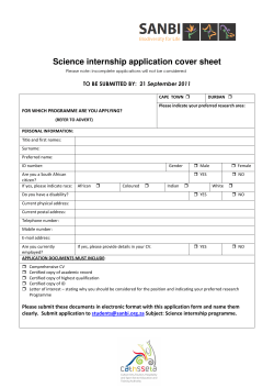


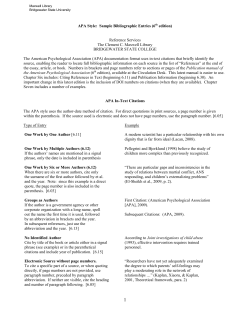
© Copyright 2026