1. No category

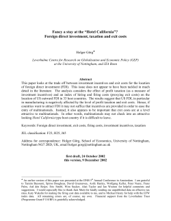
International Journal of Economics, Commerce and Management
United Kingdom
Vol. II, Issue 10, Oct 2014
http://ijecm.co.uk/
ISSN 2348 0386
DETERMINANTS OF FOREIGN DIRECT INVESTMENT IN
BANGLADESH: AN ECONOMETRIC ESTIMATION
Aziz, Md. Shawkatul Islam
Department of Business Administration, World University of Bangladesh, Bangladesh
[email protected]
Ahmed, Mudabber
Department of Economics, University of Chittagong, Bangladesh
[email protected]
Mahmud, Md. Abdul Latif
Department of Business Administration, World University of Bangladesh, Bangladesh
[email protected]
Sarkar, Prosannajid
Dr. Wazed Research Institute, Begum Rokeya University, Rangpur, Bangladesh
[email protected]
Abstract
This study examines the various economic factors effects on foreign direct investment
(FDI) inflows into Bangladesh during the study period ranging from 1972 to 2010. Log
linear regression model has been used and the method of least squares (OLS) has been
applied
to estimate
the
various determinants effects on
FDI inflows. In the models,
dependent variable is Natural Log of real foreign direct investment. Independent variables are
market size proxied by natural log of real GDP, Trade Balance, Labor productivity expressed by
natural log of productivity indices of industrial labor in selected industries (Jute, Cotton, Paper,
Steel, Cement, and Fertilizer). According to the econometric results, market size has positive
sign and is statistically significant. Trade balance is found positive sign and statistically
significant. Labor productivity has positive sign but not significant.
Keyword: Foreign Direct Investment, Determinants of FDI, Unit Root Test, OLS
Licensed under Creative Common
Page 1
© Ahmed, Mahmud & Sarkar
INTRODUCTION
Economic growth in every country depends upon the sustain growth of captive capacity,
supported by savings and investment. Low levels of savings and investment particularly in
developing countries and least developed countries results in a low level of capital stock and
economic growth. Bangladesh which was known as a third world country during the era of cold
war, is now either called a “developing country” or in world bank vocabulary “a low income
country”. With a population of more than 130 million and per capita GDP below US$400, we
need to attract Foreign Direct Investment (FDI) to create employment, generate income and FDI
is considered as a crucial ingredient for economic development of a developing country and can
play an important role in achieving the countries socio-economic objectives including poverty
reduction goals. Countries that are lagging behind to attract FDI are now formulating and
implementing new policies for attracting more investment. Industrial development is one of the
pre-requisites for economic growth, particularly in a developing country. Moving from the
agrarian economy to industrial economy is imperative for economic development. Bangladesh is
an example in this regard. In a capital poor country like Bangladesh FDI can emerge as a
significant vehicle to build up physical capital, create employment opportunities, developed
productive capacity, enhance skills of local labor through transfer of technology and managerial
know-how and help integrate the domestic economy with the global economy.
The determinants which play as a driving force for attracting FDI are geographical
location, cheap labor cost & Government attitude towards liberalization of the existing laws of
the host country, skilled manpower, incentives for investors& exemption of taxes. The objectives
of the study are:
 To evaluate the trend of FDI inflows in Bangladesh;
 To highlight the incentives and facilities provided by the Government institutions for
encouraging FDI in Bangladesh;
 To identify the main determinants of FDI inflows in Bangladesh as a developing country
based on time series data;
 To suggest policy measures for the improvement of foreign direct investment based on
the empirical results.
LITERATURE REVIEW
FDI is considered as an important tool for economic development in a developing country. If the
investing country is wealthier than the host country then capital will flow to the host country
(Zhao, 2003). It contributes to growth of GDP; create employment generation, technology
transfer, human resource development, etc. It is also perceived that FDI can play a significant
role to reduce poverty of a developing country.
Licensed under Creative Common
Page 2
International Journal of Economics, Commerce and Management, United Kingdom
Foreign Direct Investment can be defined as investment in which a firm acquires a substantial
controlling interest in a foreign firm or set up a subsidiary in a foreign country (Chen, 2000). IMF
(1993, 2003) and OECD (1996) defined FDI as a long term investment by a foreign investor in
an enterprise resident in an economy other than foreign direct investor is based. According to
the Balance of Payment Manual (1977 and 1993) FDI refers to investment made to acquire
lasting interest in enterprises operating outside of the economy of the investor.
In the developing world, the East Asian countries - South Korea, Hong Kong, Taiwan
and Singapore were the first to use effectively the FDI from TNCs to achieve economic
development (Sinha, 2007). After opening up their economy towards FDI, these countries
emerged as ‘Asian Tigers’ and witnessed rapid economic developed within a relatively short
period of time. In recent years, many countries have introduced open door policy to attract FDI
with a view to increase investment, employment, productivity and economic development
(Agiomirgianakis et al., 2003). A number of empirical studies have shown that developed and
developing countries both desire to attract FDI. Developing countries always are in
disadvantage in terms of technology, capital, and human resources at the early stage of
development.
In FDI literature it is already recognized that FDI not only brings capital for productive
development to the host economy, it also transfers a considerable amount of technical and
managerial knowledge and skills, which is likely to spill over to domestic enterprise in that
economy (Balasubramanyam et al 1996; Kumar and Podhan,2002). It is recognized that FDI
can contribute to the growth of GDP, Gross Fixed Capital Formation (GFCF) (total investment in
a host economy) and balance of payments (Baskaran and Muchie, 2008).
Most Developing countries are always at a disadvantaged position in terms of
technology and in this regard FDI contribute to transfer technology and can contribute towards
income, production, prices, employment, economic growth, development and general welfare of
the host country (Kok and Ersoy, 2009).
Agiomirgianakis et al (2003) suggested that as FDI increases the total output of the host
country, it eventually contributes to the economic development of the host country. To achieve
industrial expansion a country should produce high quality products and accomplish market
efficiency. To facilitate this technological development is imperative. A developing country like
Bangladesh that is at an early stage of development has to rely on FDI as an important vehicle
to bring in technological development. Hence, it is perceived that FDI is capable of increasing
the technical capabilities of the host country.
According to Sun (1998) FDI has extensively helped economic growth in China by
enriching domestic capital formation, increasing exports, and creating new employment.
Licensed under Creative Common
Page 3
© Ahmed, Mahmud & Sarkar
Khoda (2003) stated that FDI can raise domestic capital, engender employment by using
underutilized labor, build up organizational formation as well as managerial standards of the
host country, transfer technology, get better internal and overseas marketing network and also
assist to improve the technical expertise of the Government. It is argued that “MNEs are subject
to use up more on R&D abroad than at home and their foreign affiliates act comparatively better
in terms of productivity” (Chen, 2000, p. 37). Mmieh and Frimpong (2004) study on the FDI
experience in Ghana reveals that the economic reform has contributed to attracting significant
multinational investment. They also stated that changes to policies and regulations have helped
to increase FDI inflow in China, India, Korea and Mexico.
Agrawal (2000) scrutinized the economic impact of Foreign Direct Investment in South
Asia by undertaking time- series, cross- section analysis of panel data from five South Asian
countries; India, Pakistan, Bangladesh, Sri Lanka and Nepal, and concluded that there existed
complementarily and linkage effects between foreign and national investment. However, using
time series data from the Sri Lankan economy, Athukorala (2003) showed that FDI inflows did
not exert an independent influence on economic growth and the direction of causation was not
towards from FDI to GDP growth but GDP growth and the direction of causation was not
towards from FDI to GDP growth but GDP growth to FDI.
Hermes and Lensink (2000) interestingly summarized different channels through which
positive externalities associated with FDI can occur namely: i) competition channel where
increased competition is likely lead to increased productivity, efficiency and investment in
human and/or physical capital. Increased competition may lead to changes in the industrial
structure towards more competitiveness and more export-oriented activities; ii) training channel
through increased training of labour and management; iii) linkages channel whereby foreign
investment is often accompanied by technology transfer; such transfers may take place through
transactions with foreign firms and iv) domestic firms imitate the more advanced technologies
used by foreign firms commonly termed as the demonstration channel.
Lan (2006) compared Vietnam to other developing countries applying a simultaneous
equation model to test the relationship between FDI and economic growth whose finding was
that FDI had a positive and statistically significant impact on economic growth in Vietnam over
period 1996-2003, and economic growth in Vietnam was viewed as an important factor to entice
FDI inflows into Vietnam. Taking account of macroeconomic environments (degree of trade
openness, income per capita and macroeconomic stability in MENA countries), Jallab, Gbakou,
and Sandretto (2008) assessed the growth-effect of FDI, using data from MENA countries on
period 1970-2005 and summarized that there was no significant independent impact of FDI on
Licensed under Creative Common
Page 4
International Journal of Economics, Commerce and Management, United Kingdom
economic growth in MENA countries. Even, the lack of growth effect of FDI did not depend on
the degree of trade openness and income per capita.
Kindleberger (1969) provided theoretical evidence that for a foreign-owned firm, it is not
a good condition for FDI if the firm has the option of licensing the advantage to an indigenous
producer and product is exported to host country. Due to tariff or transport cost barriers, it will
not be possible and profitable although the other conditions have to be fulfilled for raising FDI.
He pointed out that a company’s final investment decision is usually based on low taxation once
a venture takes off the ground. Besides, a company must have the ability to source goods and
services from its operating unit in one market in order to serve nearby markets or maximize its
global efficiency.
FDI Trend in Bangladesh
Figure-1: FDI Trend during 1995-2010 (US $ in million):
1200
1000
800
600
400
200
0
1995 1996 1997 1998 1999 2000 2001 2002 2003 2004 2005 2006 2007 2008 2009 2010
Source: Various Statistical Year Book Bangladesh (1995-2010)
This graph portrays inconsistent proceedings of the FDI in Bangladesh since 1995. It is a matter
of great concern that in spite of comparative advantages in labor-intensive industries and
adoption of investment friendly policies and regulations, FDI flows have failed to be accelerated.
However, the year 2002 shows a substantial improvement in FDI achievement.
Licensed under Creative Common
Page 5
© Ahmed, Mahmud & Sarkar
METHODOLOGY
The study is based on secondary data and the data is drawn from different sources comprise
time series data of Bangladesh period of 1972-2010.The data sources include annual reports
of different government institutions, concerned ministries and concerned corporate offices,
research journals, investment surveys conducted by BOI, statistical year book of Bangladesh,
publications of BOI and BEPZA, World Investment Reports of UNCTAD, Economic survey of
Bangladesh and previous studies in the field of study. Some information has also been collected
from the daily newspapers and internet sources. All the secondary data collected from printed
materials of the BOI, different government agencies, websites and all other sources. All these
sources of data are recognized and accepted by all and the provided information have been
used widely in the country, so data and information of these sources incorporated in this project
are reliable.
Different time series econometric and inferential statistical techniques were used to
validate the result, where every technique has some pros and cons relating to estimation and
using different methods in same study can bring a robust answer. The inferential statistics, such
as regression, correlation, stationary test (unit root), hypothesis testing and other techniques of
econometric analysis have been used in this study.
Country-specific studies on the south-Asian region find that FDI inflow to south-Asian
countries has been affected by structural factor such as Market size, GDP Growth rate, inflation
rate, Extent of urbanization, Availability of quality infrastructure, Investment incentives and
Performance requirements. Thus, most of the relevant variables considered are based on the
theories and the previous empirical literatures for examining the determinants of FDI in
Bangladesh. After reviewing all the potential determinants of FDI, we adopt the final FDI
function below:
ln(FDI)t = β0+β1MKTSZt + β2TRDBLNt + β3LBRPRDt+ Ut
Ut is the error term with white noise properties and β 0 is a scalar parameter, β1-β3, are the
parameters of interest. Other factor which have influence on inward FDI, neglecting here for
modeling difficulty and lack of appropriate data availability for the assigned study period.
Variable Definitions and Data Sources
1.
ln (FDI) = Natural Log of real foreign direct investment registered with BOI (Billions of
taka). Source: Bangladesh Investment Handbook, 2010 and previous issues and UNCTAD,
World Invest Report-2008.
2.
MKTSZ = Host country market size proxied by natural log of real GDP (Billions of taka).
Source: Statistical year book of Bangladesh (BBS), 1981, 1991, 2001, 2008, 2010.
Licensed under Creative Common
Page 6
International Journal of Economics, Commerce and Management, United Kingdom
3.
TRDBLN = Host country Trade Balance (Export- import) (Billions of taka) Source:
www.adb.org/statistics. Bangladesh Economic Review, 2011.
4.
LBRPRD = Labor productivity, expressed by natural log of productivity indices of
industrial labor in selected industries (Jute, Cotton, Paper, Steel, Cement, Fertilizer). Source:
Statistical year book of Bangladesh (BBS), 1981, 1991, 2001, 2007, 2010.
Domestic market characteristics are expressed by the market size and trade flows. The market
size (MKTSZ) is measured by the host country real GDP and emphasizes the importance of a
large market for efficient utilization of resources. A direct relationship is expected between
MKTSZ and inward FDI. The relationship between the direction of the host country trade
balance (TRDBLN) and FDI inflow appears to be complex. Trade surpluses are indicative of a
strong economy and may encourage the inflow of FDI. Trade deficits, on the other hand, may
stimulate inward FDI as a result of export diversification and import substitution policies. Labor
productivity (LBRPRD) is expected to directly affect the ability of the host country to attract FDI.
EMPIRICAL ANALYSIS
The Unit Root Test
A test of stationarity or non-stationary that has become widely popular over the past several
years is the unit root test. So we use Dickey-Fuller (DF) test to operate the unit root test. We
consider following equation;
ΔYt = β1+δYt-1+Ut
Both hypotheses are,
H0: δ = 0
[Time series is non-stationary]
Ha: δ < 0
[Time series is stationary]
If the null hypothesis is rejected, it means that Yt is a stationary time series. Dickey-Fuller have
shown that under the null hypothesis that δ =0, the estimated value t value of the coefficient of
Yt-1 in above equation follows the  (tau) statistic (D.N. Gujarati, 1995). The computed p- value
is less than even the 5 percent critical value in absolute terms then null hypothesis is accepted
and conclusion is that the time series is non-stationary. The unit root test results are shown in
Table 1 (According to Appendix-1).
Licensed under Creative Common
Page 7
© Ahmed, Mahmud & Sarkar
Table-1: Results of unit root test
VARIABLE
P-VALUE
Ln(FDI)
NULL
HYPOTHESIS
A(1)=0,T-TEST
DECESION
0.1651
CRITICAL VALUE
5%
0.05
MKTSZ
A(1)=0, T-TEST
0.9998
0.05
H0 accepted
TRDBNL
A(1)=0, T-TEST
1.0000
0.05
H0 accepted
LBRPRD
A(1)=0, T-TEST
0.7759
0.05
H0 accepted
H0 accepted
Here dependent variable ln(FDI) and other independent variables such as MKTSZ, TRDBLN
and LBRPRD, all are individually I(1); that is they are non-stationary an contain a unit root. So
the regression of a non-stationary time series on other non-stationary time series may produce
a spurious regression. Though all variables are non-stationary, but if all independent variables
are co-integrated with the dependent variable ln(FDI), then the produced regression will not
spurious. So we have to operate co-integration technique with help of E-VIEWS.
Co-Integration Test
Table-2: Results of co-integration test (According to Appendix-2)
COINTEGRATING REGRESSION-CONSTANT, TREND NO. OBS, 38
Co-integration between
REGRESSAND: ln(FDI)
ln(FDI) & all independent
R-SQUARE=0.329
DURBIN-WATSON=2.07
variables
P-VALUE
CRITICAL VALUE 5%
T-TEST
0.0021
0.05
Decision: MKTSZ, TRDBLN, and LBRPRD all are co-integrated with
dependent variable ln(FDI)
The result indicates us that we can reject the null. It means that the variables are co integrated.
So if we apply OLS method, regression result of this model will not spurious.
Licensed under Creative Common
Page 8
International Journal of Economics, Commerce and Management, United Kingdom
Descriptive statistics of major variables
With the help of E-views, the descriptive statistics of ln (FDI), MKTSZ, TRDBLN, LBRPRD are
as follows:
Table- 3: Descriptive statistics
ln(FDI)
MKTSZ
TRDBLN
LBRPRD
Mean
1.255591
7.287130
-110.8872
4.838070
Median
1.444563
7.229955
-64.00000
4.849997
Maximum
4.962425
8.188820
-0.140000
5.565991
Minimum
-4.605170
6.489995
-364.6400
3.599775
Std. Dev.
2.611676
0.500763
112.3693
0.530624
Skewness
-0.507957
0.199321
-1.013679
-0.680278
Kurtosis
2.321303
1.884343
2.833744
2.854444
Jarque-Bera
2.425658
2.280858
6.723963
3.042482
Probability
0.297355
0.319682
0.034667
0.218441
Sum
48.96805
284.1981
-4324.600
188.6847
Sum Sq. Dev.
259.1924
9.529005
479820.8
10.69934
Observations
39
39
39
39
From the Table-3 it is seen that the frequency distributions of all major variables are not normal.
The skewness coefficient is less then unity, generally taken to be fairly extreme (Chou, 1988,
P.109). Statistician Kendall (1943) calculated the expected normal kurtosis equal to 3(n1)/(n+1), where, n=Sample Size. According to this rule in a Guassian distribution, it can be
calculated for these data to have a kurtosis co-efficient of 2.846 for all the major variables
respectively. Kurtosis generally either much higher or lower than the above calculated values
indicates extreme leptokurtic or extreme platykurtic.
In this data set, the value of 2.321, 1.884, 2.833and 2.854 for ln(FDI), MKTSZ, TRDBLN
and LBRPRD respectively fall under the platykurtic distribution. Generally values for skewness
zero (β1=0) and kurtosis value 3 (β2=3) indicate that the observed distribution is perfectly
normally distributed. Therefore skewness and platykurtic frequency distribution of major
variables on FDI indicates that the distribution is not normal.
Licensed under Creative Common
Page 9
© Ahmed, Mahmud & Sarkar
OLS Estimation
Estimated results with Ordinary Least Square method has been reported in Table-4. (According
to Appendix -3), along with the model summery in Table 5 and ANOVA results in Table 6.
Table -4: Regression Results
Coefficient
Std. Error
t-Statistic
Prob.
C
-54.33731
8.664915
-6.270957
0.0000
MKTSZ
7.855486
1.463339
5.368191
0.0000
TRDBLN
0.015921
0.005533
2.877393
0.0068
LBRPRD
0.023645
0.778855
0.030359
0.9760
Table-5: Model Summary
R
.891
R Square
Adjusted R Square
.793
.775
Std. Error
Estimate
1.239
of the
Durbin-Watson
1.24
Table-6: ANOVA
Model
Regression
Residual
Total
Sum
Squares
205.84
of
df
Mean Square
F
Sig.
3
68.6
44.61
.000
53.73
35
1.54
259.57
38
The fitted line is reasonably good. The goodness of fit, R 2 shows that the independent variables
explain about 79.30% of the variations in the dependent variable. The estimated coefficients
have all expected sings except TRDBLN. The coefficient of the Market Size is 7.86, implying
that a one percent increase in total Market Size increases the FDI by 7.86 percent. Similarly a
one percent increase in Labor Productivity will increase the FDI by 0.02 percent. Since, the sign
of TRDBLN is not expected. So, we cannot explain the effect of TRDBLN in this model. The
estimated regression equation is reproduced below:
ln (FDI)= -54.337+7.855MKTSZ+0.015TRDBLN+0.023LBRPRD
The results show that MKTSZ (natural log of Real GDP) is the most significant factor affecting
FDI inflow into the Bangladesh. We get positive sign and statistically significant. In Bangladesh
trade deficit is a continuous process, so negative sign is expected but we get positive sign and
statistically significant. Labor productivity (LBRPRD), which is one of the major determinants of
FDI in Bangladesh, is statistically insignificant.
Licensed under Creative Common
Page 10
International Journal of Economics, Commerce and Management, United Kingdom
The “F” test
The null and alternative hypothesis are:
Ho: β1 = β2 = β3 =0
Ha: β1 = β2= β3 ≠0
(i.e. β1, β2, β 3 are not simultaneously zero)
According to Appendix-3 the calculated ‘F’ value is 44.61 while the critical value of ‘F’ is 2.87 at
the 5% level of significance with (3, 35) df. As a result the null hypothesis is rejected. That is,
the estimated equation is significant.
Test for Functional form and Omitted variables
Ramsey’s “RESET” test can be used to this purpose. Reset stands for Regression Specification
Error Test and was proposed by Ramsey (1969). RESET is a general test for the following types
of specification errors:
Omitting variables included irrelevant ones, chosen a wrong functional form and
correlation between explanatory variables and error term. The test procedure is as follows:
Firstly the original equation:
ln(FDI)t = β0+β1MKTSZt + β2TRDBLNt + β3LBRPRDt+ Ut
is run and from the estimated equation fitted values of ln(FDI) i.e. ln(FDI) i is obtained. And then
the following regression is run:
ln(FDI)t = β0+β1MKTSZt + β2TRDBLNt + β3LBRPRDt+δ1ln(FDI)2+
δ2ln(FDI)3 +Vt
HO:δ1=δ2=0;
Fcal=37.32>3.30;and p-value(0.000)<0.05
(According to Appendix-4)
Now δ1and δ2 are statistically insignificant then it can be concluded that there is no problem with
functional form or omitted variables. So, we can say that this model does not contain serious
problem of functional form and omitted variable.
Jarque –Bera test
We can compute Jarque-Bera test statistic using the following rule:
JB=n[S 2/6+ (K-3)2/24]
Where S represents skewness and K represents kurtosis. In our model, skewness and kurtosis
values of residuals are 0.29 and 2.20 respectively. By using Jarque-Bera test computed
JB=1.57, which is less than the critical value of 5.99 at 5% level of significance with 2 df, Which
Licensed under Creative Common
Page 11
© Ahmed, Mahmud & Sarkar
shown in figure-2. We also fail to reject the null hypothesis on the grounds that 0.456 > 0.05.So
this model does not violate the normality assumption.
Figure-2: Jarque –Bera test estimation
7
Series: Residuals
Sample 1 39
Observations 39
6
5
4
3
2
1
Mean
Median
Maximum
Minimum
Std. Dev.
Skewness
Kurtosis
-7.62e-15
-0.092832
2.788506
-1.873772
1.189116
0.291986
2.209888
Jarque-Bera
Probability
1.568612
0.456436
0
-2
-1
0
1
2
3
Tests for Heteroskedasticity
Homoskedasticity is an important property for OLS method. So it is important to find out whether
there is any heteroskedasticity problem or not. To test heteroskedasticity, we have used the
“Breusch–Pagan-Godfrey Test”.
The “Breusch–Pagan-Godfrey Test”
Here the null and alternative hypotheses are;
Ho: There is no heteroskedasticity
Ha: There is heteroskedasticity problem
The formula of the Breusch-Pagan-Godfrey test shows as follows:
χ2=N*R2 ~ asy χ2 (s-1)
Where χ2 shows chi-square distribution with (s-1) degrees of freedom
Our observed χ2 = 2.93. Now, we find that for 3 df and 5% level of significance, critical χ2 =
7.815 and the 1% critical χ2 = 11.345. Thus the observed χ2 = 2.93 is not significant at 1% as
well as 5% level of significance. So the model is free from heteroskedasticity problem
(According to appendix-5).
Licensed under Creative Common
Page 12
International Journal of Economics, Commerce and Management, United Kingdom
Test for Autocorrelation
In order to conduct Durbin-Watson test statistic, following assumptions must be satisfied:
1) It is necessary to include a constant term in the regression.
2) The explanatory variables are non-stochastic, in repeated sampling.
3) The disturbance terms Ut are generated by the first order auto-regressive scheme.
4) The regression model does not include lagged values of the dependent variable as one of the
explanatory variables.
5) There are no missing observations in data.
6) The error term Ut is assumed to be normally distributed.
In the absence of software that computes a p-value, a test known as the bounds test can be
used partially overcome the problem of not having general critical values Durbin & Watson
considered two other statics d l & du whose probability distribution do not depend on the
explanatory variables and which have the property that
dl < d < du
That is, irrespective of the explanatory variables in the model under consideration will be
bounded by an upper bound d u and 0 a lower bound dl. If d < dl H0 is rejected and d >du is not
rejected. Our regression model is qualified by all these assumptions. So, we can use DurbinWatson test. The test procedure is as follows:
Ho: ρ=0 (No auto correlation)
Ha: ρ≠ 0 ( auto correlation)
For this model, we have estimated d= 1.24, against for n=39, k=3 and α=5%, the d L= 1.328 and
du= 1.658, Here 5% significance level, du = 1.658 and estimated d= 1.24. So we can reject H 0
because of d<du. That is statistically significant evidence of positive autocorrelation. (Acoording
to Appendix-3)
For reducing this problem, we can apply “Cochrane-Orcutt” iterative procedure to
estimate ρ, where, ρ is known as the coefficient of auto-covariance. After that we can have a
conclusion with the help of EGLS technique.
Tests for Multicollinearity: Correlation matrix
Multicollinearity is a sample phenomenon; we don’t have a unique method of testing
multicollinearity. For detecting multicollinearity in our model, we use E-VIEWS.
Correlation matrix is one of the best techniques to detect multicollinearity. Now let’s have
a look at the following correlation matrix.
Licensed under Creative Common
Page 13
© Ahmed, Mahmud & Sarkar
Table-7: Correlation matrix
MKTSZ
TRDBLN
LBRPRD
MKTSZ
1.000000
-0.946181
0.873459
TRDBLN
-0.946181
1.000000
-0.818964
LBRPRD
0.873459
-0.818964
1.000000
According to the Table-7, it can be seen that some variables are highly correlated with one
another. Particularly, the correlated co-efficient between MKTSZ and LBRPRD, These values
are .873, respectively suggesting that the variable pair is highly correlated which are greater
than 0.8. That is multicollinearity problem exists in this model.
So we can see, several of these pair-wise correlations are quite high, suggesting that
there may be a several collinearity problem. Of course, remember the warning given earlier that
such pair-wise correlations may be sufficient but not a necessary condition for the existence of
multicollinearity.
CONCLUSIONS AND POLICY IMPLICATIONS
Foreign direct investment (FDI) is a powerful weapon of economic development especially in the
current global context. It enables a capital poor country like Bangladesh to build up physical
capital, create employment opportunities, develop productive capacity, enhance skills of local
labor through transfer of technology and managerial proficiency and help integrate the domestic
economy with the global economy.
By recovering the gap between domestic savings and investments and by enhancing
technical knowledge spread out, FDI can play important role in industrial development and
economic growth in Bangladesh. Although most of the developing countries have been taking
measures to attract FDI, but only a few countries are doing well in attracting FDI inflow.
One of the objectives of this study was to find out the determinant of foreign direct
investment inflows in Bangladesh. In order to ascertain the determinants of FDI, this study
undertakes an econometric study based on time series data for Bangladesh for the period of
1972-2010. The results from the co-integration tests reveal that FDI in Bangladesh and all its
potential determinants have a long-run relationship, because all independent variables are cointegrated with FDI in our model.
The major determinants of FDI in Bangladesh are market size as measured by real GDP
(MKTSZ), Trade Balance (TRDBNL) and labor productivity (LBRPRD), but MKTSZ and
TRDBLN are found to be statistically significant in the original model.
Licensed under Creative Common
Page 14
International Journal of Economics, Commerce and Management, United Kingdom
Based on empirical findings, it is suggested that Bangladesh should try to improve or expand its
market size, and improve labor productivity by giving institutional and vocational education
among the mass people for attracting more FDI into the country. The importance of FDI cannot
be overstated. As a result the investment climate in the country must be improved through
appropriate measures.

Crating more transference in the trade policy and more flexible and setting a
suitable regulatory framework and tariff structure.

Developing the port (Chittagong and Khulna) network, road network, railways
and telecommunications facilities etc.

Particular reforms measures are needed in the administrative system.
Bureaucratic control and interference in business and investment activities
should be minimized.

As a developing country Bangladesh should maintain a good relation with the
developed as well as the developing countries for receiving significant share of
total FDI.

Finally, political risks and instability must be reduced for raising the confidence of
foreign investors. Opposition can play a vital role in that context.
FURTHER RESEARCH
The simple model we developed in this study may suffer from a number of shortcomings.
Therefore, some venues for future research may be considered. They are as follows:
This study uses annual time series data, which may mask some important dynamic aspects. An
analysis based on quarterly or monthly data should certainly be more enriching. But availability
of monthly data for Bangladesh would continue to be a major stumbling block at least in the
foreseeable future. An important driving force of future research in time series analysis is the
advance in high-volume data acquisition. Examples are: transaction-by-transaction data
common to financial markets or communications networks, and in e-commerce on the internet.
These data will be available in future and must be processed properly and efficiently. But the
special features of the data, such as large sample sizes, heavy tails, unequally spaced
observations, and mixtures of multivariate discrete and continuous variables, can easily render
existing methods inadequate. Analyses of these types of data will certainly influence the
directions of future research.
Licensed under Creative Common
Page 15
© Ahmed, Mahmud & Sarkar
REFERENCES
Ahmad,M.G. and Tanin,F.,(2010), “Determinants of ,and the relationship between FDI and economic
growth in Bangladesh.” UDC.
Asiedu, E. (2002). “On the determinants of foreign direct investment to developing countries: is Africa
different?” World Development, 30, 107–119.
Asiedu, E. (2006), “Foreign direct investment in Africa: The role of natural resources, market size,
government policy, institutions and political instability”, World Economy, 29 (1), 63-77.
Asiedu, E., & Esfahani, H. S. (2001). “Ownership structure in foreign direct investment projects. Review of
Economics and Statistics”, 83, 647–662.
Assuncao, S., Forte, R. and Teixeira, A. A. C., “Location determinants of FDI : A literature review, PEP
Working Papers, no. 433, October 2011.
Azam, M. and Lukman, L. “Determinants of foreign derect investment in India, Indonesia and Pakistan: A
quantitative approach, Journal of Managerial Sciences, vol. 4, no. 1.
Baltagi, B. H. (2001). “Econometric analysis of panel data”. New York: Wiley.
Barkat, Abul “Political Economy of Investment Climate in Bangladesh: When Structure Impedes
Progress”, Bangladesh Journal of Political Economy, Volume 22, 2005, pp. 293-294.
Barkat, Abul “Political Economy of Investment Climate in Bangladesh: When Structure Impedes
Progress”, Bangladesh Journal of Political Economy, Volume 22, 2005, pp. 294.
Bhavan, T., Xu, C. and Zhong, C., “Determinants and growth effect of FDI in South Asian Economies :
Evidence from a panel data analysis, International Business Research, Vol.4, No. 1; January 2011.
Blomiger, B. A., “A review of the empirical literature on FDI determinants” (April. 2005).
Blomstronm, M., Globerman, S. and Kokko, A., “The determinants of host country spillovers from foreign
direct investment : Review and synthesis of the literature, Working Paper , no. 76, September 1999.
Brunetti, A., Kisunko, G., & Weder, B. (1997). “Institutional obstacles to doing business: region-by-region
results from a worldwide survey of the private sector.” World Bank Policy Research Working Paper 1759,
World Bank, Washington, DC.
Carlson, M., & Hernandez, L. (2002). “Determinants and repercussions of the composition of capital
inflows. Board of Governors of the Federal Reserve System International Finance Discussion”, Paper
Number 717, Federal Reserve System, New York.
Chou, R. (1988), “Volatility persistence and stock valuation; Some Empirical Evidence Using GARCH”,
Journal of Applied Econometrics, pp. 109.
Damodar N. Gujarati, “Basic Econometrics”, fourth edition, 2003
Damodar N. Gujarati, “Basic Econometrics”, third edition, 1995.
Demirhan, E. and Masca, M., “Determinants of foreign direct investment flows to developing countries: A
cross - sectional analysis”, PRAGUE Economic Papers, 4, 2008,
Hussain, F. and Kimuli, C. B., “Determinants of foreign direct investment flows to developing countries”,
SBR Research Bulletin, Vol.8, No. 1, 2012.
Johnston, J. “Econometric Methods”, second edition, 1992.
Judge, G.G., W.E. Griffiths, R.C. Hill, H. Lutkepohl and T.C. Lee (1985) “The Theory and Practice of
Econometrics”, second edition.
Kendall, M.G., (1943), “The Advanced Theory of Statistics”, Vol. 1, London; Griffin.
ODI Briefing Paper “Foreign Direct Investment flows to low-income countries: A review of the evidence”,
1997(3), September, Pp. 3-5.
Licensed under Creative Common
Page 16
International Journal of Economics, Commerce and Management, United Kingdom
Pindyck, R. S. and Rubinfeld, D.L. “Econometrics Models and Economic Forecasts”, second edition,
1981.
Reza Sadrel and M. Ali Rashid, “Foreign Direct Investment: Problems and Prospects in the Bangladesh
Economy in Transition” M. G. Quibria, United Press Ltd, Dhaka, Bangladesh, 1997, pp. 202.
Reza Sadrel, Rashid M. Ali and Alam A. H. M. Mahbubul, 1987 “Private Foreign Investment In
Bangladesh”, University Press Ltd, pp. 29-30.
Reza Sadrel, Rashid M. Ali and Alam A. H. M. Mahbubul, 1987 “Private Foreign Investment In
Bangladesh”, University Press Ltd, pp. 68-69.
Sahoo, Provakar, “Foreign Direct Investment in South Asia: Policy, Trends, Impacts and Determinants”,
ADB Institute Discussion Paper, No. 56, Nov. 2006, pp. 18.
Shamsuddin, A. F. M., “Economic determinants of foreign direct investment in less developed countries,
The Pakistan Development Review, 33:1(spring 1994), pp.41-51.
Sobhani F. A., “Inflow of Foreign Direct Investment in Bangladesh a trend analysis”, Chittagong
International Trade Fair-2005, CCCI, Chittagong, Bangladesh, 2005, Pp. 22-26.
Statistical Year book of Bangladesh (BBS), Issues 1981, 1991, 2001, 2008and 2010.
Uddin,M.M.,(2002), “Bangladesh Business Year Book”.
UNCTAD, “World Investment Report”, United Nations: New York and Geneva, 2006.
Walsh, J. P. and Yu, J. (July 2010), “Determinants of foreign direct investment : A sectoral and
institutional approach, IMF Working Paper, Asia Pacific Department.
Wan, X. (2010), “A literature review on the relationship between foreign direct investment and economic
growth, International Business Research, vol. 3, no. 1, January 2010.
Wang, Z and N. Swain, “The Determinants of FDI in Transforming Economies: Empirical Evidence from
Hungary and China”, welt wirtschaftiches, Vol. 129, Pp. 359-381.
APPENDICES
Appendix-1
Null Hypothesis: X1 has a unit root
Exogenous: Constant
Lag Length: 0 (Automatic based on SIC, MAXLAG=9)
Augmented Dickey-Fuller test statistic
Test critical values:
1% level
5% level
10% level
t-Statistic
Prob.*
-2.340535
-3.615588
-2.941145
-2.609066
0.1651
*MacKinnon (1996) one-sided p-values.
Augmented Dickey-Fuller Test Equation
Dependent Variable: D(X1)
Method: Least Squares
Date: 09/13/12 Time: 13:58
Licensed under Creative Common
Page 17
© Ahmed, Mahmud & Sarkar
Sample (adjusted): 2 39
Included observations: 38 after adjustments
X1(-1)
C
R-squared
Adjusted R-squared
S.E. of regression
Sum squared resid
Log likelihood
F-statistic
Prob(F-statistic)
Coefficient
Std. Error
t-Statistic
Prob.
-0.190159
0.454515
0.081246
0.229615
-2.340535
1.979463
0.0249
0.0555
0.132072
0.107963
1.286250
59.55982
-62.45817
5.478104
0.024915
Mean dependent var
S.D. dependent var
Akaike info criterion
Schwarz criterion
Hannan-Quinn criter.
Durbin-Watson stat
0.230199
1.361865
3.392535
3.478724
3.423201
2.661677
Null Hypothesis: X2 has a unit root
Exogenous: Constant
Lag Length: 0 (Automatic based on SIC, MAXLAG=9)
Augmented Dickey-Fuller test statistic
Test critical values:
1% level
5% level
10% level
t-Statistic
Prob.*
2.063217
0.9998
-3.615588
-2.941145
-2.609066
*MacKinnon (1996) one-sided p-values.
Augmented Dickey-Fuller Test Equation
Dependent Variable: D(X2)
Method: Least Squares
Date: 09/13/12 Time: 13:59
Sample (adjusted): 2 39
Included observations: 38 after adjustments
X2(-1)
C
R-squared
Adjusted R-squared
S.E. of regression
Sum squared resid
Log likelihood
F-statistic
Prob(F-statistic)
Coefficient
Std. Error
t-Statistic
Prob.
0.010009
-0.027997
0.004851
0.035314
2.063217
-0.792803
0.0464
0.4331
0.105743
0.080902
0.014305
0.007367
108.4989
4.256866
0.046360
Licensed under Creative Common
Mean dependent var
S.D. dependent var
Akaike info criterion
Schwarz criterion
Hannan-Quinn criter.
Durbin-Watson stat
0.044706
0.014921
-5.605205
-5.519016
-5.574540
2.059047
Page 18
International Journal of Economics, Commerce and Management, United Kingdom
Null Hypothesis: X3 has a unit root
Exogenous: Constant
Lag Length: 8 (Automatic based on SIC, MAXLAG=9)
t-Statistic
Augmented Dickey-Fuller test statistic
Test critical values:
3.913058
1% level
5% level
10% level
Prob.*
1.0000
-3.670170
-2.963972
-2.621007
*MacKinnon (1996) one-sided p-values.
Augmented Dickey-Fuller Test Equation
Dependent Variable: D(X3)
Method: Least Squares
Date: 09/13/12 Time: 14:01
Sample (adjusted): 10 39
Included observations: 30 after adjustments
X3(-1)
D(X3(-1))
D(X3(-2))
D(X3(-3))
D(X3(-4))
D(X3(-5))
D(X3(-6))
D(X3(-7))
D(X3(-8))
C
R-squared
Adjusted R-squared
S.E. of regression
Sum squared resid
Log likelihood
F-statistic
Prob(F-statistic)
Licensed under Creative Common
Coefficient
Std. Error
t-Statistic
Prob.
0.505225
-0.936438
-0.863662
-0.950463
-1.393826
-1.106956
-0.520393
-0.951679
-0.620661
-12.28862
0.129113
0.311341
0.287798
0.318597
0.319589
0.343223
0.404564
0.336119
0.375281
5.841219
3.913058
-3.007757
-3.000932
-2.983277
-4.361314
-3.225183
-1.286306
-2.831381
-1.653859
-2.103777
0.0009
0.0070
0.0071
0.0073
0.0003
0.0042
0.2130
0.0103
0.1138
0.0483
0.613789
0.439994
17.37730
6039.413
-122.1411
3.531685
0.008989
Mean dependent var
S.D. dependent var
Akaike info criterion
Schwarz criterion
Hannan-Quinn criter.
Durbin-Watson stat
-11.27967
23.22127
8.809408
9.276474
8.958827
2.117122
Page 19
© Ahmed, Mahmud & Sarkar
Null Hypothesis: X4 has a unit root
Exogenous: Constant
Lag Length: 0 (Automatic based on SIC, MAXLAG=9)
Augmented Dickey-Fuller test statistic
Test critical values:
1% level
5% level
10% level
t-Statistic
Prob.*
-0.904673
-3.615588
-2.941145
-2.609066
0.7759
*MacKinnon (1996) one-sided p-values.
Augmented Dickey-Fuller Test Equation
Dependent Variable: D(X4)
Method: Least Squares
Date: 09/13/12 Time: 14:02
Sample (adjusted): 2 39
Included observations: 38 after adjustments
X4(-1)
C
R-squared
Adjusted R-squared
S.E. of regression
Sum squared resid
Log likelihood
F-statistic
Prob(F-statistic)
Coefficient
Std. Error
t-Statistic
Prob.
-0.058435
0.304932
0.064592
0.313201
-0.904673
0.973597
0.3717
0.3368
0.022229
-0.004931
0.206961
1.541987
6.966112
0.818434
0.371653
Mean dependent var
S.D. dependent var
Akaike info criterion
Schwarz criterion
Hannan-Quinn criter.
Durbin-Watson stat
0.023220
0.206453
-0.261374
-0.175186
-0.230709
2.268148
Appendix-2:
Null Hypothesis: RESID01 has a unit root
Exogenous: Constant
Lag Length: 0 (Automatic based on SIC, MAXLAG=9)
Augmented Dickey-Fuller test statistic
Test critical values:
1% level
5% level
10% level
t-Statistic
Prob.*
-4.196985
-3.615588
-2.941145
-2.609066
0.0021
*MacKinnon (1996) one-sided p-values.
Licensed under Creative Common
Page 20
International Journal of Economics, Commerce and Management, United Kingdom
Augmented Dickey-Fuller Test Equation
Dependent Variable: D(RESID01)
Method: Least Squares
Date: 09/22/12 Time: 06:56
Sample (adjusted): 2 39
Included observations: 38 after adjustments
Coefficient
Std. Error
t-Statistic
Prob.
RESID01(-1)
C
-0.639770
0.033056
0.152436
0.181132
-4.196985
0.182494
0.0002
0.8562
R-squared
Adjusted R-squared
S.E. of regression
Sum squared resid
Log likelihood
F-statistic
Prob(F-statistic)
0.328542
0.309891
1.116554
44.88096
-57.08179
17.61468
0.000169
Mean dependent var
S.D. dependent var
Akaike info criterion
Schwarz criterion
Hannan-Quinn criter.
Durbin-Watson stat
0.028360
1.344067
3.109568
3.195756
3.140233
2.073906
Appendix-3
Dependent Variable: X1
Method: Least Squares
Date: 09/21/12 Time: 20:24
Sample: 1 39
Included observations: 39
C
X2
X3
X4
R-squared
Adjusted R-squared
S.E. of regression
Sum squared resid
Log likelihood
F-statistic
Prob(F-statistic)
Coefficient
Std. Error
t-Statistic
Prob.
-54.33731
7.855486
0.015921
0.023645
8.664915
1.463339
0.005533
0.778855
-6.270957
5.368191
2.877393
0.030359
0.0000
0.0000
0.0068
0.9760
0.792695
0.774926
1.239031
53.73189
-61.58728
44.61111
0.000000
Licensed under Creative Common
Mean dependent var
S.D. dependent var
Akaike info criterion
Schwarz criterion
Hannan-Quinn criter.
Durbin-Watson stat
1.255591
2.611676
3.363450
3.534072
3.424668
1.244543
Page 21
© Ahmed, Mahmud & Sarkar
Appendix-4
Ramsey RESET Test:
F-statistic
Log likelihood ratio
3.997118
4.334842
Prob. F(1,34)
Prob. Chi-Square(1)
0.0536
0.0373
Test Equation:
Dependent Variable: X1
Method: Least Squares
Date: 09/22/12 Time: 06:53
Sample: 1 39
Included observations: 39
C
X2
X3
X4
FITTED^2
R-squared
Adjusted R-squared
S.E. of regression
Sum squared resid
Log likelihood
F-statistic
Prob(F-statistic)
Coefficient
Std. Error
t-Statistic
Prob.
-53.01255
7.538728
0.011065
0.255552
-0.098899
8.342520
1.413350
0.005840
0.756453
0.049467
-6.354502
5.333942
1.894895
0.337829
-1.999279
0.0000
0.0000
0.0666
0.7376
0.0536
0.814502
0.792679
1.189161
48.07954
-59.41986
37.32271
0.000000
Mean dependent var
S.D. dependent var
Akaike info criterion
Schwarz criterion
Hannan-Quinn criter.
Durbin-Watson stat
1.255591
2.611676
3.303583
3.516860
3.380105
1.247555
Appendix-5
Heteroskedasticity Test: Breusch-Pagan-Godfrey
F-statistic
Obs*R-squared
Scaled explained SS
0.948192
2.931423
1.428238
Prob. F(3,35)
Prob. Chi-Square(3)
Prob. Chi-Square(3)
0.4279
0.4023
0.6989
Test Equation:
Dependent Variable: RESID^2
Method: Least Squares
Date: 09/22/12 Time: 06:46
Sample: 1 39
Included observations: 39
Licensed under Creative Common
Page 22
International Journal of Economics, Commerce and Management, United Kingdom
C
X2
X3
X4
R-squared
Adjusted R-squared
S.E. of regression
Sum squared resid
Log likelihood
F-statistic
Prob(F-statistic)
Coefficient
Std. Error
t-Statistic
Prob.
-0.405270
-0.525982
0.004787
1.270495
10.75853
1.816911
0.006870
0.967042
-0.037670
-0.289493
0.696813
1.313796
0.9702
0.7739
0.4905
0.1975
0.075165
-0.004107
1.538405
82.83411
-70.02753
0.948192
0.427924
Licensed under Creative Common
Mean dependent var
S.D. dependent var
Akaike info criterion
Schwarz criterion
Hannan-Quinn criter.
Durbin-Watson stat
1.377741
1.535255
3.796284
3.966905
3.857501
1.985584
Page 23