A mathematical model of cancer treatment by radiotherapy
I
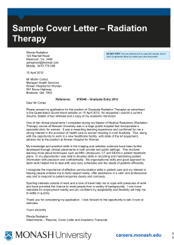
Zijian Liua,b,∗, Chenxue Yangc
a School
of Science, Chongqing Jiaotong University, Chongqing 400074, PR China
of Mathematics, Hangzhou Normal University, Hangzhou, Zhejiang 310036, PR China
c School of Computer Science and Engineering, University of Electronic Science and Technology of China, Chengdu 610054,
PR China
b Department
Abstract
A periodic mathematical model of cancer treatment by radiotherapy is presented and studied in this paper.
Conditions on the coexistence of the healthy and cancer cells are obtained. Furthermore, sufficient conditions
on the existence and globally asymptotic stability of the positive periodic solution, the cancer eradication
periodic solution and the cancer win periodic solution are established. Some numerical examples are shown
to verify the validity of the results. A discussion is presented for further study.
Keywords: Radiotherapy; Periodic of treatment; Coexistence; Cancer eradication periodic solution;
Cancer win periodic solution
1. Introduction
Cancer is a well-known killer of humans world wide, and its treatments are varied and sporadically
successful. There are four main types of cancer treatments, which are surgery, chemotherapy, radiotherapy
and immunotherapy. In this paper, we only consider cancer treatment by radiotherapy.
Radiotherapy, as a primary treatment strategy, has been proven to be an effective tool in combating
with cancer [1, 2]. Radiation therapy is a treatment procedure that uses radiation to kill malignant cells.
This treatment targets rapidly reproducing cells such as those in cancer [3]. Therefore, when cancer cells
are irradiated, there is a lesser effect on more slowly reproducing surrounding healthy cells. As such, the
intent of this paper is to model the dynamics and interactions of healthy and cancer cells under radiation
therapy.
It is an important and effective way to deeply understand the real-world problems by establishing mathematical models and analyzing their dynamical behaviors (see [4, 5, 6, 7, 8, 9] and reference cited therein).
Recently, some mathematical models that focus on cancer treatment by radiotherapy have been presented
I This research was supported by the National Natural Science Foundation of China (11401060) and Zhejiang Provincial
Natural Science Foundation of China (LQ13A010023).
∗ Corresponding author
Email addresses: [email protected] (Zijian Liu), [email protected] (Chenxue Yang)
1 Tel. +86 18225022503; fax: +86 23 62652254
Preprint submitted to Computational and Mathematical Methods in Medicine
October 24, 2014
and studied ([10, 11, 12, 13]). Liu and Zhong in [10] focused on dynamical behaviors of normal cells that
affected by periodic radiation and established some conditions on the permanence and extinction of the
normal and radiated cells. Moreover, they obtained criteria on the existence and global asymptotic stability
of unique positive periodic solutions of the system. Belostotski in [11] presented a mathematical model
to represent the interactions between healthy and cancer cells subject to radiation, where the interactions
between healthy and cancer cells were viewed as competition for bodily resources. He featured four different
control mechanisms of radiation delivery. They included continuous constant radiation, continuous radiation
that is proportional to the instantaneous cancer concentration, continuous radiation that is proportional to
the ratio of cancer to healthy cell concentration, and periodic administration of radiation. He supposed
that the effect of radiation on healthy cells ideally is zero and obtained some sufficient conditions on each
cases that guarantee the cancer to be cure or treatment. In paper [12], Belostotski and Freedman developed
and analyzed a mathematical model of cancer treatment by radiotherapy using control theory, where the
radioactivity only affected the cancer cells. Later, considering the fact that the radiation also may affect the
healthy cells to some extent during the radiotherapy, Freedman and Belostotski in [13] extended the previous
study by perturbing the previous models. They considered four types of treatment delivery: constant, linear,
feedback and perturbed periodic deliveries. For each case, they established some sufficient conditions on
the cure state and treatment state. However, paper [13] only considered the perturbed periodic radiation,
although paper [12] investigated the periodic radiation, it supposed that the effect of radiation on healthy
cells is zero. Hence, the study of periodic radiation under conditions that both the cancer and healthy cells
are affected by radiation is of major importance.
This paper is organized as follows. In Section 2, we present our model and give a basic Theorem.
Conditions for the coexistence of the healthy cells and cancer cells of the system are obtained in Section 3.
In Section 4, we establish some sufficient conditions on the existence and globally asymptotic stability of
positive periodic solution, cancer eradication periodic solution and cancer win periodic solution. Numerical
simulations are shown to verify the validity of the Theorems in Section 5. Finally, we discuss our results
and present some interesting problems.
2. The model
To simplify the model, we assume that the concentrations of cancer and healthy cells exist in the same
region of the organism, the administration of radiation removes a large amount of cancer cells and a small
amount of healthy cells from the system. Here, the terms “large” and “small” are used as a relation to
the appropriate cell population at a particular location in the organism. Radiotherapy is in fact a control
mechanism on the rates of change of the concentrations of cancer and healthy cells by harvesting them.
In a given tissue, let x1 (t) be the concentration of healthy cells, and x2 (t) be the concentration of cancer
2
cells, then our model takes the form





³
x1 ´
− β1 x1 x2 − εD(t)x1 ,
x˙ 1 = α1 x1 1 −
K1 ´
³
x2
x˙ 2 = α2 x2 1 −
− β2 x1 x2 − D(t)x2 ,
K2
(2.1)
where x˙ = dx/dt and D(t) is the strategy of the radiotherapy. We assume that D(t) ≡ γ > 0 when
t ∈ [nω, nω + L)(treatment stage) and D(t) ≡ 0 when t ∈ [nω + L, (n + 1)ω)(no treatment stage) for all
n = 0, 1, 2, ..., where ω is the periodic of treatment and 0 < L < ω is the radiation treatment time. Further,
in the absence of treatment (D(t) ≡ 0 for all t > 0), the interactions between cancer and healthy cells
were viewed as competition for bodily resources and the model was taken Lotka-Volterra competition type
[14, 15, 16]. During the process of cancer radiation treatment, the healthy cells are also affected. The
proportion of the radiation is εD(t), ε > 0 (ε = 0 is the ideal, but impossible to achieve in a practical
scenario). αi > 0(i = 1, 2) are the respective proliferation coefficients, Ki (i = 1, 2) are the respective
carrying capacities and βi (i = 1, 2) are the respective competition coefficients.
In the absence of radiation, cancer (i.e. x2 ) wins resulting in the following conditions [14]:
K1 <
α2
β2
and K2 >
α1
.
β1
(2.2)
This yields one globally stable equilibrium at (x1 , x2 ) = (0, K2 ) for positive initial values [14]. The following
discussion of this paper will also base on the condition (2.2).
According to biological interpretation, we only consider the non-negative solutions. Hence, we suppose
that x1 (0) > 0 and x2 (0) > 0, then the following assertion is of major importance.
Theorem 2.1. (i) Non-negative quadrant of R2 is invariant for system (2.1). (ii) System (2.1) is
ultimately bounded.
Proof. Let x1 (t) and x2 (t) be solutions of system (2.1). Here, we only analyze the healthy cells, the
cancer cells can be analyzed similarly.
(i) If x1 (t0 ) = 0 at some t0 > 0, then x1 (t) ≡ 0 for all t > t0 . If x1 (t0 ) 6= 0 for all t0 > 0, from the first
equation of system (2.1)
nZ t h
x1 (t) = x1 (0) exp
0
³
i o
x1 (s) ´
α1 1 −
− β1 x2 (s) − εD(s) ds > 0
K1
for all t > 0. Hence, x1 (t) > 0 for any non-negative initial values.
(ii) From the first equation of system (2.1)
³
x1 ´
x˙ 1 6 α1 x1 1 −
K1
3
for all t > 0. According to the comparison theorem, there is a T1 > 0 such that x1 (t) 6 K1 + 1 for all t > T1 .
x1 (t) is ultimately bounded. This completes the proof. ¤
3. Coexistence
In this section, we will investigate the coexistence of the healthy and cancer cells. We will find that when
the radiation dosage γ is chosen from a given interval, the cancer cells will neither grow unrestricted nor
tend to zero.
To understand the model more clearly, we rewrite system (2.1) as follows:



















³
x˙ 1 = α1 x1 1 −
³
x˙ 2 = α2 x2 1 −
³
x˙ 1 = α1 x1 1 −
³
x˙ 2 = α2 x2 1 −

x1 ´

− β1 x1 x2 − εγx1 
K1 ´
, t ∈ [nω, nω + L)(treatment stage),
x2

− β2 x1 x2 − γx2 
K2 ´

x1

− β1 x1 x2 
K1 ´
, t ∈ [nω + L, (n + 1)ω)(no treatment stage), n = 0, 1, 2....
x2

− β2 x1 x2 
K2
(3.1)
Before giving the main result of this section, we firstly consider the following two-species Lotka-Volterra
competitive system

 u(t)
˙
= u(t)[b1 − a11 u(t) − a12 v(t)]
 v(t)
˙
= v(t)[b − a u(t) − a v(t)]
2
21
(3.2)
22
where bi > 0, aij > 0 i, j = 1, 2. We have the following useful Lemma.
Lemma 3.1. System (3.2) has a unique positive equilibrium point (u∗ , v ∗ ) if inequality
a11
b1
a12
>
>
a21
b2
a22
(3.3)
a12
b1
a11
>
>
a22
b2
a21
(3.4)
or
is satisfied. Moreover, if inequality (3.3) is satisfied, then the equilibrium point (u∗ , v ∗ ) of system (3.2) is
globally asymptotically stable and if inequality (3.4) is satisfied, (u∗ , v ∗ ) is unstable.
System (3.2) is a well-known Lotka-Volterra competitive system. The existence and stability of the
positive equilibrium point have been studied in many articles and books, for example [17]. Here we omit
the proof of it.
On the coexistence of the healthy cells and cancer cells, we have the following Theorem.
Theorem 3.1. Assume that the following conditions
α2 − γ > 0
and
α1
α1 − εγ
K2 β1
>
>
K1 β2
α2 − γ
α2
4
(3.5)
hold. Then the healthy cells and cancer cells are coexistent.
Proof. From system (3.1) we have

h
i
α

 x˙ 1 (t) > x1 (t) α1 − εγ − 1 x1 (t) − β1 x2 (t)
K1
h
i
α

 x˙ 2 (t) > x2 (t) α2 − γ − β2 x1 (t) − 2 x2 (t)
K2
(3.6)
for all t > 0. Using the comparison theorem (see [18, 19]) we have x1 (t) > u(t) and x2 (t) > v(t) for all t > 0,
where (u(t), v(t)) is the solution of the following auxiliary system

h
i
α1

 u(t)
˙
= u(t) α1 − εγ −
u(t) − β1 v(t)
K1
h
i
α2

 v(t)
˙
= v(t) α2 − γ − β2 u(t) −
v(t)
K2
(3.7)
with the initial values u(0) = x1 (0) and v(0) = x2 (0). By condition (3.5) and Lemma 3.1, we know that
system (3.7) has a unique positive equilibrium point (u∗ , v ∗ ) which is globally asymptotically stable. Hence,
there is a T2 > 0 such that x1 (t) > u(t) > u∗ /2 > 0 and x2 (t) > v(t) > v ∗ /2 > 0 for all t > T2 , which imply
that system (2.1) is permanent, i.e., the healthy cells and cancer cells are coexistent. This completes the
proof. ¤
Remark 3.1. Condition (3.5) implies the range of radiation dosage γ. In fact, from condition (3.5), on
the one hand we have γ < α1 /ε and γ < α2 , on the other hand we have
(α1 − εK1 β2 )γ < α1 α2 − K1 β2 α1
and (εα2 − K2 β1 )γ < α1 α2 − K2 β1 α2 .
Combine the above two inequalities, there is
[(α1 − K2 β1 ) + ε(α2 − K1 β2 )]γ < α2 (α1 − K2 β1 ) + α1 (α2 − K1 β2 ).
(3.8)
However, we can not judge the sign of the coefficient of γ in inequality (3.8) only by the conditions (2.2)
and (3.5). This leads to three cases:
(a) (α1 − K2 β1 ) + ε(α2 − K1 β2 ) > 0. If α2 (α1 − K2 β1 ) + α1 (α2 − K1 β2 ) > 0, then
0 < γ < min
n α (α − K β ) + α (α − K β ) α
o
2
1
2 1
1
2
1 2
1
, , α2 .
(α1 − K2 β1 ) + ε(α2 − K1 β2 )
ε
If α2 (α1 − K2 β1 ) + α1 (α2 − K1 β2 ) 6 0, γ is inexistent.
(b) (α1 − K2 β1 ) + ε(α2 − K1 β2 ) = 0. If α2 (α1 − K2 β1 ) + α1 (α2 − K1 β2 ) > 0, then 0 < γ < min{α1 /ε, α2 }.
If α2 (α1 − K2 β1 ) + α1 (α2 − K1 β2 ) 6 0, γ is inexistent.
(c) (α1 − K2 β1 ) + ε(α2 − K1 β2 ) < 0. If α2 (α1 − K2 β1 ) + α1 (α2 − K1 β2 ) > 0, then 0 < γ < min{α1 /ε, α2 }.
5
If α2 (α1 −K2 β1 )+α1 (α2 −K1 β2 ) < 0, then γ > [α2 (α1 −K2 β1 )+α1 (α2 −K1 β2 )]/[(α1 −K2 β1 )+ε(α2 −K1 β2 )].
Furthermore, if [α2 (α1 − K2 β1 ) + α1 (α2 − K1 β2 )]/[(α1 − K2 β1 ) + ε(α2 − K1 β2 )] < min{α1 /ε, α2 }, then
n α (α − K β ) + α (α − K β ) o
nα
o
2
1
2 1
1
2
1 2
1
< γ < min
, α2 .
(α1 − K2 β1 ) + ε(α2 − K1 β2 )
ε
If [α2 (α1 − K2 β1 ) + α1 (α2 − K1 β2 )]/[(α1 − K2 β1 ) + ε(α2 − K1 β2 )] > min{α1 /ε, α2 }, γ is inexistent.
Remark 3.2. Condition (3.5) guarantees that the comparison system (3.7) has a globally asymptotically
stable equilibrium point. Therefore, we can obtain that system (2.1) has a positive lower bound. However,
if the condition
α2 − γ > 0 and
α1
α1 − εγ
K2 β1
<
<
K1 β2
α2 − γ
α2
is satisfied, i.e., the positive equilibrium point of the comparison system (3.7) is a saddle point. How to
choose the radiation dosage γ and what dynamical behavior of system (2.1) is are still open problems.
Remark 3.3. Under conditions of Theorem 3.1, system (2.1) has a positive ω-periodic solution. The
biological meanings can be understood as follows. If there is no treatment, from condition (2.2) we know
that system (2.1) has a globally stable equilibrium point (0, K2 ) for any positive initial values. However, if
we treat it all the time, by condition (3.5) and Lemma 3.1, we know that system (3.7) has a unique globally
asymptotically stable positive equilibrium point (u∗ , v ∗ ). Hence, if the treatment is periodic, the solution
of system (2.1) will tend to the positive equilibrium point (u∗ , v ∗ ) during the treatment stage, and it will
tend to the cancer win state (0, K2 ) during the no treatment stage. This will lead to the appearance of a
periodic solution.
4. Periodic solutions
The existence of a positive ω-periodic solution is guaranteed by Remark 3.3. In the following, we will
firstly give some criteria on the existence of cancer eradication periodic solution and cancer win periodic
solution of system (2.1). Whereafter, we will establish some conditions under which each periodic solution
is globally asymptotically stable.
Firstly, let us investigate the existence of cancer eradication periodic solution of the system. Consider
the following subsystem of system (2.1) under the case that x2 (t) ≡ 0

³
x ´

 x˙ 1 = α1 x1 1 − 1 − εγx1 , t ∈ [nω, nω + L),
K1 ´
³
x

 x˙ 1 = α1 x1 1 − 1 , t ∈ [nω + L, (n + 1)ω), n = 0, 1, 2....
K1
6
(4.1)
When t ∈ [0, L), we have
h
x1 (t) =
³ 1
´
i−1
α1
α1
+
−
exp{−(α1 − εγ)t}
,
K1 (α1 − εγ)
x1 (0) K1 (α1 − εγ)
from the continuity of x1 (t),
h
x1 (L) =
³ 1
´
i−1
α1
α1
+
−
exp{−(α1 − εγ)L}
.
K1 (α1 − εγ)
x1 (0) K1 (α1 − εγ)
Then when t ∈ [L, ω), we have
x1 (t) =
h 1
³ 1
i−1
1 ´
+
−
exp{−α1 (t − L)}
,
K1
x1 (L) K1
hence,
h 1
³ 1
i−1
1 ´
−
+
exp{−α1 (ω − L)}
K1
x1 (L) K1
n 1
h
³ 1
´
i
o−1
1
α1
α1
=
−
−
.
+
+
exp{−(α1 − εγ)L exp{−α1 (ω − L)}
K1
K1 (α1 − εγ) K1
x1 (0) K1 (α1 − εγ)
x1 (ω) =
If system (4.1) has a positive ω-periodic solution, then we need x1 (ω) = x1 (0), which leads
x1 (0) =
1 − exp{εγL − α1 ω}
.
³
1
1 ´
α1
α1
−
exp{εγL − α1 ω}
+
exp{−α1 (ω − L)} −
K1
K1 (α1 − εγ) K1
K1 (α1 − εγ)
(4.2)
From expression (4.2) we can calculate that x1 (0) > 0 is equivalent to εγL < α1 ω. Then we get the following
result.
Theorem 4.1. System (2.1) has a cancer eradication periodic solution (x∗1 (t), 0) if the inequality εγL <
α1 ω is satisfied.
The existence of the cancer win periodic solution of system (2.1) can be analyzed similarly. Here we only
show the result.
Theorem 4.2. System (2.1) has a cancer win periodic solution (0, x∗2 (t)) if the inequality γL < α2 ω is
satisfied.
Up to now, we have completed the studies on the existences of the positive periodic solution, the cancer
eradication periodic solution and the cancer win periodic solution of system (2.1). In the following of this
section, we will mainly study the global stability on each periodic solution.
Let (x∗1 (t), x∗2 (t)) be a positive periodic solution of system (2.1). Choose
V (t) = | ln x1 (t) − ln x∗1 (t)| + | ln x2 (t) − ln x∗2 (t)|,
7
where (x1 (t), x2 (t)) is any solution of system (2.1). Calculating the derivative of V (t) along system (3.1),
when t ∈ [nω, nω + L), we have
´i
´ ³
h³
α1 ∗
α1
V˙ (t) = sgn(x1 − x∗1 ) α1 − εγ −
x1 − β1 x2 − α1 − εγ −
x1 − β1 x∗2
K1
K1
h³
´ ³
´i
α2
α2 ∗
+sgn(x2 − x∗2 ) α2 − γ −
x2 − β2 x1 − α2 − γ −
x2 − β2 x∗1
K2
K2
α1
α2
=−
|x1 −x∗1 | −
|x2 −x∗2 | + sgn(x1 −x∗1 )(−β1 )(x2 −x∗2 ) + sgn(x2 −x∗2 )(−β2 )(x1 −x∗1 )
´ K2
³α
´
³Kα1
2
1
− β2 |x1 − x∗1 | −
− β1 |x2 − x∗2 |.
6−
K1
K2
(4.3)
When t ∈ [nω + L, (n + 1)ω), we get
h³
´ ³
´i
α1
α1 ∗
V˙ (t) = sgn(x1 − x∗1 ) α1 −
x1 − β1 x2 − α1 −
x1 − β1 x∗2
K1
K1
´ ³
´i
h³
α2
α2 ∗
∗
+sgn(x2 − x2 ) α2 −
x2 − β2 x1 − α2 −
x2 − β2 x∗1
K2³
K2
³α
´
´
α2
1
∗
∗
6−
− β2 |x1 − x1 | −
− β1 |x2 − x2 |.
K1
K2
(4.4)
Consequently, if α1 > K1 β2 and α2 > K2 β1 , from (4.3) and (4.4) we have V˙ (t) < 0 for all t > 0. By
Lyapunov stability theory (see [18, 19]), the following Theorem is obtained immediately.
Theorem 4.3. The positive periodic solution (x∗1 (t), x∗2 (t)) of system (2.1) is unique and globally asymptotically stable if the conditions α1 > K1 β2 and α2 > K2 β1 are satisfied.
On the uniqueness and global stabilities of the cancer eradication periodic solution and cancer win
periodic solution, we have the following results.
Theorem 4.4. Assume that condition εγL < α1 ω holds. Further, if
β1 < β2 ,
α1 − εγ −
α1
σ1 < 0,
K1
α2 − γ < 0
and
γ(ω − L) < ηω
(4.5)
are satisfied, where σ1 = mint∈[0,ω] {x∗1 (t)} and −η = max{α1 − εγ − α1 σ1 /K1 , α2 − γ}. Then system (2.1)
has a unique globally asymptotically stable cancer eradication periodic solution.
Proof. The existence of the cancer eradication periodic solution has been established by Theorem 4.1,
then we will mainly prove its uniqueness and global stability.
Let (x1 (t), x2 (t)) be any solution of system (2.1). Choose
V (t) = |x1 (t) − x∗1 (t)| + x2 (t).
8
(4.6)
When t ∈ [nω, nω + L), by condition (4.5) and calculating the derivative of V (t) along system (3.1), we have
h³
´ ³
α1 2
α1 ∗ 2 ´i
V˙ (t) = sgn(x1 − x∗1 ) α1 x1 − εγx1 −
x1 − β1 x1 x2 − α1 x∗1 − εγx∗1 −
x
K1
K1 1
α2 2
+α2 x2 − γx2 −
x − β2 x1 x2
K2 2
α1
(x1 + x∗1 )|x1 −x∗1 | + (β1 − β2 )x1 x2 + (α2 − γ)x2
6 (α1 − εγ)|x1 − x∗1 | −
K1
³
´
α1
6 α1 − εγ −
σ1 |x1 − x∗1 | + (α2 − γ)x2
K1
6 −ηV (t).
Hence, V (t) 6 V (nω) exp{−η(t − nω)} 6 V (nω) for all t ∈ [nω, nω + L). According to the continuity of the
solution, especially we have V (nω + L) 6 V (nω).
However, when t ∈ [nω + L, (n + 1)ω), by condition (4.5) and calculating the derivative of V (t) along
system (3.1), we have
h³
´ ³
α1 2
α1 ∗ 2 ´i
α2 2
V˙ (t) = sgn(x1 − x∗1 ) α1 x1 −
x1 − β1 x1 x2 − α1 x∗1 −
x1
x2 − β2 x1 x2
+ α2 x2 −
K
K
K
1
1
2
³
α1 ´
6 α1 −
σ1 |x1 − x∗1 | + α2 x2 6 (γ − η)V (t).
K1
Consequently, V (t) 6 V (nω + L) exp{(γ − η)(t − nω − L)} 6 M V (nω) for all t ∈ [nω + L, (n + 1)ω), where
M = exp{|γ − η|(ω − L)} > 1 and M is bounded. From the above analysis, we know that
V (t) 6 M V (nω)
(4.7)
for all t ∈ [nω, (n + 1)ω).
By a simple calculation and from the last inequality of condition (4.5), it can be obtained that V (nω) 6
V (0) exp{n[γ(ω − L) − ηω]} → 0 as n → ∞. Together with (4.7), we finally have V (t) → 0 as t → ∞. Hence,
x1 (t) → x∗1 (t) and x2 (t) → 0 as t → ∞. The cancer eradication periodic solution is unique and global stable.
This completes the proof.
¤
Theorem 4.5. Assume that condition γL < α2 ω holds. Further, if
α1 > K1 β2 ,
α2 > K2 β1 ,
and
α1 + β2 − β1 σ2 < 0
(4.8)
are satisfied, where σ2 = mint∈[0,ω] {x∗2 (t)}. Then system (2.1) has a unique globally asymptotically stable
cancer win periodic solution.
Proof. Let (x1 (t), x2 (t)) be any solution of system (2.1). Choose
V (t) = x1 (t) + | ln x2 (t) − ln x∗2 (t)|.
9
Proceed the similar analysis as Theorem 4.4, condition (4.8) can be obtained easily. Here we omit the proof
of it. ¤
Remark 4.1. In the discussion of the existence and global stability of the positive periodic solution,
we need the conditions that γ < α1 /ε and γ < α2 . However, from the fact L < ω we realize that γ > α1 /ε
is allowed in the existence and global stability of the cancer eradication periodic solution by Theorem 4.1
and Theorem 4.4 and γ > α2 is also allowed in the existence and global stability of the cancer win periodic
solution by Theorem 4.2 and Theorem 4.5. These show that a high radiation dosage may kill the cancer
cells all (Theorem 4.4) and it may also kill the healthy cells all (Theorem 4.5).
5. Numerical illustrations
In this section, we give three groups of numerical examples to verify the validity of the three cases
of periodic solutions, respectively. We consider system (2.1) with the following coefficients in Theorem
4.3: α1 = 0.1, α2 = 0.45, β1 = 0.11, β2 = 0.15, K1 = 0.65, K2 = 1. Obviously, condition (2.2) is
satisfied. If the rate to the healthy cells from the radiation is chosen as ε = 0.05, then we have µ1 =
(α1 − K2 β1 ) + ε(α2 − K1 β2 ) = 0.007625 > 0 and µ2 = α2 (α1 − K2 β1 ) + α1 (α2 − K1 β2 ) = 0.03075 > 0.
The range of γ is determined by case (a) in Remark 3.1. Calculating it simply, we get that 0 < γ < 0.45.
We choose γ = 0.35 here. It is easy to verity that all the conditions of Theorem 3.1 and Theorem 4.3
are satisfied. Hence, when we consider 50 hours as a treatment period, system (2.1) has a unique globally
asymptotically stable positive 50-periodic solution. See Figures 1-3. The treatment time is chosen as L = 15
hours(Figure 1), L = 30 hours(Figure 2) and L = 45 hours(Figure 3), respectively.
Figure 1: The dynamics of system (2.1) with L = 15. (a) The time series for healthy cells x1 and cancer cells x2 . (b) The
phase of healthy cells x1 and cancer cells x2 . Obviously, system (2.1) has a globally stable positive 50-periodic solution.
From Figures 1-3, it is interesting to observe that as the increasing of the treatment time in a periodic
of treatment, the concentration of the healthy cells will increase and the concentration of the cancer cells
will decrease. But we can not eradicate the cancer cells no matter how to choose the treatment time L in
this situation.
10
Figure 2: The dynamics of system (2.1) with L = 30. (a) The time series for healthy cells x1 and cancer cells x2 . (b) The
phase of healthy cells x1 and cancer cells x2 . Obviously, system (2.1) has a globally stable positive 50-periodic solution.
Figure 3: The dynamics of system (2.1) with L = 45. (a) The time series for healthy cells x1 and cancer cells x2 . (b) The
phase of healthy cells x1 and cancer cells x2 . Obviously, system (2.1) has a globally stable positive 50-periodic solution.
11
To show the existence and global stability of the cancer eradication periodic solution, we illustrate
Theorem 4.4 with the coefficients in system (2.1) as: α1 = 0.2, α2 = 0.5, β1 = 0.5, β2 = 0.55, K1 =
0.65, K2 = 1. Then, α2 /β2 − K1 = 0.2591 > 0 and α1 /β1 − K2 = −0.6000 < 0, condition (2.2) is
satisfied. We choose γ = 0.65 and ε = 0.3. Obviously, if we choose the periodic of treatment ω = 10 hours,
by the fact L < ω, we have εγL < α1 ω. The cancer eradication periodic solution (x∗1 (t), 0) is exist by
Theorem 4.1. See Figure 4(a)(L=8 hours) and Figure 4(b)(L=9 hours). From Figure 4(a), we can obtain
Figure 4: (a) The time series for the cancer eradication periodic solution x∗1 (t) with L = 8 and γ = 0.65. (b) The time series
for the cancer eradication periodic solution x∗1 (t) with L = 9 and γ = 0.65.
that σ1 = mint∈[0,ω] {x∗1 (t)} > 0.44, and Figure 4(b), σ1 > 0.44. It is easy to verify that condition (4.5)
is satisfied. According to Theorem 4.4, system (2.1) has a unique globally asymptotically stable cancer
eradication 10-periodic solution. See Figure 5(a,b)(L=8 hours) and Figure 6(a,b)(L=9 hours).
Figure 5: The dynamics of system (2.1) with L = 8 and γ = 0.65. (a) The time series for healthy cells x1 and cancer cells
x2 . (b) The phase of healthy cells x1 and cancer cells x2 . Obviously, system (2.1) has a globally stable cancer eradication
10-periodic solution.
It can be seen from Figure 5(a,b) and Figure 6(a,b) that if all the other conditions are not changed, the
increase of the treatment time in a periodic of treatment will quicken the extinction of the cancer cells and
decrease the concentration of the healthy cells at the same time.
12
Figure 6: The dynamics of system (2.1) with L = 9 and γ = 0.65. (a) The time series for healthy cells x1 and cancer cells
x2 . (b) The phase of healthy cells x1 and cancer cells x2 . Obviously, system (2.1) has a globally stable cancer eradication
10-periodic solution.
As we all know, larger dosage radiation can kill cancer cells more effectively, but it also may increase
the rate to the healthy cells from the radiation. We now investigate effects of the variance of the parameter
γ to the cancer eradication periodic solution with ω = 10 hours and L = 8 hours. Here, we also choose
ε = 0.3. For the sake of getting a cancer eradication periodic solution, we need the condition εγL < α1 ω.
Then we have γ < α1 ω/(εL) = 0.83. However, the true of Theorem 4.4 needs condition (4.5), which
includes that γ(ω − L) + (−η)ω < 0. From the fact that −η = max{α1 − εγ − α1 σ1 /K1 , α2 − γ}, then
we have γ(ω − L) + (α2 − γ)ω < γ(ω − L) + (−η)ω < 0, which implies γ > 0.625. Hence, here we choose
γ = 0.65, 0.75 and 0.8 separately to investigate the influence of the variance of the γ to the cancer eradication
periodic solution. The dynamical behavior of the system with γ = 0.65 can be seen in Figure 5(a,b).
Figure 7: (a) The time series for the cancer eradication periodic solution x∗1 (t) with L = 8 and γ = 0.75. (b) The time series
for the cancer eradication periodic solution x∗1 (t) with L = 8 and γ = 0.8.
If we take γ = 0.75, it is easy to verify that εγL < α1 ω and system (2.1) has a cancer eradication periodic
solution. See Figure 7(a). From Figure 7(a) we obtain σ1 = mint∈[0,ω] {x∗1 (t)} > 0.43, then condition (4.5)
is satisfied. According to Theorem 4.4, system (2.1) has a unique globally asymptotically stable cancer
13
eradication 10-periodic solution. See Figure 8(a,b). If γ is taken as 0.8, condition εγL < α1 ω is also
satisfied, then system (2.1) has a cancer eradication periodic solution. See Figure 7(b). From Figure 7(b)
we obtain σ1 = mint∈[0,ω] {x∗1 (t)} > 0.42, then it is easy to verify that condition (4.5) is satisfied. According
to Theorem 4.4, system (2.1) has a unique globally asymptotically stable cancer eradication 10-periodic
solution. See Figure 9(a,b). It can be seen from Figure 5(a,b)(γ = 0.65), Figure 8(a,b)(γ = 0.75) and Figure
9(a,b)(γ = 0.8) that under the circumstance that the system has a cancer eradication periodic solution and
all the other conditions are not changed, the increase of the radiation dosage will quicken the extinction of
the cancer cells but will also decrease the concentration of the healthy cells at the same time. One can refer
the three Figures, in Figure 5 with γ = 0.65, 0.1 6 x1 , in Figure 8 with γ = 0.75, 0.05 6 x1 6 0.1 and in
Figure 9 with γ = 0.8, x1 6 0.05.
Figure 8: The dynamics of system (2.1) with L = 8 and γ = 0.75. (a) The time series for healthy cells x1 and cancer cells
x2 . (b) The phase of healthy cells x1 and cancer cells x2 . Obviously, system (2.1) has a globally stable cancer eradication
10-periodic solution.
Figure 9: The dynamics of system (2.1) with L = 8 and γ = 0.8. (a) The time series for healthy cells x1 and cancer cells
x2 . (b) The phase of healthy cells x1 and cancer cells x2 . Obviously, system (2.1) has a globally stable cancer eradication
10-periodic solution.
It is also a helpful suggestion for doctors that under what situation the cancer will win the competition.
Theorem 4.5 gives us an useful result. Let us illustrate the Theorem more clearly applying the following
14
numerical examples. Choose the coefficients α1 = 0.2, α2 = 0.5, β1 = 0.48, β2 = 0.05, K1 = 0.65, K2 = 1.
It is easy to verify that condition (2.2) is satisfied. We choose the periodic of treatment ω = 10 hours and
the rate to the healthy cells from the radiation is ε = 0.3. Firstly, we let the radiation dosage γ = 0.4 < α2 .
From the fact that L < ω we know that γL < α2 ω, then system (2.1) has a cancer win periodic solution
(0, x∗2 (t)) by Theorem 4.2. See Figure 10(a), where the treatment time L = 2 hours. From Figure 10(a), we
can obtain that σ2 = mint∈[0,ω] {x∗2 (t)} > 0.55. It is easy to verify that condition (4.8) is satisfied. According
to Theorem 4.5, system (2.1) has a unique globally asymptotically stable cancer win 10-periodic solution.
See Figure 11(a,b). However, by Remark 4.1, we know that the radiation dosage γ > α2 is also permitted.
Hence, we choose γ = 0.6 > α2 in Figure 12. Then we have γL < α2 ω, system (2.1) has a cancer win
periodic solution (0, x∗2 (t)) by Theorem 4.2. See Figure 10(b), where the treatment time L = 1 hour. From
Figure 10(b), we can obtain that σ2 = mint∈[0,ω] {x∗2 (t)} > 0.6. It is easy to verify that condition (4.8) is
satisfied. According to Theorem 4.5, system (2.1) has a unique globally asymptotically stable cancer win
10-periodic solution. See Figure 12(a,b). It can be seen from Figure 11(a,b) and Figure 12(a,b) that the
cancer treatment is affected by both the radiation dosage and the treatment time, if we increase the radiation
dosage γ and decrease the treatment time L at the same time, the cancer will also win the competition.
Figure 10: (a) The time series for the cancer win periodic solution x∗2 (t) with γ = 0.4 and L = 2. (b)The time series for the
cancer win periodic solution x∗2 (t) with γ = 0.6 and L = 1.
Throughout Figures 1-12, we choose the initial values x1 (0) = 0.5 6 K1 and x2 (0) = 0.8 6 K2 . Also
note that the choice of the values in the Theorems are based on the range determined by [3], but they do
not come from any real cell populations.
6. Conclusion and discussion
In this paper, we employed a pair of ordinary differential equations to model the dynamics between
the healthy cells and cancer cells for the cancer treatment by radiotherapy. We separated the treatment
into two stages: treatment stage and recovery stage (no treatment stage). During the treatment stage, the
15
Figure 11: The dynamics of system (2.1) with γ = 0.4 and L = 2. (a) The time series for healthy cells x1 and cancer cells
x2 . (b) The phase of healthy cells x1 and cancer cells x2 . Obviously, system (2.1) has a globally stable cancer win 10-periodic
solution.
Figure 12: The dynamics of system (2.1) with γ = 0.6 and L = 1. (a) The time series for healthy cells x1 and cancer cells
x2 . (b) The phase of healthy cells x1 and cancer cells x2 . Obviously, system (2.1) has a globally stable cancer win 10-periodic
solution.
16
radiation harvesting amount is γx2 to the cancer cells and εγx1 to the healthy cells. However, during the
recovery stage, the model was taken the most basic Lotka-Volterra competition type. We gave the range
of radiation dosage γ under the following three results: the healthy cells and cancer cells are coexist, the
cancer eradication periodic solution is globally stable and the cancer win periodic solution is globally stable.
Note that, in the discussion on the global stability of the cancer eradication periodic solution, we showed the
relationship between the radiation dosage γ and the treatment time L, i.e, εγL < α1 ω and γ(ω − L) < ηω,
which are also given during the discussion on the cancer win periodic solution (γL < α2 ω). However, during
the discussion on the coexistence of the healthy cells and cancer cells, we only give the range of the radiation
dosage γ, which shows that it fits all the treatment time L ∈ (0, ω). This is a flaw, which is caused by the
analysis methods in this paper. We will improve our analysis techniques and make a further study in the
future.
The cancer treatment model discussed in this paper only based on one treatment measure. It may be
more effective for the cancer treatment if we add a medication during the recovery stage, which is still an
open problem and we will carry out the research in the further work.
References
[1] C.A. Perez, J.A. Purdy, Levitt and tapley’s Technological Basis of Radiation Tehrapy: Clinical Applications,
Chapter
3, Philadelphia: Williams and Wilkins, 3rd ed. (1999).
[2] R.L. Souhami, I. Tannock, P. Hohenberger, J-C. Horiot, Oxford Textbook of Oncology,
Oxford University Press, Vol.1,
2nd ed. (2002).
[3] G.G. Steel, The Biological Basis of Radiotherapy,
Elsevier, (1989).
[4] Z. Liu, M. Fan, L. Chen, Globally asymptotic stability in two periodic delayed competitive systems. Applied Mathematics
and Computation 197(1)(2008) 271-287.
[5] H. Zhang, Z. Wang, D. Liu, Global asymptotic stability of recurrent neural networks with multiple time-varying delays,
IEEE Transactions on Neural Networks 19(5)(2008) 855-873.
[6] L.V. Hien, T.T. Loan, B.T. Huyen Trang, H. Trinh, Existence and global asymptotic stability of positive periodic solution
of delayed Cohen-Grossberg neural networks,
Applied Mathematics and Computation 240(1)(2014) 200-212.
[7] H. Zhang, W. Huang, Z. Wang, T. Chai, Adaptive synchronization between two different chaotic systems with unknown
parameters,
Physics letter A 350(5-6)(2006) 363-366.
[8] H. Gu, H. Jiang, Z. Teng, Existence and globally exponential stability of periodic solution of BAM neural networks with
impulses and recent-history distributed delays,
Neurocomputing 71(4-6)(2008) 813-822.
[9] H. Zhang, Z. Wang, D. Liu, Robust exponential stability of recurrent neural networks with multiple time-varying delays,
IEEE Transactions on Circuits and Systems II-Express Briefs 54(8)(2007) 730-734.
[10] Z. Liu, S. Zhong, C. Yin, W. Chen, Permanence, extinction and periodic solutions in a mathematical model of cell
populations affected by periodic radiation,
Applied Mathematics Letters 24(10)(2011) 1745-1750.
[11] G. Belostotski, A Control Theory Model for Cancer Treatment by Radiotherapy,
M.Sc. Thesis, University of Alberta
(2004).
[12] G. Belostotski, H.I. Freedman, A control theory model for cancer treatment by radiotherapy 1: No healthy cell damage,
IJAM 25(4)(2005) 447-480.
17
[13] H.I. Freedman, G. Belostotski, Perturbed models for cancer treatment by radiotherapy,
Differential Equations and Dy-
namical Systems 17(2009) 115-133.
[14] H.I. Freedman, Deterministic Mathematical Models in Population Ecology,
M. Dekker, New-York (1980).
[15] F.K. Nani, H.I. Freedman, A mathematical model of cancer treatment by immunotherapy,
Math. Biosci. 163(2000)
159-199.
[16] S.T.R. Pinho, H.I. Freedman, F.K. Nani, Achemotherapy model for the treatment of cancer with metastasis,
Math.
Comput. Modell. 36(2002) 773-803.
[17] Z. Ma, Mathematical Modeling and Research on the Population Ecology, AnHui educational press, Hefei, 1996 (in Chinese).
[18] V. Lakshmikantham, V.M. Matrosov, S. Sivasundaram, Vector Lyapunov Functions and Stability Analysis of Nonlinear
Systems,
Kluwer Academic Publishers, Dordrecht, Boston, London, 1991.
[19] T. Yoshizawa, Stability Theory and the Existence of Periodic Solutions and Almost Periodic Solutions,
York, 1975.
18
Springer, New